Annuities Versus Tontines in the 21st Century · 2018-03-07 · necessarily sell life annuities at...

Annuities Versus Tontines in the 21st Century A Canadian Case Study

March 2018

2

Copyright © 2018 Society of Actuaries

Annuities Versus Tontines in the 21st Century A Canadian Case Study

Caveat and Disclaimer The opinions expressed and conclusions reached by the authors are their own and do not represent any official position or opinion of the Society of Actuaries or its members. The Society of Actuaries makes no representation or warranty to the accuracy of the information Copyright © 2018 by the Society of Actuaries. All rights reserved.

AUTHORS

Moshe A. Milevsky

Thomas S. Salisbury

Gabriela Gonzalez

Hanna Jankowski

SPONSOR Retirement Section Research Committee

3


Contents

Abstract ................................................................................................................................ 4 1. Why Tontines? Why Now? .............................................................................................. 5 1.1. The Layout of the Paper ................................................................................... 7 1.2. Why Canada? .................................................................................................... 9 2. What Is Natural about a Tontine? ................................................................................. 10 3. More Recent History: Back to the Year 1986 ................................................................ 14 3.1. The Nitty-Gritty ............................................................................................... 19 4. From One to Fifteen: Extending the Horse Race ........................................................... 23 5. Models Can Be Fickle and Fail: What if Longevity Improves? ....................................... 27 6. Skewness and Inflation .................................................................................................. 28 7. Summary, Conclusion and Institutional Loose Ends ...................................................... 33 Selected Bibliography ........................................................................................................ 36 8. Technical Appendix ........................................................................................................ 38 8.1. Computations for Table 1 ............................................................................... 38 8.2. Computations for Table 2 ............................................................................... 38 8.3. Computations for Table 3 ............................................................................... 39 8.4. Computations for Figure 1 .............................................................................. 39 8.5. Computations for Figure 2 .............................................................................. 39 About the Society of Actuaries .......................................................................................... 41

4


Annuities Versus Tontines in the 21st Century: A Canadian Case Study

Moshe A. Milevsky,1 Thomas S. Salisbury, Gabriela Gonzalez and Hanna Jankowski

Abstract

In this paper we investigate the practicalities of reintroducing retirement investment income tontines (RITs) into the financial supermarket of the 21st century. Tontines—which are similar to life annuities—were quite prevalent investments in the 17th and 18th centuries in Europe and then America but fell into disrepute and essentially disappeared by the early 20th century. Recently we have seen a resurgence of interest in tontines, with articles in the popular media, historical magazines and technical outlets, mostly aimed at actuaries and pension specialists. Our objective in this paper is to go beyond the (well-established) theory or economic history and address the practical mechanics of RITs and how and why they might coexist with their better-known related product, the single-premium income annuity. The fundamental question we attempt to answer is: Would they yield more? Although we focus on the Canadian marketplace—where we have historical data on annuity payouts that can be matched with hypothetical RITs—our qualitative results are applicable in any country. We also touch upon the regulatory, technological and risk management issues associated with such a venture.

1 M. A. Milevsky’s primary affiliation is with the Schulich School of Business; T. S. Salisbury, G. Gonzalez and H. Jankowski

are with the Department of Mathematics and Statistics; and all four authors are at York University in Toronto, Ontario, Canada. The primary contact (Milevsky) can be reached at [email protected] All authors acknowledge research funding from the Society of Actuaries (Retirement Section), as well as comments from Gavin Benjamin, Bruno Caron, John Deinum, Evan Inglis, Andrew Peterson, Stefan Ramonat, Lisa Schilling and Steven Siegel, all participants in the project’s oversight group. The authors would also like to thank Terence Milbourn and Dean McLelland for helpful comments and Simon Dabrowski (CANNEX) for providing the historical annuity data and quotes. Disclosure note: One author (Salisbury) has a financial consulting relationship with CANNEX, and one author (Milevsky) is a member of the CANNEX board of directors.

mailto:[email protected]

5


1. Why Tontines? Why Now? Against the background of increasing population longevity, the decline in defined benefit (DB) pension

provision and the corresponding rise of defined contribution (DC) investment plans, some advocates

argue that tontine-like products deserve a place at the modern retirement income table.2 Tontines—

which will be properly and carefully explained in the next section—were once a very popular type of

mortality-linked investment. Historical tontines promised enormous rewards to the last few survivors

at the expense of those who died early. Yet, although the tontine appealed to the human gambling

instinct according to Adam Smith writing in the Wealth of Nations, the “longest living winner takes all”

design is a suboptimal way to manage and generate retirement income. This is one of the reasons why

actuarially fair life annuities making constant payments—guaranteed by the insurance company, which

is exposed to longevity risk—induce greater economic utility and are relatively more popular.

However, tontines do not have to be structured in the traditional 17th-century way, with a constant

fixed cash flow shared among a shrinking number of survivors. Moreover, insurance companies do not

necessarily sell life annuities at a price that financial economists would consider “actuarially fair.” In

practice they are loaded, in part due to the aggregate longevity risk they incur. Annuities are sold at a

competitive market price, but the expected present value of their benefits to many (if not most)

consumers is negative. This is partially because of the systematic component of longevity risk that can’t

be diversified away using the law of large numbers. Prudent insurance companies must charge for

incurring this risk, that is, guaranteeing fixed payments for life. The fundamental question here is

whether there is a market for new and innovative products that share aggregate longevity risk within

a group while diversifying only the idiosyncratic component. These are sometimes referred to as

participating annuities, group-self annuitization schemes or survival sharing, which exist in some

jurisdictions and have been analyzed by numerous authors cited in the bibliography. In this paper, we

focus on the more limited universe of tontines.

2 For an example of the increased awareness, in October 2017 the American Academy of Actuaries issued a press release in which it wrote: “The American Academy of Actuaries supports policy and educational initiatives that increase the availability of retirement income options within employer-sponsored defined contribution (DC) plans. Such options, based upon actuarial principles such as longevity pooling and other risk mitigation strategies, can help retirees manage their financial security over their remaining lifetime.”

6


In a series of articles and a recent book,3 a subset of authors of this paper have examined the optimal

design of retirement income tontines (RITs) that pool or absorb longevity risk in a transparent and

intuitive manner. They introduced a structure called a “natural” (aka Jared) tontine in which the payout

to the pool declines in exact proportion to the (expected) survival probabilities. This structure can be

shown or proven to be (nearly) optimal, in the sense of maximizing utility for a broad range of pool

sizes and levels of longevity risk aversion. In particular, the early work compared the utility of

(hypothetical) optimal tontines to the utility of (hypothetical) life annuities under idealized parameters

and conditions and found that the life annuity’s advantage over tontines is minimal. In other words,

the prior theoretical literature provides a strong argument for reconsidering RITs in the 21st century,

and that is the springboard for this paper.

In fact, partially motivated by that research—and other scholars working on alternative product

designs4—the tontine has reappeared in public discourse and been debated in various media venues

(e.g., the Wall Street Journal, the Washington Post and Paul Krugman’s blog at the New York Times).

Overall, interest in alternative designs for longevity insurance has been growing.

However, most of the above referenced academic work is conceptual and theoretical in nature, seeking

to prove, argue, debate and critique. So the next step in our research agenda is to carefully analyze the

payout rates from RITs assuming they had existed during the last few decades. We examine how they

might compare or stack up against life annuity payouts. In other words, our plan is to proceed from

actuarial theory to investment practice and illustrate the following: (1) how RITs backed by fixed-

income bonds would be operationalized in practice, and (2) how they would behave and perform

relative to (historical) annuity payouts sold by insurance companies, the tontine’s closest living cousin.

3 See Milevsky and Salisbury (2015, 2016) for the technical articles and the various references therein, as well as the book by Milevsky (2015) for a broader historical narrative. 4 See the referenced work by Piggott, Valdez and Detzel (2005), Goldsticker, (2007), Stamos (2008), and Donnelly, Guillen and Nielsen (2014), as well as Forman and Sabin (2014) or Newfield (2014). To be clear, most of these authors offer alternative designs or structures, but the common theme among all proposals is that they allow for the absorption or sharing of systematic longevity risk within the pool. Payments are not guaranteed by an insurance company of a pension fund. We will return to this distinction in subsequent sections. For more general references on the pooling value of annuities and the economic role of pensions and longevity insurance, see Bodie (1990) and Davidoff, Brown and Diamond (2005).

7


Some readers might argue that the concept of a RIT in which expected payouts to the syndicate or pool

decline in proportion to survival probabilities is relatively trivial to model in theory. But how they would

work in practice leads to some nuanced and subtle issues.

Open Questions: Given an assumed term structure of interest rates and assumed mortality rates, what

would the stochastic payout or income for a retiree look like 10, 20 or 30 years in the future? How

would they compare with the deterministic payouts from conventional life annuities? To be more

specific, assuming that a group of 1,000 retirees age 65 entered into a tontine scheme in the late 1980s,

what would the distribution of their income have been in the second decade of the 21st century,

assuming their mortality was consistent with projections assumed in pricing? In other words, when

comparing different projection methodologies from 30 years ago, what would the actual impact on

ongoing (stochastic) payouts rates have been? Also, in practice, it is quite difficult (or perhaps

impossible) to purchase fixed-income assets that would guarantee predictable cash flows beyond 30

years. A residual amount of reinvestment risk is present within a tontine. What sort of capital

requirements would an insurance company face? How would that impact the payout rate of the RIT?

Most of these practical questions and related matters will be addressed in the following pages,

although not all, but it’s a start.

1.1. The Layout of the Paper

The remainder of this paper is organized as follows: In the next section, we briefly review the notation,

language and mechanics of (what we call) a classical tontine, which can then be contrasted with our

proposed design in which payments to annuitants are expected to remain constant over time. In the

subsequent section—which is the core technical and new contribution of this paper—we go back in

time to 1986 in Canada and imagine or assume that such an RIT had been available.

Hypothetically it would have been designed according to the principles we describe in section 2 using

risk-free bond yields as per the 1986 term structure of interest rates. We then compare the initial RIT—

as well as the projected—payout to the single-premium income annuity from our historical annuity

database.

8


The initial focus on 1986 allows us to state and discuss very clearly our initial pricing and actuarial

assumptions and imagine a 30-year retirement period in which the investor lived with their (1986

purchased) RIT.

Building on the detailed work explained in section 3, in section 4 we perform the same analysis and

summarize results for 15 additional retirement years between 1986 and 2000. This offers a much

broader and extensive perspective on how the tontine would stack up against the annuity year after

year. Again, our objective is to be as precise as possible regarding what a tontine—managed by a

nonprofit corporation—would have paid initially and the possible range of payouts during retirement.

We also report on results using corporate as opposed to government bonds as the investment asset

backing the tontine payments.

Section 5 offers a brief sensitivity analysis of the statistical range of possible tontine payouts using

probabilistic techniques. It enables those concerned with risk management to properly address the

question: What if our initial mortality and longevity estimates were wrong? Section 5 also enables us

to dwell on some of the probabilistic assumptions made (rather quickly) in the prior sections.

In Section 6 we change gears, from insurance actuarial to financial economic, and focus on the notion

of skewness in the tontine’s payouts. In particular, we will argue that even if tontine payouts are

expected to be the same (on a present value basis) as the benefits of a life annuity, it might be rational

to prefer the former. We explain why this might be the case using the language of preferences, utility

and state-contingent payouts.

Section 7 concludes with our main statistical takeaways and offers a natural springboard to discuss

some of the institutional concerns that might arise. Finally, the appendix contains technical material

and explanations that aren’t central to the main narrative.

9


1.2. Why Canada?

Although introducing an RIT would make sense in any country or jurisdiction, and most of our

discussion would be applicable anywhere in the world, we will be referencing and using Canadian data

for interest rates, mortality and the prevailing annuity payouts for a variety of reasons. First, all four

authors are based in Canada, and we have easy access to and first-hand knowledge of data in Canada.

But more than happenstance or geographic coincidence, we believe that Canada has a dearth of

products for hedging personal longevity risk, compared to the U.S. market.

For example, no insurance company (to our knowledge) in Canada offers a true deferred income

annuity (DIA, aka ALDA), nor do they offer a variable income annuity (VIA) or a suitable guaranteed

lifetime withdrawal benefit (GLWB), guaranteed minimum income benefit (GMIB) or equity-indexed

annuity (EIA, aka FIA) with a living benefit. All of these are available—and with favorable tax

treatment—in the U.S. marketplace. We are aware that segregated funds (in Canada) perform some

of the same function as variable annuities (in the U.S.); however, the features and riders are much less

robust when compared to those available in the U.S. The same applies to index-linked guaranteed

investment certificates, or Guaranteed Investment Certificates (in Canada) relative to equity indexed

annuities (in the U.S.). The American products dominate—perhaps for prudential risk management

reasons—and the fact is they aren’t available in Canada at the retail level.

So, although the absence of any one retirement insurance product in Canada can be explained away

individually, collectively it is an indisputable fact that Canadians have (much) less choice in the

retirement income financial supermarket, perhaps because of the greater prevalence of DB schemes.

Either way and without seeking to condemn, another objective in this work is to (hopefully) spur

product innovation in the great Canadian white north, which, as an aside, is the land where exchange-

traded funds were invented in the 1990s (but that is another story.)

10


2. What Is Natural about a Tontine?

The specific RIT we analyze in this paper is quite distinct from its public image as a lottery for

centenarians in which the longest survivor wins all the money in a pool. In fact, one of the tontine’s

biggest image problems is that few people (other than actuaries) really understand how they work and

how similar they are to retirement annuities—which are quite popular, when we include DB pensions.

So, for the sake of those readers who are new to this—or not familiar with the historical tontine—here

is a simple example.

Imagine that a group of 1,000 soon-to-be retirees band together and pool $1,000 each to purchase a

million-dollar Government of Canada (GoC) bond,5 with a very long, or even perpetual, maturity date,

paying 3% annual coupons. The bond generates $30,000 in interest yearly, which is split among the

1,000 participants in the pool, for a 30,000/1,000 = guaranteed $30 CAD (Canadian dollars) dividend

per member. A custodian holds the big bond—taking no risk and requiring no capital—and charges a

trivial fee to administer the annual dividends. This is nothing new. In fact, this is just a (big) bond mutual

fund. But in contrast to the innocuous bond fund, in a tontine scheme the syndicate or club members

agree that if and when they die, the dividend is split (only) among those who still happen to be alive.

The dead forfeit their dividends and their capital. It’s all gone.

For example, if one decade later only 800 original club members are alive, the $30,000 in total coupons

is divided among those 800, for a $37.50 CAD dividend each. Of this, $30 can be traced to the

guaranteed bond dividend and $7.50 is other people’s money, aka mortality credits to an actuary.

Moreover, if two decades later only 100 survive, the annual cash flow to survivors is $300 CAD, which

is $30 guaranteed interest dividend plus $270 in mortality credits. When only 30 remain, they each

receive $1,000 in dividends. The extra payments—above the pure coupon—are the benefits from

pooling longevity risk. In fact, under this (Lorenzo Tonti) scheme, payments are expected to increase at

the rate of mortality, which one can think of as a type of super-inflation hedge. We will return to this

in section 6.

5 Strictly speaking, the purchase would be the coupon stream only, since the principal is never returned, but at this early stage we don’t want to distract with residual matters and cash flows.

11


From this perspective, the tontine differs from a conventional life annuity. Although both offer income

for life and pool longevity risk, the mechanics, cash flows and cost to the investor are quite different.

The annuity (or its issuing insurance company) promises predictable guaranteed lifetime payments, but

this comes at a cost—and capital requirements—that inevitably make their way to the annuitant.

Annuity prices must incorporate a margin for longevity model errors, in the event longevity

improvements are larger than expected.

In the future—and especially under the regulations of Solvency II in Europe—annuity issuers might

have to hold even more capital and reserves against aggregate longevity risk. Annuities would likely

become even more expensive, relatively speaking. In contrast, the tontine custodian divides (a) the

bond coupons received by (b) the number of survivors and then sends out checks. The tontine is easier

to administer, cleaner and less capital-intensive and results in an increasing payment stream over

time—assuming, of course, that you are alive to enjoy them. Table 1 provides some numerical values

of payments.

12


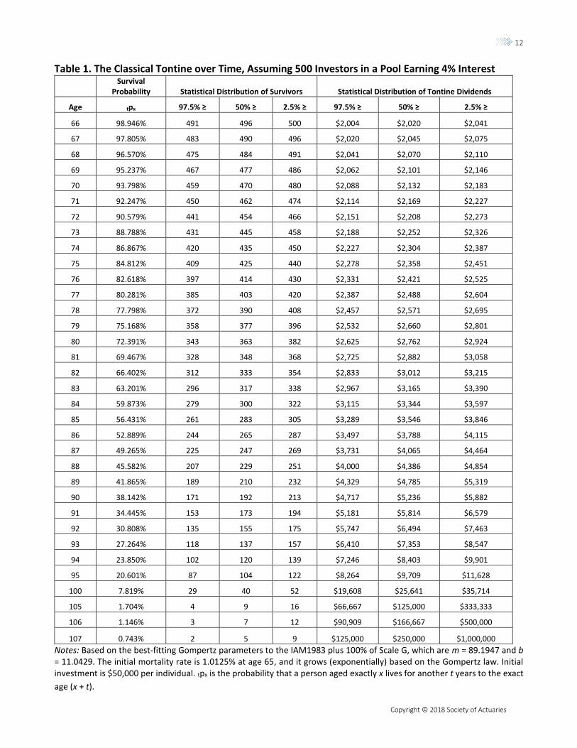
Table 1. The Classical Tontine over Time, Assuming 500 Investors in a Pool Earning 4% Interest

Survival Probability Statistical Distribution of Survivors Statistical Distribution of Tontine Dividends

Age tpx 97.5% ≥ 50% ≥ 2.5% ≥ 97.5% ≥ 50% ≥ 2.5% ≥

66 98.946% 491 496 500 $2,004 $2,020 $2,041

67 97.805% 483 490 496 $2,020 $2,045 $2,075

68 96.570% 475 484 491 $2,041 $2,070 $2,110

69 95.237% 467 477 486 $2,062 $2,101 $2,146

70 93.798% 459 470 480 $2,088 $2,132 $2,183

71 92.247% 450 462 474 $2,114 $2,169 $2,227

72 90.579% 441 454 466 $2,151 $2,208 $2,273

73 88.788% 431 445 458 $2,188 $2,252 $2,326

74 86.867% 420 435 450 $2,227 $2,304 $2,387

75 84.812% 409 425 440 $2,278 $2,358 $2,451

76 82.618% 397 414 430 $2,331 $2,421 $2,525

77 80.281% 385 403 420 $2,387 $2,488 $2,604

78 77.798% 372 390 408 $2,457 $2,571 $2,695

79 75.168% 358 377 396 $2,532 $2,660 $2,801

80 72.391% 343 363 382 $2,625 $2,762 $2,924

81 69.467% 328 348 368 $2,725 $2,882 $3,058

82 66.402% 312 333 354 $2,833 $3,012 $3,215

83 63.201% 296 317 338 $2,967 $3,165 $3,390

84 59.873% 279 300 322 $3,115 $3,344 $3,597

85 56.431% 261 283 305 $3,289 $3,546 $3,846

86 52.889% 244 265 287 $3,497 $3,788 $4,115

87 49.265% 225 247 269 $3,731 $4,065 $4,464

88 45.582% 207 229 251 $4,000 $4,386 $4,854

89 41.865% 189 210 232 $4,329 $4,785 $5,319

90 38.142% 171 192 213 $4,717 $5,236 $5,882

91 34.445% 153 173 194 $5,181 $5,814 $6,579

92 30.808% 135 155 175 $5,747 $6,494 $7,463

93 27.264% 118 137 157 $6,410 $7,353 $8,547

94 23.850% 102 120 139 $7,246 $8,403 $9,901

95 20.601% 87 104 122 $8,264 $9,709 $11,628

100 7.819% 29 40 52 $19,608 $25,641 $35,714

105 1.704% 4 9 16 $66,667 $125,000 $333,333

106 1.146% 3 7 12 $90,909 $166,667 $500,000

107 0.743% 2 5 9 $125,000 $250,000 $1,000,000

Notes: Based on the best-fitting Gompertz parameters to the IAM1983 plus 100% of Scale G, which are m = 89.1947 and b = 11.0429. The initial mortality rate is 1.0125% at age 65, and it grows (exponentially) based on the Gompertz law. Initial investment is $50,000 per individual. tpx is the probability that a person aged exactly x lives for another t years to the exact

age (x + t).

13


Here is how to interpret the numbers. Assume that a group of 500 investors, contributors or club

members are exactly 65 years old and invest $50,000 into a tontine pool for a total pool size of $25

million. The money is used to purchase a (very long dated) bond yielding 4% per annum, or $1,000,000

to the pool. Every year the survivors distribute the $1,000,000 among themselves. Table 1 displays the

median payouts over time, which increase from $2,000 (for those aged 65) to $25,641 for the lucky

handful who might survive to age of 100. In fact, if 29 or fewer investors survive to age 100 (an event

representing the 2.5% tail probability) but all the other people in the pool die earlier, their payout that

year would be at least $35,714. We will get much more precise on how exactly these probabilities are

computed, but the key takeaway here is as follows. In a classical tontine, the payments are initially

quite low. It would be the risk-free rate at best, and certainly much less than what a life annuity would

offer. The payments increase to the survivors and will soon exceed what the annuity would have

provided almost surely.

The last few survivors could receive 10 times their original ($50,000) investment—in one year alone.

Needless to say, this sort of picture lends itself to salacious plots for crime novels, even TV shows, and

hence tontines’ sordid reputation.

Getting to the point, we are not advocating for the resurrection of this form of investment tontine,

which leads to the increasing payments displayed in Table 1. Instead, we investigate a product that is

designed to naturally “levelize” or flatten the tontine payments over time by (so to speak) investing

the initial pool of funds in a portfolio of risk-free bonds whose coupons or maturity values decline

naturally over time. One offsets the other. All of this will be explained carefully in the next section.

Note that we will use the term Lorenzo tontine when discussing the historical structure displayed in

Table 1—in which payments increase (super-) exponentially—and use the term natural when focusing

on the RIT that is engineered to pay out level or flat cash flows in expectation. We are now ready—

after explaining the product we don’t want anyone to sell or buy—to examine the natural tontine.

14


3. More Recent History: Back to the Year 1986

Assume that someone retired (in Canada) at the age of 65 in early January 1986. Instead of using

$50,000 from their tax-sheltered retirement account (aka RRSP using Canadian terminology) to

purchase a life annuity—which at the time guaranteed $5,850 per year for life according to our

historical database6—they allocated or invested the funds in a natural tontine that attempted to flatten

or levelize payments. Here is the question: How would their tontine dividends or disbursements have

evolved during the next 30 years? How would that have compare with the fixed and guaranteed

alternative of $5,850 from a life annuity?

Once again, a natural tontine is distinct from a Lorenzo tontine. It is a very specific type of longevity

pooling arrangement in which a group of people (aka a syndicate) invest equal sums of money in a

portfolio of staggered zero-coupon bonds. The maturity values are preselected to exactly match the

estimated survival probabilities of the initial group or syndicate. Under the natural design the cash

payments flowing to the syndicate decline over time, which is in contrast to the classical (Lorenzo)

tontine in which the cash flows remain constant. The diminishing numerator is shared among an

equivalently diminishing denominator of survivors. The financial logic is really quite simple. A retiree—

as long as he or she is still alive—can expect a disbursement that remains (roughly) constant instead of

growing (super-) exponentially over time. The last survivor does not win an outsized longevity insurance

lottery, which among other (optical) benefits also reduces any moral hazard.

Here is how to think about the (rather simple) financial engineering. If the conditional survival

probability to the age of 90—corresponding with payments to be made in 25 years—is estimated to be

38%, then the syndicate will purchase just the right amount of bonds so that cash flows distributed

(i.e., the numerator) in year 25 will be approximately 38% of the cash flows distributed in the initial

year of the tontine. The size of syndicate shrinks and so does the pot of money.

6 The source for the data is CANNEX Financial Exchanges, and the $5,850 was the imputed annual average for males and

females across all insurance companies quoting annuities in January 1986. We will get more refined (i.e., monthly and gender specific) in the next section.

15


We say approximately 38% because even in the first year of the natural tontine’s life some mortality

or decrements are expected to be experienced. In fact, that is the (only) technical or mathematical

challenge we face when constructing the natural tontine. The only financial engineering question of

note is: How much money should the syndicate invest in each of the zero-coupon bonds—maturing

over the maximum lifetime of the pool—so that the numerator and denominator decline at the same

rate?

Now, although it is quite intuitive to build a tontine this way, the rationale for this design and a

discussion of its economic optimality properties were given in an earlier article7 aimed at a more

mathematical and actuarial audience. It’s actually an optimal contract (for those with logarithmic

utility) and not just an intuitive one.

For readers interested in a deeper understanding of why, we refer to that earlier work as well as the

various articles listed in the references section. Here we simply offer some numerical values for

payouts. All in all, the aggregate cash flow patterns, as well as the projected individual disbursements

over time, are displayed in Table 2.

7 See Milevsky and Salisbury (2015).

16


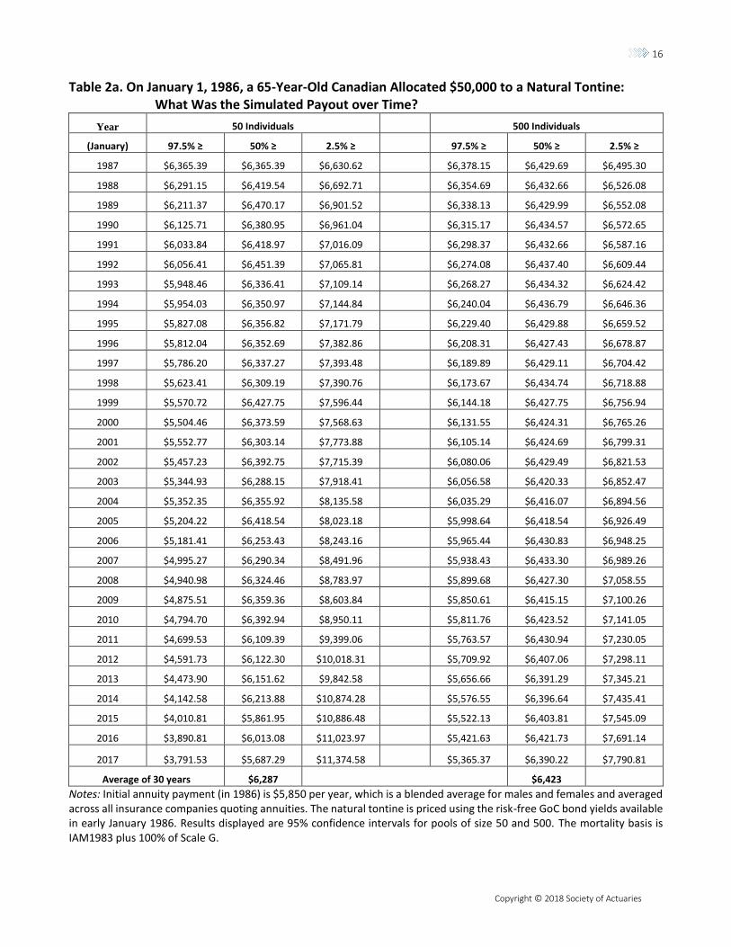
Table 2a. On January 1, 1986, a 65-Year-Old Canadian Allocated $50,000 to a Natural Tontine: What Was the Simulated Payout over Time?

Year 50 Individuals 500 Individuals

(January) 97.5% ≥ 50% ≥ 2.5% ≥ 97.5% ≥ 50% ≥ 2.5% ≥

1987 $6,365.39 $6,365.39 $6,630.62 $6,378.15 $6,429.69 $6,495.30

1988 $6,291.15 $6,419.54 $6,692.71 $6,354.69 $6,432.66 $6,526.08

1989 $6,211.37 $6,470.17 $6,901.52 $6,338.13 $6,429.99 $6,552.08

1990 $6,125.71 $6,380.95 $6,961.04 $6,315.17 $6,434.57 $6,572.65

1991 $6,033.84 $6,418.97 $7,016.09 $6,298.37 $6,432.66 $6,587.16

1992 $6,056.41 $6,451.39 $7,065.81 $6,274.08 $6,437.40 $6,609.44

1993 $5,948.46 $6,336.41 $7,109.14 $6,268.27 $6,434.32 $6,624.42

1994 $5,954.03 $6,350.97 $7,144.84 $6,240.04 $6,436.79 $6,646.36

1995 $5,827.08 $6,356.82 $7,171.79 $6,229.40 $6,429.88 $6,659.52

1996 $5,812.04 $6,352.69 $7,382.86 $6,208.31 $6,427.43 $6,678.87

1997 $5,786.20 $6,337.27 $7,393.48 $6,189.89 $6,429.11 $6,704.42

1998 $5,623.41 $6,309.19 $7,390.76 $6,173.67 $6,434.74 $6,718.88

1999 $5,570.72 $6,427.75 $7,596.44 $6,144.18 $6,427.75 $6,756.94

2000 $5,504.46 $6,373.59 $7,568.63 $6,131.55 $6,424.31 $6,765.26

2001 $5,552.77 $6,303.14 $7,773.88 $6,105.14 $6,424.69 $6,799.31

2002 $5,457.23 $6,392.75 $7,715.39 $6,080.06 $6,429.49 $6,821.53

2003 $5,344.93 $6,288.15 $7,918.41 $6,056.58 $6,420.33 $6,852.47

2004 $5,352.35 $6,355.92 $8,135.58 $6,035.29 $6,416.07 $6,894.56

2005 $5,204.22 $6,418.54 $8,023.18 $5,998.64 $6,418.54 $6,926.49

2006 $5,181.41 $6,253.43 $8,243.16 $5,965.44 $6,430.83 $6,948.25

2007 $4,995.27 $6,290.34 $8,491.96 $5,938.43 $6,433.30 $6,989.26

2008 $4,940.98 $6,324.46 $8,783.97 $5,899.68 $6,427.30 $7,058.55

2009 $4,875.51 $6,359.36 $8,603.84 $5,850.61 $6,415.15 $7,100.26

2010 $4,794.70 $6,392.94 $8,950.11 $5,811.76 $6,423.52 $7,141.05

2011 $4,699.53 $6,109.39 $9,399.06 $5,763.57 $6,430.94 $7,230.05

2012 $4,591.73 $6,122.30 $10,018.31 $5,709.92 $6,407.06 $7,298.11

2013 $4,473.90 $6,151.62 $9,842.58 $5,656.66 $6,391.29 $7,345.21

2014 $4,142.58 $6,213.88 $10,874.28 $5,576.55 $6,396.64 $7,435.41

2015 $4,010.81 $5,861.95 $10,886.48 $5,522.13 $6,403.81 $7,545.09

2016 $3,890.81 $6,013.08 $11,023.97 $5,421.63 $6,421.73 $7,691.14

2017 $3,791.53 $5,687.29 $11,374.58 $5,365.37 $6,390.22 $7,790.81

Average of 30 years $6,287 $6,423

Notes: Initial annuity payment (in 1986) is $5,850 per year, which is a blended average for males and females and averaged across all insurance companies quoting annuities. The natural tontine is priced using the risk-free GoC bond yields available in early January 1986. Results displayed are 95% confidence intervals for pools of size 50 and 500. The mortality basis is IAM1983 plus 100% of Scale G.

17


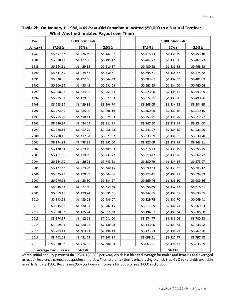
Table 2b. On January 1, 1986, a 65-Year-Old Canadian Allocated $50,000 to a Natural Tontine:

What Was the Simulated Payout over Time?

Year 1,000 Individuals 5,000 Individuals

(January) 97.5% ≥ 50% ≥ 2.5% ≥ 97.5% ≥ 50% ≥ 2.5% ≥

1987 $6,397.38 $6,436.19 $6,482.07 $6,416.73 $6,433.59 $6,453.16

1988 $6,380.47 $6,432.66 $6,499.12 $6,407.77 $6,433.98 $6,461.73

1989 $6,364.11 $6,429.99 $6,510.87 $6,400.83 $6,433.98 $6,468.83

1990 $6,347.89 $6,434.57 $6,530.61 $6,395.61 $6,434.57 $6,475.38

1991 $6,338.06 $6,432.66 $6,544.29 $6,389.07 $6,434.03 $6,481.03

1992 $6,320.85 $6,430.42 $6,551.08 $6,383.39 $6,434.60 $6,486.64

1993 $6,308.98 $6,434.32 $6,564.74 $6,378.00 $6,434.32 $6,493.09

1994 $6,295.01 $6,429.55 $6,577.53 $6,372.21 $6,433.90 $6,498.26

1995 $6,285.39 $6,429.88 $6,596.70 $6,366.95 $6,434.32 $6,504.65

1996 $6,272.46 $6,435.00 $6,606.19 $6,360.09 $6,433.48 $6,510.15

1997 $6,255.35 $6,429.11 $6,621.03 $6,353.91 $6,433.78 $6,517.27

1998 $6,240.69 $6,434.74 $6,641.25 $6,347.90 $6,433.14 $6,524.00

1999 $6,228.14 $6,427.75 $6,658.23 $6,341.57 $6,434.35 $6,531.59

2000 $6,210.16 $6,432.84 $6,672.07 $6,333.59 $6,434.55 $6,538.78

2001 $6,194.33 $6,433.55 $6,692.00 $6,327.09 $6,433.55 $6,545.51

2002 $6,180.84 $6,429.49 $6,709.03 $6,318.73 $6,433.19 $6,553.79

2003 $6,161.30 $6,429.99 $6,733.77 $6,310.42 $6,433.86 $6,562.22

2004 $6,144.70 $6,426.21 $6,745.92 $6,300.79 $6,434.34 $6,573.67

2005 $6,122.62 $6,429.26 $6,780.15 $6,290.63 $6,433.55 $6,583.12

2006 $6,095.78 $6,430.83 $6,804.86 $6,279.41 $6,433.11 $6,594.53

2007 $6,076.53 $6,433.30 $6,834.57 $6,269.44 $6,433.30 $6,605.96

2008 $6,046.33 $6,427.30 $6,859.50 $6,256.89 $6,432.53 $6,618.31

2009 $6,019.15 $6,429.24 $6,899.31 $6,242.65 $6,432.07 $6,633.35

2010 $5,993.38 $6,423.52 $6,938.07 $6,229.78 $6,432.76 $6,649.41

2011 $5,945.88 $6,430.94 $6,982.16 $6,211.89 $6,430.94 $6,669.64

2012 $5,908.92 $6,425.74 $7,019.20 $6,194.57 $6,433.24 $6,686.98

2013 $5,876.17 $6,412.11 $7,081.00 $6,174.77 $6,433.06 $6,709.33

2014 $5,819.01 $6,420.24 $7,130.68 $6,148.00 $6,429.73 $6,738.52

2015 $5,773.13 $6,403.81 $7,189.19 $6,125.83 $6,430.83 $6,767.80

2016 $5,702.05 $6,421.73 $7,268.55 $6,096.21 $6,427.97 $6,797.93

2017 $5,630.98 $6,426.32 $7,386.09 $6,063.21 $6,426.32 $6,835.69

Average over 30 years $6,428 $6,433

Notes: Initial annuity payment (in 1986) is $5,850 per year, which is a blended average for males and females and averaged across all insurance companies quoting annuities. The natural tontine is priced using the risk-free GoC bond yields available in early January 1986. Results are 95% confidence intervals for pools of size 1,000 and 5,000.

18


Table 2 shows results for a hypothetical group of 50, 500, 1,000 and 5,000 retirees who each invested

or contributed $50,000 to the tontine. Although the so-called premium of $50,000 would be relatively

modest for a middle-class retiree, the aggregate (time 0) investment fund would be $2.5 million, $25

million, $50 million and $250 million, respectively, which will surely and quickly attract the attention of

regulators.

Nevertheless, the tontine fund would be invested in a staggered portfolio of safe zero-coupon bonds.

Eyeballing the numbers in Table 2 (and the four averages on the bottom), one can see that regardless

of the size of the pool, each surviving retiree can anticipate receiving about $6,300 to $6,400 (plus or

minus a few dollars) per year during the period from January 1987 to January 2017. We could have

obviously projected further into the future—2018 and beyond, given the hypothetical nature of our

exercise—but we felt that 30 years of retirement was a natural ending point for the natural tontine.

Back to the $5,850 from the annuity. Here is our initial take-away from the 1986 run: The anticipated

natural tontine payment was more than $500 (or almost 10%) greater per year than the single premium

income annuity. The tontine doesn’t perform any longevity miracles, but its expected payments are

slightly higher—for this particular starting year—relative to the single-premium income annuity. With

hindsight and if all you cared about was the first year’s money, the RIT (sold by a nonprofit) would beat

the life annuity. Needless to say, that number is only an average and comes dangerously close to

claiming that a diversified portfolio of stocks can also beat a life annuity on average. We will get to the

risk in a moment, and in the next section will show that the 10% initial margin (of victory over the

annuity) doesn’t apply in general.

Nevertheless, the averages reported do assume that the underlying law of mortality (aka basis) evolved

according to the Individual Annuity Mortality (IAM) 1983 (unisex) table with full Scale G projections

from 1986 to 2017. We refer interested readers to the technical appendix in this paper, which explains

the process as well as how we parameterized the Gompertz law of mortality based on these numbers.

Under this law or basis, life expectancy at age 65 was 21.2 years with a standard deviation of 9.8 years.

This, by the way, would have been the table used in 1986 to price (or actually reserve for) many life

annuities sold by insurance companies. It’s why this particular table has been used.

19


Also, to be clear, the middle cell in each of the syndicate (N = 50, N = 500, N = 1000, N = 5000) columns

represents a median payment conditional on survival. There is a nontrivial probability that—in any

group of N people—realized mortality is lower (higher) and the analogous tontine disbursements are

(lower) higher even in the underlying actuarial basis was correct. This is so-called idiosyncratic risk.

In Table 2 we display the corresponding 2.5th and 97.5th percentiles in adjacent cells, offering a 95%

confidence interval using the assumed mortality basis for total disbursements. These numbers bracket

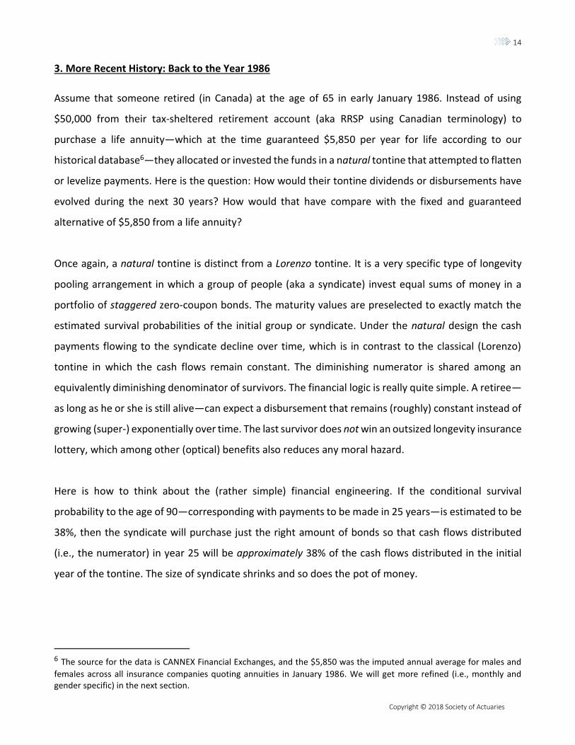
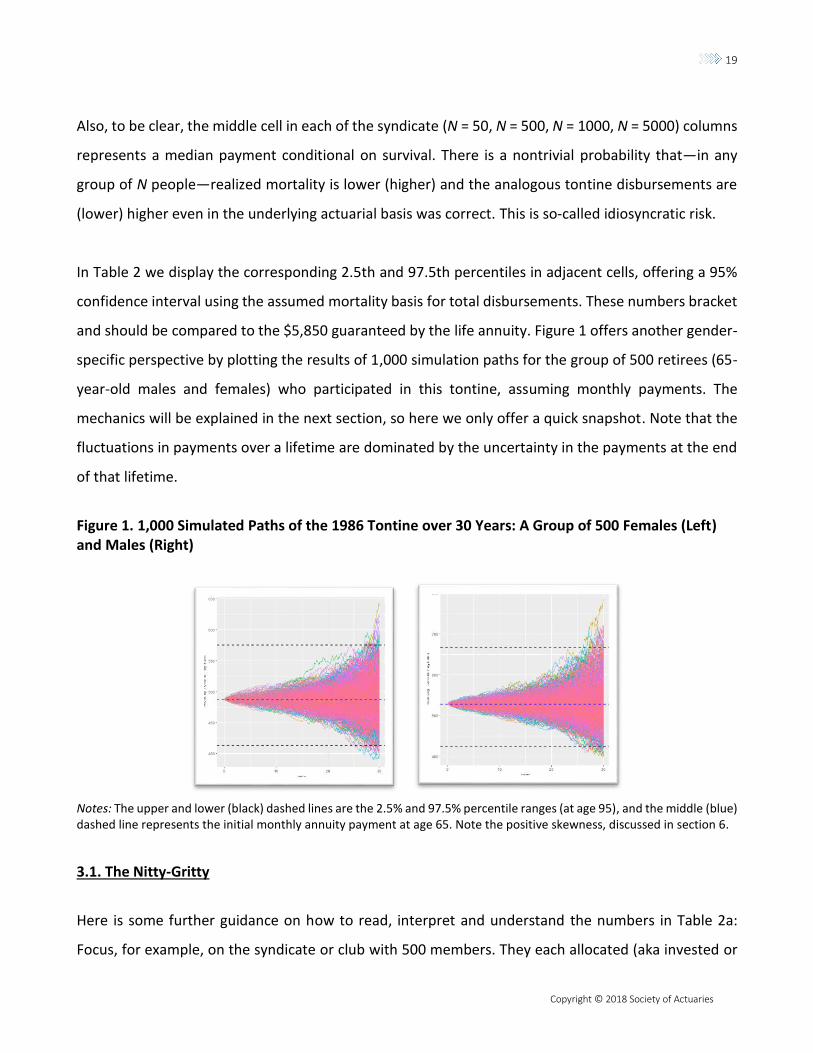
and should be compared to the $5,850 guaranteed by the life annuity. Figure 1 offers another gender-

specific perspective by plotting the results of 1,000 simulation paths for the group of 500 retirees (65-

year-old males and females) who participated in this tontine, assuming monthly payments. The

mechanics will be explained in the next section, so here we only offer a quick snapshot. Note that the

fluctuations in payments over a lifetime are dominated by the uncertainty in the payments at the end

of that lifetime.

Figure 1. 1,000 Simulated Paths of the 1986 Tontine over 30 Years: A Group of 500 Females (Left) and Males (Right)

Notes: The upper and lower (black) dashed lines are the 2.5% and 97.5% percentile ranges (at age 95), and the middle (blue) dashed line represents the initial monthly annuity payment at age 65. Note the positive skewness, discussed in section 6.

3.1. The Nitty-Gritty

Here is some further guidance on how to read, interpret and understand the numbers in Table 2a:

Focus, for example, on the syndicate or club with 500 members. They each allocated (aka invested or

20


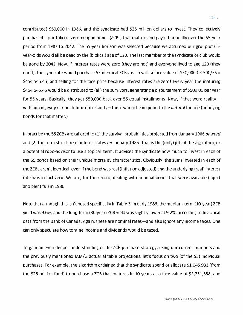
contributed) $50,000 in 1986, and the syndicate had $25 million dollars to invest. They collectively

purchased a portfolio of zero-coupon bonds (ZCBs) that mature and payout annually over the 55-year

period from 1987 to 2042. The 55-year horizon was selected because we assumed our group of 65-

year-olds would all be dead by the (biblical) age of 120. The last member of the syndicate or club would

be gone by 2042. Now, if interest rates were zero (they are not) and everyone lived to age 120 (they

don’t), the syndicate would purchase 55 identical ZCBs, each with a face value of $50,0000 × 500/55 =

$454,545.45, and selling for the face price because interest rates are zero! Every year the maturing

$454,545.45 would be distributed to (all) the survivors, generating a disbursement of $909.09 per year

for 55 years. Basically, they get $50,000 back over 55 equal installments. Now, if that were reality—

with no longevity risk or lifetime uncertainty—there would be no point to the natural tontine (or buying

bonds for that matter.)

In practice the 55 ZCBs are tailored to (1) the survival probabilities projected from January 1986 onward

and (2) the term structure of interest rates on January 1986. That is the (only) job of the algorithm, or

a potential robo-advisor to use a topical term. It advises the syndicate how much to invest in each of

the 55 bonds based on their unique mortality characteristics. Obviously, the sums invested in each of

the ZCBs aren’t identical, even if the bond was real (inflation adjusted) and the underlying (real) interest

rate was in fact zero. We are, for the record, dealing with nominal bonds that were available (liquid

and plentiful) in 1986.

Note that although this isn’t noted specifically in Table 2, in early 1986, the medium-term (10-year) ZCB

yield was 9.6%, and the long-term (30-year) ZCB yield was slightly lower at 9.2%, according to historical

data from the Bank of Canada. Again, these are nominal rates—and also ignore any income taxes. One

can only speculate how tontine income and dividends would be taxed.

To gain an even deeper understanding of the ZCB purchase strategy, using our current numbers and

the previously mentioned IAM/G actuarial table projections, let’s focus on two (of the 55) individual

purchases. For example, the algorithm ordained that the syndicate spend or allocate $1,045,932 (from

the $25 million fund) to purchase a ZCB that matures in 10 years at a face value of $2,731,658, and

21


spend or allocate $41,864 to purchase a ZCB that matures in 30 years at a face value of $661,438. In 10

years (i.e., 1996) the maturing $2,731,658 would be disbursed among the group of survivors.

Much later, in 30 years (i.e., 2016), the $661,438 would be disbursed among the (much smaller) group

of survivors. Continuing with the so-called 500 club, let’s focus on year 25, which represents January

2011. The anticipated (median) disbursement to each member according to Table 2a is $6,431. This

again assumes that mortality evolves according to plan (IAM1983, projected with Scale G) and 38% of

the group survives. Just to be clear, that means the 190 retirees from the 500 who are 90-year-olds.

(Who exactly? We have no idea.)

But what if a tail (or at least unexpected) event occurs? What if the number of survivors is (much)

higher in 2011? What if the number of survivors is so great that it could only happen (by random

chance) with a 2.5% probability using the initial actuarial basis? In that case the tontine payout would

be $5,764 (or less) in 2011 to that (larger) group of survivors.

This is one of our key messages. What are the benefits of taking on this (2.5% tail) risk? Well, on the

other side of the coin if the syndicate experienced above average mortality– to the same tune of 2.5%—

and a particular retiree was lucky enough to be one of the survivors, the disbursement would have

been $7,230. Notice the positive skewness in payouts—the fingerprint of the natural or levelized

tontine—which is something we will return to in section 6. It is the upside to the natural tontine’s

downside. This is the expected return to compensate for the risk—the longevity risk tradeoff. Overall,

the 95% confidence interval for disbursements in 2011 (at age 90) is from $5,764 to $7,230 (a spread

of $1,432).

Moving on, Table 2b also displays these intervals or ranges for different (initial) tontine group sizes and

the 30 years of disbursements from 1987 to 2017. Remember that although this is an historical

(backward-looking) analysis, it is hypothetical in the sense that we have not identified (or selected) a

specific group of Canadians who in 1986 purchased the tontine. The best we can do is report a 95%

confidence interval using the assumed mortality basis.

22


In theory, yes, we could go back to a named and identified group of retirees—perhaps members of a

particular pension plan or group of known university professors—and assume every single one of them

allocated $50,000 to the natural tontine. We would then track the payments of (say, John Smith,

member 310) over time. In that case there would be no uncertainty to report or randomness to

capture. Every payment would have been known (and deterministic) conditional on the life paths of

the other 499 members until 2016. To be clear, what we have performed is a probabilistic

representation of the outcome for 1986 only. How this might have played out for another group of

tontine investors of 1987, or 1997, will be revealed in the next section.

One of the many caveats worth mentioning at this point are as follows: First, as far as the zero-coupon

(or any) bonds are concerned, in 1986 we were unable to find (or price) Canadian bonds that matured

beyond 25 years. To complete the missing years from year 26 to 55 we assumed such bonds existed

(they don’t) and assumed their yield was the same as the (final) 25-year bond (they probably wouldn’t

be). This is a flat yield curve assumption and is one of the concerns that must be dealt with carefully

and transparently in practice. Operationally there is some reinvestment or rollover strategy risk that

must be managed over time that creates some additional risk for the natural tontines. Also, another

important point is the actual curve itself. Perhaps corporate bonds could be used, which would increase

the yield relative to the annuity, but that obviously introduces default risk. We are concerned that using

risky bonds—which insurance companies obviously include in their general account—would defeat the

purpose or intent of the transparent and risk-free nature of the natural tontine. Indeed, as retirees age

they need (safe) bonds in their asset mix according to any life-cycle model of portfolio theory. Why not

wrap a tontine scheme around the (safe) bonds you already hold?

Nevertheless, to even out the playing field and make the comparison more meaningful, we have also

included some results—using the exact same pricing methodology—but assuming the tontine funds

are invested in (manufactured zero coupon) corporate bonds instead of government bonds. Of course,

whether we purchase 55 government bonds (more liquid) or 55 corporate bonds (less liquid) we have

also ignored the nontrivial commissions and legal fees required to manage the tontine (trust). In other

words, the 10% premium over the annuity payout (in 1986) might be hiding some yet-to-be-charged

fees. In that sense, the guaranteed life annuity has its advantages.

23


Another (ignored) risk in Table 2 is the systematic component of mortality. While our 95% confidence

bands accounted for the nonsystematic variation in mortality, one always confronts the risk that the

underlying force of mortality (is stochastic and) doesn’t evolve according to the assumed law or basis,

in which case the confidence bands are too small. We will address these ”bigger” risks in section 5.

Again, if these risks are unacceptable, there is always the life annuity. Or, here is a thought, why not

diversify and hold both?

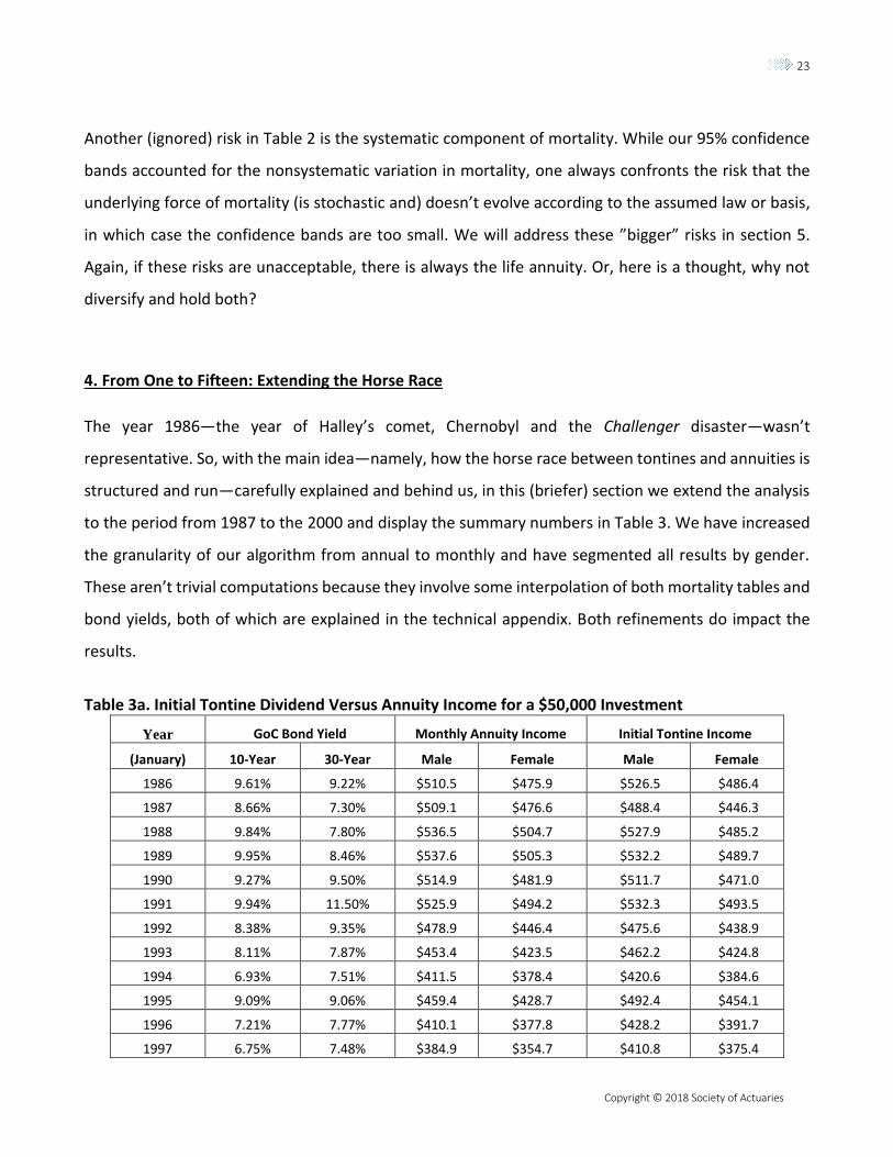
4. From One to Fifteen: Extending the Horse Race

The year 1986—the year of Halley’s comet, Chernobyl and the Challenger disaster—wasn’t

representative. So, with the main idea—namely, how the horse race between tontines and annuities is

structured and run—carefully explained and behind us, in this (briefer) section we extend the analysis

to the period from 1987 to the 2000 and display the summary numbers in Table 3. We have increased

the granularity of our algorithm from annual to monthly and have segmented all results by gender.

These aren’t trivial computations because they involve some interpolation of both mortality tables and

bond yields, both of which are explained in the technical appendix. Both refinements do impact the

results.

Table 3a. Initial Tontine Dividend Versus Annuity Income for a $50,000 Investment

Year GoC Bond Yield Monthly Annuity Income Initial Tontine Income

(January) 10-Year 30-Year Male Female Male Female

1986 9.61% 9.22% $510.5 $475.9 $526.5 $486.4

1987 8.66% 7.30% $509.1 $476.6 $488.4 $446.3

1988 9.84% 7.80% $536.5 $504.7 $527.9 $485.2

1989 9.95% 8.46% $537.6 $505.3 $532.2 $489.7

1990 9.27% 9.50% $514.9 $481.9 $511.7 $471.0

1991 9.94% 11.50% $525.9 $494.2 $532.3 $493.5

1992 8.38% 9.35% $478.9 $446.4 $475.6 $438.9

1993 8.11% 7.87% $453.4 $423.5 $462.2 $424.8

1994 6.93% 7.51% $411.5 $378.4 $420.6 $384.6

1995 9.09% 9.06% $459.4 $428.7 $492.4 $454.1

1996 7.21% 7.77% $410.1 $377.8 $428.2 $391.7

1997 6.75% 7.48% $384.9 $354.7 $410.8 $375.4

24


1998 5.52% 5.89% $364.9 $333.9 $371.4 $334.7

1999 4.90% 5.15% $347.0 $315.2 $348.1 $311.7

2000 6.36% 5.99% $373.1 $341.1 $391.0 $353.4

Notes: The (hypothetical) natural tontine is priced using the entire GoC (zero coupon) bond curve observed for January of the year in question. The mortality basis is IAM1983 plus 100% of Scale G, but the tontine payment doesn’t include any loading, fees or commissions. See the concluding section for more on this. The annuity payouts are based on real (average company) quotes and adjusted to be life-only and obviously include insurance loadings and embedded commissions.

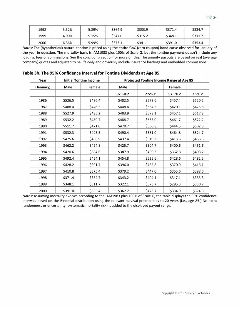
Table 3b. The 95% Confidence Interval for Tontine Dividends at Age 85

Year Initial Tontine Income Projected Tontine Income Range at Age 85

(January) Male Female Male Female

97.5% ≥ 2.5% ≥ 97.5% ≥ 2.5% ≥

1986 $526.5 $486.4 $482.5 $578.6 $457.4 $520.2

1987 $488.4 $446.3 $448.4 $534.5 $420.1 $475.8

1988 $527.9 $485.2 $483.9 $578.1 $457.1 $517.3

1989 $532.2 $489.7 $488.7 $583.0 $461.7 $522.2

1990 $511.7 $471.0 $470.7 $560.8 $444.5 $502.3

1991 $532.3 $493.5 $490.4 $581.0 $464.8 $524.7

1992 $475.6 $438.9 $437.4 $519.3 $413.6 $466.6

1993 $462.2 $424.8 $425.7 $504.7 $400.6 $451.6

1994 $420.6 $384.6 $387.9 $459.3 $362.8 $408.7

1995 $492.4 $454.1 $454.8 $535.6 $428.6 $482.5

1996 $428.2 $391.7 $396.0 $465.8 $370.9 $416.1

1997 $410.8 $375.4 $379.2 $447.0 $355.6 $398.6

1998 $371.4 $334.7 $343.2 $404.1 $317.1 $355.3

1999 $348.1 $311.7 $322.1 $378.7 $295.3 $330.7

2000 $391.0 $353.4 $362.2 $423.7 $334.9 $374.8

Notes: Assuming mortality evolves according to the IAM1983 plus 100% of Scale G, the table displays the 95% confidence intervals based on the Binomial distribution using the relevant survival probabilities to 20 years (i.e., age 85.) No extra randomness or uncertainty (systematic mortality risk) is added to the displayed payout range.

25


Table 3c. The Corporate (Versus Government) Bond-Backed Tontine

Year Corporate Bond Yield Annuity Income Initial Tontine Income

(January) 10-Year 30-Year Male Female Male Female

1986 11.40% 11.01% $510.5 $475.9 $592.0 $552.5

1987 11.10% 9.74% $509.1 $476.6 $578.5 $537.6

1988 12.61% 10.56% $536.5 $504.7 $633.1 $592.3

1989 12.45% 10.96% $537.6 $505.3 $628.4 $587.3

1990 10.88% 11.11% $514.9 $481.9 $572.4 $532.0

1991 9.76% 11.32% $525.9 $494.2 $525.7 $486.9

1992 9.06% 10.02% $478.9 $446.4 $499.0 $462.4

1993 10.08% 9.84% $453.4 $423.5 $531.5 $494.6

1994 7.16% 7.74% $411.5 $378.4 $428.3 $392.3

1995 10.26% 10.23% $459.4 $428.7 $535.2 $497.3

1996 7.51% 8.06% $410.1 $377.8 $438.1 $401.7

1997 6.91% 7.64% $384.9 $354.7 $415.9 $380.6

1998 5.93% 6.30% $364.9 $333.9 $384.9 $348.2

1999 5.82% 6.07% $347.0 $315.2 $378.2 $341.6

2000 7.68% 7.31% $373.1 $341.1 $436.9 $399.5

Table 3d. Initial Tontine Income and Projected Tontine Income Range at Age 85

Year Initial Tontine Income Projected Tontine Income Range at Age 85

(January) Male Female Male Female

97.5% ≥ 2.5% ≥ 97.5% ≥ 2.5% ≥

1986 $592.0 $552.5 $542.6 $650.6 $519.5 $590.8

1987 $578.5 $537.6 $531.2 $633.2 $506.0 $573.2

1988 $633.1 $592.3 $580.3 $693.3 $558.0 $631.6

1989 $628.4 $587.3 $577.0 $688.4 $553.8 $626.4

1990 $572.4 $532.0 $526.5 $627.2 $502.1 $567.4

1991 $525.7 $486.9 $484.3 $573.7 $458.5 $517.6

1992 $499.0 $462.4 $458.8 $544.7 $435.7 $491.6

1993 $531.5 $494.6 $489.5 $580.4 $466.4 $525.8

1994 $428.3 $392.3 $395.0 $467.8 $370.1 $416.9

1995 $535.2 $497.3 $494.4 $582.2 $469.4 $528.4

1996 $438.1 $401.7 $405.2 $476.6 $380.3 $426.6

1997 $415.9 $380.6 $383.9 $452.6 $360.4 $404.1

1998 $384.9 $348.2 $355.7 $418.8 $329.9 $369.6

1999 $378.2 $341.6 $349.9 $411.5 $323.6 $362.4

2000 $436.9 $399.5 $404.7 $473.5 $378.5 $423.6

26


Although the numbers follow the same structure and logic as Table 2, some important differences are

seen, and here are some of the main highlights. As we hinted in the prior section, the 10% magnitude

of the relative benefit of the tontine in 1986 wasn’t representative of subsequent years. For example,

to start, in January 1987, after a drop of 100 to 200 basis points in GoC bond yields, the initial tontine

payout was actually 4% less favorable for males and 6% less favorable for females, relative to the

relevant annuity payout.

In fact, there was one purchase year (female purchase in 1987) where by age 85 there was actually less

than a 2.5% chance the tontine would exceed the annuity. In the other direction, there was a year

(female purchase in 1997) where by age 85 there was less than a 2.5% chance that the annuity would

exceed the tontine. Typically the discrepancies were far less extreme, but this emphasizes that a single

year should not be the basis for comparisons.

It’s worth emphasizing at this critical juncture that part of the reason we obtained these results is that

GoC bond yields—which we use to engineer the natural tontine—are only weakly correlated with

annuity payouts. This is quite obvious to insurance practitioners, and the scientific evidence to back

this up was published in a recent academic article8 written by one of the co-authors of this paper.

Indeed, the takeaway in all of this should be clear. As we progress from the 1986 to the 2000 period,

the benefit of the natural tontine—engineered using GoC bonds—relative to the life annuity sold by

insurance companies (backed by higher yielding bonds, obviously) continued to deteriorate. However,

the two competitors are neck-and-neck over the entire 15 years.

In contrast to the results using government bonds (Table 3a, 3b), when corporate bonds are utilized as

the underlying investment asset, the higher initial yield enables the group or syndicate to acquire more

(future) income at a lower price, and the initial tontine payments are always higher than what a

comparable life annuity would have provided. Again, the proviso here is the these (corporate) RITs—

versus the government backed versions—now incur credit default risk and introduce a new element of

uncertainty into future payouts.

8 See Charupat, Kamstra and Milevsky (2016).

27


5. Models Can Be Fickle and Frail: What if Longevity Improves?

We must address some technical matters before wrapping up the statistical analysis, and that has to

do with the statistical range of tontine payouts we reported in the prior sections. Those numbers

assumed that (1) the tontine was issued or sold by a nonprofit entity with no loading or fees, something

even Vanguard can’t do, and more importantly we assumed that (2) mortality evolved as planned

according to the initial table in use at the time the time of issue. In some sense, we have ignored

aggregate longevity risk (and its cost) in the sense of systematic demographic uncertainty.

So in this (shorter) section we correct that omission. In particular, we report on the results of a

sensitivity analysis using an approach in which the initial mortality basis is perturbed or shocked by

(essentially) reducing participants mortality rates so that—and we say this with all caution—males

behave like females. This then implies that less people are dying and tontine dividends to the group are

correspondingly reduced.

The range of payouts will change to the detriment of the investors. Figure 2 displays what this would

imply in terms of payouts. It plots results assuming different values of a transformation or shifting

parameter (denoted by theta). It is equal to one when mortality evolves as expected, it is greater than

one when mortality is higher than planned and thus increases payouts to tontine survivors, and vice

versa when θ is less than 1. Without getting caught up in the actuarial minutia, think of this as shifting

the modal (not model) value of the future lifetime random variable. Either way, misestimating mortality

is yet another source of risk or uncertainty (adding to the second statistical moment) that a participant

in a natural tontine would be exposed to within the scheme.

28


Figure 2. Sensitivity Results: “Best and Worst-Case Scenario” for Females (Right) and Males (Left)

Note: The figure displays confidence intervals (as in Tables 2 and 3) but when the realized mortality differs from (is tilted away from) assumed. See the technical appendix for more details.

This sums up the historical statistical analysis of (hypothetical) RIT payments. Although the focus of this

paper is numerical and applied, the next section makes the argument that there are some additional

benefits to the tontine that can be appreciated only by examining and appealing to higher (third)

moments.

6. Skewness and Inflation

Going back to theoretical principles, in a frictionless economy in which (1) survival probabilities are

deterministic and (2) all longevity-contingent claims are priced off the same risk-free curve, there is at

most a small incremental value or utility from using tontines versus life annuities to hedge retirement

longevity risk. In fact, the empirical analysis we just displayed confirms how close they really are.

Moreover, as we emphasized in section 2, within a small pool the tontine generates an additional

source of idiosyncratic risk, namely, if an unexpectedly large number of people survive to old age and

payments are correspondingly reduced. From a fundamental economic point of view, as the size of the

pool goes to infinity, the payout from the natural tontine converges to the annuity, and then one of

the two is a redundant economic asset. They are both special cases of what Yaari in his landmark 1965

work called actuarial notes; see also the work by Davidoff, Brown and Diamond (2005), which proved

29


the generality of the Yaari result. The tontine is just another way to rearrange cash flows over time. It

offers nothing new or novel (at least to an academic economist).

One reason this might not be the case, and why an investor might find the tontine appealing, has been

alluded to earlier, namely, that tontine returns will inevitably be skewed. This skew provides a

dimension to tontine returns that is not present in the returns to the underlying fixed-income

investments. Table 4 provides a (hypothetical) example of what we mean by the natural tontine’s

statistical skew and how it would look in practice.

Table 4. The Natural Tontine and Its Skew

Age Expected Cash to Pool 95.0% ≥ 5.0% ≥ Upside Downside Skew

70 470.6 $3,491,184 $7,303.7 $7,573.1 $155.1 $114.2 35.79%

75 425.9 $3,159,669 $7,213.9 $7,669.1 $251.1 $204.1 23.05%

80 361.3 $2,680,407 $7,109.8 $7,791.9 $373.9 $308.1 21.35%

85 275.5 $2,043,688 $6,975.0 $7,952.1 $534.1 $442.9 20.60%

90 176.2 $1,306,827 $6,771.1 $8,271.1 $853.1 $646.8 31.89%

95 84.3 $625,233 $6,379.9 $8,806.1 $1,388.1 $1,038.0 33.73%

100 25.0 $185,422 $5,618.8 $10,907.2 $3,489.2 $1,799.1 93.94%

105 3.4 $24,994 $3,570.5 $24,993.8 $17,575.9 $3,847.4 356.82%

Note: Assumes a group of 500 people at the age of 65 who invest $100,000 each for a total pool size of $50,000,000. The assumed interest rate is a fixed 3.5% per annum, and the mortality basis is Gompertz with a modal value of 88.721 and dispersion parameter of 10. Under this mortality basis, the age 65 conditional survival probability to age 100 is exactly 5%, and the age 65 annuity factor is $13.4808. The (unloaded) fair annuity dividend agrees with the initial (time 0) tontine dividend and equals $7,418. Upside and downside are measured relative to this value.

In Table 4, we model a group of 500 investors, all at age 65, who each invest $100,000 into a natural

tontine for a total investment of $50 million. The funds are invested in zero-coupon bonds, exactly as

we described above, except that we assumed the term structure of interest rates is flat at 3.5%. The

cash that is distributed to the pool declines over time (naturally), and although the dividend per

survivor (and the initial dividend) is expected to be $7,418, it will obviously vary over time. We display

the upper end of the range (payments will exceed this value with 5% probability) and the lower end

(payments will exceed this value with 95% probability).

Now focus on the age of 95, which is 30 years after inception. The (deterministic, known, fixed) cash

flow to the pool is $625,233, but the tontine’s 90% confidence interval is between $6,380 and $8,806.

30


More importantly, the upside relative to the initial dividend is $8,806 − $7,418 = $1,388, but the

downside is only $7,418 − 6,380 = $1,038. The upside is approximately 34% greater than the downside,

and that is precisely what we mean by skewness. From a probabilistic perspective, the skewness can

be traced to fact we are dividing a fixed known amount by an (approximately) normally distributed

random variable. The inverse of a symmetric normal distribution isn’t normally distributed and

definitely isn’t symmetric. Some of the skewness (in tontine payments) will, however, dissipate as the

pool grows large.

We have an additional factor to consider, which may add to the investment appeal of tontines, and this

is our main point here. In a nonperfect and nonfrictionless economy in which survival probabilities

themselves are stochastic and state-contingent, the tontine’s random payout might offer an additional

hedging element absent from a life annuity’s deterministic income profile. In fact, counterintuitively,

small tontine pools could be preferred, and the associated risks might be welcomed. For example, if

states with lower (higher) longevity are associated with states of higher (lower) inflation, the tontine

(annuity) might actually be favored.

Here is the economic intuition underlying our finding for why a natural tontine might in fact, at times,

be preferred to a (level) life annuity despite expected incomes or cash flows being almost identical and

initial costs and entry prices being the same. (Or, more realistically, why individuals might optimally

choose to hold both products in their investment portfolio.) To understand this, consider the following

thought experiment: Imagine a rapidly growing economy such as China or India in which inflation is

expected or forecasted to be 5% per year (for example) and the mortality rate for an 85-year-old is

expected to be 5% (again, for example). In the event this emerging economy grows by more than

anticipated (aka overheats), it is quite plausible that the realized inflation rate will be greater than 5%

and the realized mortality rate for an 85-year-old will also be greater than 5%. Although the former

claim might seem obvious to a monetary economist, the latter requires some demographic

justification. In fact, an article by Bourne et. al. (2014) showed (or at least claimed) that mortality

increases a few years after a recession. This would be unexpected mortality in the traditional sense,

and the years after a recession are when inflation would be more likely to increase. Perhaps an

31


overheating economy damages the environment, increases industrial pollution or is associated with

more traffic fatalities.

The exact mechanism by which this is transmitted from economics to biology is not our concern, and

we certainly aren’t claiming causality. Rather, all we require is that states of nature in which inflation

is higher than expected are associated with states of nature in which death rates are higher than

expected. The state of the economy is a latent variable.

To understand this, it helps to think in terms of a numerator, which is the cash flows to the syndicate,

and a denominator, which is the number of survivors on any given date. Back to our story and main

premise: In the event of unexpectedly higher aggregate inflation, the number of survivors in the

denominator will be lower. So, yes, the chance that any given tontine participant has survived to age

85 is also lower, and they might not worry as much about that state of nature.

And yet, conditional on survival—which is required for calculating personal utility—the expected

number of other survivors is also lower. In other words, one’s colleagues in the denominator are

expected to be smaller, thus increasing the payments to the few survivors. This will happen precisely

in the states of nature in which the numerator is (subjectively) worth less because of the shock to

inflation. The end result in all of this is that those states of nature (i.e., excess inflationary) in which the

numerator’s subjective utility is reduced will be offset by those states of nature in which the

denominator is reduced—once again acting as a leveler of payments.

Of course, the correlation between shocks to mortality and shocks to inflation might indeed be

negative, in which case the effect is exactly the opposite and the natural tontine is worse compared to

the flat life annuity. In that case, excess background risk (aka inflation) is associated with lower

mortality rates, and there are now many more survivors competing for the scarce and less valuable

resource in the numerator. Yes, it could go the other way, but the empirical evidence seems to point

in the direction we need to make the tontine’s skewness—which is really what underlies it all—

something that is valued.

32


To our main point: If the upside (aka I’m alive and others are not) is experienced or earned in state of

nature in which the purchasing power of the payment is eroded, it will be valued more than the annuity

even if the expected cash flow (in our case $7,418) is exactly what the annuity would have guaranteed.

That, in a nut shell, is why a rational risk-averse consumer might actually accept this particular risk. In

the language of Arrow and Debreu, the states of nature in which the retirees are alive—and most of

his or her pool members are not—will be the states of nature in which they most value the

(unexpectedly) higher tontine payment.

Let us take this even further and imagine a world in which annuity product innovation has addressed

some of the above issues, by offering inflation-adjusted annuities. To be clear, a real inflation-adjusted

annuity sold by an insurance company would guarantee a constant real income stream—by investing

the assets in real return bonds—and the annuitant would be invariant to realized aggregate inflation.

However, we claim that even if annuities were to be redesigned to hedge aggregate (population)

inflation, investors would still be exposed to the discrepancy between aggregate inflation and the true

cost of their own (personal) desired consumption basket.

Bottom line: As a result of the tontine’s skewed returns, we find- that the tontine provides an additional

edge in hedging (personal, retirement) risk that is difficult to insure otherwise.

Perhaps one can think of this as the difference between a personal (idiosyncratic) inflation rate—which

is not “hedgeable”—distinct from the aggregate (population) index. Either way, the key is that there

would be a loss in utility (of consumption) from the real annuity income. If personal inflation was higher

than the aggregate inflation, the income payment would not provide the same level of utility compared

to the case in which personal inflation falls under the aggregate. Mathematically the annuity income

would be adjusted by this background risk, which one can think of as a multiple or factor whose

expected value is one.

Of course, what is good for the goose is good for the gander, and the exact same adjustment would be

made to the levelized tontine income, since the pool’s assets would be invested in the same real return

bonds exposed to the same background risk or inflation slippage. However, this is exactly where the

33


tontine’s group survivorship mechanism would (quite subtly) partially fix the problem, because the

skew means that higher mortality impacts returns more than lower mortality.

In other words, even if the income in the numerator is provided in real inflation-adjusted terms, if the

consumer price index used does not account for personal inflation, then there is some basis risk and

hedging benefit to the tontine.

7. Summary, Conclusion and Institutional Loose Ends

During the last two or three decades—with the increase in longevity, the global transition from DB

pension plans to DC investment schemes and the concern with what happens at the point of

retirement—there has been a revival of interest in the area of participating annuities in which mortality

risk is shared transparently and fully within a closed (or open) pool. In some sense, an RIT is yet another

type of participating annuity. We count at least 10 different proposals or schemes suggested by pension

specialists and scholars, most of which are referenced and citied in the bibliography. Note that many

involve using assets other than fixed-income bonds as the underlying investment vehicle, and we also

feel it would be a natural next step.

The current research work and paper ties into this strand of literature. In the spirit of the tontine’s

history we ask: How would the payout from fixed-income tontines compare with guaranteed life

annuities? Our answer isn’t quite clear-cut. In particular, it depends on whether one uses government

bonds or corporate bonds as the underlying asset backing the pool. Using (Canadian) government

bonds as the pricing basis, during the period 1986–2000, approximately 60% of the initial tontine

payments exceeded the initial life annuity. In 40% of the cases, the average life annuity issued by a

(Canadian) insurance company would have yielded or offered more. In contrast to the neck-and-neck

result, when using the (imputed) corporate bond curve, we find that 100% of initial tontine payments

would have exceeded the life annuity payouts at that time.

There are, however, various institutional issues that are not included in the above-mentioned odds,

and we can’t really address until such a product comes into existence. Here are just some of the issues

34


a tontine scheme might face in addition to the transaction costs and administrative fees we alluded to

earlier, or the considerable regulatory and legal costs that would be incurred during the first few years

of such a venture.

Dividends: Compensation to shareholders of the tontine corporation would be necessary if the tontine

were structured as a for-profit corporation. But markets and analysts (and even regulators) now tend

to prefer fee-based earnings as opposed to insurance or commission-based earnings. Note that price-

to-earning ratios typically are higher for asset managers in comparison to insurers. The fee to

administer a tontine would most likely be a percentage of assets under management, as is typical for

asset managers, so dividends to shareholders of the tontine corporation might well end up positioned

below those for shareholders of insurers. To put it bluntly, shareholders of a tontine corporation might

require a higher cost of capital, versus the shareholders of an insurance company selling life annuities.

Reserving costs: These would still be present but would be (much) lower for tontines versus annuities,

since reserving against basis risk or systematic longevity risk would no longer be required. There would

still be operational risk to consider as well as credit risk associated with assets, particularly if corporate

bonds, with higher returns, are allowed to substitute for government bonds.

As a result of these (and other) caveats, our take-away is that one must be very careful not to label any

RIT design as cheaper or more cost-effective compared to a single-premium life annuity sold by

insurance companies. Rather, the RIT is an alternative asset or product along the longevity risk-return

spectrum. Perhaps this is no different than the classic economic choice between risk-free cash (on the

one extreme) and risky stock (on the other.) Financial analysts are aware that stocks dominate cash in

expectation—and financial (academic) economists agree they offer greater utility for most levels of risk

aversion—but stocks shouldn’t be positioned as better than cash, or safer in the long run.

To be clear, the tontine versus annuity choice should not be positioned as an Uber versus taxi

comparison, as some have advocated. It’s a risk and return tradeoff, not an efficiency one. In fact, to

push the analogy even further, perhaps the comparison (or closest product type) is a so-called collared

equity fund (e.g., buy/write with equity options) versus straight and linear equity exposure. Needless

35


to say, equity options are expensive, and the volatility is unpredictable. One can’t expect money to

grow as fast or retirement wealth to be higher when invested in a protected mutual fund, but the fund’s

ongoing volatility will certainly be lower.

While on the topic of stocks or equity, although we have refrained from analyzing anything other than

government and corporate bonds as the underlying backbone of the RIT, in theory the tontine assets

could be invested in stocks, real estate, commodities or even Bitcoin and Etherium for that matter.

However, if the objective is conservative and predictable retirement income and pension

replacements, it’s unclear that the latter few would make sense.

To conclude with some insights from behavioral economics, we think it’s important—for both

regulatory and legal reasons—not to position or frame any RIT as yet another type of insurance product

that could be offered by an insurance company. Rather, we would position the 21st-century tontine as

a contractual arrangement between consenting adults in which a group of people buy financial assets

and agree to share the dividends and income in an unconventional way. Indeed, that could apply to

any asset class.

36


Selected Bibliography

Bodie, Z. 1990. Pensions as Retirement Income Insurance. Journal of Economic Literature 28, no. 1:28–49. Boyle, P., M. Hardy, A. MacKay and D. Saunders. 2015. Variable Payout Annuities. Schaumburg, IL: Society of Actuaries. Bourne, P.A., Charlene Sharpe-Pryce, Cynthia Francis, Ikhalfani Solan, Angela Hudson-Davis5, Jannine Campbell-Smith and Olive Watson-Coleman 2014, Mortality and Inflation: A 21-Year Analysis of Data on Jamaica, J Gen Pract 2:151. doi:10.4172/2329-9126.1000151 Caron, B., and C. Devine. 2017. Lifetime Income Solutions for DC Plans: Survival Sharing. Plan Consultant, Spring:30–35. Charupat, N., M. J. Kamstra and M. A. Milevsky. 2015. The Sluggish and Asymmetric Reaction of Life-Annuity Prices to Changes in Interest Rates. Journal of Risk and Insurance 83:519–555. Chen, P., R. G. Ibbotson, M. A. Milevsky and K. X. Zhu. 2006. Human Capital, Asset Allocation and Life Insurance. Financial Analysts Journal 62, no. 1:97–109. Davidoff, T., J. Brown and P. Diamond. 2005. Annuities and Individual Welfare. American Economic Review 95:1573–1590. Denuit, M., S. Haberman and A. Renshaw. 2015. Longevity-Contingent Deferred Life Annuities. Journal of Pension Economics and Finance 14, no. 3:315–327. Donnelly, C., M. Guillen and J.P. Nielsen. 2013. Exchanging Mortality for a Cost. Insurance: Mathematics and Economics 52, no. 1:65–76. Donnelly, C., M. Guillen and J.P. Nielsen. 2014. Bringing Cost Transparency to the Annuity Market. Insurance: Mathematics and Economics 56, no. 1:14–27. Forman, J. B., and M. J. Sabin. 2014. Tontine Pensions: A Solution to the State and Local Pension Underfunding Crisis. University of Pennsylvania Law Review 163:755–831. Goldsticker, R. 2007. A Mutual Fund to Yield Annuity-Like Benefits. Financial Analysts Journal 63, no. 1:63–67. Impavido, G., C. Thorburn and M. Wadsworth. 2004. A Conceptual Framework for Retirement Products: Risk Sharing Arrangements between Providers and Retirees. World Bank Policy Research Working Paper 3208. Washington, DC: World Bank. Kotlikoff, L. J., and A. Spivak. 1981. The Family as an Incomplete Annuities Market. Journal of Political Economy 89, no. 2:372–391.

37


Lange, A., J. A. List and M. K. Price. 2007. A Fundraising Mechanism Inspired by Historical Tontines: Theory and Experimental Evidence. Journal of Public Economics 91, no. 9:1750–1782. McKeever, K. 2009. A Short History of Tontines. Fordham Journal of Corporate and Financial Law 15, no. 2:491–521. Milevsky, M. A. 2006. The Calculus of Retirement Income. Cambridge: Cambridge University Press. Milevsky, M. A. 2015. King William’s Tontine: Why the Retirement Annuity of the Future Should Resemble Its Past. Cambridge: Cambridge University Press. Milevsky, M. A., and T. S. Salisbury. 2015. Optimal Retirement Income Tontines. Insurance: Mathematics and Economics 64, no. 1:91–105. Milevsky, M. A., and T. S. Salisbury. 2016. Equitable Retirement Income Tontines: Mixing Cohorts without Discriminating. ASTIN Bulletin 46, no. 3:571–604. Newfield, P. 2014. The Tontine: An Improvement on the Conventional Annuity? Journal of Retirement 1, no. 3:37–48. Piggott, J., E. A. Valdez and B. Detzel. 2005. The Simple Analytics of a Pooled Annuity Fund. Journal of Risk and Insurance 72, no. 3:497–520. Richter, A., and F. Weber. 2011. Mortality-Indexed Annuities Managing Longevity Risk via Product Design. North American Actuarial Journal 15, no. 2:212–236. Scott, J. S., J. G. Watson and W. Hu. 2011. What Makes a Better Annuity?” Journal of Risk and Insurance 78, no. 1:213–244. Sexauer, S. C., M. W. Peskin and D. Cassidy. 2012. Making Retirement Income Last a Lifetime. Financial Analysts Journal 68, no. 1:74–84. Stamos, M. A. 2008. Optimal Consumption and Portfolio Choice for Pooled Annuity Funds. Insurance: Mathematics and Economics 43:56–68. Valdez, E. A., J. Piggott and L. Wang. 2006. Demand and Adverse Selection in a Pooled Annuity Fund. Insurance: Mathematics and Economics 39, no. 2:251–266.

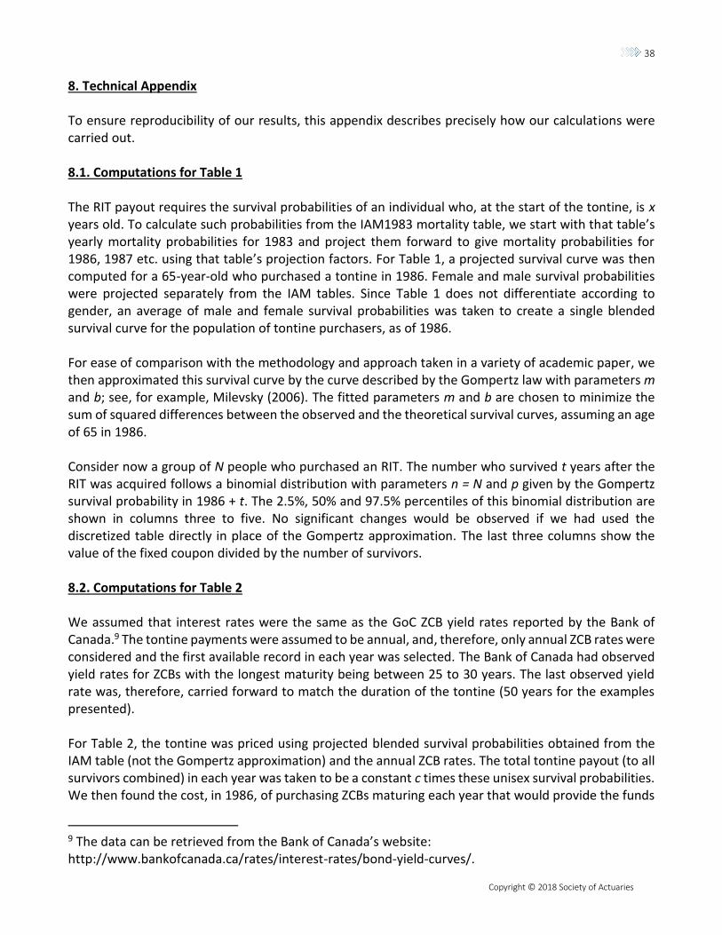
38


8. Technical Appendix To ensure reproducibility of our results, this appendix describes precisely how our calculations were carried out. 8.1. Computations for Table 1 The RIT payout requires the survival probabilities of an individual who, at the start of the tontine, is x years old. To calculate such probabilities from the IAM1983 mortality table, we start with that table’s yearly mortality probabilities for 1983 and project them forward to give mortality probabilities for 1986, 1987 etc. using that table’s projection factors. For Table 1, a projected survival curve was then computed for a 65-year-old who purchased a tontine in 1986. Female and male survival probabilities were projected separately from the IAM tables. Since Table 1 does not differentiate according to gender, an average of male and female survival probabilities was taken to create a single blended survival curve for the population of tontine purchasers, as of 1986. For ease of comparison with the methodology and approach taken in a variety of academic paper, we then approximated this survival curve by the curve described by the Gompertz law with parameters m and b; see, for example, Milevsky (2006). The fitted parameters m and b are chosen to minimize the sum of squared differences between the observed and the theoretical survival curves, assuming an age of 65 in 1986. Consider now a group of N people who purchased an RIT. The number who survived t years after the RIT was acquired follows a binomial distribution with parameters n = N and p given by the Gompertz survival probability in 1986 + t. The 2.5%, 50% and 97.5% percentiles of this binomial distribution are shown in columns three to five. No significant changes would be observed if we had used the discretized table directly in place of the Gompertz approximation. The last three columns show the value of the fixed coupon divided by the number of survivors. 8.2. Computations for Table 2 We assumed that interest rates were the same as the GoC ZCB yield rates reported by the Bank of Canada.9 The tontine payments were assumed to be annual, and, therefore, only annual ZCB rates were considered and the first available record in each year was selected. The Bank of Canada had observed yield rates for ZCBs with the longest maturity being between 25 to 30 years. The last observed yield rate was, therefore, carried forward to match the duration of the tontine (50 years for the examples presented). For Table 2, the tontine was priced using projected blended survival probabilities obtained from the IAM table (not the Gompertz approximation) and the annual ZCB rates. The total tontine payout (to all survivors combined) in each year was taken to be a constant c times these unisex survival probabilities. We then found the cost, in 1986, of purchasing ZCBs maturing each year that would provide the funds

9 The data can be retrieved from the Bank of Canada’s website: http://www.bankofcanada.ca/rates/interest-rates/bond-yield-curves/.

39


to cover these total payouts. The constant c was then chosen to ensure that the cost matched the funds available in 1986 from the contributions from the pool. The number of survivors in every year follows a binomial distribution with size parameter N and the computed survival probability. Pool sizes of N = 50, 500, 1,000 and 5,000 were considered. For all cases, the 2.5%, 50% and 97.5% percentiles from these binomial distributions were used to produce the corresponding tontine percentiles. 8.3. Computations for Table 3 For Table 3, we carried out the same calculations as above but starting the tontines in a variety of years (1986, 1987 etc.). In each case, a new survival curve was found for each initial tontine year. A distinction between males and females was now applied to price the tontine. The frequency of payments was also modified from being once a year to once a month. To deal with fractional ages and survival times, a constant force of mortality was assumed within each year. If we had used the Gompertz approximation instead of the IAM table with full projection, this interpolation would have been unnecessary. The interest rates were also modified so that the compounding frequency matched those of the tontine payments. That allowed us to compute initial tontine payouts, as described above, which are shown in Table 3a. Table 3b used these tontine structures and calculated the indicated percentiles for tontine payouts, using binomial probabilities calculated as described earlier. Table 3c and Table 3d show corresponding results from a tontine that has been backed by corporate bonds instead of government bonds. The corporate interest rates were constructed by a vertical shift in the government yield rate curve introduced in the first section. The difference between the 30-year government bond and the 30-year corporate bond (data from Scotia Capital, Bank of Canada website) determined the size of the vertical shift in the GoC ZCB curve. 8.4. Computations for Figure 1 The goal of Figure 1 is to track the path of the monthly tontine payments over 30 years. Each member of the tontine is assumed to be 65 years old in 1986, the year in which the tontine is acquired. Each curve is a simulation of successive realizations of the binomial random variables described above, repeating every month until the 30-year path was completed. A total of 1,000 paths were simulated for males and females. The horizontal lines of Figure 1 contain 95% of the tontine payments in each month. 8.5. Computations for Figure 2 Figure 2 shows a sensitivity analysis. Here the tontine parameters are calculated as in Section 3.1 with monthly payouts and for both males and females. However, in the analysis, we assume that the mortality used to price the tontine is incorrect (misspecified), and a different mortality assumption is used instead. The following describes how this different mortality assumption was chosen. Let Sm(t) and Sf(t) be the survival functions for males and females, obtained as above by fitting to the IAM1983 mortality tables. The tontine is priced using these survival probabilities. But to compute

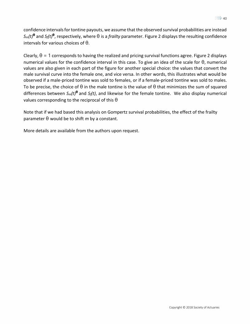
40


confidence intervals for tontine payouts, we assume that the observed survival probabilities are instead

Sm(t)θ and Sf(t)θ, respectively, where θ is a frailty parameter. Figure 2 displays the resulting confidence

intervals for various choices of θ.

Clearly, θ = 1 corresponds to having the realized and pricing survival functions agree. Figure 2 displays

numerical values for the confidence interval in this case. To give an idea of the scale for θ, numerical values are also given in each part of the figure for another special choice: the values that convert the male survival curve into the female one, and vice versa. In other words, this illustrates what would be observed if a male-priced tontine was sold to females, or if a female-priced tontine was sold to males.

To be precise, the choice of θ in the male tontine is the value of θ that minimizes the sum of squared

differences between Sm(t)θ and Sf(t), and likewise for the female tontine. We also display numerical

values corresponding to the reciprocal of this θ Note that if we had based this analysis on Gompertz survival probabilities, the effect of the frailty

parameter θ would be to shift m by a constant. More details are available from the authors upon request.

41


About The Society of Actuaries

The Society of Actuaries (SOA), formed in 1949, is one of the largest actuarial professional organizations in the world

dedicated to serving more than 27,000 actuarial members and the public in the United States, Canada and worldwide. In

line with the SOA Vision Statement, actuaries act as business leaders who develop and use mathematical models to

measure and manage risk in support of financial security for individuals, organizations and the public.

The SOA supports actuaries and advances knowledge through research and education. As part of its work, the SOA seeks to

inform public policy development and public understanding through research. The SOA aspires to be a trusted source of

objective, data-driven research and analysis with an actuarial perspective for its members, industry, policymakers and the

public. This distinct perspective comes from the SOA as an association of actuaries, who have a rigorous formal education

and direct experience as practitioners as they perform applied research. The SOA also welcomes the opportunity to partner

with other organizations in our work where appropriate.

The SOA has a history of working with public policymakers and regulators in developing historical experience studies and

projection techniques as well as individual reports on health care, retirement and other topics. The SOA’s research is

intended to aid the work of policymakers and regulators and follow certain core principles:

Objectivity: The SOA’s research informs and provides analysis that can be relied upon by other individuals or organizations

involved in public policy discussions. The SOA does not take advocacy positions or lobby specific policy proposals.

Quality: The SOA aspires to the highest ethical and quality standards in all of its research and analysis. Our research process

is overseen by experienced actuaries and nonactuaries from a range of industry sectors and organizations. A rigorous peer-

review process ensures the quality and integrity of our work.

Relevance: The SOA provides timely research on public policy issues. Our research advances actuarial knowledge while

providing critical insights on key policy issues, and thereby provides value to stakeholders and decision makers.

Quantification: The SOA leverages the diverse skill sets of actuaries to provide research and findings that are driven by the

best available data and methods. Actuaries use detailed modeling to analyze financial risk and provide distinct insight and

quantification. Further, actuarial standards require transparency and the disclosure of the assumptions and analytic

approach underlying the work.

Society of Actuaries 475 N. Martingale Road, Suite 600

Schaumburg, Illinois 60173 www.SOA.org

Annuities Versus Tontines in the 21st Century · 2018-03-07 · necessarily sell life annuities at...

Documents

Transcript of Annuities Versus Tontines in the 21st Century · 2018-03-07 · necessarily sell life annuities at...