1

Annual Report 1998 of the CODE Analysis Center of the IGS

M. Rothacher, T. Springer, G. Beutler, R. Dach, U. Hugentobler, D. Ineichen, S. SchaerAstronomical Institute, University of Bern

U. Wild, A. Wiget, E. BrockmannFederal Office of Topography, Wabern

C. BoucherInstitut Géographique National, Paris

E. Reinhart, H. HabrichBundesamt für Kartographie und Geodäsie, Frankfurt

1. Introduction

CODE, the Center for Orbit Determination in Europe, is a joint venture of- the Federal Office of Topography (L+T), Wabern, Switzerland,- the Federal Agency of Cartography and Geodesy (BKG), Frankfurt, Germany,- the Institut Géographique National (IGN), Paris, France, and- the Astronomical Institute of the University of Berne (AIUB), Berne, Switzerland.

CODE is located at the AIUB. All solutions and results are produced with thelatest version of the Bernese GPS Software [Rothacher and Mervart, 1996].

This report covers the time period from July 1998 to October 1999. It focuses onthe major changes in the routine processing during this period and shows the newdevelopments and products generated at CODE. The processing strategies used till June1998 are described in the annual reports of previous years [Rothacher et al., 1995, 1996,1997, 1998].

The rapid solution generated at CODE are based on the extended radiationpressure model [Springer et al., 1999]. The cut-off angle for all solutions is set to 10º andthe Niell mapping function [Niell, 1996] for the dry atmosphere is used. No tropospheregradients are estimated for the official global solution, gradients are determined,however, for the European as well as for some global test solutions. 1-day and 2-daypredicted Global Ionosphere Maps (GIMs) are derived regularly and delivered weekly toCDDIS. The ocean loading model according to [Scherneck, 1991] together with theocean tide maps from [Le Provost et al., 1994] is used.

For all solutions (except for the ionosphere solution) the number of stations islimited to 100. If more stations are available, those with the maximum number ofobservations are selected. Fig. 1 shows the number of stations used in the processing atCODE. Since spring 1998 usually more than 100 stations are available routinely.

2

1996 1996.5 1997 1997.5 1998 1998.5 19990

20

40

60

80

100

120

Time (years)

Num

ber

of s

tatio

ns

Figure 1: Number of stations used for the global 1-day solutions computed at CODE.

Numerous receivers in the IGS network, in particular those located near thegeomagnetic equator, severely suffer from the increasing ionospheric activity – wellbefore the next solar maximum comes within reach. Fig. 2 gives a summary of IGSreceiver performance under aggravated ionospheric conditions.

−90 −60 −30 0 30 60 900

2

4

6

8

10

Geographic latitude (degrees)

Num

ber

of s

atel

lites

−90 −60 −30 0 30 60 900

2

4

6

8

10

Geographic latitude (degrees)

Num

ber

of s

atel

lites

01:20–01:40 LT 13:20–13:40 LT

Figure 2: Average number of GPS satellites tracked by IGS receivers as a function ofgeographic latitude for 01:30 (left) and 13:30 local time (right) in September 1998.

The two figures show the average number of GPS satellites successfully trackedby the receivers as a function of geographic latitude for time intervals of 20 minutescentered around 01:30 and 13:30 local time, respectively. 'Successfully tracked' meansthat at maximum one missing measurement epoch per 20 minutes is tolerated. It isalarming to see that more or less all equatorial receivers fail to keep track of the satellitesduring the local noon hours. This is a clear indication that the problem is related to theionosphere. The problem should be taken serious because Fig. 2 does not address thesituation for a particular day but throughout the entire month of September 1998.

3

2 Changes in the CODE Routine Processing

The major changes implemented in the CODE routine analysis since July 1998are listed in Table 1. Modifications prior to this date have already been reported in lastyear’s annual report of last year [Rothacher et al. 1998].

Table 1: Modification of processing scheme at the CODE Analysis Center from July1998 to October 1999.

Date Doy/Year Description of Change, Impact16-Jul-98 187/98 New IGS ERP Format activated (version 2).20-Aug-98 232/98 Rapid solution now run using the new radiation pressure

model [Springer et al., 1999].27-Aug-98 239/98 Max degree/order of spherical harmonic expansion for

TEC/differential code biases (DCB) solution increased from3/3 to 4/4, i.e., 25 instead of 16 TEC parameters areestimated per station-day.

04-Oct-98 277/98 New normal equation stacking routine (ADDNEQ) officiallyused. Final orbits are now based on backsubstitutedcoordinates and ERP from 7-day (7 3-day) ADDNEQcombination of coordinates and ERPs.

29-Nov-98 333/98 Change of antenna offsets from 1.0259 to 1.0230 for theBlock II/IIA and from 1.2053 to 0.0000 for the Block IIR.

20-Mar-99 079/99 GIM Zero-differences used as new official CODE TECproduct. New TEC product submitted to CDDIS.

05-Apr-99 095/99 Rapid ionosphere product (including DCB estimates) isderived from zero differences. Station-specific TEC modelsbased on double differences are generated to improve QIFambiguity resolution.

11-Apr-99 101/99 All available stations are used to derive the final ionosphereproduct (Z1 solution). For the station-specific TEC maps andDCBs (Z1N solution), up to 100 station are used. For thisreason, the maximum degree of the spherical harmonicexpansion was reduced from 4 to 3.

04-Jul-99 185/99 New receiver and antenna names used.01-Aug-99 213/99 Switch to ITRF97. The new set of reference stations consists

of about 50 stations. The complete ERP time series, goingback to day 200 of 1993, was recomputed using ITRF97coordinates and velocities (see IGS Mail 2422).

24-Aug-99 236/99 Download also GZ RINEX observation files from JPL dataarchive if necessary.

26-Sep-99 269/99 12 new sites added: ARTU, BAKO, CORD, DAEJ, KUNM,PIMO, RIOG, RIOP, SYOG, URUM, YKRO, YSSK. ForRIOP and SYOG no data is currently available.

4

3. Product Quality and Results

3.1 Ionosphere

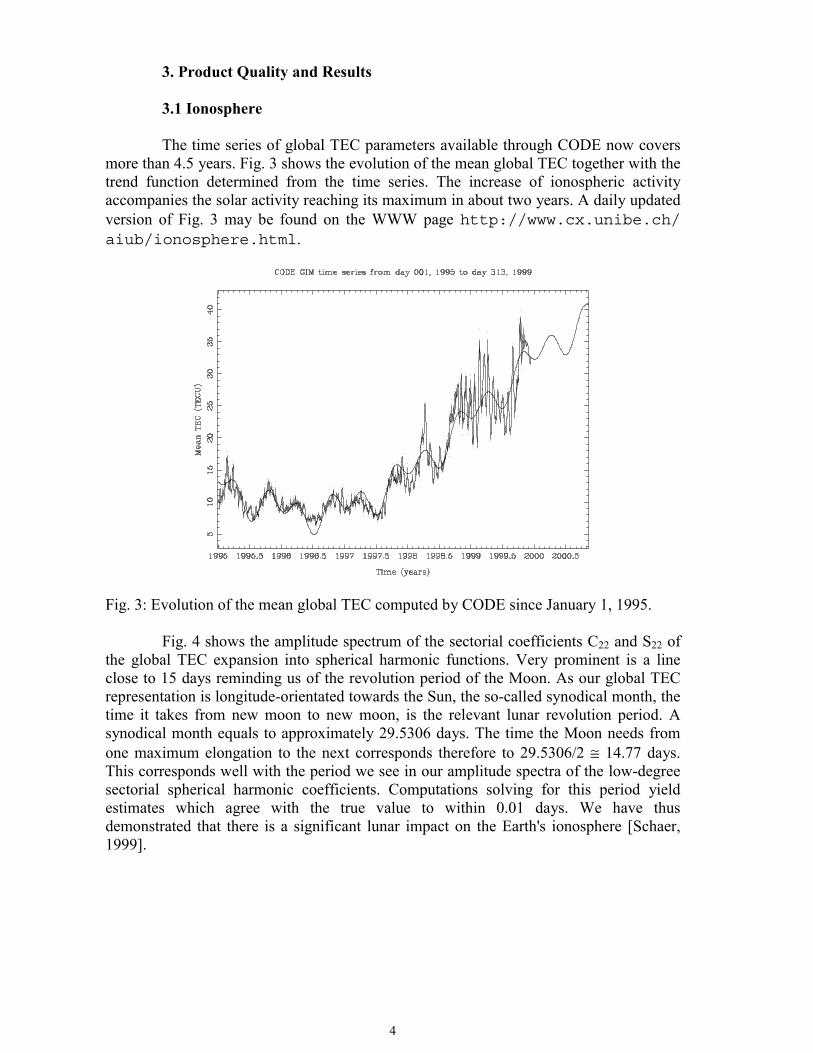
The time series of global TEC parameters available through CODE now coversmore than 4.5 years. Fig. 3 shows the evolution of the mean global TEC together with thetrend function determined from the time series. The increase of ionospheric activityaccompanies the solar activity reaching its maximum in about two years. A daily updatedversion of Fig. 3 may be found on the WWW page http://www.cx.unibe.ch/aiub/ionosphere.html.

Fig. 3: Evolution of the mean global TEC computed by CODE since January 1, 1995.

Fig. 4 shows the amplitude spectrum of the sectorial coefficients C22 and S22 ofthe global TEC expansion into spherical harmonic functions. Very prominent is a lineclose to 15 days reminding us of the revolution period of the Moon. As our global TECrepresentation is longitude-orientated towards the Sun, the so-called synodical month, thetime it takes from new moon to new moon, is the relevant lunar revolution period. Asynodical month equals to approximately 29.5306 days. The time the Moon needs fromone maximum elongation to the next corresponds therefore to 29.5306/2 ≅ 14.77 days.This corresponds well with the period we see in our amplitude spectra of the low-degreesectorial spherical harmonic coefficients. Computations solving for this period yieldestimates which agree with the true value to within 0.01 days. We have thusdemonstrated that there is a significant lunar impact on the Earth's ionosphere [Schaer,1999].

5

0 5 10 15 20 25 30 35 400

0.1

0.2

0.3

Period (days)A

mpl

itude

(T

EC

U)

0 5 10 15 20 25 30 35 400

0.1

0.2

0.3

Period (days)

Am

plitu

de (

TE

CU

)

Figure 4: Amplitude spectra of the sectorial spherical harmonic coefficients C22 (top) andS22 (bottom) for periods below 40 days.

These perturbations are probably indirectly caused by atmospheric pressurevariations associated with lunar gravitational tides as postulated by [Rishbeth andGarriott, 1969]. These tidal waves, considered in an Earth-fixed frame, respond to thewell-known tidal cycle of about 12 hours 25 minutes. Another piece of evidence has to beseen in the fact that the influence of the Moon on the ionosphere is not only confirmed bythe particular period of 14.77 days but also by the coefficient-specific phases themselves,which are in agreement with the lunation cycle. Small phase shifts offer a basis forfurther investigations.

3.2 Earth Rotation Parameters

In April 1994 CODE started to estimate nutation rate corrections in longitudeand obliquity relative to the IAU 1980 theory of nutation (which is used as a priori modelin our processing). The series of nutation rate estimates covers by now a time interval ofmore than 5 years. Results of a detailed analysis of the time series was presented at theIGS Analysis Workshop in Darmstadt, 1998 [Rothacher and Beutler, 1998]. They showthat GPS may give a significant contribution to nutation in the high frequency range ofthe spetrum (periods below 20 days). The nutation coefficients estimated from GPS rateseries show an overall agreement of about 10 µas with the most recent nutation modelsby Souchay and Kinoshita [Rothacher et al., 1999].

Internally, CODE uses a 2-hour resolution since January 1995 to account forpolar motion and LOD. Each component of this high-resolution polar motion series (andthe corresponding integrated LOD series) is approximated by a linear function withineach 2-hour sub-interval and continuity is enforced at the interval boundaries. The sub-

6

daily variations of polar motion and UT correspond very well to models derived fromoceanography using altimetry data.

Fig. 5 shows the amplitude spectrum of the diurnal and semi-diurnal tidalfrequency bands for UT1 generated from the sub-daily ERP series. The noise level is ofthe order of 0.5-1.0 µs which enables us to clearly see all the major tidal terms. Thespectra of these GPS series demonstrate the potential of the technique. The series is stillfar too short, however, to give insight into the sidebands of the major tides. For moredetails we refer to [Rothacher, 1998].

Diurnal UT1 Semi-diurnal UT1

Figure 5: Amplitude spectra of the diurnal and semi-diurnal tidal frequency bandsgenerated from the entire sub-daily ERP series. The major tidal terms are labeled. Thespectra were computed from the UT1 rate estimates and subsequently converted tospectra in UT1.

3.3 Orbit Validation using SLR

The SLR observations of the GPS (and GLONASS) satellites provide a uniqueopportunity to validate the quality of the IGS (and IGEX) orbit determination using anindependent method. For a comparison all observations acquired by 25 SLR stations tothe two GPS satellites PRN 5 and PRN 6, that are equipped with retroreflectors were used[Springer, 1999]. The SLR station positions were taken from the ITRF realization, thesatellite orbits from the CODE analysis center. The tropospheric delays are modeledusing the Marini-Murray model [Marini et al., 1973].

Figure 6 shows the differences between the observed and computed ranges usingall SLR observations of the GPS satellites over the time span from January 1995 to July1999. Outliers were removed using a 5σ outlier criterium.

Two interesting results emerge from Fig. 6: First, we see an average bias of –55mm between the observed and computed ranges. The negative sign indicates that theobserved SLR ranges are shorter than the computed ranges. A range bias of similarmagnitude and the same sign is observed also for GLONASS satellites [Springer, 1999].The occurrence of this bias is unexpected and asks for explanations.

7

Figure 6: Range residuals of the SLR observations from GPS satellites PRN 5 (crosses)and PRN 6 (triangles).

Secondly, the RMS of the residuals, around the mean, is as low as 55 mm. Thisresult implies that the two independent techniques, microwave and SLR, agree at thelevel of a few centimeters. Most importantly it also shows that the (radial) orbit error ofthe IGS orbits is at maximum as small as 55 mm. This corresponds quite well to the RMSstatistics of the weekly IGS orbit combinations. On the other hand, the 55 mm RMS iswell above the noise level of the SLR normal point observations.

Intensive tests to routinely combine GPS and SLR observations for thegeneration of the CODE products were carried out. The impact on the GPS-only results issmall, however, because of the sparseness of SLR data. No obvious improvements couldbe observed. For more details we refer to [Springer, 1999].

3.4 GLONASS Processing

On October 19, 1998, at the beginning of the International GLONASSExperiment (IGEX-98) [Slater et al., 1999], CODE started to compute precise orbits forall active GLONASS satellites. The processing of the IGEX network is done on a routinebasis and precise ephemerides are made available through the global IGEX Data Centers.For the combined processing of GLONASS and GPS data the enhanced Version 4.1 ofthe Bernese GPS Software is used [Rothacher and Mervart, 1996, Habrich 1999].

The analysis is done by fixing both, the GPS orbits and Earth rotationparameters to CODE's final IGS solution. The number of available sites within the IGEXnetwork (about 35 sites) would not allow to estimate these parameters with an accuracycomparable to the IGS solutions. The orbital parameters of the GLONASS satellites areestimated using double difference phase observations (including double differencesbetween GLONASS and GPS satellites). The processing of the IGEX network is donewithout fixing the ambiguities to their integer values.

8

Six initial conditions and nine radiation pressure parameters are determined foreach satellite and arc. So far only receivers providing dual-frequency GPS andGLONASS data or dual frequency GLONASS data are included in the processingprocedure. The final precise orbits stem from the middle day of a 5-day arc. In order toalign the IGEX network to the terrestial reference frame the coordinates of seven sites areconstrained to their ITRF 96 coordinates [Ineichen et al., 1999].

In order to check the internal consistency of our GLONASS orbits, we perform along-arc fit for each processed week. For each satellite, one orbital arc is fitted throughthe seven consecutive daily solutions of the week. The RMS values lie in general between5 and 20 cm. These small values indicate that the adopted orbit model is well suited todescribe the motion of the GLONASS satellites over a time period of several days. Anindependent check of the orbit accuracy is given by the range residuals of SLRobservations showing a RMS of 13 cm [Springer, 1999].

The difference between the GLONASS and GPS system times was set up as oneadditional parameter for each station and session. The results show that this time systemdifference is receiver dependent. Fig. 7 shows the estimated system time difference forthe Z18 (upper band) and the JPS receivers (lower two bands). The time differences forother receivers are of the order of one microsecond.

Figure 7: Differences between GPS and GLONASS system times for Z18 (upper band)and JPS receivers (lower two bands).

GPS and GLONASS broadcast orbits are given in different reference systems.The seven parameters of a Helmert transformation were determined using preciseGLONASS orbits in the ITRF 96 reference frame and the broadcast GLONASS orbits inthe PZ-90 reference frame. For each day one set of parameters (three translations, threerotations, and one scale factor) was established. The accuracy of the daily Helmerttransformations (RMS between 3 m and 6 m) indicate the GLONASS broadcast orbitquality.

Fig. 8 shows the time series of the rotation parameters. A rotation of –350 masaround the z-axis is found to be highly significant and has to be taken into account whenprocessing combined GLONASS and GPS data using broadcast orbits. The values of theother rotation parameters as well as the translation and scale parameters are limited by thebroadcast orbit accuracy.

9

Figure 8: Daily rotation parameters of the Helmert transformation between broadcastorbits in the PZ-90 system and CODE's precise orbits in the ITRF 96 system.

3.5 Time and Frequency Transfer using GPS

In 1991 a common project of the Federal Office of Metrology (EAM) andCODE/AIUB was initiated to develop time transfer terminals based on geodetic GPSreceivers. The goal is the comparison of time scales with sub-nanosecond accuracy andfrequencies with an accuracy of 10-15 over one day for two or more (GPS-external)clocks.

Three prototype Geodetic Time Transfer terminals (GeTT terminals) weredeveloped. They are based on modified Ashtech Z-12 receivers installed in a temperaturecontrolled container. More information about the time transfer project and the GeTTterminals may be found in [Schildknecht et al., 1990, Overney et al., 1998, Dudle et al.,1999].

After careful calibration of delays in cables, temperature-dependent delays, etc.,two GeTT terminals were deployed on two European baselines (EAM-NPL, PTB-NPL(UK)). Since July 1998 two terminals are located in the time laboratories of PTB inBraunschweig, Germany, and USNO in Washington, USA, on an intercontinentalbaseline with a length of 6'275 km. In both laboratories other time transfer equipment isavailable, such as GPS Common View (GPS-CV) or Two Way Satellite Time andFrequency Transfer (TWSTFT) allowing a comparison with the geodetic time transfermethod on the sub-nanosecond level.

The data from a permanent time and frequency comparison network is processedroutinely at CODE using the zero differencing capability of the Bernese GPS Softwareand using the IGS final products such as precise orbits, troposphere and ionosphereparameters. In Fig. 9 the time difference between PTB and USNO is shown as measuredby GeTT, TWSTFT, and Circular T, the official difference determined by the BureauInternational des Poids et Mesures (BIPM) based on GPS-CV which relies on pure GPScode measurements. Fig. 10 shows the difference between the GeTT and the TWSTFTmeasurements. The reason for the systematic variations of the difference between the twomethods is not yet understood and is discussed within the time transfer community. It hasto be pointed out that accuracy-wise, geodetic time transfer with GPS is the only methodcompeting with TWSTFT on intercontinental baselines.

10

-80

-60

-40

-20

0

20

40

60

80

∆ Clo

ck in

ns

51050 51100 51150 51200 51250 51300 51350

MJD

GeTT GPS phase measurement

Circular T values

TWSTFT values

Figure 9: Time difference between reference clocks at PTB, Braunschweig, Germany,and USNO, Washington, USA, as measured by geodetic GPS (GeTT) and Two WaySatellite Time and Frequency Transfer (TWSFTF), together with the values from CircularT published by the Bureau International des Poids et Mesures (BIPM). The offsetsbetween the different measurements are arbitrary.

-5

-4

-3

-2

-1

0

1

2

3

4

5

∆ Clo

ck in

ns

51050 51100 51150 51200 51250 51300 51350

MJD

Figure 10: Difference between the clock differences between PTB and USNO asmeasured by geodetic GPS (GeTT) and TWSTFT. The systematic variation of thedifference between the two methods is not yet understood.

4 Outlook

A number of questions have to be studied in more detail in the near future suchas the correlation between satellite antenna phase centers, troposphere, and GPS scale;and the ‘y-shift’ of the geocenter observed when introducing stochastic parameters for theorbit modeling [Springer, 1999]. For the European solutions the cut-off angle is set to 5ºand troposphere gradients are estimated. The corresponding time series cover alreadyseveral years. The goal is to implement these changes for the global solutions. We areaiming at integrating the routine IGEX solution into our IGS solution. Following thetrend to generate ultra-rapid solutions we intend to replace the rapid solution by an ultra-rapid solution at some point in the future.

11

5 References

Dudle, G., F. Overney, T. Schildknecht, T. Springer, L. Prost (1999), Transatlantic Timeand Frequency Transfer by GPS Carrier Phase, in Proceedings of the 13th EuropeanFrequency and Time Forum and 1999 IEEE Internatioonal Frequency ControlSymposium, Besançon, April 13-16, 1999.

Ineichen, D., M. Rothacher, T. Springer, G. Beutler (1999), Computation of PreciseGlonass Orbits for IGEX-98, in Proceedings of the XXII General Assembly of theIUGG, Birmingham, UK, July 19-30, 1999.

Habrich, H. (1999), Geodetic Applications of the Global Navigation Satellite System(GLONASS) and of GLONASS/GPS Combinations, Ph.D. Thesis, Druckerei derUniversität Bern, Bern.

Le Provost, C., M. L. Genco, F. Lyard, P. Vincent, P. Canceil (1994), Spectroscopy of theworld ocean tides from a finite element hydrodynamic model, JGR, 99, pp. 24777-24797.

Marini, J.W., and C.W. Murray (1973), Correction of Laser Range Tracking Data forAtmospheric Refraction at Elevations Above 10 Degrees, X-591-73-351, NASAGSFC.

Niell, A.E. (1996), Global Mapping Functions for the Atmosphere Delay at RadioWavelengths, JGR, 101, B2, pp. 3227-3246.

Overney, F., L. Prost, G. Dudle, T. Schildknecht, G. Beutler, J.A. Davis, J.M. Furlong, P.Hetzel (1998), GPS Time Transfer Using Geodetic Receivers (GeTT): Results onEuropean Baselines, in Proceedings of the 12th European Frequency and Time ForumEFTF 98, Warsaw, Poland, March 10-12.

Rishbeth, H., O.K. Garriott (1969), Introduction to Ionospheric Physics, Vol. 14 ofInternational Geophysics Series.

Rothacher, M., G. Beutler, E. Brockmann, L. Mervart, R. Weber, U. Wild, A. Wiget, H.Seeger, S. Botton, C. Boucher (1995), Annual Report 1994 of the CODE ProcessingCenter of the IGS, in IGS 1994 Annual Report, edited by J.F. Zumberge et al., pp. 139-162, Central Bureau, JPL, Pasadena, CA.

Rothacher, M., G. Beutler, E. Brockmann, L. Mervart, S. Schaer, T.A. Springer, U. Wild,A. Wiget, H. Seeger, C. Boucher (1996), Annual Report 1995 of the CODEProcessing Center of the IGS, in IGS 1995 Annual Report, edited by J.F. Zumberge etal., pp. 151-174, IGS Central Bureau, JPL, Pasadena, CA.

Rothacher, M., L. Mervart (1996), The Bernese GPS Software Version 4.0, AstronomicalInstitute, University of Berne, September, 1996.

12

Rothacher, M., T.A. Springer, S. Schaer, G. Beutler, E. Brockmann, U. Wild, A. Wiget,C. Boucher, S. Botton, H. Seeger (1997), Annual Report 1996 of the CODEProcessing Center of the IGS, in IGS 1996 Annual Report, edited by J.F. Zumberge etal., pp. 201-219, IGS Central Bureau, JPL, Pasadena, CA.

Rothacher, M. (1998), Recent Contributions of GPS to Earth Rotation and ReferenceFrames, Habilitationsschrift der philosophisch-naturwissenschaftlichen Fakultät derUniversität Bern, Druckerei der Universität Bern, Bern, 1998.

Rothacher, M., T.A. Springer, S. Schaer, G. Beutler, D. Ineichen, U. Wild, A. Wiget, C.Boucher, S. Botton, H. Seeger (1998), Annual Report 1996 of the CODE ProcessingCenter of the IGS, in IGS 1997 Annual Report, edited by J.F. Zumberge et al., pp. 73-87, IGS Central Bureau, JPL, Pasadena, CA.

Rothacher, M., G. Beutler (1998), Estimation of Nutation Terms Using GPS, inProceedings of the IGS Analysis Center Workshop, Darmstadt, February 9-11, 1998,edited by J.M. Dow et al., pp. 183-190, ESA/ESOC, Darmstadt.

Rothacher, M., G. Beutler, T. A. Herring, R. Weber (1999), Estimation of nutation usingthe Global Positioning System, JGR, 104 (B3), 4835-4859.

Schaer, S. (1999), Mapping an Predicting the Earth's Ionosphere Using the GlobalPositioning System, Geodätische-geophysikalische Arbeiten in der Schweiz,Schweizerische Geodätische Kommission, 59, Druckerei E. Zingg, Zürich, 1999.

Scherneck, H.-G. (1991), A parametrized solid earth tide model and ocean tide loadingeffects for global geodetic baseline measurements, Geophys. J. Int.,106, pp. 677-694.

Schildknecht, T., G. Beutler, W. Gurtner, M. Rothacher (1990), Towards SubnanosecondGPS Time Transfer using Geodetic Processing Techniques, in Proceedings of theFourth European Frequency and Time Forum, pp. 335-346, Neuchâtel, Switzerland.

Slater, J.A., P. Willis, G. Beutler, W. Gurtner, W. Lewandowski, C. Noll, R. Weber, R.Neilan, G. Hein, (1999). The International GLONASS Experiment (IGEX-98):Organization, Preliminary Results and Future Plans, in Proceedings of the ION GPS-99, Nashville, Sept. 14-17, 1999.

Springer, T., G. Beutler, M. Rothacher (1999), Improving the Orbit Estimates of GPSSatellites, Journal of Geodesy, 73, pp. 147-157.

Springer, T., G. Beutler, M. Rothacher (1999), A new Solar Radiation Pressure Model forGPS, Adv. Space Res., 23, No. 4, pp. 673-679.

Springer, T. (1999), Modeling and Validating Orbits and Clocks Using the GPS, Ph.D.Thesis, Druckerei der Universität Bern, Bern.