Announcements Computer Vision I
6
1 CS252A, Fall 2009 Computer Vision I Visual Tracking Computer Vision I CSE252A Lecture 19 CS252A, Fall 2009 Computer Vision I Announcements • HW 4: Due Friday, 12/4 • Final Exam: Friday, 12/11 7:00-10:00PM CS252A, Fall 2009 Computer Vision I Main tracking notions • State: usually a finite number of parameters (a vector) that characterizes the “state” (e.g., location, size, pose, deformation of thing being tracked. • Dynamics: How does the state change over time? How is that changed constrained? • Representation: How do you represent the thing being tracked • Prediction: Given the state at time t-1, what is an estimate of the state at time t? • Correction: Given the predicted state at time t, and a measurement at time t, update the state. • Initialization – what is the state at time t=0? CS252A, Fall 2009 Computer Vision I What is state? • 2-D image location, Φ=(u,v) • Image location + scale Φ=(u,v,s) • Image location + scale + orientation Φ=(u,v,s,θ) • Affine transformation • 3-D pose • 3-D pose plus internal shape parameters (some may be discrete). – e.g., for a face, 3-D pose +facial expression using FACS + eye state (open/closed). • Collections of control points specifying a spline • Above, but for multiple objects (e.g. tracking a formation of airplanes). • Augment above with temporal derivatives CS252A, Fall 2009 Computer Vision I State Examples: – object is ball, state is 3D position+velocity, measurements are stereo pairs – object is person, state is body configuration, measurements are frames – What is state here? CS252A, Fall 2009 Computer Vision I Track by detection • Assume – a very reliable detector (e.g. faces; back of heads) – detections that are well spaced in images (or have distinctive properties) e.g. news anchors; heads in public • Link detects across time – only one – easy – multiple - weighted bipartite matching
Transcript of Announcements Computer Vision I

1
CS252A, Fall 2009 Computer Vision I
Visual Tracking
Computer Vision I CSE252A Lecture 19
CS252A, Fall 2009 Computer Vision I
Announcements • HW 4: Due Friday, 12/4 • Final Exam: Friday, 12/11 7:00-10:00PM
CS252A, Fall 2009 Computer Vision I
Main tracking notions • State: usually a finite number of parameters (a
vector) that characterizes the “state” (e.g., location, size, pose, deformation of thing being tracked.
• Dynamics: How does the state change over time? How is that changed constrained?
• Representation: How do you represent the thing being tracked
• Prediction: Given the state at time t-1, what is an estimate of the state at time t?
• Correction: Given the predicted state at time t, and a measurement at time t, update the state.
• Initialization – what is the state at time t=0?
CS252A, Fall 2009 Computer Vision I
What is state? • 2-D image location, Φ=(u,v) • Image location + scale Φ=(u,v,s) • Image location + scale + orientation Φ=(u,v,s,θ) • Affine transformation • 3-D pose • 3-D pose plus internal shape parameters (some may be
discrete). – e.g., for a face, 3-D pose +facial expression using FACS + eye
state (open/closed). • Collections of control points specifying a spline • Above, but for multiple objects (e.g. tracking a formation
of airplanes). • Augment above with temporal derivatives
CS252A, Fall 2009 Computer Vision I
State Examples: – object is ball, state is 3D position+velocity,
measurements are stereo pairs – object is person, state is body configuration,
measurements are frames – What is state here?
CS252A, Fall 2009 Computer Vision I
Track by detection • Assume
– a very reliable detector (e.g. faces; back of heads)
– detections that are well spaced in images (or have distinctive properties) e.g. news anchors; heads in public
• Link detects across time – only one – easy – multiple - weighted bipartite matching
2
CS252A, Fall 2009 Computer Vision I
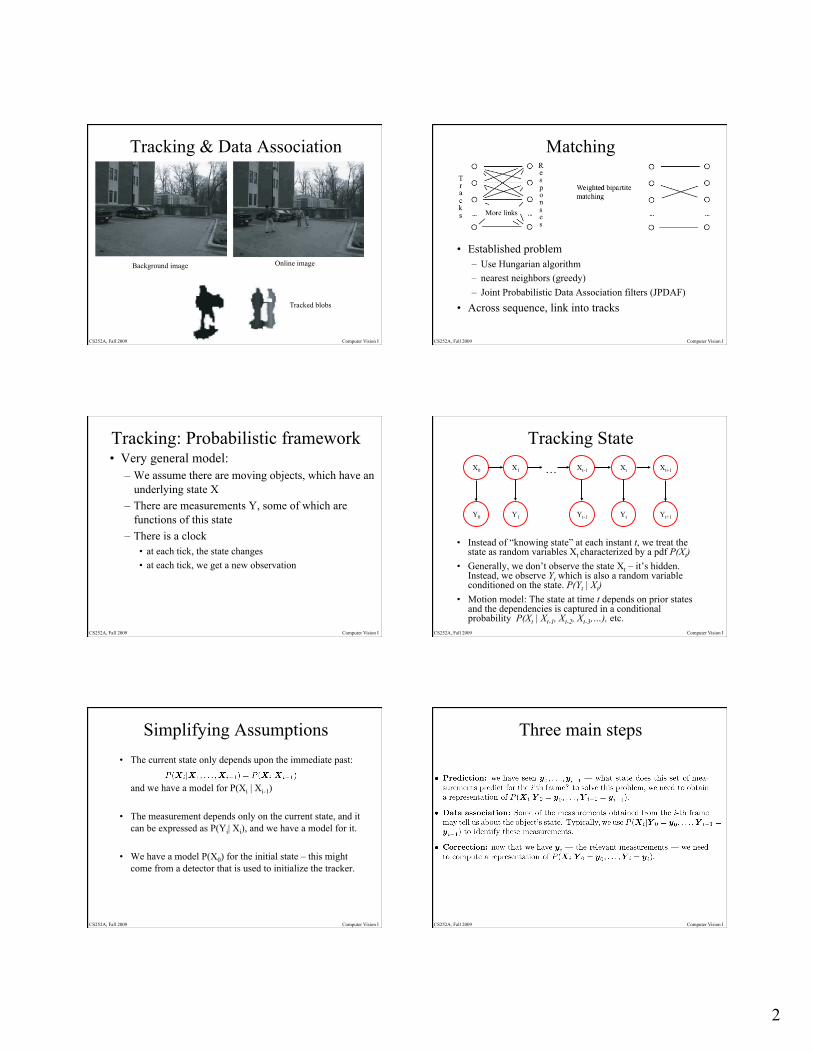
Tracking & Data Association
Background image Online image
Tracked blobs
CS252A, Fall 2009 Computer Vision I
Matching
• Established problem – Use Hungarian algorithm – nearest neighbors (greedy) – Joint Probabilistic Data Association filters (JPDAF)
• Across sequence, link into tracks
CS252A, Fall 2009 Computer Vision I
Tracking: Probabilistic framework • Very general model:
– We assume there are moving objects, which have an underlying state X
– There are measurements Y, some of which are functions of this state
– There is a clock • at each tick, the state changes • at each tick, we get a new observation
CS252A, Fall 2009 Computer Vision I
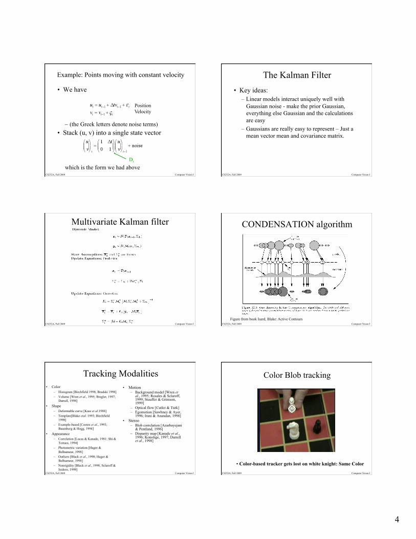
Tracking State
• Instead of “knowing state” at each instant t, we treat the state as random variables Xt characterized by a pdf P(Xt)
• Generally, we don’t observe the state Xt – it’s hidden. Instead, we observe Yt which is also a random variable conditioned on the state. P(Yt | Xt)
• Motion model: The state at time t depends on prior states and the dependencies is captured in a conditional probability P(Xt | Xt-1, Xt-2, Xt-3,…), etc.
X0 X1 Xt-1 Xt Xt+1
Y0 Y1 Yt-1 Yt Yt+1
…
CS252A, Fall 2009 Computer Vision I
Simplifying Assumptions • The current state only depends upon the immediate past:
and we have a model for P(Xi | Xi-1)
• The measurement depends only on the current state, and it can be expressed as P(Yi| Xi), and we have a model for it.
• We have a model P(X0) for the initial state – this might come from a detector that is used to initialize the tracker.
CS252A, Fall 2009 Computer Vision I
Three main steps

3
CS252A, Fall 2009 Computer Vision I
Tracking as induction • Assume data association is done
– Sometimes challenging in cluttered scenes. See work by Christopher Rasmussen on Joint Probabilistic Data Association Filters (JPDAF).
• Do correction for the 0’th frame • Assume we have corrected estimate for i’th
frame – show we can do prediction for i+1 frame,
correction for i+1 frame
CS252A, Fall 2009 Computer Vision I
Base case P(Yi | Xi) is our observation model. Given the state Xi, what is the observation. For example, P(Yi | Xi) might be a Gaussian.
Prior distribution of initial state
The Problem: Given measurement y0, what is the pdf of the state X0
Bayes Rule
CS252A, Fall 2009 Computer Vision I
Induction step: Prediction Problem: Given the result of the prior tracking step at i-1
what is the prediction P(xi | y0, …, yi-1)?
Solution: Our independence assumption makes it possible to write
CS252A, Fall 2009 Computer Vision I
Induction step: Correction Problem: Given the new measurement yi , and the prediction P(xi | y0, …, yi-1) from the previous step, what is P(Xi | y0, …, yi) ?
CS252A, Fall 2009 Computer Vision I
How is this formulation used? 1. It’s ignored. At each time instant, the
measurement is treated as the state. 2. The conditional distributions are
represented by some convenient parametric form (e.g., Gaussian).
3. The PDF’s are represented non-parametrically, and sampling techniques are used.
CS252A, Fall 2009 Computer Vision I
Linear dynamic models • Use notation ~ to mean “has the pdf of”, N(a, b)
is a multivariate normal distribution with mean a and covariance b.
• A linear dynamic model has the form
4
CS252A, Fall 2009 Computer Vision I
Example: Points moving with constant velocity
• We have
– (the Greek letters denote noise terms) • Stack (u, v) into a single state vector
which is the form we had above Di
Position Velocity
CS252A, Fall 2009 Computer Vision I
The Kalman Filter • Key ideas:
– Linear models interact uniquely well with Gaussian noise - make the prior Gaussian, everything else Gaussian and the calculations are easy
– Gaussians are really easy to represent – Just a mean vector mean and covariance matrix.
CS252A, Fall 2009 Computer Vision I
Multivariate Kalman filter
CS252A, Fall 2009 Computer Vision I
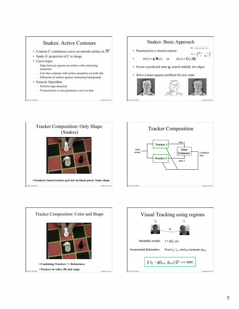
CONDENSATION algorithm
Figure from book Isard, Blake: Active Contours
CS252A, Fall 2009 Computer Vision I
Tracking Modalities • Color
– Histogram [Birchfield 1998; Bradski 1998] – Volume [Wren et al., 1995; Bregler, 1997;
Darrell, 1998] • Shape
– Deformable curve [Kass et al.1988] – Template[Blake etal. 1993; Birchfield
1998] – Example-based [Cootes et al., 1993;
Baumberg & Hogg, 1994] • Appearance
– Correlation [Lucas & Kanade, 1981; Shi & Tomasi, 1994]
– Photometric variation [Hager & Belhumeur, 1998]
– Outliers [Black et al., 1998; Hager & Belhumeur, 1998]
– Nonrigidity [Black et al., 1998; Sclaroff & Isidoro, 1998]
• Motion – Background model [Wren et
al., 1995; Rosales & Sclaroff, 1999; Stauffer & Grimson, 1999]
– Optical flow [Cutler & Turk] – Egomotion [Sawhney & Ayer,
1996; Irani & Anandan, 1998] • Stereo
– Blob correlation [Azarbayejani & Pentland, 1996]
– Disparity map [Kanade et al., 1996; Konolige, 1997; Darrell et al., 1998]
CS252A, Fall 2009 Computer Vision I
Color Blob tracking
• Color-based tracker gets lost on white knight: Same Color
5
CS252A, Fall 2009 Computer Vision I
Snakes: Active Contours • Contour C: continuous curve on smooth surface in • Snake S: projection of C to image • Curve types
– Edge between regions on surface with contrasting properties
– Line that contrasts with surface properties on both side – Silhouette of surface against contrasting background
• General Algorithm: – Perform edge detection – Fit parametric or non-parametric curve to data
CS252A, Fall 2009 Computer Vision I
Snakes: Basic Approach
• Parameterize a closed contour
• or
• Given a predicted state q, search radially for edges
• Solve a least squares problem for new state
CS252A, Fall 2009 Computer Vision I
Tracker Composition: Only Shape (Snakes)
• Geometry-based tracker gets lost on black pawn: Same shape
CS252A, Fall 2009 Computer Vision I
Tracker Composition
Tracker 1
Tracker 2
State Estimator Combined
state
Video stream
State 1
State 2
CS252A, Fall 2009 Computer Vision I
Tracker Composition: Color and Shape
• Combining Trackers => Robustness
• Trackers in video, IR and range CS252A, Fall 2009 Computer Vision I
Visual Tracking using regions I0 It
From I0, It+1 and pt compute Δpt+1 Incremental Estimation:
|| I0 - g(It+1, pt+1) ||2 ==> min
pt
It = g(I0, pt) Variability model:

6
CS252A, Fall 2009 Computer Vision I
Tracking using Textured Regions • Mean intensity difference between I and affine
warp of template image [Shi & Tomasi, 1994]
Template IR Tracked state Ic
CS252A, Fall 2009 Computer Vision I
Image Warping • Warping is a change of
coordinates: J(u,v) = I(f(u,v,p),g(u,v,p))
• Always prefer to warp to destination to avoid gaps
• Two interpolation schemes – nearest neighbor – bilinear
• J(u) = I(A u)
• Note that we can “unroll” the loop to avoid the matrix multiply
• For much of tracking, nearest neighbor works well
CS252A, Fall 2009 Computer Vision I
Template tracking: Planar Case u’i = A ui + d Planar Object => Affine motion model:
Warping
It = g(pt, I0)
CS252A, Fall 2009 Computer Vision I
Hager/Toyama: Tracking Cycle
• Prediction – Prior states predict new
appearance
• Image warping – Generate a “normalized view”
• Model inverse – Compute error from nominal
• State integration – Apply correction to state
Model Inverse
Image Warping
Δp
p
-
Reference
CS252A, Fall 2009 Computer Vision I
SSD Tracking
CS252A, Fall 2009 Computer Vision I
XVision: A tracking System
Face
Eyes Mouth
Eye Eye
BestSSD BestSSD
BestSSD
Image Processing
Composition of Primitive Trackers