ANNALS OF THE UNIVERSITY OF PETRO ŞANI 2008.pdf · BRANA LILIANA SAMOIL Ă, MARIUS DANIEL MARCU,...

ISSN 1454-8518

ANNALS

OF THE UNIVERSITY OF

PETROŞANI

ELECTRICAL ENGINEERING

VOL. 10 (XXXVII)

UNIVERSITAS PUBLISHING HOUSE

PETROŞANI - ROMANIA 2008

2

ISSN 1454-8518

EDITOR OF PUBLICATION Prof.dr.eng. Ioan-Lucian BOLUNDUŢ: Email: [email protected]

ADVISORY BOARD Prof. Dr. Eng. Pop Emil - University of Petroşani, Romania; Acad. Prof. Dr. Pivnyak

Ghenadi – National mining uninersity of Ukraine; Prof. Dr. Eng. Munteanu Radu -

Tehnichal University of Cluj-Napoca, Romania; Acad. Prof. Dr. Eng. Dasic Predrag – High

Technological Technical School, Krusevac, Serbia and Montenegro, Prof. Dr. Eng. Cierpisz Stanisław – Silesian University of Technology, Poland; Prof. Dr. Eng. Bitoleanu Alexandru - University of Craiova, Romania; Prof. Dr. Eng. Păsculescu Mihai - University

of Petroşani, Romania; Prof. Dr. Eng. Coloşi Tiberiu - Tehnichal University of Cluj-Napoca,

Romania; Prof. Dr.Eng. Szabo Willibald – “Transilvania” University of Braşov, Romania;

Prof. Dr. Eng. Poanta Aron - University of Petroşani, Romania; Prof. Dr. Eng. Manolea Gheorghe - University of Craiova, Romania; Prof. Dr. Eng. Vasilievici Alexandru -

Politechnical University of Timişoara, Romania; Assoc. Prof. Dr. Dubois Daniel - University

of Liège, Belgium; Assoc. Prof. Dr.Eng. Kovács Ernö - University of Moskolc, Hungary;

Prof. Dr. Eng. Klepikov Vladimir Borisovich – National Technical University of Kharkov,

Ukraine; Prof. Dr. Eng. Truşcă Vasile - University “Politechnica” of Bucharest, Romania;

Prof. Dr. Eng. Fotău Ion - University of Petroşani, Romania, Dr. Eng. Nicoale Dan –

Dessault Systems Simulia Corp, Providence, USA, Assist. Prof. Dr. Eng Negrut Dan –

University of Wisconsin-Madison, USA

EDITORIAL BOARD Editor-in-chief: Prof. Dr. Eng. Fotău Ion University of Petroşani

Assoc.Prof. Dr.Eng Marcu Marius University of Petroşani

Associate Editors: Prof. Dr. Eng. Poanta Aron University of Petroşani

Assoc.Prof. Dr.Eng Uţu Ilie University of Petroşani

Assoc.Prof. Dr.Eng. Pătrăşcoiu Nicolae University of Petroşani

Editor Secretary: Assistant Eng. PhD Student Sochirca Bogdan University of Petroşani

Editorial office address: University of Petroşani, 20 University Street, 332006 Petroşani, Romania,

Phone: (40) 254/54.29.94; 54.25.80; 54.25.81; 54.33.82;

Fax: (40) 254/54.34.91; 54.62.38, Telex: 72524 univp, E-mail: [email protected]

This publication is with international distribution. It is sending in 28th countries.

Annals of the University of Petroşani, Electrical Engineering, 10 (2008) 3

CONTENTS EMIL POP, MONICA LEBA, VALI SIRB, ALIN BADEA, MODELING, SIMULATION

AND CONTROL FOR AN UNDERGROUND ROOF SUPPORT AS TWO ROBOTIC

ARMS …………………………………………………………………………………………..…………..5

EMIL POP, BOGDAN SOCHIRCA, MINER LAMPS MULTIPLE PARAMETERS

MONITORING SOFTWARE ……………………………………………………………….................13

EMIL POP, IOANA CAMELIA TABACARU BARBU, MONICA LEBA, THE WIND USE

FOR RENEWABLE ENERGY……………………………………………………………………….… 18

EMIL POP, MONICA LEBA, PETRE MARIAN VAMVU, SINGLE CHIP VGA VIDEO

CONTROLLER ………………………………………………………………………………………….. 27

ARON POANTA, NICOLAE NITESCU, DAN DOJCSAR, BOGDAN SOCHIRCA,

SOFTWARE FOR DESIGNING OF THE CLEARANCE AND INTERFERENCE

FITS ………………………………………………………………………………………………………..33

CAMELIA STANOI, NEW MATERIALS FOR WATER ELECTROLYSIS ……………………40

ADRIAN MARIUS TOMUŞ , NICOLAE PĂTRĂŞCOIU, VIRTUAL INSTRUMENT TO

MEASURE THE ROTATION SPEED ........................................................................................45

TITU NICULESCU, THE STUDY OF ELECTRO-DYNAMICS FORCES FOR THREE-

PHASE SHORT CIRCUITS …………………………………………………………………………….51

VIOLETA-VALI CIUCUR, APPLICATION CONSIDERATIONS — CVT ELECTRICAL

CHARACTERISTICS DURING LINEAR AND NONLINEAR LOADING ……………………..... 55

ANGELA EGRI, ADRIAN TUL BURE , VALI SARB, EMBEDDED DEVLOPMENT

ENVIROMENT TO CONTROL THE CIM-SYSTEMS……………………………………………… 61

LARISA MĂGHERUŞAN, A SHORT PRESENTATION OF THE DYE SENSITIZED

NANOSTRUCTURES SOLAR CELLS ……………………………………………………………......68

NICOLAE PĂTRĂŞCOIU, ADRIAN TOMUŞ, CECILIA ROŞULESCU, USING

THERMOCOUPLES IN PROGRAMMABLE SYSTEMS FOR MEASURING

TEMPERATURE .........................................................................................................................73

BRANA LILIANA SAMOILĂ, MARIUS DANIEL MARCU, ILIE UŢU, VISUAL BASIC

APPLICATION FOR CALCULATING THE FLOATATION FLOWSHEETS ……………….......80

CAMELIA STANOI, ALEXANDRU LAUTARU, SOLAR - HYDROGEN ENERGY…….. 84

ELENA ZBURLEA, REACTORS ……………………………………………………………………90

ANGELA EGRI, CHIVUTA-VALI SARB, ALIN BADEA, OPTICAL CHARACTER

RECOGNITION USING A MULTILAYER PERCEPTRON TYPE NEURAL NETWORK…... 102

Annals of the University of Petroşani, Electrical Engineering, 10 (2008) pages 5-12

MODELING, SIMULATION AND CONTROL FOR AN UNDERGROUND ROOF SUPPORT AS TWO ROBOTIC

ARMS

EMIL POP1, MONICA LEBA2, VALI SIRB3, ALIN BADEA4

Abstract: This paper first considers an underground roof support as two robotic arms. Based on

robotic formalism, the cinematic direct and inverse models were developed and simulated.

Based on the simulation results a software-oriented controller for the PC was designed and

implemented. The underground roof support is hardware interfaced with the PC. Using the

controller’s Graphic User Interface the overall system performances can be tested and

evaluated.

Keywords: modeling, simulation, underground support, robotic arms, software controller.

1.INTRODUCTION

In this section, the underground roof support will be considered and analyzed

in order to transform it into a two legs robot. [2]. Then, using the Denavit-Hartenberg

(D-H) formalism the homogeneous movement matrix is determined. This allows

testing the functionality of the support and developing a strategy of control based on

direct and inverse cinematic models.

1.1 GENERAL VIEW

Nowadays for the underground works like tunnel or minerals exploitations,

special machinery is used. This machinery may be designed to sustain the roof of the

works, protect the personal and other equipments and continue to move underground to

accomplish its task. Today the underground roof support has hydraulic drives with

1 Ph.D Prof Eng. at University of Petrosani

2 Ph.D Assoc Prof. Eng. at University of Petrosani

3 Ph.D Lecturer Eng at University of Petrosani

4 Ph.D Student at University of Petrosani

LEBA, M., SIRB, V., BADEA, A

6

different degrees of mobility. The most complex ones have five degrees of mobility,

four on the roof and one on the base. Fig.1 presents an underground roof support

(URS) as real view and its schematic

a) b)

Fig.1. Five grades of mobility underground support: a) Real view; b) Schematic representation

The support has two arms, one on the roof with four joints (two of these are

prismatic and two are rotation) and one at the base with only one prismatic joint.

For each arm the characteristic point is placed on the terminal element. The

two characteristic points are called RCP (Roof Characteristic Point) and FCP (Floor

Characteristic Point). The elements of the first arm are: C1 that is the main hydraulic

cylinder, C2 that is the hydraulic cylinder for the main roof beam (MRB), C3 that is the

hydraulic cylinder for the translation beam (TB) and C4 that is the hydraulic cylinder

for the peak beam (PB). The elements of the second arm are: the main floor beam

(MFB), C5 that is the hydraulic cylinder for the stepping beam (SB) and the transporter

machine (TM). The link between the two arms is made through the shield mechanism

(SM).

This underground roof support operates in six sequences as follows:

Initial position, when the TM is in the face of working, having the peak folded

and the MRB fixed on the roof.

The mining combine cut a strip from the face of working in front of the URS

and the PB is set to horizontal position.

The SB pushes the TM in the face of working.

The URS is outstretched from the roof.

The URS is moved near the TM and the PB is folded.

The URS is fixed to the roof.

MODELING, SIMULATION AND CONTROL FOR AN UNDERGROUND ROOF

SUPPORT AS TWO ROBOTIC ARMS

7

1.2. UNDERGROUND ROOF SUPPORT AS FIVE GRADES OF MOBILITY ROBOT

In this section, we represent the underground roof support as robot with five

degrees of mobility, three of these are prismatic (T) and two are rotations (R), in the

sequence TTRTR. The schematic diagram of this robot together with the appropriate

systems of coordinates for applying the D-H method is presented in fig.2.

Fig.2. Five grades of mobility two arms underground robot: a) URS schematic diagram;

b) URS upper arm; c) Upper arm D-H table; d) URS lower arm; c) Lower arm D-H table;

The equations of the robot are:

θ++++θ+θθ+θθ+θ

θ++θ+θθ+θ−θ+θ=

1000

sin)lL(hH)sin(C0)cos()sin(

cos)lL()cos(C0)sin()cos(

0100

T1212121

1212121

4,0 (1)

for the upper arm and:

++=

1000

uVU100

0010

0001

T 2,0 (2)

for the lower arm.


8

We will use the following notations:

YT – lower arm translation on y0

YG – upper arm translation and rotation on y0

ZG – upper arm translation and rotation on z0

There are obtained the direct cinematic model equations:

hHsin)lL()sin(CZ

cos)lL()cos(CY

uVUY

121G

121G

T

++θ++θ+θ=

θ++θ+θ=

++=

(3)

These equations are very important for analyzing the URS, testing and

controller design.

This approach has many advantages. First, the representation is simple and

natural. Second, the movement of the URS can be tested very easily. Third, the

equations for positioning and rotations of arms are obtained easily. On the other hand,

by this method it is possible to use the mathematical equations to model, simulate and

design the controller of URS.

1.2 MODELING AND SIMULATION

Based on equations above, in this section, there will be modeled, simulated and

tested the major performances of the URS. In fig.3 are presented the MatLab Simulink

model and simulation results for a practical case.

a)

b) Fig.3.Direct cinematic model: a) Simulation diagram; b) Simulation results



9

2. PROBLEM FORMULATION

In this section, we determine the cinematic inverse model and design the

software controller for URS, based on this model.

2.1.THE CINEMATIC INVERSE MODEL

In order to control the URS it is necessary to determine the extremity position

of the two robot arms. Based on equations (3) of the direct cinematic model, there is

determined the inverse cinematic model, as the following algorithm:

a) There are known the geometrical and technological data of the URS: H, L, U, V, C,

h, l, u;

b) There are given the RCP and FPC coordinates: YG, ZG, YT;

c) There is determined the peak rotation angle:

]0,[;)lL(C2

)lL(C)]hH(Z[Yarccos 2

222GG

2 π−∈θ+

−−−+−+=θ (4)

d) There are determined the intermediary means:

lLB

)hH(ZA G

+=

+−= (5)

e) There is determined the intermediary angle ϕ :

2222G

222G

22G

2

BCAY

])BC(AY][AY)BC[(arctg

+−+

−−+−−+=ϕ (6)

f) There is determined the roof beam rotation angle:

]2/,2/[;AY

Aarcsin 1

22G

1 ππ−∈θϕ−+

=θ (7)

2.2 SOFTWARE CONTROLLER DESIGN

The software controller must generate five appropriate signals to control the

joints. These signals can be outputted through a data acquisition card or other hardware

interface.

The control signals are grouped in a five components matrix c=(h, l, u, YG,

ZG). This will be generated automatically by a sequential controller based on a preset

program. This represents a mining dedicated PLC (fig.4).


10

Fig.4. Block diagram of the URS controller

3. PROBLEM SOLUTION

3.1 CONTROLLER SIMULINK MODEL

Using the equations of inverse model (4) - (7), there is designed the Simulink

model from fig.5.a. In fig.5.b are shown the simulation results for the case of URS

outstretched position.

Fig.5. URS controller simulation: a) Simulation model; b) Simulation result



11

3.2 THE SOFTWARE CONTROLLER AND GUI

Based on the above model, there was developed a simple algorithm that was

implemented in Visual C# programming language, as software oriented design having

the graphic user interface (GUI) presented in fig.6.

Fig.6. Graphic User Interface

In order to design the software, there was used the object oriented paradigm.

There were defined four dedicated classes, as follows:

• D3Dgraphics class, that implements methods to render the roof support, to

initialize the graphical device and to upload the graphical elements from *.x

files.

• RoofSuppElem class, that does the abstract data type for all the elements of the

roof support and has the method to render each of the elements.

• RoofSupport class, that groups all elements which form up the roof support.

This class also contains the movement constraints.

• RoofSuppInt class, that achieves the link between process and software.

The GUI has two main parts. The first, from the left side, is used to display a

3D animation. The second, right side, represents a control panel. This panel has itself

two parts. The upper side consists of several buttons that allow the user to control the

roof support, using the direct cinematic model. The lower side is the inverse cinematic

model panel. This part consists of four preset sequences, as follows: Initial Position;

Move Transporter; Advance Support; Complete Cycle.

When the user selects one of the above sequences, there are sent the

appropriate signals to move the elements of the roof support, there are displayed in a


12

special window on the GUI the sequence corresponding steps and also displayed the

peak and transporter real coordinates.

4.CONCLUSION

In this paper, there is analyzed the problem of an URS control system. For this

reason, there is considered the URS configured as a two arms robot. Each of these two

arms is analyzed using the Denavit-Hartenberg formalism. There are determined the

direct and inverse cinematic models. These models are validated using MatLab-

Simulink simulation environment. The simulation results are conform to the real roof

support.

An important problem is the design of the controller based on the inverse

models determined. The use of rigorous mathematic models allows the implementation

of complex control algorithms.

The solution can be easily implemented either on a PC or on a dedicated PLC.

REFERENCES:

[1].M.Abrudean, T.Colosi, Method for numerical modeling and simulation, Casa

Cartii de Stiinta, Cluj-Napoca, 2002.

[2]. T.Colosi, S.Codreanu, Numerical Modeling and Simulation of Dynamical

Systems, Casa Cartii de Stiinta, Cluj-Napoca, 1995.

[3]. M.Leba, E.Pop, P.Stoian, ”HIL simulation and software control of robotic arm”,

International Symposium CSCS15, Bucuresti, Romania, ISBN 973-8449-89-8, ISBN

973-8449-90-1, pp.495-500, May 2005.

[4].E.Pop, Automatizari in industria miniera, Editura Didactica si Pedagogica,

Bucuresti, 1983.

[5]. E.Pop, M.Leba and M.Pop, Sisteme de conducere a robotilor. Structura,

modelarea, simularea si conducerea robotilor ficsi si mobili, Editura Didactica si

Pedagogica, Bucuresti, 2007.

[6]. E.Pop, M.Pop, M.Leba, ”Graphic Simulation and Digital Control for Drilling

Robot”. Proceedings of Q&A-R 2000 International Conference, Cluj-Napoca,

Romania, ISBN 973-686-056-6, ISBN 973-686-058-2, pg.191-196, May 2000.

[7]. K.Watson, C.Nagel, J.H.Pedersen, J.Reid, M.Skinner, E.White, Beginning Visual

C# 2005, Wrox, ISBN: 978-0-7645-7847-2, November 2005, 1104 pg.


MINER LAMPS MULTIPLE PARAMETERS MONITORING SOFTWARE

EMIL POP1, BOGDAN SOCHIRCA2

Abstract: In this paper we propose a solution for monitoring miner lamps parameters for a

better management and to help the human factor. With the new technology that is introduced in

all aspects of life, the human factor has to be more careful to maintain those to best parameters.

This software comes to help and to provide a better and a faster management for miners lamp.

Keywords: explosive areas, miners lamp, monitoring software, Visual Basic 2005

1. INTRODUCTION

The risk area are called dangerous area- the usual staff that can create un

explosion risk are:

-crude oil;

-mineral oil and all his other products;

-natural gases;

-combustible including bio gases and those from the purifying plant;

-metal powder or organic products from the food industry;

-coal powder;

-fiber and other suspension;

It was defined a series of standard witch concern what it have to be done by the

electric equipment with have as a working area the potentially explosive areas.

-SR EN 60079-0:2005 Electrical apparatus for gas explosive atmospheres. Part 0:

General requirements

- SR EN 60079-1:2008 Electrical apparatus for explosive gas atmospheres. Part 1:

Flameproof enclosures “d”


Pressurized enclosures “p”


2 Ph.D Student Assistant Eng. at University of Petrosani

POP, E., SOCHIRCA, B.

14


Equipment protection by powder filling “q”- SR EN 60079-6:2007 Electrical apparatus

for explosive gas atmospheres. Part 6: Equipment protection by oil immersion “o”

- SR EN 60079-7:2007 Electrical apparatus for explosive gas atmospheres.Atmosfere

explozive. Part 7: Equipment protection by increased safety “e”


Equipment protection by intrinsic safety “i”

The intrinsic safety “i” it’s a technique to prevent the explosion in the

environment potentially explosive. A circuit with intrinsic safety is a circuit where any

spark or thermo effect witch it’s product in this specified product standard, witch

involved a normal condition or fault condition, is not capable to ignite an explosive gas

atmosphere, vapors or dust with air if this is present.

The intrinsic safety “i” is a low power technique forced in practice at 1W, used

usual at the industrial measure circuit. It can not be used at high power equipments, as

motors or illuminations but can be used at the circuits witch controls this.

For a device used in a potentially explosive area to be certified as a device with

intrinsic safety it is necessary as some parameters as voltage, current or power not to

pass some values, this can be achieved by interposition between the safe and the

explosive area, a certified interface.

The simple devices witch where is not necessary anti explosive protections are:

-passives components – contacts, resistors, diodes;

-good defined source witch hold safe energy;

-source witch generate energy not bigger then 1,5V and 100 mA;

-FIELDBUS system witch have their own intrinsic standards according with

EC 60079-27

2. THE PROBLEM

In this paper our purpose is to design a system witch respect the intrinsic safety

parameters. In this case it was considered the case of miner lamp type ELM 01-S/D,

lamp designed for portable individual lightning in environments with explosive

potential group 1, special designed for coal mines. Is build in conformity with

specification of EN 62013-1 and EN 62013-2 standards (fig.1).

Figure 1 Miner lamps, front and side view


15

This head lamp is designed for portable individual lighting in environments

with explosive potential. Lamp is classified in GROUP II 2B, temperature class T3

(200C), for working zone 1 with gas and fuel dusts.

Have 2 distinctive parts - battery and head-lamp connected by a cable. The

battery is made by 3 dried cells type R 20, protection degree IP 54. Material for

battery case is polycarbonate, a very resistant material to working conditions. This

material is not charging electrostatic. At the inside of the head lamp is an electronic

equipment based on a micro-controller with multi functions generated by a software. It

use 1 Luxeon Star LED at 1W as main light source. The cables have flexible wires and

a rope for resistance. Lamp is equipped with protection for short-circuit, over-charge

and thermal protection. All those protections are inside battery case. Mining head-lamp

is an EEx I lamp designed for environments with explosive potential GROUP I, build

according with specifications of EN 62013-1 and EN 62013-2 standards.

The battery type is a NiMh, 7Ah capacity and the nominal tension of 3.75V

with a life time of 800 cycles.

3.THE SOLUTION

The software designed is for helping the maintenance of the miners lamps that

we described above, with the involvement of the life expectation of the battery.

The communication between the lamp and the computer is made by serial port.

As soon as you run the program you have the possibility to chose the communication

port. After the selection of the port we can chose the desired rack that we want to

interrogate. The maximum number of the rack is 32 and the maximum number of the

lamps on the rack is 102 (figure 2)

Figure 2. Selection of the rack

POP, E., SOCHIRCA, B.

16

After the selection of the rack it will appear a new window where we will see

the number of the lamps and a series of important date regarding each lamp.

Each lamp have an unique identification number obtained after an internal

algorithm implemented in the moment when the microcontroller was programmed.

This code can not be found in two microcontrollers.

When the START button is pressed, the software start with interrogation of the

lamps. The maximum time allocated for each lamp is 2 second, so a rack can be

interrogated in 2-3 minutes depending of the state of the lamps and number of the

lamps.(figure 3)

Figure 3. The main window

For each lamp is allocated an array of controls by example an progress bar

witch illustrate graphic the charge level for the accumulator, an identification number

and a check box witch is used in case that we want to deep discharge the battery,

operation recommended by the producer to be used after 30 complete cycles for a

longer life of the accumulator.

For each lamp is displayed (as we can see in figure 3) the type of the lamp (the

software can recognized many types of lamps), the remaining time until the lamp is

fully charged (expressed in seconds, minutes, hours). If the lamp is in the charging

state the progress bar will be green and if the lamp is in the deep discharge state the

progress bar will be blue. Also for each lamp is showed the serial number, the

production date, the voltage for the accumulator, the total number of cycles (the

accumulator if is properly maintain can be up to 800).


17

Also the software is linked to a access database and for each lamp (the serial

number of the lamp is the identification key) can be stored different date. The user

have 4 fields: the user of the lamp name, serial lamp (is different of the internal serial,

this one can be write by each owner), an observation field and a special field. All those

fields can be used by the owner.

When a lamb reach the 30 cycles it will signalize that the lamp need a deep

discharge and will mark it. When it is pushed the DEEP DESCGARGE button then all

the marked lamp will start automatically start discharging. If a lamp that is marked for

a deep discharge, the operator didn’t want to discharge the is enough just to unmark it

and the software will not discharge that lamp.

3. CONCLUSIONS

In the miner process in Valea Jiului and not only there, it can be observed an

modernization and a retechnologization of work , requirements imposed by the

existing standards for a better course of the technologic process.

The classics miner lamps was replaced with success at almost all mines with

the new generation of lamps based on the LED technologies controlled by

microcontrollers, with a weight lower then the old one, but with superiors performance.

The software it is designate for the maintenance of the new generation of

miner lamps, making the life of exploitation longer.

REFERENCES

[1]. Andrew T., - Pro VB 2005 and .NET 2.0 platform, Editura Apress, U.S.A., 2006 [2]. Boehm A., - Murach’s ADO.NET 2.0 database programming with VB 2005, Editura Murach, U.S.A., 2005 [3]. Pop E., Leba M., - Microcontrollere şi automate programabile, Editura Didactică şi Pedagogică, Bucureşti 2003. [4]. Pop E., - Automatizări în industria minieră, Editura Didactică şi Pedagogică, Bucureşti 1983 [5]. Pop E., Leba M., - Proiectarea cu VLSI o alternativa pentru realizarea echipamentleor de automatizare antiexplozive cu siguranţă intrinsecă, Proceedings of the international symposium SESAM, INSEMEX, România, ISBN 973-677-047-8, pp. 154-159, 2005


THE WIND USE FOR RENEWABLE ENERGY

EMIL POP1, IOANA CAMELIA TABACARU BARBU2,MONICA

LEBA3,

Abstract: The knowledge of wind forming process, atmospheric dynamic equations and

atmospheric movements can be a real help for a better understanding of the wind as a renewable

energetic resource. The wind is one of the main energetic renewable resources. In this paper are

analyzed many problems: wind forming process, energetic balance, local and regional winds. At

the end of paper, based on these problems, is presented a simplified model of mountain, valley,

sea and land breezes.

Keywords: Renewable energy, wind process, energetic balance, global winds

1. WIND FORMING IN THE ATMOSPHERE Earth atmosphere is a gases mixture. In a volume close to Earth surface we

have 78% nitrogen and 21% oxygen. The water vapors can condense in liquid particles

of clouds or can be transformed in delicate ice crystals. The water is the only substance

from our atmosphere which can be find in three natural states like gas (water vapors),

liquid (water) and solid (ice). Both water vapors and carbon dioxide are important

greenhouse gases.

The atmospheric pressure at any level represents the total mass of the air above

this level; atmospheric pressure is decreasing with height increasing. The atmosphere

can be divided in levels according to the vertical profile of the temperature, the gases

compositions and the electrical properties.

The Earth is spinning around the Sun with 107172 km/h medium speed and in

the same time is spinning with 16736 km/h at the Equator around is own. Because of

these movements and because of the solar radiation which falk on the oblique planet

we have seasons. But the solar energy is not uniform distributed across the Earth, so

1 Ph.D. Professor at University of Petrosani

2 Ph.D Assistant at University of Petrosani

3 Ph.D.Associated Professor at University of Petrosani

POP, E., BARBU, C., LEBA, B.

19

tropical areas get more energy then polar areas. This lack of balance leads our

atmosphere through dynamical patterns of wind and weather.

The atmosphere has internal energy which is the total amount of the stored

energy in its molecules. The heat, on the other hand is the energy which is transferred

from an object to the other because of temperature difference between them. After the

transfer of heat, that heat is stored as internal energy. In the atmosphere, heat is

transferred by conduction, convection and radiation.

The latent heat is an important source for atmospheric energy. Once the

molecules of vapors are separated at the Earth surface, they are scattered by the wind.

The vapors which arrive at high altitude where the air is cold are transformed

in clouds particles (ice and water). During these processes a huge amount of energy is

released in the environment.

The water vapors from tropical water can be carrying in the polar areas where

they can condense and release energy. So, evaporation-transportation-condensation is

an important mechanism for energy and water rearrangement in the atmosphere.

The horizontal movement of the air circulation which is the wind carrying out

the air properties from a zone to the other. For example, the wind which is blowing

above the water will lead the water vapors from the surface on to the atmosphere. If the

air is cold the vapors can be condensed in cloud particles and release the latent heat.

The latent heat is carried out by the water vapors which are carried out by the wind.

This is the mechanism for energy redistribution in the atmosphere.

The wind is a physical phenomenon which is manifested as an air leading

circulation in the Earth atmosphere. Because the temperature and the pressure have not

the same values across the Earth surface, there are air movements.

The temperature has not constant value and because of that we have

unbalanced atmospheric pressure. The air is moving from zones with higher

atmospheric pressure to zones with lower atmospheric pressure and because of that

formed the winds.

The wind is characterized by two elements extremely variable in time and

space: the direction of the wind blow, appreciated by 16 sectors of the horizon and the

speed, which is the distance of the air particles in time, measured in m/s.

The wind has been separated by the specialists according to the force as

follows, like this: breeze (force 2-5), strong winds (force 6-8), storms (force 9) and

hurricane (force 12).

On the Earth the wind can have theoretically 1193 km/h maximum speed,

speed equals with the sound speed, but practically this speed cannot be reached even

by the most powerful storm.

2. ATMOSPHERIC DYNAMIC EQUATIONS AND ENERGETIC BALANCE

Dynamics of the Earth atmosphere represents the description of movement in

the absolute reference frame using a Cartesian coordinates system, which is a fix one

according to fixes stars from galaxy. In this frame, the second law of mechanics

affirms that the change of kinetic momentum K with time of a body is the sum of the

real forces acting on the body.


20

In the absolute reference system the attractive potential represents energetic

potential of unit mass.

( ) aAaa

a vtdt

d

dt

dφ∇⋅ρ+

∂

φ∂ρ=

φρ=ρφ (1)

For the gravitational attraction we have:

( ) aAa vdt

dφ∇⋅ρ=ρφ (2)

For the kinetic energy Ka = ρv2

A/2 in the absolute reference system, we have:

ρ=

a

v

dt

d

dt

dK A2

A (3)

( ) ( )JvvJJv AAA ⋅∇⋅+∇⋅=⋅⋅∇ (4)

( )

( )Epv

pvvppv

A

AAA

⋅⋅∇−

=∇⋅−⋅∇−=⋅∇ (5)

We obtain the following balance equation:

( ) ( )

( ) ( )EpvJv

pvJva

v

dt

d

AA

AA

A2

⋅∇−⋅∇

=∇+⋅∇=

ρ

(6)

( )[ ]

AAaA

A

2A

vJvv

JpEv2

v

dt

d

∇⋅−⋅∇ρ+φ∇⋅ρ−

=−⋅⋅∇+

ρ

(7)

The balance equation for internal energy e is:

( ) ( ) AARh vJvpFJe

dt

d∇⋅+⋅∇−=+⋅∇+ρ (8)

• Jh describes the heat flux;

• FR is the radiative flux.

The following equations describe the mathematical model of energetic balance

in the absolute reference frame.


21

( ) aAa vdt

dφ∇⋅ρ=ρφ (9)

( )[ ]

AAaA

A

2A

vJvv

JpEv2

v

dt

d

∇⋅−⋅∇ρ+φ∇⋅ρ−

=−⋅⋅∇+

ρ

(10)

The energetic balance equations can be written as follows:

( ) AAa vdt

dφ∇⋅⋅ρ=ρφ (11)

( )

AAA

AA

A2

vJv

v]JpEv[2

v

dt

d

∇⋅−∇⋅ρ+φ∇⋅

⋅ρ−−−∇=

ρ

(12)

( ) ( ) AARh vJvFJe

dt

d∇⋅+∇⋅ρ−+−∇=ρ (13)

The first equation defines the gravitational energy flux, the second defines the

kinetical energy flux and the third defines the internal energy flux of Earth.

Fig.1. Diagram of the energetic flux in an absolute reference frame

In fig.1 is presented the diagram which describes the energetic balance of the

atmosphere and the energetic changes through the energetic fluxes. Each block defines

the source of energy, respectively the internal, kinetic and gravitational energy.

The expressions on the arrows between the blocks describe the energy

transitions. These transitions can have a positive or a negative sign according to the

energetic change with the exception of dissipation energy (the Rayleigh dissipation

function) which is a positive one and flows in one direction only.

The external terms represent the divergence energy from the balance

equations. If the system is energetically closed then the divergence terms vanish. In

this case the total amount of energy is conserved.


22

( ) .conste2/vE 2Aat =ρ+ρ+ρφ= (14)

3. THE ATMOSPHERIC MOVEMENTS AND THE GLOBAL WINDS

The non equal absorbed energy by the atmosphere and Earth is the cause of the

atmospheric movement. The total amount of solar radiation which riches the Earth is

almost equal with the transmitted radiation from the Earth.

But this balance is not maintained at any latitude, tropical zones give more heat

then polar zones, so the atmosphere is transporting the heat to poles and the cold to

equator. The atmospheric movement is a very complex process and we don’t know

everything about it. The analysis of phenomena is based on few simplification models

which eliminate few complex processes of atmospheric movement.

These representations are the medium representations of the air from the Earth

atmosphere. The winds may considerably vary from this value at local level. So, we

can tell how and why the wind blows across the Earth. For example, we can see how in

Petroşani the wind blows from north – west and in New York from west. We can

observe how the heat is transported from the equator to poles, keeping the tolerable

climate at medium latitude.

We present in the following figure the three cells model.

Fig.2. Three cell model

Based on the existence of Earth areas can be formed three cells as shown in

fig. The equatorial and tropical zones receive a heat in excess and polar zones have

lack of heat. A surface with high pressure is at poles and a surface with low pressure is

at equator.


23

Over the equatorial waters the air is worm, the horizontally slope is low and

the winds have low power. This area is equatorial calm. Here, the air is rising up often

condensing in big clouds and making storms which release an important amount of

heat. This heat is carrying the air and provides energy to the Hadley cell.

The rising air is moving through poles and is becoming constantly cold and in

the same time begin to converge especially when is closed to middle latitude. This

convergence makes the air more dens and the air pressure is increasing. For the same

reason at 30° latitude appear high pressure zones, high subtropical.

Because of this convergence the relatively dry air from up begin to slowly drop

down and to warm. This air produces generally a blue cloudless sky and warms the

surface temperature. Here we find usually the main deserts from Earth, like Sahara.

From Cancer latitude the air surface go back to the equator. They don’t go

back directly, because of Coriolis force acting on them. The Coriolis force causes an

air movement from north – east to west in north hemisphere.

These winds provide an oceanic route to America and are called the

commercial routes. Near to the equator the commercial winds from north – east

converge with the winds from south – east and make a frontier which is called the

intertropical convergent zone – ITCZ. In this zone the air is rising and moves to

tropics.

At 30° latitude not all the air is coming back to the equator. A part of it is

moving to poles and is deviated to east resulting west winds in both hemispheres. In

reality the west winds don’t blow constantly because of high and low pressure air

which can interrupt sometimes the air flowing surface. The wind blows up constantly

from west at the middle latitude of south hemisphere where the water surface is bigger.

The air which goes to poles meets the cold air which goes from poles. These

two air flows don’t mix, they are separated by a barrier called polar front, a low

pressure zone where the air surface converges and raises producing storms. A part of

this rising air goes back to the Cancer latitude where drop down to surface near the

high subtropical zone. This cell is called Ferrel cell. The Ferrle cell is finished when

the air surface is going back to the polar front.

Behind the polar front the cold air from poles is deviated by the Coriolis force,

so generally the air direction is from north – east. In the winter, the polar front with its

cold air can reach to the middle and subtropical zones and produce a polar behavior.

The Coriolis force deviate the air in a west wind at a high level. The rising air reaches

to poles, drops down to the surface and flows back to the polar front producing the

polar cell.

We can note that there are two big high pressure zones and two low pressure

zones. The high pressure zones are near the 30° latitude and at poles and the low

pressure zones are near the equator and near 60° latitude, close to polar front. We

know how the wind blows around these systems and we can have a generalized picture

of all Earth winds. The commercial winds are from high subtropical to equator; the east

winds are from high subtropical to polar front and the rise polar wind to polar front.

We can tell that the African desert Sahara has an influence on the Amazon

basin from South America. Every year millions of tones of salt and other elements


24

from Sahara go by the commercial winds over the Atlantic to the Amazon basin. These

are the main source of nutrients for poor Amazon soil.

4. THE SEASONAL, REGIONAL AND LOCAL WINDS

Sea and land breezes

The sea and land breezes are thermal circulation systems which are developed

at the interference of land with sea. Here, the heating and the cooling characteristics are

different for sea and land and because of that there are developed atmospheric pressure

gradients which produce the air movements.

During the day the land is heating faster then the water because of the received

solar radiation. The warm air above the land begins to grow and rise. In the same time

the air above the water is cold because of the heating capacity of water which is lower

then the heating capacity of the land. The air begins to move when there is a significant

difference between the temperature and pressure of the water and land.

This pressure difference makes the heavy cold air above the water to go above

the land and replace the warm rising air. This air circulation system is called sea

breeze. The circulation begins in the later morning, is maximum in the later afternoon

when there is the biggest difference of temperature and is finished at the sunset when

the air temperature and air pressure above the sea and land are equals.

Fig.3. Sea and land breezes

At the sunset the land surface doesn’t receive anymore soar radiation. In the

night, the land loses heat faster then the sea surface. After few hours the atmospheric

temperature and pressure differences between those surfaces become significant.

The land surface become colder then the sea surface and the air circulation is

made from sea to land. This movement is called the land breeze.

Mountain and valley breezes

The valley breeze is made in the day in mountain areas because of the warm

air heated by the solar radiation which is rising to the mountain top, as we can see in

the fig.4.a.

During the night the air beging to rise because of fast loss of long wave length

solar radiation. The air is denser and begins to go down to valley producing mountain

breeze, as we can see in the fig.4.b.


25

Fig.4. Mountain and valley breezes

Winds in Romania

In Romania the wind regime is determined both by the atmospheric general

particularities and by the active surface particularities, obviously is the Carpathian

orographic barrage which determines by orientation and altitude the wind regional

particularities. The local winds from Romania are the following:

Crivatul is a very strong wind blowing in Moldova, Dobrogea and in the south

and east of Muntenia and is blowing from north – east to south – west with a speed

sometimes bigger then 30-35 m/s. This wind is associated with snow and determines in

the cold season of the year the worst snowstorms of our country. His appearance in the

warm season is occasional, and in three cases is a warm and dry wind and damages the

crops from south – east Romanian zones.

Nemirul is a local wind which appears in the Brasov valley. The cold air of

the Crivat stored in the west part of the Oriental Carpathian penetrates through the

mountain valleys and go down to the west versant in valley as a cold wind with a 10-20

m/s speed.

Austrul is a west, dry and warm wind in the summer season and very cold and

rainless in the winter season.

Baltaretul is a moist and warmish wind and is good for the agriculture because

he carryed out rich rains.

Oradeanul appear almost all the time on the west versants of Apuseni

Mountain and blow from west and north.

Fagarasul can be meet in Ciucas and Bucegi Mountain and blows from west.

Ardeleanul blows from east on the Transylvanian versants of Oriental

Carpathians.

5. MOUNTAIN, VALLEY, SEA AND LAND BREEZES MODELING AND SIMULATION

Based both on theoretical models and on the atmosphere dynamics equations

were achieved the mathematical models for the mountain, valley, sea and land breezes.

In fig.5 is presented the model realized in MATLAB, Simulink and the simulation

results which as we can see are similar to the theoretical one.


26

Fig.5. Mountain, valley, sea and land breezes

6. CONLUSIONS:

• In this paper are analyzed many problems: the wind forming process, the

atmospheric energetic balance, the atmospheric movement, the local and

regional winds;

• Also, are presented the main winds from Romania;

• Based on the atmospheric dynamics, in the end of the paper are presented the

mountain, valley, sea and land breezes modeling and simulation.

REFERENCES:

[1].Donald Ahrens, C. - Essentials of Meteorology: An Invitation to the

Atmosphere, 2000

[2].Mukund Patel R. - Wind and solar power systems, CRC Press LLC, 1999

[3].Burton T., Sharpe D.s.a - Wind Energy, Handbook, John Wiley & Sons, 2001

[4].Pop E., Tabacaru Barbu I.C., Neghina F., 2007 - A new approach on

microclimate based integrated sustainable energetic park, 11th Conference on

Environment and Mineral Processing, Part II, 31.05. – 02.06.2007, VSB-TU

Ostrava, Czech Republic, pag. 307-313, ISBN 978-80-248-1278-6

[5].Leba M., Pop E., Tabacaru-Barbu I.C., Pop M. - Modeling, Simulation and

Control of Wind Turbine, Vol. Control Systems, Proceedings of the 4th

WSEAS/IASME International Conference on DYNAMICAL SYSTEMS and

CONTROL, Corfu, GREECE, October 26-28, 2008, ISBN 978 960 474 014 7,

ISSN 1790 2769, pp. 97-102, 2008


SINGLE CHIP VGA VIDEO CONTROLLER

EMIL POP1, MONICA LEBA2, PETRE MARIAN VAMVU3

Abstract: Due to increasing demand of media electronics dedicated for the publicity market,

who assure an immediate impact and a great flexibility, a productive approach of designing

system on chip capable to sustain media implementation at very low princess is viable. This

task is only achievable by using specific VLSI technology for designing System on Chip

products.

Keywords: VLSI, CMOS technology, VGA controller

1. INTRODUCTION

Large Scale Integrated silicon circuits have greatly progressed for the last 25

years. In particularly the CMOS technology (Complementary Metal-Oxide

Semiconductor) has played a major part in the progress of LSI circuits. Through

decreasing the size of field effect MOS transistors, the number of transistors included

in one single chip was greatly improved, which conducted to an increased functionality

of the LSI circuits.

On the other hand, the system on chip technology has become very wide used,

and like a result, the VLSI systems integrate now functions like: logic functions,

memory functions, and even analogical functions. More than that, the VLSI systems

have high speed logic, analogical functions of high frequency and very low power

consumption.

The VLSI design is a new preoccupation who leads to realization in a single

chip of electronics circuits or even complex electronic equipments. The implications of

such techniques produce a number of effects which are favorable from technical and

economics perspective. We remind here just few, like:

- Dimension reduction

- Increase reliability


2 Ph.D Assoc Prof. Eng. at University of Petrosani


POP, E., LEBA, M., VAMVU, P.

28

- Hardware flexibility

- Low price equipments

- From a system stand of view every equipment for measure, control,

monitoring processes have input signals noted like a vector called “u” took from the

process and generate output signals noted also like a vector called “y”, based on an

algorithm .

There are two classes of equipments if we consider the way of realization of

the algorithm. Equipments with fix algorithm or, wired algorithm, and equipments with

programmed algorithm.

There is a third solution, the realization of wired algorithm through a program

without using printing circuit method or machine work methods. This third solution

translates like a method that makes inside the circuit the needed routes between stand

alone basic components. For this purpose are used VLSI integrated circuits with

hundred of thousands logic gates for which the wiring is done through a program.

Those kind of “equipment in a chip“with programmable structure are the main purpose

of VLSI design.

VLSI design has like main goal the realization of complex equipment in a

single silicon chip using a wiring method for the implemented algorithm done through

software and a programming method (embedded algorithm).

2. STRUCTURAL ANALYSIS OF VLSI DESIGN

A “Field Programmable Gate Array” or FPGA represents a semiconductor

device which comprises from programmed logical components, called logical blocks,

and programmable interconnections. The logical blocks can be programmed to achieve

basic logic functions like, AND, OR operations or can be programmed to achieve

complex functions like, combinational functions, decoding functions or even

mathematical functions.

For most of the FPGA devices, the logical blocks include memory elements

like simple flip-flop’s or even complete memory banks. Usually a FPGA is much

slower then his direct competitor Application Specific Integrated Circuit or ASIC. Also

there are other disadvantages, like, FPGA can’t implement an even complex design and

power consumption is higher then of an ASIC device.

There are some advantages that put FPGA in front of ASIC. The FPGA

devices have a much shorter developing time from the project stage to the final product

stage. Others advantages are that the FPGA is reprogrammable “on place”, and in that

way an improvement to the equipment, new functionality or a bug fix can be done by

simply installing a new specific file. The manufactures that use the FPGA for their

products obtained less costs per products and also a great flexibility for their

equipments.

For defining the behavior of FPGA device, the users employ a hardware

description language or a schematic design for hardware description. The most

common hardware description languages are VHDL and Verilog. Then using an

automation tool for the designing process a netlist file for the desired technology is

created. The netlist file is then implemented in the FPGA with software created by the


29

producer of the FPGA, process named “place and route”. The user validates the

mapping and the result of “place and route” process through simulation, time analysis

or other verification methodologies. Once the verification process is complete, the

binary file for configuration of the FPGA is created.

3. DESIGN DESCRIPTION

The design is represented by the realization of a standard VGA video

controller using VHDL description hardware, Xilinx ISE developing environment and

a high speed XCS2A FPGA device.

Fig.1 FPGA and memory devices


30

Three files were created in order to complete the design. Each of the three files

represents a subsystem of the entire project and, more important, all those subsystems

are concurrent. First file describes the subsystem that creates the synchronization

signals for the device. Two synchronization signals are generated at specific and

precise time in order to communicate the data to the video device.

The second file represents the subsystem of which task is to fetch data from

memory area and convert them in string of bytes and than one by one send those bytes

to the video output, rendering them on 640 lines and 480 columns.

The third file represents the top level design and brings together the two

subsystems described before. Also deals with the declaration of the external

connections used by the FPGA to connect with parallel port, Flash RAM memory,

SDRAM memory, PS2 interface and RS232 interface.

At the same time, a restriction file was created that assigned the direction and

signals to the pin outs of the FPGA. Being an advanced programmable circuit, the

signals declared by lines of code are assigned through this restriction file to the real

pins of the FPGA circuit. If some of the pins of the FPGA are unused then is preferable

to declare those like not available in the restriction files for better performances and

lower power consumption.

After the creation of those file, RTL description and simulation is performed.

After RTL process is finished this is mapped through producer libraries for obtaining

binary file used to program the device.

entity chipIO is

port(

pin_sysclk : in std_logic;

-- External clock declaration

pin_pushbtn : in std_logic;

pin_led : out std_logic_vector(6 downto 0);

--Flash RAM connection

pin_flash_ce_n : out std_logic; -- chip-enable

-- Parallel port connection

parport_d: in std_logic_vector(7 downto 0);

pin_parport_d : in std_logic_vector(4 downto 0);

pin_parport_s : out std_logic_vector(6 downto 3);

-- VGA port connection

pin_vga_red0 : out std_logic;

pin_vga_red1 : out std_logic;

pin_vga_green0 : out std_logic;

pin_vga_green1 : out std_logic;

pin_vga_blue0 : out std_logic;

pin_vga_blue1 : out std_logic;

pin_vga_hsync_n : out std_logic;

pin_vga_vsync_n : out std_logic;

-- SDRAM connection

pin_sdram_clkfb : in std_logic;

pin_sdram_clk : out std_logic; -- clock to RAM

pin_sdram_cke : out std_logic; -- clock-enable

pin_sdram_cs_n : out std_logic; -- chip-select


31

pin_sdram_ras_n : out std_logic; -- RAS

pin_sdram_cas_n : out std_logic; -- CAS

pin_sdram_we_n : out std_logic; -- write-enable

pin_sdram_ba : out unsigned( 1 downto 0); -- bank-address

pin_sdram_addr : out unsigned(11 downto 0); -- address bus

pin_sdram_data : inout unsigned(16-1 downto 0); -- data bus

pin_sdram_dqmh : out std_logic; -- DQMH

pin_sdram_dqml : out std_logic; -- DQML

-- RS232 port connection

pin_rs232_rd : in std_logic; -- receive data

pin_rs232_td : out std_logic; -- transmit data

pin_rs232_cts : in std_logic; -- clear to send

pin_rs232_rts : out std_logic; -- request to send

-- XStend-2 SRAM connections

pin_sram_ce_n : out std_logic; -- chip enable

-- PS-2 interface

pin_ps2_data : in std_logic;

pin_ps2_clk : in std_logic

);

Fig.2 Section of the top level design

Fig 3. Dynamic ball movement


32

4. CONCLUSION

This paper presents new approaches economically efficient for interactive

media area. Also industrial area benefits from this technology by dedicated equipments

with low costs and fast on service from scratch time.

The used technology is reconfigurable so new hardware performances can be

configured with minimal costs and simple software application.

Portion of top level design is presented and can be used for a better approach in

developing new equipments.

REFERENCES:

[1]. Pop E., Leba M. – Microcontrollere si automate programabile, Editura Didactica

si Pedagogica, Bucharest 2003

[2]. Pop E., Leba M., Egri A. – Sisteme de conducere a robotilor, Editura Didactica si

Pedagogica, Bucharest 2001

[3]. Kilts S. – Advanced FPGA Design, John Wiley & Sons, Hoboken, New Jersey,

USA 2007

[4]. Wilson P. – Design Recipies for FPGAs, Elsevier, Burlington, Massachussets,

USA 2007


SOFTWARE FOR DESIGNING OF THE CLEARANCE AND INTERFERENCE FITS

ARON POANTA1, NICOLAE NITESCU2, DAN DOJCSAR3, BOGDAN

SOCHIRCA4

Abstract: The precision in the processing of the pieces and the fits have a very big importance

by the technical, functional and economic point of view. The choice of the fit precision can be

done by the recommendations from the technical literature, which presumes algebraic

computation, deviations tables consulting, tolerances, etc. For the purpose to eliminate the

routine work and for the time reducing of these operations, in this paper was establish an

algorithm and the afferent software for the achievement of the computer assisted design for the

clearance and interference fits.

Keywords: assisted designing, clearance and interference fits, interdisciplinary work, visual

interface.

1.INTRODUCTION

The precision in the pieces processing and the fits have a very big importance

by the technical, functional and economic point of view. These are established

according to the processing possibilities, the processing and assemblage economy, the

parameters required by the functional conditions, operation and other factors.

The first choosing modality of the precision and the fits is that is need to be in

according to the recommendations from the technical literature, papers, instructions,

standards [8]. When is required to achieve an optimum type of fit, the precision and the fit

choice is not a simple problem any more because, in this case, it is a lot computing

work and many correlations.



3 Ph.D Student Lecturer Eng. at University of Petrosani


POANTA, A., NITESCU,N., DOJCSAR,D., SOCHIRCA, B.

34

In [1] is presented the “key” expression for computing the clearance fits based

on the basic bore, in the [4] the “key” expression for design the clearance fits on the

ground of the basic shaft, with the afferent examples. In [6] is presented the “key”

formula for using the table 1 from figure 1:

Jmed = Jmin + ITx (1)

computed value |es| border II value border I value

The computed average clearance is equal with the minimum clearance (value

from the border II of the table 1 in the form |es|) which, on the vertical, correspond to

one letter which represents the symbol letter of the projected fit, plus a tolerance zone

ITx, which can be found in the border I of the table, and this is the digit from the

afferent column. This is the symbol digit which represent the precision (quality) of the

pdesigned fit [1], [6].

The “key” conditions [1] and [6] are :

|es| ≅ ITx or |es| > ITx (2)

, with condition that the two values are in the nearest.

In the designing of the interference fits, the designer can find two situations :

A. The technical and functional specifications of the assembling are given. In

this case the interference fits are designed by computing the minimum interference and

is necessary to follow these steps :

A1. The designing of the fit type ;

A2. The designing of the grade of tolerance ;

A3. The computing of the deviations ;

A4. The computing of the assembling characteristics ;

A5. The computing of the designing fit correction ;

A6. The computing of the roughness fit correction (not for the interference fits with

“hot” assemblage) ;

A7. The verification of the fit correction by thermal analysis ;

A8. The change of the designed fit from a class to another (if is necessary,

from H/ to h/ or vice versa) ;

A9. The verification of the fit at the maximum interference and σC (the flow

limit of the material) ;

A10. The typing of the deviations an the drawing.

In [1] is presented the “key” expression for computing the interference fit

based on the basic bore, in [5] is presented the “key” expression for design the

interference fit based on the basic shaft, with the afferent examples.

In [1] is presented the “key” formula for using the table 39, figure 3.33 by [1] :


35

Smin = ei - ITx

(3)

computed value border II value border I value

The computed minimum interference is equal with the lower deviation (value

from the border II of the table 39) which, on the vertical, corresponds to one letter

which represents the symbol letter of the projected fit, minus a tolerance zone ITx,

which can be found in the border I of the table 39 by [1].

This is in correspondence, on the vertical, with a digit. This is the symbol digit

which represents the precision (quality) of the projected fit [1] and [5]. The “key”

conditions are :

ei ≅ ITx or ei > ITx (4)

, with condition that the two values are in the nearest.

B. The extreme characteristics of the interference (Smax and Smin) are required.

In this case is need to use again the table 39 by [1], and the “key” formula is :

Smax = ei + ITx (5)

required value border II value border I value

Fig. 1. The values of the tolerance zones in function of the fit type (for clearance fits)


36

2. ALGORTHM FOR COMPUTING THE FITS

The assisted design eliminates the routine work (simple algebraic computation,

deviation tables consulting etc) end substantially decreases the time afferent to these

operations. In the beginning is need to introduce the values of the fundamentals

tolerances STAS-ISO, the basic deviations of the shifts in SATS, the characteristics of

the materials usual used in the devices construction. Also is memorized the fits with

clearance, interference and transition. The logic bloc diagram for assisted designing

(figure 2) relives the conceived algorithm for designing the three types of fits.

At the clearance fits designing the input parameters are : the nominal height of

the fit – Φ, the rotation speed of the fit – n, the temperature of the two pieces – tD and td

, and the parameters of the linear thermic dilatation – αD and αd . At the interference fits

designing the input parameters are : the assembly diameters – d, d1 , d2 , the assembly

length – l, the material properties of the two pieces – F / Mt , the parameters of the

linear thermic dilatation – αD and αd and the temperatures of the materials - tD and td .

Fig. 2. The main algorithm for computer assisted designing of the fits.


37

3. SOFTWARE FOR THE ASSISTED DESIGN OF THE FITS

The software for the choice and design the fits was conceived on the ground of

the choice and design the interference fit algorithm. It was realized in Microsoft Visual

Basic 6.0, using the data base concept and the dynamic mode of programming

algorithm. On the ground of the choice and design the interference fit algorithm was

achieved the „visual” interface (figure 3).

Fig.3. The interface shape

If the buttons named „TIP AJUSTAJ” and „ALGORITM DE CALCUL” are

pressed, then will be inactivated the parameters which are not used in the afferent

computing procedure (figure 4)

Fig.4. The interface with inactive parameters

55

0.106 0.068

Smin

AJUSTAJ CU


38

First, all the text boxes and the numerical input boxes seems to be activated,

but in function of the choices some of them will be inactivated. For this reason is

necessary to follow an algorithm for input the parameters.

So that is better to input the fit type first and in function of this type to input

the computing algorithm type and, in case that we have a afferent the fit type.

After this is better to introduce the input parameters and the extreme

characteristics in the numerical input boxes which are activated. Of course, in function

of the fit type, some of them will be inactivated. At this point can be start the

computing routine for the outputs without corrections.

If it is necessary the outputs with corrections than is need to fill the numerical

input boxes from the corrections area and press the button “CORECTIE”.

If is pressed the button named „CALCULEAZA”, then will be started the

running of the fit identification program and in the text boxes named „IESIRI FARA

CORECTII” will be displayed the fit and the limits of the deviation (figure 5). If is

pressed the button named ”ANULEAZA”, the calculus is stopped immediately.

Fig.5. The outputs without corrections

For start the running the correction algorithm of this first output results is need

to press the button named „CORECTIE” which will displayed in the text boxes named

“IESIRI CU CORECTIE” the corrected fit and the new calculated deviations too

(figure 6). In many cases these outputs are optimal.

Fig.6. The outputs with corrections

H6 u6 19 0 106 87

H6 u6 19 0 106 87

H6 u6 19 0 106 87


39

The program allows, for some mistakes in the input values, to cancel the

running algorithm by press the button named “IESIRE”.

Using this software can be achieved many calculations by introducing some

“PARAMETRII DE INTRARE” like rotation speed, length of the shaft, shaft diameter,

viscosity etc (figure 4). The exit from the program is possible by pressing the exit

button

4.CONCLUSION

The achieved software is easy to use because it not presumes much knowledge

of programming or computers architecture. Also, it was eliminated the routine work

with calculus, tables consulting etc. The software can be used both for teaching

activities and for technical designing activities

REFERENCES:

[1] Bagiu, L. – Toleranţe şi ajustaje. Editura Helicon, Timişoara, 1994

[2] Niţescu, N., Stoian, A-M. – Unele aspecte privind proiectarea ajustajelor

intermediare . Lucrarile ştiinţifice ale Simpozionului Multidisciplinar Internaţional

„UNIVERSITARIA SIMPRO 2005” Tehnologie, Mecanisme şi Organe de Maşini,

pag 43-48, editura Universitas Petroşani.

[3] Niţescu, N., Stoian, A-M., Niţescu Al., Some Aspects in Regard to the Designing

of Fits. Annals of the University of Petroşani. Mechanical Engineering, vol.7

(XXXIV), pag.75-86, Universitas Publishing House, Petroşani-România, 2005

[4] Niţescu, N., Stoian, A-M. – Unele aspecte privind proiectarea ajustajelor cu joc.

Lucrarile ştiinţifice ale Simpozionului Multidisciplinar Internaţional

„UNIVERSITARIA SIMPRO 2006” Tehnologie, Mecanisme şi Organe de Maşini,

Mecanică şi Rezistenţă, pag 62-72, editura Universitas Petroşani, Romania

[5] Niţescu, N., Stoian, A-M., Some Aspects in Regard of Interference Fits. Annals of

the University of Petroşani. Mechanical Engineering, vol.9 (XXXIX), part II,

pag.73-78, Universitas Publishing House, Petroşani-România, 2007

[6] Niţescu, N., ş.a.-Unele aspecte privind alegerea preciyiei, grupei şi felului de

ajustaj în construcţia de maşini. Simpozionul „Durabilitatea şi fiabilitatea

sistemelor mecanice”, Universitatea „Ct. Brîncuşi”, Tg.-Jiu, 20-21 iunie 2008

[7] Poanta A., Niţescu, N., ş.a. – Proiectarea asistata a ajustajelor cu joc.

Simpozionul „Durabilitatea şi fiabilitatea sistemelor mecanice”, Universitatea

„Constantin Brîncuşi”, Tg.-Jiu, 20-21 iunie 2008

[8] Zamfir, V., Niţescu, N., -Toleranţe si control dimensional, vol I (Toleranţe).

Litografia Universităţii Tehnice din Petroşani, 1993


NEW MATERIALS FOR WATER ELECTROLYSIS

CAMELIA STANOI1

Abstract: The paper reviews, based on the specialized literature, the most important reports in

the field of water electrolysis.

Key-words: hydrogen, oxygen, electrolysis, alkaline water, electrodes, Ru, Ir, Magnetic field,

UV-radiation.

I. INTRODUCTION

However you obtain it, hydrogen is a form of energy which can be stored for

later use. In the future, hydrogen will join electricity as an important energy carrier.

In order for our society to start thinking about migrating into a different energy

system, it is really important to understand why the present energy system is not doing

a good job.

Pollution, The Greenhouse Effect, Acid Rain, Ozone Layer Depletion, Smog,

Dirt, Radiation and Disease are the most important consequences we have to face due

to today’s energy system. The Solar-Hydrogen Energy system is free of all them.

Making and storing hydrogen and oxygen is not kid’s stuff — this is “rocket

fuel”! Hydrogen can be used as a non-toxic energy storage and transport medium.

Hydrogen that is made from water using solar energy is a sustainable and

renewable home energy supply.

Today, hydrogen from electrolysis is ten times as costly as natural

gas.Hydrogen energy is expected to build up dispersive energy system together with

electric power by combining water electrolysis and fuel cell.

One of the most convenient methods to produce hydrogen is via water

electrolysis. However, overpotential losses at the cell electrodes results in

poor

efficiency.

1 PhD. Physician at I.G. Duca School


41

2. ELECTROCATALYSTS

Because the cost of hydrogen production is higher than that obtained from

fossil fuels, there is an interest in finding better electrode materials with

electrocatalytic activity.

A promising group of materials for the HER(Hidrogen Evolution Reaction)

and OER(Oxygen Evolution Reaction) are amorphous alloys, usually prepared by a

rapid solidification method. The most investigated metallic glasses were those

containing Ni, Co, Fe, Si, B and P.

Modification of steel electrodes with electrodeposited electrocatalysts of Ni

and Co, under UV and IR radiation, results in lowering of the potentials needed for

water electrolysis in basic media, when compared with unmodified steel electrodes.

We found a lower overpotential on oxygen electrode. The decrease of

overpotential was of 200 mV at 100 mA/cm2 when compared to the industrial data. UV

radiation of 254 nm was used.(5)

Widia with electrodeposited Co or nickel reduces the overpotential for HER or

OER, in alkaline water electrolysis, at room temperature, compared to steel or

nickel.(7)

Widia irradiated with 254 nm UV radiation shows lower overpotential for

HER and for OER in alkaline media (6 M –KOH, T=293 K)) (6)

In the studies of water electrolysis experiments with ruthenium (Ru) nanorod

arrays as the cathode was shown up to 25% reduction in overpotential and 20%

reduction in energy consumption by use of the Ru nanorod cathode

compared to the

planar Ru cathode.

The improvement to the increased active area is due to the nanostructured

electrode which reduces the operating current density of the electrolyzer (8).

The intermetallic phases shows a better electrocatalytic activity and a

decreased energy consumption when compared with the industrial data (4.5–

5 kWh m−3

H2).

Another work describes the development of an alternative acetate bath for the

electrochemical codeposition of Ni-Cu-Fe electrodes, at low pH, that is stable for

several weeks and produces electrodes with good performance for chlor-alkali

electrolysis.

The Ni-Cu-Fe electrodes obtained with this bath have shown low

overpotentials for the hydrogen evolution reaction (HER), around 0.150 V at 353 K,

and good stability under continuous long-term operation for 260 hours. One positive

aspect of this cathode is that the polarization behavior of the material shows only one

Tafel slope over the temperature range of 298 - 353 K.

Nickel based electrodes are among the most active electrode materials for the

HER in alkaline solutions. A combination of a large surface area with an enhanced

catalytic activity, enables codeposits of Ni with other metals such as Co, Zn or Fe, to

operate at overpotentials for the her close to 100 mV, well below the value of ~ 400

mV typically observed under industrial conditions.

Ni-Fe codeposits, after activation by partial oxidation in acid medium, present

an enhanced activity for the HER in strongly alkaline solutions. In those works, Ni-Fe

STANOI, C.

42

codeposits were electroplated on mild steel using different electrodeposition baths and

evaluated for the HER in both water and chlor-alkali electrolysers. The Ni-Fe

codeposits were found to have a good performance for the HER for long-term

operations.

In order to improve the stability of the plating bath, Ni-Cu-Fe electrodeposits

were prepared using plating solutions with different pHs, 1.2, 2.2, 3.2 and 5.2 while all

other conditions were maintained the same as reported previously .

In all cases, except for pH 5.2, no evidence of precipitated iron hydroxide just

after the electrodepositions were detected from visual analysis of the baths.

In fact, a pH of 5.2 represents the unstable bath condition reported previously

for the preparation of Ni-Fe electrodeposits. Electrochemical tests have shown that the

best electrocatalytic activity for the HER was obtained for the material prepared with

the bath at pH 3.2.

The comparison of the electrochemical behavior of the electrode materials

obtained with the baths at pH 3.2 and 5.2 showed that the overpotential at a current

density of 210 mA cm-2

for the first electrode was ~ 40 mV above the value obtained

for the second one. For a bath with pH 3.2, the best conditions found were a current

density of 20 mA cm-2 and 60 minutes of electrodeposition time.

Anode catalysts of different properties have been developed. The mixed oxide

of Ir-Ta (85 mole% Ir) was found to exhibit highest voltage efficiency at a current

density of 10 kA/ m2 or below, whereas the mixed oxide of Ir and Ru (60-80 mole% Ir)

was found to give the highest voltage efficiency for current densities of above 10

kA/m2.

Ru-oxide as cathode catalyst in water electrolysis systems using a polymer

electrolyte was not found to be of particular interest due to insufficient electrochemical

activity and too low electrical conductivity.

Electrode coatings for advanced alkaline water electrolysis were produced by

applying vacuum plasma spraying (VPS). Raney nickel and Raney nickel/Mo coatings

were applied for cathodic hydrogen evolution whereas Co3O4 spinel and Raney

nickel/Co3O4 composite layers served as electrocatalytic coatings for anodic oxygen

evolution.

An option for water electrolysis efficiency to grow was iridium oxide based

catalysts for use as anode catalysts. The claimed composite catalyst materials comprise

iridium oxide (IrO2) and optionally ruthenium oxide (RuO2) in combination with a high

surface area inorganic oxide (for example TiO2, Al2O3, ZrO2 and mixtures thereof).

The claimed catalyst materials are characterised by a low oxygen overvoltage

and long lifetime in water electrolysis.

Replacement of 'plate' electrodes in water electrolysis cells by porous nickel

electrodes leads to many advantages resulting in reduced specific energy consumption

for hydrogen production.

Cell polarization studies at different temperatures were carried out in 6N, KOH

solution, for different electrode samples prepared by alloy electrodeposition and

powder metallurgy methods.

Electrodes from these two methods were compared with respect to their

electrochemical performance.


43

The current carrying capacity at a given overvoltage was evaluated for

different electrode thicknesses. Use of porous electrodes in electrolysis modules

permits high current density operation at reduced cell voltages because the specific

surface area in porous electrodes increases manifold due to fine pores and large pore

densities.

The increased current densities cause high heat and gas generation fluxes

within a small cell space, with the gases being released in the form of very fine

bubbles(4)

Catalytic activity of steel electrodes for the hydrogen evolution reaction (HER)

in different electrolytes increases by co-deposition of metal hydride (LaNi5) particles

with electrolytic nickel. Ni + LaNi5 with high real surface have a very high activity for

the HER, due to the high active surface determining the electrocatalytic activity of the

investigated alloys (6).

NiFe nanoparticles coat the electrodes in an electrolyzer and can have the same

surface area as a football field. This increase in surface area facilitates an efficiency of

85 %.

An electrode manufactured by a process which comprises: mixing graphite and

polytetrafluorethylene powders, pressing the mixture on a net of fine metal cloth,

sintering the pressed mixture under an argon atmosphere at 340°-400° C., i.ersing said

sintered mixture into an alcoholic solution of platinum metal chlorides, drying the

resulting mixture, and oxidizing the mixture in air at 340°- 400° C is characterized by a

high chemical resistance and a favorable electrolytic voltage.

The most stable mixture has been found to be of 20% by weight RuO 2 and

80% by weight IrO2 .

A solid polymer electrolyte water electrolysis cell with film electrodes having

high energy conversion efficiency has been developed to provide the large scale cell

for strong demands by market.

The film electrode was prepared by fabrication of a mixture sheet of Ir salt, Pt

salt and Nafion, following by chemical reduction of both salts. And the new water

electrolysis cell was prepared by laminating a thin ion-exchange membrane and film

electrodes by the hot press method.

The new cell showed lower overpotential because of the three dimensional

reaction sites based on the highly dispersed mixture of Ir, Pt and Nafion in film

electrodes and lower internal resistance due to usage of the thin ion-exchange

membrane.

These features of the new cell resulted in high energy conversion efficiency,

and the value was 79.4% for 2A/cm2 at 40 ºC of 15%(1).

IrO2 is better than platinum on the electrocatalysis for O2 evolution, and

amorphous IrO2 has a higher catalytic activity and a larger active surface area than

crystalline one.

The electrode prepared at 380 ºC showed a low polarization and a high current

for O2 evolution compared to that prepared at 500 ºC. Ir O2 is not a good catalyst for

HER(2).

High-temperature electrolysis (HTE), or steam electrolysis, uses electricity to

produce hydrogen from steam, instead of liquid water. High-temperature electrolysis is

STANOI, C.

44

more efficient than traditional room-temperature electrolysis because some of the

energy is supplied as heat, which is cheaper than electricity, and because the

electrolysis reaction is more efficient at higher temperatures.

Recent research indicates strong potential for using thermochemical water

splitting processes to produce hydrogen. Thermochemical water splitting is made up of

a series of chemical reactions that convert water to hydrogen and oxygen using

catalysts at high temperatures. These processes offer the potential for high-efficiency

hydrogen production at large-scale production rates.

The photo-assisted OER on TiO2 electrode and HER on Pt electrode seems to

require applied voltages, but values as low as 0.25 V do allow the photoassisted

electrolysis with ultraviolet irradiation (351, 364 nm) to proceed. TiO2 is a n-type

semiconductor – a single crystal electrode. The reaction is catalytic with respect to the

TiO2 in either acid or alkaline water electrolysis. The results of prolonged irradiation

insupport the claim that TiO2 is a true photo-assistance agent for the electrolysis of

water (3).

The energy efficiency of water electrolysis was considerably improved under a

high magnetic field. This was proved by measuring the cell voltage, the IR-drop, and

the electrode potentials for the electrolysis which was galvanostatically operated in

alkaline (4.46 and 0.36 M KOH) and acidic (0.05 M H2SO4) solutions. A large

reduction in the cell voltage was achieved in a magnetic field, especially at

a high

current density. The decrease of the IR-drop depended on the concentration of

electrolyte solutions. In a magnetic field, the oxygen overpotential was reduced more

than the hydrogen overpotential (9).

REFERENCES

[1].Hitomi Shuji, Yasuda Hideo, Yamachi Masanori, Solid Polymer Electrolyte Water

Electrolysis Cell with Film Electrodes, GS News Tech Rep., vol.57; No.2; page.28-34(1998);

[2].Mark S. Wrighton, David S. Ginley, Peter T. Wolczanski, Arthur B. Ellis, David L.

Morse and Arthur Linz, Photoassisted Electrolysis of Water by Irradiation of a Titanium

Dioxide Electrode © 1975;

[3].M. Morimitsu*, C. Murakami, K. Kawaguchi, R. Otogawa, and M. Matsunaga,

Stability of Iridium Oxide-Tantalum Oxide Coated Titanium Electrodes for Oxygen evolution in

Alkaline Solutions, Journal of New Materials for Electrochemical Systems 7, 323-327 (2004);

[4].Stanoi, C., Studiul catalizatorilor de cobalt şi nichel, pe substrat de oţel, pentru procesul de

descompunere electrolitică a apei, sub acţiunea radiaţiei, Revista Minelor, 8, 1999, pag. 35-

36 ;

[5].Stanoi, C., “Energetica electrolizei apei”, ISBN 978-973-741-070-2, Ed. Universitas,

Petrosani ;

[6].Stănoi, C., Oxygen evolution on Ni and Co catalysts under IR-UV radiation, Annals of

University of Petroşani, Electrical Engineering, nr. 3, 2001, pag. 96-100;

[7].Tansel Karabacak and Toh-Ming Lu, Water electrolysis activated by Ru nanorod array

electrodes, Appl. Phys. Lett. 88, 263106 (2006);

[8].M Vanags, Water Electrolysis under a Magnetic Field, J. Electrochem. Soc., Volume 154,

Issue 8, pp. E112-E115 (2007);


VIRTUAL INSTRUMENT TO MEASURE

THE ROTATION SPEED

ADRIAN MARIUS TOMUŞ1 , NICOLAE PĂTRĂŞCOIU2

Abstract: The paper describes the procedure how to use a data acquisition card PCI-7831 and a program created in LABVIEW called virtual instrument to determine the rotation speed of an engine. Keywords: LabVIEW, virtual instrument, SubVI, incremental encoder, PCI

1. INTRODUCTION

To determine the rotation speed of an motor’s axel or of a mobile element that

has a rotation movement we can use a few methods: • The measurement of a voltage that is dependent upon the rotation speed,

voltage that can be obtained from a tahogenerator sensor. • The counting of impulses in a period of time, impulses that are received from

an incremental encoder. • The determination of a numeric code that depends on the rotation speed, code

that is received from an absolute encoder. The simplest method and also the most used one consists in the counting of

impulses that are received from an incremental rotation encoder. To determine the rotation speed, in this case, it is necesary to realize a timebase

with the function of establishing a time interval in which the counting of the impulses is done. This time interval is necesary to be corelated with the fequency of the impulses received from the incremental encoder, frequency that depends on the functional caracteristic of the mobile rotation speed encoder.

Because the angular speed that represents the fundamental fizical measure caracteristic to the rotation motion is a vector, it is necesary to also determine the

1 PhD Student Assist. Eng. at University of Petrosani 2 PhD Assoc. Prof. Eng. at University of Petrosani

TOMUŞ ,A., PĂTRĂŞCOIU, N.

46

rotation direction, seeing that only the mobile trajectory is known. In order to obtain the information about the motion direction it is necesary to transmit 2 sequences of impulses from the turation incremental encoder to the procesing elements. These impulses are usualy delayed by a quarter of a period.

The declaration of the 2 impulse sequences can be done in 2 ways: • Achieving the 2 rows of slots that are phisically delayed by a quarter of a

period. • Achieving a single row of slots, but aranging the readers in such a way that the

output signals represent the succession of pulses delayed by one quarter of the period

In many applications it is necesary metering the number of rotations, which implies the existance, on the incremental encoder, of an aditional slot which will trigger the generation of a single pulse per rotation.

Results that this kind of incremental encoder must generate 3 sets of impulses, the 2 sets delayed by a quarter of a period and a third one pulse per rotation set named index.

To determine the rotation speed engineers use a variety of sensors, but in this paper we propose an optical encoder – HEDS 9100.

Figure.1 HEDS 9100 Incremental enco

der The incremental encoder HEDS 9100 has the following specifications:

• High Resolution: Up to 2048 Cycles per Revolution • Up to 8192 Counts per Revolution with 4X Decoding • Two Channel Quadrature Output • Low Cost • No Signal Adjustment Required • -40°C to 100 °C Operating Temperature • TTL Compatible • Single 5 V Supply

The data acquisiton device can be connect to the computer by variuos communication way like PCI bus, RS232 or USB port or other.

VIRTUAL INSTRUMENT TO MEASURE THE ROTATION SPEED

47

One of this is the PCI-7831 card that is a PCI based data acquisition and control device with analog input and output and digital input and output.

The main features of PCI-7831 are: • Analog input (AI): 8 inputs 16 bits which can be sampled simultaneously or at

different rates. The input mode is software conFigureurable, and the input range is fixed at ±10 V. The input channels support three input modes—differential (DIFF), referenced single ended (RSE), and nonreferenced single ended (NRSE). The selected input mode applies to all the input channels. The converters return data in two’s complement format. Max sampling rate is 200 kS/s.

• Analog output (AO): 8 outputs 16 bits. Voltage range is fixe dat ± 10V. • Digital input (DI) and digital output (DO): 96 bidirectional DIO lines that you

can conFigureure individually for input or output; • FPGA controls: A user-reconFigureurable FPGA (Field-Programmable Gate

Array) controls the digital I/O lines and the digital and analog I/O lines. The FPGA allows you to define the functionality and timing of the device.

From all 96 digital channel, ln this case we use only 2 digital channels, DI0 and DI1, of the PCI-7831 card.

The sensor-acquisition board connection

Taking into consideration the imposed conditions, the HEDS 9100 incremental

encoder, fulfils the rotation speed and direction information gathering requirements. The signals received from this sensor are TTL signals, so that their processing, in order to extract the information, can be done using the PCI-7831 acquisition board.

The connection between the sensor and the acquisition board implies the construction of the following diagram in Figure 2 in which signal 1 and 2 represent the 2 signals delayed by a quarter of a period and the mass signal represents the reference voltage for all signals.

Signal 1 Signal 2

Mass

PCI- 7831

DI0

DI1

D GND

Incremental rotation sensor

Figure.2. Sensor-acquisition board conection diagram Signals 1 and 2 are connected to the digital entries DI0 and DI1 and the signal

index is connected to the clock entry of the 0 counter from the structure of the PCI-7831 acquisition board.


48

2. VIRTUAL INSTRUMENT The software used to control data acquisition process is LabVIEW, a graphical

programming tool that is used in the lab to interface with hardware and lab equipment but can be used in industrial process data acquisition also. The graphical LabVIEW programs are called Virtual Instruments (VIs).

A virtual instrument (VI) has two major components: diagram bloc that represents the properly program and front panel that represent the user interface of the virtual instrument.

The diagram bloc of the virtual instrument is shown in Figure 3.

Figure.3. Diagram bloc of the VI

The main programming structure is a While Loop that repeats the subdiagram

inside it until the conditional terminal receives a particular boolean value or an error is acquired.

Acquisition process is performing by using DAQmx functions. The first used function is NI-DAQmx Create Channel (CI-Count Edges) which

creates a channel to count the numberof rising or falling edges of a digital signal.. The second used function is DAQmx Start Task. This function explicitly

transitions a task to the running state. In this application, in the running state, function starts the task which performs the specified acquisition.

The third used function is DAQmx Read and this function reads samples from the specify task or virtual channels. In this application reads a single 32-bit unsigned integer sample from a task that contains a single digital input channel, respectively from digital port.

VIRTUAL INSTRUMENT TO MEASURE THE ROTATION SPEED

49

Another function used is DAQmxStop Task and this function stops task and returns it to the state the task was.

The last used function is the NI-DAQmx Clear Task and that function clears the specified task. If the task is currently running, the function first stops the task and then releases all of its resources.

In the Case structure is calculate the period of data acquisition, frequency and rotation speed (Figure 4).

Figure.4. Case structure

The front panel of the virtual instrument used for the events acquisition and ordering is represented in the Figure 5.

Figure.5. Front Panel of the VI


50

On the front panel are disposed the controls through is set up the data acquisition card digital channels from where is acquired data from incremental encoder, also controls for set up the value for Initial Count, Count Direction and Edge.

There is, also, three indicators for Period, Frequency, Rotation Speed and an indicator for graphical representation of the rotation speed acquired.

3. CONCLUSIONS

Using a virtual instrument like software for general or specific data acquisition or

measurement system create applications those provide dialogs and interfaces that can use so that depending on their input, specific analysis routines are performed on any given data set.

In this application for acquire data from the incremental encoder HEDS 9900 is used data acquisition card PCI-7831 but can be used any other data acquisition card connected to slots in the mother board or module that can be connected to the computer's ports (parallel, serial, USB, etc...) with correct conFigureuration that’s mean using proper conFigureuration functions. Only these functions for conFigureuration of data acquisition device are application-specific. REFERENCES

[1]. Pătrăşcoiu N.,Sisteme de achizitie si prelucrare a datelor. Instrumentatie virtuala Ed. Didactica si Pedagogica, Bucuresti, 2004 [2]. Pătrăşcoiu N. , Mândrescu C., Senzori şi traductoare. Ed.Universitas, Petroşani, 2000 [3]. * * * LabVIEW for Measurement and Data Analysis, National Instruments, Ian..2003 [4]. * * * LabVIEW. User Manual, National Instruments, April 2003 Edition Part Number 320999E-01 [5]. * * * HEDS 9900 Data Sheet


THE STUDY OF ELECTRO-DYNAMICS FORCES FOR

THREE-PHASE SHORT CIRCUITS

TITU NICULESCU1

ABSTRACT: The paper present a study of electrodynamics forces using MATLAB-

SIMULINK software. The are presented two situations: the force which operate of the central

conductor in the three-phase short circuit, and the force which operate of lateral conductor. For

every situation is presented the graphical correlation between these forces and time using

MATLAB-SIMULINK software for transitory phenomena, the simulation models and

synthesised programs.

Keywords: electrodynamics forces, MATLAB-SIMULINK, three-phase short circuit.

1. THEORETICAL BASEMENTS

These electrodynamics forces result in the distribution and transport of electric

energy with three conductors, when the short circuit occurs between all three

conductors.

Figureure.1. The electrodinamic force for:

a) the central conductor

b) the lateral conductor

The electrodynamics forces which operate to the central conductor is:

1 PhD Assoc Prof. at University of Petroşani, Romania

NICULESCU, T.

52

( )[ ] ( )[ ]α−ω−α⋅⋅α−ω+α⋅⋅⋅⋅= λ−λ−∧

tcoscosetsinsineIC3F tt2m (1)

This force is maximal for 4

π=α and the expression is:

)tsintcose)(tcostsine(CI2

3F tt2

mm ω−ω−ω−ω+= λ−λ− (2)

The electrodynamics forces which operate to the lateral conductor, for

the transitory phenomena, is maximal for απ

=7

12 and the expression is:

)]tcos()tsin(3)cossin3(e[

)]tsin(e[sinCI4

3F

t

t2ml

α−ω+α−ω+α−α

⋅α−ω+⋅α−=

λ−

λ−

(3)

In the paper is created the model of simulation for explicit function (2) in

Figure.2, for the first situation, for the force which operate to the central conductor.

2. THE MODELS OF SIMULATION AND THE DIAGRAMS OF

FORCES

Figureure.2. The model of simulation for the central conductor

THE STUDY OF ELECTRO-DYNAMICS FORCES FOR THREE-PHASE SHORT

CIRCUITS

53

The explicit diagram were obtained for specific values of the circuit parameter

as follows:

R = 100Ω; L = 2H; l = 100m; a = 0.5m; ϕCD = 0.8; I = 100A. This model generate the next diagram (Figure.3):

Figure.3. The diagram of force for the central conductor

In the second part of the paper is created the model of simulation for explicit

function (3) in Figure.4, for the second situation, for the force which operate to the

lateral conductor.

Figure.4. The model of simulation for the lateral conductor

NICULESCU, T.

54

The explicit diagram were obtained for specific values of the circuit parameter

as follows:

R = 100Ω; L = 2H; l = 100m; a = 0.5m; ϕCD = 0.8; I = 100A.

This model generate the next diagram (Figure.5):

Figure.5. The diagram of force for the lateral conductor

The “run” command of simulation process display the maximal values of

these forces.

The synthesised MATLAB program which generate the same diagram from

Figure.3. and Figure.5. is explicit presented below:

R=100;L=2;l=100;a=0.5;fcd=0.8;I=100;

m0=4.*pi.*10.^(-7);lb=R./L fi=sqrt(1+(a./l))-a./l; C=m0./(2.*pi).*l./a.*fcd.*fi;

t=(0.0001:0.0001:0.08);

F=1.73./2.*C.*I.^2.*(exp(-lb.*t)+sin(100.*pi.*t)-cos(100.*pi.*t)).*(exp(-lb.*t)-

sin(100.*pi.*t)-cos(100.*pi.*t));

plot(t,F,'b');grid;

xlabel('timp[sec.]'); ylabel('forta[N]');

pause;

alf=7.*pi./12;

t=(0.0001:0.0001:0.08);

F=-1.73./4.*C.*I.^2.*(sin(alf).*exp(-lb.*t)+sin(100.*pi.*t-alf)).*(exp(-

lb.*t).*(1.73.*sin(alf)-cos(alf))+1.73.*sin(100.*pi.*t-alf)+cos(100.*pi.*t-alf));

plot(t,F,'b');grid;

xlabel('timp[sec.]'); ylabel('forta[N]');

REFERENCES

[1]. Ghinea I., Firţeanu V.,- MATLAB calcul numeric, grafică, Editura Teora 1994.

[2]. Hortopan Ghe., – Aparate electrice, E.D.P., Bucureşti, 1980

[3]. Simona Halunga-Fratu, Octavian Fratu – Simularea sistemelor de transmisiune

analogice şi digitale folosind mediul MATLAB/SIMULINK, Editura MATRIXROM Bucureşti

20


APPLICATION CONSIDERATIONS — CVT ELECTRICAL CHARACTERISTICS DURING LINEAR AND NONLINEAR

LOADING

CIUCUR VIOLETA-VALI1

Abstract: The objective of this application was to characterize the CVT as a load while the

CVT supplied a simple linear load and while it supplied a complex nonlinear load . In the

following tests, the CVT was connected first to a simple linear load and then to a complex

nonlinear load. An electric-service supply source with an average total harmonic distortion in

the voltage of 3% supplied power to the CVT during all tests.

Keywords: CVT electrical characteristics, linear loading, nonlinear loading

1. PERFORMANCE: LINE CURRENT DISTORTION

A resistive linear load consisting of incandescent lamps was connected to the

output of the CVT. The load was increased in ten equal increments from 0 to 8.3 A

(output current rating of the CVT). Next, a bridge rectifier (such as the type that might

be used in electric-vehicle battery chargers) was connected to the CVT. The rectifier

and its resistive load (incandescent lamps) were the complex nonlinear load of the

CVT. By adding lamps, this complex load was increased in ten equal increments from

approximately 0.4 A (rectifier with no lamps connected) to 8.3 A. Figure 1 and Figure

2 show the line-current distortion during these tests compared with the line-current

distortion for the same loads connected directly to the electric-service supply. At no

load, the power consumption of the CVT was approximately 120 W (core losses only).

With the full linear load, total losses increased to approximately 134 W (core losses

plus load losses); with the full nonlinear load, total losses dropped to approximately

110 W.

1 Ph.D., Constantza Maritime University, Depart. of Electrotechnics, Electronics and

Computer Sience, Mircea cel Batran Street, No. 104, 900663 CONSTANTA

CIUCUR, V., V.

56

Figure 1. Line-current distortions for a linear load.

Figure 2. Line-current distortions for a nonlinear load.

Notice in Figure 1 and Figure 2 that, while the y-axis current-distortion

magnitudes are significantly different, the absolute current-distortion values of the

CVT’s input current with either linear or nonlinear load is nearly identical. Current

distortion at the CVT’s input terminals was practically independent of the type of load

connected to the output (approximately 40% at no loading to approximately 5% at full

loading). When a linear, low-distortion load was connected to the CVT output, the

CVT contributed to the current distortion at its input terminals from the electric-service

power source, particularly during low loading. When a nonlinear, high-distortion load

was connected, the CVT substantially reduced load-current distortion. When fully

loaded, the CVT had relatively small power consumption and an efficiency of 85% to

90%. As opposed to most voltage regulators, the losses of the CVT decreased as the

nonlinear load increased. The CVT also significantly affected the power factor of the

load.

2.PERFORMANCE: POWER FACTOR

For both linear and nonlinear loads, the size of the load affected the input

power factor of the CVT. While the CVT was loaded at less than 40% of its output

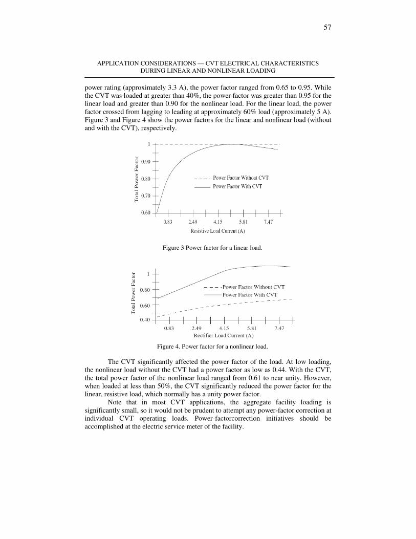
APPLICATION CONSIDERATIONS — CVT ELECTRICAL CHARACTERISTICS

DURING LINEAR AND NONLINEAR LOADING

57

power rating (approximately 3.3 A), the power factor ranged from 0.65 to 0.95. While

the CVT was loaded at greater than 40%, the power factor was greater than 0.95 for the

linear load and greater than 0.90 for the nonlinear load. For the linear load, the power

factor crossed from lagging to leading at approximately 60% load (approximately 5 A).

Figure 3 and Figure 4 show the power factors for the linear and nonlinear load (without

and with the CVT), respectively.

Figure 3 Power factor for a linear load.

Figure 4. Power factor for a nonlinear load.

The CVT significantly affected the power factor of the load. At low loading,

the nonlinear load without the CVT had a power factor as low as 0.44. With the CVT,

the total power factor of the nonlinear load ranged from 0.61 to near unity. However,

when loaded at less than 50%, the CVT significantly reduced the power factor for the

linear, resistive load, which normally has a unity power factor.

Note that in most CVT applications, the aggregate facility loading is

significantly small, so it would not be prudent to attempt any power-factor correction at

individual CVT operating loads. Power-factorcorrection initiatives should be

accomplished at the electric service meter of the facility.

CIUCUR, V., V.

58

3. APPLICATION CONSIDERATIONS — USING THREE-PHASE INPUT

One of the drawbacks of using a CVT is its inability to protect equipment from

voltage interruptions. A traditional CVT can protect equipment down to approximately

40% of nominal voltage. A company in the midwestern U.S. has introduced a

prototype CVT that protects equipment from deep voltage sags and brief power

interruptions.

Figure 5 Schematic of a ride-through transformer.

As shown in Figure 5, the ride-through transformer (RTT) is designed to

protect single-phase process controls. Unlike traditional CVTs, the RTT uses all three

phases of supply voltage as its input. This enables the RTT to access energy in

unsagged phases of the supply voltage during one- or two-phase voltage sags and

interruptions.

EPRI PEAC tested the prototype, 1-kV, 480-V RTT [12] to determine its

ability to protect process controls during single-phase, two-phase, and three-phase

voltage sags and interruptions. The particular prototype acquired for testing was

connected to a load bank that consisted of a mixture of 12 industrial control

components: ice-cube relays, motor starters, contactors, a programmable logic

controller, a linear dc power supply, and a switch-mode power supply. Figure 6 a and

Figure 6 b show the response of an RTT to phase-to-neutral and phase-to-phase sags.

APPLICATION CONSIDERATIONS — CVT ELECTRICAL CHARACTERISTICS

DURING LINEAR AND NONLINEAR LOADING

59

Figure 6. Performance of a ride-through transformer (RTT) during a ten-cycle voltage

interruption and voltage sag. Voltage regulation of an RTT during a single-phase voltage

interruption (top: input; bottom: output).

To get the most out of a CVT with a three-phase input, the most trouble-free

voltage phases of the electric-service supply will have to be determined. For example,

if most voltage sags occur on phase A or B, then the center tap on the transformer

primary should be connected to phase C. Although this prototype transformer promises

to retail at a price substantially higher than the price of a traditional, single-phase CVT,

the price differential can be greatly reduced by a reduction in size. Because the

performance of a traditional CVT greatly depends upon loading, CVTs are often

oversized for the connected load. A smaller but more loaded RTT should be able to

perform as well as the derated, traditional CVT.

CIUCUR, V., V.

60

4.CONCLUSIONS The test results revealed that the prototype RTT protected the connected

process controls from most of the applied voltage sags and interruptions. Besides, it

was observed that RTT performance greatly depended on the phase configuration (that

is, single-, two-, or three-phase) of the voltage sags or interruption and, to a much

lesser extent, on the loading of the RTT output. It was observed that the RTT

performed like a typical CVT during three-phase voltage sags

REFERENCES

[1]. Sola/Hevi-Duty Corp., About Sola/Hevi-Duty, www.sola-hevi-

duty.com/about/solahist.html, October 18, 2002.

[2]. Advance Galatrek, CVT Background Data, http://www.aelgroup.co.uk/hb/hb003.htm,

October 18, 2002.

[3]. EPRI, System Compatibility Projects to Characterize Electronic Equipment Performance

under Varying Electric Service Supply Conditions, EPRI PEAC, Knoxville, TN, May 1993.

[4]. Godfrey,.,Ferroresonance, http://www.physics.carleton.ca/courses/75.364/mp1html/node7.html October 18, 2002.

[5]. Cadicorp, Ferro-Resonance, Technical Bulletin 004a, www.cadicorp.com, October 18,

2002.

[6]. Groupe Schneider, Ferroresonance, No. 190, www.schneiderelectric.com, October 19,

2002.

[7]. IEEE, Standard for Ferroresonant Voltage Regulators, IEEE Std. 449-1998, Institute of

Electrical and Electronics Engineers, Piscataway, NJ, 1998.

[8]. EPRI, Sizing Constant-Voltage Transformers to Maximize Voltage Regulation for Process

Control Devices, PQTN Application No. 10, EPRI PEAC, Knoxville, TN, October 1997.

[9]. EPRI, Ferro-Resonant Transformer Output Performance under Varying Supply

Conditions, PQTN Brief No. 13, EPRI PEAC, Knoxville, TN, May 1993.

[10] EPRI, Ferro-Resonant Transformer Output Performance under Dynamic Supply

Conditions, PQTN Brief No. 14, EPRI PEAC, Knoxville, TN, January 1994.

[11] EPRI, Ferro-Resonant Transformer Input Electrical Characteristics during Linear and

Nonlinear Loading, PQTN Brief No. 16, EPRI PEAC, Knoxville, TN, February 1994.

[12] EPRI, Testing a Prototype Ferro-Resonant Transformer, EPRI PEAC, Knoxville, TN,

unpublished.


EMBEDDED DEVLOPMENT ENVIROMENT TO CONTROL

THE CIM-SYSTEMS

ANGELA EGRI1, ADRIAN TUL BURE

2 , VALI SARB3

Abstaract :In this papers is presented the Embedded Development Environment kit EVA167

This contain the software tools and the hardware device for real-time evaluation of the C167

microcontroller. The board is delivered with two static RAMs which con be extended until 2

Mbytes. With the help of open drain circuit on Port7 one can achieve the combination of more

PWM outputs through different pull up configuration/connections . This provides the short

circuit for any PWM channel.

Key words: Embedded Development Environment, PWM, kit EVA167 and CMOS

microcontroller.

1. SOFTWARE PRESENTATION

A classical Program Development Environment (DE) is used to develop

applications for systems with only one target and host system. Thereby is possible to

run a application directly from the Integrated DE.

In an Embedded Development Environment (EDE) this is no longer true. To

run an application for a embedded system, a simulator or target hardware is required.

The EDE can both compile error free a module and offers a number of simulators and

target hardware.

The used Embedded Development Environment EDE can be divided into three

main parts:EDIT, BUILD and DEBUG, like in the fig.1 In the Edit part one can select

the toolchain, create and maintain a project, edit some sources to be used in a project

and specify the development options. In the Build part a makefile (created by the Edit

1 PhD Assoc. prof at Eng, University of Perosani

2 PhD Lecturer. Eng at University “1 Decembrie 1918” of Alba Iulia

3 PhD Lecturer. Eng at University of Perosani

EGRI,A., TULBURE, A., SARB, V.

62

part) is used to invoke the needed toolchain components, resulting in an absolute object

file. In the Debug part one can use this absolute file to debug proposed project.

Figure 1. Development flow of the EDE

The Evaluation Board offers two possibilities for connection to a PC:through

serial ports COM1 or COM2 and the asynchronous or synchronous device of the

SAB80C167. The serial ports of the PC can be set in the configuration file.

In order to comunicate with the PC the evaluation board EVA167 uses the

programm which contains the following files /2/, /3/:

- MON16X.EXE (monitor user interface), - MON16X.OVL (overlay file)

- BOOT.167 (bootloader file), - MON.167 (loadable monitor)

- MON16X.CFG (configuration file), - MON16X.SCR (start recorder file)

- LD167.BAT (loader for microcontroller programs),

- TERM.OUT (demo to the TERM command),

- TEST.REC (demo recorder file)

The monitor program MON16X uses a memory region, which will be

downloaded into the board memory. MON16X have available several command

groups, like as: memory, register, execute, monitor and other commands.

The attached batch file LD167.BAT is able to load files directly. It recognizes

automatically the following formats: Tasking-format (*.out), OMF166-format (*.66),

and HEX-format (*.H66). By starting the monitor, this searches first for the

configration file „MON167.CFG“. This file contains parameters, which the monitor

users to configure the experimental board.

The following file „TERM C“ shows a clasical program, that wants to use the

computer as a terminal /2/.

Toolchain sel.

Tools option

Editor

Management

Make

Compiler

Assembler

Linker

Locator

Debbuger

Simulator

EDIT BUILD DEBUG

EDE

Makefile Abs.file

EMBEDDED DEVLOPMENT ENVIROMENT TO CONTROL THE CIM-SYSTEMS

63

/***************************************************************************/

/* TERM.C Program demonstrativ pentru MON167 */

/* */

/***************************************************************************/

#include <c166.h> /* Declararea bibliotecilor necesare */

#include <reg167.h>

#define MAIN_C

/* Parametrii biţilor */

#define BIT15 0x8000

#define BIT14 0x4000

...

/* Definirea perioadelor PWM (în unităţi timer i.e. 400ns / bit) */

#define PROC_FREQ 20000000L /* Frecvenţă CPU (în Hz) */

#define PWM_FREQ 1000L /* Frecvenţă Timebase (în Hz) */

#define GPT1_FREQ (PROC_FREQ / 8L) /* Frecvenţă de clock GPT1 */

...

#define PWM_PERIOD (GPT1_FREQ / PWM_FREQ) /* Perioada PWM (unităţi GPT1 ) */

#define DUTY_CYCLE 90L /* % PWM Duty Cycle */

#define HIGH_PERIOD ((PWM_PERIOD * DUTY_CYCLE) / 100L)

#define LOW_PERIOD (PWM_PERIOD - HIGH_PERIOD

2. HARDWARE DESCRIPTION

The used controller is a derivative of the C16x Family of full featured single-

chip CMOS microcontrollers /1/, /2/. It combines high CPU performance with

peripheral functionality and enhanced IO-capabilities, like in fig.2.

A lot of features contributes to his performance: short execution time per

instruction acceptance of many data types like bit, byte and word, internal on-chip

integrated RAM-Memory, interrupt vectors with more Priority Levels, Peripheral

Event Controller and Intelligent Peripheral Components.

Port P0 (fig.1. SAB80C167 right) consists of the two 8-bit bidirectional I/O

ports. Both are bit-wise programmable via direction bits as input or output. For a input

configuration, the output driver is put into high-impedance state.

Port P1 consists also of the two 8-bit bidirectional I/O ports. This port is used

as the 16-bit address bus (A) in demultiplexed bus modes and also after switching from

a demultiplexed bus mode to a multiplexed bus mode.


64

Table 1

Connection pins of the Port 7

Figure 2. Block-diagram of the

microcontroller

Port P2 (fig.2. ) is a 16-bit bidirectional I/O port. It is also bit-wise

programmable for input or output via direction bits. Port 2 outputs can be configured as

push/ pull or open drain drivers. The input threshold of Port 2 is selectable (TTL or

special).

Port P3 is a 15-bit (P3.14 is missing) bidirectional I/O port also bit-wise

programmable. The input threshold of Port 3 is selectable (TTL or special). The

Port 3 pins can serve for alternate functions like Timers, Transmisions Units,

Ext. memory signals and system clock.

Port P4 is an 8-bit bidirectional I/O port. It is bit-wiseprogrammable. In case of

an external bus configuration, Port 4 can be used to output the segment address lines.

Port P5 is a 16-bit input-only port with Schmitt-Trigger Properties. The pins of

Port 5 also serve as the (up to 16) analog input channels for the A/D converter, where

P5.x equals ANx (Analog input channel x), or they serve as timer inputs:

Port P6 is an 8-bit bidirectional I/O port. Port 6 outputs can be configured as

push/ pull or open drain drivers. The Port 6 pins also serve for alternate functions like:

chip select, master hold, bus request.

Port P7 is an 8-bit bidirectional I/O port. It is bit-wisePort 7 outputs can be

configured as push/ pull or open drain drivers. The input threshold of Port 7 is

selectable (TTL or special). The following Port 7 pins also serve for alternate functions

like: pwm- and CapCom-Output.

Port P8 is an 8-bit bidirectional I/O port. The input threshold of Port 8 is

selectable (TTL or special). Many Port 8 pins also serve for alternate functions like

CapCom Outputs.

The on chip PWM unit can operate in four differentmodes /3/, /4/: I) PWM

standard mode 0 (EdgeAligned PWM); II) PWM symmetric mode 1 III) Burst mode

and IV) Single shot mode. Generally the output signal is set on “logic 1” when the

counting value is greater or equal than register from PWx.

P7.0 POUT0, PWM model ch 0 out

P P7.1 POUT1, PWM model ch 1 out

O P7.2 POUT2, PWM model ch 2 out

R P7.3 POUT3, PWM model ch3 out

T P7.4 CC28IO, In /compare out ch 28

P7.5 CC29IO, In /compare out ch 29

7 P7.6 CC30IO, In /compare out ch

30

P7.7 CC31IO, In /compare out ch

31


65

3. MEASUREMENTS AND CONCLUSIONS

The kit EVA167 contain the software tools and the hardware device for real-

time evaluation of the C167 microcontroller. The board is delivered with two static

RAMs which con be extended until 2 Mbytes. With the help of open drain circuit on

Port7 one can achieve the combination of more PWM outputs through different pull up

configuration/connections [4], [5]. This provides the short circuit for any PWM

channel.

Fig. 3, 4 and 5 shows the measurement results by scope at port 7 for different

sets of the control registers.

Figure 3. PWM-signal from microcontroller.

Measurement by 2 kHz and duty cycle 90%.






66

The measured signals are used to control the CIM-System of figure 5. The

results of ghrafical simulation was presented in figures 7,8,9,10.

This control task needs semnale rapide and high resolution signals. The

achieved results demonstrated the flexibility of the programmable logic compared with

the wiring logic. By setting some program-variables the parameters of the generated

signals can be adjusted without modifying the hardware part.

Figure 6. CIM-System

Figure 7. Position Figure 8. Voltage

Figure 9. Curent Figure 10.Velocity


67

REFERENCES

[1] Siemens C167 Derivatives, 16 Bit Microcontrollers, User Manual 1996

[2] Ertec GmbH, Evaluation Board EVA167, Erlangen 1993

[3] Mattheis/Storadt, MC-Tools 17, Otmar Feger, Hard+SoftwareVerlag,

Traunstein 1999

[4] A.Tulbure, M.Erdmann, 16 Bit Embedded System to Control the High Power

Supply Units, SIMPRO 2005, Petrosani 2005

[5] A..Tulbure, A..Egri, R..Joldes, Cages Switching at an induction machine using

the 16-bit microcontrolle, MicroCAD, University of Miskolc 2007.


A SHORT PRESENTATION OF THE DYE SENSITIZED NANOSTRUCTURES SOLAR CELLS

LARISA MĂGHERUŞAN1

Abstract: The dye sensitized solar cells (DSSC) belong to a group of thin layer cells where the

absorption process occurs inside the dye molecules adsorbed on a very porous transparent

surface of TiO2 nanoparticles. Under illumination the cell gives rise to a voltage between the

two electrodes and also to an electric current through an external load.

Keywords: nanoparticles. solar cells, photoelectrochemical

1. INTRODUCTION

Historically speaking the 19th century states the beginning of the dye-

sensitization procedure along with the invention of photography. The first meaningful

study of dye-sensitization of semiconductors was represented by the work of Vogel in

Berlin back in 1873. In his research silver halide emulsions were sensitized by dyes to

produce black and white photographic films.

In the early 1990’s in the Laboratory of Photonics and Interfaces Switzerland,

professor Grätzel and his co-workers used a combination of nanostructured electrodes

and some effective charge injecting dyes and managed to develop an efficient energy

conversion solar cell (7% in 1991 and 10% in 1993). His device was called the dye-

sensitized nanostructured solar cell or the Grätzel cell in his honour.

What makes these cells apart from the conventional ones is the fact that they

are photoelectrochemical solar cells, meaning that they use a liquid electrolyte or other

ion-conducting phase as a charge transport medium, which seems to lead to high

efficiencies and good long-term stability. As a result, many research groups took a

great interest in studying this kind of cells, especially in terms of finding new materials

that could improve the manufacture aspects and costs.

1 PhD. Student Physician

A SHORT PRESENTATION OF THE DYE SENSITIZED

NANOSTRUCTURES SOLAR CELLS

69

Before explaining the basic operating principle of the dye-sensitized

nanostructured cell, I need to remind that the process of converting light into electric

current in an organic photovoltaic cell is performed in four stages:

1. Light absorption followed by the formation of excitons;

2. Exciton diffusion towards an electric field region;

3. Charge separation in the electric field region;

4. Charge transport towards electrodes in order to give rise to a direct current

passing through a consumer load.

The dye sensitized solar cells (DSSC) belong to a group of thin layer cells

where the absorption process occurs inside the dye molecules adsorbed on a very

porous transparent surface of TiO2 nanoparticles. The dye excitation is followed by the

electron injection in TiO2 and the dye regeneration by the use of a reduction-oxidation

couple such as I-/I3

-. The porous nanocrystalline TiO2 electrode structure has a specific

role to increase the internal surface area of the electrode in order to allow a large

enough amount of dye to be contacted both by the TiO2 electrode and the electrolyte.

The injected electrons are then transported to the front contact electrode (a transparent

conducting oxide)..

Figure 1 Nanostructured titan dioxide material.

The size of the particles is about 20 nm

2. OPERATING PRINCIPLE

In its simpliest configuration, the DSSC cell consists of a transparent

conducting electrode covered by porous nanocrystalline titan dioxide (nc-TiO2), dye

molecules attached to TiO2 surface, an electrolyte containing a reduction-oxidation

couple such as (I-/I3

-) and a catalyst coated counter-electrode.

Under illumination the cell gives rise to a voltage between the two electrodes

and also to an electric current through an external load.

The TiO2 electrode has a thickness of 10 m, with an average size of the

particles and also of the pores of about 20 nm. Its internal surface area is thousand

times larger than the geometrical surface of the electrode. The most important thing

regarding the titan oxide is the fact that it is a semiconducting material having an

enough large band gap in order to absorb radiation only below 400 nm. In this way the

dye molecules may absorb most of the radiation from the solar spectrum.

MĂGHERUŞAN, L.

70

Figure 2

A schematic representation of the DSSC structure

A SHORT PRESENTATION OF THE DYE SENSITIZED

NANOSTRUCTURES SOLAR CELLS

71

The incident photon is absorbed by the dye molecule attached to the

nanocrystalline TiO2 material. An electron initially in an S0 fundamental molecular

state is transferred to a energetically higher S* state. The excited electron is then

injected in the conduction band of the TiO2 particle leaving the dye molecule into an

oxidized S+ state. The injected electron percolates through the porous nanocrystalline

structure towards the transparent conducting electrode (anode) and eventually passes

through the external consumer to the counter-electrode (cathode). Here the electron

goes to the triiodide from the electrolyte and facilitates the formation of iodine. The

cycle is completed by the reduction of the oxidized dye from the electrolyte.

The chemical reactions taking place during a working cycle are as follows:

At the Anode: *0 ShS →+ ν light absorption

)(* 2TiOeSS−+ +→ electron injection

−−+ +→+ 30232 ISIS dye regeneration

At the Cahtode: ( ) −−− →+ IPteI 323 iodine formation

For the Cell: ( ) ( )2TiOehPte−− →+ ν electron transfer from anode

to cathode

As one can observe, the working process of this cell is regenerative, no

substances being either consumed or produced during the cycle.

Figure 3 Working principle of the DSSC configuration

MĂGHERUŞAN, L.

72

The electrodes of a standard DSSC structure are transparent conducting oxide

coated glass substrates, between which the cell is assembled. The conducting coating

of the substrate works as a current collector while the substrate material is as a support

structure to the cell and also a sealing layer between the cell and the external

environment. Fluorine-doped tin oxide (SnO2:F) and indium tin oxide (In2O3:Sn or

ITO) are the most frequently materials used as transparent conducting oxides in thin

film photovoltaic cells. The dyes most used for sensitization in these cells are the

metalo-organic ruthenium complexes and for the counter-electrode the most suitable

material seems to be the platinum used as a catalyst coat for the transparent conducting

oxide substrate.

3. SOME SPECIFIC CHARACTERISTICS OF THE DSSC CONFIGURATIONS

Unlike a pn semiconductor jonction solar cell, in a DSSC structure the light

absorption and the carrier transport are taking place in separate materials. Much more,

the charge separation involves different kinetic and energetic mechanisms at the dye-

semiconductor-electrolyte interfaces. Because of its porous structure the electrode acts

like a network of individual particles through which electrons percolate by hopping

from one particle to the next. The small size of the particles does not allow the

formation of a space charge region and consequently there will be no built-in electric

field to drift the charge carriers. transport and therefore the transport of electrons

cannot be drift in an electric field.

And finally, but not less important, in DSSCs the opposite sign carriers travel

through different regions and so the recombination processes may be significant only at

interfaces. This way the necessity of a pure semiconductor is not so acute.

The highest efficiencies for these cells (Green 2001, Grätzel 2000,

Nazeeruddin et al. 1993, O'Regan & Grätzel 1991) were obtained in Switzerland by the

Grätzel group who has reported a top efficiency of 110.5% in 1996.

REFERENCES

[1]. Halme, J., Dye-sensitized nanostructured and organic photovoltaic cells: technical review

and preliminary tests, Helsinki University of Technology, 2002;

[2]. Brabec, C.J., V. Dyakonov, J. Parisi, and Sariciftci, N.S., Organic Photovoltaics:

Concepts and Realization; Vol. 60, Berlin, 2003;

[3]. Hoppe H, Sariciftci, N.S., Organic Solar Cells: An Overview, Linz Institute for Organic

Solar Cells, Austria, 2004.


USING THERMOCOUPLES IN PROGRAMMABLE SYSTEMS FOR MEASURING TEMPERATURE

NICOLAE PĂTRĂŞCOIU1 ADRIAN TOMUŞ2 CECILIA ROŞULESCU3

Abstract: Thermocouples are the most popular temperature sensors. They are cheap,

interchangeable, have standard connectors and can measure a wide range of temperatures. The

main limitation is accuracy, system errors of less than 1°C can be difficult to achieve with usual

system measurement. Using a data acquisition system it can be possible to reduce measurement

system errors. We propose a temperature system measurement and virtual instrument based on

NI USB 6008 data acquisition module.

Keywords: thermocouple, data acquisition, USB-6008, virtual instrument

1. THERMOCOUPLE

Thermocouple is temperature sensor suitable for use with any make of

instrument designed or programmed for use with the same type of thermocouple.

Thermocouple is based on the principle that when two dissimilar metals are joined a

predictable voltage will be generated that relates to the difference in temperature

between the measuring junction and the reference junction.

Starting from this observation is obvious that to measure the relative

temperature Tx is needed to establish a reference and this is the temperature

corresponding freezing point (“ice-point” temperature) of water, Tice. That means a new

junction is added and held in an ice bath at Tice (0°C/32°F). The thermocouple circuit

shown in Fig. 1 represents the basis upon which thermocouple standard tables have

been established. The standards community together with modern metallurgy has

developed special material pairs specifically for use as thermocouples.

Table 1 displays industries eight popular standard thermocouples and their

typical attributes. Manufacturers may fabricate thermocouples of a given type with

variations in composition; however, the resultant temperature versus voltage

1 Assoc.Prof.Eng.Ph.D., University of Petroşani

2 Assist.Drd.Eng., University of Petroşani

3 Prof. “Grigore Geamănu” School

PĂTRĂŞCOIU, N., TOMUŞ, A., ROŞULESCU, C.

74

relationships must conform to the thermoelectric voltage standards associated with the

particular thermocouple type.

Standard mathematical power series models have been developed for each type

of thermocouple. These

power series models use

unique sets of coefficients

which are different for

different temperature

segments within a given

thermocouple type. Unless

otherwise indicated, all

standard thermocouple

models and tables are

referenced to zero degrees

Centigrade, 0°C.

Equation (1) illustrates the power series model used for all thermocouples except

K type, which is illustrated by equation (2) where the exponential term is added to

account for special effects.

These equations together with the coefficients Ci and Ai have been adopted as

standards by the American Society for Testing and Materials (ASTM) and the

International Electrotechnical Commission (IEC).

These equations with their different sets of coefficients are difficult to use in

directly determining actual temperatures when only a measured thermocouple voltage

[VTC] is known. Therefore, inverse models have been developed to determine

temperatures from measured thermocouple voltages. Equation 3 represents this inverse

model.

VTC Tc Tx

Tv

Tice

Fig.1. Thermocouple Topology

( )( ) [ ]∑=

⋅=n

i

ixi mV,TCVTC

0

(1)

( )( ) ( ) [ ]∑=

−⋅⋅+⋅=

n

i

ATAixi mV,eATCVTC x

0

2

021 (2)

( )( ) [ ]∑=

⋅=n

i

oiix C,VTCDT

0

(3)

Table 1

Type Materials Typical Range

[O

C]

T 1,2

Copper (Cu) vs Constantan -270 to 400

J 1,3

Iron (Fe) vs Constantan -210 to 1200

K Chromel vs Alumel -270 to 1370

E Chromel vs Constantan -270 to 1000

S (Pt-10%Rh) vs Pt -50 to 1768

B (Pt-13% Rh) vs (Pt-6% Rh) 0 to 1820

R (Pt-13%Rh) vs Pt -50 to 1768

N (Ni-Cr-Si) vs (Ni-Si-Mg) -270 to 1300

USING THERMOCOUPLES IN PROGRAMMABLE SYSTEMS FOR MEASURING

TEMPERATURE

75

where VTC is in millivolts.

2. TEMPERATURE ACQUISITION SYSTEM

When a replacement thermocouple is required, it is of the utmost importance that

the type of thermocouple type used in the replacement matches that of the measuring

instrument. Different thermocouple types have very different voltage output curves. It

is also required that thermocouple or thermocouple extension wire, of the proper type,

be used all the way from the sensing element to the measuring element. Large errors

can develop if this practice is not followed.

This acquisition system is based on using the module NI USB-6008 that is

controlled by an application developed in LabVIEW and called virtual instrument.

The NI USB-6008 provides connection to 8 analog input (AI) single-ended or 4

differential, software selectable channels, 2 analog output (AO) channels, 12 digital

input/output (DIO) channels, and a 32-bit counter with a full-speed USB interface. For

this application we use two differential analog inputs that range can be chosen between

± 10 V ... ± 1 V and is chosen the input range ± 1 V.

One of the inputs (AI0) is

used to retrieve the signal from the

sensor and the other input (AI1) is

used to retrieve the signal from a

thermistor used for cold junction

(CJC) temperature compensation.

Considering the field of

measurement 0 ... 200 oC the

maximum voltage generated is

obtained for the K thermocouple

and for the limit about 200 oC the

voltage is only 20.872 mV. In

these conditions to use the entire

dynamic range of the converter

that is -2.5 ... 2.5 V is necessary to

use an amplifier with a gain of 120. To achieve this gain is used an instrumentation

amplifier, such as the INA114 which gain G is given by the relation:

yields a value of required resistance RG by about 1 kΩ and is choose a variable

resistance with value of 1 kΩ so that is offered a possibility of carrying out an

adjustment of the gain. Measured thermocouple voltage (VTC) adapted to cover the

dynamic range of the analog-digital converter becomes input voltage UA0

To achieve the compensation of cold junction temperature is used a thermistor

with negative temperature coefficient (NTC) that has the following parameters: RT=10

GR

k501G

Ω+= (4)

U1

INA114AP

6

4

7

3

2

5

1

8

C1100nF

C2100nF

TO_USB6008_A0

HDR1X2

VCC

5V

VEE

-5V

RG

2kΩKey=A 5%

R1 10kΩ1%

THERMOCOUPLE

HDR1X2

Fig.2. Precision Instrumentation Amplifier


76

kΩ nominal resistance @ 25 oC, Steinhart-Hart equation parameters: A = 0.001129148;

B=0.000234125; C = 8.76741E-8.

Thermistors are widely used because of their sensitivity, small size, ruggedness

and low cost. Thermistors have an electrical resistance that varies non-linearly with

temperature. The R-T characteristics of most thermistors can be described by the

Steinhart-Hart equation:

( ) ( )[ ] 13 −⋅+⋅+= TT RlnCRlnBAT (5)

where T is the absolute temperature

(in Kelvin) and A, B, and C are

constants whose values depend on

the constructive parameters of the

thermistor and which for this

application have been presented

above.

As the NI USB-6008 module

analog input measures only

voltage, we will need to provide a

current source to convert the

resistance to voltage. For this is

used Howland mounting (fig.3)

like a constant current source. The amount of current through thermistor does not

depend on the resistance RT and it is given by the relationship:

Applied tension to the analog input AI1, UA1 is proportional to the amount

thermistor resistance, as the relationship:

wherefrom

The two tensions UA0 and UA1 are applied to the data acquisition module NI

USB-6008 at the analog inputs AI0 respectively AI1.

Fig.3. Thermistor used to CJC compensation

U1AOPA1013CN8

3

2

4

8

1

R1 10kΩ1%

R2 10kΩ1%

R3 10kΩ1%

R410kΩ1%

VCC

2.5V

RT

10kΩ1%

VDD

5V

U1

U2

TO_USB6008_A1

HDR1X2

2

3

1

1

22

3

4

4

T UR

1U

R

RU

R

R

R

1I ⋅=

⋅−⋅⋅= (6)

( ) 2T2

2

1

3

T1

1

2

2

112

3

T1A U

R

2RU

R

R1

R

1RU

R

R

R

R1UU

R

RU ⋅⋅=⋅

+⋅⋅=⋅−

+⋅−⋅= (7)

122

AT UU

RR ⋅

⋅= (8)


TEMPERATURE

77

3. VIRTUAL INSTRUMENT Virtual instrument (VI), which is the acquisition process administration, has two

major components: the diagram bloc that represents the properly program and the front

panel that represents the user interface.

The main programming structure from the diagram bloc of virtual instrument for

this application, shown in Fig. 4 is a While Loop and acquisition process is performing

by using DAQmx functions.

The first function used is the NI-DAQmx Create Virtual Channel which creates

a virtual channel corresponding to two analog inputs and adds it to a task. The second function used is the DAQmx Start Task. This function explicitly transitions a task to

the running state. In this application, in the running state, the function starts the task

which performs the specified acquisition. The third function used is the DAQmx Read

and this function reads samples from the specify task or virtual channels. In this

application, the function reads analog inputs AI0 and AI1.

The value of voltage UA0 taken by the analog input AI0 is displayed as Thermocouple Voltage and is used to determine temperature of the thermocouple. To

determine the thermocouple temperature is used relationship (3) customized for

different thermocouples and specific areas of their temperatures. To achieve voltage-temperature conversion is used a SubVI (V→T) that has like base element a Case

structure. Value wired to the Case selector terminal that select which case is executed

at a time is generated by the user via front panel control Thermocouple type. The selection of areas of measurement for each thermocouple is done by comparing the

values of these areas limits, taken from the static characteristic to the corresponding

generated voltage. Practically, in this way, it generated a number of cases equal to the

number of subdomains and these cases are properly selected.

Fig.4. Diagram bloc of the virtual instrument


78

The relationship between the temperature difference and the output voltage of a

thermocouple is nonlinear and is given by a complex polynomial equation. As mentioned above, to use relationship (3) is necessary to choose values of Di

coefficients in agreement with ITS90 standard. To achieve this requirement is used

subVI (V→T), shown in Fig. 5, whose block diagram is exemplified for a

thermocouple type K used for the temperature range 0 ... 500 ° C. For type K

thermocouple field measurement is -200 ... 1375 oC, and this area is divided into 3

subdomains such -200 ... 0 °C, 0 ... 500 °C, respectively 500 … 1375 °C, each subdomain is characterized by different coefficients for the static characteristic defined

by relationship (3). The selection of each of the three cases is based on the values of

tension UA0 generated for 0 oC and 500

oC ie 0 and respectively 20644 µV.

Virtual instrument ensure also the selection of units for measuring temperature

via control Temperature Units on the front panel by selecting the corresponding

relations for conversion. The front

panel is the user

interface of the

virtual instrument

and it is built with

controls and

indicators, which

are the interactive

input and output terminals of the

virtual instrument. The

front panel for this

application, Fig.6,

contains controls

mentioned above, plus controls for setting

parameters of the

Howland mounting i.e. Howland Resistance and

Howland Voltage. Indicators on the

front panel are used to

display the measured

temperature

(Temperature) and also

to display additional values such as voltage generated by thermocouple

(Thermocouple Voltage), the uncompensated temperature (Uncompensated TC Temperature), reference junction temperature (CJC Temperature) and the thermistor resistance value (Thermistor Resistance)

Fig.5. SubVI Voltage to Temperature (V →T)


TEMPERATURE

79

4. CONCLUSIONS

Using the data acquisition system and virtual instrument enables a severe reduction of measuring errors. This reduction is possible by choosing appropriate static

characteristic of thermocouple depending of type of thermocouple, domains and

subdomains of the temperature

Changes into measurement scheme may be further made because the user has

the possibility to select through the controls on the front panel type thermocouple used

at a time and area of use thereof.

REFERENCES

[1]. Pătrăşcoiu N. , Mândrescu C., Senzori şi traductoare. Ed.Universitas, Petroşani,

2000

[2]. Pătrăşcoiu N., Sisteme de achizitie si prelucrare a datelor. Instrumentatie virtuala

Ed. Didactica si Pedagogica, Bucuresti, 2004

[3]. Ionescu G., Traductoare pentru automatizari industriale. Ed. Tehnica, Bucuresti,

1985

[4]. Sinclair, J. Dunton. Practical Electronics Handbook. Sixth Edition. Newnes,

London, 2007

[5]. * * *, NI USB-6008/6009 User Guide and Specifications. 371303K-01, National

Instruments Corporation, Dec.2007

[6]. * * *, NI-DAQmx for USB Devices. Getting Started Guide. 324147E-01, National

Instruments Corporation, Dec.2007


VISUAL BASIC APPLICATION FOR CALCULATING THE FLOATATION FLOWSHEETS

BRANA LILIANA SAMOILĂ1, MARIUS DANIEL MARCU2,

ILIE UŢU3

Abstract: The paper deals with the simple floatation circuits’ design, which is a problem of

great importance in floatation circuit design and optimization. We achieved the algorithm,

determining the recurrent relations and establishing the restriction conditions. Using the results

of our research, we elaborated a Visual Basic Application which allows the calculation of

quantities and contents in every point of a floatation circuit, for any number of operations. It’s

an easy to use, conversational application that allows studying more variants in order to

establish the optimum one, sparing the researchers’ and designers’ time and effort.

Keywords: floatation, application, design

1. INTRODUCTION

These last years have seen significant developments in mineral processing

technologies, particularly in hydrometallurgy, bio-hydrometallurgy and mineral

liberation.

Analyzing, optimizing and designing flotation circuits using models and

simulators have improved significantly over the last 15 years.

In order to calculate a floatation technological flow sheet, we should

previously know the following elements:

- the quantities of material in the feed, output products and all intermediate

points;

- valuable mineral contents in all of the formerly mentioned products;

- water quantities, that is dilution, for each product.

It becomes necessary to calculate the flow sheet in the following situations:

- to design an installation or a new section in an installation;

1 Ph.D Associate professor,Eng at University of Petrosani



VISUAL BASIC APPLICATION FOR CALCULATING

THE FLOATATION FLOWSHEETS

81

- to know the products characteristics all along a technological circuit, for a

certain functioning regime.

From time to time, we must know the characteristics of an installation, in order

to be able to modify or to correct the existing technological scheme without

supplementary investments as well as to improve the technical and economical

indexes. That may be needed when the raw material quality has been changed or the

customers requests are different.

2. FLOATATION CIRCUITS DESIGNING VISUAL BASIC APPLICATION

Using the balance equations written for

different types of monometallic mineral simple

floatation circuits, we calculated the quantities and

valuable metal contents in each point of the circuit.

We expressed these parameters only

depending on weight recoveries for each operation

(vik, vcj), total weight recovery (v), feed quantity (A)

and contents in: feed (a), concentrate (c), floated

products of each enriching operation (dk) and

cleaning operation (gj).

From our point of view, a floatation circuit

can be represented as in figure 1, where the notation

significance is:

k - enriching operation number;

j - cleaning operation number;

(xk) - vector of enriching operation parameters;

(yj) - vector of cleaning operation parameters.

It must be said that the

operations were numbered from

the circuit end to the beginning,

in order to express the relations

in a more simple form.

Using Visual basic

programming tools, we

developed an application that

allows the calculation of any

floatation circuit.

This is a powerful

process simulation software

package, a user-friendly steady-

state simulator that allows

mineral processing engineers and

scientists to model floatation

operations with available experimental data and determine optimal configuration that

FLOATATION

CIRCUIT

A

v

(vik)

(vcj)

a

c

(dk)

(gj)

B

C

(Dk)

(Fk)

(Ej)

(b)

(fk)

(Gj)

(ej)

Fig. 1 Simple floatation

circuit diagram

Fig. 2 Main window

SAMOILĂ, B., L., MARCU, M., D., UŢU, I.

82

meets production targets. The simulator can also assist plant designers with sizing unit

operations required to achieve given circuit objectives.

The software package contains functions that can:

- manipulate experimental data,

- calculate coherent material balances, sizes and settings of unit operations,

physical properties of the processed materials,

- simulate plant operation and display results in tables.

In the main window, the operator has to introduce the values of the input

variables, including the number

of both kinds of operations

(figure 2).

The data are verified and,

if they are not properly

introduced, a message appears to

worn the operator (figure 3).

After introducing the

number of enriching operations,

a window is opening to introduce

the values of weight recoveries

and contents in the floated

outcomes (figure 4).

A library of flow sheet

diagrams is included and that

according to the specified

number of operations can be

visualized in order to see the

specific notations.

After the operator

introduces the number of cleaning

operations, another window opens

that allows him to introduce the

weight recoveries and floated

outcome contents in this kind of

operations (figure 5).

Further development of

this application let the data and

the results be saved. Thus, the

designer or the researcher can

compare different sets of values in

order to establish the optimum

configuration of the technological

line.

The calculation results are

displayed as a table (fig. 6).

Using such an application, time can be spared in the floatation technology

Fig. 3 Warning message

Fig. 4 Enriching operations window

VISUAL BASIC APPLICATION FOR CALCULATING

THE FLOATATION FLOWSHEETS

83

design and the accuracy of the results is improved.

3. CONCLUSIONS

The simulator offers

various powerful tools in

response to the increasing

demand for a multi-criterion and

global approach by plant

designers.

It can be used equally by

process engineers for floatation

circuits design or optimization,

by researchers for process

development, as well as by

academics for teaching process

engineering students.

Plans are already made to

extend the program and include

liberation data viewing and

model fitting for a complete

flotation circuit analysis package.

In addition, it is now

necessary to take into account the

environmental impact at each

stage of a mining project,

including water and power

consumption, waste treatment and

disposal.

The software will have to

incorporate these modern

developments. Indeed, its

structure allows the user to take

into account, at the same time, a

wide range of technological, economic and environmental aspects.

REFERENCES

[1]. Samoila, L. - Introducerea tehnicii de calcul in conducerea procesului de flotatie a

substantelor minerale utile. Doctoral thesis, Petrosani University, 1999.

[2]. Samoila, L. - Sistemul tehnologic multivariabil de flotaţie. Traductoare, modelare,

simulare.. Universitas Publishung House, 2001, 189 pp.

[3]. Harris, M.C., Runge, K.C., Whiten, W.J., Morrison, R.D. - Jksimfloat as a Practical

Tool for Flotation Process Design and Optimisation. Proceedings of the SME Mineral

Processing Plant Design, Practice and Control Conference, SME, Vancouver, 2002, pp. 461-

478.

Fig. 5 Window for cleaning operations

Window

Fig. 6 Calculation results window


SOLAR - HYDROGEN ENERGY

CAMELIA STANOI

1, ALEXANDRU LAUTARU

2

Abstract: Paper presents the damages caused by fossil fuels as well as the climate change due

to greenhouse gases, and shows that solar hydrogen energy system is a clean energy alternative

to the present polluting resources.

Key-words: fossil fuels, hydrogen, hydrides, fuel cell, electrolyzers, greenhouse gas,

renewable, power plant.

I. INTRODUCTION

Why renewable energy instead of fossil fuels?

The United Nations Climate Report 2006 shows that the global temperature of

the atmosphere will be rising up to 9 K by 2100, melting polar ice and increasing the

sea level. An average global warming of 2°C, threatens millions of people with an

increased risk of hunger and malaria.

Since the 1970’s scientists started to realize that the massive increase of CO2 in

the atmosphere emitted by cars and factories started to harm our environment. Another

gas caused by the combustion of fossil fuels, in the presence of air, is NOx. Unlike

CO2, NOx turns into acid inside our lungs when we inhale it. This acid will destroy the lung’s structure and the lungs will loose their capacity to absorb Oxygen from the air.

The molecular structure of gasoline is made up of Hydrogen (H) and Carbon

(C) molecules. When burning gasoline in an internal combustion engine, only the

Hydrogen is used for the combustion. The Carbon mixes with the Oxygen after the

combustion to form one of the most common gases: CO2, also known as the

greenhouse gas.

Coal and Oil also contain Sulphur. If we burn Oil and Coal we are generating sulphur at the same time. This Sulphur is emitted in the form of Sulphur Dioxide

1 Ph.D. Phisician at I.G. Duca School

2 Professor at I.G. Duca School


85

(SO2). SO2 also causes respiratory problems in humans. When this gas gets into the

atmosphere it combines with the water on the clouds to form sulphuric acid. Coal is the

worse fossil-fuel source of all, due to the release of Sulphur in large quantities along

with CO2, after burning. The radiation is absorbed by the CO2, as a result the

atmosphere heats up, thus warming the planet. But the worse of all is that fossil fuels

are not forever.

For reducing those consequences it will be necessary, a strong increase in the

use of renewable, non-polluting sources. The faster the costs of renewable energy are

reduced, the better we can fight global warming. The global market for renewable energy is growing dramatically.

Within the next decade many of the existing power plants in the OECD

countries will come to the end of their technical lifetime and will need to be replaced.

By contrast, the reserves of renewable energy that are technically accessible

globally, are large enough to provide about six times more energy than the world

currently consumes, forever.

The available primary sources, such as sun radiation, wind and hydro, are characterised by unfavourable characteristics, as time variability and low conversion

power density.

The recent development of wind turbines and power electronics make possible

the harvest of the solar energy and the wind energy, with acceptable costs.

We must include a much larger share of indigenous, renewable resources, so

we can develop our economies on the basis of known and predictable cost of

electricity. “Research is vital for the development of new, cheaper and more efficient

technologies.” Says Oliver Schäfer, Policy Director of EREC. “We therefore welcome

the respective European Wind, Solar, Bioenergy and smart grids Initiatives aimed at

mobilizing the critical mass of activities and actors in the renewable energy sector.” There are money for renewables but there is a total absence of policy to encourage

major investment in renewable energy.

President Bush said at Washington International Renewable Energy

Conference 2008: ".Let me start, first, by telling you that America has got to

change its habits. We've got to get off oil. Dependency on oil presents a real

challenge to our economy. As economies grow -- and we want all our economies to grow; we want people to be prosperous, we want people who are living in poverty to be able to grow out of poverty. We want there to be general prosperity, but as

economies grow, until we change our habits, there is going to be more dependency on oil."

2. HYDROGEN ENERGY SYSTEM

We need Hydrogen! Hydrogen could be adopted as a storage and transportation media. Hydrogen is

one of the most promising energy carriers that can be an alternative to fossil fuels.

Even not being available in the nature, as an elemental gas, hydrogen can be obtained

from water, alcohols, ammonia, and hydrocarbons.

STANOI, C., LAUTARU, A.

86

Therefore, is important to develope the combination of wind parks and

hydrogen production, via electrolysis. Results would be an increased hydrogen

production, for being used as fuel for combustion engines and fuel cells. Some experts

think that hydrogen will form the basic energy infrastructure that will power future

societies, replacing natural gas, oil, coal, and electricity infrastructures.

However, the electrolysis is the only mature technology that would allow

converting the harvest of renewable electricity into a fuel, able to be used, not only for

electricity reconvertion, but also in the highly demanding transport market. Water

electrolysis, as an industrial procedure, was done by the first time, in Rjucan, Norway, in 1929.

The most extended electrolysis technology is that of the bypolar, alkaline units,

using an aqueous solution of KOH. The average efficiency, of the currently available

electrolysers, is between 65 % and 70 %.

It is better known that two-thirds of the operation costs of the electrolyzers are

electricity costs. Numerous companies and researchers, in the last few years, try the

cost cutting by increasing efficiency of the process. The current offer of industrial-scaled electrolysers is low. For this reason,

prices are high, and delivery times may, often, be quite long.

Another technology, as the PEM (Proton Exchange Membrane) electrolysis,

could reach even better efficiencies, but do not seem to be effectively ready to attain

the commercial market.

Hydrogen is storable in four ways: as compressed gas, as liquid, in form of

metal hydrides, and in chemical compounds. Due to its low density, it is not effectiv to store the hydrogen gas at low pressures.

Liquified hydrogen with a temperature of –253 °C is kept in ultra-insulated

vessels at atmospheric pressure. In that case the efficiency is about 0.65 / 0.70.

Very interesting is the storage of hydrogen inside of metals, chemically bonded

as metal hydrides. The main advantage of this method is its very high energy density,

the disadvantage is the weight of the storage vessel.

Four different kinds of fuell cells, as well as combustion engines (or turbines)

and generator sets, can convert the chemical energy of the hydrogen into electricity.

In 1954, Pearson, Chapman and Fuller of the Bell Laboratory, made the

discovery that the sun can produce electricity, when its light is passed through two

different pieces of silicon, joined together like the layers of a sandwich. However, new

advances in photovoltaic cells have made the task of producing electricity from solar

power, less expensive, but it is still not practical, due to the amount of terrain it will needed for a solar farm to generate electricity.

The solar energy converted into electricity by this system must be stored and

then transferred to population centers in order to be useful. The solar-generated

electricity is used to split water into hydrogen and oxygen, using an electrolyzer. This

hydrogen could then be pumped through pipes at high pressure. When it gets to

population centers it can be used directly as fuel or be put through a fuel cell, that will

convert the hydrogen back into electricity. Fuel cell power plants also have longer life expectancies and lower costs than

their alternatives


87

Most individual fuel cells are small in size and produce between 0.5 and 0.9

volts of electricity. Therefore, any practical power plants must have a large number of

individual fuel cells. This modular nature of fuel cells is one of their biggest

advantages.

This eliminates the problems associated with large conventional power plants

which can take up to ten years to build and have a fixed capacity. Small local power

plants in urban areas have a market for their waste heat, and Japan, the U.S.A and

Canada have all tested demonstration fuel cell power plants attached to electrical grids

Fuel cells in vehicles can operate with efficiencies of 40-80% compared with 25-35% for "state-of-the-art" spark ignition engines. Ballard Power Systems, a

Canadian company which has pioneered the development of a solid plastic electrolyte

fuel cell, is installing a 100 kW demonstration fuel cell on a bus in Vancouver.

In this scenario photovoltaic cells would convert sunlight into electricity. This

electricity would be used to split water (electrolysis) into hydrogen and oxygen, in

order to store the sun's energy as hydrogen fuel.

This energy scheme is called the solar-hydrogen energy system, and its benefit is that the excess of electricity obtained through solar light is not wasted or loss

because it is used to electrolize water to obtained hydrogen, which will then be stored

and used later to produce electricity again (fig.1).

Figure 1. Solar Hydrogen Production

Another benefit, and perhaps the most important of all, is that solar and

hydrogen energy do not pollute. Since our sun will still shine, solar energy is practically everlasting. Thus solar-hydrogen energy is a clean and renewable system.

STANOI, C., LAUTARU, A.

88

For the well being of our health and environment we need to convert to Solar-

Hydrogen Energy

Hydrogen has a unique property, and that is of flameless burning, also called

catalytic combustion. By taking advantage of this property wall units for space heating

have already been designed. In this units air enters the system through the surface of a

catalytic plate made of porous ceramic with traces of platinum. Hydrogen is taken in

through the back of the plate and flameless combustion takes place inside producing

heat for the room.

Estimated hydrogen use in next 70 years according to Sigfusson Stanford (2003) shows that the hydrogen production will reach 80000 tone around 2060 (fig. 2).

But technical developments during the next few years could considerably influence the

graph.

Estimated hydrogen energy use

00.5

11.5

22.5

33.5

44.5

5

1990 2000 2010 2020 2030 2040 2050 2060 2070

En

erg

y(T

Wh

)

Fig. 2 Estimated hydrogen energy use

Hydrogen offers a way to store and regenerate electricity, does not produce

carbon dioxide, is clean, can power a vehicle or a house.

Hydrogen is a form of energy which can be stored for later use. The simplest element on the periodic table, hydrogen, is colorless, odorless, and tasteless. It's the

most common element in the galaxy, but frustratingly difficult to make on Earth.

REFERENCES

[1]. Atkins, P. W., Tratat de chimie fizică, Editura Tehnică, 1996 ;

[2]. Angerstein-Kozlowska, H., Sharp., W.A.B., Conway, E.B., in : M.W. Breiter(ed.) ”Proc.

Of Symposium on Electrocatalysis”, Electrochem. Soc., Princeton, pag.94, 1974;


89

[3]. Avramescu, A., Cartianu, P., Energetica mondiala. In perspectiva sfarsitului de mileniu, Ed.

Academiei R.S.R., Bucuresti, 1985;

[4]. Bockris, J., O’M, Srinivasan, S., “Fuel Cells. Their Electrochemistry”, McGraw Hill, New

York, 1969;

[5]. Despre politica de energie a Uniunii Europene, 2003;

[6]. Energy conversion and management, Nr. 47, pag. 46-59, 2006.

[7]. Geiger, S., Automotive Hydrogen Infrastructure – On the way to a Hydrogen Economy,

Fuel Cell Today, February 2003;

[8]. HyNor, The Norwegian Hydrogen Corridor, 2006

[9]. J.Lehmann,O.&T.Luschtinetz, C. Sponholz, A. Miege, F. Gamallo, Wind - Hydrogen

systems, 2007

[10]. CristhianJ.,Quintanilla-Aurich, Solar-hydrogen energy system, 2005;


REACTORS

ZBURLEA ELENA1

Abstract: Reactors, like capacitors, are basic to and an integral part of both

distribution and transmission power systems. Depending on their function, reactors are

connected either in shunt or in series with the network. Reactors are connected either

singularly (current-limiting reactors, shunt reactors) or in conjunction with other basic

components such as power capacitors (shunt-capacitor-switching reactors, capacitor-

discharge reactors, filter reactors).

Reactors can be installed at any industrial, distribution, or transmission voltage

level and can be rated for any current duty from a few amperes to tens of thousands of

amperes and fault-current levels of up to hundreds of thousands of amperes.

Keywords: reactors, dry type, oil immersed, air-core

1. BACKGROUND AND HISTORICAL PERSPECTIVE

Reactors can be either dry type or oil immersed. Dry-type reactors can be of

air-core or iron-core construction. In the past, dry-type air-core reactors were only

available in open-style construction (Figure 1), their windings held in place by a

mechanical clamping system and the basic insulation provided by the air space

between turns. Modern dry-type air-core reactors (Figure 2.) feature fully encapsulated

windings with the turns insulation provided by film, fiber, or enamel dielectric. Oil-

immersed reactors can be of gapped iron-core (Figure 3.) or magnetically shielded

construction.

Dry-type iron-core reactors (Figure 4) are usually used at low voltage and

indoors for applications such as harmonic filtering and power conditioning (di /dt,

smoothing, etc.).

2.APPLICATIONS OF REACTORS

2.1. General Overview Reactors have always been an integral part of power systems. The type of

technology employed for the various applications has changed over the years based on

1 Assistant., Constantza Maritime University, Depart. of Electrotechnics, Electronics

and Computer Sience, Mircea cel Batran Street, No. 104, 900663 CONSTANTA

REACTORS

91

Figure 1. Open-style reactor.

design evolution and breakthroughs in construction and materials. Dry-type air-core

reactors have traditionally been used for current-limiting applications due to their

inherent linearity of inductance vs. current.

Figure 2. Modern fully encapsulated reactor.

2.2 Current-Limiting Reactors Current-limiting reactors are now used to control short-circuit levels in

electrical power systems covering the range from large industrial power complexes to

utility distribution networks to HV (high voltage) and EHV (extra high voltage)

transmission systems.

ZBURLEA, E.

92

Current-limiting reactors (CLR) are primarily installed to reduce the short-

circuit components (especially transformers and circuit breakers) and to reduce the

short-circuit voltage drop on bus sections to levels that are consistent with insulation-

coordination practice. In summary, current-limiting reactors are installed to reduce the

magnitude of short-circuit currents in order to achieve one or more of the following

benefits:

• Reduction of electromechanical loading and thermal stresses on transformer

windings, thus extending the service life of transformers and associated equipment

• Improved stability of primary bus voltage during a fault event on a feeder

• Reduction of current-interrupting duty of feeder circuit breakers

• Reduction of line-to-line fault current to levels below those of line-to-ground

faults or vice versa

• Protection of distribution transformer and all other downstream power equipment

and devices from the propagation of initial fast-front voltage transients due to

faults and/or circuit-breaker operations

• Reduced need for downstream protection devices such as reclosers,

sectionalizers, and current-limiting fuses

• Ability to obtain complete control over the steady-state losses by meeting any

specified Q-factor for any desired frequency, a feature that is particularly important for

networks where high harmonic currents are to be damped without increasing the

fundamental-frequency loss

• Increase in system reliability

Current-limiting reactors can be installed at different points in the power

network, and as such, they are normally referred to by a name that reflects their

location/application. The most common nomenclatures are:

Figure 3. Gapped iron-core oil-immersed reactor.

• Phase reactors, installed in series with incoming or outgoing lines or feeders

• Bus-tie reactors, used to tie together two otherwise independent buses

• Duplex reactors, installed between a single source and two buses

REACTORS

93

Figure 4. Dry-type iron-core reactor (water cooled).

Figure 5. Typical phase-reactor connection.

• Neutral-grounding reactors, installed between the neutral of a transformer

and ground

2.3. Capacitor Inrush/Outrush Reactors

Capacitor switching can cause significant transients at both the switched

capacitor and remote locations.

The most common transients are:

• Overvoltage on the switched capacitor during energization

• Voltage magnification at lower-voltage capacitors

• Transformer phase-to-phase overvoltages at line termination

• Inrush current from another capacitor during back-to-back switching

• Current outrush from a capacitor into a nearby fault

• Dynamic overvoltage when switching a capacitor and transformer

simultaneously.

Capacitor inrush/outrush reactors (Figure 6) are used to reduce the severity of

ZBURLEA, E.

94

Figure 6. Typical capacitor inrush/outrush reactor connection.

some of the transients listed above in order to minimize dielectric stresses on breakers,

capacitors, transformers, surge arresters, and associated station electrical equipment.

2.4. Discharge-Current-Limiting Reactors

High-voltage series-capacitor banks are utilized in transmission systems to

improve stability operating limits. Series-capacitor banks can be supplied with a

number of discrete steps, insertion or bypass being achieved using a switching device.

For contingencies, a bypass gap is also provided for fast bypass of the

capacitors. In both cases, bypass switch closed or bypass gap activated, a discharge of

the capacitor occurs, and the energy associated with the discharge must be limited by a

damping circuit. A discharge-current limiting reactor is an integral part of this damping

circuit.

Figure 7. Typical discharge-current-limiting reactor connection.

Therefore, the discharge-current-limiting reactor must be designed to

withstand the high-frequency discharge current superimposed on the system power-

frequency current. The damping characteristic of this reactor is a critical parameter of

the discharge circuit. Sufficient damping can be provided as an integral component of

the reactor design (de-Q’ing), or it can be supplied as a separate element (resistor). See

Figure 7.

REACTORS

95

Figure 8. Typical high-voltage power-flow-control reactor connections.

2.5. Power-Flow-Control Reactors A more recent application of series reactors in transmission systems is that of

power-flow control

(Figure 8) or its variant, overload mitigation. The flow of power through a

transmission system is a function of the path impedance and the complex voltage

(magnitude and phase) at the ends of the line. In interconnected systems, the control of

power flow is a major concern for the utilities, because unscheduled power flow can

give rise to a number of problems, such as:

• Overloading of lines

• Increased system losses

• Reduction in security margins

• Contractual violations concerning power import/export

• Increase in fault levels beyond equipment rating

Typical power-flow inefficiencies and limitations encountered in modern

power systems may be the result of one or more of the following:

• Nonoptimized parallel line impedances resulting in one line reaching its

thermal limit well before the other line, thereby limiting peak power transfer

• Parallel lines having different X/R ratios, where a significant reactive

component flows in the opposite direction to that of the active power flow

• High-loss line more heavily loaded than lower-loss parallel line, resulting in

higher power-transfer losses

• “Loop flow” (the difference between scheduled and actual power flow),

although inherent to interconnected systems, can be so severe as to adversely affect the

system reliability

2.6. Shunt Reactors (Steady-State Reactive Compensation)

High-voltage transmission lines, particularly long ones, generate a substantial

amount of leading reactive power when lightly loaded. Conversely, they absorb a large

ZBURLEA, E.

96

amount of lagging reactive power when heavily loaded. As a consequence, unless the

transmission line is operating under reactive power balance, the voltage on the system

cannot be maintained at rated values.

reactive power balance = total line-charging capacitive VARs – line inductive VARs

To achieve an acceptable reactive power balance, the line must be

compensated for a given operational condition. Under heavy load, the power balance is

negative, and capacitive compensation (voltage support) is required. This is usually

supplied by the use of shunt capacitors.

Figure 9. Typical shunt-reactor connections.

The large inherent capacitance of lightly loaded transmission systems can

cause two types of overvoltage in the system that can be controlled by employing shunt

reactors. The first type of overvoltage occurs when the leading capacitive charging

current of a lightly loaded, long transmission line flows through the inductance of the

line and the system. This is referred to as the Ferranti effect; operating voltage

increases with distance along the transmission line. Lagging reactive current consumed

by a shunt reactor reduces the leading capacitive charging current of the line and thus

reduces the voltage rise.

Another type of overvoltage is caused by the interaction of line capacitance

with any saturable portion of system inductive reactance, or ferroresonance. When

switching a transformer-terminated line, the voltage at the end of the line can rise to a

sufficient value to saturate the transformer inductance.

Shunt reactors can be connected to the transmission system through a tertiary

winding of a power transformer connected to the transmission line being compensated,

typically 13.8, 34.5, and 69 kV (see Figure 10). Tertiary-connected shunt reactors

(Figure 9) may be of dry-type, air-core, single-phase-per-unit construction, or oil-

immersed three-phase construction, or oil-immersed single-phase-per-unit

construction.

Alternatively, shunt reactors can be connected directly to the transmission line

to be compensated (Figure 9). Connection can be at the end of a transmission line or at

an intermediate point, depending on voltage-profile considerations. For both tertiary

and direct connected shunt reactors, protection is an important consideration.

REACTORS

97

Oil-immersed shunt reactors are available in two design configurations:

coreless and iron core (and either self-cooled or force cooled). Coreless oil-immersed

shunt-reactor designs utilize a magnetic circuit or shield, which surrounds the coil to

contain the flux within the reactor tank. The steel core that normally provides a

magnetic flux path through the primary and secondary windings of a power

transformer is replaced by insulating support structures, resulting in an inductor that is

nearly linear with respect to applied voltage.

2.7. Thyristor-Controlled Reactors (Dynamic Reactive Compensation) As the network operating characteristics approach system limits, such as

dynamic or voltage stability, or in the case of large dynamic industrial loads, such as

arc furnaces, the need for dynamic compensation arises. Typically, static VAR

compensators (SVC) are used to provide dynamic compensation at a receiving end bus,

through microprocessor control, for maintaining a dynamic reserve of capacitive

support when there is a sudden need.

Figure 11 illustrates a typical configuration for an SVC. Figure 12A shows the

voltage and current in one phase of a TCR when the firing angle (α) of the thyristor(s)

is not zero.

Figure 12B depicts the various harmonic current spectra, as a percent of

fundamental current, generated by the TCR for various firing angles α.

Figure 10. 20-kV, 20-MVA (per phase) dry-type, air core, tertiary-connection shunt

reactors.

ZBURLEA, E.

98

Figure 11. Static VAR compensator.

By varying the firing angle, α, of the thyristor-controlled reactor (TCR), the

amount of current absorbed by the reactor can be continuously varied. The reactor then

behaves as an infinitely variable inductance.

2.8. Filter Reactors The increasing presence of nonlinear loads and the widespread use of power

electronic-switching devices in industrial power systems is causing an increase of

harmonics in the power system. Major sources of harmonics include industrial arcing

loads (arc furnaces, welding devices), power converters for variablespeed motor drives,

distributed arc lighting for roads, fluorescent lighting, residential sources such as TV

sets and home computers, etc.

Figure 12A. TCR current and voltage waveforms.

Harmonics can have detrimental effects on equipment such as transformers,

motors, switchgear, capacitor banks, fuses, and protective relays. Transformers, motors

and switchgear can experience increased losses and excessive heating. Capacitors can

REACTORS

99

Figure 12B. TCR harmonic-current spectra as a percentage of fundamental current.

fail prematurely from increased heating and higher dielectric stress. If distribution

feeders and telephone lines have the same “right of way,” harmonics can also cause

telephone interference problems.

In order to minimize the propagation of harmonics, shunt filters are often

applied close to the origin of the harmonics.

2.9. Reactors for HVDC Application In an HVDC system, reactors are used for various functions, as shown, in

principle, in Figure 13. The HVDC-smoothing reactors are connected in series with an

HVDC transmission line or inserted in the intermediate dc circuit of a back-to-back

link to reduce the harmonics on the dc side, to reduce the current rise caused by faults

in the dc system, and to improve the dynamic stability of the HVDC transmission

system.

Filter reactors are installed for harmonic filtering on the ac and on the dc side

of the converters. The ac filters serve two purposes simultaneously: the supply of

reactive power and the reduction of harmonic currents.

The ac filter reactors are utilized in three types of filter configurations

employing combinations of resistors and capacitors, namely single-tuned filters,

double-tuned filters, and high-pass filters. The dc filter reactors are installed in shunt

with the dc line, on the line side of the smoothing reactors. The function of these dc

filter banks is to further reduce the harmonic currents on the dc line (see Figure 13).

PLC (power-line carrier) and RI (radio interference) filter reactors are

employed on the ac or dc side of the HVDC converter to reduce high-frequency noise

propagation in the lines.

2.10. Series Reactors for Electric-Arc-Furnace Application

Series reactors can be installed in the medium-voltage feeder (high-voltage

side of the furnace transformer) of an ac electric-arc furnace (EAF) to improve

ZBURLEA, E.

100

efficiency, reduce furnace electrode consumption, and limit short-circuit current (thus

reducing mechanical forces on the furnace electrodes).

Figure 13. One-line diagram of a typical HVDC bipole link illustrating reactor

applications.

Such reactors can either be “built into” the furnace transformer, or they can be

separate, stand-alone units of oilimmersed or dry-type air-core construction. Usually,

the reactors are equipped with taps to facilitate optimization of the furnace

performance. See Figure 14 and Figure 15.

Figure 14. Typical electric-arc-furnace series-reactor connection.

Figure 15. Electric-arc-furnace series-reactor benefits (reduced energy cost, reduced

electrode consumption, reduced magnitude of transient over voltages.)

REACTORS

101

CONCLUSIONS

Reactors are also used in such diverse applications as motor starting (current

limiting), test-laboratory circuits (current limiting, dv/dt control, di/dt control), and

insertion impedance (circuit switchers). Design considerations, insulation system,

conductor design, cooling-method-construction concept (dry type, oil immersed), and

subcomponent/subassembly variants (mounting and installation considerations) are

selected based on the application requirements.

REFERENCES

[1]. NEMA, Motors and Generators, Part 22, NEMA MG 1-1987, National Electrical

Manufacturers Association, Rosslyn, VA, 1987.

[2]. Westinghouse Electric Corp., Electrical Transmission and Distribution Reference

Book, 4th ed., Westinghouse Electric Corp., East Pittsburgh, PA, 1964

[3]. Bonheimer, D., Lim, E., Dudley, R.F., and Castanheira, A., A Modern

Alternative for Power Flow Control, IEEE/PES Transmission and Distribution

Conference, Sept. 22–27, 1991, Dallas, TX.

[4]. Bonner, J.A., Hurst, W., Rocamora, R.G., Dudley, R.F., Sharp, M.R., and Twiss, J.A., Selecting Ratings for Capacitors and Reactors in Applications Involving

Multiple Single Tuned Filters, IEEE Trans. Power Delivery, 10, 1, 547–555, January

1995.

[5]. Peelo, D.F. and Ross, E.M., A New IEEE Application Guide for Shunt Reactor

Switching, IEEE Trans. Power Delivery, 11, 881–887, 1996.

[6]. Skeats, W.F., Short-Circuit Currents and Circuit Breaker Recovery Voltages

Associated with Two-Phase-to-Ground Short Circuits, AIEE Trans. Power Appar.

Syst., 74, 688–693, 1955.

[7]. CIGRE Working Group 13.02, Interruption of Small Inductive Currents, chap. 4,

part A, Electra, 101, 13–39, 1985

[8]. Power System Relaying Committee Report prepared by the Shunt Reactor

Protection Working Group, Shunt Reactor Protection Practices, IEEE/PES 1984

Meeting, Dallas, TX, Jan. 19–Feb. 3, 1984.


OPTICAL CHARACTER RECOGNITION USING A MULTILAYER PERCEPTRON TYPE NEURAL NETWORK

ANGELA EGRI1, CHIVUTA-VALI SARB2, ALIN BADEA3

Abstract: Our goal was to create an application that uses artificial neural networks for Optical

Character Recognition. For this purpose we created a multilayer perceptron neural network

which is trained using the back propagation algorithm. The software application was created

using the C# programming language. In the final section of this paper we present a few

screenshots of the running application that show the responses of the net to various input

vectors.

Keywords: artificial neural network, multilayer perceptron, back propagation

1. INTRODUCTION TO NEURAL NETWORKS

Through this paper we set out to build a neural network that can be used for

Optical Character Recognition

The neural network consists of a number of interconnected processing units

called neurons and is a distributed parallel processor that has a natural tendency to

learn. It is similar to the human brain in that it can accumulate knowledge through

learning and the knowledge the network gains is not stored in the neurons themselves

but in the weights of the neurons. The neurons in an artificial neural network are

grouped together in layers.

There are many ways of connecting neurons in a neural network. One type of

neural network is the feed forward neural network in which the output of a neuron in

one layer is tied to the input of a neuron in the next layer.

Probably the most used type of neural network is the Multilayer Perceptron. In

this type of network the neurons perform a weighted sum of their inputs and pass this

value to the transfer function to produce the output. This type of networks can

1 PhD Assoc. Prof. Eng. at University of Petrosani

2 PhD Lecturer Eng. at University of Petrosani

3 PhD Student Eng. at University of Petrosani

EGRI,A., SARB, V., BADEA, A.

103

model functions of almost arbitrary complexity, with the number of layers, and the

number of units in each layer, determining the function complexity. A multilayer

perceptron usually has an input layer, a hidden layer and an output layer.

The procedure used to train a neural network is called a learning algorithm.

The goal of using this learning algorithm is to systematically adjust the synaptic

weights of the net until we get the desired result. The most significant property of a

neural network is its ability to learn through its environment and by doing this

improving its performance.

2.SOFTWARE DESCRIPTION

The neural network used in this application has a Multilayer Perceptron

architecture consisting of an input layer, a hidden layer and an output layer. The

neurons in one layer of the network are connected to every neuron in the previous

layer. The input layer of the used network has 35 neurons and each of these neurons

has 35 inputs. The hidden layer has 50 neurons each with 35 inputs and the output

layer has 36 neurons each with 50 inputs. Each neuron in the output layer corresponds

to a letter or a digit that the network has to recognize. Each neuron in the network uses

a sigmoid activation function.

The software uses two structures (Neuron and NeuronLayer) and a class

(NeuralNet) (Figure 1). The Neuron structure is used to hold each neurons data, like

the number of inputs, the output and the weight for each input. The bias of each neuron

is included in the array of weights for each neuron.

a) Neuron structure b) NeuronLayer structure

Figure 1. Neuron and NeuronLayer structure

The NeuronLayer structure is used to group more neurons together to form a

neuron layer. This structure holds the number of neurons that make up the layer, the

number of inputs for each neuron in the layer and an array of neurons.

The NeuralNet class is the actual neural network. This class holds data about

the number of layers in the network, the number of neurons in each layer and the

number of inputs of each neuron. The class also had methods for training and

simulating the net as well as for saving and loading the network’s weights. The

OPTICAL CHARACTER RECOGNITION USING A MULTILAYER

PERCEPTRON TYPE NEURAL NETWORK

104

constructor of the class takes 3 parameters which are the number of layers, an array

containing the number of neurons in each layer and an array containing the number of

inputs of the neurons in each layer (Figure 2). Using these parameters a neural network

is created, a default learning rate is set and the weights of each neuron are initialised

with a random value between -1.0 and 1.0.

Figure 2. NeuralNet class

The NeuralNet class constructor has the following signature:

public NeuralNet(int nrLayers, int[] nrNeuronsPerLayer, int[] nrInputsPerNeuron)

The private GetNetworkWeights method reads the weights of each neuron

from each layer and returns a jagged array containing these weights. This method is

used by the SaveNet method to save the weights of the network to a file so that they

can be loaded later. The SaveNet method has the following signature:

public void SaveNet(string filename)

This method takes the name of the file as an argument. The first thing that this

method does is to get the weights of the network using the GetNetworkWeights

method and writes on the first line of the file the number of layers, the number of

neurons on each layer and the number of inputs of the neurons on each layer. After the

method writes the first line of the file it goes through the weights of each neuron in

each layer and writes them in the file. Each line of the file will hold the weights of one

neuron including the bias.

The LoadNet method loads the weights from the file to the current NeuralNet

object which calls the method. This method has the following signature:


105

public void LoadNet(string filename)

This method reads the first line in the file to make sure that the data saved in it

matches the architecture of the current neural network. If the architecture matches the

method reads the file one line at a time and sets the network weights according to the

data in the file.

The Update method takes an array of floating point numbers as an argument,

array which represents the inputs of the network and returns an array of floating point

numbers. The returned array represents the output of the network. This method loops

through each neuron of each layer starting with the input layer and determines the net

input of each neuron ( j

i

iij )y*w( θ+∑ ). This net input is then passed as an argument

to the activation function to determine the output of each neuron. After execution the

method will return an array of numbers which represents the output of the network.

This method is used by the Train and Simulate methods.

The Train method is used for training the network using the back propagation

algorithm. This method takes two arrays as arguments. The first array is an array of

floating point numbers which represent the input of the network and the second array is

an array of floating point numbers which represent the desired output of the network.

The method uses the Update method in order to get the output of the network for a

specific input vector. After that it compares the output with the desired output and

calculates the errors of the output layer of the network. Based on the errors of the

output layer it calculates the errors of the hidden layers. After the errors have been

calculated the weights are updated starting from the output layer and ending with the

input layer.

The Simulate method uses the Update method to return the output of the

network based on an input vector.

3. DESCRIPTION OF THE REALISED APPLICATION

This section presents an example of using the application. When the

application starts the following form is shown in Figure 3

Figure 3. Main window

The main window of the application is divided into 2 areas. The left area is used

for training and simulating the network and the right area is used for entering the data

for the network to recognise. Before the training of the network can begin the number

OPTICAL CHARACTER RECOGNITION USING A MULTILAYER

PERCEPTRON TYPE NEURAL NETWORK

106

of epochs, learning rate and the number of digits must be entered. To train the network

the user presses the Train button. When the train button is pressed a dialog window is

shown in which the user can select a file that contains the training data Figure 4. After

the file has been selected training begins.

Figure 4. Open Dialog window

After the training is finished a message box is shown telling the user that the

network has been trained (Figure 5).

a) During training b) training finished

Figure 5. The main window


107

In order to simulate the network a letter or a digit must be entered in the white

boxes in the right area of the main window. After the letter or digit has been entered

the Simulate button can be pressed. The application will show a message box which

displays what number or digit the network thinks the user has entered and the

percentage with which the letter or digit was recognised (figure 6.)

Figure 6. OCR for character 1

The following images show different responses of the neural net according to

user input.

Figure 7. OCR for R and Q characters

REFERENCES

[1] Draghici S., The constraint based decomposition training architecture, World

Congress on Neural Networks, San Diego, 1994, volume III, pp. 545-555.

[2] Jansen, A., Smagt, P. P. van der, & Groen, F. C. A. (1994). Nested networks for

robot control. In A. F. Murray (Ed.), Neural Network Applications. Kluwer Academic

Publishers.

[3] James Matthews, Back-Propagation: CBPNet,

http://www.generation5.org/content/2000/cbpnet.asp

108

Annals of the University of Petroşani, Electrical Engineering, 9 (2007)

INDEX OF AUTHORS

B

BADEA, A., 5, 102 BARBU, C., 18

C CIUCUR,V., 55

D DOJCSAR,D., 33

E EGRI,A., 61, 102

L LAUTARU, A., 84 LEBA, M., 5, 18, 27

M MARCU, M., 80

MĂGHERUŞAN, L., 68

N NICULESCU, T., 51

NITESCU,N., 33

P PĂTRĂŞCOIU, N., 45, 73

POANTA, A., 33 POP, E., 5, 13, 18, 27

R

ROŞULESCU, C., 73

S SAMOILĂ, B., 80

SIRB, V., 5, 61, 102 SOCHIRCA, B., 13, 33

STANOI, C., 40, 84

T TOMUŞ

,A., 45, 73 TUL BURE, A., 61

U UŢU, I., 80

V VAMVU,P., 27

Z ZBURLEA, E., 90

ANNALS OF THE UNIVERSITY OF PETRO ŞANI 2008.pdf · BRANA LILIANA SAMOIL Ă, MARIUS DANIEL MARCU,...

Documents

Transcript of ANNALS OF THE UNIVERSITY OF PETRO ŞANI 2008.pdf · BRANA LILIANA SAMOIL Ă, MARIUS DANIEL MARCU,...