ANL DIS 14.2 Chicago Loop Comparative_Analysis_FINAL.docx
59
-
Upload
muehleisen -
Category
Documents
-
view
214 -
download
0
Transcript of ANL DIS 14.2 Chicago Loop Comparative_Analysis_FINAL.docx

8/13/2019 ANL DIS 14.2 Chicago Loop Comparative_Analysis_FINAL.docx
http://slidepdf.com/reader/full/anl-dis-142-chicago-loop-comparativeanalysisfinaldocx 1/59

8/13/2019 ANL DIS 14.2 Chicago Loop Comparative_Analysis_FINAL.docx
http://slidepdf.com/reader/full/anl-dis-142-chicago-loop-comparativeanalysisfinaldocx 2/59

8/13/2019 ANL DIS 14.2 Chicago Loop Comparative_Analysis_FINAL.docx
http://slidepdf.com/reader/full/anl-dis-142-chicago-loop-comparativeanalysisfinaldocx 3/59

8/13/2019 ANL DIS 14.2 Chicago Loop Comparative_Analysis_FINAL.docx
http://slidepdf.com/reader/full/anl-dis-142-chicago-loop-comparativeanalysisfinaldocx 4/59

8/13/2019 ANL DIS 14.2 Chicago Loop Comparative_Analysis_FINAL.docx
http://slidepdf.com/reader/full/anl-dis-142-chicago-loop-comparativeanalysisfinaldocx 5/59
Comparative Analysis for the Chicago Energy Retrofit Project: Project Report
iii
Contents
Notation.......................................................................................................................................... vi Summary ....................................................................................................................................... vii
1 The Energy Analysis Tool: EECalc .......................................................................................... 12 Comparative Study Results ....................................................................................................... 3
3 Comparison with EnergyPlus Predictions ................................................................................ 5
3.1 Comparison with Data and Audits for Chicago Buildings ............................................... 7
3.1.1 Savings from Reduced Data Collection Requirements ........................................ 8
3.1.2 Characterization of the Risk of Underperformance ............................................. 9
4 Conclusions and Recommendations ....................................................................................... 11
5 References ............................................................................................................................... 13
Appendix A: EnergyPlus Comparison Results ............................................................................. 15Appendix B: EECalc Calibrations and Predictions ...................................................................... 19
Figures
1 Monthly EUI and Energy Savings Probability Distribution Outputs from EECalc ..... 2
2 Sensitivity of Energy Consumption Predictions to the Building Energy Model .......... 5
3 Comparison of the Initial LPD Probability Distribution and the Calibrated
Posterior Distribution .................................................................................................... 84 Comparison of Uncalibrated and Calibrated EECalc Predictions of
Monthly EUI for Building F ......................................................................................... 9
5 EECalc Predictions of Energy Savings Distributions and Audit Report
Estimates for Building F Chiller Upgrade and Building G Window Upgrade ........... 10
B.A-1 Energy Consumption Data for Building A Predicted by the Uncalibrated
EECalc and Calibrated eQuest in Comparison with Measured Data ......................... 20
B.A-2 Calibration Results for Building A ............................................................................. 21
B.A-3 Energy Consumption Data for Building A Predicted by the Calibrated
EECalc and the Calibrated eQuest in Comparison with Measured Data.................... 22B.A-4 Probability Distribution for Building A of Annual Energy Savings from
Boiler Upgrade ............................................................................................................ 22
B.B&C-1 Energy Consumption Data for Buildings B and C Predicted by theUncalibrated EECalc and Calibrated eQuest in Comparison with
Measured Data ............................................................................................................ 23
B.B&C-2 Calibration Results for Buildings B and C ................................................................. 24

8/13/2019 ANL DIS 14.2 Chicago Loop Comparative_Analysis_FINAL.docx
http://slidepdf.com/reader/full/anl-dis-142-chicago-loop-comparativeanalysisfinaldocx 6/59
Comparative Analysis for the Chicago Energy Retrofit Project: Project Report
iv
Figures (Cont.)
B.B&C-3 Energy Consumption Data for Buildings B and C Predicted by the Calibrated
EECalc and Calibrated eQuest in Comparison with Measured Data, andScatter Plot of Monthly Average Outside Temperatures and
Electricity Consumption ............................................................................................ 25
B.B&C-4 Probability Distribution for Buildings B and C of Annual Energy Savings
from Fan VFDs .......................................................................................................... 25
B.D-1 Calibration Results for Building D Using Submetered Energy Consumption
Data for Lighting and Appliances ............................................................................. 27
B.D-2 Calibration Results of All Energy Use for Building D ............................................. 28
B.D-3 Energy Consumption Data for Building D Predicted by the Calibrated
EECalc and Calibrated eQuest in Comparison with Measured Data ........................ 28
B.D-4 Probability Distributions for Building D of Annual Energy Savings from
Lighting Upgrade and EMS Upgrade ........................................................................ 29B.E-1 Energy Consumption Data for Building E Predicted by the Uncalibrated
EECalc and Calibrated eQuest in Comparison with Measured Data ........................ 30
B.E-2 Calibration Results for Building E ............................................................................ 31
B.E-3 Energy Consumption Data for Building E Predicted by the Calibrated
EECalc and the Calibrated eQuest in Comparison with Measured Data .................. 31
B.E-4 Probability Distributions for Building E of Annual Energy Savings from
Chiller Upgrade and Interior Lighting Uupgrade ...................................................... 32
B.F-1 Energy Consumption Data for Building F Predicted by the Uncalibrated
EECalc in Comparison with Measured Data ............................................................ 33B.F-2 Calibration Results for Building F ............................................................................ 34
B.F-3 Energy Consumption Data for Building F Predicted by the Calibrated
EECalc in Comparison with Measured Data ............................................................ 34
B.F-4 Probability Distributions for Building F of Annual Energy Savings from
Chiller Upgrade and Demand-Based Control ........................................................... 35
B.G-1 Energy Consumption Data for Building G Predicted by the Uncalibrated
EECalc in Comparison with Measured Data ............................................................ 36
B.G-2 Calibration Results for Building G ............................................................................ 36
B.G-3 Energy Consumption Data for Building G Predicted by the Calibrated EECalc in Comparison with Measured Data ............................................................ 37
B.G-4 Probability Distributions for Building G of Annual Energy Savings
from Lighting Upgrade and Window Upgrade ......................................................... 37
B.H-1 Energy Consumption Data for Building H Predicted by the Uncalibrated
EECalc in Comparison with Measured Data ............................................................ 38
B.H-2 Calibration Results for Building H ............................................................................ 39

8/13/2019 ANL DIS 14.2 Chicago Loop Comparative_Analysis_FINAL.docx
http://slidepdf.com/reader/full/anl-dis-142-chicago-loop-comparativeanalysisfinaldocx 7/59
Comparative Analysis for the Chicago Energy Retrofit Project: Project Report
v
Figures (Cont.)
B.H-3 Energy Consumption Data for Building H Predicted by the Calibrated
EECalc in Comparison with Measured Data ............................................................ 39
B.H-4 Probability Distributions for Building H of Annual Energy Savingsfrom Chiller Upgrade and Lighting Control. ............................................................. 40
B.I-1 Energy Consumption Data for Building I Predicted by the Uncalibrated
EECalc in Comparison with Measured Data ............................................................ 41
B.I-2 Calibration Results for Building I ............................................................................. 41
B.1-3 Energy Consumption Data for Building I Predicted by the Calibrated
EECalc in Comparison with Measured Data ............................................................ 42
B.I-4 Probability Distributions of Annual Energy Savings for Building I from
Chiller Upgrade and Lighting Upgrade and Control ................................................. 42
B.J-1 Calibration Results for Building J ............................................................................. 43
B.J-2 Energy Consumption Data for Building J Predicted by the Uncalibrated
and Calibrated EECalc in Comparison with Measured Data .................................... 44
B.K-1 Calibration Results for Building K ............................................................................ 45
B.K-2 Energy Consumption Data for Building K Predicted by the Uncalibrated
and Calibrated EECalc in Comparison with Measured Data .................................... 45
B.L-1 Calibration Results for Building L ............................................................................ 46
B.L-2 Energy Consumption Data for Building L Predicted by the Uncalibrated
and Calibrated EECalc in Comparison with Measured Data .................................... 47
B.M-1 Calibration Results for Building M ........................................................................... 48
B.M-2 Energy Consumption Data for Building M Predicted by the Uncalibrated
and Calibrated EECalc in Comparison with Measured Data .................................... 48
Tables
1 Annual EUI Predicted by EnergyPlus and EECalc for DOE’s
Reference Buildings .................................................................................................... 6
2 Energy Savings Estimates from Energy Audits and EECalc .................................... 10
A-1 EnergyPlus Version 5 for Existing Buildings Constructed in or after 1980 ............. 15

8/13/2019 ANL DIS 14.2 Chicago Loop Comparative_Analysis_FINAL.docx
http://slidepdf.com/reader/full/anl-dis-142-chicago-loop-comparativeanalysisfinaldocx 8/59
Comparative Analysis for the Chicago Energy Retrofit Project: Project Report
vi
Notation
ASHRAE American Society for Heating, Refrigerating, and Air-ConditioningEngineers
BAS building automation system
BTP Building Technologies ProgramCAV constant air volume
CFL compact fluorescent light
CEN European Committee for StandardizationCOP coefficient of performance
DOE U.S. Department of EnergyEEM energy efficiency measure
EMS energy management system
EUI energy usage intensityFDD fault detection and diagnostics
HVAC heating, ventilation, and air conditioning
IES-VE Integrated Environmental Solutions Virtual EnvironmentISO International Organization for StandardizationLPD lighting power density
MCMC Markov chain Monte Carlo
MPLV mean partial load valueTMY typical meteorological year
SHGC solar heat gain coefficient
VAV variable air volumeVFD variable frequency drive

8/13/2019 ANL DIS 14.2 Chicago Loop Comparative_Analysis_FINAL.docx
http://slidepdf.com/reader/full/anl-dis-142-chicago-loop-comparativeanalysisfinaldocx 9/59
Comparative Analysis for the Chicago Energy Retrofit Project: Project Report
vii
Summary
For the Chicago Loop Energy Efficiency Retrofit project, Argonne is developing and pilotinganalytic methods that capture the energy performance of individual commercial buildings; can be
scaled to communities; and appropriately evaluate retrofit options in real contexts. The decision
tools under development span and integrate building energy performance calculations,uncertainty analysis, and financial risk assessment.
A key outcome from this project is an energy calculator, EECalc, developed in collaborationwith the Georgia Institute of Technology. The energy modeling methodology used in EECalc
was chosen specifically because it (1) is computationally efficient, (2) uses only observable building data that take a relatively low level of effort to compile, and (3) requires minimal
modeling expertise and judgment from the user. These features expand the possibilities for
EECalc’s widespread, large-scale use in retrofit and uncertainty analysis.
In this comparative analysis study, we provide evidence confirming the utility of the EECalc
tool. In particular, we note two important capabilities provided by EECalc that are supported bythis analysis:
Savings that result from the reduced number of data collection requirements and
Ability to characterize the risk of underperformance.
In this report, we show that the uncertainty in important input parameters can be reduced through
Bayesian calibration, allowing for accurate modeling of building energy use with less exhaustiveand less expensive audits. We show that through the generation and analysis of expected savings
distributions, the risk of underperformance of a given retrofit or combination of retrofits can be
characterized. Finally, we show that for typical buildings in the Chicago Loop and for severalcommon energy retrofits, EECalc can predict similar energy savings and whole building energy
usage intensity (EUI) as well as professional auditors who use more extensive audit procedures
and more complicated modeling tools.

8/13/2019 ANL DIS 14.2 Chicago Loop Comparative_Analysis_FINAL.docx
http://slidepdf.com/reader/full/anl-dis-142-chicago-loop-comparativeanalysisfinaldocx 10/59
Comparative Analysis for the Chicago Energy Retrofit Project: Project Report
viii
This page intentionally left blank.

8/13/2019 ANL DIS 14.2 Chicago Loop Comparative_Analysis_FINAL.docx
http://slidepdf.com/reader/full/anl-dis-142-chicago-loop-comparativeanalysisfinaldocx 11/59

8/13/2019 ANL DIS 14.2 Chicago Loop Comparative_Analysis_FINAL.docx
http://slidepdf.com/reader/full/anl-dis-142-chicago-loop-comparativeanalysisfinaldocx 12/59
Comparative Analysis for the Chicago Energy Retrofit Project: Project Report
2
Given the results shown in Figure 1, the decision maker could conclude that there was a 70%
probability that the energy savings from the retrofit would be less than a target value of5 kBtu/ft
2.
Figure 1: Monthly EUI and Energy Savings Probability Distribution Outputs from EECalc
(The annual EUI for the building is 45.0 kBtu/ft 2.)

8/13/2019 ANL DIS 14.2 Chicago Loop Comparative_Analysis_FINAL.docx
http://slidepdf.com/reader/full/anl-dis-142-chicago-loop-comparativeanalysisfinaldocx 13/59
Comparative Analysis for the Chicago Energy Retrofit Project: Project Report
3
2 Comparative Study Results
The comparative analysis of the EECalc tool was designed to explore the tool’s:
Applicability to diverse commercial building types across the nation,
Consistency with regard to how well its results compare to those from other retrofit
analysis approaches, and
Value with regard to risk-conscious decision making.
The Chicago Loop buildings evaluated in this study are referenced here by generic names
(Buildings A–M) to protect confidentiality without restricting distribution of the report.
Information on the individual buildings can be provided separately. The buildings used in thestudy were typical of a high-rise office in the downtown Chicago Loop. On average, the
buildings were 36 stories tall with a conditioned floor area of 1,400,000 ft2. The buildings were
constructed between 1926 and 1991. The older buildings use gas for space heating and domestichot water, while the newer buildings use electricity. Most of the buildings had either glass orstone panel curtain walls.

8/13/2019 ANL DIS 14.2 Chicago Loop Comparative_Analysis_FINAL.docx
http://slidepdf.com/reader/full/anl-dis-142-chicago-loop-comparativeanalysisfinaldocx 14/59
Comparative Analysis for the Chicago Energy Retrofit Project: Project Report
4
This page intentionally left blank.

8/13/2019 ANL DIS 14.2 Chicago Loop Comparative_Analysis_FINAL.docx
http://slidepdf.com/reader/full/anl-dis-142-chicago-loop-comparativeanalysisfinaldocx 15/59
Comparative Analysis for the Chicago Energy Retrofit Project: Project Report
5
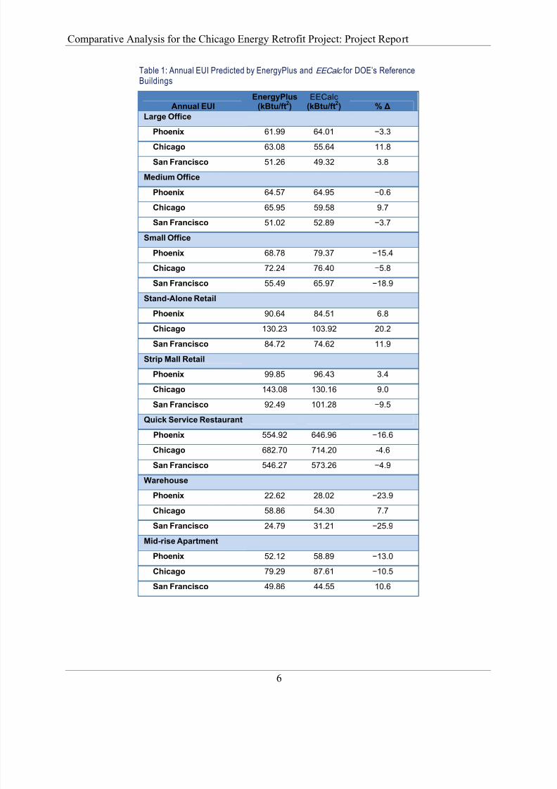
3 Comparison with EnergyPlus Predictions
To evaluate the capacity of the EECalc tool for retrofit analysis at a national scale, we compared EECalc predictions of energy consumption with those from EnergyPlus simulations. For this
analysis, we generated energy consumption estimates by using EECalc for a subset of DOE’s
reference buildings:
Large, medium, and small office buildings; a stand-alone retail building, a strip mall
retail building, a quick-service restaurant, a warehouse, and a mid-rise apartment;
Chicago, San Francisco, and Phoenix; and
Post-1980 construction.
Our objective for this exercise was not to prove that the EECalc predictions precisely matched
those from EnergyPlus simulations. EnergyPlus simulates heat transfer dynamically in buildings
at much greater detail and in much smaller time steps than the quasi-steady-state, monthlycalculations in EECalc. The translation of EnergyPlus input data into the significantly fewerinput parameters used by EECalc was in itself a challenge and potential source of differing
results. Other differences arose because the underlying models are not the same. As Figure 2
shows, there are differences, even between two versions of EnergyPlus, in the energyconsumption predictions for the DOE large office reference building in Chicago.
For the study, we compared EECalc results for the subset of reference buildings with theEnergyPlus Version 5 results that are posted on the DOE reference building website. We set out
to demonstrate that EECalc results matched reasonably well with EnergyPlus results and trended
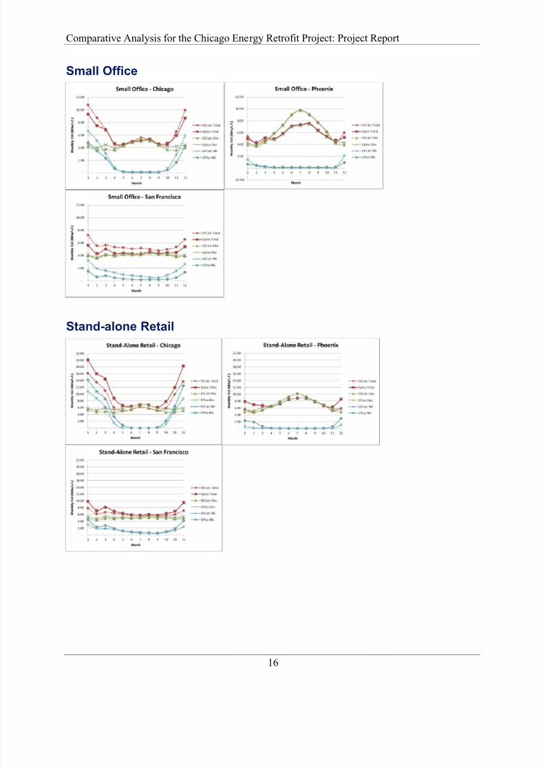
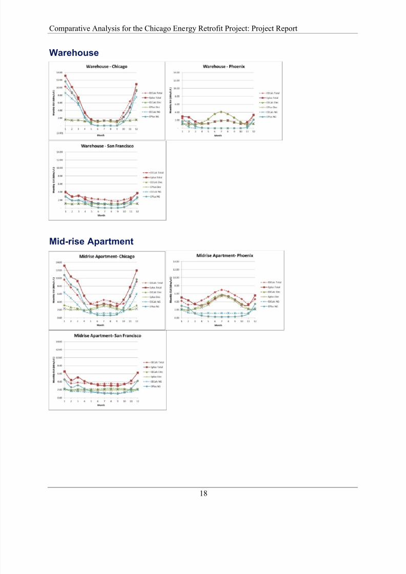
as would be expected from the physics of buildings. The results of the study are provided
graphically in Appendix A. The calculated annual EUIs (in kBtu/ft2
) from both tools are shownin Table 1.
Figure 2: Sensitivity of Energy Consumption Predictions to the Building Energy Model (Note the differencesin the EnergyPlus predicti ons between V5 and V7 versions of the sof tware using the same input f ile.)
8/13/2019 ANL DIS 14.2 Chicago Loop Comparative_Analysis_FINAL.docx
http://slidepdf.com/reader/full/anl-dis-142-chicago-loop-comparativeanalysisfinaldocx 16/59
Comparative Analysis for the Chicago Energy Retrofit Project: Project Report
6
Table 1: Annual EUI Predicted by EnergyPlus and EECalc for DOE’s ReferenceBuildings
Annual EUIEnergyPlus
(kBtu/ft2)
EECalc
(kBtu/ft2) % ∆
Large Office
Phoenix 61.99 64.01 −3.3
Chicago 63.08 55.64 11.8
San Francisco 51.26 49.32 3.8
Medium Office
Phoenix 64.57 64.95 −0.6
Chicago 65.95 59.58 9.7
San Francisco 51.02 52.89 −3.7
Small Office
Phoenix 68.78 79.37 −15.4
Chicago 72.24 76.40 −5.8
San Francisco 55.49 65.97 −18.9
Stand-Alone Retail
Phoenix 90.64 84.51 6.8
Chicago 130.23 103.92 20.2
San Francisco 84.72 74.62 11.9
Strip Mall Retail
Phoenix 99.85 96.43 3.4
Chicago 143.08 130.16 9.0
San Francisco 92.49 101.28 −9.5
Quick Service Restaurant
Phoenix 554.92 646.96 −16.6
Chicago 682.70 714.20 -4.6
San Francisco 546.27 573.26 −4.9
Warehouse
Phoenix 22.62 28.02 −23.9
Chicago 58.86 54.30 7.7
San Francisco 24.79 31.21 −25.9
Mid-rise Apartment
Phoenix 52.12 58.89−
13.0
Chicago 79.29 87.61 −10.5
San Francisco 49.86 44.55 10.6

8/13/2019 ANL DIS 14.2 Chicago Loop Comparative_Analysis_FINAL.docx
http://slidepdf.com/reader/full/anl-dis-142-chicago-loop-comparativeanalysisfinaldocx 17/59
Comparative Analysis for the Chicago Energy Retrofit Project: Project Report
7
Although there were a couple of cases in which the differences in the estimated energy use
predictions were greater than 20%, in general, the matches were reasonable. For the particularcase of warehouses in Phoenix and San Francisco, the energy use was so low that the models
were highly sensitive to slight variations in input parameters. We expect that with additional
effort to better translate the EnergyPlus detailed building information into EECalc inputs, the
differences would be further reduced. However, the point of the project is not to mirrorEnergyPlus predictions but to provide a credible, reliable method for assessing retrofit options.
For this purpose, the challenge is to overcome the recognized gap between model-predicted
consumption and actual energy consumption. Here, model precision and complexity have notclosed the gap. We have tackled the challenge by recognizing that uncertainty exists and then
reducing it through a novel Bayesian calibration process described in Appendix B.
3.1 Comparison with Data and Audits for Chicago Buildings
In our outreach efforts to building owners and energy consulting firms, we received mostly
positive feedback and enthusiasm about the concept and objectives of the project and EECalc tool. Organizations that subsequently agreed to collaborate by providing building data andenergy audit reports for the comparative study included the City of Chicago, CleanUrbanEnergy,
ComEd, Delta Institute, Merchandise Mart, Sieben Energy, Solomon Cordwell Buenz, Tishman-
Speyer, and U.S. Equities. Some of these data were received too late to be analyzed for thisreport.
In the end, we evaluated audit reports that included eQuest model results from five buildings
(Buildings A–E), an audit report using Integrated Environmental Solutions Virtual Environment(IES-VE) software from one building (Building F), EnergyPlus audit model results from three
buildings (Buildings G, H, and I), and measured energy use data from four buildings
(Buildings J, K, L, and M). For each building, we compiled and entered data on it into the EECalc tool to generate uncalibrated energy use predictions, then calibrated EECalc against
measured energy consumption data using Bayesian methods, as described in Appendix B. For
Buildings A–I, we also compared EECalc energy savings predictions with those reported in theenergy audits. The full analysis and results for each of the buildings analyzed are provided in
Appendix B.
A posit of the original EECalc research proposal was that the reduced number of input parameters for the calculation model and the ability to apply Bayesian calibration methods would
reduce the amount of data that needed to be collected for each building, which, in turn, would
reduce both the time and cost involved in producing a building energy efficiency audit, while
providing decision makers with energy savings predictions comparable in accuracy to moretraditional methods. This idea was confirmed by several examples that showed how the EECalc
calibration was able to identify the proper values for input parameters, which would normallyneed to be obtained through very detailed (and expensive) surveys. Further, we confirmed that
EECalc could accurately predict monthly utility usage with fairly low uncertainty on the basis ofonly a few known building input parameters.

8/13/2019 ANL DIS 14.2 Chicago Loop Comparative_Analysis_FINAL.docx
http://slidepdf.com/reader/full/anl-dis-142-chicago-loop-comparativeanalysisfinaldocx 18/59
Comparative Analysis for the Chicago Energy Retrofit Project: Project Report
8
3.1.1 Savings from Reduced Data Collection Requirements
As an example of how EECalc and Bayesian
calibration can reduce data collection and audit
needs, we highlight the case of Building D and
the estimation of building lighting loads here.Although lighting loads are important when
making energy assessments, they are notoriously
difficult to estimate because of the variable use,controls, and upgrades associated with individual
lighting units. For the Building D audit, an
extensive survey was undertaken to count thenumber of lighting fixtures and measure their
lighting power. From this survey, the lighting
power density (LPD) was determined to be
6.7 W/m2. In our calibration of EECalc plug and
lighting loads using measured submeteredelectricity consumption, we derived a mean value for the LPD of 7.8 W/m
2, as shown in
Figure 3. This comparable value was obtained without conducting an expensive lighting surveyand without using submetered data for individual lighting circuits. In addition, the result
quantified the expected uncertainty in lighting load (due to variable use and operation) that is
implicit in the measured data.
We also confirmed in this study that through calibration and use of informed default parameter
values, EECalc can provide good predictions for monthly and overall energy use on the basis of
very limited building data. Buildings E and F had energy audits that were highly redacted toensure the exact buildings could not be identified. The only information provided to us was the
building age; building height; general type of heating, ventilation, and air-conditioning (HVAC)unit; approximate extent of conditioned space; and a minimal description of the buildingenvelope. In short, the information we used in the analysis was no more than that required to
obtain an Energy Star rating for the building plus a general description of the building envelope.
Figure 4 shows results from the analysis of Building F. Monthly energy consumption predictions
from the uncalibrated and calibrated EECalc tool are compared to measured data. Even with the
very limited amount of building-specific input data, the uncalibrated EECalc predictionsmatched well with measured energy consumption data. The EECalc calibration further improved
the fit of the predictions to measured data as well as reducing the uncertainty associated with the
predictions (as shown by the narrower confidence intervals).
Figure 3: Comparison of the Initial LPDProbability Distrib ution (red dashes) and theCalibrated Posterior Distribution (solid bluehistogr am) (The red dashed line shows ou r initi alestimate of the LPD between 5 W/m2 and22 W/m2, with 13 W/m2 as the most probablevalue.)

8/13/2019 ANL DIS 14.2 Chicago Loop Comparative_Analysis_FINAL.docx
http://slidepdf.com/reader/full/anl-dis-142-chicago-loop-comparativeanalysisfinaldocx 19/59
Comparative Analysis for the Chicago Energy Retrofit Project: Project Report
9
Figure 4: Comparison o f Uncalibrated (left) and Calibrated (right ) EECalc Predictions ofMonthly EUI for Building F (There was very limited information for this building .)
3.1.2 Characterization of the Risk of Underperformance
Although most of the audit reports we studied were full of details, they all reported single valueestimates for energy savings associated with the proposed EEMs. When given these estimates,
the decision maker may still be uncertain about whether to invest in the retrofit. What is the
likelihood that the estimated energy savings will be realized? What is the probability that energycost savings will not cover the costs of the retrofit? Results from EECalc can help answer these
questions, as illustrated in Figure 5. Shown are energy savings for a chiller retrofit for Building E
(left) and a window retrofit for Building G (right) as predicted by EECalc and compared toestimates reported in the audit. The red curves are energy savings distributions predicted by
EECalc; the dashed vertical lines represent the energy savings estimates from the audits. For the
chiller retrofit for Building E, EECalc predicts a 70% chance that the actual energy savings will be less than determined by the audit. In the window retrofit for Building G, EECalc predicts a
28% chance that the actual energy savings will be lower than estimated or, alternatively, a 72%chance that the energy savings will be greater than estimated.
The EECalc results quantify the uncertainty in achievable energy savings, and hence the
investment risk of the retrofit, for the decision maker. Through EECalc analysis, uncertaintyabout energy savings estimates can be replaced with the confidence that a minimum energy
savings goal can be met.
Table 2 summarizes the data from all the audit comparisons. Although the energy savingsreported in the audits were mostly within the 95% confidence limits of EECalc predictions, they
were not necessarily near the EECalc-predicted means. As a “post-mortem” exercise, several
uncertainties could be at the root of the differences. For one, we do not know if the energysavings reported in the audit were those computed by using eQuest or came from expert
judgment informed by eQuest results. In addition, some assumptions regarding the input
parameters for EECalc had to be made in order to fill in gaps in the building data available fromthe audit reports. In the future, EECalc would be better tested if it were tested as part of active
audits rather than after the audits were completed.

8/13/2019 ANL DIS 14.2 Chicago Loop Comparative_Analysis_FINAL.docx
http://slidepdf.com/reader/full/anl-dis-142-chicago-loop-comparativeanalysisfinaldocx 20/59
Comparative Analysis for the Chicago Energy Retrofit Project: Project Report
10
Figure 5: EECalc Predictions of Energy Savings Distributions (red curve) and Audit ReportEstimates (blue point) for Building F Chiller Upgrade (left) and Building G Window Upgrade(right)
Table 2: Energy Savings Estimates from Energy Aud its and EECalc
Building Retrofit EEM
Annual EUIEECalc
(kBtu/ft2 /yr)
Energy SavingsAudit Estimate
(kBtu/ft2 /yr)
Energy SavingsEECalc Estimate
(kBtu/ft2 /yr)
A Boiler efficiency upgrade 56.8 10.3 11.7 +/− 2.6
B and C Supply & return fan variablefrequency drive (VFD)
60.7 1.6 2.1 +/− 0.7
D Lighting upgrade 117.7 2.4 5.7 +/− 3.9
Energy managementsystem (EMS) upgrade
0.3 1.6 +/− 1.3
E Chiller efficiency upgrade 75.7 6.0 3.3 +/− 2.1
Interior lighting upgrade 3.5 6.0 +/− 1.6
F Chiller efficiency upgrade 48.8 2.4 2.1 +/− 1.5
Demand based control 1.6 0.6 +/−
0.8
G Lighting upgrade 46.4 4.2 4.1 +/− 3.2
Window upgrade 7.3 8.1 +/− 2.5
H Chiller upgrade 42.1 3.3 2.5 +/− 1.2
Lighting control 1.7 2.5 +/− 0.7
I Chiller upgrade 73.3 2.2 2.0 +/− 1.4
Lighting control 7.8 8.4 +/− 3.4

8/13/2019 ANL DIS 14.2 Chicago Loop Comparative_Analysis_FINAL.docx
http://slidepdf.com/reader/full/anl-dis-142-chicago-loop-comparativeanalysisfinaldocx 21/59
Comparative Analysis for the Chicago Energy Retrofit Project: Project Report
11
4 Conclusions and Recommendations
This comparative study showed the general performance of the EECalc tool in predictingmonthly and annual building EUI by comparing predictions to measured EUI as well as its
performance in predicting the energy savings of various EEMs. The study validated EECalc’s
ability to make fairly accurate energy predictions with little information about the building, aswell as its ability to use Bayesian calibration to improve the estimates of important input
parameters, reducing the need for expensive and time-consuming audits. Finally, the study
showed EECalc’s ability to compute probabilities of EUI and energy savings for selected EEMs,allowing the characterization of the risk of underperformance of the selected retrofit.
The study results further validate the utility of the EECalc tool as a scalable, transparent, and
affordable platform for:
Benchmarking building energy performance;
Evaluating energy savings potential of energy efficiency technologies; and
Analyzing national, regional, and market impacts of energy efficiency initiatives,
strategies, codes, and standards.
Moving ahead, we note that the EECalc tool is now available as an Excel spreadsheet for energy
performance evaluation. Minor modifications are required to the tool to facilitate its use for
energy retrofit analysis. After these modifications are made, we propose to partner witharchitecture and engineering (A&E) firms and energy consultants who have agreed to pilot the
EECalc tool in parallel with their existing tools for their energy retrofit projects. These “live”
pilots will provide invaluable feedback to fine-tune the EECalc tool in preparation for a broader
deployment within the building energy services community.
We also propose to continue the development of retrofit analysis tools through three efforts:
1. Create the software code to automate the Bayesian calibration of the EECalc energy
results to individual building’s measured energy use data.
2. Pursue the development of the web-based energy efficiency investment decision tool,
EEInvest , which couples EECalc energy calculations with stochastic finance
calculations previously developed for the DBPD financial risk management tool.
3. Create EECalc tool versions specifically designed as decision tools to support DOE’sdeployment goals for specific DOE building technologies.

8/13/2019 ANL DIS 14.2 Chicago Loop Comparative_Analysis_FINAL.docx
http://slidepdf.com/reader/full/anl-dis-142-chicago-loop-comparativeanalysisfinaldocx 22/59
Comparative Analysis for the Chicago Energy Retrofit Project: Project Report
12
This page intentionally left blank.
8/13/2019 ANL DIS 14.2 Chicago Loop Comparative_Analysis_FINAL.docx
http://slidepdf.com/reader/full/anl-dis-142-chicago-loop-comparativeanalysisfinaldocx 23/59

8/13/2019 ANL DIS 14.2 Chicago Loop Comparative_Analysis_FINAL.docx
http://slidepdf.com/reader/full/anl-dis-142-chicago-loop-comparativeanalysisfinaldocx 24/59
Comparative Analysis for the Chicago Energy Retrofit Project: Project Report
14
This page intentionally left blank.

8/13/2019 ANL DIS 14.2 Chicago Loop Comparative_Analysis_FINAL.docx
http://slidepdf.com/reader/full/anl-dis-142-chicago-loop-comparativeanalysisfinaldocx 25/59
Comparative Analysis for the Chicago Energy Retrofit Project: Project Report
15
Appendix A: EnergyPlus Comparison Results
Table A-1: EnergyPlus Version 5 for Existing Buildings Constructed in or after 1980 (Results are from the followingweb site: http: //www1.eere.energy.gov/buildi ngs/commerc ial_initiative/after_1980.html.)
Large Office
Medium Officea
a The medium office had both electric reheat and gas heat. This version of EECalc allows for only once source of heating fuel,
and so it predicted higher natural gas consumption and lower electricity consumption than did EnergyPlus in the heating season.
8/13/2019 ANL DIS 14.2 Chicago Loop Comparative_Analysis_FINAL.docx
http://slidepdf.com/reader/full/anl-dis-142-chicago-loop-comparativeanalysisfinaldocx 26/59
Comparative Analysis for the Chicago Energy Retrofit Project: Project Report
16
Small Office
Stand-alone Retail

8/13/2019 ANL DIS 14.2 Chicago Loop Comparative_Analysis_FINAL.docx
http://slidepdf.com/reader/full/anl-dis-142-chicago-loop-comparativeanalysisfinaldocx 27/59
Comparative Analysis for the Chicago Energy Retrofit Project: Project Report
17
Strip Mall Retail
Quick-service Restaurant
8/13/2019 ANL DIS 14.2 Chicago Loop Comparative_Analysis_FINAL.docx
http://slidepdf.com/reader/full/anl-dis-142-chicago-loop-comparativeanalysisfinaldocx 28/59
Comparative Analysis for the Chicago Energy Retrofit Project: Project Report
18
Warehouse
Mid-rise Apartment

8/13/2019 ANL DIS 14.2 Chicago Loop Comparative_Analysis_FINAL.docx
http://slidepdf.com/reader/full/anl-dis-142-chicago-loop-comparativeanalysisfinaldocx 29/59
Comparative Analysis for the Chicago Energy Retrofit Project: Project Report
19
Appendix B: EECalc Calibrations and Predictions
We apply Bayesian inference as a new approach for calibrating and factoring uncertainty into building energy models, including the EECalc tool. Bayesian calibration is an alternative to
traditional, expert-intensive approaches that require “tweaking” of energy model input
parameters to match measured data. Bayesian statistical methods instead derive the most likelydistributions (posterior distributions) of input parameters from their predefined probability
density functions (i.e., prior distributions) to explain the measured energy use data. The resulting
posterior distributions are then used in Monte Carlo samplings of the energy model to yield probabilistic outcomes of predicted energy savings.
The Bayesian paradigm treats a probability as a numerical estimate of the degree of belief in a
hypothesis. Under this paradigm, our prior belief in the true values of calibration parameters is
quantified as prior density functions p( θ ). The prior distributions are updated (given measureddata on building performance) through the likelihood function p(y|θ ). The likelihood function
compares how closely model outcomes with testing parameter values match the measured data.
As the result of Bayesian calibration, we obtain posterior distributions of calibration parameters p( θ |y):
p( θ |y)∝ p( θ )×p(y|θ )
where the symbol ∝ denotes proportionality. After the Bayesian process is completed, theresulting likelihood function is scaled so that the function is a true probability density function.
The Bayesian calibration module requires three major steps: (1) specification of prior probability
distributions for uncertain parameters, (2) formulation of the likelihood function, and
(3) application of the Markov chain Monte Carlo (MCMC) method for posterior simulation. We
quantify prior distributions on the basis of expert knowledge developed through reviewingtechnical papers and industry reports. We formulate the likelihood function as the Gaussian
process model, following the Bayesian framework of Kennedy and O’Hagan (2001). To
approximate posterior distributions from one joint multivariate distribution p( θ )× p(y|θ ), weapply one of the MCMC methods: the Metropolic-Hastings method. The method explores the
parameter space in an iterative manner and accepts those steps that satisfy an acceptance
criterion (Gelman et al. 2004). As a result, the Bayesian calibration module provides a set ofaccepted parameter values as posterior distributions. The calibration process is described in more
detail in Heo et al. (2012).
Building A
Building A is a 28-story, high-rise tower with concrete panel cladding that was completed in
1971. It has a conditioned floor space of 392,000 ft2 (36,431 m
2). It uses gas boiler and domestic
hot water heating and electric centrifugal chillers for cooling. The windows are first-generation,insulated, glazing units with a fairly dark tint. The roofing was recently replaced, and insulation
was added to bring the roof to R20. The lighting is a mixture of T12, T8, T5, and compact
fluorescent light (CFL) with an estimated LPD of 0.9 W/ft2 (10 W/m
2). Billing data were

8/13/2019 ANL DIS 14.2 Chicago Loop Comparative_Analysis_FINAL.docx
http://slidepdf.com/reader/full/anl-dis-142-chicago-loop-comparativeanalysisfinaldocx 30/59
Comparative Analysis for the Chicago Energy Retrofit Project: Project Report
20
provided for the 2008 calendar year. One important note is that tenant electric loads (lighting and
equipment plug loads) were billed directly to the tenant, and so the measured billing data do notinclude the tenant loads. The auditors estimated that 90% of the total building electrical lighting
and plug loads were billed to the tenants but contributed to the heating and cooling load of the
building HVAC system. To calibrate the eQuest energy model, the auditors had to add the
unbilled electric loads back into the heating and cooling loads of the building. For the sake ofconsistency and comparison, we opted to model tenant electricity usage in the same manner,
although a variation of the fraction with season is probably more appropriate. Using the total
estimated building electric consumption, the overall building EUI was estimated to be57 kBtu/ft
2 (178 kWh/m
2).
The building audit we received was not a formal ASHRAE (American Society for Heating,Refrigerating, and Air-Conditioning Engineers) level 2 audit. In addition, it focused on small
retrofits with only one major retrofit – a boiler upgrade to replace the aging original boilers. The
auditors created and calibrated an eQuest model for the building and used it for estimating the
energy savings from upgrading the boiler to a high-performance condensing gas boiler. The
existing boilers were estimated to have an efficiency of about 60%. The predicted energy savingsfrom the boiler upgrade was 40,665 therms/yr, which converts to a savings of 10.4 kBtu/ft2
(30.4 kWh/m2).
Figure BA-1 compares energy consumption data calculated by the uncalibrated EECalc model
against measured data from the utility bills and results from the eQuest modeling conducted bythe energy auditor. Without calibration, the tool estimates monthly gas consumption data that
closely match measured data. However, the tool estimates electricity consumption data
differently than the measured data: It overpredicts electricity consumption during the summerand underpredicts electricity consumption during the winter when compared with the measured
data. The difference can arise from incorrect parameter values estimated on the basis of drawingsand specifications. Calibration can enhance the reliability of the model by tuning highly
uncertain parameters (due to lack of information) with of utility bill data.
Figure B.A-1: Energy Consumpti on Data for Building A Predicted by the Uncalibrated EECalc andCalibrated eQuest in Comparison wi th Measured Data
0 2 4 6 8 10 120
5
10
15
20
25
30
35
40
Month
G a
s C o n s u m p t i o n ( k W h / m 2 )
0 2 4 6 8 10 120
1
2
3
4
5
6
7
8
9
10
Month
E l e c t r i c i t y C o n s u m p t i o n ( k W h / m 2 )
Uncalibrated EECalc
Calibrated eQuest
Utility Data

8/13/2019 ANL DIS 14.2 Chicago Loop Comparative_Analysis_FINAL.docx
http://slidepdf.com/reader/full/anl-dis-142-chicago-loop-comparativeanalysisfinaldocx 31/59
Comparative Analysis for the Chicago Energy Retrofit Project: Project Report
21
Before calibration, we applied the Morris method to identify the dominant uncertain parameters
with respect to their effect on gas and electricity consumption. Since we used both gas andelectricity bills for calibration, we ranked uncertainty parameters separately with respect to item
consumed and selected the top two parameters in each ranking list. The selected parameters for
calibration were (1) plugload–occupied, (2) cooling system mean partial load value (MPLV),
(3) infiltration rate, and (4) heating system efficiency.
Figure BA-2 shows calibration results in the form of probability distributions. The red dashed
line indicates prior beliefs about true parameter values, and the blue histogram indicates a probability of true values updated through the calibration process. For plugload–occupied, the
expected value does not change from our prior estimate, but the magnitude of uncertainty is
greatly reduced. For the cooling system MPLV, the expected value changes from 0.7 to 0.9. Forinfiltration rate, the results suggest that the building envelope is most likely leakier than expected.
For the heating system efficiency, the posterior distribution does not change much from the prior
distribution.
Figure B.A-2: Calibration Results for Building A (red dashed line = prior , blue histogram= posterior d istribution)
Figure BA-3 displays the baseline energy consumption data predicted by the calibrated EECalc model compared with eQuest results and measured data. The calibrated model results in much
narrower confidence intervals for predictions than does the uncalibrated model. This comparison
demonstrates that Bayesian calibration enhances the reliability of the baseline model by
5 10 15 20 25 30 350
500
1000
1500
2000
2500
3000
3500
4000
4500
Plugload - Occupied (W2/m2)
0.4 0.5 0.6 0.7 0.8 0.9 1 1.1 1.2 1.30
500
1000
1500
2000
2500
3000
Cool System MPLV
1 2 3 4 5 6 7 8 9 100
500
1000
1500
2000
2500
3000
3500
4000
Infiltration Rate (m3/h/m2 @75Pa)
0 .5 0.52 0.54 0.56 0 .58 0 .6 0 .62 0.64 0.66 0 .68 0.70
500
1000
1500
2000
2500
3000
3500
Heating System Efficiency

8/13/2019 ANL DIS 14.2 Chicago Loop Comparative_Analysis_FINAL.docx
http://slidepdf.com/reader/full/anl-dis-142-chicago-loop-comparativeanalysisfinaldocx 32/59
Comparative Analysis for the Chicago Energy Retrofit Project: Project Report
22
improving its fit to measured data and reducing its uncertainty. Although the calibrated model
quite closely replicates actual energy consumption, it still results in a discrepancy between predicted electricity consumption and actual consumption during the winter. This discrepancy
can be at least partially attributed to the inability of the monthly EECalc model to capture
cooling loads that occur during peak hours during the winter and the intermittent season.
Figure B.A-3: Energy Consumpti on Data for Building A Predicted by the Calibrated EECalc and theCalibrated eQuest in Comparison w ith Measured Data
The audit project evaluated upgrading a boiler from an efficiency of 0.60 to 0.95, using aneQuest model under typical meteorological year (TMY) weather conditions. In our analysis
process, we propagated uncertainty in the model quantified by the Bayesian approach and
additional uncertainty from the retrofit option (ranging between 0.90 and 0.97). By subtracting post-retrofit energy consumption data from baseline energy consumption data, we obtained
probabilistic outcomes of annual energy savings. Figure BA-4 shows a plausible range of annual
energy savings and their likelihoods calculated by the proposed method in comparison with the
deterministic value predicted by the typical audit project with the eQuest model. The single valueobtained by using the eQuest model slightly underpredicts the effect of the retrofit intervention in
comparison with the expected value by the EECalc model.
Figure B.A-4: Probability Distribution for Building A of Annual Energy Savingsfrom Bo iler Upgrade. Red line is t he EECalc savings prediction and the bluedashed line is the eQuest saving prediction. These results can be compared to theoverall annual use of the building , which was estimated by eQuest to be144 kWh/m2.
0 2 4 6 8 10 120
5
10
15
20
25
30
35
40
Month
G a s C o n s u m p t i o n ( k W h / m 2 )
0 2 4 6 8 10 120
1
2
3
4
5
6
7
8
9
10
Month
E l e c t r i c i t y C o n s u m p t i o n ( k W h / m 2 )
Calibrated EECalc
Calibrated eQuest
Utility Data
20 25 30 35 40 45 50 550
0.01
0.02
0.03
0.04
0.05
0.06
0.07
0.08
0.09
0.1
Boiler Upgrade Annual Energy Saving (kWh/m2)
P r o b a b i l i t y
Risk of Underperformance
15.6%

8/13/2019 ANL DIS 14.2 Chicago Loop Comparative_Analysis_FINAL.docx
http://slidepdf.com/reader/full/anl-dis-142-chicago-loop-comparativeanalysisfinaldocx 33/59
Comparative Analysis for the Chicago Energy Retrofit Project: Project Report
23
Buildings B and C
Buildings B and C are two buildings that share parts of the HVAC system, have some common
utility billing, and are conjoined by a 15-story common space. Because of the systems and billing
overlaps, we analyzed the complex as a single large building. The buildings are stone panel
curtain wall high-rises with a combined conditioned area of 2,880,000 ft2
(268,000 m2
). Thetaller building is 60 stories tall, and the shorter building is 35 stories tall. The buildings were
completed in 1989 and 1992, respectively. Glazing is standard double-insulated glazing fromabout 1990 with a fairly dark tint. The building is heated by electric boilers and is cooled by
centrifugal electric chillers, both of which are original to the building. The building has a
building automation system (BAS) that is used for monitoring building operation and central
control of the building HVAC setpoints, but automatic controls and fault detection anddiagnostics (FDD) are not implemented. In 2011, the building had an EUI of 75 kBtu/ft
2
(237 kWh/m2).
An ASHRAE level 2 audit was performed on the building, which included development of an
eQuest model that was used for EEM savings estimation. Most of the EEMs suggested in theaudits were small upgrades to individual lighting elements (exit lighting, occupancy sensors on bathroom only). An upgrade of the supply and return fans to variable frequency drive (VFD) was
one of the larger upgrades suggested. That EEM was chosen for comparison.
Figure BBC-1 compares electricity consumption data calculated by the uncalibrated EECalc tool
with measured data from utility bills in 2010 and results from the eQuest model (from the audit
project). Without calibration, the tool underpredicted electricity consumption for most of the
months except the winter season.
Figure B.B&C-1: Energy Consumpt ion Data for Buil dings B and C Predicted by theUncalibrated EECalc and Calibrated eQuest in Comparison wi th Measured Data
Based on the ranking of model parameters from the Morris method, we selected the top four for
calibration: (1) infiltration rate, (2) plugload–occupied, (3) LPD, and (4) heating temperaturesetpoint. Figure B.B&C-2 exhibits posterior distributions of the calibration parameters updated
from prior distributions. Overall, uncertainty in the plausible range of parameter values was not
0 2 4 6 8 10 120
5
10
15
20
25
30
35
40
45
50
Month
E l e c t r i c i t y C o n s u m p t i o n ( k W h / m
)
Uncalibrated EECalcCalibrated eQuest
Utility Data
8/13/2019 ANL DIS 14.2 Chicago Loop Comparative_Analysis_FINAL.docx
http://slidepdf.com/reader/full/anl-dis-142-chicago-loop-comparativeanalysisfinaldocx 34/59
Comparative Analysis for the Chicago Energy Retrofit Project: Project Report
24
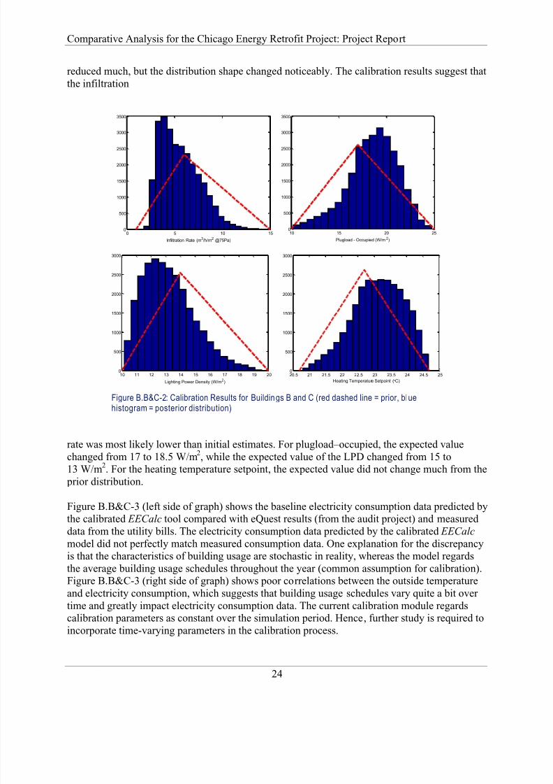
reduced much, but the distribution shape changed noticeably. The calibration results suggest that
the infiltration
Figure B.B&C-2: Calibration Results for Buildings B and C (red dashed line = prior, bl ue
histogram = posterior distribution)
rate was most likely lower than initial estimates. For plugload–occupied, the expected value
changed from 17 to 18.5 W/m2, while the expected value of the LPD changed from 15 to
13 W/m2. For the heating temperature setpoint, the expected value did not change much from the
prior distribution.
Figure B.B&C-3 (left side of graph) shows the baseline electricity consumption data predicted bythe calibrated EECalc tool compared with eQuest results (from the audit project) and measured
data from the utility bills. The electricity consumption data predicted by the calibrated EECalc
model did not perfectly match measured consumption data. One explanation for the discrepancyis that the characteristics of building usage are stochastic in reality, whereas the model regards
the average building usage schedules throughout the year (common assumption for calibration).Figure B.B&C-3 (right side of graph) shows poor correlations between the outside temperature
and electricity consumption, which suggests that building usage schedules vary quite a bit over
time and greatly impact electricity consumption data. The current calibration module regardscalibration parameters as constant over the simulation period. Hence, further study is required to
incorporate time-varying parameters in the calibration process.
0 5 10 150
500
1000
1500
2000
2500
3000
3500
Infiltration Rate (m3/h/m2 @75Pa)
10 15 20 250
500
1000
1500
2000
2500
3000
3500
Plugload - Occupied (W/m2)
10 11 12 13 14 15 16 17 18 19 200
500
1000
1500
2000
2500
3000
Lighting Power Density (W/m2)
20.5 21 21.5 22 22.5 23 23.5 24 24.5 250
500
1000
1500
2000
2500
3000
Heating Temperature Setpoint (C)

8/13/2019 ANL DIS 14.2 Chicago Loop Comparative_Analysis_FINAL.docx
http://slidepdf.com/reader/full/anl-dis-142-chicago-loop-comparativeanalysisfinaldocx 35/59
Comparative Analysis for the Chicago Energy Retrofit Project: Project Report
25
Figure B.B&C-3: Energy Consumpt ion Data for Buil dings B and C Predicted by the Calibrated EECalc andCalibrated eQuest in Comparison wi th Measured Data (left), and Scatter Plot o f Monthly Average OutsideTemperatures and Electricity Consumption (right)
The audit project evaluated the installation of VFDs on supply and return fans, using an eQuest
model under TMY weather conditions. Figure B.B&C-4 shows a probability distribution ofannual energy savings predicted by the calibrated EECalc model in comparison with the single
value of annual energy savings documented in the audit report. EECalc results suggest that the
expected energy savings are likely to be higher than the audit estimate.
Figure B.B&C-4: Probability Distribution for Buildings B and C of Annual EnergySavings from Fan VFDs. Red line is the EECalc savings prediction and the bluedashed line is the eQuest saving prediction. These results can be compared to the
overall annual use of the building which was estimated by eQuest to be190 kWh/m2.
0 2 4 6 8 10 120
5
10
15
20
25
30
35
40
45
50
Month
E l e c t r i c i t y C o n s u m p t i o n ( k W h / m 2 )
Calibrated EECalc
Calibrated eQuest
Utility Data
-10 -5 0 5 10 15 20 25 304
4.5
5
5.5
6
6.5
7x 10
6
Monthly Average Outside Temperature (C)
M o n t h l y E l e c t r i c i t y C o n s u m p t i o n ( k W h / m 2 )
2 3 4 5 6 7 8 9 10 11 120
0.05
0.1
0.15
0.2
0.25
0.3
0.35
Fan VFDs Annual Energy Saving (kWh/m2)
P r o b a b i l i t y
Risk ofUnderperformance
6.9%

8/13/2019 ANL DIS 14.2 Chicago Loop Comparative_Analysis_FINAL.docx
http://slidepdf.com/reader/full/anl-dis-142-chicago-loop-comparativeanalysisfinaldocx 36/59
Comparative Analysis for the Chicago Energy Retrofit Project: Project Report
26
Building D
Building D is a 28-story, steel and glass high rise completed in 1963. It has a conditioned space
of 1,540,000 ft2 (143,287 m
2). The building was designed to be used primarily as a courthouse
and civic center and has an extremely high floor-to-floor span of 19.7 ft (6 m). Because of the
many civic center functions that occur in the open space outside the building, some electricityand hot water use patterns are very abnormal. The building HVAC system also provides hot and
cold water for another nearby building. Finally the building houses a small data center(approximately 460 kW) for which electricity is billed separately, but which contributes to the
cooling load of the building. Because of the potentially high occupancy of the building, the
HVAC system is designed to provide extremely high ventilation rates: five times higher than the
standard ventilation rate used for offices. As a result, the fan power loss factors are quiteuncertain, offering a good opportunity to show the power of Bayesian calibration to reduce
uncertainty. In addition, the ventilation system is a combination of constant air volume (CAV)
and variable air volume (VAV) as part of the air handling system has been upgraded during the buildings lifetime. The heating and hot water are provided by gas boilers and cooling is provided
by centrifugal chillers.
The building audit was extremely thorough and well conducted. Submetering of lighting and
plugloads was installed. A full (and expensive) lighting audit was conducted to determine the
true connected lighting load. A comparison of EECalc results to these audit data offered theopportunity to see how the Bayesian calibration methods of EECalc can accurately estimate the
same lighting load with far less effort. Of the audit recommendations, two were appropriate to be
modeled with EECalc: lighting upgrades and upgrades/optimization of the Energy Management
System (EMS). The lighting upgrades included the addition of occupancy sensors, daylightingcontrols, and the reduction of the lighting load. The EMS upgrade included development of an
optimized fan/chiller startup sequence, additional set point control, and online diagnostics to
detect abnormal building operation. We will compare EECalc energy savings predictions tothese two EEM.
This building has submetered electricity consumption for appliances and lighting in addition tototal electricity and gas utility bills. In order to fully exploit measured data available in the
calibration process, we conducted a two-step calibration process: (1) calibrating part of the
EECalc model relevant to the submetered data and (2) calibrating the whole EECalc model using
the total utility bills.
As the first step, we calibrated a subset of model parameters for plugload and lighting against the
submetered data: (1) plugload–occupied, (2) LPD, and (3) fraction of lighting on while occupied.
Figure B.D-1 shows the posterior distributions of the three parameters refined from the priordistributions. For plugload and LPD, the results indicate that actual power densities were most
likely to be much lower than the prior estimates, and uncertainty was greatly reduced. The audit project conducted an extensive survey to count the number of lighting fixtures and to instantly
measure their lighting powers. From this survey, it was determined that the LPD was 6.7 W/m2, a
value close to the expected value (7.9) from the calibration. By calibrating the submodel of
plugload and lighting with submeter data but without completing an extremely expensive survey,
we can adequately derive the lighting baseline that matches the survey result well. For the
8/13/2019 ANL DIS 14.2 Chicago Loop Comparative_Analysis_FINAL.docx
http://slidepdf.com/reader/full/anl-dis-142-chicago-loop-comparativeanalysisfinaldocx 37/59
Comparative Analysis for the Chicago Energy Retrofit Project: Project Report
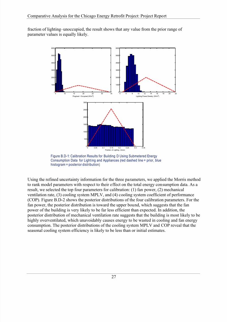
27
fraction of lighting–unoccupied, the result shows that any value from the prior range of
parameter values is equally likely.
Figure B.D-1: Calibration Results for Building D Using Submetered EnergyConsumption Data for Light ing and Appliances (red dashed line = prior, bluehistogram = posterior distribution)
Using the refined uncertainty information for the three parameters, we applied the Morris method
to rank model parameters with respect to their effect on the total energy consumption data. As a
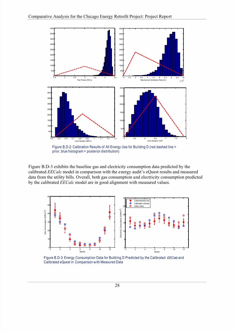
result, we selected the top four parameters for calibration: (1) fan power, (2) mechanical
ventilation rate, (3) cooling system MPLV, and (4) cooling system coefficient of performance(COP). Figure B.D-2 shows the posterior distributions of the four calibration parameters. For the
fan power, the posterior distribution is toward the upper bound, which suggests that the fan power of the building is very likely to be far less efficient than expected. In addition, the
posterior distribution of mechanical ventilation rate suggests that the building is most likely to be
highly overventilated, which unavoidably causes energy to be wasted in cooling and fan energy
consumption. The posterior distributions of the cooling system MPLV and COP reveal that theseasonal cooling system efficiency is likely to be less than or initial estimates.
5 10 15 20 25 30 350
1000
2000
3000
4000
5000
6000
Plugload - Occupied (W/m2)
4 6 8 10 12 14 16 18 20 220
1000
2000
3000
4000
5000
6000
Lighting Power Density (W/m2)
0 0.05 0.1 0.15 0.2 0.25 0.3 0.350
500
1000
1500
2000
2500
3000
Fraction of Lighting -Unocc
8/13/2019 ANL DIS 14.2 Chicago Loop Comparative_Analysis_FINAL.docx
http://slidepdf.com/reader/full/anl-dis-142-chicago-loop-comparativeanalysisfinaldocx 38/59
Comparative Analysis for the Chicago Energy Retrofit Project: Project Report
28
Figure B.D-2: Calibration Results of All Energy Use for Bui lding D (red dashed line =prior, blue histogram = posterior distribution)
Figure B.D-3 exhibits the baseline gas and electricity consumption data predicted by thecalibrated EECalc model in comparison with the energy audit’s eQuest results and measured
data from the utility bills. Overall, both gas consumption and electricity consumption predicted
by the calibrated EECalc model are in good alignment with measured values.
Figure B.D-3: Energy Consumpt ion Data for Build ing D Predicted by the Calibrated EECalc andCalibrated eQuest in Comparison w ith Measured Data
1.5 2 2.5 3 3.5 4 4.50
500
1000
1500
2000
2500
3000
3500
4000
4500
Fan Power (W/l.s)
5 5.5 6 6.5 7 7.5 8 8.5 9 9.5 10
x 105
0
500
1000
1500
2000
2500
3000
3500
4000
4500
Mechanical Ventilation Rate (l/s)
0.4 0.5 0.6 0.7 0.8 0.9 1 1.1 1.2 1.30
500
1000
1500
2000
2500
3000
3500
4000
4500
Cool System MPLV
5 5.5 6 6.5 7 7.5 80
500
1000
1500
2000
2500
3000
Cool System COP
0 2 4 6 8 10 120
10
20
30
40
50
60
Month
G a
s C o n s u m p t i o n ( k W h / m 2 )
0 2 4 6 8 10 120
5
10
15
20
25
30
Month
E l e c t r i c i t y C o n s u m p t i o n ( k W h / m 2 )
Calibrated EECalc
Calibrated eQuest
Utility Data

8/13/2019 ANL DIS 14.2 Chicago Loop Comparative_Analysis_FINAL.docx
http://slidepdf.com/reader/full/anl-dis-142-chicago-loop-comparativeanalysisfinaldocx 39/59
Comparative Analysis for the Chicago Energy Retrofit Project: Project Report
29
The audit project evaluated (1) upgrading lighting to high-efficiency T8 lighting systems and
(2) upgrading the EMS to optimize control schedules. Figure B.D-4 displays a probabilitydistribution of annual energy savings per EEM against a single value of energy savings from the
audit report. The comparison indicates that energy savings are likely to be much higher than the
estimated values documented in the audit report.
Figure B.D-4: Probability Distributions for Building D of Annual Energy Savings from LightingUpgrade (left) and EMS Upgrade (right). Red line i s EECalc savings predict ion, blue dashed line iseQuest saving predicti on. These results can be compared to the overall annual use of the build ingwhich was estimated by eQuest to be 371 kWh/m2
Building E
This building is one of three buildings for which the building audits were highly redacted for
confidentiality reasons. The three buildings offer the opportunity to evaluate the overall energy
use and EEM savings predictions from EECalc when only very limited building information was
available. Building E is over 40 stories tall, with a floor area in excess of 1,000,000 ft2
(100,000 m2). It was built before 1975. The building has original HVAC chillers, electric boilers,
and first-generation insulated glazing units and a 130-kW exterior lighting load.
For this building, we assumed a 2:1 aspect ratio for the building depth-to-width ratio. From this
ratio, the building height and building envelope size (wall size and roof size) were estimated.
Assuming a 40% vision glazing fraction (as was common for a 1970s-era, glass, high-rise office),window and opaque wall areas were estimated. Based on common construction techniques from
the year that the building was built, the U value for the walls and the U and solar heat gain
coefficient (SHGC) values for the window were estimated. The roof was assumed to have beenreplaced sometime between 1990 and 2000, and it was assumed additional insulation was used to
bring the roof to R15. Since the chillers and boilers were original to the building, equipment
efficiencies were estimated. Standard office operating schedules and heating/cooling efficiencies
were assumed. Because the chillers and boilers were original, it was assumed that there was noBAS, or, if there was one, it was not being used for highly automated control.
-5 0 5 10 15 20 25 30 35 40 450
0.01
0.02
0.03
0.04
0.05
0.06
Lighting Upgrade Annual Energy Saving (kWh/m2)
P r o b a b i l i t y
Risk ofUnderperformance
3.7%
-2 0 2 4 6 8 10 12 140
0.02
0.04
0.06
0.08
0.1
0.12
0.14
0.16
0.18
EMS Upgrade Annual Energy Saving (kWh/m2)
P r o b a b i l i t y
2.7%

8/13/2019 ANL DIS 14.2 Chicago Loop Comparative_Analysis_FINAL.docx
http://slidepdf.com/reader/full/anl-dis-142-chicago-loop-comparativeanalysisfinaldocx 40/59
Comparative Analysis for the Chicago Energy Retrofit Project: Project Report
30
The audit was an ASHRAE level 2 audit. A building energy model was created in eQuest that
was used to evaluate the larger EEM suggestions. We will compare the EECalc results to theinterior lighting upgrades and chiller replacement/upgrades suggested in the audit.
Figure B.E-1 compares energy consumption data calculated by the uncalibrated EECalc tool
against measured data from the utility bills and results from the eQuest modeling from the auditreport. Without calibration, the tool overestimates total electricity consumption data, especially
during the winter, when compared with the measured consumption data. This overestimation can
be simply due to overestimated parameter values in the base EECalc model, which will becorrected through the calibration process.
Figure B.E-1: Energy Consumpti on Data for Build ing E Predicted by theUncalibrated EECalc and Calibrated eQuest in Comparison wi th Measured Data
Based on the ranking of model parameters from the Morris method, we selected the top four parameters: (1) wall U value, (2) infiltration rate, (3) heating temperature setpoint, and (4) LPD.Figure B.E-2 shows probability distributions of the four parameters as the result of the Bayesian
calibration process. The actual wall U value is very likely to be lower than our initial estimate,
which suggests that the building envelope is more insulated than our initial estimate. For theinfiltration rate, the expected value changes from 3.5 to 2 m
3/h/m
2 at 75 Pa, which suggests the
building envelope is more air-tight than we initially estimated. For the heating temperaturesetpoint, the expected value did not change much from the prior estimate. For the LPD, the
expected value shifted from 10 to 12 W/m2, which reveals that the lighting consumes more
energy than our initial estimate showed.
0 2 4 6 8 10 120
10
20
30
40
50
60
70
Month
E l e c t r i c i t y C o n s u m
p t i o n ( k W h / m
)
Uncalibrated EECalc
Calibrated eQuest
Utility Data

8/13/2019 ANL DIS 14.2 Chicago Loop Comparative_Analysis_FINAL.docx
http://slidepdf.com/reader/full/anl-dis-142-chicago-loop-comparativeanalysisfinaldocx 41/59
Comparative Analysis for the Chicago Energy Retrofit Project: Project Report
31
Figure B.E-2: Calibration Results for Building E (red dashed line = prior, blue histog ram =posterior distribution)
Figure B.E-3 displays the baseline energy consumption data predicted by the calibrated EECalc model compared with eQuest results and the measured consumption data. After the calibration,
the EECalc model predictions were in good alignment with the measured consumption data, withgreatly reduced confidence intervals. The calibrated eQuest model underpredicted electricityconsumption during the winter.
Figure B.E-3: Energy Consumpt ion Data for Build ing E Predicted by the CalibratedEECalc and the Calibrated eQuest in Comparison with Measured Data
2 2.5 3 3.5 4 4.5 50
500
1000
1500
2000
2500
3000
3500
Wall U value (W/m2.K)
0 1 2 3 4 5 60
500
1000
1500
2000
2500
3000
Infiltration Rate (m3/h/m2 @75Pa)
19 19.5 20 20.5 21 21.5 22 22.5 230
500
1000
1500
2000
2500
3000
Heating Temp Setpoint (C)
5 6 7 8 9 10 11 12 13 14 150
500
1000
1500
2000
2500
3000
3500
4000
Lighting Power Density (W/m2)
0 2 4 6 8 10 120
10
20
30
40
50
60
70
Month
E l e c t r i c i t y C o n s u m p t i o n ( k W h / m
)
Calibrated EECalc
Calibrated eQuest
Utility Data

8/13/2019 ANL DIS 14.2 Chicago Loop Comparative_Analysis_FINAL.docx
http://slidepdf.com/reader/full/anl-dis-142-chicago-loop-comparativeanalysisfinaldocx 42/59
Comparative Analysis for the Chicago Energy Retrofit Project: Project Report
32
We evaluated two EEMs from the audit report: (1) upgrading a chiller’s efficiency from 4.0 to
7.0 and (2) upgrading interior lighting. Figure B.E-4 shows probability distributions of annualenergy savings per EEM. Relative to EECalc predictions, energy savings estimated in the audit
were likely to be less for the chiller upgrade and more for the lighting upgrade.
Figure B.E-4: Probability Distributions for Building E of Annual Energy Savings
from Chill er Upgrade (left) and Interior Li ghting Uupgrade (right). Red line is theEECalc savings predict ion and the blue dashed line is the eQuest savingprediction . These results can be compared to the overall annual use of thebuilding which was estimated by eQuest to be 239 kWh/m2.
Building F
This is another of the buildings with the highly redacted audits. Building F is over 30 stories tall
of mixed retail and office space with over 400,000 ft2 (40,000 m
2) of conditioned floor space and
was built before 1975. The building is a concrete panel curtain wall construction with first
generation insulated glazing original to the building. HVAC is electric chillers with electric boilers and electric baseboard heating, all original to the building. All HVAC equipment isconstant speed and air delivery is via a CAV system. For this building, a 1.5:1 side ratio with 40%
glazing ratio was assumed. This information was used to estimate opaque wall and window sizes.From knowledge of the year of build, the U value for the walls and the U and SHGC values for
the windows were estimated. The roof was assumed to have been replaced sometime between
1990 and 2000 and additional insulation to bring the roof to R15 was assumed. Since the chillersand boilers were original to the building, equipment efficiencies were estimated. Standard office
operating schedules and heating/cooling efficiencies were assumed. Because the chillers and
boilers were original, it was assumed that there was no BAS, or, if there was one, it was not being used for highly automated control.
The audit was an ASHRAE level 2. An Integrated Environmental Solutions Virtual Environment
(IES-VE) model and custom software of the auditors was used for estimating EEM savings, but amonthly estimate of energy use was not presented. Of the suggested EEMs, we modeled two: a
chiller replacement/upgrade and the conversion of the CAV system to a demand-control
ventilation system.
0 5 10 15 20 25 300
0.02
0.04
0.06
0.08
0.1
0.12
Chiller Upgrade Annual Energy Saving (kWh/m 2)
P r o b a b i l i t y
98.4%
-5 0 5 10 15 20 25 30 35 400
0.01
0.02
0.03
0.04
0.05
0.06
0.07
0.08
0.09
Interior Lighting Upgrade Annual Energy Saving (kWh/m2)
P r o b a b i l i t y
6.6%

8/13/2019 ANL DIS 14.2 Chicago Loop Comparative_Analysis_FINAL.docx
http://slidepdf.com/reader/full/anl-dis-142-chicago-loop-comparativeanalysisfinaldocx 43/59
Comparative Analysis for the Chicago Energy Retrofit Project: Project Report
33
Figure B.F-1 compares energy consumption data calculated by the uncalibrated EECalc tool
against measured data from the utility bills. Without calibration, the tool still calculated the totalelectricity consumption data close to measured data, although it slightly overpredicted the
consumption data throughout the year. The magnitude of uncertainty in predictions was quite
large, especially for the winter season.
Figure B.F-1: Energy Consumption Data for Buildi ng F Predicted by theUncalibrated EECalc in Comparison with Measured Data
Through the Morris method, we ranked model parameters in terms of their effect on energy
consumption data, and selected the top four parameters: (1) wall U value, (2) LPD, (3) window
U value, and (4) infiltration rate. Figure B.F-2 shows posterior distributions of the four parameters updated from prior distributions. For the wall U value, the expected value did not
change much, but the magnitude of uncertainty was noticeably reduced. For the LPD, the
posterior distribution shifted toward the lower bound, which suggests that actual LPD is very
likely to be much lower than originally estimated. For the window U value, the posteriordistribution did not change much from the prior distribution. For the infiltration, the magnitude
of uncertainty was not reduced, but the expected value changed by 0.5 m3/h/m
2 at 75 Pa.
0 2 4 6 8 10 120
5
10
15
20
25
30
35
40
45
50
Month
E l e c t r i c i t y C o n s u m p t i o n ( k W h / m 2 )
Uncalibrated EECalc
Utility Data

8/13/2019 ANL DIS 14.2 Chicago Loop Comparative_Analysis_FINAL.docx
http://slidepdf.com/reader/full/anl-dis-142-chicago-loop-comparativeanalysisfinaldocx 44/59
Comparative Analysis for the Chicago Energy Retrofit Project: Project Report
34
Figure B.F-2: Calibration Results for Building F (red dashed line = prior, blue histogram =posterior distribution)
Figure B.F-3 displays the baseline energy consumption data predicted by the calibrated EECalc
model in comparison with the measured data from the utility bills. After the calibration, the
EECalc model predicted electricity consumption data that perfectly matched measured data, withmuch narrower confidence intervals than those from the uncalibrated EECalc.
Figure B.F-3: Energy Consumption Data for Buildi ng F Predicted by the CalibratedEECalc in Comparison with Measured Data
0.5 1 1.5 2 2.5 30
500
1000
1500
2000
2500
3000
3500
4000
Wall U value (W/m2.K)
4 6 8 10 12 14 160
500
1000
1500
2000
2500
3000
3500
Lighting Power Density (W/m2)
2 2.2 2.4 2.6 2.8 3 3.2 3.4 3.6 3.8 40
500
1000
1500
2000
2500
3000
Window U value(W/m2.K)
0 1 2 3 4 5 60
500
1000
1500
2000
2500
3000
Infiltration Rate (m3/h/m2 @75Pa)
0 2 4 6 8 10 120
5
10
15
20
25
30
35
40
45
50
Month
E l e c t r i c i t y C o n s u m p t i o n ( k W h / m 2 )
Calibrated EECalc
Utility Data

8/13/2019 ANL DIS 14.2 Chicago Loop Comparative_Analysis_FINAL.docx
http://slidepdf.com/reader/full/anl-dis-142-chicago-loop-comparativeanalysisfinaldocx 45/59
Comparative Analysis for the Chicago Energy Retrofit Project: Project Report
35
We evaluated two EEMs reported in the audit: (1) upgrading a chiller’s efficiency from 4.0 to
7.0 COP, and (2) implementing demand-based control. Figure B.F-4 shows a probabilitydistribution of annual energy savings per EEM. In comparison with the EECalc results, the
energy savings reported in the audit for the chiller upgrade are well within the 95% confidence
limits. The EECalc results suggest that the reported energy savings for demand-based control are
likely to be too high.
Figure B.F-4: Probability Distributions for Building F of Annual Energy Savings fromChiller Upgrade (left) and Demand-Based Control (right). Red line is the EECalc savingsprediction and the blue dashed line is t he IES-VE saving predict ion. These results canbe compared to the overall annual use of the buil ding wh ich was estimated byIES-VE tobe 154 kWh/m2.
Building G
This building is one of three buildings for which full audit documentation was not provided to us.
Instead, our collaborator shared the results of EnergyPlus models of the existing building, withand without specific recommended upgrades. Building G is a 32-story glass curtain wall, built inthe 1980s, with a conditioned floor space of 835,000 ft
2 (76,660 m
2) and a high fraction of vision
glass. HVAC equipment is original to the building, with an electric boiler used for heating and anelectric chiller use for cooling. The building underwent some recent lighting upgrades, so the
LPD is actually quite low, but there are still opportunities for lighting energy savings through
daylighting and occupancy controls. The EEMs presented by the auditors were a lighting system
upgrade, including occupancy and daylighting controls, and the upgrade of the façade to utilizevery-high-performance, translucent glazing in place of standard vision glass.
Figure B.G-1 compares energy consumption data calculated by the uncalibrated EECalc tool
with measured data. Without calibration, the tool fairly predicted the total electricityconsumption data, although it overpredicted the consumption data during the winter. We further
updated the model by calibrating it using the Bayesian approach.
0 2 4 6 8 10 1 2 14 16 18 200
0.02
0.04
0.06
0.08
0.1
0.12
0.14
0.16
0.18
Chiller Upgrade Annual Energy Saving (kWh/m2)
P r o b a b i l i t y
68.9%
-2 0 2 4 6 8 100
0.05
0.1
0.15
0.2
0.25
0.3
0.35
0.4
Demand-based Control Annual Energy Saving (kWh/m2)
P r o b a b i l i t y
98%

8/13/2019 ANL DIS 14.2 Chicago Loop Comparative_Analysis_FINAL.docx
http://slidepdf.com/reader/full/anl-dis-142-chicago-loop-comparativeanalysisfinaldocx 46/59
Comparative Analysis for the Chicago Energy Retrofit Project: Project Report
36
Figure B.G-1: Energy Consumption Data of Buil ding G Predicted by theUncalibrated EECalc in Comparison with Measured Data
Through the Morris method, we ranked model parameters and selected the top four for
calibration: (1) LPD, (2) plugload–occupied, (3) infiltration rate, and (4) heating temperature
setpoint. Figure B.G-2 shows probability distributions of the four parameters refined from the prior distributions. For the LPD, the expected value is likely to be slightly higher than the prior
estimate. For plugload–occupied, the posterior distribution did not change much from the priordistribution. For the infiltration rate, the posterior distribution shifted toward the lower bound,
and uncertainty was greatly reduced. For the heating temperature setpoint, the expected value did
not change much.
Figure B.G-2: Calibration Results for Bu ilding G (red dashed line = prior , bluehistogram = posterior distributions)
0 2 4 6 8 10 120
5
10
15
20
25
30
Month
E l e c t r i c i t y C o n s u m p t i o n ( k W h / m 2 )
Uncalibrated EECalc
Utility Data
5 6 7 8 9 10 1 1 12 13 1 4 150
500
1000
1500
2000
2500
3000
Lighting Power Density (W/m2)
3 4 5 6 7 8 9 100
500
1000
1500
2000
2500
3000
Plugload - Occupied (W/m2)
3 4 5 6 7 8 90
500
1000
1500
2000
2500
3000
3500
4000
Infiltration Rate (m3/h/m2 @75Pa)
19 19.5 20 20.5 21 21.5 22 22.5 230
500
1000
1500
2000
2500
3000
3500
Heating Temp Setpoint (C)

8/13/2019 ANL DIS 14.2 Chicago Loop Comparative_Analysis_FINAL.docx
http://slidepdf.com/reader/full/anl-dis-142-chicago-loop-comparativeanalysisfinaldocx 47/59
Comparative Analysis for the Chicago Energy Retrofit Project: Project Report
37
Figure B.G-3 displays the baseline energy consumption data predicted by the calibrated EECalc
model in comparison with the measured consumption data. The calibrated EECalc model predicted total electricity consumption data closely matching measured data and also yielded
quite narrow 95% confidence intervals associated with their predictions.
Figure B.G-3: Energy Consumption Data for Bu ilding G Predicted by the CalibratedEECalc in Comparison with Measured Data
We evaluated two EEMs: (1) upgrading lighting and (2) upgrading windows. Figure B.G-4
shows the probability distributions of annual energy savings per EEM. The deterministic audit
results from the Energy Plus model fairly matched the expected value of savings for the lightingupgrade but underestimated the expected value of savings relative to the EECalc results.
Figure B.G-4: Probability Distributions for Building G of Annual Energy Savings fromLighti ng Upgrade (left) and Window Upgrade (right). Red line is the EECalc savingsprediction and the blue dashed line is the EnergyPlus saving pr ediction. These resultscan be compared to the overall annual use of the building which was estimated byEnergyPlus to be 147 kWh/m2.
0 2 4 6 8 10 120
5
10
15
20
25
30
Month
E l e c t r i c i t y C o n s u m p t i o n ( k W h / m
)
Calibrated EECalc
Utility Data
-10 -5 0 5 10 15 20 25 300
0.01
0.02
0.03
0.04
0.05
0.06
0.07
0.08
Lighting Upgrade Annual Energy Saving (kWh/m2)
P r o b a b i l i t y
51.3%
5 10 15 20 25 30 35 40 450
0.02
0.04
0.06
0.08
0.1
0.12
Window Upgrade Annual Energy Saving (kWh/m2)
P r o b a b i l i t y
27.6%
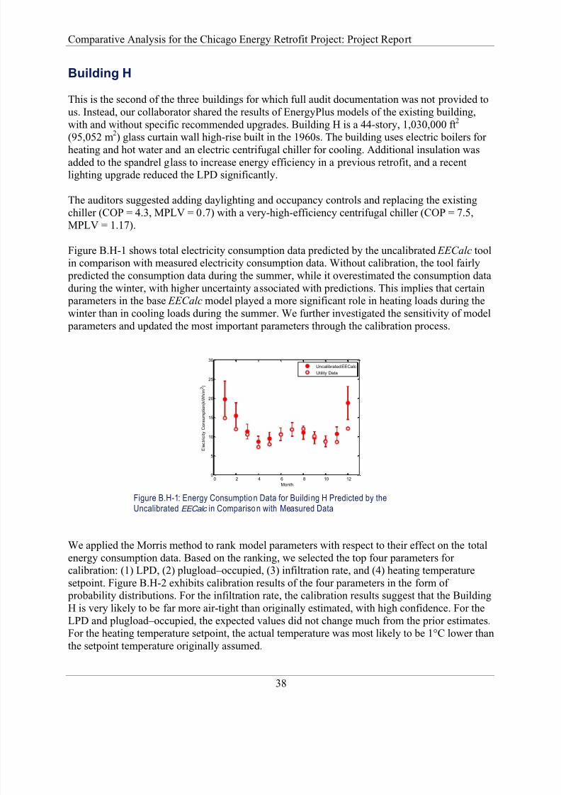
8/13/2019 ANL DIS 14.2 Chicago Loop Comparative_Analysis_FINAL.docx
http://slidepdf.com/reader/full/anl-dis-142-chicago-loop-comparativeanalysisfinaldocx 48/59
Comparative Analysis for the Chicago Energy Retrofit Project: Project Report
38
Building H
This is the second of the three buildings for which full audit documentation was not provided to
us. Instead, our collaborator shared the results of EnergyPlus models of the existing building,
with and without specific recommended upgrades. Building H is a 44-story, 1,030,000 ft2
(95,052 m2
) glass curtain wall high-rise built in the 1960s. The building uses electric boilers forheating and hot water and an electric centrifugal chiller for cooling. Additional insulation was
added to the spandrel glass to increase energy efficiency in a previous retrofit, and a recentlighting upgrade reduced the LPD significantly.
The auditors suggested adding daylighting and occupancy controls and replacing the existing
chiller (COP = 4.3, MPLV = 0.7) with a very-high-efficiency centrifugal chiller (COP = 7.5,MPLV = 1.17).
Figure B.H-1 shows total electricity consumption data predicted by the uncalibrated EECalc toolin comparison with measured electricity consumption data. Without calibration, the tool fairly
predicted the consumption data during the summer, while it overestimated the consumption dataduring the winter, with higher uncertainty associated with predictions. This implies that certain parameters in the base EECalc model played a more significant role in heating loads during the
winter than in cooling loads during the summer. We further investigated the sensitivity of model
parameters and updated the most important parameters through the calibration process.
Figure B.H-1: Energy Consumption Data for Buildi ng H Predicted by theUncalibrated EECalc in Comparison with Measured Data
We applied the Morris method to rank model parameters with respect to their effect on the total
energy consumption data. Based on the ranking, we selected the top four parameters forcalibration: (1) LPD, (2) plugload–occupied, (3) infiltration rate, and (4) heating temperature
setpoint. Figure B.H-2 exhibits calibration results of the four parameters in the form of probability distributions. For the infiltration rate, the calibration results suggest that the Building
H is very likely to be far more air-tight than originally estimated, with high confidence. For the
LPD and plugload–occupied, the expected values did not change much from the prior estimates.For the heating temperature setpoint, the actual temperature was most likely to be 1°C lower than
the setpoint temperature originally assumed.
0 2 4 6 8 10 120
5
10
15
20
25
30
Month
E l e c t r i c i t y C o n s u m p t i o n ( k W h / m 2 )
Uncalibrated EECalc
Utility Data
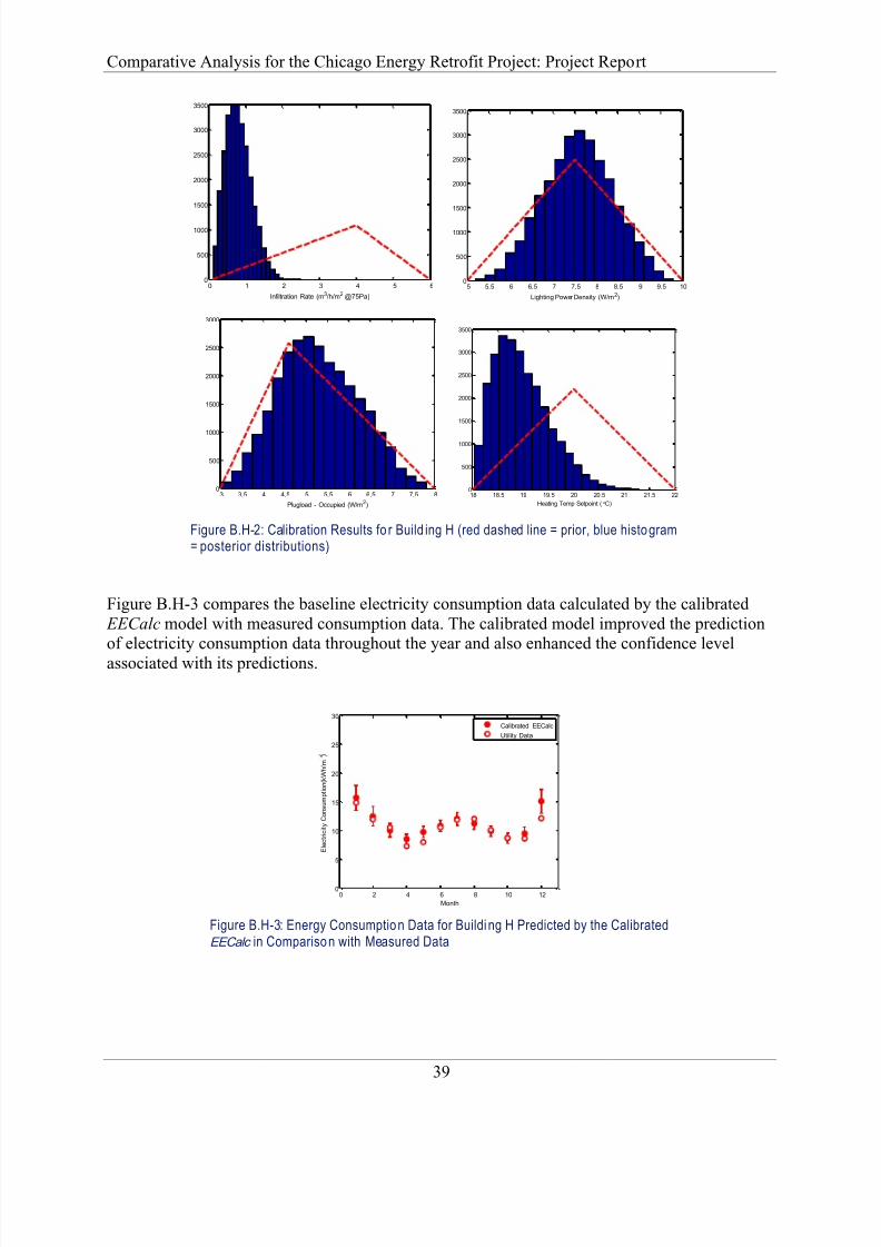
8/13/2019 ANL DIS 14.2 Chicago Loop Comparative_Analysis_FINAL.docx
http://slidepdf.com/reader/full/anl-dis-142-chicago-loop-comparativeanalysisfinaldocx 49/59
Comparative Analysis for the Chicago Energy Retrofit Project: Project Report
39
Figure B.H-2: Calibration Results fo r Build ing H (red dashed line = prior, blue histogram= posterior distributions)
Figure B.H-3 compares the baseline electricity consumption data calculated by the calibrated
EECalc model with measured consumption data. The calibrated model improved the predictionof electricity consumption data throughout the year and also enhanced the confidence level
associated with its predictions.
Figure B.H-3: Energy Consumption Data for Buildi ng H Predicted by the CalibratedEECalc in Comparison with Measured Data
0 1 2 3 4 5 60
500
1000
1500
2000
2500
3000
3500
Infiltration Rate (m3/h/m2 @75Pa)
5 5.5 6 6.5 7 7.5 8 8.5 9 9.5 100
500
1000
1500
2000
2500
3000
3500
Lighting Power Density (W/m2)
3 3.5 4 4.5 5 5.5 6 6.5 7 7.5 80
500
1000
1500
2000
2500
3000
Plugload - Occupied (W/m2)
18 18.5 19 19.5 20 20.5 21 21.5 220
500
1000
1500
2000
2500
3000
3500
Heating Temp Setpoint (C)
0 2 4 6 8 10 120
5
10
15
20
25
30
Month
E l e c t r i c i t y C o n s u m p t i o n ( k W h / m
)
Calibrated EECalc
Utility Data

8/13/2019 ANL DIS 14.2 Chicago Loop Comparative_Analysis_FINAL.docx
http://slidepdf.com/reader/full/anl-dis-142-chicago-loop-comparativeanalysisfinaldocx 50/59
Comparative Analysis for the Chicago Energy Retrofit Project: Project Report
40
We evaluated two EEMs: (1) upgrading a chiller’s efficiency from 4.3 to 7.5 and
(2) implementing lighting control (occupancy sensor and daylighting sensor). Figure B.H-4shows probability distributions of annual energy savings for each EEM. Compared with the
EECalc results, the audit project predicted higher annual energy savings for the chiller upgrade
and lower annual energy savings for the lighting upgrade.
Figure B.H-4: Probability Distributions for Building H of Annual Energy Savings from ChillerUpgrade (left) and Light ing Contro l (right). Red line is the EECalc savings prediction and theblue dashed line is the EnergyPlus saving p rediction. These results can be compared to theoverall annual use of the bu ilding which was estimated by EnergyPlus to be 133 kWh/m2.
Building I
This building is the last of three buildings for which full audit documentation was not provided
to us. Instead, our collaborator shared the results of EnergyPlus models of the existing building,
with and without specific recommended upgrades. Building I is an 18-story glass curtain wallwith 2,070,000 ft
2 (192,000 m
2) of conditioned space. It was built in the 1990s and is home to a
large data center. The data center is a ~3 MW electrical load, which includes the electrical use of
the computer room air conditioning units. This electrical load does not contribute to the buildingheating and cooling load but does contribute to the overall electrical usage of the building.
Heating and hot water are provided by electric boilers, and cooling is provided by a centrifugal
chiller. The audit evaluated a chiller upgrade and lighting upgrade with occupancy sensors and
daylighting controls.
Figure B.I-1 compares energy consumption data calculated by the uncalibrated EECalc tool with
measured data. The uncalibrated tool overestimated total electricity consumption data during the
winter, while it fairly estimated consumption data during the summer. The discrepancy betweenthe predicted and measured consumption will be reduced through calibration.
2 4 6 8 10 12 14 16 18
0
0.05
0.1
0.15
0.2
0.25
Chiller Upgrade Annual Energy Saving (kWh/m2)
P r o b a b i l i t y
88.8%
4 5 6 7 8 9 10 11 12 13 14
0
0.05
0.1
0.15
0.2
0.25
0.3
0.35
Lighting Control Annual Energy Saving (kWh/m2)
P r o b a b i l i t y
0.5%0.5%0.5%
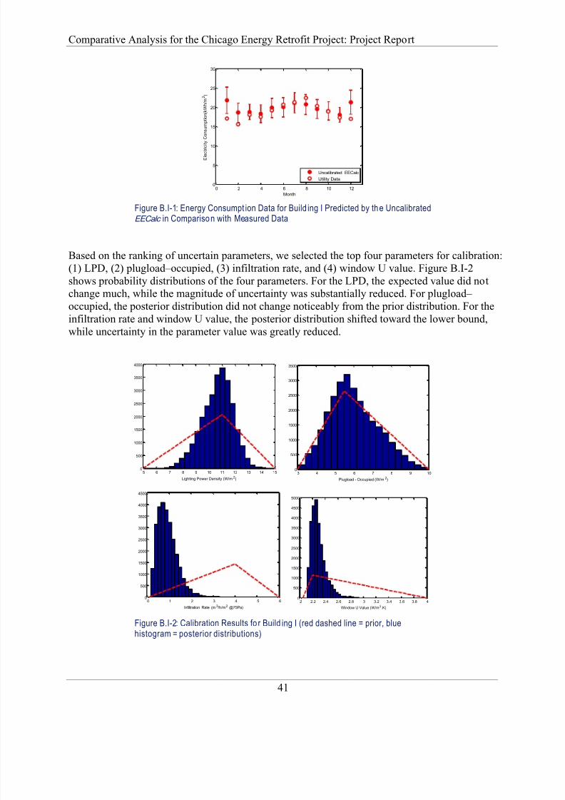
8/13/2019 ANL DIS 14.2 Chicago Loop Comparative_Analysis_FINAL.docx
http://slidepdf.com/reader/full/anl-dis-142-chicago-loop-comparativeanalysisfinaldocx 51/59
Comparative Analysis for the Chicago Energy Retrofit Project: Project Report
41
Figure B.I-1: Energy Consumpt ion Data for Build ing I Predicted by the UncalibratedEECalc in Comparison with Measured Data
Based on the ranking of uncertain parameters, we selected the top four parameters for calibration:
(1) LPD, (2) plugload–occupied, (3) infiltration rate, and (4) window U value. Figure B.I-2
shows probability distributions of the four parameters. For the LPD, the expected value did notchange much, while the magnitude of uncertainty was substantially reduced. For plugload–
occupied, the posterior distribution did not change noticeably from the prior distribution. For the
infiltration rate and window U value, the posterior distribution shifted toward the lower bound,
while uncertainty in the parameter value was greatly reduced.
Figure B.I-2: Calibration Results fo r Build ing I (red dashed line = prior, bluehistogram = posterior distributions)
0 2 4 6 8 10 120
5
10
15
20
25
30
Month
E l e c t r i c i t y C o n s u m p t i o n ( k W h / m 2 )
Uncalibrated EECalc
Utility Data
5 6 7 8 9 10 11 12 13 14 150
500
1000
1500
2000
2500
3000
3500
4000
Lighting Power Density (W/m2)
3 4 5 6 7 8 9 100
500
1000
1500
2000
2500
3000
3500
Plugload - Occupied (W/m2)
0 1 2 3 4 5 60
500
1000
1500
2000
2500
3000
3500
4000
4500
Infiltration Rate (m3/h/m2 @75Pa)
2 2.2 2.4 2.6 2.8 3 3.2 3.4 3.6 3.8 40
500
1000
1500
2000
2500
3000
3500
4000
4500
5000
Window U Value (W/m2.K)

8/13/2019 ANL DIS 14.2 Chicago Loop Comparative_Analysis_FINAL.docx
http://slidepdf.com/reader/full/anl-dis-142-chicago-loop-comparativeanalysisfinaldocx 52/59
Comparative Analysis for the Chicago Energy Retrofit Project: Project Report
42
Figure B.I-3 compares the baseline energy consumption data predicted by the calibrated EECalc
model with the measured consumption data. Although a discrepancy between predictions andmeasurements still existed, especially during the winter season, the calibration did enhance the
EECalc model so it more accurately predicted electricity consumption data in comparison with
the uncalibrated EECalc model.
Figure B.I-3: Energy Consumpt ion Data for Build ing I Predicted by the CalibratedEECalc in Comparison with Measured Data
We evaluated the two EEMs: (1) upgrading a chiller’s efficiency from 4.8 to 7.5 and
(2) implementing lighting control (occupancy sensor and daylighting control). Figure B.I-4shows probability distributions of annual energy savings against a single estimate from the audit
report per EEM. The single estimates were close to the expected values of the probabilistic
outcomes.
Figure B.I-4: Probability Distributions of Annual Energy Savings for Building I from ChillerUpgrade (left) and Ligh ting Upgrade and Contro l (right). Red line is the EECalc savingsprediction and the blue dashed line is the EnergyPlus saving pr ediction. These results canbe compared to the overall annual use of the building, which was estimated by EnergyPlus tobe 231 kWh/m2.
0 2 4 6 8 10 120
5
10
15
20
25
30
Month
E l e c t r i c i t y C o n s u m p t i o n ( k W h / m 2 )
Calibrated EECalc
Utility Data
0 2 4 6 8 10 12 14 16 180
0.02
0.04
0.06
0.08
0.1
0.12
0.14
0.16
0.18
Chiller Upgrade Annual Energy Saving (kWh/m2)
P r o b a b i l i t y
64.2%
5 10 15 20 25 30 35 40 45 500
0.01
0.02
0.03
0.04
0.05
0.06
0.07
0.08
Lighting Upgrade and Control Annual Energy Saving (kWh/m 2)
P r o b a b i l i t y
37.7%

8/13/2019 ANL DIS 14.2 Chicago Loop Comparative_Analysis_FINAL.docx
http://slidepdf.com/reader/full/anl-dis-142-chicago-loop-comparativeanalysisfinaldocx 53/59
Comparative Analysis for the Chicago Energy Retrofit Project: Project Report
43
Building J
Through the Morris method, we selected the top four important parameters with respect to their
effect on energy consumption data: (1) LPD, (2) plugload–occupied, (3) wall U value and
(4) infiltration rate. Figure B.J-1 shows probability distributions of the four parameters updated
through the calibration process. The actual LPD is very likely to be lower than our initialestimate, and uncertainty in the LPD was greatly reduced after the calibration. For the wall
U value, the expected value shifted toward the low bound by roughly 1W/m2/K. For plugload–
occupied and infiltration rate, the posterior distribution did not change much from the prior
distribution.
Figure B.J-1: Calibration Results for Bui lding J (red dashed line = prior, bluehistogram = posterior distributions)
Figure B.J-2 displays the probabilistic outcomes of gas and electricity consumption data
predicted by the calibrated EECalc model in comparison with measured data and the outcomes
predicted by the uncalibrated model. After the calibration, uncertainty in predicted energyconsumption data was greatly reduced, especially for electricity consumption predictions. The
calibrated EECalc model predicted electricity consumption more accurately than the uncalibrated
model, but the calibration did not noticeably reduce the discrepancy between predicted andmeasured gas consumption data.
10 12 14 16 18 20 22 24 26 28 300
500
1000
1500
2000
2500
3000
3500
Lighting Power Density (W/m2)
2 2.5 3 3.5 4 4.5 5 5.5 6 6.5 70
500
1000
1500
2000
2500
3000
3500
Wall U value (W/m2.K)
2 3 4 5 6 7 8 9 10 11 120
500
1000
1500
2000
2500
3000
3500
Plugload - Occupied (W/m2)
15 16 17 18 19 20 21 22 23 24 250
500
1000
1500
2000
2500
3000
3500
Infiltration Rate (m3/h/m
2 @75Pa)

8/13/2019 ANL DIS 14.2 Chicago Loop Comparative_Analysis_FINAL.docx
http://slidepdf.com/reader/full/anl-dis-142-chicago-loop-comparativeanalysisfinaldocx 54/59
Comparative Analysis for the Chicago Energy Retrofit Project: Project Report
44
Figure B.J-2: Energy Consumption Data for Building J Predicted by the Uncalibrated andCalibrated EECalc in Comparison with Measured Data
Building K Based on the ranking of model parameters by the Morris method, we selected the top four parameters for calibration: (1) plugload–occupied, (2) infiltration rate, (3) LPD, and (4) heating
temperature setpoint. Figure B.K-1 shows probability distributions of the calibration parameters
updated through the calibration process. For plugload-occupied, the calibration results reveal thatBuilding K most likely has a much higher plugload than the average plugload of office buildings.
The posterior distribution of the infiltration rate suggests that the building is likely to be much
leakier than the average building, and the magnitude of uncertainty is substantially reduced. For
the LPD, the posterior distribution did not change much from the prior distribution. For theheating temperature setpoint, the expected value shifted from 22°C to 23°C.
0 2 4 6 8 10 120
5
10
15
20
25
30
Month
G a s C o n s u m p t i o n ( k W h / m 2 )
0 2 4 6 8 10 120
2
4
6
8
10
12
14
16
18
20
Month
E l e c t r i c i t y C o n s u m p t i o n ( k W h / m 2 )
Uncalibrated EECalc
Calibrated EECalc
Utility Data

8/13/2019 ANL DIS 14.2 Chicago Loop Comparative_Analysis_FINAL.docx
http://slidepdf.com/reader/full/anl-dis-142-chicago-loop-comparativeanalysisfinaldocx 55/59
Comparative Analysis for the Chicago Energy Retrofit Project: Project Report
45
Figure B.K-1: Calibration Results for Building K (red dashed line = prior , blue histogram =posterior)
Figure B.K-2 compares the baseline electricity consumption data predicted by the calibratedmodel against measured data from the utility bills. After the calibration, the EECalc model
predicted electricity consumption data that closely matched actual consumption data. Thecomparison between the uncalibrated and calibrated model proves that calibration did not onlyenhance the model to accurately predict energy consumption data but also greatly reduced the
uncertainty in predictions.
Figure B.K-2: Energy Consumpt ion Data for Building K Predicted by theUncalibrated and Calibrated EECalc in Comparison with Measured Data
5 10 15 20 25 30 350
500
1000
1500
2000
2500
3000
3500
Plugload - Occupied (W/m2)
0 5 10 150
500
1000
1500
2000
2500
3000
3500
4000
4500
Infiltration Rate (m3/h/m2 @75Pa)
11 12 13 14 15 16 170
500
1000
1500
2000
2500
3000
Lighting Power Density (W/m2)
20 20.5 21 21.5 22 22.5 23 23.5 24 24.50
500
1000
1500
2000
2500
3000
Heating Temperature Setpoint (C)
0 2 4 6 8 10 120
5
10
15
20
25
30
35
40
45
50
Month
E l e c t r i c i t y C o n s u m p t i o n ( k W h / m
)
Uncalibrated EECalc
Calibrated EECalc
Utility Data

8/13/2019 ANL DIS 14.2 Chicago Loop Comparative_Analysis_FINAL.docx
http://slidepdf.com/reader/full/anl-dis-142-chicago-loop-comparativeanalysisfinaldocx 56/59
Comparative Analysis for the Chicago Energy Retrofit Project: Project Report
46
Building L
We applied the Morris method to identify the dominant parameters in terms of their effect on
energy consumption data. As a result, we selected the top four parameters for calibration:
(1) plugload–occupied, (2) LPD, (3) cooling system MPLV, and (4) infiltration rate.
Figure B.L-1 shows calibration results in the form of probability distributions. For plug load– occupied, the expected value is very likely to be much higher than the initial estimate, and the
magnitude of uncertainty was greatly reduced. For the LPD and cooling system MPLV, theexpected value did not change much from the prior estimates. For infiltration rate, the posterior
distribution was toward the bound, which suggests that the building envelope is very likely much
leakier than expected.
Figure B.L-1: Calibration Results for Building L (red dashed line = prior , blue histogram= posterior distribution)
Figure B.L-2 displays the probabilistic outcomes of energy consumption data predicted by thecalibrated EECalc model, the outcomes predicted by the uncalibrated model, and measured
energy consumption data. Bayesian calibration enhanced the model to represent building energy performance and significantly reduced uncertainty in baseline predictions. However, there is still
a discrepancy between predictions by the calibrated model and measurement data; the model
underpredicted total energy consumption data during the winter. This could possibly be due tounexpected changes in building operation use during the winter that were not reflected in the
model.
5 10 15 20 25 30 350
500
1000
1500
2000
2500
3000
Plugload - Occupied (W/m2)
8 10 12 14 16 18 20 22 24 260
500
1000
1500
2000
2500
3000
Lighting Power Density (W/m2)
1 2 3 4 5 6 7 8 9 100
1000
2000
3000
4000
5000
6000
Infiltration Rate (m3/h/m2 @75Pa)
0.4 0.5 0.6 0.7 0.8 0.9 1 1.1 1.2 1.30
500
1000
1500
2000
2500
3000
Cool System MPLV

8/13/2019 ANL DIS 14.2 Chicago Loop Comparative_Analysis_FINAL.docx
http://slidepdf.com/reader/full/anl-dis-142-chicago-loop-comparativeanalysisfinaldocx 57/59
Comparative Analysis for the Chicago Energy Retrofit Project: Project Report
47
Figure B.L-2: Energy Consumption Data for Building L Predicted by theUncalibrated and Calibrated EECalc in Comparison with Measured Data
Building M
After applying the Morris method, we identified the top four dominant parameters for calibration:(1) plugload–occupied, (2) LPD, (3) cooling system MPLV, and (4) infiltration rate.
Figure B.M-1 shows probability distributions of the calibration parameters. For plugload– occupied, the results suggest that actual plug load was very likely higher than the initial estimate.
For the LPD and cooling system MPLV, the expected values did not change much from the prior
estimates. For infiltration rate, the posterior distribution was toward the upper bound, whichsuggests that the building envelope was most likely much leakier than expected.
0 2 4 6 8 10 120
5
10
15
20
25
30
35
40
45
50
Month
E l e c t r i c i t y C o n s u m p t i o n ( k W h / m
)
Uncalibrated EECalc
Calibrated EECalc
Utility Data

8/13/2019 ANL DIS 14.2 Chicago Loop Comparative_Analysis_FINAL.docx
http://slidepdf.com/reader/full/anl-dis-142-chicago-loop-comparativeanalysisfinaldocx 58/59
Comparative Analysis for the Chicago Energy Retrofit Project: Project Report
48
Figure B.M-1: Calibration Results fo r Build ing M (red dashed line = prior, blue his togram =posterior distribution)
Figure B.M-2 displays the probabilistic outcomes of energy consumption data predicted by thecalibrated EECalc model in comparison with measured energy consumption data and the
outcomes predicted by the uncalibrated model. After the calibration, the EECalc accurately predicted actual electricity consumption data, with greatly reduced confidence intervals.
Figure B.M-2: Energy Consumpti on Data for Build ing M Predicted by theUncalibrated and Calibrated EECalc in Comparison with Measured Data
5 10 15 20 25 30 350
500
1000
1500
2000
2500
3000
3500
Plugload - Occupied (W/m2)
6 8 10 12 14 16 18 200
500
1000
1500
2000
2500
3000
Lighting Power Density (W/m2)
0.4 0.5 0.6 0.7 0.8 0.9 1 1.1 1.2 1.30
500
1000
1500
2000
2500
3000
Cool System MPLV
1 2 3 4 5 6 70
500
1000
1500
2000
2500
3000
3500
4000
Infiltration Rate (m3/h/m2 @75Pa)
0 2 4 6 8 10 120
5
10
15
20
25
30
35
40
45
50
Month
E l e c t r i c i t y C o n s u m p t i o n ( k W h / m
)
Uncalibrated EECalc
Calibrated EECalc
Utility Data

8/13/2019 ANL DIS 14.2 Chicago Loop Comparative_Analysis_FINAL.docx
http://slidepdf.com/reader/full/anl-dis-142-chicago-loop-comparativeanalysisfinaldocx 59/59