Anisotropic three-dimensional MHD turbulence - CORE · · 2015-06-09Anisotropic three-dimensional...

JOURNAL OF GEOPHYSICAL RESEARCH, VOL. 101, NO. A4, PAGES 7619-7629, APRIL 1, 1996

Anisotropic three-dimensional MHD turbulence

William H. Matthaeus, • Sanjoy Ghosh, D. Aaron Roberts 4

•' Se•n Oughton, s and

Abstract. Direct spectral method simulation of the three-dimensional magnetohydrodynamics (MHD) equations is used to explore anisotropy that develops from initially isotropic fluctuations as a consequence of a uniform applied magnetic field. Spectral and variance anisotropies are investigated in both compressible and incompressible MHD. The nature of the spectral anisotropy is consistent with the model of Shebalin et al. [1983] in which the spectrum broadens in the perpendicular wavenumber direction, the anisotropy being greater for smaller wavenumbers. Here this effect is seen for both incompressible and polytropic compressible MHD. In contrast, the longitudinal (compressive) velocity fluctuations remain isotropic. Variance anisotropy is observed for low plasma beta compressible MHD but not for incompressible MHD. Solar wind observations are qualitatively consistent with both variance and spectral anisotropies of the type discussed here.

Introduction

There are several motivations for investigation of dynamically appearing anisotropies in magnetohydrodynamic (MHD) turbulence: Experiments have suggested the presence of spectral anisotropy in laboratory plasma devices [e.g., Robinson and Rusbridge, 1971; Zweben et al., 1979]. Anisotropy is inherent in the "reduced" MHD description [Strauss, 1976; Montgomery and Turner, 1981; Montgomery, 1982], which never- theless must appeal to dynamical theory for its justi- fication. Variance anisotropy has also been observed by many in situ spacecraft observations [Belcher and Davis, 1971; Klein et al., 1991]. In addition, there is direct evidence of spectral anisotropy in solar wind magnetic field observations [Matthaeus et al., 1990, 1995; Bieber et al., 1995].

Important steps toward understanding MHD anisotropy were taken by Montgomery and Turner [1981] and Shebalin et al. [1983]. The former work employed perturbation theory to show that when a strong uniform magnetic field is present, the leading order fluctuations are perpendicular to it; moreover, this was shown to be consistent with measurements made in

the plasma (fusion) experiments referenced above. She- balin et al.'s simulations of two-dimensional (2D) incompressible MHD turbulence revealed development of

1 Bartol Research Institute, University of Delaware, Newark. 2 Applied Research Corporation, Landover, Maryland. 3Department of Mathematics, University College London,

London, England. 4Laboratory for Extraterrestrial Physics, Goddard Space

Flight Center, Greenbelt, Maryland.

Copyright 1996 by the American Geophysical Union.

Paper number 95JA03830. 0148-0227 / 96 / 95J A- 03830505.00

strong distinctive anisotropies in the wavenumber spectrum of the fluctuations. Recently, Oughton et al. [1994] carried out similar studies in three-dimensional (3D) incompressible MHD, applying the reasoning of She- balin et al. [1983] to describe the causes of the observed anisotropic spectral transfer. A similar kind of anisotropy can also be seen in closure calculations [Carbone and Veltri, 1990]. In the present paper we extend these investigations, asking whether compressible MHD turbulence will generate anisotropy from initially isotropic fluctuations. Furthermore, we look for the first time at the possible dynamical appearance of variance anisotropy in the simulations.

Statistical isotropy [Batchelor, 1970] is a convenient assumption in homogeneous fluid turbulence theory. Spectral density of energy is often regarded as invariant under arbitrary rotations in hydrodynamics, even with a uniform background flow (which can be eliminated by a Galilean transformation). Thus hydrodynamic anisotropies are usually connected with additional complications, such as initial data, driving effects, or inho- mogeneity. In the absence of these effects it is is possible to argue convincingly that hydrodynamics tends to become isotropic [Chandrasekhar, 1950]. However, in MHD the effects of a local mean magnetic field can- not be removed by a simple transformation to a moving frame [Elsdsser, 1956]. The mean magnetic field remains a preferred direction in any frame of reference. Consequently, anisotropy is expected when the effects of a mean magnetic field are important, as they are in MHD when the fluctuations in the magnetic field, of typical strength 5b, are not very much greater than the mean field B0.

The study of Shebalin et al. [1983] found that such anisotropy does indeed occur in MHD turbulence that begins with broadband isotropic initial data. An ap- pealing physical explanation was offered. In brief, spectral transfer occurs because of couplings among wave

7619

7620 MATTHAEUS ET AL.: ANISOTROPIC MHD TURBULENCE

vector triads; there are many of these with nonzero MHD coupling strengths. However, when a mean field is present, the condition for efficient couplings is more stringent. Resonant couplings will be the most effective, amounting to a frequency matching among the allowable triads of Fourier modes. As Shebalin et al.

noted, for resonance one member of each triad must have its wave vector perpendicular to the mean field. In a wave vocabulary this is a "nonpropagating" or "zero frequency" mode and not a linear wave eigenmode [see, e.g., Montgomery and Matthaeus, 1995]. The most efficient spectral transfer appears to be into these perpendicular Fourier modes that are not included in weak

turbulence treatments [Goldreich and Sridhar, 1995]. Consequently, anisotropic spectral transfer of this type appears to be an intrinsically nonlinear effect associated with turbulence.

Approach and Methods

Our results are obtained through direct numerical simulation of both the compressible and incompressible 3D MHD equations. The incompressible runs make use of the familiar Galerkin method [Orszag, 1971] that we have used previously, while the compressible simulations, with a polytropic equation of state, employ a pseudospectral algorithm in a familiar set of dimension- less units I Ghosh et al., 1993]. In both cases the bound- ary conditions are periodic in a cube of side 2•rL. Tak- ing the fluctuation speed as the characteristic one and L as the characteristic length, the compressible equations include an equation for continuity of mass density p,

=-v. and a momentum equation for the fluctuating velocity

Ou 1 pT j x B + u. Vu - v + + ?-1 p

where ? - 5/3 is the polytropic index and j - V x B is the electric current density, with B measured in Alfv6n speed units, i.e., let B --. B/v/4•rp0. The magnetic induction equation, in terms of the vector potential a, is

0a -u x B+pj+VF, (3)

where V x a - b, p is the resistivity, and F is the gauge function. The total magnetic field B - B0-•- b includes a uniform component, B0 - B0•, part, b. Thusj - V x b - V x B. The characteristic Mach number Ms - u/cs appears explicitly in these units and is the reciprocal of the characteristic (unit mass density) sound speed cs, measured in units of the characteristic fluctuation speed u. The viscosity v enters through the viscous dissipation term,

v_ V2 u 4- •p VV. u. (4) D,,,(u)- P

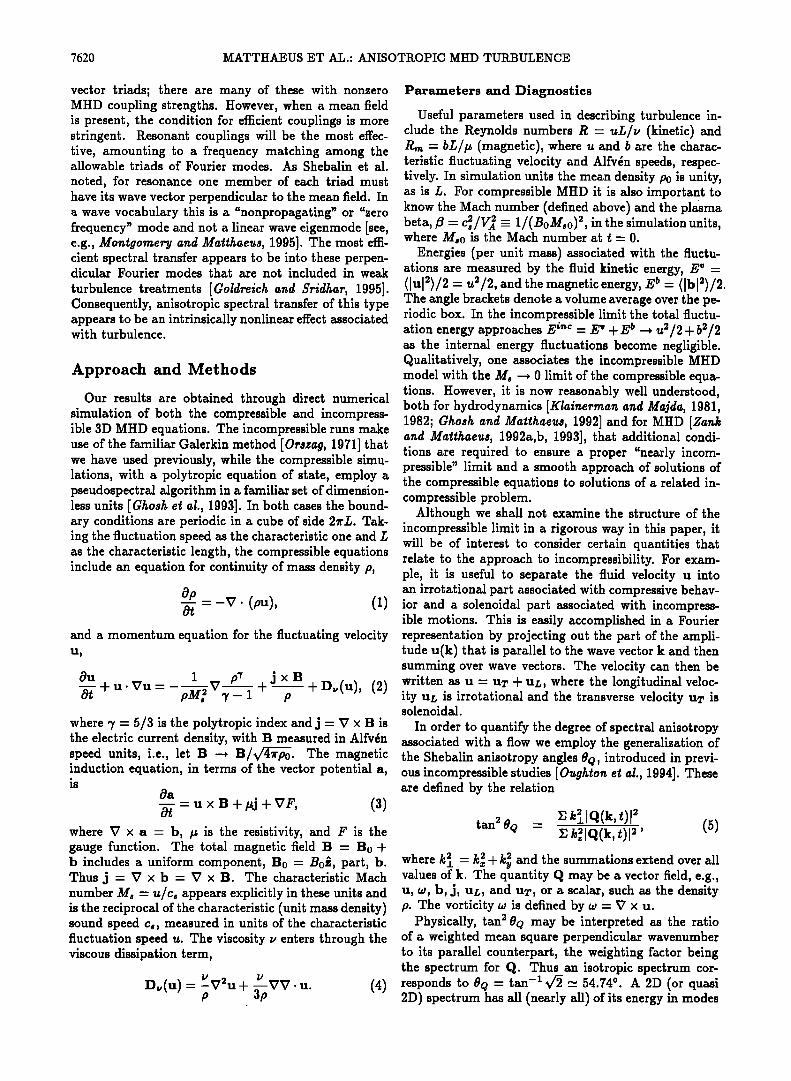
Parameters and Diagnostics

Useful parameters used in describing turbulence include the Reynolds numbers R - uL/v (kinetic) and R.m - bL/p (magnetic), where u and b are the characteristic fluctuating velocity and Alfv6n speeds, respectively. In simulation units the mean density P0 is unity, as is L. For compressible MHD it is also important to know the Mach number (defined above) and the plasma

:•/V,• - 1/(BoMso) :• in the simulation units, beta, f• -- c s , where Ms0 is the Mach number at t- 0.

Energies (per unit mass) associated with the fluctuations are measured by the fluid kinetic energy, E • = (lul-)/2 - and the magnetic energy, E The angle brackets denote a volume average over the periodic box. In the incompressible limit the total fluctuation energy approaches E inc - E • 4-E • --* u2/2 4-b2/2 as the internal energy fluctuations become negligible. Qualitatively, one associates the incompressible MHD model with the Ms -• 0 limit of the compressible equations. However, it is now reasonably well understood, both for hydrodynamics [Klainerman and Majda, 1981, 1982; Ghosh and Matthaeus, 1992] and for MHD [Zank and Matthaeus, 1992a,b, 1993], that additional conditions are required to ensure a proper "nearly incompressible" limit and a smooth approach of solutions of the compressible equations to solutions of a related incompressible problem.

Although we shall not examine the structure of the incompressible limit in a rigorous way in this paper, it will be of interest to consider certain quantities that relate to the approach to incompressibility. For example, it is useful to separate the fluid velocity u into an irrotational part associated with compressive behavior and a solenoidal part associated with incompressible motions. This is easily accomplished in a Fourier representation by projecting out the part of the amplitude u(k) that is parallel to the wave vector k and then summing over wave vectors. The velocity can then be written as u- uT-•-uL, where the longitudinal velocity uL is irrotational and the transverse velocity uT is solenoidal.

In order to quantify the degree of spectral anisotropy associated with a flow we employ the generalization of the Shebalin anisotropy angles 0Q, introduced in previous incompressible studies [Oughton et al., 1994]. These are defined by the relation

tan 20Q -- y:'/•, IQ(k, t)l (5) where k]_ - k• + k• and the summations extend over all values of k. The quantity q may be a vector field, e.g., u, w, b, j, uz,, and u7,, or a scalar, such as the density p. The vorticity w is defined by w - V x u.

Physically, tan •' 0q may be interpreted as the ratio of a weighted mean square perpendicular wavenumber to its parallel counterpart, the weighting factor being the spectrum for q. Thus an isotropic spectrum corresponds to 0q - tan -• x/• -• 54.74 ø. A 2D (or quasi 2D) spectrum has all (nearly all) of its energy in modes

MATTHAEUS ET AL.: ANISOTROPIC MHD TURBULENCE 7621

perpendicular (or nearly so) to B0 so that 8Q • 90 ø, while a slab spectrum has energy only in wave vectors along B0 and 8Q - 0.

In the present study of anisotropy the spatially uniform magnetic field B0 will always be in the •. direction so that "perpendicular" refers to the ß and y directions and "parallel" to the z direction. Spectral anisotropy will be seen to develop with respect to the B0 direction; this corresponds to an asymmetry in the distribution of scalar energy in various parts of the k space. Distinct from this is the variance anisotropy, by which we mean inequality in values of mean square components of a vector fluctuation. We designate the component variances in a s•andard way as, for example, •u2z - (u2z), etc.

Overview and Description of Runs

Our main goal is to characterize anisotropy that appears in a 3D compressible MHD model. We investigate this issue through direct numerical simulation, while also stressing comparison with similar studies of incompressible MHD [Sheba•ir• et a•., 1983; 0•ghto• •t •., 1994] (see also the 3D closure simulations of C•rbo• •r•d V•iri [1990]). Table 1 summarizes the description of the runs that will be discussed.

For a reference point we discuss a single incompressible run (c27) that is similar to those presented by 0•gh. to• •t •. [1994]. The compressible runs are se- lected to compare and contrast to the incompressible cases, as well as to explore how anisotropy may depend upon compressible MHD parameters. All the runs discussed are freely decaying initial value problems in periodic geometry and have the initial fluctuation energy E i"½ - 1 equipartitioned between the kinetic and magnetic components at all scales, i.e., E•(k)/E5(k) - 1.

All runs have equal viscosity and resistivity v - p- 1/250, so that the initial kinetic and magnetic Reynolds numbers are 250. This value is limited, as is usually the case, by the spatial resolution of the code and is chosen to give reasonably adequate resolution of the smallest dynamically important spatial scales. (Here a 643 reso-

lution is employed throughout.) The effective P•eynolds numbers decrease in time in these freely decaying turbulence simulations.

The broadband initial conditions for the runs are generated in k space. The amplitudes of u(k), for example, are chosen so that the modal kinetic energy spectrum is given by

1

E"(k) - •lu(k)l •' C

S'(k) = l+(•/•,ee)•, (6) where (7 is a normalization constant. To determine the

phase of each u(k), its real and imaginary parts are as- signed using independent Gaussian random variables. Only a subset of the retained Fourier modes are initially populated, namely those lying between two limiting values, i.e., k• _• k _• k•. The magnetic fluctuations b(k) are generated in the same fashion. The initial conditions used here all have k• - 1 and k• - 8, with kk,• -- 3 and q chosen so that the omnidirectional energy spectrum has a high-k slope of-5/3. The cross helicity (u. b) is always small.

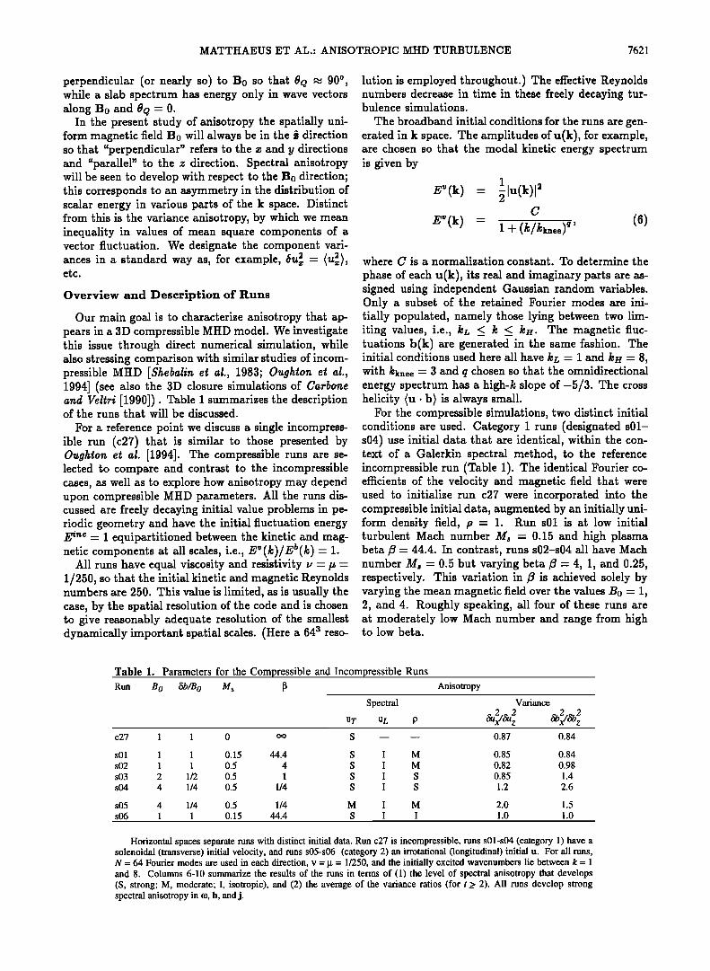
For the compressible simulations, two distinct initial conditions are used. Category 1 runs (designated s01- s04) use initial data that are identical, within the con- text of a Galerkin spectral method, to the reference incompressible run (Table 1). The identical Fourier coefficients of the velocity and magnetic field that were used to initialize run c27 were incorporated into the compressible initial data, augmented by an initially uniform density field, p - 1. P•un s01 is at low initial turbulent Mach number M, - 0.15 and high plasma beta f•- 44.4. In contrast, runs s02-s04 all have Mach number M, - 0.5 but varying beta f•- 4, 1, and 0.25, respectively. This variation in/• is achieved solely by varying the mean magnetic field over the values B0 - 1, 2, and 4. Roughly speaking, all four of these runs are at moderately low Mach number and range from high to low beta.

Table 1. Parameters for the Compressible and Incompressible Runs Run B 0 •Sb/B 0 M s [•

Spectral

UT UL P

Anisotropy

Variance

6u•/6Uz 2 2 2 c27 1 1 0 oo S -- -- 0.87 0.84

s01 1 1 0.15 44.4 S I M 0.85 0.84 s02 1 1 0.5 4 S I M 0.82 0.98 s03 2 1/2 0.5 1 S I S 0.85 1.4 s04 4 1/4 0.5 1/4 S I S 1.2 2.6

s05 4 1/4 0.5 1/4 M I M 2.0 1.5 s06 1 1 0.15 44.4 S I I 1.0 1.0

Horizontal spaces separate runs with distinct initial data. Run c27 is incompressible, runs s01-s04 (category 1) have a solenoidal (transverse) initial velocity, and runs s05-s06 (category 2) an irrotational (longitudinal) initial u. For all runs, N = 64 Fourier modes are used in each direction, v = g = 1/250, and the initially excited wavenumbers lie between k = 1 and 8. Columns 6-10 summarize the results of the runs in terms of (1) the level of spectral anisotropy that develops (S, strong; M, moderate; I, isotropic), and (2) the average of the variance ratios (for t_> 2). All runs develop strong spectral anisotropy in o0, b, and j.

7622 MATTHAEUS ET AL.' ANISOTROPIC MHD TURBULENCE

Looking at run sO1 more carefully, we note the low Mach number and isotropic initial Fourier coefficients, with uniform density and a solenoidal velocity field. Thus upon examining the appropriate criteria for ap- plicability of nearly incompressible (NI) MHD theory [Zank and Matthaeus, 1992a,b, 1993], we would con- clude that NI behavior is expected in this case and that the results should be quite similar in runs s01 and c27. Runs s02-s04 are not in the high-• regime but rather are • - (3(1) or perhaps low-• regimes. Consequently, one does not expect precise adherence to NI theory in view of the additional geometrical constraints that en- ter the theory at low • [Zank and Matthaeus, 1992a,b, 1993]. This aspect of these runs will be taken up in the discussion section.

Category 2 compressible runs (s05-s06) differ greatly from the first set, because instead of having a purely solenoidal velocity field, their Fourier coefficients have been adjusted so that u4, = 0, and thus the velocity field is purely longitudinal. This condition lies well outside the NI regime and is normally associated with acoustic or magnetoacoustic wave activity. However, the spectrum of the velocity field is the same as for the earlier runs. All runs listed in Table i use the same initial

Fourier coefficients for b.

Results

Spectral Anisotropy of Velocity and Magnetic Fields

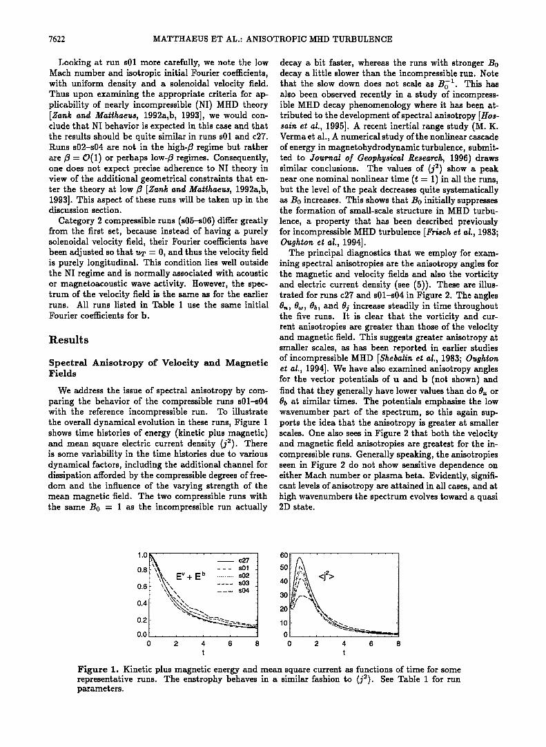
We address the issue of spectral anisotropy by com- paring the behavior of the compressible runs s01-s04 with the reference incompressible run. To illustrate the overall dynamical evolution in these runs, Figure 1 shows time histories of energy (kinetic plus magnetic) and mean square electric current density (j2). There is some variability in the time histories due to various dynamical factors, including the additional channel for dissipation afforded by the compressible degrees of freedom and the influence of the varying strength of the mean magnetic field. The two compressible runs with the same B0 = i as the incompressible run actually

decay a bit faster, whereas the runs with stronger B0 decay a little slower than the incompressible run. Note that the slow down does not scale as B• •. This has also been observed recently in a study of incompressible MHD decay phenomenology where it has been at- tributed to the development of spectral anisotropy [Hos- sain et al., 1995]. A recent inertial range study (M. K. Verma et al., A numerical study of the nonlinear cascade of energy in magnetohydrodynamic turbulence, submit- ted to Journal of Geophysical Research, 1996) draws similar conclusions. The values of (j2) show a peak near one nominal nonlinear time (t - 1) in all the runs, but the level of the peak decreases quite systematically as B0 increases. This shows that B0 initially suppresses the formation of small-scale structure in MHD turbu-

lence, a property that has been described previously for incompressible MHD turbulence [Frisch et al., 1983; Oughton et al., 1994].

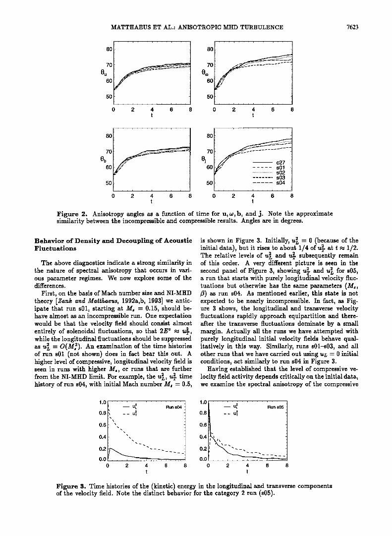
The principal diagnostics that we employ for examining spectral anisotropies are the anisotropy angles for the magnetic and velocity fields and also the vorticity and electric current density (see (5)). These are illus- trated for runs c27 and s01-s04 in Figure 2. The angles 0•, 0•, Ob, and 0j increase steadily in time throughout the five runs. It is clear that the vorticity and current anisotropies are greater than those of the velocity and magnetic field. This suggests greater anisotropy at smaller scales, as has been reported in earlier studies of incompressible MHD [Shebalin et al., 1983; Oughton et al., 1994]. We have also examined anisotropy angles for the vector potentials of u and b (not shown) and find that they generally have lower values than do 0, or Ob at similar times. The potentials emphasize the low wavenumber part of the spectrum, so this again sup- ports the idea that the anisotropy is greater at smaller scales. One also sees in Figure 2 that both the velocity and magnetic field anisotropies are greatest for the incompressible runs. Generally speaking, the anisotropies seen in Figure 2 do not show sensitive dependence on either Mach number or plasma beta. Evidently, significant levels of anisotropy are attained in all cases, and at high wavenumbers the spectrum evolves toward a quasi 2D state.

1.0

0.8

0.6

0.4

0.2

0.0

0

,.•, . - - c27 x• . . . s01

•\x. E v + E b ......... s02 '•x ..... s03 "x.•\\ .... s04 '%,

2 4 6 8

t

.at -•\

0 2 4 6 8

t

Figure 1. Kinetic plus magnetic energy and mean square current as functions of time for some representative runs. The enstrophy behaves in a similar fashion to {ja). See Table 1 for run parameters.


8O

7O

5O

2 4 6 t

80

70

50 , , , I , , , i , , , i , , ,

2 4 6 t

8O

7O

5O

8O

7O

6O

5O

0 2 4 6 8 0 t

.............. s02 s03 s04

, , , i , , , i , ß . i . . ,

2 4 6 8 t

Figure 2. Anisotropy angles as a function of time for u, w, b, and j. Note the approximate similarity between the incompressible and compressible results. Angles are in degrees.

Behavior of Density and Decoupling of Acoustic Fluctuations

The above diagnostics indicate a strong similarity in the nature of spectral anisotropy that occurs in various parameter regimes. We now explore some of the differences.

First, on the basis of Mach number size and NI-MHD theory [Zank and Matthae•s, 1992a,b, 1993] we antic- ipate that run s01, starting at M, - 0.15, should behave almost as an incompressible run. One expectation would be that the velocity field should consist almost entirely of solenoidal fluctuations, so that 2E while the longitudinal fluctuations should be suppressed

- An xminion of run s01 (not shown) does in fact bear this out. A higher level of compressive, longitudinal velocity field is seen in runs with higher M,, or runs that are further from the NI-MHD limit. For example, the u•, u•, time history of run s04, with initial Mach number M, - 0.5,

is shown in Figure 3. Initially, u• - 0 (because of the

The relative levels of u• and u• subsequently remain of this order. A very different picture is seen in the second panel of Figure 3, showing u• and u• for s05, a run that starts with purely longitudinal velocity fluctuations but otherwise has the same parameters (Ms, ]•) as run s04. As mentioned earlier, this state is not expected to be nearly incompressible. In fact, as Fig- ure 3 shows, the longitudinal and transverse velocity fluctuations rapidly approach equipartition and there- after the transverse fluctuations dominate by a small margin. Actually all the runs we have attempted with purely longitudinal initial velocity fields behave qualitatively in this way. Similarly, runs s01-s03, and all other runs that we have carried out using uL - 0 initial conditions, act similarly to run s04 in Figure 3.

Having established that the level of compressire velocity field activity depends critically on the initial data, we examine the spectral anisotropy of the compressire

1.0

0.8

0.6

0.4

0.2

0.0

0

UL Run s04

.... 2 4 6 8

t

.0 ' ' UL 2 Run s05

.6

.2 x _, ..x,,,•.•••_• _ _ .. _ _ _ _ _ _ 0 2 4 6 8

t

Figure 3. Time histories of the (kinetic) energy in the longitudinal and transverse components of the velocity field. Note the distinct behavior for the category 2 run (s05).


8O

ß 70

•- 60

5O

p Run s02

..- .

ß

8O

• 70

• 6o

50

Run s04

2 4 6 8 0 2 4 t t

i• = 1/4 -

6 8

8O

ß 70

•- 60

5O

Run s06

2 4 6 8 t

8O

• 70

• 6o

50

........... R'un 's0'5 '

,

0 2 4 6 8 t

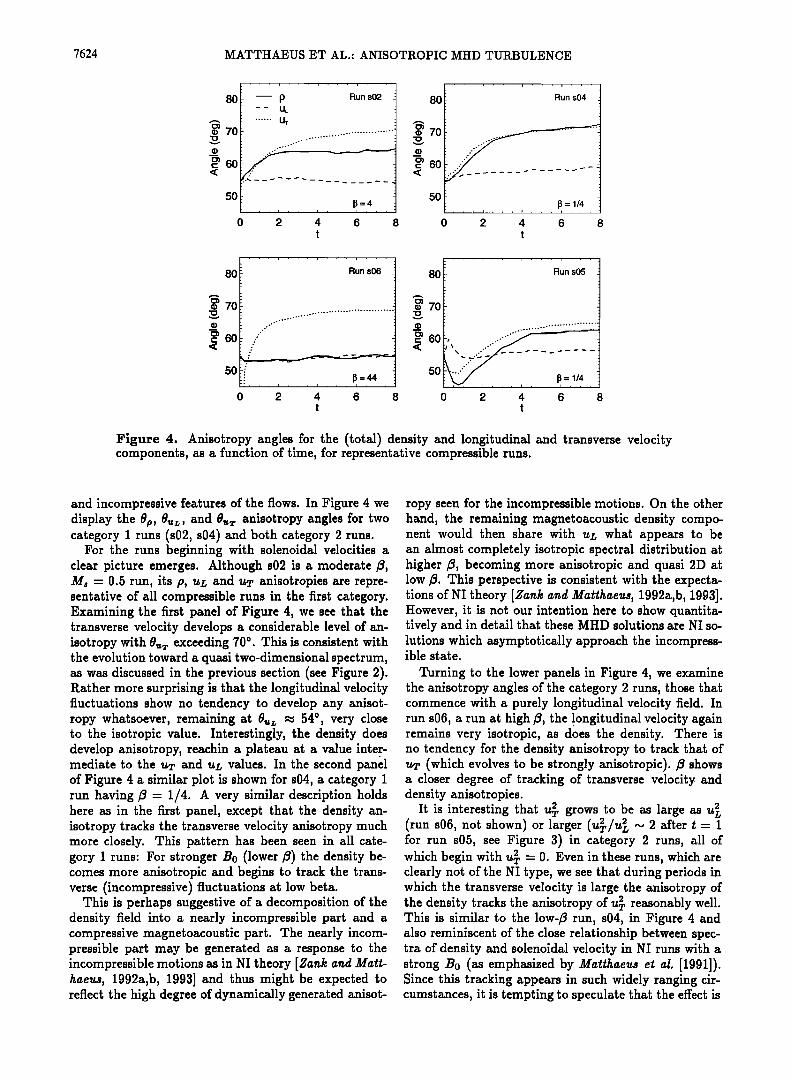
Figure 4. Anisotropy angles for the (total) density and longitudinal and transverse velocity components, as a function of time, for representative compressible runs.

and incompressive features of the flows. In Figure 4 we display the 0p, 0,•, and •-T anisotropy angles for two category i runs (s02, s04) and both category 2 runs.

For the runs beginning with solenoidal velocities a clear picture emerges. Although s02 is a moderate M• = 0.5 run, its p, uL and u•r anisotropies are representative of all compressible runs in the first category. Examining the first panel of Figure 4, we see that the transverse velocity develops a considerable level of anisotropy with •,T exceeding 70 ø. This is consistent with the evolution toward a quasi two-dimensional spectrum, as was discussed in the previous section (see Figure 2). Rather more surprising is that the longitudinal velocity fluctuations show no tendency to develop any anisotropy whatsoever, remaining at •,• m 54 ø, very close to the isotropic value. Interestingly, the density does develop anisotropy, reachin a plateau at a value intermediate to the u•r and uL values. In the second panel of Figure 4 a similar plot is shown for s04, a category 1 run having •3 = 1/4. A very similar description holds here as in the first panel, except that the density anisotropy tracks the transverse velocity anisotropy much more closely. This pattern has been seen in all category 1 runs: For stronger B0 (lower •3) the density becomes more anisotropic and begins to track the transverse (incompressive) fluctuations at low beta.

This is perhaps suggestive of a decomposition of the density field into a nearly incompressible part and a compressive magnetoacoustic part. The nearly incompressible part may be generated as a response to the incompressible motions as in NI theory [Zank and Matt- haeus, 1992a,b, 1993] and thus might be expected to reflect the high degree of dynamically generated anisot-

ropy seen for the incompressible motions. On the other hand, the remaining magnetoacoustic density component would then share with u• what appears to be an almost completely isotropic spectral distribution at higher •3, becoming more anisotropic and quasi 2D at low •3. This perspective is consistent with the expecta- tions of NI theory [Zank and Matthaeus, 1992a,b, 1993]. However, it is not our intention here to show quantitatively and in detail that these MHD solutions are NI solutions which asymptotically approach the incompressible state.

Turning to the lower panels in Figure 4, we examine the anisotropy angles of the category 2 runs, those that commence with a purely longitudinal velocity field. In run s0õ, a run at high •3, the longitudinal velocity again remains very isotropic, as does the density. There is no tendency for the density anisotropy to track that of wr (which evolves to be strongly anisotropic). f• shows a closer degree of tracking of transverse velocity and density anisotropies.

It is interesting that u} grows to be as large as u} (run s06, not shown) or larger (u.•lu} ~ 2 after t- 1 for run s05, see Figure 3) in category 2 runs, all of which begin with u•. - 0. Even in these runs, which are clearly not of the NI type, we see that during periods in which the transverse velocity is large the anisotropy of the density tracks the anisotropy of u•, reasonably well. This is similar to the low-• run, s04, in Figure 4 and also reminiscent of the close relationship between spectra of density and solenoidal velocity in NI runs with a strong Bo (as emphasized by Matthaeus et at. [1991]). Since this tracking appears in such widely ranging cir- cumstances, it is tempting to speculate that the effect is


robust and that even a small increase in uT over uL may be enough to trigger a clear and observable relationship between density and solenoidal velocity spectra.

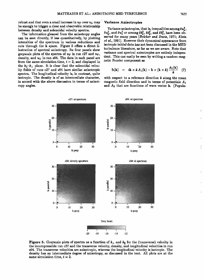
The information gleaned from the anisotropy angles can be seen directly, if less quantitatively, by plotting intensities of the spectrum in various reductions and cuts through the k space. Figure 5 offers a direct il- lustration of spectral anisotropy. Its four panels show greyscale plots of the spectra of ul, in run c27 and ul,, density, and uz, in run s04. The data in each panel are from the same simulation time, t - 2, and displayed in the kll-k_• plane. It is clear that the solenoidal velocity fields of runs c27 and s04 have similar anisotropic spectra. The longitudinal velocity is, in contrast, quite isotropic. The density is of an intermediate character, in accord with the above discussion in terms of anisot-

ropy angles.

Variance Anisotropies

Variance anisotropies, that is, inequalities among 5u•, and 5u,• or among 5b•, 5b•, and 5b, •, have been observed for many years [Belcher and Davis, 1971; Klein et al., 1991]. However their dynamical appearance from isotropic initial data has not been discussed in the MHD turbulence literature, as far as we are aware. Note that variance and spectral anisotropies are entirely independent. This can easily be seen by writing a random magnetic Fourier component as

•(•) - i• x i •(•)- • x (• x •) •'(•) • (7) with respect to a reference direction • along the mean magnetic field direction and in terms of potentials A x and A2 that are functions of wave vector k. (Popula-

3O

c27: ut spectrum ..

3O

s04: ut spectrum

..

.

.;i;½;};•ji•,;,..,,,;•i...=.:, = 'q•_.,•2' ' • '"'•::•:• 0

0 10 20 30 0 10 20 30

k-perp k-perp

s04: density spectrum

20

-• 10 •.•ii•,•...'• ..............

0 10 20

k-pe•

3O

2O

s04: ul spectrum

•..',,•' :..:,•,/• ....... ,.. •.:•....:...-..•,.: ....................... -. :..- ..... :30

•!,"

0 10 20

k-pe•

3O

Grey Scale

-20 -18 -16 -14 -12

Figure 5. Greyscale plots of spectra as a function of kz and kll for the (transverse) velocity in the incompressible run c27 and the transverse velocity, density, and longitudinal velocities in run s04. The transverse velocities are anisotropic, whereas the longitudinal velocity is isotropic. The density has an intermediate degree of anisotropy, as discussed in the text. All plots are at the same simulation time, t - 2.


tion of "slab" wave vectors along •. must be handled separately or by a limiting procedure.) It is clear that one can render the fluctuations entirely transverse to the mean field by setting A2 - 0 for all k. Thus variance anisotropy is controlled by the relative size of A• and A2, whereas spectral anisotropy is a consequence of the way that the potentials depend upon the direction of k. "Minimum variance arguments" are sometimes used to link variance and spectral anisotropies. While this is a useful method, it is inappropriate to deduce that energetically populated wave vectors must lie in the minimum variance direction. As a counterexample, consider the case of 2D turbulence with A2 - 0 and A x - A x (k•, k•), independent of z. Then, 5u• - 0 and the minimum variance direction is along z. However, all populated wave vectors are in the z,y plane.

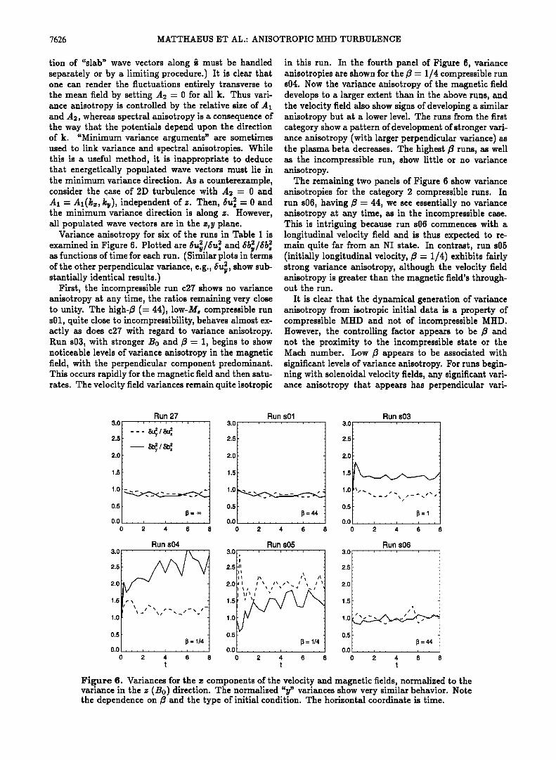
Variance anisotropy for six of the runs in Table 1 is examined in Figure 6. Plotted are • • • 2 5t%/Stt• and 5b•/Sb• as functions of time for each run. (Similar plots in terms of the other perpendicular variance, e.g., &t•, show sub- stantially identical results.)

First, the incompressible run c27 shows no variance anisotropy at any time, the ratios remaining very close to unity. The high-/S (= 44), low-M, compressible run s01, quite close to incompressibility, behaves almost ex- actly as does c27 with regard to variance anisotropy. Run s03, with stronger B0 and/S - 1, begins to show noticeable levels of variance anisotropy in the magnetic field, with the perpendicular component predominant. This occurs rapidly for the magnetic field and then satu- rates. The velocity field variances remain quite isotropic

in this run. In the fourth panel of Figure 6, variance anisotropies are shown for the/S = 1/4 compressible run s04. Now the variance anisotropy of the magnetic field develops to a larger extent than in the above runs, and the velocity field also show signs of developing a similar anisotropy but at a lower level. The runs from the first category show a pattern of development of stronger variance anisotropy (with larger perpendicular variance) as the plasma beta decreases. The highest/S runs, as well as the incompressible run, show little or no variance anisotropy.

The remaining two panels of Figure õ show variance anisotropies for the category 2 compressible runs. In run sO6, having/S - 44, we see essentially no variance anisotropy at any time, as in the incompressible case. This is intriguing because run s0õ commences with a longitudinal velocity field and is thus expected to remain quite far from an NI state. In contrast, run s05 (initially longitudinal velocity,/S = 1/4) exhibits fairly strong variance anisotropy, although the velocity field anisotropy is greater than the magnetic field's throughout the run.

It is clear that the dynamical generation of variance anisotropy from isotropic initial data is a property of compressible MHD and not of incompressible MHD. However, the controlling factor appears to be /S and not the proximity to the incompressible state or the Mach number. Low /S appears to be associated with significant levels of variance anisotropy. For runs beginning with solenoidal velocity fields, any significant variance anisotropy that appears has perpendicular vari-

3.0

2.5

2.0

1.5

1.0

0.5

Run 27 ' ' ' , ' ' ' • ß . . i . . .

_ _. •,/

0.0 ...............

0 2 4 6 8

Run s01 , , , [ , , , • , , , , , , ,

I• =44

0 2 4 6 8

Run s03 ' ß m . , . i , , ,

0 2 4 6 8

Run s04

1.5

1.0

0.5

I• = 1/4

0 2 4 6 8 t

Run s05 , , , [ , , , ! , , , , , , ,

; -I! .

• = 1/4

0 2 4 6 8 t

Run s06 ' ' ' m , , , i ' ' ' i , , ,

=44

8

Figure 6. Variances for the a• components of the velocity and magnetic fields, normalized to the variance in the z (B0) direction. The normalized "y" variances show very similar behavior. Note the dependence on/S and the type of initial condition. The horizontal coordinate is time.


ances larger than the parallel one. The nature of low-• variance anisotropy can be different in the highly com- presslye category 2 runs, in which larger parallel variance sometimes occurs, and more importantly, the variance anisotropy of the velocity is larger than that of the magnetic field.

Summary and Discussion

In this paper we have examined the nature of spectral and variance anisotropies in three-dimensional compressible and incompressible MHD turbulence for periodic geometry. The incompressible case has been exten- sively studied previously [Shebalin et al., 1983; Carbone and Veltri, 1990; Oughton et al., 1994]. We have seen that in the compressible runs, spectral anisotropy dynamically develops in much the same way as has been reported for incompressible MHD. The anisotropy angles associated with the velocity, magnetic, vorticity, and electric current density fields generally increase in time. These angles indicate the angular separation of typical excitations from the mean magnetic field axis. As these angles approach 900 , the spectrum becomes concentrated in the 2D plane perpendicular to the mean magnetic field, suggesting a quasi 2D state. For the cases we examined the velocity and magnetic field anisotropy angle had values comparable to a similar incompressible run. Also, as in the incompressible case, greater anisotropy is indicated at smaller scales. This strong similarity to the incompressible behavior suggests that the mechanism for dynamical production of spectral anisotropy in incompressible MHD [Shebalin et al., 1983] is also important for compressible MHD turbulence.

A more complex picture emerges when we examine the spectral anisotropy of the density and the longitudinal ("L)and transverse ("T)parts of the velocity field. The longitudinal velocity, representative of purely compressive fluctuations, remains almost completely isotropic throughout all runs with all values of /•, B0, and Ms that we have investigated, including runs commencing with either purely uL or purely u• fluctuations. Also, in all cases, u• (ordinarily associated in a direct way with incompressive motions) always appears to evolve toward an anisotropic state of the quasi 2D type. In contrast, the behavior of the density varies con- siderably. On the basis of category 1 runs it is tempting to say that the density follows tendencies that can be understood in terms of nearly incompressible theory [Za•k a•d Matthaeus, 1992a,b, 1993]. Indeed, for category 1 runs (at least some of which may be truly NI runs) this description seems to work well. However, this reasoning would not apply in any obvious way to category 2 runs, which initially have only compressive, longitudinal fluctuations. Such runs are far from NI. It appears that the transverse velocity tends toward quasi 2D spectral distributions when in the NI limit and also somewhat beyond any regime in which near- incompressibility is quantitatively defensible. The spectral anisotropy of the density seems to vary somewhat

but generally lies between the values for ug (isotropic) and u• (quasi 2D). The factors that control where the density anisotropy falls between these (approximate) limits appear to be the plasma f• and the proximity to an incompressible state (i.e., u•. ) uL). Low f• favors a density anisotropy that tracks that of u.r. Further investigation of this complicated behavior of the spectral anisotropy of the density appears to be needed before a full explanation can be claimed.

Compressible MHD turbulence is quite different from its incompressible counterpart with regard to the appearance of variance anisotropy. For incompressible turbulence, no significant level of variance anisotropy appears in the simulations we have examined. However, in the compressible case a systematic pattern appears in which greater variance anisotropy is associated with lower plasma/•. For simulations with initially solenoidal velocity fields (category 1 runs) the variance anisotropy of the magnetic field is generally greater than that of the velocity field. Furthermore, for both u and b the perpendicular components of the variance exceed the parallel ones. For simulations that begin with a purely longitudinal velocity field (category 2), variance anisotropies also tend to appear at low f•, but now the velocity variance anisotropy is greater than that of the magnetic field.

Connections of the present study to solar wind observations are clearly indicated. First, there is a body of accumulated prior evidence that spectral anisotropy is expected in a turbulent magnetofluid such as the solar wind [e.g., Matthaeus et al., 1995]. Direct observations suggest that solar wind fluctuations are anisotropic [Carbone et al., 1995] and contain a significant admix- ture of 2D or quasi 2D spectral symmetry [Matthaeus et al., 1990; Bieber et al., 1995]. In the above results we see for the first time the suggestion in turbulence simulations that the solar wind variance anisotropy might be explained by in situ compressible turbulence. So- lar wind variance inequality was originally discussed by Belcher and Davis [1971], who quote a 5:4:1 ratio of magnetic variances, the smallest being the parallel direction. More recently, Klein et al. [1991] examined both velocity and magnetic field variances, from 1- and 3-hour samples of Voyager data ranging from i AU to beyond 10 AU. Their results indicate variance anisotropies in both fields, with larger perpendicular component variances and larger anisotropy for the magnetic field. For the magnetic field the variance anisotropy lies in the range of 2 to 4 between 1 and 10 AU, while it remains about 2 for the velocity field. This is quite consistent with the pattern observed in the present category 1 simulations, except that the simulations at /• - 1/4 showed somewhat smaller values,

5u•/Su z • 1.2. Clearly, any complete discussion of the nature of spec-

tral and variance anisotropy in the solar wind would have to include many factors that are well beyond the scope of the present study. These would certainly in- volve radial expansion and the influence of large-scale shear and stream structure, which would induce pre-

7628 MATTHAEUS ET AL.: ANISOTROPIC MIlD TURBULENCE

ferred directions on the turbulence beyond only the mean magnetic field direction considered here. Further- more, the Reynolds numbers characterizing the solar wind are most likely enormously greater than our com- putational values. (There is some evidence that MHD anisotropies become greater at higher Reynolds numbers [Oughton et al., 1994].) Another ambiguity in applying the present study to the solar wind is that there are various locations in the heliosphere where dynamical anisotropy might be generated and then subsequently convected and modified. The mechanism we have de-

scribed might come into play in the lower corona, prior to acceleration of the supersonic wind, and it might also be active in the wind itself.

There are also limitations to the MHD model em-

ployed here. For example, a strong B0 significantly modifies the viscous stress tensor so that (4) is replaced by a highly anisotropic form [e.g., Braginskii, 1065]. Montgomery [1992] has suggested that this form may be appropriate for describing MHD turbulence in the solar wind and in fact may be significant at all spatial scales because of the large value of the ion parallel viscosity coefficient. In addition, since the polytropic index 3' is related to the number of degrees of freedom associated with the fluid, it should probably be a function of the effective dimensionaltry of the system rather than a fixed constant. Thus it may be that 3' is a function of the plasma/3. A full investigation of these possibilities and complications is far beyond our present goal of characterizing a potentially important basic MHD turbulence process.

However, if MHD turbulence is indeed responsible for the variance anisotropies in the solar wind, the present results suggest that the solar wind fluctuations are not highly compressire like the category 2 simulations here that started from purely longitudinal velocity fields. Al- though the mechanism for production of the variance anisotropy in the simulations is not yet entirely understood, there is some indication that it is connected with low/3. This is suggestive of the constraints that arise in nearly incompressible theory in the low-/3 limit [Zank and Matthaeus, 1992a,b, 1993]. In such cases the approach to incompressibility demands that the turbulence reside in a state of almost 2D spectral anisotropy, while also having small O(M,) parallel velocity and magnetic field components. Thus in the low-/•, low-M, NI limit the variance anisotropies become quite large. This pattern is suggestively similar to what we observe in the simulations. However, this falls far short of an explanation in view of the fact that we have not verified that these simulations, especially those at low/•, are of the proper NI variety. In particular, we have not attempted to obey the geometrical constraint of spectral anisotropy in the initial data that is required for the low-• NI limit.

We are left with a partially satisfying conclusion. Compressible simulations show that locally homogeneous MHD turbulence can produce important features of the spectral and variance anisotropies that are cur- rently thought to characterize solar wind turbulence.

These features are exhibited when the turbulence oc-

curs in the presence of a mean magnetic field, when it is not too far from incompressibility, and when the plasma • is unity or lower. The explanation of the appearance of the spectral anisotropy appears to be firm, the available explanations for the appearance of variance anisotropies, based upon nearly incompressible theory, is an incomplete subject. It is likely that future studies will serve to further clarify various issues regarding anisotropies that appear in MHD, including theoretical refinements and additional observational connections.

Acknowledgments. This research has been supported in part by NASA through the Space Physics Theory Pro- grams at Goddard Space Flight Center and at Bartol and by the NSF through grant ATM-9318728 at Bartol. Com- putational resources have been provided by the San Diego Supercomputing Center and by the NCCS at GSFC.

The Editor thanks J. W. Freeman and another referee for

their assistance in evaluating this paper.

References

Batchelor, G. K., The Theory oy Homogeneous Turbulence, Cambridge Univ. Press, New York, 1970.

Belcher, J. W., and L. Davis Jr, Large-amplitude Alfv•n waves in the interplanetary medium, 2, J. Geophys. Res., 76, 3534, 1971.

Bieber, J. W., W. Wannet, and W. H. Matthaeus, Dominant two-dimensional solar wind turbulence with implications for cosmic ray transport, Y. Geophys. Res., in press, 1995.

Braginskii, S. I., Transport processes in a plasma, Rev. Plasma Phys., 1, 205, 1965.

Carbone, V., and P. Veltri, A shell model for anisotropic magnetohydrodynamic turbulence, Geophys. Astrophys. Fluid Dyn., 52, 153, 1990.

Carbone, V., F. Malara, and P. Veltri, A model for the three-dimensional magnetic field correlation spectra of low-frequency solar wind fluctuations during Alfv•nic periods J. Geophys. Res., 100, 1763, 1995.

Chandrasekhar, S., The theory of axisymmetric turbulence, Philos. Trans. Roy. Soc. London Set. A, 2•2, 557, 1950.

Els/isser, W. M., Ilydromagnetism, II, A review, Am. J. Phys., 2•, 85, 1956.

Frisch, U., A. Pouquet, P.-L. Sulem, and M. Meneguzzi, The dynamics of two-dimensional ideal MILD, J. Mdc. Thdor. Appl., 216, 191, 1983.

Ghosh, S., and W. If. Matthaeus, Low Mach number two- dimensional hydrodynamic turbulence: Energy budgets and density fluctuations in a polytropic fluid, Phys. Flu- ids A, •, 148, 1992.

Ghosh, S., M. flosssin, and W. If. Matthaeus, The applica- tion of spectral methods in simulating compressible fluid and magnetofluid turbulence, Cornput. Phys. Cornrnun., ?•, 18, 1993.

Goldreich, P., and S. Sridhar, Toward a theory of interstellar turbulence, II, Strong Alfv•nic turbulence, Astrophys. J., •38, 763, 1995.

flosssin, M., P. C. Gray, D. If. Pontius, Jr., W. If. Matt- haeus, and S. Oughton, Phenomenology for the decay of energy-containing eddies in homogeneous MHD turbulence, Phys. Fluids, 7, 2886, 1995.

Klainerman, S., and A. Maids, Singular limits of quasilln- ear hyperbolic systems with large parameters and the incompressible limit of compressible fluids, Cornrnun. Pure Appl. Math., 3•, 481, 1981.


Klainerman, S., and A. Majda, Compressible and incompressible fluids, Cornrnun. Pure Appl. Math., 35, 629, 1982.

Klein, L. W., D. A. Roberts, and M. L. Goldstein, Anisot- ropy and minimum variance directions of solar wind fluctuations in the outer heliosphere, J. Geophys. Res., 96, 3779, 1991.

Matthaeus, J. V. S. W. H., and D. Montgomery, Anisot- ropy in MHD turbulence due to a mean magnetic field, J. Plasma Phys., $9, 525, 1983.

Matthaeus, W. H., M. L. Goldstein, and D. A. Roberts, Evidence for the presence of quasi two-dimensional nearly incompressible fluctuations in the solar wind, J. Geophys. Res., 95, 20, 1990.

Matthaeus, W. H., L. W. Klein, S. Ghosh, and M. R. Brown, Nearly incompressible magnetohydrodynamics, pseudo- sound, and solar wind fluctuations, J. Geophys. Res., 96, 5421, 1991.

Matthaeus, W. H., J. W. Bieber, and G. P. Zank, Unquiet on any front: Anisotropic turbulence in the solar wind, U.S. Natl. Rep. Int. Union Geod. Geophys. 1991-199g, Rev. Geophyz., 33, 609, 1995.

Montgomery, D.C., Major disruption, inverse cascades, and the Strauss equations, Phyz. Scr., TI/$, 83, 1982.

Montgomery, D.C., Modifications of magnetohydrodynamics as applied to the solar wind, J. Geophys. Res., 97, 4309, 1992.

Montgomery, D.C., and W. H. Matthaeus, Anisotropic modal energy transfer in interstellar turbulence, Astro- phys. J., •47, 706, 1995.

Montgomery, D.C., and L. Turner, Anisotropic magnetohydrodynamic turbulence in a strong external magnetic field, Ph!ls. Fluids, $j, 825, 1981.

Orszag, S. A., Numerical simulation of incompressible flows within simple boundaries: I. Galerkin (spectral) represen- tations, Stud. Appl. Math., 50, 293, 1971.

Oughton, S., E. R. Priest, and W. H. Matthaeus, The influence of a mean magnetic field on three-dimensional MHD turbulence, J. Fluid Mech., $80, 95, 1994.

Robinson, D., and M. Rusbridge, Structure of turbulence in the zeta plasma, Phys. Fluids, lj, 2499, 1971.

Strauss, H. R., Nonlinear, three-dimensional magnetohydrodynamics of noncircular tokamaks, Phys. Fluids, 19, 134, 1976.

Zank, G. P., and W. H. Matthaeus, The equations of reduced magnetohydrodynamics, J. Plasma Phys., gS, 85, 1992a.

Zank, G. P., and W. H. Matthaeus, Waves and turbulence in the solar wind, J. Geophys. Res., 97, 17, 1992b.

Zank, G. P., and W. H. Matthaeus, Nearly incompressible fluids, II, Magnetohydrodynamics, turbulence, and waves, Phys. Fluids A, 5, 257, 1993.

Zweben, S., C. Menyuk, and R. Taylor, Small-scale magnetic fluctuations inside the macrotor tokamak, Phys. Rev. Left., g$, 1270, 1979.

S. Ghosh, Applied Research Corporation, 8201 Corpo- rate Drive Suite 1120, Landover, MD 20785.(e-maih r on. ghosh • gsfc. nasa. gov)

W. H. Matthaeus, Bartol Research Institute, Uni- versity of Delaware, Newark, DE 19716. (e-maih yswhm•bartol.udel.edu)

S. Oughton, Department of Mathematics, University Col- lege London, London, WCIE 6BT, England. (e-mail: sean •ma t h. u cl.ac. uk)

D. A. Roberts, Laboratory for Extraterrestrial Physics, Goddard Space Flight Center, Greenbelt, MD 20771. (e-maih Dana. A. Roberts. [email protected])

(Received October 2, 1995; revised December 13, 1995; accepted December 19, 1995.)

Anisotropic three-dimensional MHD turbulence - CORE · · 2015-06-09Anisotropic three-dimensional...

Documents

Transcript of Anisotropic three-dimensional MHD turbulence - CORE · · 2015-06-09Anisotropic three-dimensional...