ANIMATED STUDY SIMULATION OF ALTERNATIVES FOR TOW …
103
ANIMATED STUDY SIMULATION OF ALTERNATIVES FOR TOW LAUNCH PRODUCTION AT THE RADFORD ARMY AMMUNITION PLANT BV Project submitted to the Faculty of Virginia Polytechnic Institute and State University In panlal fuHlllment 01 the requirements for the degree of Master of Eng Ineerlng In Industrial And Systems Engineering APPROVED: R. J. Reasor (Chairman) Fab""IY.1 .. a
Transcript of ANIMATED STUDY SIMULATION OF ALTERNATIVES FOR TOW …

ANIMATED STUDY SIMULATION OF ALTERNATIVES
FOR TOW LAUNCH PRODUCTION
AT THE RADFORD ARMY AMMUNITION PLANT
BV
Project submitted to the Faculty of Virginia Polytechnic Institute and State University In panlal fuHlllment 01 the requirements for the
degree of
Master of Eng Ineerlng In
Industrial And Systems Engineering
APPROVED:
R. J. Reasor (Chairman)
Fab""IY.1 .. a

LD t::~~ C"l:-" ~CR"";":';
i.J&SI J1~?;S
L 71-/6
ABSTRACT
ANIMATED SIMULATION TO STUDY MATERIAL HANDLING SYSTEMS FOR
TOW LAUNCH PRODUCTION AT THE RADFORD ARMY AMMUNITION PLANT
By
DIIn A. ereme,
CommIttee e .......... n: R .... Re.so,
The objective of this project Is to Investigate the present process required to
manufacture the TOW Launch propellant and anticipate the resources required to
manufacture a reduced amount of demand. This will be done using animated simulation
techniques.
The Radford Army AmmunHlon Plant was designed for extremely high volumes of
propellant manufacturing. Due to the recent cut backs In defense spending, the demands
for such high volumes no longer exlSlS. However, the plant continues to operate In a high
volume mode. A method to determine the resources which can be eliminated as production
Is scaled down, and stili not be delinquent on any orders, Is required. Ttlls method would
help define the resource capacHIes under the present mode of operation.

Acknowledgement
The undertaking and completion of this project would not have been possible without
the careful guidance from Professor R. J. Reasor, Industrial and Systems Engineering at
Virginia Polytechnic Institute and State University, to whom I express my sincere
appreciation. Funher acknowledgement Is extended to Dr. J. D. Tew and Dr. W. J. Fabrycky
for serving on my advisory committee.
My deepest appreciation extends to my wife and children who had to make sacrifices
while I completed this degree.
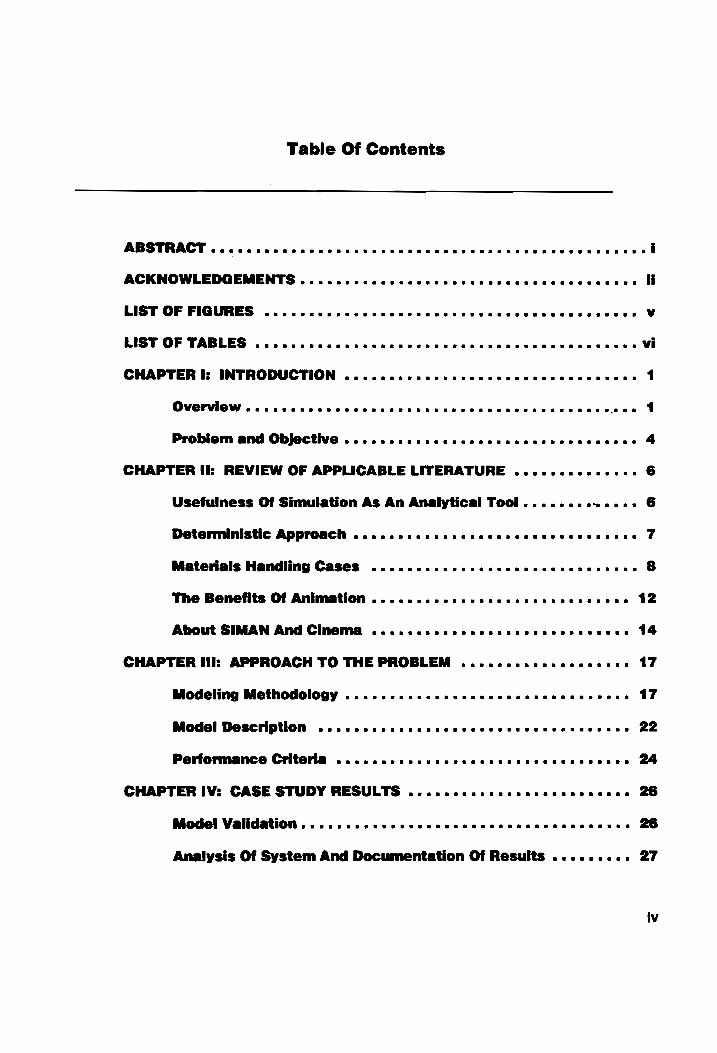
Table Of Contents
ABSTRACT ••••••••••••••••••••••••••••••••••••••••••••••••• I
ACKNOWLEDGEMENTS • • • • • • • • • • • • • • • • • • • • • • • • • • • • • • • • • • • • •• II
LIST OF FIGURES •••••••••••••••••••••••••••••••••••••••••• v
LIST OF TABLES ••••••••••••••••••••••••••••••••••••••••••• vi
CHAPTER I: INTRODUCTION ••••••••••••••••••••••••••••••••• 1
Overview. • • • • • • • • • • • • • • • • • • • • • • • • • • • • • • • • • • • • • • • •.• •• 1
Probl.m and Objective • • • • • • • • • • • • • • • • • • • • • • • • • • • • • • • •• 4
CHAPTER II: REVIEW OF APPLICABLE LITERATURE •••••••••••••• 6
Usefulness Of Simulation As An Analytlca' Tool • • • • • • • ... • • •• 6
Detenninlstlc Appl'Ollch •••••••••••••••••••••••••••••••• 7
Materials Handling Cases •••••••••••••••••••••••••••••• 8
The Benefits Of Anlnatlon ............................. About SIMAN And Cinema •••••••••••••••••••••••••••••
CHAPTER III: APPROACH TO THE PROBLEM •••••••••••••••••••
Modeling M.thodolog, ••••••••••••••••••••••••••••••••
Model Description ...................................
12
14
17
17
22
Perlonnance Crlt..... ••••••••••••••••••••••••••••••••• 24
CHAPTER IV: CASE STUDY RESULTS ••••••••••••••••••••••••• 26
Model Vall.tion • • • • • • • • • • • • • • • • • • • • • • • • • • • • • • • • • • • •• 28
Anal,sls Of System And Documentation Of Results ••• • • • • •• 27
Iv
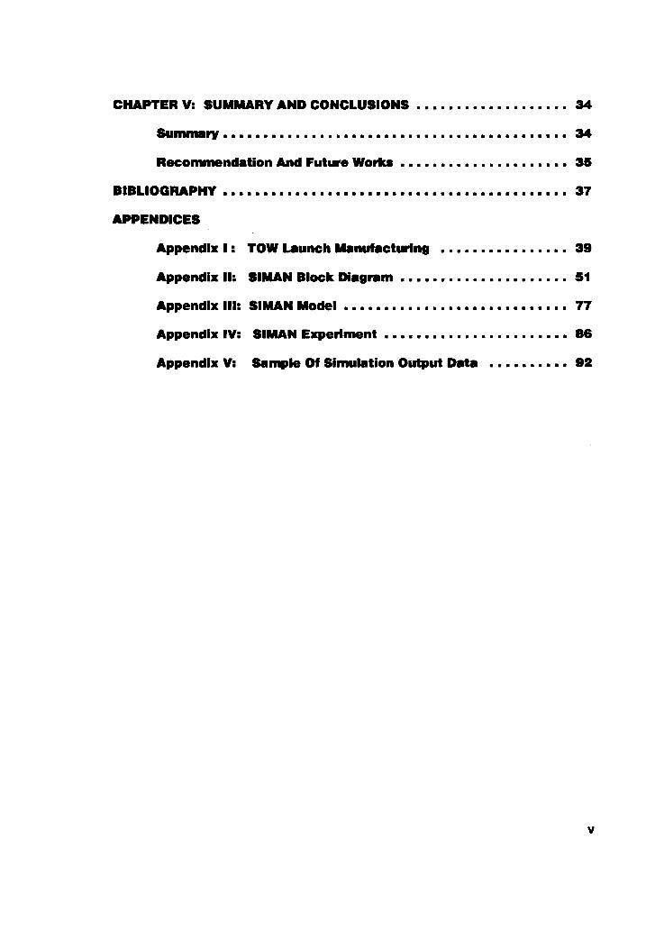
CHAPTER VI SUMMARY AND CONCLUSIONS ••••••••••••••••••• 34
SuIlMMI'Jf • • • • • • • • • • • • • • • • • • • • • • • • • • • • • • • • • • • • • • • • • •• 34
Recommendation And Future Works ..................... ••••••••••••••••••••••••••••••••••••••••••• BIBLIOGRAPHY
APPENDICES
Appendix I: TOW Launch Manufacturing ••••••••••••••••
35
37
39
Appendix II: SIMAN Block Dla.l1Im ••••••••••••••••••••• 51
Appendix III: SIMAN Model •••••••••••••••••••••••••••• 77
Appendix IV; SIMAN Experiment ••••••••••••••••••••••• 86
Appendix VI Sample Of Simulation Output Data .......... 82
v

Figure 1
Figure 2
Figure 3
Figure 4
Figure 5
Figure 8
Figure 7
Figure 8
Figure 9
Figure 10
List Of Figures
RAAP Process Flows • • • • • • • • • • • • • • • • • • • • • • •• 2
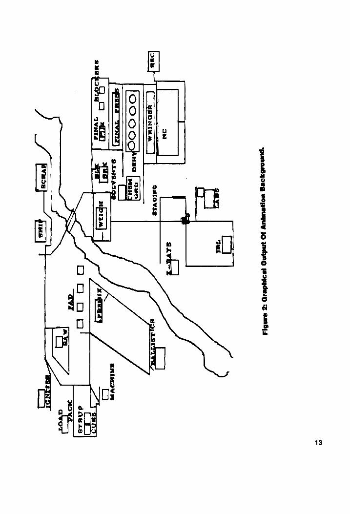
Graphical Output Of Animation BackgrolBld. • • •• 13
Green Lines Operations Combined For Simulation
Model. • • • • • • • • • • • • • • • • • • • • • • • • • • • • • • • • •• 18
Rocket Area Operations Combined For Simulation
Model. • • • • • • • • • • • • • • • • • • • • • • • • • • • • • • • • •• 19
Green Lines Manufacturing: Flow Chart For 117
Propellant For TOW Launch Motor • • • • • • • • • • •• 41
Rocket Area Manufacturing: Flow Chart For TOW
LaulICh Motor •••••••••••••••••••••••••••• 42
M71ITOW 1991·1992 Green Lines Area Rework • 45
TOW Scrap • Sawing Operation
Rocket Manufacturing Area 1991·1992 •••••••• 48
TOW Scrap • Machining Operation
Rocket Manufacturing Area 1991·1992 •••••••• 49
TOW Scrap • X·ray Operation
Rocket Manufacturing Area 1991·1992 •••••••• SO
vi

Table 1:
Table 2:
Table 3:
Table 4:
Table 5:
List Of Tabl.s
Existing And Reduced Resource capacities •••• 21
Summa" Of Slmu .. tion Output Data
Average Queues And Utilizations For Base
Model ••••••••••••••••••••••••••••• 28
Tabulated Results For Throughput After A 50%
Reduction ••••••••••••••••••••••••••••••• 28
Summa" Of Simulation Output Data
Average Queues And Utilizations For SOCM.
Reduction Before Adjustments Were Made To
AOV'. And Machining Stations ••••••••• 30
Tabulated Results For Throughput After A ~
Reduction Of Resources and Adjustments Are Made to
Bottlenecks • • • • • • • • • • • • • • • • • • • • • • • • • • • • •• 32
vII

CHAPTER I: INTRODUCTION
OVERVIEW
The Radford Army Ammunition Plant (RAAP) Is located next to Blacksburg In the state
of Virginia. This plam Is a "Govemmem Owned-Company Operated" or a GOCO plant.
Hercules Incorporated has been the contractor for this plam since It's origination on August
16, 1940. At that time, Hercules was the second largest manufacturer of smokeless powder.
The facility covers 2,400 acres of land, comalns more than 400 manufacturing buildings, 26
storage areas, and 156 other structures such as laboratOries, office buildings, bunkhouses,
firehouses, cafeterias, guard stations, and a hospital. There are forty-three miles of roads,
17 miles of fence, 12 miles of railroad track, and 800 miles of telephone wires on the plant.
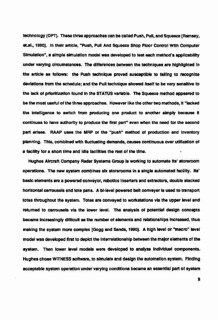
There are over one hundred different types of propellant and supponlng products
which It Is capable of manufacturing. Figure 1, RAAP Process Flows, depicts the main flows
of the basic products presently produced at the plant. All propellants produced are derived
from three basic types of smokeless propellant • Single base, Double base, and Triple base
propellant. The names come from the number of different constituents which make up the
energetic ponlon of the propellant. The energetic ponlon of the Single base propellants Is
Nitrocellulose. The energetiC ponlons of the double base propellant are Nitrocellulose and
Nitroglycerine. The energetic ponlons of the Triple base propellant Include NltroGuanadlne
as well as the constituents of the Double base propellant.
1
ACID AREA
AWWOHIA
• can. ... <1-___ -.. NoSTIC ram mp Figure 1: lIMP Proce .. Flows
It o LP LO a_ DD • a
2
Propellant can be manufactured by using the Solvent less. cast, and/or Solvent wet
processes. In the Solvent less process. the propellant Is blended while It Is In the fonn of
a water wet paste prior to funher processing. The cast process Is used to make large
propellant grains from smaller components In a mOld. The process of most Interest for this
paper Is the Solvent wet process. The M7 propellant used to make TOW Launch grains Is
made using the Solvent wet process. The process Involves mixing propellant Ingredients
with a solvent mixture containing combinations of Dlethyl-ether and acetone. A more
detailed description of the process can be found In Appendix I of this repone Other
propellants may also use alcohol In this solvent mixture as well. The solvent Is used to
enhance the mixing process and create a homogenous dough. The propellant Is extruded
Into Its' desired form and solvent Is almost completely driven out of the propellant.
The facility was built In the 1940's to suppon World War II eftons. It was designed fo ..
extremely high volume, batch manufaCturing. At full capacity, the facility employed as many
as 9,000 people late In 1941. Between 1941 and 1945, Hercules produced 1.2 billion pounds
of smokeless powder, 828.6 million pounds of TNT, 27.7 million pounds of Pentollte (a
special high explosive used with TNT), and 159.2 tons of anhydrous ammonia.
Presently due to the cut backs In defense spending, much smaller and more varied
orders are being procured with much less efficiency per pounds than seen In the past.
Presently, production orders require under one hundred thousand pounds of propellant per
month and all resources are vastly under-utlllzed. Therefore, production planning Is almost
non-exlatent. Due to this lack of planning, operators and resources are constantly being
utilized at high capacities and then closed down completely. This Is also due to the use of
the traditional "large batch" processing method of manufacturing which the plant Is
accustomed to using In the past. Most of the products being produced on plant today are
3

In their mature or declining IHe cycles. In the future, the plant will need to change to
accommodate new developing products and relatively small orders, or It will be forced to
close due to extreme Inefficiencies caused by Its' original design.
It would be beneficial to develop an animated simulation model of this process to help
management evaluate changes In future operating strategies. The model also provides a
training tool to Illustrate the processes Involved for producing propellant. The model
provides Information on work-In-process Inventories , utilization of resources, and the
output of materials. A simulation modelling approach should be used so that cycle times,
scrap rates, and rework rates can be Investigated using probabilistic values.
Problem and Objective
This project focused on the manufacturing processes required to produce the TOW
Launch propellant. There are 30 separate operations required to produce TOW Launch
propellant. A detailed description and a flow diagram of these operations can be found In
Appendix I, Figure 5 and 6 of this repone Presently, 72 mixes (one HPC lot of cotton) Is
releasect for production (approximately every four month period) to fulfill present
requirements. This project Investigated and defined the resources necessary to suppon a
50% reduction In demand. Alternative equipment configurations were Investigated using
the simulation model to detennlne the minimum resources needed to meet required
shipping schedules. The primary performance measure examined was the percentage of
shipping requirements attained by the total resources. Actual shipping requirements,
capacities, etc. are Information which should not be disclosed due to proprietary or security
reasons. Queues and resource utilization were examined to Identify opponunltles for
resource reduction.
4

Due to government regulations, each batch processed through the Forced Air Dry
operation Is considered an HPC lot. Each HPC lot Is subjected to a series of expensive
ballistic testing. If lot sizes are reduced, the cost per pound of propellant (for ballistic
testing) will be higher. However, this cost may be offset by the reduction In total system
CYCle time, or the decrease In fluctuation of utilization of manpower. Cost Is addressed only
Indirectly through minimization of resource requirements In this study_
5
Chapter. I.: Review of Applicable Uterature
U.Nlne_ of Simulation As An Analytlca' Tool
Simulation Is becoming Increasingly more Imponant as a tool for the manufacturing
environment. As hardware and sottware capabilities become more extensive and less
expensive, the cost of simulation become less significant compared to the returns which
simulation can offer. Simulation can be helpful to a business throughout Its' life cycle (Ie.
stan-up, growth, maturity, and decline). As a business progresses through each of the
phases of It's cycle, the material handling needs change 88 well as the resource
requirements. During the earty stages, the batch process Is preferred 80 that the business
Ia flexible to the customer's needs. But as production demands Increase, batch processing
may become less feasible. Simulation can be utilized during the Investigation of alternative
mode of operations. Black Diamond Corporation W88 observed to use simulation to
Investigate effects of making changes Involving layouts, batch sizes, purchase of new
equlpments, reduction of down time for equlpments. and elimination of rework operations
[J. lewis, 1991).
Foreign competitors have motivated U.S. companies to be more productive and quality
has become a more Important marketing strategy than price. The key to maximizing both
profits and productivity Is by control of Input costs and by using efficient processes. A
small business has a more difficult time doing these things while preparing for expansion
than a large government owned Installation like RAAP. At the stan, a small business
produces products In a batch process. However, It Is during the growth stage that Internal
6

efficiency and qualHy becomes vulnerable. Simulation combined with Industrial engineering
principles can boost productlYHy In such casas [J. lewis, 1991]. At RAAP, the reverse Is
taking place. In the past, the Internal Inefficiencies and the lack Of quality which were
nonnally absorbed by high volumes will no longer be tolerable In future smaller production
lots.
Detemdnlstlc Approach
At each operation, parameters such as batch sizes, cycle times, or available resources
can be altered to examine the system's performance. H each of these parameters are only
examined at two levels each, the number Of factors would be 90 (for 30 stations and three
parameters), at two levels each would make the number of combinations 2'" or 1.238x1cf1.
Even If a designed experiment such as the Taguchl method were to be Investigated, the
design which would be used would be an 1.,21 (onhoganal array consisting of 128 rows and
128 columns used to evaluate 128 factors with two levels each) and the minimum of 128
experiments would be required for each replication. However, through closer examination,
InteractiOns must be considered because changing one factor may affect the qualHy of the
next operation and thus affect the other factors. The 1.,21 design will only allow for 37
Interactions. H there are any more Interactions than 37, the next design matrix would be an
t... which would consist of 256 experiments for each iteration. The analysis Is funher
complicated because the system's perfonnance can be measured In tenns of costs, queue
sizes, utilizations, output, or quality. Therefore, a delemalnlstlc approach to this problem
would require many experiments and large amounts of data reduction.
R. J. Reynolds Tobacco Company, a subsidiary of RJR NabiSCO, used simulation
methodology to solve Similar material handling problems due to the complexity of a
7
deterministic mOdel. They conducted a study to determine the In-process storage
requirements for a proposed material separation process. nals process Involved ,the
separation of composite material from manufacturing Into Individual components. A
computer simulation was developed that followed the flow from the manufacturing floor, to
a composite material storage area, to a material separation line, to a component storage
area, and back to the manufacturing floor. Lotus Imponed the file of data from the
simulation and created an XV graph of time versus number of containers In storage. The
benefit of using simulation allowed the company to play 'what If' games with Input
parameters. As a result of the simulation, management discovered that they would need
more physical space to accommodate 995 containers If they adopted a newly proposed
material separation process. The separation process was previously done off plant which
required excessive material handling and quality controls [R.E. camp, 1993].
The previous example seems almost overly simplistic. However, It points out how
efficient simulation can be for determining the storage capacity requirements as opposed
to a deterministic approach. A warm up period of eighteen days was required to
accumulate a "normal" level of containers required because the simulation staned wHh an
empty queue. nae statistics used for the simulation was kept simple but effective. The
software package WITNESS was used to build the model. The results showed exactly how
many containers could be accommodated In each area and how many hours wonh of
composite material would be segregated In one shift.
Meterials Hanellina Cases
Factory production and Inventory control Is generally handled In three ways: material
requirements planning (MRP), Kanban or 'just In time' (JIT) , and optimized production
8
technology (OPT). These three approaches can be called Push, Pull, and Squeeze [Ramsay,
at.al., 1990]. In their article, "Push, Pull And Squeeze Shop Floor Control With Computer
Simulation", a simple simulation model was developed to test each method's applicability
under varying circumstances. The differences between the techniques are highlighted In
the article as follows: the Push technique proved susceptible to failing to recognize
deviations from the schedule; and the Pull technique showed Itself to be very sensitive to
the lack of prioritization found In the STATUS variable. The Squeeze method appeared to
be the most useful of the three approaches. However like the other two methods, It "lacked
the Intelligence to switch from producing one product to another simply because It
continues to have authority to produce the first pan" even when the need tor the second
pan arises. RAAP uses the MRP or the "push" method of production and Inventory
planning. This, combined with fluctuating demands, causes continuous over utilization Of
a facility for a shon time and Idle facilities the rest of the time.
Hughes Aircraft Company Radar Systems Group Is working to automate ItS' storeroom
operations. The new system combines six storerooms In a single automated faCility. ItS'
baSic elements are a powered conveyor, robotics Inserters and extractors, double stacked
horizontal carrousels and tote pans. A bl-level powered beH conveyer Is used to transpon
totes throughout the system. Totes are conveyed to workstations via the upper level and
retumed to carrousels via the lower level. The analysis of potential design concepts
became Increasingly difficult as the number of elements and relationships Increased, thus
making the system more complex [Gogg and Sands, 1990]. A high level or ''macro'' level
model was developed first to depict the Interrelationship between the major elements of the
system. Then lower level models were developed to analyze Individual components.
Hughes chose WITNESS software, to simulate and design the automation system. Finding
acceptable system operation under varying conditions became an essential pan of system
9
planning and this simulation helped speed the identification of possible flaws and defects.
System problems pointed out by this simulation could not be Intuitively IdentHled during
the planning stages. this anlcle was one of the most encompassing anlcles found on the
usefulness of simulation. It pointed out that tithe Investment of time. effon, and money In
this (simulation) planning process yielded a visibility of the future operating problems
without experiencing them In actual operation."
WITNESS, as described by these anlcles, resembles ProModel In that It Is a special
purpose simulator which concentrates on manufacturing and requires slgnHlcantly less time
to program than a general purpose simulator. These special purpose software systems
seem easy to use and yet they are not limited. Teledyne used PROMODEL Version 4.1 to
simulate the upgrade of a process of an entire facility to Include In-line computer
processing, prior to actual construction. The plant produced Nickel and TItanium
superalloys. A proposal was made to eliminate batch processing and assOCiated
Inefficiencies by linking each operation with a variety of conveyors. The whole simulation
was done on a CompuAdd 386 20 mHZ microcomputer with 2 megabytes of RAM, an 80
megabyte hard drive, and a VGA monitor [Marmon, 1991]. Questions to be answered by this
simulation were: how much faster Is In-line versus batch processing? How much more
capacity will be gained? And will reduced cycle times and Increased capacity Justify the
high cost of automated material handling? The objective was to provide results to aid In
the cleslg n and Justification of the In-line finishing cell.
Most anleles about computerized simulation focus on a panlcular case study or a single
manufacturing process. Simulation Is used In many manufacturing related activities at
Honeywell's Micro SWItch Division Simulation can be a flexible tool In diverse applications.
WITNESS, by AT&T .. ISTEL Corp, was chosen because of programming ease and adaptability.
Simulation at Micro Switch Is used In ways that Include Justifying new office equipment
10
(more CAD stations In this case), analyzing assembly processes for production or
productivity enhancements, analyzing fabrication equipment to reduce setup/changeover
time, assisting In production operation layout, and analyzing material handling systems In
multi-floor facilities. Situations reviewed here show how computerized simulation and
Industrial engineering skills can combine In beneficial ways [Dwyer and Korwln, 1990].
Simulation offered the solution to Hong Kong Air cargo Terminals Ltd (HKACT) as It
planned to acoommodate Terminal 1 overload and continue cargo growth. HKACT needed
to build the terminal vertically since land was scarce. In addition, HKACT needed to
evaluate system features quickly and carefully before the final design and construction,
since the Investment was enormous, the design was unique and other ~ons.
AutoSlmulatlon's Auto Mod II silicon graphics workstation was used and the accurate,
detailed mOdel was completed In just three months. Simulation made It possible to predict
potential problems with a degree of accuracy and solve them before the terminal was built
[Luk, 1990].
The two main systems that were examined at HKACT were the Bulk storage system
(BSS) and the Container storage system (CSS). The simulation mode' of the BSS
concentrated on the feasibility of the proposed control log Ie, queuing problems at the Input
and output (110) areas, management of empty box and bins, scheduling of stacker cranes,
and utilization of storage racks. Simulation mOdels of the CSS examlnecllnvestlgatlon of
the utilization and operation cycle time of high-speed elevators, empty container elevators,
and floor level shuttle cars. Examination of the storage capacity, detection of specific
bottlenecks, and what· If analysis evaluating control strategies for material flow were also
simulated.
11
The aeneflts of Anlmlltlon
Simulation modeUng Is growing In popularity, due In large pan to the easy-to-use
animation [Law, 1991]. Animation's chief appeal Is Its' ability to communicate the "crux"
of a simulation. Animation represents key elements of a system on a computer screen as
Icons. These Icons change color, shape or position with a change In the simulation.
Animation also allows for a way of debugging of a simulation program. It can show when
• simulation model Is Invalid and can encourage suggestions to Improve the system.
Animation makes It easier to understand the behavior of a system and makes It easier to
train operational workers. However, animation should not be used as a substitute for
careful analysis of data output by the simulation.
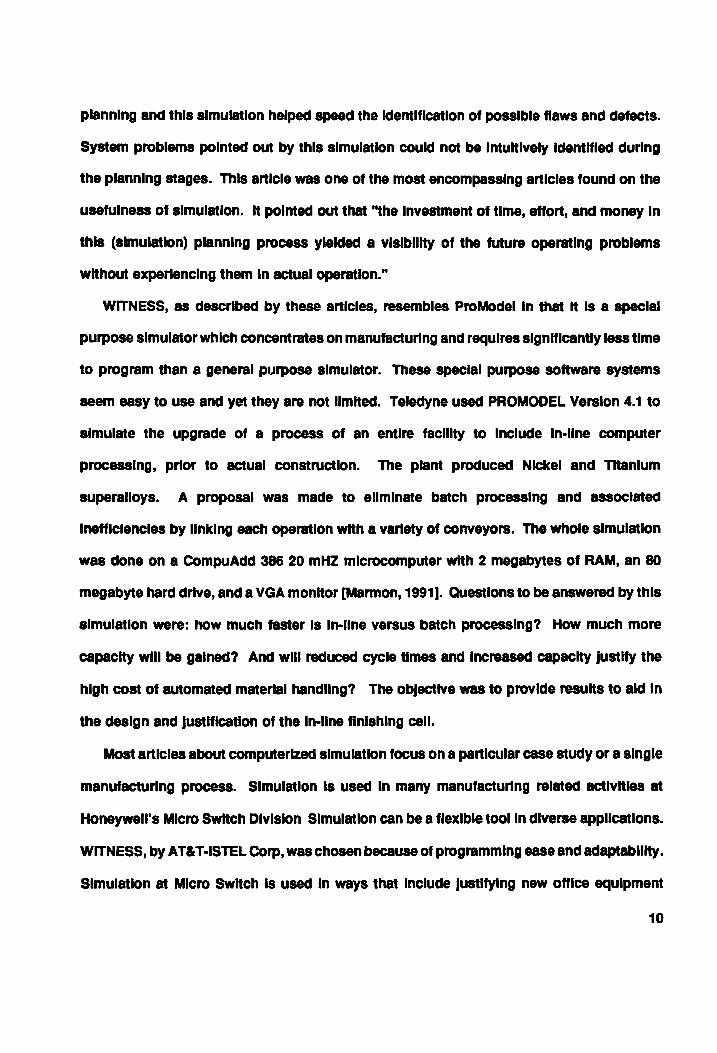
Animation fOr the model proved to be especially useful for this project. During the
development of the model, animation was not only useful In detecting the blocks where
problems with the code arose, but It also proved useful during model validation. Someone
who Is familiar with the process can, by examining the animation. verify the accuracy Of
how the model depicts material movement moves through the process at RMP. For
Instance, although the data output gathered were statistically correct In one model,
animation was used to detect an unlikely traffic problem while the AGVs were In route.
Animation also makes presenting this model to management a lot easier. A graphical
output of the project's animated background Is Illustrated In Figure 2: Graphical OUtput Of
Animation Background.
12
t J i
) o
i 1 i ! CJ Q
i
13
About •• MAN And Cinema
SIMAN IV Is a powerful. general-purpose simulation software package which Is equipped
with capabilities to expand through Its' link with FORTRAN. It Is capable of network
modeling, discrete event scheduling, continuous modeling or a combination of these for
combined dlscrete-contlnuous models.
The SIMAN software divides the model Into two pans - the "model" and the
"experiment". This allows the user to change parameters and variables using only the
experiment section of the mOdel. In the experiment section of the model, the user may
change parameters such as the batch sizes, the time between cotton batch releases, the
time between NG manufacture, the time between chemical preparation. the nurrlber of
resources for each station, the mix sizes, the cycle times at each station, the number of
vehicles to be used, the number of operatorsllnspectors available, and the speed limit of the
vehicles. "while changing the cycle time or mix sizes, the rework or scrap rates change
for the Final Mix or the Sawing Operation, the user may also make adjustments to these
variables accordingly.
This "model" component and "experiment" component framework Is based on the
theoretical concepts developed by zeigler (1976). The model describes the physical
elanents of the system (machines, workers, storage points, transponers, Information, pans
flow, etc.) and their loglcsllnterrelatlonshlps. The experiment specifies the experimental
conditions under which the model Is to run, Including elements such as Initial conditions,
resource availability, type of statistics gathered, and length of run. The experiment frame
also Includes the analyst's specifications for such things as the schedules for resource
availability, the routing of entities, etc. Experimental conditions are specified external to the
14
model description 10 that they can be changed without modifying the basic model
definition.
Once a model and experiment have been defined, they are linked and executed by
SrMAN to generate the simulated response of the system. As the simulation Is executed,
SIMAN automatically saves the responses specified In the experiment. The SIMAN Output
Processor can then be used to generate plots, tables, bar charts, histograms, correlograms,
and confidence Intervals from the saved data. The data can also be displayed by using
commercIally available mainframe, ml,lIcompute,. or microcomputer presentatlon-qualHy
graphics packages.
SIMAN Is supponect by Cinema for Its animation. The user builds the animation layout
by USing a bullt·ln drawing package In Cinema or layouts can be Imponed from AUTOCAD
DXF files. Entities, Queues. Resources, etc. must be defined the same as appears In the
SIMAN program. The user links the SIMAN program with the Cinema animation on the last
line of the experiment section of the program. CSIMAN pan of the software runs the
animation and allows the user to see a real time graphical animation of the SIMAN model
with Jobs or customers moving through the system.
The Advanced Manufacturing Systems Division (AMSD) at Cincinnati MllBcron Is taking
on an Increasing amount of engineering consulting work. Since 1966, the division has
designed numerous flexible manufacturing systems. At present, Cincinnati Mllacron Is
modernizing a facilHy for a European aerospace manufacturer. AMSD makes extensive use
of the SIMAN modeling language. In the late 19708, AMSD developed Its own Fonran-based
Simulation model and used It for nearly a decade. this program contained about 15,000
lines of code and was very difficult to use and maintain. Now with the help of SIMAN,
simulation can be used more readily and more frequently. The reasons for the growing
popularity of computer simulation Is that It Is not time consuming, It Is Inexpensive, and
15
there are an Increasing number of customers who will not buy a major manufacturing
system, let alone a facility, without having been shown some kind of simulated results.
Another heavy user of SIMAN Includes Westinghouse Electric Operations Systems (OS)
group. It uses simulation to decide whether an Improvement to the plant, or expansion, or
technology should be the course of change It wants to seek. A model was developed to
track truck movements at ground level and subterranean level In the Waste isolation Pilot
Project (WIPP) In carlSbad, New MexicO [Industrial Engineering, June 1990]. AUTOCAD and
other CAD schematiCS were typically Imponed Into the Cinema package for animation.
SIMAN was chosen as the simulation language and Cinema was used to animate the
simulation. Although the software chosen proved to be a powerful package, the ma.ln
reason for this choice was It's availability at Virginia Tech.
16
CHAPTER III: APPROACH TO THE PROBLEM
Modelling Methodoloav
The purpose of this project Is to Illustrate to the user a method of Investigation for
different alternatives for the material handling and the manufacture of TOW Launch
propellant. The 30 operations required to manufacture TOW Launch propellant are
performed In two different areas. Currently, one HPC lot of cotton (72 mixes) Is released
for production (approximately one every four months). The first 13 operations are
performed In an area of the plant referred to as the "Green Lines". Each mix Is transferred
to the "Rocket Area" where the remaining operations are performed. Each entity In the
model represents a mix In the Green Lines or a Sublot In the Rocket Area. Each operation
has been simplified to a basic cycle time which Includes pans handling, average setup, and
processing time so that the whole process can be examined at a macro level. Maintenance
Is perfonned during Idle periods. Each cycle time was examined and found to be
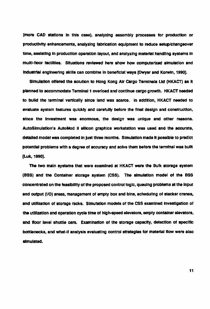
distributed Lognonnally with mean J.L and variance er. In order to simplify the model, some operations were combined, when poSSible, without
Invalidating the mOdel. The Pressing, CUtting and Boarding operations were combined
because they all take place at the same station, and one Is done Immediately after the other
to the same mix. Therefore, these operations can be viewed as one operation with one total
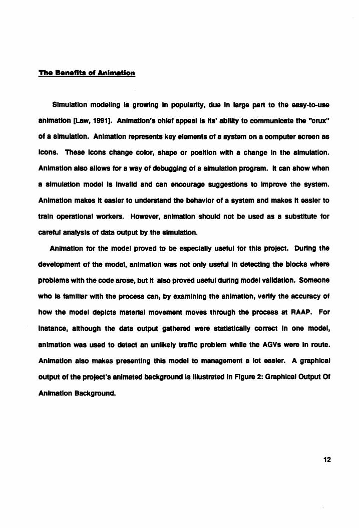
cycle time from a systems view point. Operations 16 through 21 and operations 25 and 26
were also combined for the same reasons. Therefore, 30 operations were reduced to 22
17
Conan Linten
Rocket Area
Fig .... 3: Green Lines Operations Combined For Simulation Model
18

From Green Unes
I~~~I fay
.... , Fig .... 4: Rocket Area O .... tlon. Combined For Simulation IIocIeI
19

Operations for the model and their cycle times adjusted accordingly. Figures 3 and 4
Illustrate the operations which were combined.
Table 1 Illustrates the resources and their capacHles for operations after they have been
combined for modeling. At each resource, the actual cycle time Is not published for
proprietary reasons. "a fifty percent rac:luctlon In demand was anticipated and the
resources were to be rac:luced accordingly to approximate proponlons. the resuHlng number
of resources and their capacity Is presented In the third column. At some operations. a
50% reduction does not affect the number of resources because only one Is presently being
used. Other resources will be reduced by more than SOO~ because an odd number Is being
used. The resulting scenario will be simulated to detennlne H the reduced shipping
schedule can be supponed by the reduced operating capability. Adjustments will then be
made as necessary to identity the minimum resources needed to suppon required shipping
schedules.
Some operations requlrac:l external production material as In the case of the Mixing
operation which required Nitroglycerin, and the Turkey Basting operation which required
syrup were assumed to have other production systems In place to handle the needed
material. This assumption can be made because there have always been plenty of these
auxiliary materials In stock and they have never been the bottleneck In the past. However,
In the future this model can be modified to predict how much of these materials are needed
and at what Interval so that a just-In-tlme type production plan can be Implemented.
AutomatiC Guided Vehicles are used to simulate trucks because the distance constraint
requirements between vehicles while In route could be handled more easily using zone
requirements already present In AGV movements built Into the software. Otherwise, the
movements of the AGV's on a two way track are identical to that of the ''truck like" vehicles
In actual use. At the beginning of the simulation, the AGV's all stan In the middle of the
20

Ope ... tlon
o AGV Trans.
1 Receiving 2 Ne MIg 3 Wring 4 Dehy 5 Block Brk 6 Cotton Wt. 7 Premix 8 Final Mix 9 Blocker 10 Press+Brd. 11 FAD 12 Sawing 13 Machine 14 Preparation 15 Pin 16 CUre2 17 X-ray 18 Turkey Bst 19 Bag 20 Weigh 21 Motor Ld 22 Ship
Table 1: Existing And Reduced Resource CIIpacltles
Number of Resources Presentl, Available and Their Capacltv
5 capacity = 1 Mix each or 4 sublots only after FAD 1 capacity = 1 Mix each 1 capacity = 1 Mix each 2 capacity = 1 Mix each 2 capacity = 1 Mix each 2 capacity = 1 Mix each 1 capacity = 1 Mix each 4 capacity = 1 Mix each 2 capacity = 1 Mix each 2 capacity = 1 Mix each 6 capacity = 1 Mix each 4 capacity = 72 Mix each . 1 capacity = 1 Mix each 2 capacity = 1 Mix each 3 capacity = 1 Mix each 3 capacity = 1 Mix each 3 capacity = 1 Mix each 1 capacity = 1 Mix each 3 capacity = 1 Mix each 3 capacity = 6 Mix each 2 capachy = 1 Mix each 1 capacity = 4 Mix each 1 capacity = 4 Mix each
~Reductlon
2 capacity = 1 Mix each or 4 sublots only after FAD 1 capacity = 1 Mix each 1 capacity = 1 Mix each 1 capacity = 1 Mix each 1 capacity = 1 Mix each 1 capacity = 1 Mix each 1 capacity = 1 Mix each 2 capacity = 1 Mix each 1 capacity = 1 Mix each 1 capacity = 1 Mix each 3 capacity = 1 Mix each 2 capacity = 72 Mixes 1 capacity = 1 Mix each 1 capacity = 1 Mix each 1 capacity = 1 Mix each 1 capacity = 1 Mix each 1 capacity = 1 Mix each 1 capacity = 1 Mix each 1 capacity = 1 Mix each 1 capacity = 6 Mix each 1 capacity = 1 Mix each 1 capacity = 4 Mix each 1 capacity = 4 Mix each
21

plant at a "staging" area. This Is a reasonable estimate of their average posnlon because
when the lot Is rel8888cl for production, the vehicle would enher be at the staging location
or scattered throughout the plant completing other tasks. All vehicles check to see H they
are needed at another station Immediately after every delivery. H so, they service the next
station without staging. If not, they return to the staging area. The number of stagings are
counted to detennlne If adequate staging Is being perfonned and H a reduction In the
number of AGVs are possible. OUtput for AGVs Include the percentage of "buSy" time as
well as the percentage of "active" but not delivering times. This simulation of staging Is
acceptable because operators telephone the central office prior to leaving a serviced
station. H there Is no station of the same product to Immediately service, the driver
prepares the truck to service another product or returns to the staging area.
The plant operates 24 hours per day, 7 days per week. Each simulation time unn In the
model represents one hour. The model was run for a simulated four months period or 2880
simulation hours. The data and some of the processes presented for the model has been
aHered to protect any proprietary Interest of Hercules Incorporated or RAAP.
During the actual operation, the mixes are blended to make the same number of sublots
at the FAD and Sawing operation. This Is simulated and described In the next section. This
blending affects the unHormlty of the reject rates throughout the lot and Is simulated In the
SaWing, Machlrllng and X-ray operations.
Model Description
The block diagram and the code for the model are found In the Appendices. The model
begins with the creation of batches of cotton, wnh time between arrivals exponentially
distributed, to be Inspected at the Receiving station. Throughout the code each Inspector
22
or each operator represents one resource (Ie. they operate one unit of resource). An AGV
Is then requested and the cotton Is transponed to the Nitrocellulose manufacturing station.
Here an operator and an Inspector are required to monitor the process until a batch Is
made. The operator and the Inspector Is released and the material Is sent to the wringer
queue. The wringer only processes one mix a time. The AGV picks up the processed mix
from the Wringing station and transports It to the Dehydration station where the animation
attribute Is changed.
The mix Is then sent through the Block Breaking, Cotton Weigh, Premix, Final Mix, and
Blocking operation using similar mechanisms. At the Final Press and Boarding operation,
the yield Is about 64 percent and the remaining 36 percent Is sent back to the Final mixing
operation to be reprocessed as simulated wtth a branching node.
The good materials are sent to the Forced Air Dry (FAD) operation where a whole HPC
lot Is accumulated prior to processing. The mixes walt In the FAD queue prior to being
combined and processed through temperature cycling. Once this Is completed, a sample
Is sent (via vehicle) for ballistics evaluation. this IS a destructive test so the sample Is
"dispOsed" at the Ballistics lab. The remaining materials are divided Into sets of four
"sublots" and walts In an "FADdone" queue for a signal to be given from the Ballistics lab
(via telephone). After the signal Is received, one set Of four sublote are sent to the Sawing
operation. After the Initial Signal, the remaining release signals for the lot are given by the
Sawing operation.
At the Sawing operation each set Is divided Into four Sub lots. The SawIng operation
processes one Sub lot at a time until all tour have been processed at which time It sends a
algnal to the FADdOne queue to send another set of four SUblats. At this operation the
material Is Inspected and the rejected material Is sent to the Burning Grounds for disposal.
23

The good material Is sent to the Machining operation. At the Machining operation, the
rejected grains are also sent to the Bumlng Grounds for disposal. The remaining materials
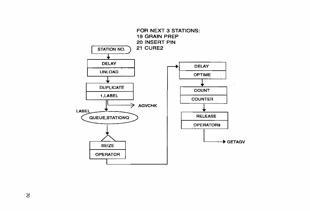
are then routed to the Grain Preparation, Insen Pin and the CUring operations.
During the cure time the operator Is Idle. After curing, the materials are transferred to
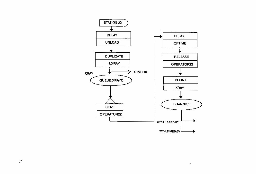
the X-ray operation. Here the grains are Inspected Intemally and the reject grains are
disposed of at the Burning GroundS. The good grains are transferred to the Turkey Baste
where Basting and CUring of the grains are both done In this operation. After this Is done
the materials are transferred to the Bagging, Weighing, Motor loading, and Shipping
operations. These operations are simply a series of standard "Queue, Seize, Delay, and
Release" blocks. At the Shipping operation, a measure of ''tIme In system" Is taken (Tally)
and the entity Is disposed.
Performance CrIteria
The purpose of this Investigation Is to determine the minimum system resource
configuration necessary to suppon reduced production requirements without delinquent
shipment. Since this repon will not disclose the shipping requirements due to proprietary
Infringement, performance will be measured In terms of percentage of shipping
requirements fulfilled. The 'first model will be validated by Its' capability to produce 100
percent of the shipping requlrements,wlthln the 2880 time units allotted with 10 percent
variance on the surplus side and no variance on the delinquent side as this Is consistent
with the present production and shipping policies. Successive modHled models will be
measured by their ability to produce 100 percent of the reduced requirements with the same
variances. This policy of producing surplus Is In place because delinquent orders of
propellant may mean bottlenecks to more critical systems off plant, while surplus
24
production Is stored without cost In government owned magazines on plant awaiting the
next order. Queues and utilization resources (Including AGV's) at each operation will be
examined to Identify opponunltles for resource adjustment (decreases or Increases, 88
necessary).
25

CHAPTER IV: CASE STUDY RESULTS
Model V.lldatlon
A model of the system was developed and executed 80 that a standard batch of cotton
which contained 72 mixes of propellant was released at the beginning of a four month cycle.
The model was adjusted, by using better estimates of the distances between stations, 80
that at least 105 percent of the production requirements were met with a variance of 5
percent. Actual scrap and rework data for a one year period were averaged for use In the
model. Average queues and utilization of each operation for the model were compared to
estimated actual queues and utilizations. For operations which were combined, the average
of the total queues were estimated based upon historical experience. Once the model was
adjusted, the number of replications was determined by estimating, with 95% confidence.
that the average percentage Of required shipment Is only off by 1888 than 4.0 percent to
ensure variance requirement specKled Is met. The following equation was used:
n= (Zonale)2
Where Zon = 1.96 for the estimate of IJ. < 0.05
and e = 4.0
a = 4..5 for the ten Initial data points generated
Therefore n = 4.8 or at least 5 replications.
A typICal printout of the data for the model Is In the Appendix V. The average queues
and utilization for all resources was very low over the simulation time as expected. These
26
are summarized In Table 2. This number was calculated by taking the weighted time for
which the value persists during the simulation. Most of the time the resources sat Idle
because only one lot at a time Is released over a four month period. However, during the
time the material Is being processed through any panlcular pan of the system, that pan may
experience very high utilization and maybe even some queue build up. This Is recorded In
the "maximum" queue column. It Is observed that the highest maximum queue values
occur at the FAD and the Machining operations. Thl., again, Is very consistent with actual
practice. The high queue build up at the FAD occurs by design. The material Is purposely
accumulated there before the FAD bay Is turned on for efficiency reasons. The large queue
build up at the machining operation Is not significant because the average utilization for the
station Is less than 200" and, therefore, the queue may be eliminated through better material
handling or by better production control methods In the future. The AGV's (trucks In actual
practice) have the highest utilization of approximately 80%, which Is again eXPfCled and
consistent with actual practice because of the vast distance requirements between stations
due to explosion propagation safety practices.
Anal,sls Of Svstem and Doc ..... ntlation 01 Results
The resources for the model and the lot size were reduced by 500.4. The amount
produced at the end of 2880 hours of production was compared to the required demands
and the results of each of the replications are listed In Table 3. Since the standard deviation
27

Average Queu •• And UtiliZllllon For •••• Model
MAX AVERAGE IN AVERAGE
OPERATIONS QUEUE QUEUE OPERATIONS UTILIZATION
AGVQUEUE 0.00943 4.0 AGV 1 Time Active 0.87727 NC QUEUE 0.03642 6.0 AGV 2 Time Active 0.88215 NQ(NCPROCQ) 0.163 6.0 AGV 3 Time Active 0.87877 WRINGER QUEUE 0.000081 0.0 AGV 4 Time Active 0.87673 DEHYQUEUE 0.000073 1.0 AGV 5 Time Active 0.49915 BLOCK BREAK QUEUE 0.000052 1.0 AGV Actual Busy 0.80007 WEIGH QUEUE 0.00121 1.0 PREMIX QUEUE 0 0.0 RECEIVING STATION 0.100000 FINAL MIX QUEUE 0 0.0 NITROCOTTON STATION 0.249970 BLOCKER QUEUE 0.00375 1.0 WRINGER STATION 0.100600 FINAL PRESS QUEUE 0.00172 1.0 DEHYS 0.100260 REMIX QUEUE 0.000086 1.0 BLOCKBREAKS 0.099230 FAD QUEUE 14.51 36.0 WEIGHS 0.125490 FAD DONE QUEUE 1.009 9.0 PREMIX STATION 0.099910 NQ(SAWQ) 0.14776 3.0 FINAL MIX STATION 0.154170 NQ(MACHINEO) 2.3453 14.0 BLOCKERS 0.154170 MACHINE INSP.O 0 0.0 PRESS AND BOARD 0.153190 GRAIN PREP QUEUE 0.01229 1.0 FAD BAY 0.003570 NC(PINNINGC) 0 0.0 SAW STATION 0.098510 NC(CURE2C) 0 0.0 SAW INSPECTION 0.000000 NC(CURE2DONE) a 0.0 MACHINING STATION 0.185640 NQ(XRAYC) 0 0.0 MACHINING 0.023260 NQ(BASTEC) 0.02305 1.0 GRAIN PREP 0.176370 NC(BAGC) 0 0.0 PINNING STATION 0.044280 NC(CHARGEWEIGHC) 0 0.0 CURING BAY 0.044440 NC(MOTORLOADC) 0 0.0 XRAY STATION 0.044460 NC(SHIPC) 0 0.0 TURKEYBASTING 0.152040
BAGGING STATION 0.057340 CHRG WEIGHING 0.038030 MOTOR LOADING 0.037910 SHIPPING 0.038230 BURNING GROUNDS 0.011810
28

Table 3: Tabulated Results For Throughput After A ~ Reduction
Repllcatlon(n) Percent of Required
1. 100
2. 96
3. 100
4. 96
5. 96
6. 96
7. 96
8. 96
9. 100
10. 96
11. 96
12 96
13. 96
29
T8b1e 41 Avenage Queues And Utlliations For ~ Reduction Before Adjustments
Were M8de To AGV's And M8chinlng Sutions
AVERAGE AVERAGE MAXIN AVERAGE
OPERATIONS QUEUE QUEUE OPERATIONS UTILIZATION
AGVQUEUE 0.670490 12.5 AGV 1 Time Active 0.618285 NC QUEUE 0.111275 4.5 AGV 2 Time Active 0.568770 NQ(NCPROCQ) 0.164630 4.5 AGV Actual Busy 0.237100 WRINGER QUEUE 0.000000 0.0 DEHYQUEUE 0.000083 1.0 RECEIVING STATION 0.175075 BLOCK BREAK QUEUE 0.000304 1.0 NITROCOTION STATION 0.125075 WEIGH QUEUE 0.001237 1.0 WRINGER STATION 0.049155 PREMIX QUEUE 0.000000 0.0 DEHYS 0.049600 FINAL MIX QUEUE 0.000000 0.0 BLOCKBREAKS 0.050200 BLOCKER QUEUE 0.000087 1.0 WEIGHS 0.062330 FINAL PRESS QUEUE 0.000307 1.0 PREMIX STATION 0.049705 REMIX QUEUE 0.000000 0.0 FINAL MIX STATION 0.066665 FAD QUEUE 3.618550 36.0 BLOCKERS 0.066665 FAD DONE QUEUE 0.274475 9.0 PRESS AND BOARD 0.066910 NQ{SAWQ) 0.074585 3.0 FAD BAY 0.003470 NQ(MACHINEQ) 0.439230 8.5 SAW STATION 0.049725 MACHINE INSP.Q 0.000000 0.0 SAW INSPECTION 0.000000 GRAIN PREP QUEUE 0.023115 1.5 MACHINING STATION 0.094345 NQ(PINNINGQ) 0.000000 0.0 MACHINING 0.011810 NQ(CURE2Q) 0.000000 0.0 GRAIN PREP 0.091645 NQ(CURE2DONE) 0.000000 0.0 PINNING STATION 0.022775 NO(XRAYO) 0.000000 0.0 CURING BAY 0.022915 NQ{BASTEO) 0.010205 1.0 XRAY STATION 0.022965 NO(BAGO) 0.000000 0.0 TURKEYBASTING 0.070760 NQ(CHARGEWEIGHQ) 0.000000 0.0 BAGGING STATION 0.026640 NQ(MOTORLOADQ} 0.000000 0.0 CHRG WEIGHING 0.017725 NO(SHIPQ) 0.000000 0.0 MOTOR LOADING 0.017670
SHIPPING 0.017785 BURNING GROUNDS 0.007290
30

Is less than 2, the number of replications required was much less than 13 (per the above
method of calculation) to ensure the true average. The data Illustrates that the process Is
not capable of meeting the expected output of 100 percent with a ten percent variance on
the positive side. Therefore, the utilization and queue data for the process was examined
to identify necessary resource adjustments.
The average queues and utilization for each of these replications are summarized In
Table 4. These averages were obtained by Imponlng each replication Into a Lotus file and
averaging 13 replications (thlneen was arbltrarlly used because It Is larger than 5 which was
the minimum required). It was noted that the resources that had the largest maximum
queues were the FAD, AGV's, and Machining operations. Again. the FAD queue can be
discarded. One more AGV was added and one more machining station was added to this
model making a total of three AGV's and two Machining stations. The model was run again
for 2880 hours per replications and the amount produced was compared to the shipping
requirements. The results are tabulated In Table 5: Tabulated Results For Throughput After
A 5()Ok Reduction Of Resources and Adjustments Are Made to Bottlenecks. The results of
this model were compared to the results of the orlglnal model to see H a difference could
be detected between the two using a confidence Interval-t-test.
To determine If there Is any statistically slgnHlcant difference between one system or
the other, performance measures was evaluated using the palred-' confidence Intervs/test.
Althoug h other methods can be uaed to compare the two systems, this technique Is utilized
for two reasons. First, the varlance between the two systems for each iteration does not
have to be assumed as equal. They would have to be assumed equal for methods like a
two-sample-t method. Secondly, the data between one system and the other do not have
to be Independent. Only the data within one system need to be Independent.12
31
Tabulated Results For Throughput After A 509b Reduction Of
Resources and Adjustments Are Made to Bottlenecks
Repllcatlon(n) % of Required For % of Required For Difference (d,)
Adlusted Model Original Model
1 108 108 0
2 104 106 ·2
3 104 108 -4
4 104 106 ·2
5 108 104 4
6 108 104 4
7 104 104 0
8 104 104 0
9 104 104 0
10 104 104 0
11 108 106 2
12 108 104 4
13 108 106 2
calculations to detennlne If the difference (d) was slgnHlcant between the two system
were made using the following methods:
d.r SUM{ct.)/n
s(d)= SQRT«SUM(drd..J,)/n-1)
a(d..J= 8(d)ISQRT(n)
h= t.,,1-a12 s(d">
32

The results were as follows for a 0.95 confidence Interval on S:
d.vv=.462
8(d)= 2.73
n= 13
8(ct...>= 0.76
t...1....,.= 2.18
h= 1.65
C.I.=[-1.19,2.11]
Since the confidence Interval of the ''throughput performance measure" for the two
systems Is between -1.19 and 2.11,11 can be concluded with 95 percent confidence that this
Interval contains the difference of the average throughput for the two systems. However.
since the Interval contains a 0, It can be assened that there Is no difference between the
two systems.
33
CHAPTER VI SUMMARY AND CONCLUSION
.u ....... rr
The Radford Army Ammunition Plant was designed for extremely high volumes of
propellant manufacturing. Due to the recem cut backs In defense spending, the demands
for such high volumes no longer exists. However, the plant continues to operate In a high
volume mode. A method to determine the resources which can be eliminated as production
Is scaled down, and stili not be delinquent on any orders, Is required. This method would
help define the resource capacRIes under the present mode of operation.
A Simulation model was built to reflect the present modes of operation for a typical time
period. Animation of the model was used In conjunction wHh data analysis to help validate
the model. The demands and resources for the model was then reduced and the model was
run for the same time period. The output was measured In terms of percentage of demand
met. Adjustments were made so that the model would produce the required percentage of
demands which would be equivalent to the original system. This defined the new resource
capacity for the new demand under existing mode of operation.
It was found that the overall utilization of all stations are InslgnHlcant over the four
month production period simulated. However, during the time when the material Is actually
being passed through the stations, some stations experience queue build up. Due to the
present mode of operation at RAAP, facllRIes are continually being used at full capacity and
then shut down completely for extended periods of time. ntis Inefficiency has been
accepted In the past, but as the plant prepares to compete wHh other propellam
manufacturing plants, for a smaller propellant market, It will be forced to plan for more
eftlclem use of the faCilities. This could be accomplished through the use of a more
34
continuous production planning techniques. Simulation modelling principles could help In
this task.
Even though the utilization of the AGV's (trucks) were high, a large pan of the "active"
time on the trucks were due to staging. This could be prevented by planning operations so
that one station could be serviced right after another. There were 72 mixes and 22 different
stations In each simulation, which makes approximately 1584 separate moves the trucks
would have to make (not Including rework or scrap) to complete the lot. During this time,
there were an average of 1400 staging operations due to lack of demand while the truck was
already out. Eliminating some of this staging may reduce the demands for vehicles.
In the future, RAAP may look Into a more continuous mode of operation utilizing smaller
batches and better planning. Due to the lack of experience In this mode of operation,
simulation would be an Ideal tool for RAAP's future planning. Animation of the model will
also help In the presentation of the model to management and key production personnel.'
Recommendation And Future Work
Other parameters may be Investigated using this model. The success of a simulation
project Is dependent on the simulation knowledge which the participants share and by those
who will be Impacted by the results of the project. It Is usually the simulation user's
responsibility to show management the basic methodologies and principles, and the
benefits which can be expected through simulation. Although only one parameter was
Investigated for this project, this model could be used to explore the consequences Of
changing other parameters for each operation In the process. By varying parameters and
variables In the experiment section of the software, the user can Illustrate unlimited
numbers of possibilities for future Improvements. However, care must be taken to examine
35

all effects of changing each factor when Investigating other modes of operation. Changing
one known factor may have large effects on unknown parameters which may make the
model Invalid. For example, If the Mixing operation were to be examined closely, the cycle
time could be reduced by changing the mix size. Besides having effects on the arrival times
at the next operation, this would also change the quality of the material so that the rework
rates for the process would also have to be adjusted.
Another example Is If the Receiving operation was to be examined. If a controlled
change was made to the batch sizes, the cycle time would be affected. The quality clown
stream of the process may also be affected due to different batch sizes and, therefore, other
yields would be affected. Here, making a known change to one factor could Influence other
factors In ways which are unknown and are slgnHlcant to the model's validity. Therefore,
It Is recommended that parameters and variables In the model should only be determined
by someone who has sufficient experience with the process to detect other possible
process Impacts which may not be accounted for by the mOdel.
36
Bibliography
1. Banks Jerry, carson John S. II, and Ngo Sy John. Getting Staned With GPSSIH.
Annadale, Virginia: Wolverine Software Corporation, 1989.
2. camp, R.E., "Storage requirements are detennlned through the use of simulation
(case study at R.J. Reynolds Tobacco Co.}", Industrial Engineering. II v22 March'90
p44(3)
3. camp, Roben E., "Simulation determines storage requirements at Reynolds Tobacco
Company", Industrial Engineering. II v22 Jan '90 p28(4)
4. Dwyer, John and Korwln, Steve, "Honeywell puts simulation to work In multiple
arenas (Simulation In Manufacturing)", Industrial Engineering II v22 Oct'90 p33(4)
5. Gogg, Thomas and Sands, Charles D., "Hughes Aircraft designs automated
storeroom system through simulation application (Hughes Aircraft Company Radar
Systems Group)". Industrial Engineering. II v22 August '90 p49(7)
6. Law, Averill, M., ''The many uses of animation and graphics In simulation". Industrial
Engineering II v23 Jan '91 p20(2)
7. Lewis, Joseph F., "Simulation combined with IE principles can boost productivity
In small business", Industrial Engineering, II v23 July '91 p46(5)
8. Luk, Marla, "Hong Kong Air cargo Terminals to work In synch because of simulation
applications", Industrial Engineering, II v22 Nov'90 p42(4)
8. Marmon, Craig, "Teledyne Applies Simulation To The Deslg n And Justification Of A
New Facility", Industrial Engineering, II v22 March '91 p29(3)
37

10. Pagden Dennis C., Shannon Roben E., and Sadowski Randall P. Introduction To
Simulation Using SIMAN. Hightstown, New Jersey: McGraw-Hili, Inc. 1990.
11. Prltsker, A. Alan B. Introduction To Simulation Using SLAM II. West Lafayette,
Indiana: Systems Publishing Corporation, 1986.
12. Ramsay, Manln L., Brown, Steve, and Tablbzadeh, Kamblz, "Push, pull and squeeze
shop floor control with computer Simulation", Industrial Engineering. II v22 Feb '90
p39(5)
13. Walpole Ronald E. and Myers Raymond H. Probability and Statistics tor Engineers
and SCientists. New York, New York: Macmillan Publishing Company, 1989.
38

Appendix I
39
TOW Launch ... nut.eturina
The flow diagrams for the M7 for TOW Launch and the TOW Launch processes are
Illustrated In Figures 5 and 6. The main areas Involved for the production of TOW Launch
are the Green Unas, the Finishing Area and the Rocket Area. However, the process actually
starts out In the Nttrocellulose Area where approximately 12,000 pound batches of cotton
linters are nitrated at one time to make Nltrocotton (NC). After the nitration process,
samples are taken to the laboratory to analyze for the extent of nitration. Adjustments are
made to the batch and the material Is then transferred to the wringer In the fonn of a water
wet slurry. The wringer wrings out the water from the NC to approximately 14% moisture.
At this point the NC appears In as 8 white powder.
The NC Is then transferred to the Green Lines where further reduction In moisture Is
done at the dehydration presses. Here the NC Is loaded Into the presses In approximately
100 pound Increments. After the water has sufficiently been re'!'oved from the NC. the NC
become cylindrical blocks as a result of high pressures from the presses. A sample Is
taken to the chemical laboratory during this time to ensure proper dehydration of the NC.
The Ne Is then transferred to the block breaking station where It Is broken back up Into
a white powder for funher processing. The NC Is then taken to the Cotton weigh station to
be weighed to determine NG and chemical additions. A Total Volatiles test Is done during
Cotton Weigh to detennlne the amount of NC required to form a mix.
40
Colton L.inten
SOLVENTS
CHEML..AB
REMIX
LEOBND'
Conaol Sample
A.cc:eptance Sample
Quality Control Check: Point
Production Clec::i: Point
Fig .... 5: Green U_s ... nulactwtna Flow eMrI For 117 Propellent For
TOW uunch lIotor
41

M7 (StAoderdl
S)'nIp
LEGEND CaIIroI Sample
QC Caect PoiDI
Fllure 6: Rocket Are. M.nuf.cturlna Flow CIuIrt For TOW LIIunch Motor
42
The NC Is then transferred to the Premix Area where Nitroglycerine (NG) 18 added and
stirred In plastic tubs. Mix numbers are assigned to each mix and the contents are referred
to as "Premixes". The Premixes are transferred to the Green Lines where alcohol and
acetone (or solvents), and trace amoLints of other chemicals are combined and mixed In a
800 pound capacity mixer to make a homogeneous ITlixture. Each of these Ingredients are
purchased and are Independently Inspected. At this point, the material appears as a black
dough. The color comes from the carbon Black added at the beginning of the mix cycle.
The maximum amount of material which can be processed through the mixers are
dependent on the rate at which NC can be made and mixed Independently WIth NG and
carbon black. The rest of the chemicals and solvents do not limit the maximum production
rate or these have not been the limiting factors In the past. The Green Lines presently
produces approximately 500 to 600 pound mixes and releases In batch quantities of
approximately 72 mixes for each lot. For the purpose of this study. a lot can also be
released as approximately 36 mixes.
After the material Is processed through the mixing operation, It Is transferred to the
blocking operation where the mix Is pressed In a low pressure press and made Into
cylindrical "billets" approximately 4 Inches In diameter. These billets are then transferred
to the pressing operation where another venlcal press pushes the billets through a die to
make approximately 0.75 Inch strands WIth a single perforation through the center. During
this process, the operators Inspect the strands for surface Imperfections and/or blisters
caused by the die or air pockets In the propellant. The rejected ponlons of the strands are
cut off and sent back to the Mixing operation as "remix". The process nonnally produces
an average Of 36 percent remix. Figure 7 depicts the percemage of remix over a thlneen
month period. Although Figure 7 shows that the variance from month to month Is extremely
high, the actual amounts per production unit are very uniform. Due to accounting problems,
43
the remixes are not calculated accurately on a per month basis but Is accurate on a yearly
basis. The remix Is then mixed with the ''vlrgln'' mixes and are processed as a nonnal mix.
There are two mixers, two low pressure blockers, six four Inch presses, and one boarding
station. There are 5 +/- 3 boards per mix and 17 +/- 1 strands on each board. These strands
are placed on eight teet boards and sem to the Forcecl Air Dry (FAD) area to be dried In
heated bays.
One mix at a time Is carried to the FAD Bays and the lot Is released from the Green
Lines for FAD cycling In Increments of approximately 72 mixes, and It Is dried In the FAD
bays on the boards In which It was transported. Although this Is not labor Intensive, It Is
very time consuming. The process time through the FAD accounts for over eighty hours
of the entire total procesSing time. However there are 21 bays, each of which can hold
approximately three lots of propellant If needed. This operation Involves a series of
temperature CYCling until the proper total volatile (TV) level Is reaChed. This Is detennlned
by the laboratory which takes one day to obtain test results. Most of the volatiles are driven
from the propellant during this operation 80 the strands become hard and plastic textures
ready to be sawed.
Before the SawIng Operation can begin, the lot must first be evaluated using an
"evaluation" sublot. A sublot consists of randomly mIxed propellant grains from mixes.
There are approximately 280 grains In each sublot (accounted for In pounds). This sample
evaluation sublot Is ballistically tested prior to processing the rest of the lot.
Tha strands In the rest of the lot are then transponed to the sawing Operation where
they are sawed Into 14 Inch grains .. From this operation until the end, the grains are being
processed In what Is considered the "Rocket Area'l. During this operation the reject rate
Is approximately five percent as depicted from historical data on Figure 8. Most of the
rejections are caused by unacceptably crooked grains or grains with defective surfaces due
44

f1. CD 0 ...
ff. eI) ... ::s --ca
LL
>-.., --ca ::s 0
E;1
fI. e o ,..
'if (\I. ,..
,.. r--
1 I
I I .. I I .. • .. I .. f • -... ; • It
45

to pinholes ancllor other deformities. These scrapped grains are transported to the
Incinerator where they are disposed.
The good grains are then transported to the Machining Operation where three radial
holes are drilled Into the sides of each grain and the grains are reamed and face on one end
to accommodate an Insert called a "pin" In later operations. During this operation, the
reject rates are approximately five percent as depicted on Figure 9. Rejects at this
operation are mainly caused by machining difficulties encountered.
The grains are then transported to the Grain Preparation station where the grains are
cleaned and cured to prepare for the Pinning Operation. At the Pinning Operation, a plastiC
Jacketed pin Is dipped Into a syrup-solvent and Inserted Into the machined end of each
grain. The purpose of this pin Is to hold the grains In place during propellant burning In the
launch motor. The pinned grains are loaded Into cabinets containing trays and are
transported to curing bays In the Rocket Area to be cured.
Once curing has taken place, they are transported to the X-ray Operation to be Inspected
for Internal voids or defects. Voids or Internal defects may cause unsymmetrical burning
of the grains In the motor. At this operation, approximately twenty percent of the grains get
scrapped for this reason. Figure 10 depicts the historical data to be used.
After X-ray, the grains are transported to the '7urkey Baste" Operation. At this
operation the grains are placed Into a fixture with the unpinned end up. The same syrup
solvent used at the pinning operation Is Injected Into the perforation of the grains using a
basting syringe. The purpose of this Is to ensure that all areas between the plastic jacketed
pins and the grains are covered with syrup. The grains are cured at this station.
After Turkey Basting and cure, the grains are transported to the bagging operation. Here
the grains are placed In plastic bags to control moisture absorption during further
processing. The grains are then transported to the Charge Weighing station where four
46

grains at a time are weighed on a "Shadow Graph" scale to ensure that they meet
specification charge weight requirements.
The grains are finally transferred to the Motor loading station where they are loaded Into
launch tubes. These launch tubes are then sant to shipping.
There Is one 88W, two machining stations available (only one Is usually used), two
pinning statiOns. one curing bay. one X-ray machine, one Turkey Basting station, one
bagging station, one Charge Weighing station and one Motor loading station. Some
restrictions to material handling abliRles are that the trucks cannot carry more than 500
pounds of propellant at once, and that the trucks cannot be less than 30 feet span while In
route.
47

12% I :;> < i
10% [ZJ QUALITY FAILURE % 10% I .....
8%
6% 6% 6%
5% ·5%
4%
2%
0% I I « I. I , « I I , « , I I I I I I I I I I I I
o N D J F M A M J J A s o
Fig ... III TOW acnlP • .. wi .... Openltlon
Rock ........ IIC ............ 1991 • 1982
~

FI ...... TOW SC .... • MIle ........ Openatlon
Rocket Menufeclurlng are- ...... · .. 992
~

~
20%
15%
10%
5%
- ,"--.--~- - /' <
14% ~
12% 12%
~ QUALITY FAILURE %
14% 13%
12% fTTT7I rlllJ 12%
0% I I I I , I I I I J I I I " I I I " I I I I I I « I I ( , I
o N 0 J F M A oM J
,. .... to. TOW Sc,.. • X..., ....... tIon
Rock.t ....... cturlnl Area 1 .. 1 • 1 .. 1
J A S 0
Appendix II
SIMAN Block Diagram For The Code
51
01 t-.,)
CREATE
ASSIGN
NS=1: ANIM_ATT =1: M=4
I STAn! 4) ~
SEIZE
INSPECTOR4
DELAY
RECTIME
1 r"'1 RELEASE
INSPECTOR4
QUEUE ,14 )1
REQUEST
AGV(SDS)
TRANSPORT
AGV, SEQ
DELAY
UNLOAD
1, NC
II
SEIZE
OPERATOR4: INSPECTOR4;
DELAY
OPTIME
~ AGVCHK
NEXT PAGE

U1 (,.,i)
RELEASE
OPERATOR5: INSPECTOR4;
1
SEIZE
OPERATOR5: INSPECTOR4
i
WRINGTIME
ASSIGN
AN I M_ATT=2
RELEASE
OPERATOR5: INSPECTOR4
~-..... GETAGV
REQUEST
AGV(SDS)"M
TRANSPORT
AGV,SEQ
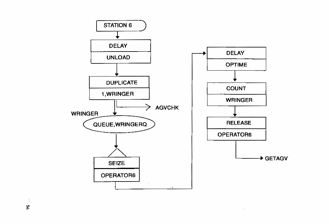
STATION 6 )
~ DELAY
DELAY UNLOAD
OPTIME
DUPLICATE ~
COUNT 1,WRINGER
I WRINGER'" ) AGVCHK
WRINGER
~EUE.WRING~ RELEASE
1 OPERATORS
LGETAGV SEIZE
OPERATOR6
~

01 01
STATION 7 )
+ DELAY
UNLOAD
DUPLICATE
1,DEHY
DEHY ~ ') AGVCHK
~EUE'DEHY0
1 SEIZE
OPERATOR?
DELAY
OPTIME
T RELEASE
OPERATOR7
~ COUNT
DEHY
~ ASSIGN
M=?
... GETAGV
(J1 0'1
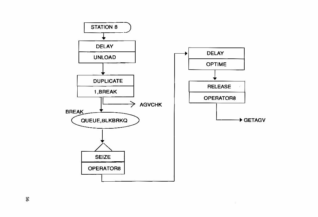
STATION 8 )
l DELAY
UNLOAD
DUPLICATE
1 ,BREAK r ') AGVCHK BREAK - ~
~EUE.BLKBR~
1 SEIZE
OPERATORS
• DELAY
OPTIME
~ RELEASE
OPERATORS
LGETAGV

> (!)
~ w (!)
0) J w 0::
~ W tf} 0 ~ < !<
...J I-W
• ...J a: w 0.. W W 0 0 a: 0..
0
~ :::r:: C,.)
~ <
n w
~ 0 ~ :::r::
0)
« C,.) (!) a:
...J 0 ...J W
0
W ...J 0.. W 3:
w ~
0 z :::> 3: ~ ~ N
:::> C ,.... w a: tf} w
a.. 0
57

01 "0)
STATION 10 )
DELAY
UNLOAD
DUPLICATE
1,PREMIX
~I )
1 SEIZE
OPERATOR10
DELAY
OPTIME
COUNT
PREMIX
AGVCHK
RELEASE
OPERATOR10
LGETAGV
Ot
'"
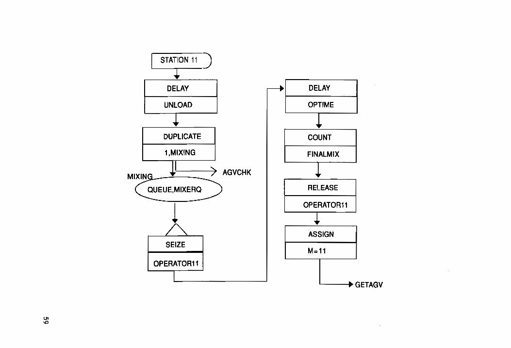
'----------t-- )
DELAY r DELAY
UNLOAD OPTIME
DUPLICATE I COUNT
1 ,MIXING FINALMIX
~ ) AGVCHK
RELEASE
OPERATOR11
ASSIGN SEIZE
M=11
OPERATOR11
L--____ GETAGV

(J'\ o
STATION 12) ,
DELAY
UNLOAD
~ DUPLICATE
1 ,BLOCKER
~ ) AGVCHK BLOCKE
~'BLO~
~ SEIZE
OPERATOR12
I
... DELAY -,.
OPTIME
r RELEASE
OPERATOR11
LGE TAGV
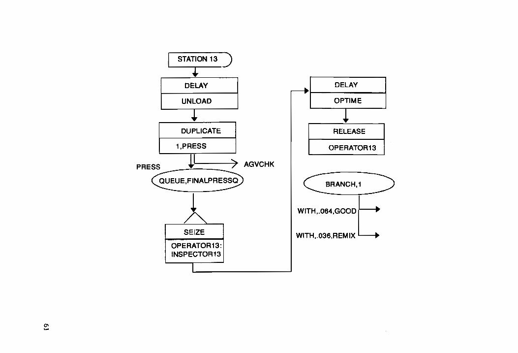
STATION 13 )
+ DELAY DELAY
UNLOAD OPTIME
DUPLICATE RELEASE
1,PRESS OPERATOR13
PRESS ~ ) AGVCHK
1 ~ SEIZE
L. WITH,.064,GOOD L WITH,.036,REMIX
OPERATOR13: INSPECTOR13
0"0 .......
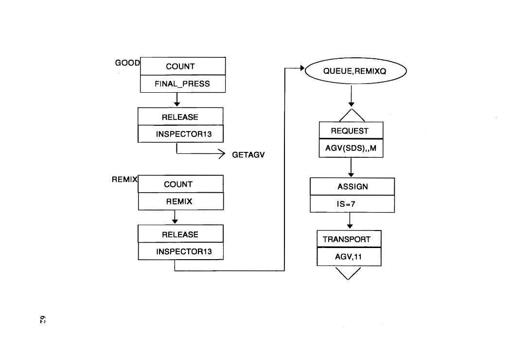
0\ t,
GOO -
REMIX r ..
COUNT
FINAL_PRESS
~ RELEASE
INSPECTOR13
I
COUNT
REMIX
~ RELEASE
INSPECTOR13
I
.. ,..
) GETAGV
1 REQUEST
AGV(SDS)"M
1 ASSIGN
IS=7
~ TRANSPORT
AGV,11
""/
~ (.oJ
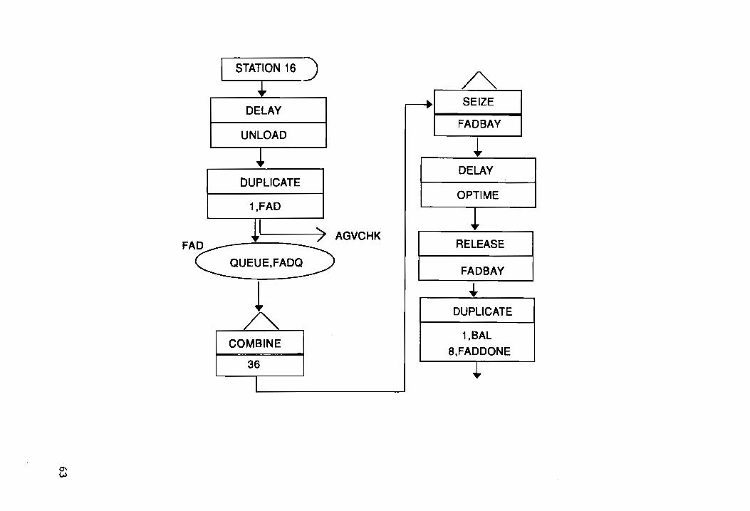
STATION 16 )
DELAY
UNLOAD
DUPLICATE
1,FAD
• ') AGVCHK
COMBINE
36
. .
I I
/ r"1
SEIZE
FADBAY
J DELAY
OPTIME
+ RELEASE
FADBAY
• DUPLICATE
1,BAL
8,FADDONE
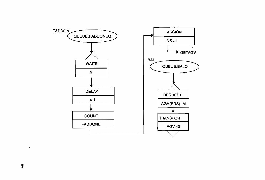
Q\ ~
WAITE
2
DELAY
0.1
COUNT
FADDONE
ASSIGN
NS=1
--------. GETAGV
REQUEST
AGV(SDS)"M
TRANSPORT
AGV,40
/
...... w ~ (!) a: w I- ~ 0 ~
e w ::E z w ~ ~ -' t- ::> ~ --+~ w a: w a.. 0 w Ul w e 0 (.) Ul z a..
0
i ~ :J: (.)
> (!) c(
() I i'
w w 0
"" ~ ~ II ,... e -'
z ~ c( () ~ () z c(
0 0 -' :J (!) z !;t r-+ .-J
-' ~ D.. ~ 1-. Q.. ..... Ul (!) W I-e z ::> ~ ::> C')
.. Ul Ul ~ :::J C 0 c( ~ en
c(
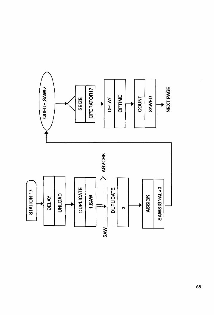
----- ((J
65
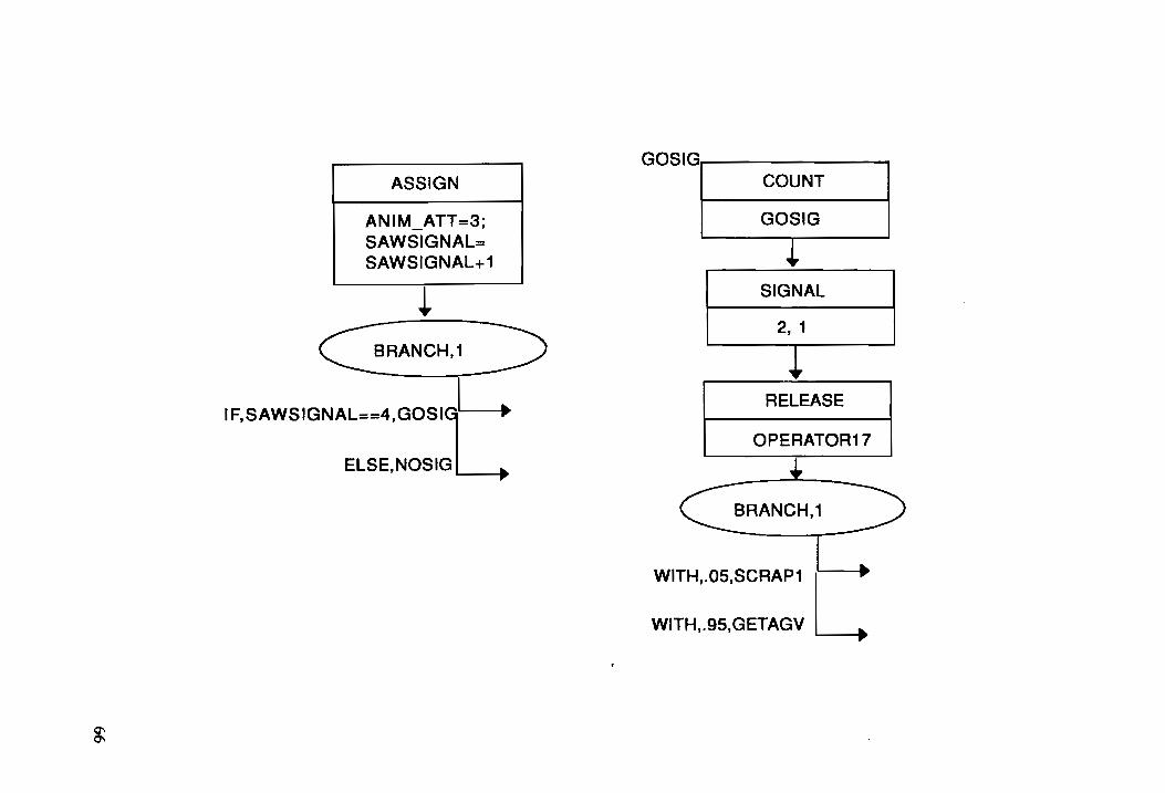
~
ASSIGN
ANIM_ATT=3; SAWSIGNAL= SAWSIGNAL+1
~
IF,SAWSIGNAL==4,GOSj :
ELSE,NOSIG
GOSIG COUNT
GOSIG
~ SIGNAL
2, 1
~ RELEASE
OPERATOR17
+ BRANCH,1
WITH,.05,SCRAP1 II :
WITH,.95,GETAGV

(!)
en o z
67

'" (»
SCRAP1 COUNT
SCRAP1
~ ASSIGN
ANIM_ATT=5
REQUEST
AGV(SDS)"M
TRANSPORT
AGV,38
'V

DELAY DELAY RELEASE
UNLOAD OPTIME INSPECTOR18
DUPLICATE RELEASE COUNT
1,MACHINE OPERATOR18 MACHINE
MACHINE AGVCHK
BRANCH.1
ITH •. 03,SCRAP
SEIZE SEIZE
INSPECTOR18 WITH .. 97.GETAGV· •
OPERATOR18
$
" o
DELAY
UNLOAD
~ DUPLICATE
1 ,LABEL
I ......... /'
FOR NEXT 3 STATIONS: 19 GRAIN PREP 20 INSERT PIN 21 CURE2
~, -LABE_
~UE.STATIO~ UEUE,STATION(
- -
SEIZE
OPERATOR
GETAGV
.....,
.....
XRAY
DELAY
UNLOAD
DUPLICATE
1,XRAY
..J.: ) AGVCHK
SEIZE
OPERATOR22
DELAY
OPTIME
RELEASE
OPERATOR22
COUNT
XRAY
BRANCH,1
WITH •. 15.S0RAP1 C WITH, .85,GETAGV
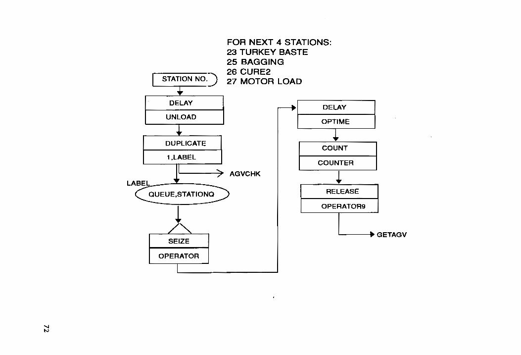
'" l'-.)
DELAY
UNLOAD
DUPLICATE
1 ,LABEL
~ SEIZE
OPERATOR
FOR NEXT 4 STATIONS: 23 TU RKEY BASTE 25 BAGGING 26 CURE2 27 MOTOR LOAD
DELAY
OPTIME
COUNT
COUNTER
AGVCHK ~ RELEASE
OPERATOR9
'-----... GETAGV
........ w
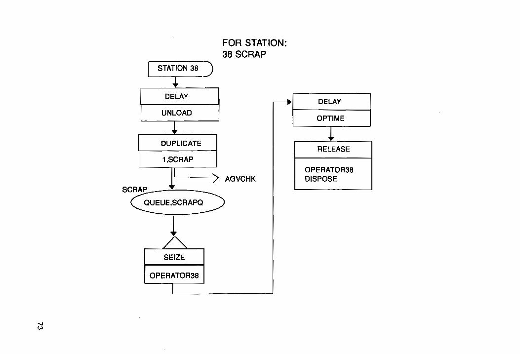
FOR STATION: 38 SCRAP
STATION 38 ) j
DELAY
UNLOAD
+ DUPLICATE
1,SCRAP J
) AGVCHK l -
SCRAP
~E.SCRAV
1 SEIZE
OPERATOR38
l
JIll" DELAY
OPTIME
1 RELEASE
OPERATOR38 DISPOSE
...., ~
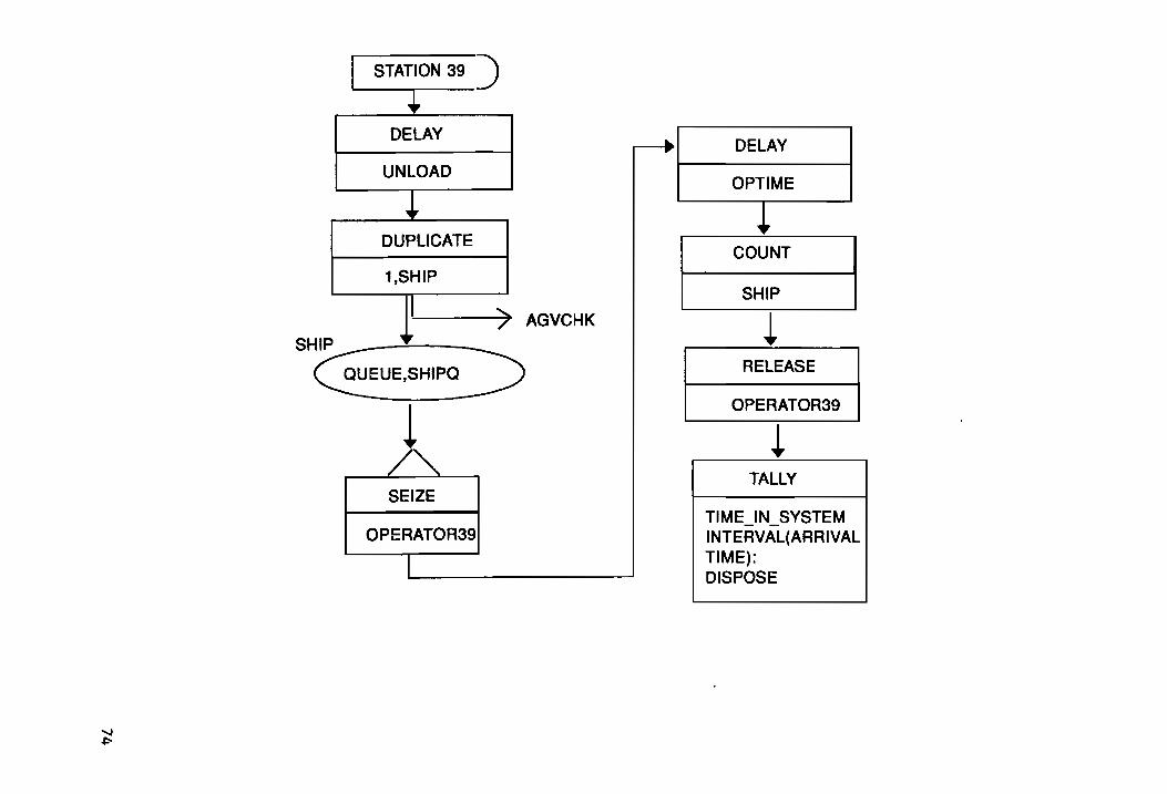
STATION 39 ) ,
DELAY
UNLOAD
~ DUPLICATE
1,SHIP
) AGVCHK l -
SHIP
~UE.SH'P0
1 SEIZE
OPERATOR39
I
.... ... DELAY
OPTIME
~
I
COUNT
SHIP
~ RELEASE
OPERATOR39
~ TALLY
TIME -INTER L TIME): DISPO S
...... c.n
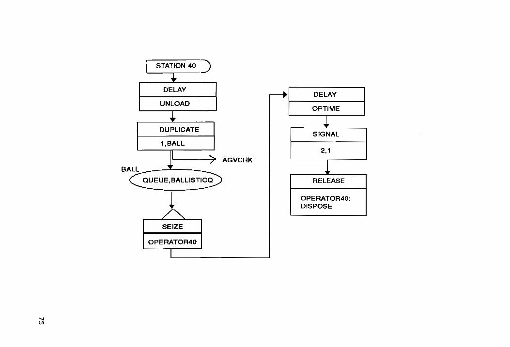
BALL
DELAY
UNLOAD .., DUPLICATE
1.BALL
~ =: ---QUEUE,BALLISTICa
--- .----'
SEIZE
OPERATOR40
> CJ <C w CJ i5 en
I-z :::J 0 0
0 w (!)
~ en
,.-
w ~ f--+ > m
0 (!) -+
::E <
n ,.- w .q- en z w .. ~ 0 r-+ w >en ~ a: (!)-l- LL. <0 en
i....-.
W CJ i5 en 0 z
76

Appendix III
77
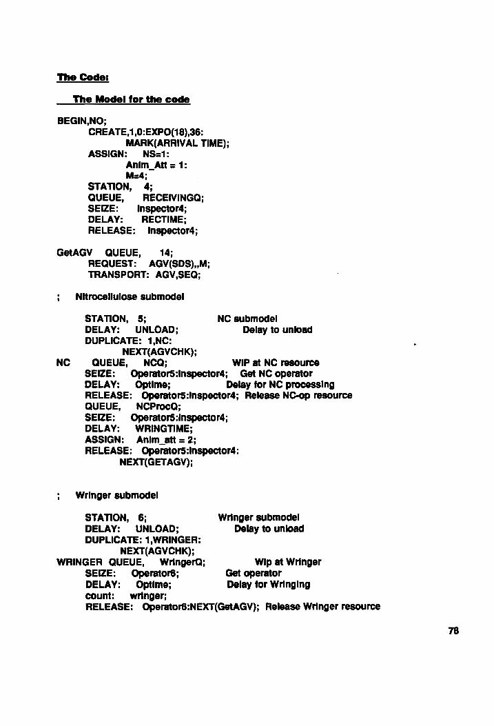
The Code:
The Model for the code
BEGIN,NO; CREATE,1,O:EXPO(18),36:
MARK(ARRIVAL TIME); ASSIGN: NS=1:
Anlm_Att = 1: M=4;
STATION, 4; QUEUE, RECEIVINGQ; SEIZE: Inspector4; DELAY: RECTIME; RELEASE: Inspector4;
GetAGV QUEUE, 14; REQUEST: AGV(SDS)"M; TRANSPORT: AGV,SEQ;
Nitrocellulose submode'
STATION, 5; NC submodel DELAY: UNLOAD; Delay to unload DUPLICATE: 1,NC:
NEXT(AGVCHK); NC QUEUE, NCQ; WlP at NC resource
SEIZE: Operator5:lnspector4; Get NC operator DELAY: Optlme; Delay for NC processing RELEASE: Operator5:lnspector4; Release NC-OP resource QUEUE, NCProcQ; SEIZE: Operator5:lnspector4; DELAY: WRINGTlME; ASSIGN: Anlm_Btt = 2; RELEASE: Operator5:lnspector4:
NEXT(GET AGV);
Wringer submodel
STATION, 6; DELAY: UNLOAD; DUPLICATE: 1.WRINGER:
NEXT(AGVCHK); WRINGER QUEUE, WringerQ;
SEIZE: Operator6; DELAY: Optlme; count: wringer;
Wringer sublnodel Delay to unload
Wlp at Wringer Get operator Delay for Wringing
RELEASE: Operator6:NEXT(GetAGV); Release Wringer resource
78
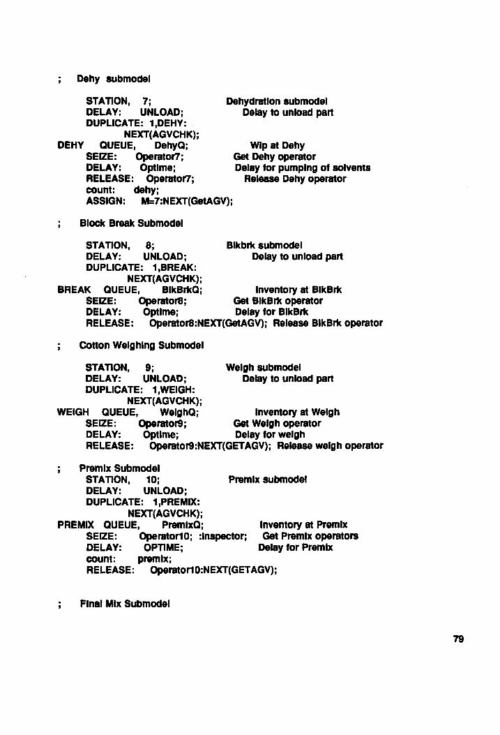
Dehy 8ubmodel
STATION, 7; DELAY: UNLOAD; DUPLICATE: 1,DEHY:
NEXT(AGVCHK); DEHY QUEUE, DehyQ;
SEIZE: Operator7; DELAY: Optlme; RELEASE: Operator7; count: dehy;
Dehydration submodel Delay to unload pan
Wlp at Dehy Get Dehy operator Delay for pumping of solvents
Release Dehy operator
ASSIGN: M=7:NEXT(GetAGV);
Block Break Submodel
STATION, 8; Blkbrk submodel DELAY: UNLOAD; Delay to unload pan DUPLICATE: 1,BREAK:
NEXT(AGVCHK); BREAK QUEUE, BlkBrkQ; Inventory at BlkBrk
SEIZE: OperatorS; Get BlkBrk operator DELAY: Optlme; Delay for BlkBrk RELEASE: OperatorS:NEXT(GetAGV); Release BlkBrk operator
Cotton Weighing Submodel
STATION, 9; Weigh submodel DELAY: UNLOAD; Delay to unload pan DUPLICATE: 1,WEIGH:
NEXT(AGVCHK); WEIGH QUEUE, WelghQ; Inventory at Weigh
SEIZE: Operator9; Get Weigh operator DELAY: Optlme; Delay for weigh RELEASE: Operator9:NEXT(GETAGV); Release weigh operator
Premix Sub model STATION, 10; Premix submodel DELAY: UNLOAD; DUPLICATE: 1,PREMIX:
NEXT(AGVCHK); PREMIX QUEUE, PremlxQ; Inventory at Premix
SEIZE: Operat0r10; :Inspector; Get Premix operators DELAY: OPTIME; Delay for Premix count: premix; RELEASE: Operat0r10:NEXT(GETAGV);
Final Mix Submodel
79
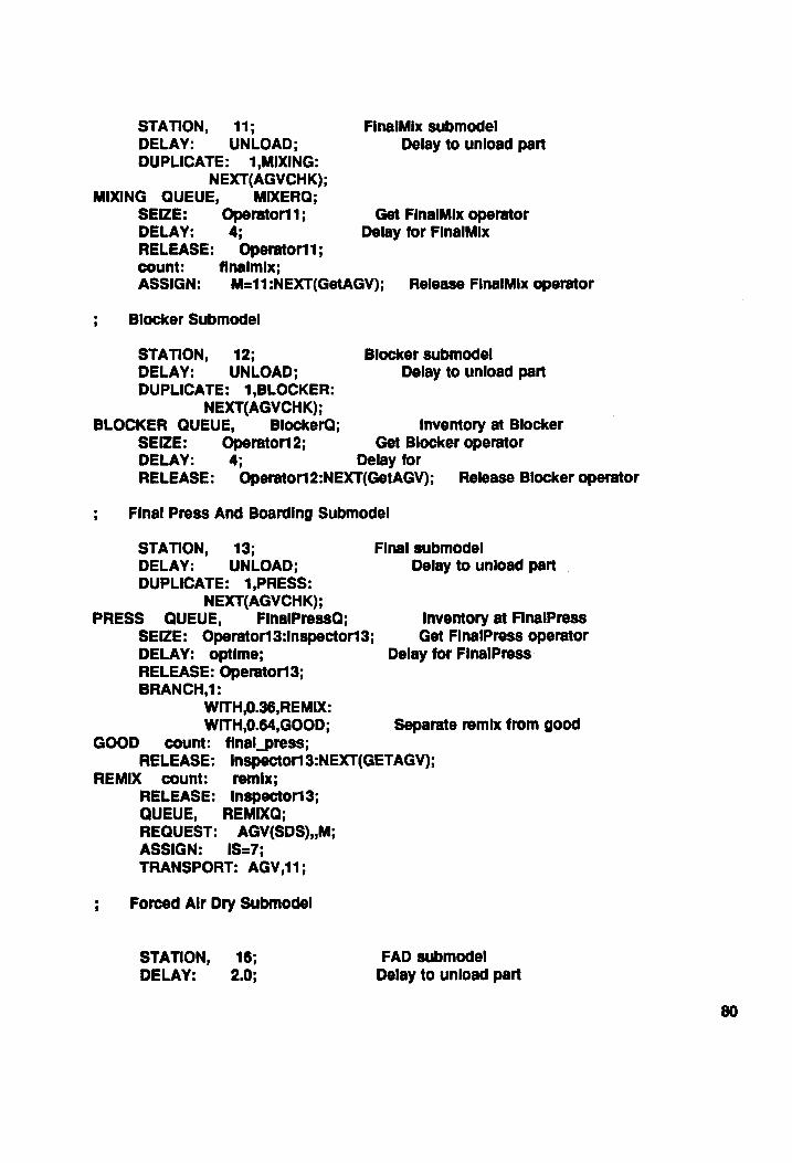
STA nON, 11; FlnelMlx submodel DELAY: UNLOAD; Delay to unload pan DUPLICATE: 1,MIXING:
NEXT(AGVCHK); MIXING QUEUE, MIXERQ;
SEIZE: Operat0r11; Get FlnalMlx operator DELAY: 4: Delay for FlnalMlx RELEASE: Operat0r11 ; count: ftnalmlx; ASSIGN: M=11 :NEXT(GetAGV); Release FlnalMlx operator
Blocker Submodel
STAn ON , 12; Blocker submodel DELAY: UNLOAD: Delay to unload pan DUPLICATE: 1,BLOCKER:
NEXT(AGVCHK); BLOCKER QUEUE, BlockerQ; Inventory at Blocker
SEIZE: Operator12; Get Blocker operator DELAY: 4; Delay for RELEASE: Operator12:NEXT(GetAGV): Release Blocker operator
Final Press And Boarding Submodel
STAnON, 13: DELAY: UNLOAD; DUPLICATE: 1,PRESS:
NEXT(AGVCHK); PRESS QUEUE, FlnalPressQ;
SEIZE: Operator13:lnspector13; DELAY: optlme; RELEASE: Operator13: BRANCH,1:
WITH,O.38,REMIX: WITH,O.64,GOOD;
GOOD count: flnal...press;
Final submodel Delay to unload pan
Inventory at FlnalPress Get FlnalPress operator
Delay for FlnalPress
Separate remix from good
RELEASE: Inspector13:NEXT(GETAGV); REMIX count: remix;
RELEASE: Inspector13: QUEUE, REMIXQ; REQUEST: AGV(SDS)nM; ASSIGN: IS=7; TRANSPORT: AGV, 11 ;
Forced Air Dry Submodel
STATION, 16; DELAY: 2.0;
FAD submodel Delay to unload pan
80
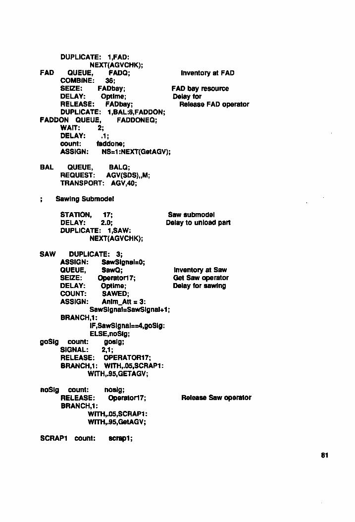
DUPLICATE: 1,FAD: NEXT(AGVCHK);
FAD QUEUE, FADQ; COMBINE: 36: SEIZE: FADbay; DELAY: Optlme; RELEASE: FADbaYi DUPLICATE: 1,BAL:8,FADDON;
FADDON QUEUE, FADDONEQ; WAIT: 2; DELAY: .1; count: faddone; ASSIGN: NS=1 :NEXT(GetAGV);
BAL QUEUE, BALQ; REQUEST: AGV(SDS)"M; TRANSPORT: AGV,40;
Sawing Submodel
Inventory at FAD
FAD bay resource Delay for
Release FAD operator
STATION, 17: DELAY: 2.0;
Saw 8ubmodel Delay to unload pan
DUPLICATE: 1,SAW: NEXT(AGVCHK);
SAW DUPLICATE: 3; ASSIGN: SawSlgnal=O; QUEUE, SawQ: SEIZE: Operat0r17; DELAY: Optlme; COUNT: SAWED; ASSIGN: Anlm_AH = 3:
SawSlgnal=SawSlgnal+ 1 ; BRANCH,1:
IF ,SlwSlgnal==4,goSlg: ELSE,noSlg;
goSlg count: goslg; SIGNAL: 2,1 ; RELEASE: OPERATOR17; BRANCH,1: WITH,.05,SCRAP1:
WITH,.95,GETAGV;
noSlg count: noslg; RELEASE: Operat0r17; BRANCH,1:
WITH,.05,SCRAP1 : WrrH,.95,GetAGV;
SCRAP1 count: scrap1 ;
Inventory at Saw Get Saw operator Delay for sawing
Release Saw operator
81
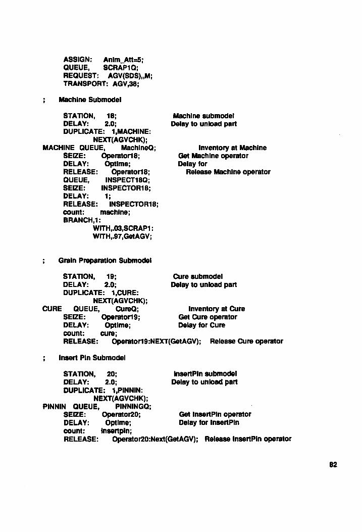
ASSIGN: Anlm_Att=5; QUEUE, SCRAP1Q; REQUEST: AGV(SDS)"M; TRANSPORT: AGV,38;
Machine Submodel
STAn ON , 18; DELAY: 2.0; DUPLICATE: 1,MACHINE:
NEXT(AGVCHK); MACHINE QUEUE, MachlneQ;
SEIZE: Operat0r18; DELAY: Optlme; RELEASE: Operator18; QUEUE, INSPECT18Q; SEIZE: INSPECTOR18; DELAY: 1; RELEASE: INSPECTOR18; count: machine; BRANCH,1:
WITH,.03,SCRAP1 : WITH, .. 97,GetAGV;
Grain Preparation Submodel
STAnON, 19; DELAY: 2 .. 0; DUPLICATE: 1,CURE:
NEXT(AGVCHK); CURE QUEUE, CureQ;
SEIZE: Operat0r19; DELAY: Optlme: count: cure;
Machine sub model Delay to unload pan
Inventory at Machine Get Machine operator Delay for
Release Machine operator
CUre submodel Delay to unload pan
Inventory at CUre Get Cure operator Delay for Cure
RELEASE: Operator19:NEXT(GetAGV): Release Cure operator
Insert Pin Submodel
STA nON, 20; InsenPln submodel DELAY: 2.0: Delay to unload pan DUPLICATE: 1,PINNIN:
NEXT(AGVCHK); PINNIN QUEUE, PINNINGQ;
SEIZE: Operator20; Get InsenPln operator DELAY: Optlme; Delay for InsenPln count: Inaenplnj RELEASE: Operator20:Next{GetAGV); Release InsertPln operator
82
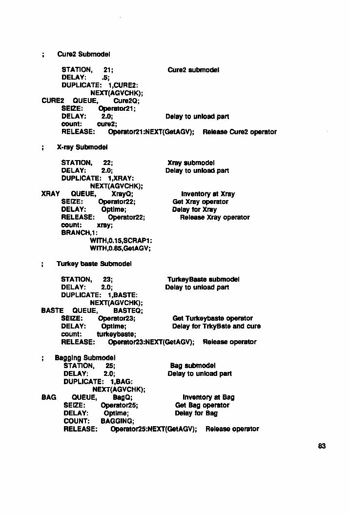
CUre2 Submodel
STATION, 21; CUre2 submodel DELAY: .5; DUPLICATE: 1,CURE2:
NEXT(AGVCHK); CURE2 QUEUE, CUre2Q;
SEIZE: Operator21 ; DELAY: 2.0; Delay to unload pan count: cure2; RELEASE: Operator21 :NEXT(GetAGV); Release CUre2 operator
X-ray Submodel
STATION, 22; DELAY: 2.0: DUPLICATE: 1 ,XRAY:
NEXT(AGVCHK);
Xray submodel Delay to unload pan
XRAY QUEUE, XrayQ; Inventory at Xray Get Xray operator Delay for Xray
SEIZE: Operator22; DELAY: Optlme; RELEASE: Operat0r22; Release Xray operator count: xray; BRANCH,1:
WITH,0.15,SCRAP1 : WITH,O.85,GetAGV;
Turkey baste Submodel
STATION, 23; TurkeyBaste submodel DELAY: 2.0j Delay to unload pan DUPLICATE: 1 ,BASTE:
NEXT(AGVCHK); BASTE QUEUE, BASTEQ;
SEIZE: Operator23; Get Turkeybaste operator DELAY: Optlme; Delay for TrkyBste and cure count: turkeybaste; RELEASE: Operator23:NEXT(GetAGV}; Release operator
Bagging Submodel
BAG
STATION, 25; DELAY: 2.0; DUPLICATE: 1.BAG:
NEXT(AGVCHK); QUEUE, BagQ;
SEIZE: Operator25; DELAY: Optlme; COUNT: BAGGING;
Bag submodel Delay to unload pan
Inventory at Bag Get Bag operator Delay for Bag
RELEASE: Operator25:NEXT(GetAGV); Release operator
83
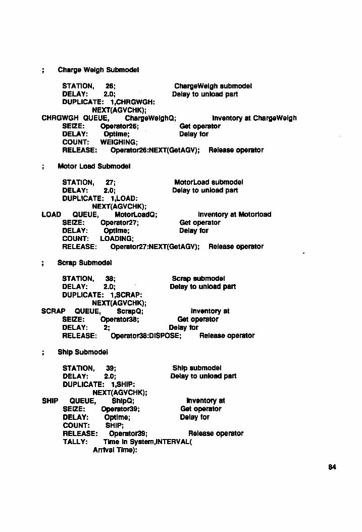
Charge Weigh Submodel
STAnON, 28; CbargeWelgh submodel DELAY: 2.0; Delay to unload pan DUPLICATE: 1,CHRGWGH:
NEXT(AGVCHK); CHRGWGH QUEUE, CbargeWelghQ; Inyentory at CbargeWelgh
SEIZE: Operator28: Get operator DELAY: Optlme; Delay tor COUNT: WEIGHING; RELEASE: Operator28:NEXT(GetAGV); Release operator
Motor Load Submodel
STAn ON , 27: DELAY: 2.0; DUPLICATE: 1 ,LOAD:
NEXT(AGVCHK); LOAD QUEUE, MotorLoadQ;
SEIZE: Operator27; DELAY: Optlme; COUNT: LOADING;
MotorLoad submodel Delay to unload pan
Inventory at Motorload Get operator Delay for
RELEASE: Operator27:NEXT(GetAGV); Release operator
Scrap Submodel
STATION, 38; Scrap submociel DELAY: 2.0: Delay to unload pan DUPLICATE: 1 ,SCRAP:
NEXT(AGVCHK); SCRAP QUEUE, ScrapQ; Inventory at
SEIZE: OperatOr38; Get operator DELAY: 2; Delay tor RELEASE: Operator38:DISPOSE; Release operator
Ship Submodel
STATION, 39; DELAY: 2.0; DUPLICATE: 1,SHIP:
NEXT(AGVCHK); SHIP QUEUE, ShlpQ;
SEIZE: Operator39; DELAY: Optlme: COUNT: SHIP;
Ship submodel Delay to unload pan
In~entory at Get operator Delay for
RELEASE: Operator39; Release operator TALLY: Time In System,INTERVAL(
Arrtval Time):
84
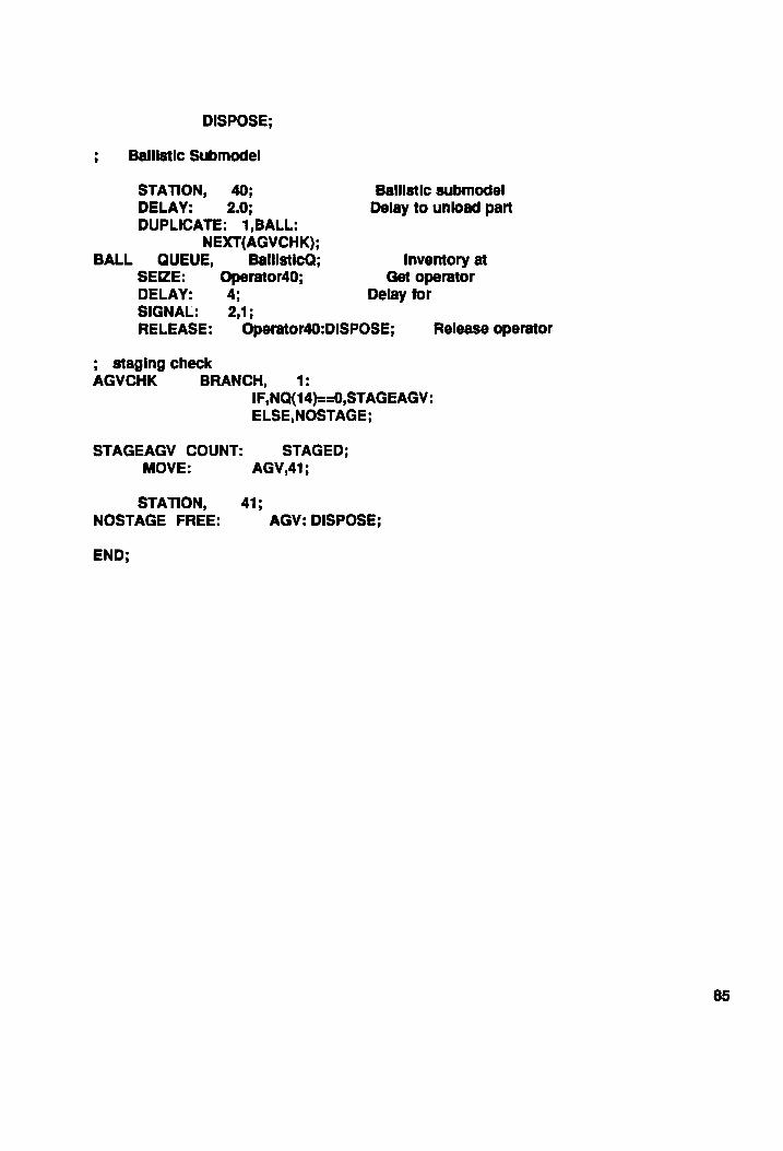
DISPOSE;
Ballistic Sub model
STATION, 40; DELAY: 2.0; DUPLICATE: 1 ,BALL:
NEXT(AGVCHK); BALL QUEUE, BalllstlcQ;
SEIZE: Operator40; DELAY: 4; SIGNAL: 2,1;
Ballistic submodel Delay to unload pan
Inventory at Get operator
Delay for
RELEASE: Operator40:DISPOSE; Release operator
staging check AGVCHK BRANCH, 1 :
IF,NQ(14)=::O,STAGEAGV: ELSE,NOSTAGE;
STAGEAGV COUNT: STAGED; MOVE: AGV,41;
STATION, 41; NOSTAGE FREE: AGV: DISPOSE;
END;
85

Appendix IV
86
The experiment for the code
jSIMULATION OF THE TOW LAUNCH PROPELLANT MANUFACTURING PROCESS AT RAAP ;FINAL PROJECT ;DAN A. CREMER BEGIN,no,no; PROJECT, TOW LAUNCH MFG PROCESS,DanC; ATTRIBUTES: Amva' Time:
OpTlme: Anlm_Att: 4;
VARIABLES: SawSlgnal: COTTONSIZE,72:RECTIME,4.0: UNLOAD,1 :WRINGTlME,6: BATCHSIZE,72:REWORK,O.20:HPCSIZE,72: SUBLOTS,3:SAWSCRAP,O.10:MACHSCRAP,O.05: XRAYSCRAP,O.20;
QUEUES: 4,RECEIVINGQ:5,NCQ:6,WRINGERQ:7,DEHYQ:S,BLKBRKQ:9,WEIGHQ: 10,PREMIXQ:11,FINALMIXQ:12,BLOCKERQ:13,FINALPRESSQ: 14,loadq:16,FADQ:17,SAWQ:1S,MACHINEQ: 19,CUREQ:20,INSERTPINQ:21 ,CURE2Q:22,xRAYQ:23,TURKEYBASTEQ: 26,CHARGEWEIGHQ:27,MOTORLOADQ:2S,IBLQ: 29,PINSQ:30,COMPONENTPREPQ:31,IGNITERQ:32,FINALPACKQ: 33,SYRUPPREPQ:34,SOLVENTSQ:35,NGQ:36,CHEMICALSQ: 37 ,CHEMLABQ:38,SCRAPQ:39,SHIPQ:40,BALLISTlCQ: COTTONQ:NEATNGQ:LABQ:POACHERQ:NCRESULTSQ:NCPRODQ: NCPROCQ:PREMIXPROCQ:LabOutQ:MIXINGQ:REMIXQ:SOLVENQ: MIXERQ:AGUQ:WRINGQ:DEHYDQ:DHDATAQ:DHDONEQ:CHEMSQ: FADDONEQ:BALQ:INSPECT1SQ:CHEMDONEQ:SCRAP1 Q:DHTRNQ: PlnsReadyQ:SyrupreadyQ:CUre2done:BasteQ:PlnnlngQ: BagQ:SYRUPREADY1Qj
RESOURCES: Inspector(5):lnspector4(1 ):lnspector1 0(6): Inspect0r13(3):lnspect0r17{1):lnspectonS(1): Inspect0r22(6):lnspector27(5) :lnspector28(5): Inspect0r32(6):lnspect0r37(5):lnspector40(6): PRESSeS): Operat0r5(1):Operator6(1):Operat0r7(1):Operator8(1): Operator9(1 ): Operaton O(2):Operaton1 (1 ):Operat0r12(1): Operaton3(3): FADBay(2),74:Operator17(1) : Operat0r1S(1 ): Operaton9(1 ):Operator20(1) :Operator21 (1): Operat0r22(1 ): Operat0r23(1 ):Operator25(1 ),6:
87
Operator26(1 ): Operator27(1 },4:0perator28(1) :Operator29(1): Operator30(1 }: Operator31 (1 ):Operator32(1 ) :Operator33(1): Operat0r34{1 ): Operator35(5):Operator38(1 ):Operator37(1): Operator38(1 ),4: Operator39(1 ),4:Operator4O(1);
STATIONS: 4" 1 :5,,6:6,,9:7,,29 :8,,2:9,,19:10,,45:11,,15:12,,16: 13,,5:15,,8:16,,47:17,,35:18,,40:19,,41 :20,,42:21 ,,42: 22,,22:23,,42:25,,37:26,,43:27,,43:28,,23:29,,37: 30,,37:31,,37:32,,43:33,,42:34.,27:35,,45:36,.28:37,,26: 38,,31 :39,,30:40,,46:41 ,stage,48:42" 15:43"29:44,, 11:
SEQUENCES: 1, 5,Optlme=LOGN(4,.2) & 6,Optlme=LOGN(4,.2). 7,Optlme:LOGN(4,.2). 8,Optlme=LOGN(4,.2) • 9,Optlme:LOGN(5,.2) &
10,OpUme=LOGN(4,.2). 11,Optlme=LOGN(4,.2). 12,Optlme:LOGN(3,.1) & 13,Optlme:LOGN(5,.2) & 16,Optlme::LOGN(10,.2) & 17,Optlme:LOGN(4,.2) & 18,Optlma::LOGN(8,.2) & 19,Optlma::LOGN(8,.31) & 2O,Optlme:LOGN{2,.1) • 21,Optlme=LOGN(4,.2) & 22,Optlme=LOGN{2,.1) & 23,Optlme:LOGN(8,.2) & 25,Optlme:LOGN(3,.1) & 26,Optlma::LOGN(2,.1) & 27,Optlme:LOGN(2,.1) & 39,Optlme::LOGN(2,.1 );
STORAGES: FADSTR: RECEIVING;
COUNTERS: WRINGER:DEHV:PREMIX:FINALMIX:FINAL_PRESS:REMIX: FADDONE:GOSIG:NOSIG:SCRAP1 :SAWED:MACHINE:CURE:INSERTPIN: CURE2:XRAV:TURKEVBASTE:BAGGING:WEIGHING: LOADING:SHIP:STAGED;
INTERSECTIONS: 1,:2,:3,:4,:5,:6,:7,:9,:11,:13,:15,:16,:17,:18,: 19,:20,:21,:22,:23,:24,:25,:26,:27,:28,:29,:30,: 31,:32,:33,:34,:35,:36,:37,:38,:39,:40,:41,:42,: 43, :44,:45, :46, :47,:48,;
LINKS: 1,,3,1,10,1o,Spur: 2,,3,6,8,10:3.,6,3,8,10:4,,3,13,5,10:5,,13,3,5,10: 6,,6,9,6,10:7,,9,6,6,10:8 .. 9,3,1,60: 9,,3,9,1,80:10,,9,29,1,50:11,,29,9,1,50:
12,,13,29,1,100:13,,29,13,3,100: 14,,29,28,2,35,SPUR: 15" 13,7,10,5:16,,7,13,10,5 :17,,7,5,1,120:18,,5,7,1,120: 19,,5,27,7,10,SPUR: 20,,5,14,1 ,50:21" 14,5, 1,50 :22" 14,15,1,50:23., 15,14,1,50:
88
24" 15, 11,1,50:25" 11,15,1,50:26,,11,16,1,60: 27" 16, 11, 1,60:28" 16, 17,1,50:29,,17,16,1,50: 30"4,17,1,10:31,, 17,4,1,10: 32,,4,2,3,3 : 33,. 18,4, 1,50:34,,4,18,1,50: 35" 18, 19, 1,65:36,,19,18,1,65: 37,,19,20,1,15:38,,20,19,1,15: 39" 18,20, 1,70:40.,20,18,1,70: 41,,20,21,2,45:42,,21,20,2,45: 43,,21,22,1,75,SPUR: 44,,21,24,1,50:45,,24,21,1,50: 46,,24,25,1,10: 47,,25,26,1 ,70,S PUR: 48,,25,23,2,45: 49 ,,23,24,2,50: SO" 18,32, 10,50:51,,32,18,10,50: 52,,32,30,2,5: 53,,32,31,10,50:54,,31,32,10,50: 55,,32,33,10,80:56,,33,32,10,60: 57,,33,34,1,10:60,,34,33,1,10: 61,,34,35,6,10:62,,35,34,6,10: 63,,33,36,5,10:64,,36,33,5,10: 65,,36,37,1,1 OO,SPUR: 86,,36,38,10,10:67,,38,36,10,10: 68,,38,39,2,50 :69 .. 39,38,2,50: 70,.38,43,5,15:71,,43,38,5,15: 72,,43,42,5,15:73,,42,43,5,15: 74,,42,41,2,10:75,,41,42,2,10: 78,,41,40,1,15:77.,40,41,1 f 15: 78,,40,39,3,10:79,,39,40,3,10: 80,,41,39,3,11 :81,,39,41,3,11 : 82,,39,44,10,10:83,.44,39,10,10: 84,,44,47,3,8: 85,,44,45,10,10:86,,45,44,10,10: 87 ,,45,46, 15, 10:88,,46,45,15,10: 89,,46,44,15,10:90,,44,46,15,10: 91,,24,48,15,5: 92,LINK92,48,21 ,15,5:93" 17,14,1,50: 94" 14, 17,1,50:95,,2,4,3,3:96,,47,44,3,6: 97,,30,32,2,5:98,,33,30,10,80;
NETWORKS: 1,AGV System,1-98;
TRANSPORTERS: 1 ,AGV,2,NETWORK(AGV System), 5380.0,LINK(92) ;
TALLIES: nme In System;
DSTATS: NQ(14),AGV QUEUE:
89
NQ(NCQ),NC QUEUE: NQ{NCPROCQ}: NQ(wrlngerq},WRINGER QUEUE: NQ(dehyq),DEHY QUEUE: NQ{BLKBRKQ),BLOCK BREAK QUEUE: NQ(WEIGHQ), WEIGH QUEUE: NQ(PREMIXQ),PREMIX QUEUE: NQ{FINALMIXQ},FINAL MIX QUEUE: NQ(BLOCKERQ),BLOCKER QUEUE: NQ(FINALPRESSQ),FINAL PRESS QUEUE: NQ{REMIXQ),REMIX QUEUE: NQ(FADQ),FAD QUEUE:NQ(FADDONEQ),FAD DONE QUEUE: NQ(SAWQ): NQ(MACHINEQ):NQ(INSPECT18Q),MACHINE INSP .Q: NQ(CUREQ),GRAIN PREP QUEUE: NQ(PINNINGQ): NQ{CURE2Q): NQ{CURE2DONE): NQ(XRAYQ): NQ(BASTEQ):NQ(BAGQ):NQ(CHARGEWEIGHQ): NQ(MOTORLOADQ):NQ(SHIPQ):
IT(AGV,1},AGV 1 Time Active: IT(AGV,2),AGV 2 Time Active: IT(AGV,3),AGV 3 Time Active: IT(AGV,4),AGV 4 Time Active: IT(AGV,5),AGV 5 Time Active:
IT(AGV,6),AGV 6 Time Active: IT(AGV,7),AGV 7 Time Active:
MAX(NT(1 }-NL(LINK92),O)l5,AGV Actual Busy:
IT(AGV,8): ITCAGV,9): IT(AGV,10}: JT(AGV,11): IT(AGV,12): IT(AGV,13): IT{AGV,14): ITCAGV,15):
NR(INSPECTOR4),RECEIVING STATION: NR(OPERATOR5),NITROCOTTON STATION: NR(OPERATOR6),WRINGER STATION: NR(OPERATOR7),DEHYS: NR(OPERATOR8),BLOCKBREAKS:NR(OPERATOR9),WEIGHS: NR(OPERATOR10),PREMIX STATION: NR(OPERATOR11),FINAL MIX STATION:
90
NR(OPERATOR12),BLOCKERS: NR(OPERATOR13),PRESS AND BOARD: NR(FADBAy),FAD BAY:NR(OPERATOR17),SAW STATION: NR(INSPECTOR17),SAW INSPECTION: NR(OPERATOR18),MACHINING STATION: NR(INSPECTOR18),MACHINING: NR(OPERATOR19},GRAIN PREP: NR(OPERAT0R20),PINNING STATION: NR(OPERATOR21 ),CURING BAY:NR(OPERA TOR22},xRA Y STATION: NR(OPERATOR23),TURKEYBASTING: NR{OPERATOR25),BAGGING STAnON: NR(OPERATOR26),CHRG WEIGHING: NR(OPERATOR27),MOTOR LOADING: NR(OPERATOR39),SHIPPING: NR(OPERATOR38),BURNING GROUNDS;
LAYOUTS: "PROJ.LA Y" ,Anlm_Att,.1; REPLICATE, 2,0,2880, YES, YES,O.O; END;
91

Appendix V
92

S~ xv - L1a~e '9110443 Vlrgi:Aia ftah.
su..ar.v for -.pliaatiOD 1 of 20
Projeat, IJ'OW LA.tJIICB IIPG PllOCBSS JlUD ezec:nltiOD date , 1/25/1993 ADalyata DaD.C IIo4el reYiaiOD date. 1/24/1993
BeplicatiOD tmele4 at tt- I 2880.0
X4eDtifier Average VariatiOD Ki:a!.a. lla:l:bua ObaervatiODa
-.rt.. III 8yatea 345.18 .23632 186.41 464.83 25
J)XBCU'l'B-CIIUIGB V'AJll:A.BLBS
Xdentifier Average Variat10D "h:I~.I. "z:l_lm .. iDal Value
'AtJV QUB'O'B .04185 6.1169 .00000 4.0000 .00000 He QUB'O'B .09145 5.7636 .00000 6.0000 .00000 IJQ (IlCPROCQ) .14054 4.5646 .00000 6.0000 .00000 1fR.D1'CDR QUBUB .00000 .00000 .00000 .00000 JDBY Q'OBtJI: .91129B-06 1047.5 .00000 1.0000 .00000 BLOClt BIlBAJt QUB'O'B .24425B-03 63.978 .00000 1.0000 .00000 aXGB QtJ'B'OJI .71466B-03 37.393 .00000 1.0000 .00000 PlUDID QUBUB .00000 .00000 .00000 .00000 .%HAL lID QUJfO'B .00000 .00000 .00000 .00000 BLOCDIl Q17BtJB .00134 27.286 .00000 1.0000 .00000 "%HAL PUSS Qu:nB .547118-03 42.741 .00000 1.0000 .00000 UIID QtJ'B'OJI .22710B-03 66.351 .00000 1.0000 .00000 .Al) QUB'O'B 3.2413 2.3193 .00000 36.000 .00000 .Al) DO. Q1mlJJI .25202 4.7326 .00000 1.0000 .00000 IIQ (8.l.WQ) .07619 5.4429 .00000 3.0000 .00000 IIQ (IIACBDlBQ) .64215 3.6250 .00000 14.000 .00000 IACB%8B DlSP. Q .00000 .00000 .00000 .00000 CIItAD1 pup QUBUB .00933 10.302 .00000 1.0000 .00000 IfQ (PD1HD1OQ) .00000 .00000 .00000 .00000 IJQ (CUIUI2Q) .00000 .00000 .00000 .00000 IIQ (CURB2DO.) .00000 .00000 .00000 .00000 IIQ (:a::a&TQ ) .00000 .00000 .00000 .00000 IIQ(BASDQ) .00297 18.327 .00000 1.0000 .00000 IIQ(BAGQ) .00000 .00000 .00000 .00000 IfQ (CBA1\CJBRXGBQ) .00000 .00000 .00000 .00000 IIQ (JKm)l\LCW)Q) .00000 .00000 .00000 .00000 IIQ(SBXPQ) .00000 .00000 .00000 .00000 AIN 1 !'.iIDe Active .10185 .32989 .00000 1.0000 1.0000 ItDV 2 !'.iIDe Active .26415 1.6610 .00000 1.0000 .00000 AIN 3 !'.iIDe Active .11039 .31373 .00000 1.0000 1.0000 AIJV Actual hay .41421 .16161 .00000 .60000 .40000 DCB:tVD1Q H.I..,XOH .17456 2.1745 .00000 1.0000 .00000 lI:t'l'BOCO'l'.l"OH S'1'A'1'XOII .12456 2.6511 .00000 1.0000 .00000 WJtDIQ'IJl HAnOH .04974 4.3707 .00000 1.0000 .00000 marrs .04975 '.3706 .00000 1.0000 .00000 BLOCItB1UI.UUI .04915 '.3612 .00000 1.0000 .00000 DXGB8 .062'6 3.87'4 .00000 1.0000 .00000 pJlBlCDt 8'lA'1'XOH .04952 4.3809 .00000 1.0000 .00000 .%HAL IIlX S'1'A'1'XO& .08750 3.2293 .00000 1.0000 .00000 BLOCUikB .08750 3.2293 .00000 1.0000 .00000 PUB8 .um BOA1U) .08830 3.2133 .00000 1.0000 .00000 .Al)BAT .00353 16.793 .00000 1.0000 .00000 8.l.W SI'.I.'1'XO& .05079 4.3221 .00000 1.0000 .00000 aw D18PJICf1IXO& .00000 .00000 .00000 .00000 IACBDIDIG S'1'AnOIi .09725 3.0468 .00000 1.0000 .00000 IACBDJDIG .01215 1.0159 .00000 1.0000 .00000 CiIRAD' PUP .08818 3.2156 .00000 1.0000 .00000 P~ 8'1'A'1'XOII .02236 6.6117 .00000 1.0000 .00000
93

CtJaDIG BAY .02222 6.6333 .00000 1.0000 .00000 DAY STATXOR .02225 6.629' .00000 1.0000 .00000 '1'tJRD'!BA8TDtG .06963 3.6553 .00000 1.0000 .00000 BAGlGDtG 8'1'ATXOR .02609 6.1100 .00000 1.0000 .00000 CBRQ aXGBDIG .01732 7.531' .00000 1.0000 .00000 IIO'1'OR LOADDfG .01755 7.'822 .00000 1.0000 .00000 8BXPPDfG .01736 7.5238 .00000 1.0000 .00000 II1JIUID1G GROOlJDS .0076' 11.398 .00000 1.0000 .00000
COUII'1'DB
X4eD.tifier COWlt Liait
1lI.DJQBR 36 :Infinite J)DY 36 :Infinite PIUDClX 36 :Infinite I'lliIaLIaX 63 Xnfinite I'~P1UlSS 36 XDfinite BBIID[ 27 XAfinite I'ADDON'B 9 :InfiDJ.te QOSXG 9 :InfiDJ.te ROSXG 27 :Infinite 8CRAP1 11 :Infinite 8AWBD 36 :tDfinite IlACBDIB 35 :tDfiDJ.te CURB 32 XDfiDJ.te DDRTPD 32 XDfinit. CURB2 32 :InfiDJ.te DAY 32 :InfiDJ.t. ~ 25 :Infinite SBXP 25 XAfiDJ.te STAQBl) 576 XDfinit.
94

VITA
Dan A. Cremer was born on May 9, 1960 In Saigon, South Vietnam. He Immigrated to
the United States when he was nine years old. He attended Clarkson University, Potsdam,
New York and received his Bachelors of Science degree with a major In Industrial
Distribution In May of 1982.
After graduation, he worked for Texas Instruments for two years as a Manufacturing
Engineer for the F4 Radar Display Program. Then he worked for Simmonds Precision for
three years as the Manufacturing Engineer for the 81 B Fuel Management System. For the
last five years he has been working at the Radford Army Ammunition Plant as a Quality
Engineer.
Mr. Cremer began his graduate work In Industrial and Systems Engineering at Virginia
Polytechnic Institute and State University In January of 1991. He plans to stan a career with
Michelin Corporation February of 1993.
95