Angle of Incidence

And

Power Degradation Analysis of Photovoltaic Modules

by

Suryanarayana Vasantha Janakeeraman

A Thesis Presented in Partial Fulfillment of the Requirements for the Degree

Master of Science in Technology

Approved April 2013 by the Graduate Supervisory Committee:

Govindasamy Tamizhmani, Chair

Bradley Rogers Narciso Macia

ARIZONA STATE UNIVERSITY

May 2013

i

ABSTRACT

Photovoltaic (PV) module nameplates typically provide the module’s electrical

characteristics at standard test conditions (STC). The STC conditions are: irradiance of 1000

W/m2, cell temperature of 25

oC and sunlight spectrum at air mass 1.5. However, modules in the

field experience a wide range of environmental conditions which affect their electrical

characteristics and render the nameplate data insufficient in determining a module’s overall,

actual field performance. To make sound technical and financial decisions, designers and

investors need additional performance data to determine the energy produced by modules

operating under various field conditions. The angle of incidence (AOI) of sunlight on PV modules

is one of the major parameters which dictate the amount of light reaching the solar cells. The

experiment was carried out at the Arizona State University- Photovoltaic Reliability Laboratory

(ASU-PRL). The data obtained was processed in accordance with the IEC 61853-2 model to

obtain relative optical response of the modules (response which does not include the cosine

effect). The results were then compared with theoretical models for air-glass interface and also

with the empirical model developed by Sandia National Laboratories. The results showed that all

modules with glass as the superstrate had identical optical response and were in agreement with

both the IEC 61853-2 model and other theoretical and empirical models.

The performance degradation of module over years of exposure in the field is dependent

upon factors such as environmental conditions, system configuration, etc. Analyzing the

degradation of power and other related performance parameters over time will provide vital

information regarding possible degradation rates and mechanisms of the modules. An extensive

study was conducted by previous ASU-PRL students on approximately 1700 modules which have

over 13 years of hot- dry climatic field condition. An analysis of the results obtained in previous

ASU-PRL studies show that the major degradation in crystalline silicon modules having

glass/polymer construction is encapsulant discoloration (causing short circuit current drop) and

solder bond degradation (causing fill factor drop due to series resistance increase). The power

ii

degradation for crystalline silicon modules having glass/glass construction was primarily

attributed to encapsulant delamination (causing open-circuit voltage drop).

iii

DEDICATION

I would like to dedicate my thesis to my beloved parents, relatives, and friends in India. It is only

because of their constant support and motivation that I am here today.

iv

ACKNOWLEDGMENTS

First, I would like to convey my heartfelt thanks to Dr.Govindasamy TamizhMani for his

constant guidance and support throughout the project. I would also like to thank Dr.Bradley

Rogers and Dr.Narciso Macia for readily accepting to be on my advising committee. In addition, I

owe thanks to Mr.Joseph Kuitche, PRL Lab Manager. His suggestions and cooperation played

an important role in analyzing the results. I will be forever grateful to my colleague and friend

Mr.Brett Knisely for his support and motivation through the course of my project. I would to like

thank former PRL students, Mr.Faraz Ebneali, Ms.Qurat-ul-Ain Shah (Annie), Mrs.Meena Gupta

Vemula, Mr.Sai Tatapudi, Mr.Kolapo Olakonu, Mrs. Liliyang Yan (Cassie), Mr.Jaspreet Singh,

Mr.Kartheek Koka for treating me like a younger brother and constantly guiding me. I would also

like to thank current PRL students, Mr.Cameron Anderson, Mr.Jonathan Belmont, Mr.Jayakrishna

Mallineni and Mr.Karan Rao Yedidi. Last but not the least, I would like to thank my friends

Mr.Lalith, Mr.Krishna, Mr. Aravind, Mr.Sai Rajagopal, Mr.Vignesh, Mr.Anand Chari, Mr.Siddharth

Kulasekaran, Mr.Shrinidhi Iyengar, Mr.Dilip Ramani and Mr.Prashanth Ganeshram for their

constant support.

v

TABLE OF CONTENTS

Page

LIST OF TABLES .................................................................................................................................. vii

LIST OF FIGURES ............................................................................................................................... viii

CHAPTER

1. INTRODUCTION ............................................................................................................................... 1

1.1 Background ......................................................................................................................... 1

1.2 Statement of Problem ......................................................................................................... 1

1.3 Scope and Purpose of the Project ..................................................................................... 2

2. LITERATURE REVIEW .................................................................................................................... 3

3. EXPERIMENTAL METHODS ........................................................................................................... 6

3.1 Measurement with calibrated pyranometers ..................................................................... 6

3.2 Outdoor Measurement Procedure of ASU-PRL ................................................................ 8

3.3 Methodology for Power plant analysis ............................................................................. 13

3.4 Statistical Hypothesis Testing using Minitab Software .................................................... 15

4. RESULTS AND DISCUSSION ....................................................................................................... 17

4.1 Relative Isc with diffused component and cosine effects ................................................. 17

4.2 Relative Isc without diffused component and cosine effects ............................................ 17

4.3 Comparison between the models .................................................................................... 21

4.4 Uncertainty Analysis ......................................................................................................... 22

4.5 Results and Discussions for Power Plant Analysis ......................................................... 23

5. CONCLUSIONS .............................................................................................................................. 31

REFERENCES ..................................................................................................................................... 33

APPENDIX

A SANDIA PROCEDURE TO DETERMINE RELATIVE OPTICAL RESPONSE f2(AOI) . 34

B CROSSCHECKING OF AOI DEVICE USING MANUAL METHOD ............................... 40

vi

APPENDIX Page

C ROUND 1: MEASUREMENTS USING A MULTI-CURVE TRACER.............................. 44

D ROUND 2: MEASUREMENTS USING A TRANSDUCERS AND DATA LOGGER ...... 48

E INTER-COMPARISON AND CROSSCHECKING OF PYRANOMETERS .................... 51

F MEASUREMENT OF f2(AOI) VERSES AOI IN THE OPPOSITE DIRECTION .............. 56

G GRAPHICAL METHOD FOR FINDING THE PARAMETER CAUSING DROP IN

POWER.............................................................................................................................. 61

H PARETO CHART OF DEFECTS IN MODULES FOR EACH TYPE OF MODEL ......... 66

I ANNUAL AVERAGE DEGRADATION RATE FOR I-V PARAMETERS FOR ALL

MODELS ............................................................................................................................ 71

J HISTOGRAMS OF POWER DEGRADATION FOR VARIOUS MODELS ...................... 76

K SAMPLE HYPOTHESIS TESTING USING MINITAB SOFTWARE ............................... 81

vii

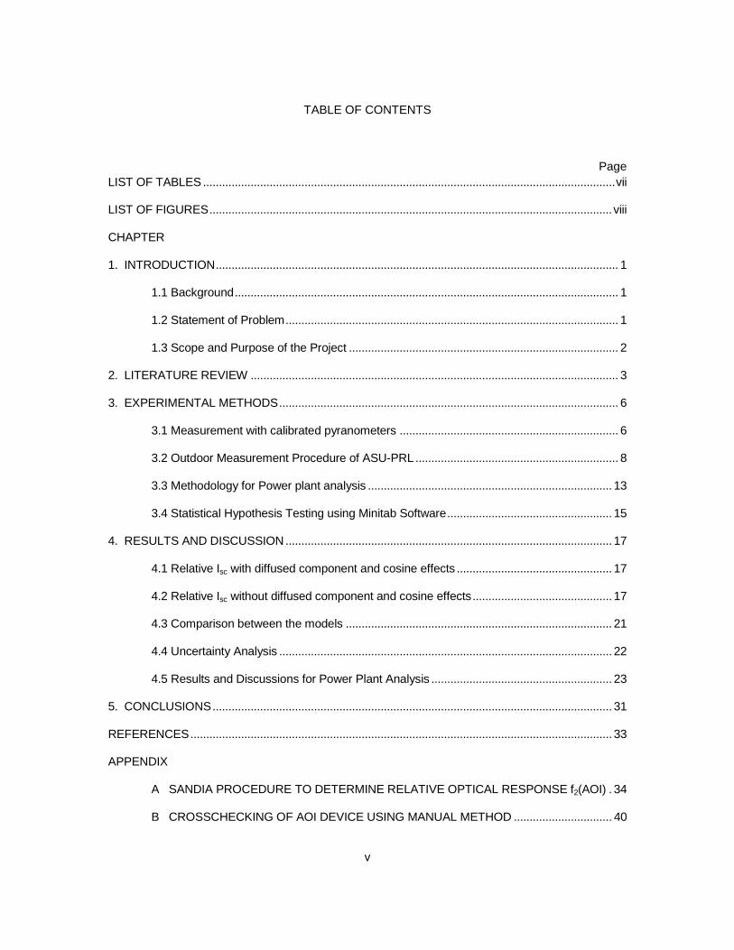
LIST OF TABLES

Table .......................................................................................................................................... Page

1. Model designation and module counts in power plant ............................................................... 14

2. Uncertainty of various uncertainty contributors in equations 4 and 5 ......................................... 22

3. Values for mean and median for each model ............................................................................. 25

4. Primary parameter and the primary visual defect causing the degradation in power for each

model ......................................................................................................................................... 29

E1.Comparison of Kipp & Zonen CMP21 verses Eppley PSP measured global irradiance in the

plane of array for 87% direct to global irradiance ratio .............................................................. 53

viii

LIST OF FIGURES

Figure ....................................................................................................................................... Page

1: (A) DC current transducers; (B) CR 1000 DAS with a multiplexer .............................. 10

2: (A) AOI device; (B) AOI device mounted on a plastic arm ........................................... 10

3: (A) Sundial ‘zeroed’ to AOI platform with no shadow present; B) AOI accuracy check on

mono-Si module using the sundial…………………………………………………………………..11

4: Angle of incidence measurement setup on a two-axis tracker .................................................. 11

5: Pictures of all models in APS-STAR power plant ...................................................................... 14

6: Relative Isc with diffused component and cosine effects ........................................................... 17

7: Relative Isc without diffused component and cosine effects – IEC method ............................... 19

8: Relative Isc without diffused component and cosine effects – Sandia method ........................ 19

9: Comparison between Eppley and Kipp & Zonen pyranometers – CdTe Module ...................... 20

10:Comparison between various models developed by different institutions ................................ 21

11:Uncertainties obtained as error bars presented for all modules ................................................ 23

12:Plot for I-V Parameters versus average annual degradation rates for all models ..................... 23

13:Histogram of degradation rates ................................................................................................. 24

14:Power Mean and Median for various models ............................................................................ 25

15:Plot for various I-V parameter degradation (%/year) for Model A13 ......................................... 26

16:Plot for various I-V parameter degradation (%/year) for Model B ............................................. 26

17:Plot for various I-V parameter degradation (%/year) for Model C12 ......................................... 27

18:Plot for various I-V parameter degradation (%/year) for Model D ............................................. 27

19:Plot for various I-V parameter degradation (%/year) for Model E ............................................. 28

20:Plot for various I-V parameter degradation (%/year) for Model F ............................................. 28

21:Plot for various I-V parameter degradation (%/year) for Model C4 ........................................... 29

A 1:Empirical f2(AOI) measurements by Sandia National Laboratories for conventional flat-plate

modules with a planar glass front surfaces. .............................................................................. 38

ix

Figure ......................................................................................................................................... Page

B 1:Comparison of relative optical responses obtained using the AOI hardware

and AOI calculation for a CdTe module with glass superstrate for

azimuth rotation(direct to global ratio was 0.89)…………………………...……………………..42

B 2:Comparison of relative optical responses obtained using the AOI hardware

and AOI calculation for a CdTe module with glass superstrate for

elevation rotation (direct to global ratio was 0.89) ................................................................... 42

C 1:Round 1 – Relative short circuit current verses AOI for five modules

(Multi-curve tracer method) ...................................................................................................... 46

C 2:Round 1 - Data for five modules where f2(AOI) was erroneously calculated

using Equation A6 (Multi-curve tracer method) ....................................................................... 47

D 1:Round 2 - Relative short circuit current verses AOI

for five modules (Data logger method) ..................................................................................... 49

D 2:Round 2 - Data for five modules where f2(AOI) was correctly calculated

using Equation A6 (Data logger method) ................................................................................ 50

E 1:Global irradiance as measured by the Kipp & Zonen CMP21 and

Eppley PSP pyranometer for 87% Edni/Epoa ......................................................................... 52

E 2:Comparison of Kipp & Zonen CMP21 verses Eppley PSP measured global irradiance

in the plane of array for 81% direct to global irradiance ratio .................................................. 54

E 3:Comparison of Kipp & Zonen CMP21 verses Eppley PSP measured global irradiance in

the plane of array for 2% direct to global irradiance ratio ........................................................ 55

F 1:Round 3 - Data for five modules where f2(AOI) was calculated when the tracker was

rotated in the opposite direction (East to West) ....................................................................... 57

F 2:Round 3 - Data for f2(AOI) calculated for CdTe from West to East compared to data

when the tracker was rotated in the opposite direction (East to West) .................................... 58

F 3:Round 3 - Data for f2(AOI) calculated for a-Si from West to East compared to data when the

tracker was rotated in the opposite direction (East to West) ................................................... 58

x

Figure ......................................................................................................................................... Page

F 4: Round 3 - Data for f2(AOI) calculated for CIGS from West to East compared

to data when the tracker was rotated in the opposite direction (East to West) ........................ 59

F 5: Round 3 - Data for f2(AOI) calculated for Mono-Si from West to East compared

to data when the tracker was rotated in the opposite direction (East to West) ........................ 59

F 6: Round 3 - Data for f2(AOI) calculated for Poly-Si from West to East compared

to data when the tracker was rotated in the opposite direction (East to West) ........................ 60

G 1: Degradation power versus degradation of I-V parameters for model A13 ............................. 62

G 2: Degradation power versus degradation of I-V parameters for Model B ................................. 62

G 3: Degradation power versus degradation of I-V parameters for model C12 ............................. 63

G 4: Degradation power versus degradation of I-V parameters for Model C4 ............................... 63

G 5: Degradation power versus degradation of I-V parameters for Model D ................................. 64

G 6: Degradation power versus degradation of I-V parameters for Model E ................................. 64

G 7: Degradation power versus degradation of I-V parameters for Model F ................................. 65

H 1: Pareto chart of defects for Model A13 .................................................................................... 67

H 2: Pareto chart of defects for Model B ........................................................................................ 67

H 3: Pareto chart of defects for Model C12 .................................................................................... 68

H 4: Pareto chart of defects for Model C4 ...................................................................................... 68

H 5: Pareto chart of defects for Model D ........................................................................................ 69

H 6: Pareto chart of defects for Model E ........................................................................................ 69

H 7: Pareto chart of defects for Model F ........................................................................................ 70

I 1: Plot for average annual degradation of I-V parameters for Model A13 .................................... 72

I 2: Plot for average annual degradation of I-V parameters for Model B ........................................ 72

I 3: Plot for average annual degradation of I-V parameters for Model C12 ................................... 73

I 4: Plot for average annual degradation of I-V parameters for Model C4 ..................................... 73

I 5: Plot for average annual degradation of I-V parameters for Model D ....................................... 74

I 6: Plot for average annual degradation of I-V parameters for Model E ........................................ 74

xi

Figure ......................................................................................................................................... Page

I 7: Plot for average annual degradation of I-V parameters for Model F ........................................ 75

J 1: Histogram of Power Degradation (%/Year) for Model A13 ...................................................... 77

J 3: Histogram of Power Degradation (%/Year) for Model B .......................................................... 77

J 4: Histogram of Power Degradation (%/Year) for Model C12 ..................................................... 78

J 5: Histogram of Power Degradation (%/Year) for Model C4 ....................................................... 78

J 6: Histogram of Power Degradation (%/Year) for Model D ......................................................... 79

J 7: Histogram of Power Degradation (%/Year) for Model E .......................................................... 79

J 8: Histogram of Power Degradation (%/Year) for Model F .......................................................... 80

K 1: Degradation values of Isc, Voc and Fill Factor per year pasted on Minitab ............................. 82

K 3: Options button for performing 2 Sample t test in Minitab ........................................................ 82

K 4: Samples placed on two different columns in the dialog box are compared ............................ 83

K 5: A symbol chosen for implementing the alternative hypothesis ............................................... 83

K 6: Window containing the P-Value .............................................................................................. 84

1

Chapter 1

1. INTRODUCTION

1.1 Background

The angle of Incidence (AOI) of a PV module can be defined as the angle between the

incident beam of light and a line perpendicular to the plane of the module. Light entering the

module has to pass through a glass cover, encapsulant layer, and an antireflective coating layer

before reaching the energy producing material of the solar cell. Photovoltaic module ratings

provided by the manufacturers are performed at STC conditions, with irradiance being 1000

W/m2, 25

oC cell temperature. These ratings are measured at an incident angle of 0⁰, whereas in

an actual field, the angle of incidence varies resulting in higher losses than the rated values. This

simply implies that for AOI values greater than zero, the module’s performance will be lower than

the one rated at STC conditions. The electrical characteristics of PV modules are affected during

such real-time conditions, especially the current (amperes). The first part of this work

investigates the influence of AOI on PV modules’ performance.

In PV power plants, the average annual power degradation rate is used as one of the

primary metrics to determine and predict the total energy produced by the system. The

degradation rate is dictated by the module design quality, manufacturing quality, and site-specific

environmental conditions. The power degradation could be attributed to one or more of the

performance parameters: current, voltage or fill factor. The second part of this thesis investigates

the distribution of these performance parameters which influence the power degradation of PV

modules.

1.2 Statement of Problem

The main objective of the first part is to test and validate the IEC 61853-2 (draft) standard

procedure for measuring the effect of AOI on PV modules. The following statement from IEC

61853-, 2 “ for the flat glass superstrate modules, the AOI test does not need to be performed;

2

rather, the data of a flat glass air interface can be used”, needs to be validated by comparing the

plots obtained from the IEC 61853-2 model complying with those plots obtained using theoretical

and empirical models. The relative light transmission plots for all modules with glass superstrates

should be identical.

The main purpose of the second part of the thesis is to:

To check whether the modules degraded at a constant rate or at a highly varied rate by

the means of statistical analysis.

Statistically analyze the possible visual factors that cause power degradation.

1.3 Scope and Purpose of the Project

Due to the short project period available to execute this labor intensive project, this

project was carried out jointly in collaboration with another MS thesis student, Brett Knisely. The

scope of the first part of this thesis and Mr. Knisely’s thesis is to test and validate AOI test

methods and models identified in draft standard IEC 61853-2. Mr.Knisely’s thesis is expected to

be submitted in summer 2013 and will uniquely focus on the quantum efficiency of PV module

cells. The second part of this thesis will uniquely focus on analyzing a power plant and

determining the major factors causing degradation in power. The current-voltage (I-V) data

obtained by previous researchers of ASU-PRL was analyzed and distributions of power

degradation in power per year were plotted for each model. Additionally, degradations in the ISC,

VOC and fill factor (FF) per year were obtained using statistical hypothesis testing.

3

Chapter 2

2. LITERATURE REVIEW

The PV industry currently aims to evaluate modules beyond STC conditions by studying

the factors affecting module performance and designing a proper test method for measuring the

effects of angles of incidence (AOI). The power generated by the module is directly related to the

irradiance incident upon it. Thus, prior research conducted by Sandia National Laboratories

determined that two factors which complicate the characterization of modules are: 1) variations in

solar spectrum and 2) optical properties with the AOI. Higher angle of incidence considerably

lowers the module’s power. The performance of a PV module is reported at 1.5 air mass, with air

mass characterizing the solar spectrum after sunlight has travelled through the atmosphere. The

air mass quantifies the reduction in the amount of light as it passes through the atmosphere and

is absorbed by air and dust. When the sun is directly overhead, air mass is a unity. The

magnitude of change in the sunlight’s spectrum also has a major impact on performance. A

procedure for measuring the effect of AOI on the modules was developed using empirical

equations. In other studies, researchers had developed an analytical model for finding the annual

angular losses due to real-world conditions. This model is a function of tilt, location, and season,

and concurs with the model developed by previous researchers. The amount of sunlight reaching

the solar cells is dependent upon the reflected and transmitted fractions of incident light. The

following two module design elements influence module performance, 1) transmittance ( light

passing through the superstrate, and encapsulant), and 2) reflectance(scattered light bouncing

through and around the: superstrate and encapsulant, the air/superstrate, and encapsulant/cell

interfaces. These are a function of AOI. The effect of AOI is heavily dependent upon the surface

roughness and the antireflective coatings of the superstrate.

The short circuit current of a PV module is affected by: the mechanical/geometrical effect

and the optical effect. The geometrical effect is best described as the orientation of the module

with respect to incident light. The geometrical effect is also known as the cosine effect and states

4

that the irradiance falling on the module decreases as the AOI increases. The irradiance is

directly related to cosine (AOI). The second factor influencing AOI is the optical effects, which

describes the surface characteristics of the module. The majority of PV manufacturers constantly

research to improve the surface characteristics of modules by modifying the anti-reflective

coatings, and/or glass type (rolled or textured glass).

The effects of AOI on short circuit current were tested for five different module

technologies: amorphous silicon (a-Si), cadmium telluride (CdTe), copper indium gallium selenide

(CIGS), mono crystalline silicon (Mono-Si) and polycrystalline silicon (Poly-Si).

To make a module durable for field use, failure rates needs to be kept low. Reliability

studies play a significant role in analyzing and modifying the product for better success in the

commercial market. The performance of a module at its rated power for the claimed number of

years is the key for reliability studies. After extensive research in reliability, failures during the

initial stages of the module’s life have been reduced. The failure rate increases rapidly during the

final stages of a module’s life. Plotting the failure rate with respect to product life would give us a

bath tub curve. Module lifetime field testing requires a long time, which is not possible in today’s

highly competitive world. Increasing stress levels beyond the design limits accelerate failures in

the product. This is known as accelerated testing and is employed extensively in the industry.

These tests help in identifying and correcting defects which would reduce module mortality rates.

Several research studies have analyzed the factors affecting module degradation using historical

field data. One such research involved the analysis of 9.2 KWp PV array situated near Trinidad,

CA, on the Pacific coast. The average power degradation rate for these modules was found to be

decreased by 4.39% after 11 years in the field. The major cause for degradation was due to

short circuit current which decreased by 6.38% after 11 years. On analyzing the same array after

20 years in the field, the power drop was found to be 16.13 %. Again, the major factor was found

to be current drop due to browning or discoloration of the encapsulant.

5

The National Renewable Energy Laboratory (NREL) researched 12 different

monocrystalline and polycrystalline modules and found that the modules degraded less than 0.5

% per year with the main cause of power degradation being a drop in short circuit current.

Another research project performed by NREL on 2000 modules of various technologies found

that the degradation rate was less than 1 % per year. The crystalline modules degraded largely

due to a drop in the ISC values, and to some extent, the fill factor. The thin film module

technologies degraded due to a decline in the fill factor, especially in humid climates. The current

research was performed on 1700 crystalline silicon modules which were in hot and dry climatic

field conditions for over 13 years.

6

Chapter 3

3. EXPERIMENTAL METHODS

3.1 Measurement with calibrated pyranometers

During the course of this project, the testing and analysis procedure was performed in

three rounds, with the third round resulting in accurate and satisfying data. The data obtained in

the third round of testing and analysis is presented in this chapter. The data obtained in the

previous two rounds is provided for reference in Appendices C and D of this thesis.

Test Apparatus:

The following are the types of test apparatus used in the experiment along with a brief

description.

1) Irradiance Sensors: The global and direct irradiances can be measured using these

devices. According to the measurement procedure of standard IEC 61853-2 (draft), a

combination of pyranometer (for measuring global irradiance) and pyrheliometer (for

measuring direct normal irradiance) were used.

2) Thermal Sensors: The ambient, module, and reference cell temperature are measured

using T-type thermocouples.

3) Data acquisition system: A data acquisition system was used to collect and store data

from the modules using irradiance and thermal sensors.

4) Two-axis Tracker: All the test modules were placed on a two axis tracker, so that the

azimuth and tilt could be controlled.

5) AOI measuring device: This device is used to determine the tilt angle as well as to verify

the co planarity of test modules and irradiance sensors.

Test Setup:

1) The front surface of the test modules should be thoroughly cleaned.

2) The test modules should be mounted on a two-axis tracker securely.

7

3) The test modules and all the sensors should be connected to the data acquisition

system.

Measurement Procedure:

1) If the diffused component does not exceed 10% of the total irradiance, the short circuit

current measured (Isc(θ )) can be used to calculate the relative angular light transmission

data, τ(θ). But, if the diffused component exceeds 10% of the total irradiance, then the

short circuit current (Isc (θ)) should be corrected for the calculation of τ (θ). This

correction is dependent on the type of sensor used.

2) If the irradiance sensor is a reference cell: The diffused component should not be more

than 10% of the total irradiance obtained during the measurement of Isc (θ). If the

diffused component exceeds 10%, it can subtracted from global irradiance after

measuring the angular response with blocked direct light component or by blocking the

diffused component by reducing the field of view of the diffused component.

3) If the irradiance sensors are pyranometers and pyrheliometers: The diffused light striking

the module would be given as :

Gdiff=Gtpoa-Gdni cos (θ) (1)

Where:

“Gtpoa” is the total irradiance in the plane of the module, as measured by a pyranometer

“Gdni” is the direct light component measured by the pyrheliometer.

“Θ” is the tilt angle between the direct irradiance falling on the module and the normal of

module.

The short circuit current obtained from direct light component can be obtained from the

diffused light component which is given as follows:

Isc (θ) = Isc measured (θ) (1- Gdiff / Gtpoa) (2)

The relative angular light transmission (or relative angular optical

response) into the module is given by:

τ (θ) = Isc(θ)/(cos (θ) Isc(0)) (3)

8

3.2 Outdoor Measurement Procedure of ASU-PRL

This experiment was performed at ASU-PRL, and the measurements obtained in

accordance with standard IEC 61853-2 (draft). The details of the apparatus used in the

experiment are given as follows:

1) Test Modules: Five different technologies were used: monocrystalline silicon (Mono-Si),

polycrystalline silicon (Poly-Si), amorphous silicon (a-Si), cadmium telluride (CdTe) and

copper indium gallium Selenide (CIGS). Glass was the superstrate in all the cases.

2) Irradiance Sensors: A reference cell (Poly-Si), two pyranometers from 2 manufacturers

namely Eppley PSP and Kipp & Zonen and pyrheliometer from Kipp & Zonen were used.

The data obtained using the pyranometers and pyrheliometers were later processed.

3) Thermal Sensors: T-Type thermocouples manufactured by Omega were placed at the

centre of the back sheet of the modules with the help of a thermal tape. The accuracy

was given to be +/- 1° C above 0°C.

4) Data acquisition system: CR1000 manufactured by Campbell Scientific was used to

collect data. A magnetic DC current transducer (Figure 1A) was used to measure the

short circuit current. This equipment is kept in an air conditioned room for maintaining a

constant operating temperature. The accuracy of this equipment is 1%. A linear relation

was given for the current passing through the transducer and its output voltage. All the

data was recorded and stored in the data acquisition system.

5) Two axis tracker: All the modules, irradiance sensors and the AOI measuring devices

were mounted on the two axis tracker. Usually a tracker has full range of motion in order

to achieve high angles of incidence during any time of the day. The tracker was limited to

65° of rotation about elevation angle and 180° about the Azimuth angle. Higher AOI was

obtained by starting the experiment at approximately 2:30pm (for our setup) so that the

full range in azimuth could be utilized. Since the direct irradiance was necessary to be

obtained, a pyrheliometer was allowed to track the sun.

9

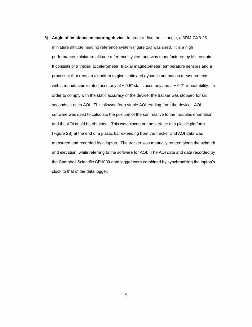
6) Angle of Incidence measuring device: In order to find the tilt angle, a 3DM-GX3-25

miniature altitude heading reference system (figure 2A) was used. It is a high

performance, miniature altitude reference system and was manufactured by Microstrain.

It consists of a triaxial accelerometer, triaxial magnetometer, temperature sensors and a

processor that runs an algorithm to give static and dynamic orientation measurements

with a manufacturer rated accuracy of ± 0.5° static accuracy and a ± 0.2 repeatability. In

order to comply with the static accuracy of the device, the tracker was stopped for six

seconds at each AOI. This allowed for a stable AOI reading from the device. AOI

software was used to calculate the position of the sun relative to the modules orientation

and the AOI could be obtained. This was placed on the surface of a plastic platform

(Figure 2B) at the end of a plastic bar extending from the tracker and AOI data was

measured and recorded by a laptop. The tracker was manually rotated along the azimuth

and elevation, while referring to the software for AOI. The AOI data and data recorded by

the Campbell Scientific CR1000 data logger were combined by synchronizing the laptop’s

clock to that of the data logger.

10

(A) (B)

Figure 1: (A) DC current transducers; (B) CR 1000 DAS with a multiplexer

(A) (B)

Figure 2: (A) AOI device; (B) AOI device mounted on a plastic arm

To ensure that all reference devices and modules are coplanar with respect to each

other, the altitude heading device was placed on each module and the AOI could be obtained and

checked for consistency. The presence of any magnetic material near the device would

marginally affect the accuracy. To check the co-planarity, the tracker was set to automatic mode

and was allowed to track at an angle normal to the incident light.

11

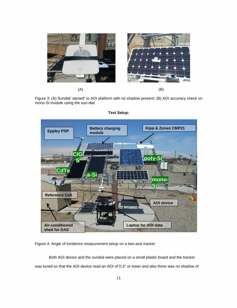
(A) (B)

Figure 3: (A) Sundial ‘zeroed’ to AOI platform with no shadow present; (B) AOI accuracy check on mono-Si module using the sun-dial

Test Setup:

Figure 4: Angle of incidence measurement setup on a two-axis tracker

Both AOI device and the sundial were placed on a small plastic board and the tracker

was tuned so that the AOI device read an AOI of 0.3° or lower and also there was no shadow of

a-Si

Battery charging module

Air-conditioned shed for DAS

Laptop for AOI data

Reference Cell

CIGS

CdTe

mono-Si

poly-Si

Kipp & Zonen CMP21 Eppley PSP

AOI device

12

the sundial (Figure 3A).Then the sundial was placed on each module at various positions such as

center and corner. The shadow was obtained for each position and as shown in the equation

below, the point of the tracker with the longest shadow length represented least accurate point

with respect to AOI (AOImax error). The maximum shadow length was found to be 0.7°. Given that

the initial AOI reading was a maximum of 0.3°, the projected maximum uncertainty for was +/-

1.0°.

Measurement Procedure

Data was collected as quickly as possible to mitigate the effects due to module

temperature and solar spectral variations. The following factors were given primary importance

during the experiment.

1) Soiling: Dust can be a major influence on the irradiance reaching the module’s surface.

The modules were cleaned before data collection.

2) Reflection from surroundings: Items or objects of high reflectance should not be

present when the data is being collected. No significant reflections were observed in the

surroundings. Protruding devices were removed from the tracker and the ground was a

flat gravel surface.

3) Standard and constant irradiance: The experiment was performed during clear sky

conditions when the ratio of direct normal irradiance to the global normal irradiance was

greater than 0.85. This ratio is a major factor during the measurement, especially at

higher AOI.

4) Standard and constant spectrum: Ideally, the experiment must be performed during

solar noon to reduce the effect of spectral variation during the test period. Since there

was limitation with the tracker movements, the test was performed around 2:30 pm to

utilize the full range of the tracker. However, the test was completed in 10 minutes so

that a constant spectrum could be maintained throughout the experiment. The AOI was

varied by moving the tracker in azimuth and elevation from west to east to angles close to

90°.

13

5) Standard and constant temperature: The measurements should be done at a constant

module temperature. But, when the AOI varies, the modules’ temperature varies

because of changes in the irradiance. A thermocouple was placed on the back sheet of

the modules and the temperature was recorded throughout the experiment. From the

temperature coefficient obtained while taking baselines for each module, the short circuit

current was corrected for 25°C to remove the influence of varying temperature during the

experiment.

6) Maximum number of data points: The larger the data collected, higher the accuracy of

the measurements. The data logger collected data at a frequency of 30 seconds, and a

large amount of data was collected to increase the accuracy of measurements. To obtain

data with nearly constant irradiance and air mass conditions, the tracker was moved 5°

every 30 seconds up to AOI close to 85° (or as far as the tracker would allow). Hence

the Isc vs. AOI graph was plotted with a minimum of 18 data points.

3.3 Methodology for Power plant analysis

The I-V data collected for 1900 modules at the power plant was translated to STC

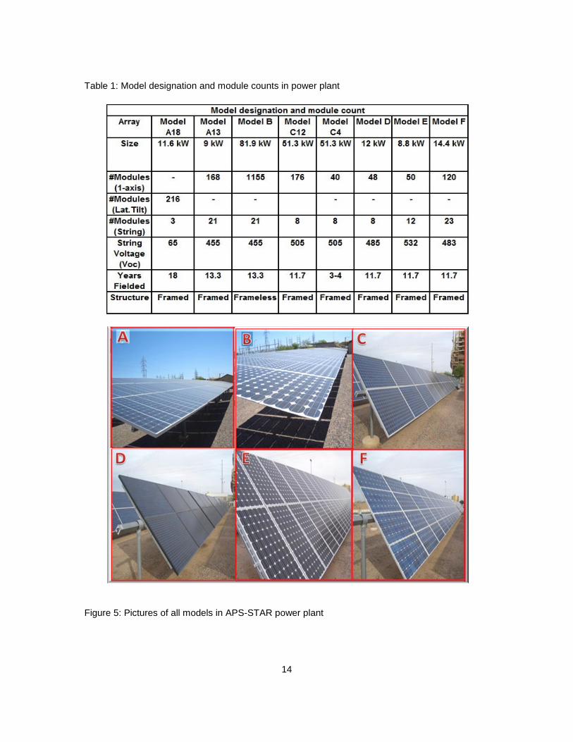
conditions by a procedure developed at the Arizona State University. Table 1 shows the module

models and the physical characteristics of the power plant array. In order to not disclose the

names of the module manufacturers, the modules were given model names from A to F. Model A

and F are further segregated based on the number of years in the field. The figure 5, shows the

different models analyzed at the power plant.

14

Table 1: Model designation and module counts in power plant

Figure 5: Pictures of all models in APS-STAR power plant

15

All these modules, shown in Table 1 (except A18 modules) are to be statistically

analyzed to identify the performance parameter causing power degradation. This part of the

project required the process of statistical hypothesis testing using Minitab software.

3.4 Statistical Hypothesis Testing using Minitab Software

The use of statistics to determine the chances for a given condition to be rejected or not

rejected is called hypothesis testing. The following are the steps involved in hypothesis testing

using Minitab software.

1) Firstly, the null hypothesis and alternative hypothesis need to be clearly defined. Null

hypothesis can be defined as a general condition and is denoted as H0. When the

hypothesis does not satisfy the null hypothesis, it is called as Alternative hypothesis and

is denoted as H1. The alternative hypothesis becomes true only when the probability

does not exceed the identified significance level (in this case α=0.05). The null

hypothesis can be mathematically defined as, H0: µ0=µ1, where: µ0, µ1 are mean of

population 1 and 2 respectively. Whereas, the mathematical definition for alternative

hypothesis can be written as H1: µ0>µ1 or µ0<µ1 or µ0≠µ1.

2) The degradation per year values for short-circuit current, open circuit voltage and fill

factor are copied into the Minitab worksheet. A two sample t test is performed upon the

selected columns. Columns like degradation for Isc with degradation for fill factor and

degradation for Isc with degradation for Voc are compared. The options button in the 2

sample t test dialog box consists of various comparison symbols and usually < or >

symbols are chosen for comparison.

3) Once the test has been performed, a working window pops up with various numeric

values such as test statistic value and the probability value. The probability value

obtained should be compared with the significance level (i.e. α=0.05). If the P value is

smaller than that of significance value, the alternative hypothesis becomes true and the

null hypothesis can be rejected. By this statistical approach the parameter affecting the

16

power drop could be found. An example of hypothesis testing has been demonstrated in

appendix K.

A graphical method to find the factor affecting power drop is achieved by plotting graphs

with power drop (on the X-axis) and other parameters like short circuit current, open circuit

voltage and fill factor ( on the Y-axis). The graph showing a linear increase will be the factor

affecting the power drop. Statistical approach is a scientific and reliable approach to identify the

parameters(s) influencing power loss. The plots for graphical methods for all the models are

provided in the appendix section I.

17

Chapter 4

4. RESULTS AND DISCUSSION

4.1 Relative Isc with diffused component and cosine effects

When the ratio of direct normal irradiance (Gdni) to global irradiance was 87%, the first set

of data was collected. For each angle of incidence, the Isc data was measured and collected.

Figure 5 shows the relative Isc which contains both the diffused components and the cosine

effects. The plot obtained shows that the data is identical for all the 5 type of technologies. The

true Isc value obtained (relative optical response) is free from diffused component and the cosine

effect. Hence the Isc data shown in the Figure 6 has to be corrected.

Figure 6: Relative Isc with diffused component and cosine effects

4.2 Relative Isc without diffused component and cosine effects

According to the requirements of the standard, the diffused component of incident light

should not be greater than 10% of the total irradiance during the experiment. In order to remove

the influence of diffused component, the data should be corrected. This can be done either by

0

0.2

0.4

0.6

0.8

1

1.2

0 20 40 60 80 100

Rela

tive I

sc

AOI (degrees)

CdTe

A-Si

CIGS

Mono-Si

Poly-Si

18

using the reference cell method or the pyranometer/pyrheliometer method as prescribed by the

standard. In the reference cell method, the procedure describes: “If the diffused component

exceeds 10%, it can be subtracted after measuring the angular response with blocked direct light

component or the diffuse component can be blocked to below 10% by reducing the field of view

of the diffuse component, for example by collimating the incident light reaching the test module.”

The Isc obtained from this method does not contain any diffused component as it is subtracted

from the global irradiance.. The Isc (θ) can be directly used in equation 3 to obtain the relative

optical response which does not include the diffused component and the cosine effects.

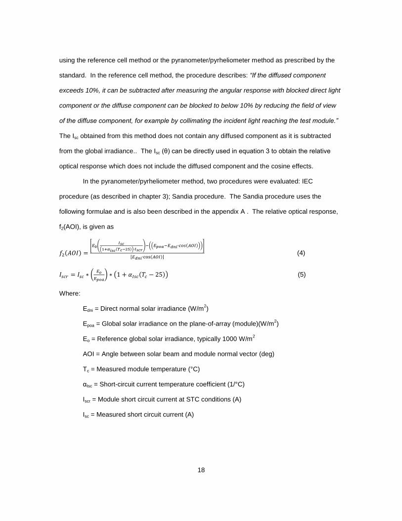
In the pyranometer/pyrheliometer method, two procedures were evaluated: IEC

procedure (as described in chapter 3); Sandia procedure. The Sandia procedure uses the

following formulae and is also been described in the appendix A . The relative optical response,

f2(AOI), is given as

(4)

(5)

Where:

Edni = Direct normal solar irradiance (W/m2)

Epoa = Global solar irradiance on the plane-of-array (module)(W/m2)

Eo = Reference global solar irradiance, typically 1000 W/m2

AOI = Angle between solar beam and module normal vector (deg)

Tc = Measured module temperature (°C)

αIsc = Short-circuit current temperature coefficient (1/°C)

Iscr = Module short circuit current at STC conditions (A)

Isc = Measured short circuit current (A)

19

Figure 7: Relative Isc without diffused component and cosine effects – IEC method

Figure 8: Relative Isc without diffused component and cosine effects – Sandia method

0

0.2

0.4

0.6

0.8

1

1.2

0 20 40 60 80 100

Rela

tive R

esp

on

se

AOI (degrees)

CdTe

A-Si

CIGS

Mono-Si

Poly-Si

0

0.2

0.4

0.6

0.8

1

1.2

0 20 40 60 80 100

Rela

tive O

pti

cal

Resp

on

se

f2(A

OI)

AOI (degrees)

CdTe

A-Si

CIGS

Mono-Si

Poly-Si

20

The plots obtained from IEC procedure (equations 1, 2 & 3) and Sandia procedure (equation 4 &

5) are shown in Figures 7 & 8, respectively. Both these procedure have similar results. Figure 9

shows the data can be influenced at higher values of AOI (>60 o) by the type of pyranometer due

to the sensitivity of AOI on the calibration factors of the pyranometers above 60o.

Figure 9: Comparison between Eppley and Kipp & Zonen pyranometers – CdTe Module

In both the reference cell and pyranometer/pyrheliometer method, there are pros and

cons. With the reference cell method, there is no spectral mismatch error (if the test is long)

between the reference cell and the test module when a matching reference cell technology is

used. However it requires additional module measurements with collimated lights or blocked

lights. In the pyranometer/pyrheliometer method, extra module measurements are not required.

But, there is spectral mismatch error between the test modules, pyranometer and pyrheliometer,

if the air mass exceeds 1.5. This error can be considered of second order issue with no impact

on the final data if the experiment is of short duration.

0.0

0.2

0.4

0.6

0.8

1.0

1.2

0 20 40 60 80 100

Rela

tive L

igh

t Tra

nsm

issio

n

AOI (degrees)

IEC Model (Eppley pyranometer)

IEC Model (Kipp & Zonen pyranometer)

21

4.3 Comparison between the models

The data obtained from f2 (AOI) for the modules with glass superstrate, Sandia National

Laboratories found a generic polynomial model as shown in equation 6 (see Appendix A for

details)

f2(AOI) = 1-2.4377E-3(AOI) +3.1032E-4(AOI)2-1.2458E-5(AOI)

3+2.1122E-7(AOI)

4-1.3593E-

9(AOI)5 (6)

Many theoretical AOI models have been developed for the air-glass interface. The data

obtained from Sandia model and the IEC model for a glass superstrate (say CdTe) is compared

with the generic polynomial model of Sandia and Martin and Ruiz AOI model for air-glass

interface. All the plots are found to be identical with each other confirming that the relative optical

response is dictated by the air-glass interface. The draft standard states: “For modules with a flat

uncoated front glass plate made of standard solar glass, the relative light transmission into the

module is primarily influenced by the first glass-air interface. In this case, the test does not need

to be performed; rather, the data of a flat glass air interface can be used.” The experimental data

and the theoretical model confirm and validate the above statement.

Figure 10: Comparison between various models developed by different institutions

0.0

0.2

0.4

0.6

0.8

1.0

1.2

0 20 40 60 80 100

Re

lati

ve

Op

tic

al

Re

sp

on

se

f2(A

OI)

AOI (degrees)

IEC Model

Sandia model

Sandia Generic Model

22

To obtain accurate results, as in the case of non-glass (including AR coated glass) or

non-planar (non-flat) glass superstrate modules, the approach suggested by Sandia National

Laboratories may be followed (see appendix A). The results are similar for flat air-glass interface

modules, the reference module (flat glass with matched cell technology) and the module under

test can be analyzed and experimented simultaneously to remove any data processing errors.

4.4 Uncertainty Analysis

Precautions were taken to increase the accuracy of the procedure and test setup. For

equations 4 and 5, each uncertainty contributor was taken into account and the magnitude of

associated uncertainty was assigned based on the calibration report specifications. The table for

uncertainties is given below in Table 2.

Table 2: Uncertainty of various uncertainty contributors in equations 4 and 5

Uncertainty Contributor (Ui) Uncertainty

Isc (Uisc) 1.000%

Global Irradiance (Uepoa) 1.400%

Temperature Coefficient (Ualpha) 0.010%

Module Temperature (Ut) 0.75%

Direct Irradiance (Udni) 1.100%

Angle of Incidence (UAOI) 1.0%

The uncertainty for f2 (AOI) was taken as the square root of the sum of squares of the

estimates of uncertainty times the squares of the corresponding coefficients of sensitivity. By

taking the derivative of f2 (AOI) equation with respect to the uncertainty contributor, the sensitivity

coefficients can be found.

(7)

23

Figure 11: Uncertainties obtained as error bars presented for all modules

4.5 Results and Discussions for Power Plant Analysis

Figure 12: Plot for I-V Parameters versus average annual degradation rates for all models

0

0.2

0.4

0.6

0.8

1

1.2

0 20 40 60 80 100

Rela

tive O

pti

cal

Resp

on

se

f2(A

OI)

AOI (degrees)

CdTe

A-Si

CIGS

Mono-Si

-2

-1

0

1

2

3

4

5

0 2 4 6 8

Avera

ge D

eg

rad

ati

on

R

ate

(%

/ye

ar)

Parameter

Degradation Rate (%/year) vs. Various I-V Parameters

A-13

B

C-12

C-4

D

E

F Pmax Isc Voc FF Imp Vmp

24

The uncertainties obtained are presented as error bars in Figure 10 for all types of

module technologies. The uncertainty of f2(AOI) increases with increasing AOI. For this

experiment, a single sensitivity factor for the pyranometers for all values of AOI was used. But

still the sensitivity increases slightly with AOI going beyond 60 o. Therefore the uncertainty

increases with increasing AOI. From the data collected by the previous researcher, the above plot

has been constructed. The annual mean and median degradation rates for each model are

included in the appendix.

Figure 13: Histogram of degradation rates

The histogram for all the modules analyzed is given below with a distribution fit. The

histogram in figure 13 shows a mean and median degradation rates for 1757 modules, except the

A18 fixed tilt modules, which were not considered for the entire analysis. It shows a median

degradation rate of 1.48% per year. The histogram also indicates the modules are degrading

with a mean of 1.54% per year.

25

Table 3: Values for mean and median for each model

Model Degradation of Power (%/Year)

Mean Median

A13 2.27 2.20

B 1.53 1.51

C12 0.77 0.59

C4 4.25 4.76

D 0.84 0.50

E 0.52 0.55

F 1.40 1.29

Figure 14: Power Mean and Median for various models

The mean and median of these modules should be compared to determine the

degradation rate per year of all modules in a particular model is at a same rate. The histogram

for degradation of power for each model is shown in appendix J. The table 3 shows the mean

and median values for all the models. The mean and median data are closely matching and it

0

1

2

3

4

5

6

7

8

De

gra

da

tio

n o

f P

ow

er

(%

/Ye

ar)

Parameters

Power Mean and Median for Various Models

Mean

Median

A13 B C12 C4 D E F

26

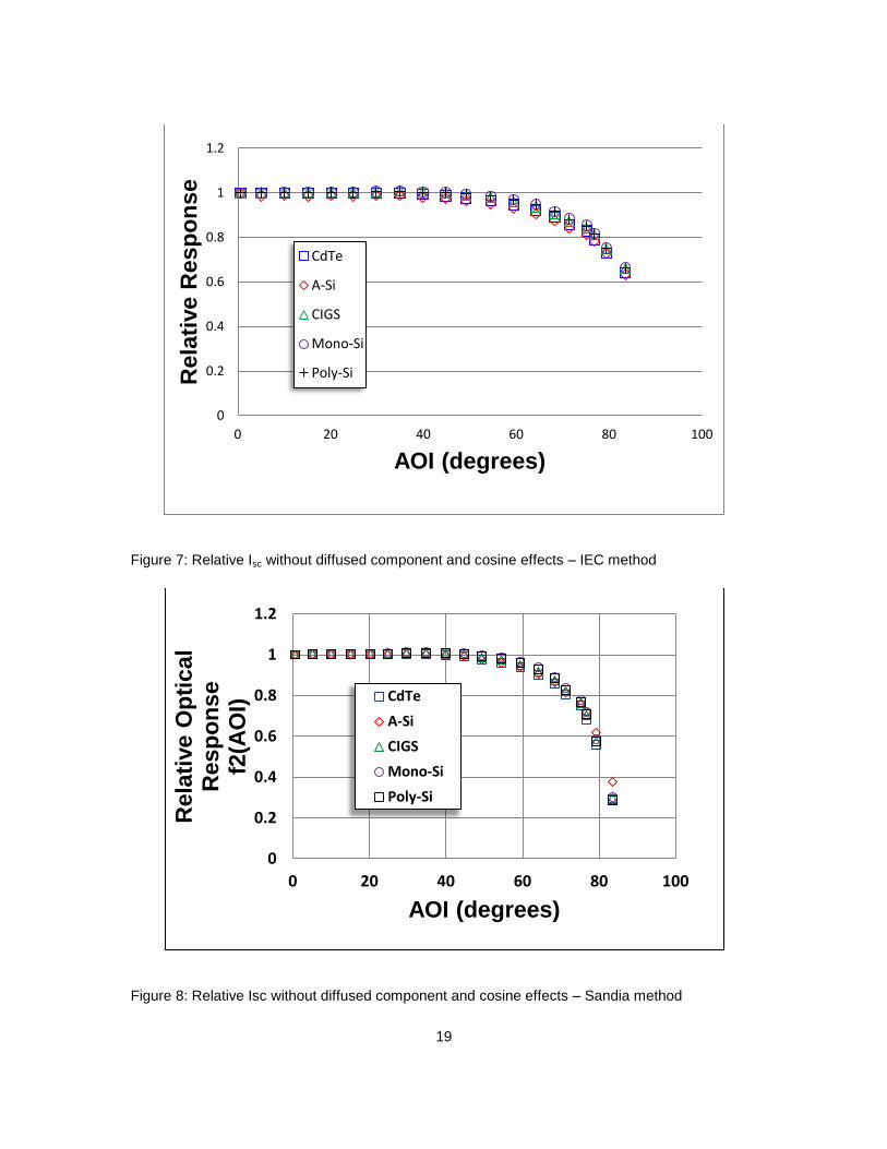
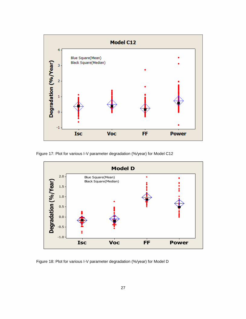
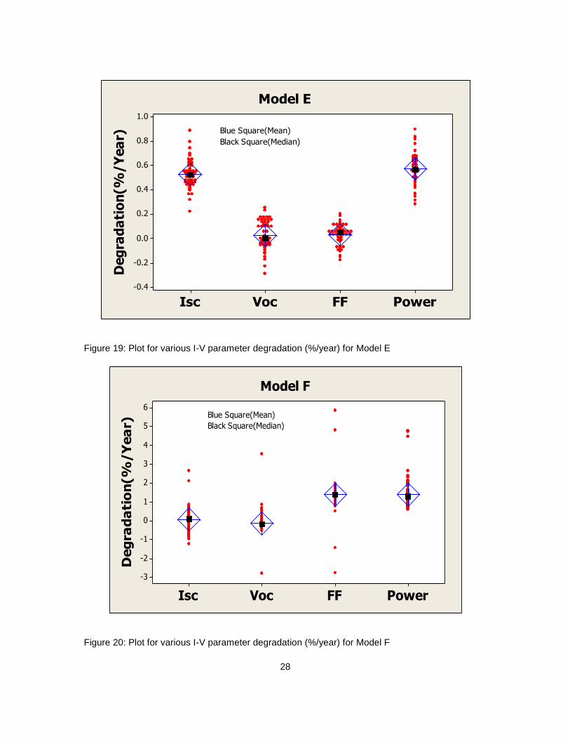
indicates that the data is not significantly skewed. The plots for mean and median for all models

are shown below in Figure 15 through Figure 21.

Figure 15: Plot for various I-V parameter degradation (%/year) for Model A13

Figure 16: Plot for various I-V parameter degradation (%/year) for Model B

PowerFFVocIsc

6

5

4

3

2

1

0

-1

-2

Deg

rad

ati

on

(%

/Y

ea

r) Black Square(Median)

Blue Square(Mean)

Model A13

PowerFFVocIsc

3

2

1

0

-1

-2

Deg

rad

ati

on

(%

/Y

ea

r)

Model B

Black Square(Median)

Blue Square(Mean)

27

Figure 17: Plot for various I-V parameter degradation (%/year) for Model C12

Figure 18: Plot for various I-V parameter degradation (%/year) for Model D

PowerFFVocIsc

2.0

1.5

1.0

0.5

0.0

-0.5

-1.0

Deg

rad

ati

on

(%

/Yea

r)

Model D

Black Square(Median)

Blue Square(Mean)

28

Figure 19: Plot for various I-V parameter degradation (%/year) for Model E

Figure 20: Plot for various I-V parameter degradation (%/year) for Model F

PowerFFVocIsc

1.0

0.8

0.6

0.4

0.2

0.0

-0.2

-0.4

Deg

rad

ati

on

(%/Y

ea

r)

Model E

Black Square(Median)

Blue Square(Mean)

PowerFFVocIsc

6

5

4

3

2

1

0

-1

-2

-3

Deg

rad

ati

on

(%

/Y

ea

r)

Model F

Black Square(Median)

Blue Square(Mean)

29

Figure 21: Plot for various I-V parameter degradation (%/year) for Model C4

Table 4: Primary parameter and the primary visual defect causing the degradation in power for each model

Model [Years]

Average Pmax

Degradation(%/Year)

Order of Statistical

Parameters Affected

Order of Statistical

Visual Defects

Potential Primary

Reasons for Pmax

Degradation

A13 [13] (glass/polymer)

2.29 FF>> Isc > Voc DE, SD

Series resistance

increase(SBD) DE

B [12] (glass/polymer)

1.53 FF >> Isc > Voc DE, MSW

Series resistance increase

(SBD), DE

C12 [12] (glass/glass)

0.77 Voc > Isc = FF DLM, BC,

HS DLM

C4 [4] (glass/glass)

4.14 FF > Voc >> Isc BC, DLM,

HS Unknown

D [12] (glass/polymer)

0.83 FF >> Isc = Voc DE Series

resistance increase(SBD)

E [12] (glass/polymer)

0.57 Isc >> FF = Voc MSW MSW

F [12] (glass/polymer)

1.40 FF >> Isc = Voc MD, SD

Series resistance increase (SBD)

PowerFFVocIsc

10.0

7.5

5.0

2.5

0.0

-2.5

-5.0

Deg

rad

ati

on

(%

/Y

ea

r)

Model C-4

Dotted Line(Median)

Undotted Line(Mean)

30

From the table and graphs above we clearly see that all mean and median are nearly

equal for all modules of a particular model.

The table below shows the primary factor and major visual defect that is causing the drop

in power for modules of each model. The abbreviations of the defects found statistically are as

follows: Discoloration of Encapsulant (DE), Seal Deterioration (SD), Minor Substrate Warping

(MSW), Delamination (DLM), Broken Cells (BC), Hotspots (HS), Metallization Discoloration (MD),

and Solder Bond Deterioration (SBD).

The primary visual defects are shown on a Pareto charts for each model in Appendix H.

31

Chapter 5

5. CONCLUSIONS

Validation of standard IEC 61853-2 (draft) for measuring the effect of AOI on PV modules

was accomplished using outdoor test method for five different technologies. The important

results obtained are:

With glass as superstrate for all five different technologies tested, the relative light

transmission plots are practically the same. The air-glass interface of the PV modules

primarily governs reflective losses as demonstrated with the theoretical curves obtained

at the air-glass interface.

Models developed by Sandia National Laboratories and the theoretical air-glass interface

models for glass superstrate matched with the relative transmission plots that was

obtained using the IEC 61853-2 model.

The analysis and conclusion of this study confirms and validates the statement “for the

flat glass superstrate modules, the AOI test does not need to be performed; rather, the

data of a flat glass air interface can be used.” delineated in the IEC 61853-2 standard is

accurate.

In order to test a non-glass or non-planar module and get an accurate result, the

reference module (flat glass superstrates and matched cell technology) approach can be

done in accordance with the procedure described by Sandia National Laboratories.

The important conclusions obtained from the power plant study were:

Significant number of modules falls close to the mean value (as indicated by the median

value) of degradation rate but a few modules have high degradation rates. This indicates

that the string power could be lower from that of the sum of individual power of the

modules in that string.

32

The primary causes for power degradation in all glass/polymer modules appear to be due

to the fill factor loss and short circuit current loss. The primary degradation modes

attributed to these losses are solder bond deterioration and encapsulant discoloration.

Power degradation in modules with glass/glass construction appears to be due to a loss

in open circuit voltage. The primary degradation mode attributed to the voltage loss is

encapsulant delamination.

33

REFERENCES

[1] IEC 61853-2 (Draft), Photovoltaic (PV) Module Performance Testing and Energy Rating - Part 2: Spectral Response, Incidence Angle and Module Operating Temperature Measurements, May 2012.

[2] King, D.L., Kratochvil, J. A., Boyson, W.E., Measuring solar spectral and angle-of-incidence effects on photovoltaic modules and solar irradiance sensors, IEEE Photovoltaic Specialists Conference, Anaheim, California, 1997.

[3] King, D.L., Measuring Angle of Incidence (AOI) Influence on PV Module Performance”, Private Communication, June 2012 (this document is reproduced in the Appendix of this report)

[4] Martin, N., and J. M. Ruiz, J.M., Annual Angular Reflection Losses in PV Modules, Progress in Photovoltaics, 13, 75–84, 2005.

[5] Soto, W.D., Klein, S. A., Beckman, W.A., Improvement and validation of a model for photovoltaic array performance, Solar Energy, 80, 78–88, 2006.

[6] Sjerps-Koomen, E.A., Alsema, E.A., Turkenburg, W.C., A Simple model for PV module reflection losses under field conditions, Solar Energy, 57, 421-432, 1997.

[7] Singh, J., Investigation of 1,900 Individual Field Aged Photovoltaic Modules for Potential Induced Degradation (PID) in a Positive Biased Power Plant (Master’s Thesis), Arizona State University, AZ

[8] D.C. Jordan et al., PV Degradation Risk, World Renewable Energy Forum, Denver, CO, USA, May 2012.

[9] Jordan, D.C., Kurtz, S.R., Photovoltaic Degradation Rates – an Analytical Review, Progress in Photovoltaics: Res. Appl., October 2011

[10] Smith, R.M., Jordan, D.C., Kurtz, S.R., Outdoor PV Module Degradation of Current-Voltage Parameters, World Renewable Energy Forum, Denver, CO, USA, May 2012

[11] Jordan, D.C., Wohlgemuth, J.H., Kurtz, S.R., Technology and Climate Trends in PV Module Degradation, 27

th European Photovoltaic Solar Energy Conference and

Exhibition, Frankfurt, Germany, 2012

[12] Reis, A.M., Coleman N.T., Marshall M.W., Lehman P.A., Chamberlin, C.E., Comparison of PV module performance before and after 11-years of field exposure, IEEE PV Specialists Conference, New Orleans, LA, USA, 1432–1435 (2002)

[13] Chamberlin, C.E., Rocheleau, M.A., Marshall, M.W., Reis, A.M., Coleman, N.T., Lehman, P.A., Comparison of PV Module Performance Before and after 11 and 20 Years of Field Exposure, IEEE PV Specialists Conference,Seattle,WA,USA,(2011)

34

APPENDIX A

SANDIA PROCEDURE TO DETERMINE RELATIVE OPTICAL RESPONSE f2(AOI)

35

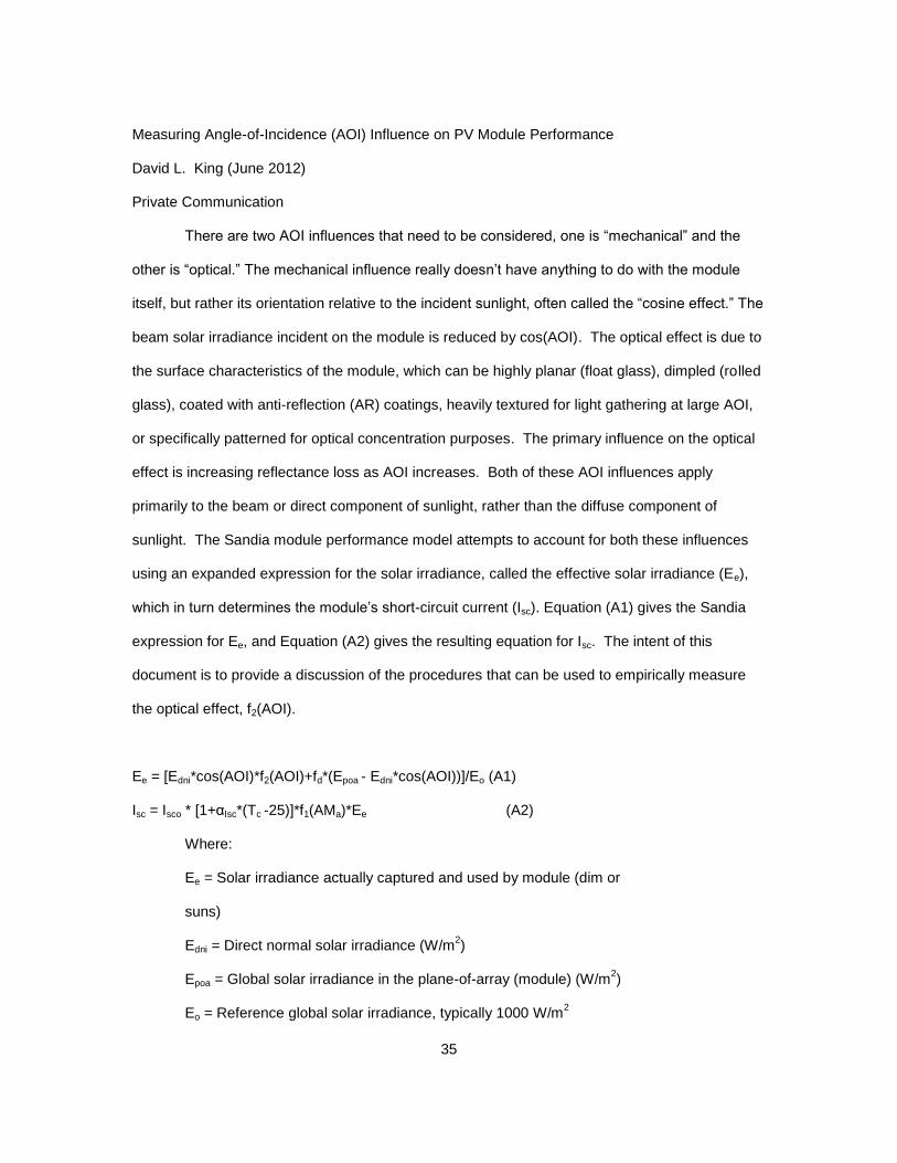
Measuring Angle-of-Incidence (AOI) Influence on PV Module Performance

David L. King (June 2012)

Private Communication

There are two AOI influences that need to be considered, one is “mechanical” and the

other is “optical.” The mechanical influence really doesn’t have anything to do with the module

itself, but rather its orientation relative to the incident sunlight, often called the “cosine effect.” The

beam solar irradiance incident on the module is reduced by cos(AOI). The optical effect is due to

the surface characteristics of the module, which can be highly planar (float glass), dimpled (rolled

glass), coated with anti-reflection (AR) coatings, heavily textured for light gathering at large AOI,

or specifically patterned for optical concentration purposes. The primary influence on the optical

effect is increasing reflectance loss as AOI increases. Both of these AOI influences apply

primarily to the beam or direct component of sunlight, rather than the diffuse component of

sunlight. The Sandia module performance model attempts to account for both these influences

using an expanded expression for the solar irradiance, called the effective solar irradiance (Ee),

which in turn determines the module’s short-circuit current (Isc). Equation (A1) gives the Sandia

expression for Ee, and Equation (A2) gives the resulting equation for Isc. The intent of this

document is to provide a discussion of the procedures that can be used to empirically measure

the optical effect, f2(AOI).

Ee = [Edni*cos(AOI)*f2(AOI)+fd*(Epoa - Edni*cos(AOI))]/Eo (A1)

Isc = Isco * [1+αIsc*(Tc -25)]*f1(AMa)*Ee (A2)

Where:

Ee = Solar irradiance actually captured and used by module (dim or

suns)

Edni = Direct normal solar irradiance (W/m2)

Epoa = Global solar irradiance in the plane-of-array (module) (W/m2)

Eo = Reference global solar irradiance, typically 1000 W/m2

36

fd = Fraction of diffuse irradiance used by module, typically

assumed = 1 (dim)

AOI = Angle between solar beam and module normal vector (deg)

Tc = Measured module (cell) temperature (°C)

αIsc = Short-circuit current temperature coefficient (1/°C)

f1(AMa) = Empirical relationship for solar spectral influence on Isc

versus air mass

Isco = Module short-circuit current at STC conditions (A)

Isc = Measured short-circuit current (A)

Direct Measurement of f2(AOI)

The direct procedure for measuring f2(AOI) involves measuring module Isc as the module

is moved in angular increments using a solar tracker through a wide range of AOI conditions, 0

deg to 90 deg. The challenge is to conduct the test in a way that either minimizes or

compensates for all the factors in Equations (A1) and (A2) that influence the measured Isc values.

The following bullets identify desirable conditions and approaches, depending on the capabilities

of the test equipment available.

Conduct test during clear sky conditions when the direct normal irradiance is the

dominant component, e.g. when the ratio of direct normal divided by global normal

irradiance is greater than about 0.85. This reduces the influence of diffuse irradiance on

the determination of f2(AOI).

Conducting the test near solar noon also has a couple advantages, variation in the solar

spectrum during the test is minimized, and the full range for AOI can typically be

achieved by changing only the elevation angle of a two-axis solar tracker.

Measure Isc, Edni, Epoa, and Tc associated with each AOI increment. Edni should be

measured with a thermopile pyrheliometer, and Epoa should ideally be measured using a

thermopile pyranometer that has been calibrated as a function of AOI.

37

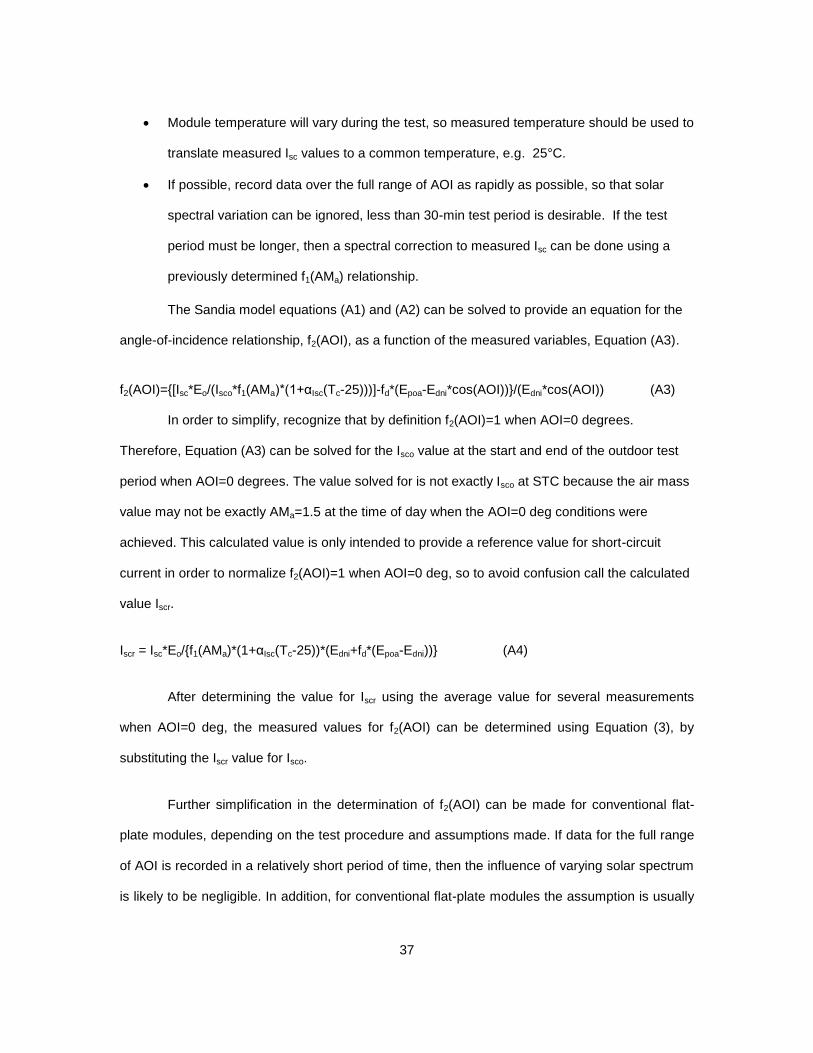
Module temperature will vary during the test, so measured temperature should be used to

translate measured Isc values to a common temperature, e.g. 25°C.

If possible, record data over the full range of AOI as rapidly as possible, so that solar

spectral variation can be ignored, less than 30-min test period is desirable. If the test

period must be longer, then a spectral correction to measured Isc can be done using a

previously determined f1(AMa) relationship.

The Sandia model equations (A1) and (A2) can be solved to provide an equation for the

angle-of-incidence relationship, f2(AOI), as a function of the measured variables, Equation (A3).

f2(AOI)={[Isc*Eo/(Isco*f1(AMa)*(1+αIsc(Tc-25)))]-fd*(Epoa-Edni*cos(AOI))}/(Edni*cos(AOI)) (A3)

In order to simplify, recognize that by definition f2(AOI)=1 when AOI=0 degrees.

Therefore, Equation (A3) can be solved for the Isco value at the start and end of the outdoor test

period when AOI=0 degrees. The value solved for is not exactly Isco at STC because the air mass

value may not be exactly AMa=1.5 at the time of day when the AOI=0 deg conditions were

achieved. This calculated value is only intended to provide a reference value for short-circuit

current in order to normalize f2(AOI)=1 when AOI=0 deg, so to avoid confusion call the calculated

value Iscr.

Iscr = Isc*Eo/{f1(AMa)*(1+αIsc(Tc-25))*(Edni+fd*(Epoa-Edni))} (A4)

After determining the value for Iscr using the average value for several measurements

when AOI=0 deg, the measured values for f2(AOI) can be determined using Equation (3), by

substituting the Iscr value for Isco.

Further simplification in the determination of f2(AOI) can be made for conventional flat-

plate modules, depending on the test procedure and assumptions made. If data for the full range

of AOI is recorded in a relatively short period of time, then the influence of varying solar spectrum

is likely to be negligible. In addition, for conventional flat-plate modules the assumption is usually

38

made that they capture both diffuse and direct irradiance; therefore fd=1. Under these simplified

conditions, Equations (A3) and (A4) can be rewritten as Equations (A5) and (A6).

Iscr = Isc*(Eo/Epoa)*(1+αIsc(Tc-25)) (A5)

f2(AOI) = [Eo* (Isc/(1+αIsc(Tc-25)))/Iscr -(Epoa-Edni*cos(AOI))]/(Edni*cos(AOI)) (A6)

For conventional flat-plate glass modules, this procedure should result in empirical

f2(AOI) relationships similar to those shown in Figure A1. As previously mentioned, AR-coated

glass or heavily textured glass will provide different results. For the simple case with a planar

glass surface, Snell’s and Bougher’s optic laws along with glass optical properties (index of

refraction, extinction coefficient, thickness) can also be used to calculate a theoretical relationship

for f2(AOI), as done by DeSoto in Reference [1].

Figure A 1: Empirical f2(AOI) measurements by Sandia National Laboratories for conventional flat-plate modules with a planar glass front surfaces.

Although polynomial fits to measured data can be problematic, ten years ago when the

procedure was developed and the Sandia module database initiated, a fifth order fit was used to

represent the measured data and reduce measured data problems. The “generic” polynomial

used for the majority of typical glass-surface modules is given below.

0.2

0.3

0.4

0.5

0.6

0.7

0.8

0.9

1.0

1.1

0 10 20 30 40 50 60 70 80 90

Angle-of-Incidence, AOI (deg)

Re

lati

ve

Re

sp

on

se

, f 2

(AO

I)

Glass, mc-Si

Glass, mc-Si

Glass, c-Si

Glass, a-Si

39

f2(AOI) = 1-2.4377E-3(AOI)+3.1032E-4(AOI)2-1.2458E-5(AOI)

3+2.1122E-7(AOI)

4-1.3593E-

9(AOI)5

Relative (Comparison) Measurements for f2(AOI)

Although not presented in this document, an alternative test procedure providing

simultaneous measurements of the Isc of a test module and a reference module may possibly

provide a more accurate and repeatable process. The reference module is assumed to have

“known f2(AOI)” characteristics. The reference device could be a module or an individual

reference cell, ideally with matching cell technology to provide equivalent solar spectral

sensitivity. For a reference device with ideally planar glass surface, the “known f2(AOI)” could be

derived from optical laws, perhaps providing a more fundamental basis for the outdoor test

procedure.

References

[1] W. DeSoto, S.A. Klein, W.A. Beckman, “Improvement and Validation of a Model for

Photovoltaic Array Performance,” Solar Energy, August 2005.

40

APPENDIX B

CROSSCHECKING OF AOI DEVICE USING MANUAL METHOD

41

In this study, the AOI was directly determined using an AOI device purchased from

MicroStrain. However, in the absence of this device, the AOI value can also be determined using

a manual calculation (equation B1) given by Sandia National Laboratories2.

(B1)

Where:

AOI = solar angle of incidence (degrees)

Tm = tilt angle of module (degrees, 0° is horizontal)

Zs = zenith angle of the sun (degrees)

AZm = azimuth angle of module (0°=North, 90°=East)

AZs = azimuth angle of sun (degrees)

As shown in Figure B1 (azimuth rotation) and Figure 1B (elevation rotation) below, the

accuracy of the AOI device used in this project was crosschecked with the manual method using

equation 1 given above. These plots confirm that the AOI data obtained using the MicroStrain

device was reliable and accurate. For azimuth angle, the tracker was allowed to rotate to its full

Westward rotation angle and tracked azimuthally to the East. The azimuth angle of the module

was manually measured by dividing the diameter of the tracker pole into 360° and fixing a dial to

the rotating head of the tracker to indicate its change in angle. Since the azimuthal rotation of the

tracker was limited, azimuth verification could only be obtained for AOI up to 63°.

42

Figure B 1: Comparison of relative optical responses obtained using the AOI hardware and AOI calculation for a CdTe module with glass superstrate for azimuth rotation(direct to global ratio was 0.89)

Figure B 2: Comparison of relative optical responses obtained using the AOI hardware and AOI calculation for a CdTe module with glass superstrate for elevation rotation (direct to global ratio was 0.89)

For elevation angle, the two-axis tracker was tilted to the maximum horizontal position of

11° (where 0° is horizontal) and tilted downward to a maximum angle of 74.5°. the f2(AOI) data

0

0.2

0.4

0.6

0.8

1

1.2

0 20 40 60 80 100

f 2(A

OI)

AOI (degrees)

AOI Measured with AOI Device

AOI Measured Manually

0

0.2

0.4

0.6

0.8

1

1.2

0 20 40 60 80 100

f2(A

OI)

AOI (degrees)

CdTe AOI Device

CdTe Manual AOI

Poly. (Sandia Polynomial)

43

for elevation angle deviates from the generalized polynomial for higher tilt angles due to the

inconsistent reflectance throughout the measurement. When the modules are at 11° tilt (close to

horizontal), they ‘see’ only the sky. As they are tilted downward, the ground reflection could

interfere with the data accuracy. This phenomenon does not occur for azimuth angles because

the modules are essentially seeing the same ratio of sky and ground (they were at 30° tilt angle

for the duration of the azimuth rotation).

The purpose of this experiment was to verify that the manual method and AOI device

measurements were consistent. Both methods proved to be accurate. The standard deviation

between manually calculated AOI and the AOI device measurement for azimuth angle was 1.66°.

The standard deviation between manually calculated AOI and AOI device measurement for

elevation tilt was 1.08°.

44

APPENDIX C

ROUND 1: MEASUREMENTS USING A MULTI-CURVE TRACER

45

The data presented in the main body (round 3; final round) of the report evolved from

previous two rounds of data collections and reductions. Improvements to the experimental setup

and data processing were made for each round. For round 1 of data collection, a DayStar

(DS3200) multi-curve tracer was used to measure and record Isc, module temperature, and

irradiance sensor readings. The main problems concerning round 1 measurements were:

1. The fastest time the multi-curve tracer could record and store data was one minute

intervals. This was due to a software limitation of the multi-curve tracer, not a hardware

issue. The multi-curve tracer saves data files onto the hard drive by automatically

assigning them a file name based on the time the data was collected. The data file is

named only for the hour and minute it is stored (not for the second). The physical

capabilities of the tracker allow it to take data for the five modules in ten seconds.

However, since the files are automatically assigned a name based on the time they were

taken, the minimum time interval the data could be recorded and stored was one minute.

For this experiment, the tracker was rotated by 5° AOI every one minute until it reached a

maximum of 77° AOI. The experiment was performed in 16 minutes and a total of 16

data points were collected. The 16 data points in 16 minutes is sufficient to comply with

the IEC 61853-2 standard which states for devices with rotational symmetry of the

reflectivity with respect to the module normal, do a minimum of 9 different angles to span

the angles from 0 to 80° for one direction. To confidently validate this statement, more

data points were needed. Since data should be recorded as quickly as possible to

reduce the spectral change during the experiment, round 2 was proposed to be carried

out using equipment that could measure and record data in less than one minute

intervals.

2. The irradiance sensors used for measuring global irradiance in the plane of array

(pyranometers) and direct normal irradiance (pyrheliometer) had not been calibrated, and

therefore, the accuracy of the measurements could not be confirmed and the uncertainty

could not be calculated.

46

The relative Isc obtained versus AOI plot is shown in Figure C1. Using Equation A6 of

Sandia, the relative optical response data, f2(AOI) data, was plotted (symbol) versus AOI as

shown in Figure C2. The plotted data (symbols) was then compared to the “generic” polynomial

curve (solid line) empirically derived by Sandia National Laboratories. As can be seen in this

figure, there is a significant difference between the f2(AOI) data calculated using the experimental

data and the generic polynomial curve (between 60o and 75

o). This difference warranted further

investigation. A further investigation revealed a human error that was made in constructing the

Equation A6 in the Excel spreadsheet. This error was fixed in the final rounds of data processing.

Nevertheless, the multi-curve tracer method, as opposed to the transducer/data logger method,

was not continued for the second and final rounds of measurements due to the limitation on the

number of data points that could be collected during the short duration of tracker rotation.

Figure C 1: Round 1 – Relative short circuit current verses

AOI for five modules (Multi-curve

tracer method)

0.0

0.2

0.4

0.6

0.8

1.0

1.2

0 20 40 60 80 100

Re

lati

ve

Isc

Angle of Incidence, AOI (degrees)

Poly-Crystalline Silicon

Mono-Crystalline Silicon A-Silicon

Drop in Isc value due to slight irradiance change probably due to thin passing cloud

47

Figure C 2: Round 1 - Data for five modules where f2(AOI) was erroneously calculated using Equation A6 (Multi-curve tracer method)

0

0.2

0.4

0.6

0.8

1

1.2

0 20 40 60 80 100

Re

lati

ve

Op

tica

l R

esp

on

ce,

f 2(A

OI)

)

Angle of Incidence, AOI (deg)

Poly-Crystalline Silicon

Mono-Crystalline Silicon

A-Silicon

CdTe

CIGS

Poly. (Sandia Generalized Polynomial)

48

APPENDIX D

ROUND 2: MEASUREMENTS USING A TRANSDUCERS AND DATA LOGGER

49

The second round of measurement involved the use of CR-magnetic DC transducers and

a Campbell scientific CR1000 data logger and multiplexer to measure and collect data for short

circuit current , module temperature, and reference cell . Few problems that were detected in the

round 1 of measurements were rectified in round 2 and they are as follows:

1) Multi-curve tracer was able to collect and store data for every one minute but in round 2,

the data logger and multiplexer were able to take and store data for every 30 seconds. In

round 2, 16 data points were collected in approximately 9.5 minutes.

2) The human error that was present in the MS Excel spreadsheet equation in round 1 was

corrected in round 2 and all the plots obtained from round 2 used the correct equation.

However, the reference devices were still not calibrated for the experiment, causing a

delay in calculating the uncertainty.

Figure D 1: Round 2 – Relative short circuit current verses AOI for five modules (Data logger method)

0

0.2

0.4

0.6

0.8

1

1.2

0 20 40 60 80 100

Re

lati

ve Is

c

Angle of Incidence, AOI (degrees)

Poly-Crystalline Silicon Mono-Crystalline Silicon A-Silicon

CdTe

CIGS Isc remains constant after 80° AOI due to the influence of diffuse irradiance component of sunlight

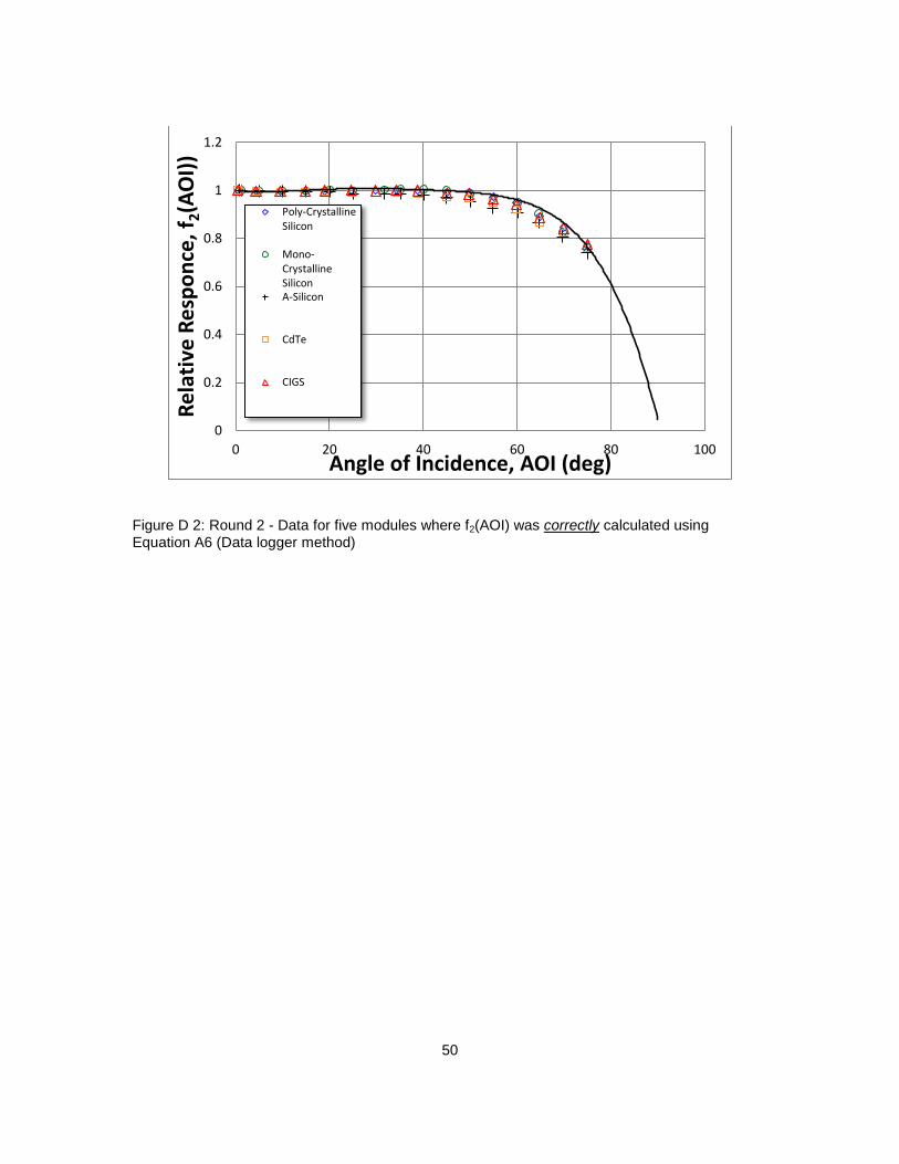
50

Figure D 2: Round 2 - Data for five modules where f2(AOI) was correctly calculated using Equation A6 (Data logger method)

0

0.2

0.4

0.6

0.8

1

1.2

0 20 40 60 80 100

Re

lati

ve R

esp

on

ce, f

2(A

OI)

)

Angle of Incidence, AOI (deg)

Poly-Crystalline Silicon

Mono-Crystalline Silicon A-Silicon

CdTe

CIGS

51

APPENDIX E

INTER-COMPARISON AND CROSSCHECKING OF PYRANOMETERS

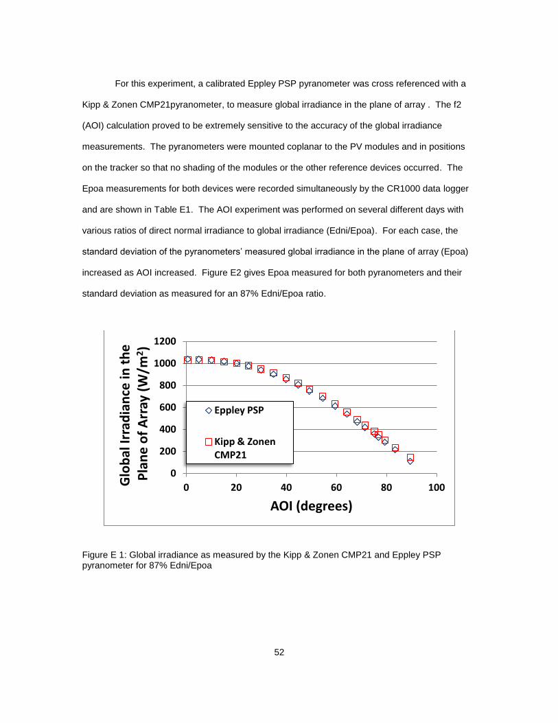
52

For this experiment, a calibrated Eppley PSP pyranometer was cross referenced with a

Kipp & Zonen CMP21pyranometer, to measure global irradiance in the plane of array . The f2

(AOI) calculation proved to be extremely sensitive to the accuracy of the global irradiance

measurements. The pyranometers were mounted coplanar to the PV modules and in positions

on the tracker so that no shading of the modules or the other reference devices occurred. The

Epoa measurements for both devices were recorded simultaneously by the CR1000 data logger

and are shown in Table E1. The AOI experiment was performed on several different days with

various ratios of direct normal irradiance to global irradiance (Edni/Epoa). For each case, the

standard deviation of the pyranometers’ measured global irradiance in the plane of array (Epoa)

increased as AOI increased. Figure E2 gives Epoa measured for both pyranometers and their

standard deviation as measured for an 87% Edni/Epoa ratio.

Figure E 1: Global irradiance as measured by the Kipp & Zonen CMP21 and Eppley PSP pyranometer for 87% Edni/Epoa

0

200

400

600

800

1000

1200

0 20 40 60 80 100 Glo

bal

Irra

dia

nce

in t

he

P

lan

e o

f A

rray

(W

/m2)

AOI (degrees)

Eppley PSP

Kipp & Zonen CMP21

53

Table E 1: Comparison of Kipp & Zonen CMP21 verses Eppley PSP measured global irradiance in the plane of array for 87% direct to global irradiance ratio

88% Edni to Epoa Ratio

AOI (degrees)

Kipp & Zonen Epoa

(W/m2)

Eppley Epoa

(W/m2)

Difference

(%)

0.6 1029.3 1038.6 0.9%

5.1 1030.3 1036.4 0.6%

10.1 1026.0 1029.5 0.3%

15.1 1015.2 1018.2 0.3%

20.2 1000.0 1000.0 0.0%

24.9 979.4 976.1 0.3%

29.8 949.1 940.9 0.9%

34.9 913.3 901.5 1.3%

39.9 868.9 854.4 1.7%

44.8 819.7 804.4 1.9%

49.2 764.8 747.8 2.3%

54.5 700.4 681.5 2.8%

59.5 629.9 610.2 3.2%

64.2 559.0 537.4 4.0%

68.3 489.3 468.4 4.5%

71.4 437.2 418.3 4.5%

75.2 381.8 359.9 6.1%

76.8 351.1 329.2 6.7%

79.4 302.6 282.5 7.1%

83.5 233.9 215.8 8.4%

89.6 146.0 109.2 33.7%

54

The data presented above represents the data used in the main body of this report.

However, experiments were also performed for other days with various direct to global irradiance

ratios. Figure E3 gives a comparison of irradiance data for a direct to global irradiance ratio of

81%. This data also shows a higher standard deviation for higher AOI. For AOI from 0° to 66°

the average standard deviation is 4% whereas for AOI from 67° to 90° the average standard

deviation is 15%. Figure E5 gives a comparison of irradiance data for an overcast day where the

ratio of direct to global irradiance was 2%. For this data, the standard deviation between the two

pyranometers remained approximately constant, but higher, for all AOI.

Figure E 2: Comparison of Kipp & Zonen CMP21 verses Eppley PSP measured global irradiance in the plane of array for 81% direct to global irradiance ratio

0

200

400

600

800

1000

1200

0 20 40 60 80 100

Glo

bal

Irra

dia

nce

in t

he

P

lan

e o

f A

rray

(W

/m2)

AOI (degrees)

Eppley PSP

Kipp & Zonen CMP21

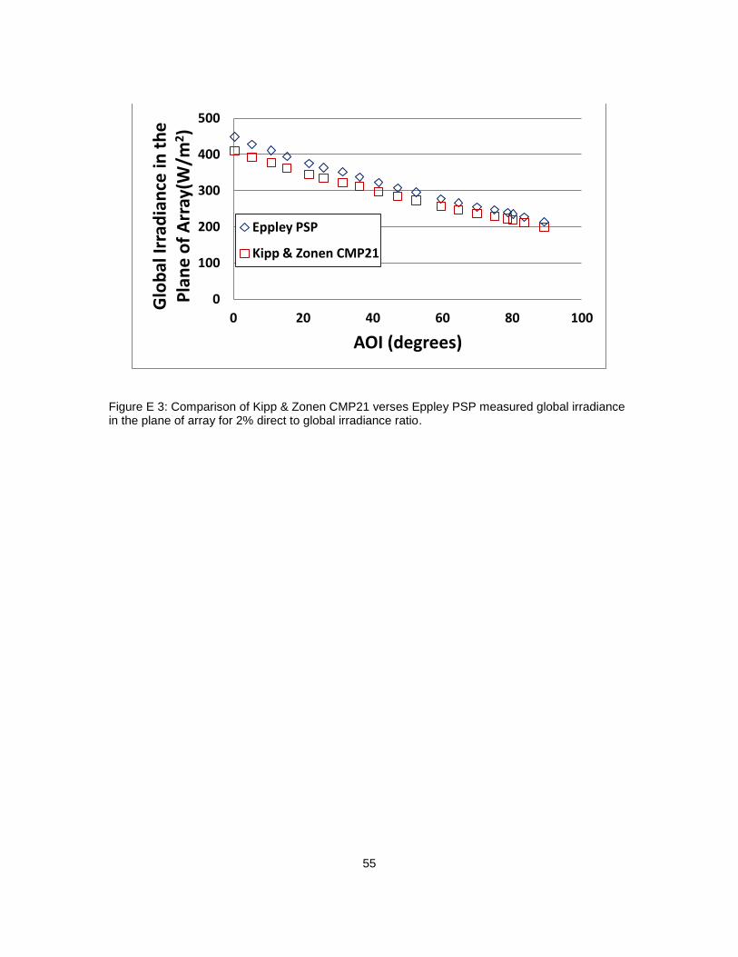
55

Figure E 3: Comparison of Kipp & Zonen CMP21 verses Eppley PSP measured global irradiance in the plane of array for 2% direct to global irradiance ratio.

0

100

200

300

400

500

0 20 40 60 80 100

Glo

bal

Irra

dia

nce

in t

he

P

lan

e o

f A

rray

(W/m

2)

AOI (degrees)

Eppley PSP

Kipp & Zonen CMP21

56

APPENDIX F

MEASUREMENT OF f2(AOI) VERSES AOI IN THE OPPOSITE DIRECTION

57

Standard IEC 61853-2 (draft) called for the verification of rotational symmetry of the

reflectivity with respect to the module normal. First, the data was collected by rotating the tracker

from west (starting at 0.59o AOI) to the east (ending at 83.50

o) within ten minutes. Then the

tracker was set to automatic mode and was tracking from east to west. By using the Sandia

equation A6 a graph was plotted as shown in Figure F1.

Figure F 1: Round 3 - Data for five modules where f2(AOI) was calculated when the tracker was rotated in the opposite direction (East to West)

There were a few disadvantages noted while allowing the tracker to track in the automatic

mode. While doing the test in the manual mode, the tracker was rotated both in azimuth and

elevation proportionally. When the tracker is allowed to track back, the elevation angle is

adjusted first and then rotates in the azimuth. However, the relative optical response of the

module is not affected. The AOI changes faster when the tracker is tilted in the elevation than

rotating the tracker azimuthally. Since the tracker was rotated in the elevation for the first 30

seconds, the AOI of 83o at 14:37:30 and 63

o at 14:38:00 were able to be recorded. After

adjusting for the elevation, the tracker was able to rotate azimuthally and hence more data points

were able to be collected.

0

0.2

0.4

0.6

0.8

1

1.2

0 20 40 60 80 100 Re

lati

ve O

pti

cal R

esp

on

se

f2(A

OI)

AOI (degrees)

CdTe

A-Si

CIGS

Mono-Si

58

Figure F 2: Round 3 - Data for f2(AOI) calculated for CdTe from West to East compared to data when the tracker was rotated in the opposite direction (East to West)

Figure F 3: Round 3 - Data for f2(AOI) calculated for a-Si from West to East compared to data when the tracker was rotated in the opposite direction (East to West)

0

0.2

0.4

0.6

0.8

1

1.2

0 20 40 60 80 100

Re

lati

ve O

pti

cal R

esp

on

se

f2(A

OI)

AOI (degrees)

CdTe (East to West)

CdTe (West to East)

0

0.2

0.4

0.6

0.8

1

1.2

0 20 40 60 80 100

Re

lati

ve O

pti

cal R

esp

on

se

f2(A

OI)

AOI (degrees)

A-Si (East to West)

A-Si (West to East)

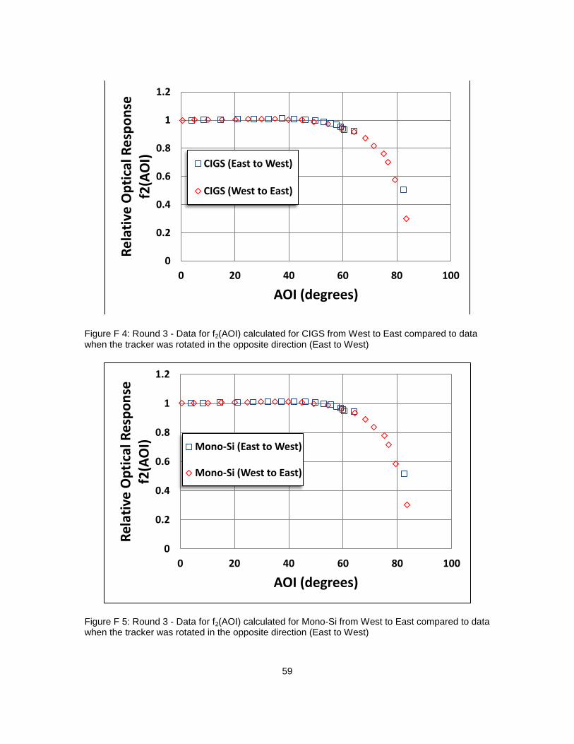
59

Figure F 4: Round 3 - Data for f2(AOI) calculated for CIGS from West to East compared to data when the tracker was rotated in the opposite direction (East to West)

Figure F 5: Round 3 - Data for f2(AOI) calculated for Mono-Si from West to East compared to data when the tracker was rotated in the opposite direction (East to West)

0

0.2

0.4

0.6

0.8

1

1.2

0 20 40 60 80 100

Re

lati

ve O

pti

cal R

esp

on

se

f2(A

OI)

AOI (degrees)

CIGS (East to West)

CIGS (West to East)

0

0.2

0.4

0.6

0.8

1

1.2

0 20 40 60 80 100

Re

lati

ve O

pti

cal R

esp

on

se

f2(A

OI)

AOI (degrees)

Mono-Si (East to West)

Mono-Si (West to East)

60

Figure F 6: Round 3 - Data for f2(AOI) calculated for Poly-Si from West to East compared to data when the tracker was rotated in the opposite direction (East to West)

0

0.2

0.4

0.6

0.8

1

1.2

0 20 40 60 80 100

Re

lati

ve O

pti

cal R

esp

on

se

f2(A

OI)

AOI (degrees)

Poly-Si (East to West)

Poly-Si (West to East)

61

APPENDIX G

GRAPHICAL METHOD FOR FINDING THE PARAMETER CAUSING DROP IN POWER

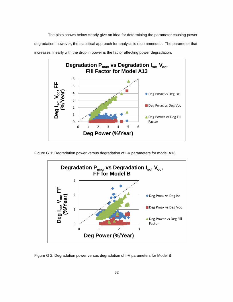
62

The plots shown below clearly give an idea for determining the parameter causing power

degradation, however, the statistical approach for analysis is recommended. The parameter that

increases linearly with the drop in power is the factor affecting power degradation.

Figure G 1: Degradation power versus degradation of I-V parameters for model A13

Figure G 2: Degradation power versus degradation of I-V parameters for Model B

0

1

2

3

4

5

6

0 1 2 3 4 5 6

De

g I

sc, V

oc, F

F

(%

/Ye

ar)

Deg Power (%/Year)

Degradation Pmax vs Degradation Isc, Voc, Fill Factor for Model A13

Deg Pmax vs Deg Isc

Deg Pmax vs Deg Voc

Deg Power vs Deg Fill Factor

0

1

2

3

0 1 2 3

De

g I

sc, V

oc, F

F

(%

/Ye

ar)

Deg Power (%/Year)

Degradation Pmax vs Degradation Isc, Voc, FF for Model B

Deg Pmax vs Deg Isc

Deg Pmax vs Deg Voc

Deg Power vs Deg Fill Factor

63

Figure G 3: Degradation power versus degradation of I-V parameters for model C12

Figure G 4: Degradation power versus degradation of I-V parameters for Model C4

0

1

2

3

4

5

0 1 2 3 4 5 6 7 8

De

g I

sc, V

oc, F

F

(%

/Ye

ar)

Deg Power (%/Year)

Degradation Pmax vs Degradation Isc, Voc, FF for Model C12

Deg Power vs Deg Isc

Deg Power vs Deg Voc

0

1

2

3

4

5

6

0 1 2 3 4 5 6

De

g I

sc,V

oc,F

F

(%

/Ye

ar)

Deg Power (%/Year)

Degradation Pmax vs Degradation Isc, Voc, FF for Model C4

Deg Power vs Deg Isc

Deg Power vs Deg Voc

Deg power vs Deg Fill Factor

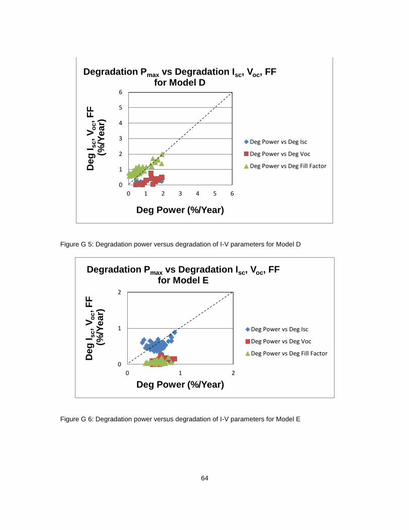
64

Figure G 5: Degradation power versus degradation of I-V parameters for Model D

Figure G 6: Degradation power versus degradation of I-V parameters for Model E

0

1

2

3

4

5

6

0 1 2 3 4 5 6

De

g I

sc, V

oc, F

F

(%

/Ye

ar)

Deg Power (%/Year)

Degradation Pmax vs Degradation Isc, Voc, FF for Model D

Deg Power vs Deg Isc

Deg Power vs Deg Voc

Deg Power vs Deg Fill Factor

0

1

2

0 1 2

De

g I

sc, V

oc, F

F

(%

/Ye

ar)

Deg Power (%/Year)

Degradation Pmax vs Degradation Isc, Voc, FF for Model E

Deg Power vs Deg Isc

Deg Power vs Deg Voc

Deg Power vs Deg Fill Factor

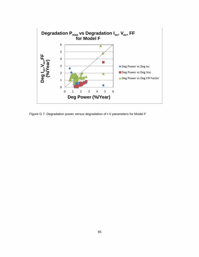
65

Figure G 7: Degradation power versus degradation of I-V parameters for Model F

0

1

2

3

4

5

6

0 1 2 3 4 5 6

De

g I

sc,V

oc,F

F

(%/Y

ea

r)

Deg Power (%/Year)

Degradation Pmax vs Degradation Isc, Voc, FF for Model F

Deg Power vs Deg Isc

Deg Power vs Deg Voc

Deg Power vs Deg Fill Factor

66

APPENDIX H

PARETO CHART OF DEFECTS IN MODULES FOR EACH TYPE OF MODEL

67

In order to find the primary visual defect that accounts for the drop in power, visual

inspection data for each model was obtained from previous researcher’s database and was

constructed as a Pareto chart in Minitab software. The Pareto chart is a pictorial representation

giving the frequency and percentage of occurrence of an observation. The Pareto chart of

defects for each type of model is given below.

Figure H 1: Pareto chart of defects for Model A13

Figure H 2: Pareto chart of defects for Model B

Count 168 168 168

Percent 33.3 33.3 33.3

Cum % 33.3 66.7 100.0

Rear Sea

l Dete

riora

tion

Front

Seal

Det

eriora

tion

Disco

lora

tion O

f Enca

psula

nt

500

400

300

200

100

0

100

80

60

40

20

0

Co

un

t

Pe

rce

nt

Pareto Chart of defect for Model A-13

Count 1153 630 8 4 1

Percent 64.2 35.1 0.4 0.2 0.1

Cum % 64.2 99.3 99.7 99.9 100.0

Solder M

elted

Delam

inat

ion

Hotsp

ots w

ith IR

Camera

Minor S

ubstra

te W

arping

Discol

oratio

n of E

ncaps

ulant

2000

1500

1000

500

0

100

80

60

40

20

0

Co

un

t

Pe

rce

nt

Pareto Chart of defects of Model B

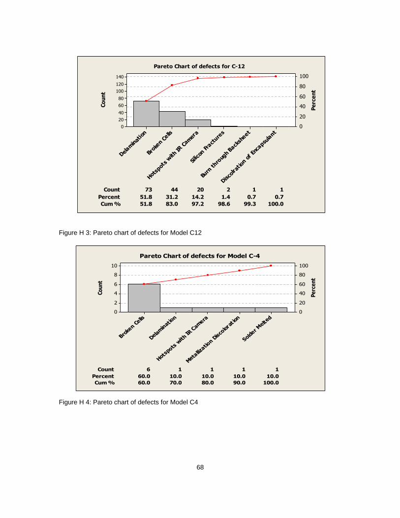
68

Figure H 3: Pareto chart of defects for Model C12

Figure H 4: Pareto chart of defects for Model C4

Count 73 44 20 2 1 1

Percent 51.8 31.2 14.2 1.4 0.7 0.7

Cum % 51.8 83.0 97.2 98.6 99.3 100.0

Disco

lrat io

n of En

capsu

lant

Burn

thro

ugh B

acksh

eet

Silic

on Fra

cture

s

Hots

pots w

ith IR

Cam

era

Broke

n Cells

Delam

inat

ion

140

120

100

80

60

40

20

0

100

80

60

40

20

0

Co

un

t

Pe

rce

nt

Pareto Chart of defects for C-12

Count 6 1 1 1 1

Percent 60.0 10.0 10.0 10.0 10.0

Cum % 60.0 70.0 80.0 90.0 100.0

Solder

Melt

ed

Meta

llizatio

n Disco

lora

t ion

Hots

pots w

ith IR

Cam

era

Dela

min

ation

Broke

n Cells

10

8

6

4

2

0

100

80

60

40

20

0

Co

un

t

Pe

rce

nt

Pareto Chart of defects for Model C-4

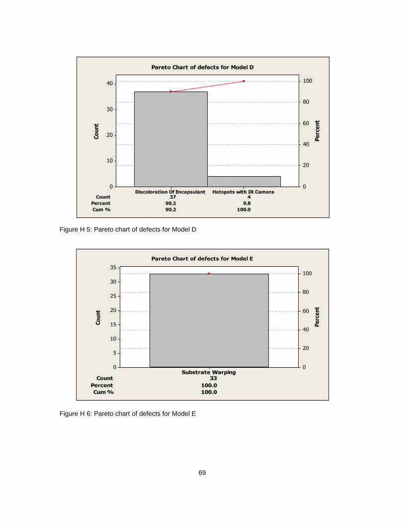
69

Figure H 5: Pareto chart of defects for Model D

Figure H 6: Pareto chart of defects for Model E

Count 37 4

Percent 90.2 9.8

Cum % 90.2 100.0

Hotspots with IR CameraDiscoloration Of Encapsulant

40

30

20

10

0

100

80

60

40

20

0

Co

un

t

Pe

rce

nt

Pareto Chart of defects for Model D

Count 33

Percent 100.0

Cum % 100.0

Substrate Warping

35

30

25

20

15

10

5

0

100

80

60

40

20

0

Co

un

t

Pe

rce

nt

Pareto Chart of defects for Model E

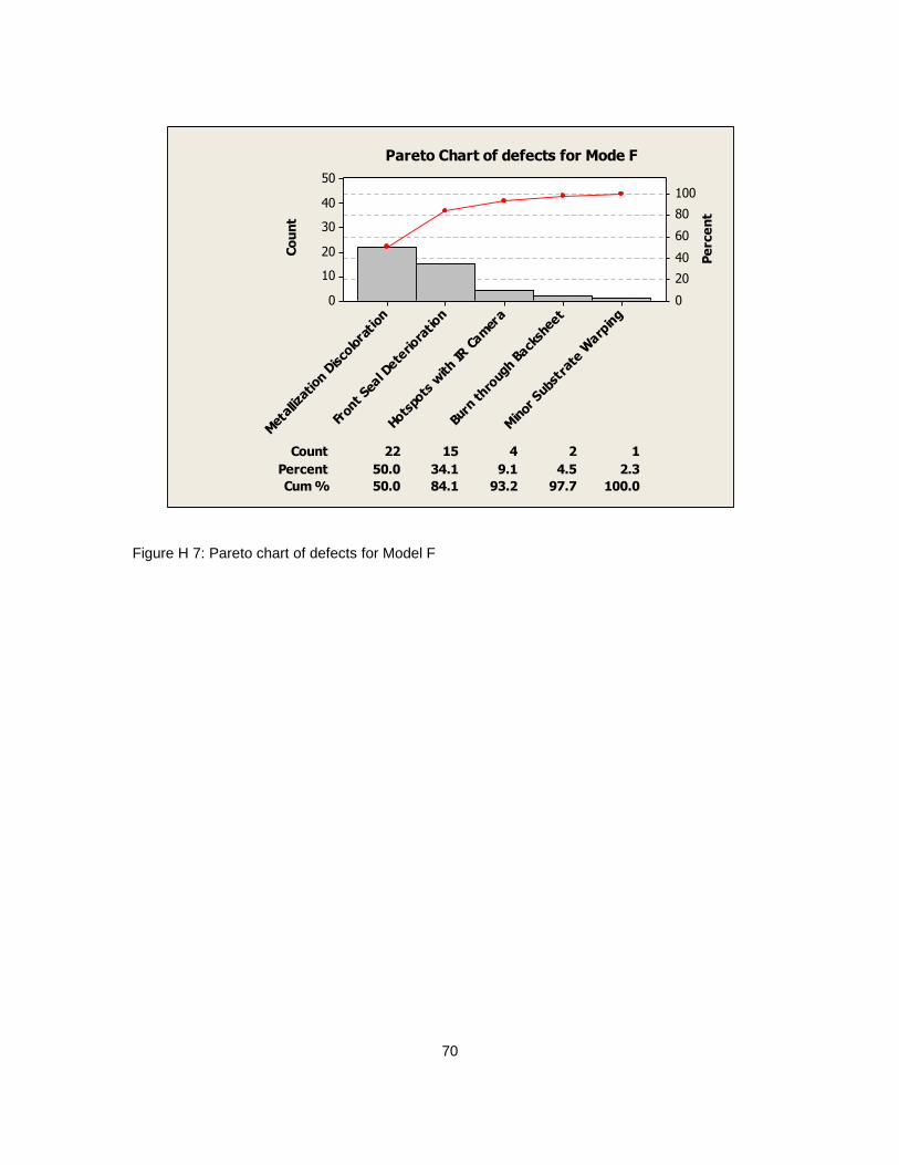
70

Figure H 7: Pareto chart of defects for Model F

Count 22 15 4 2 1

Percent 50.0 34.1 9.1 4.5 2.3

Cum % 50.0 84.1 93.2 97.7 100.0

Min

or S

ubstr

ate W

arpin

g

Burn

thro

ugh B

acksh

eet

Hotspo

ts w

ith IR

Cam

era

Fron

t Sea

l Dete

riora

tion

Meta

lliza

tion D

isco

lora

tion

50

40

30

20

10

0

100

80

60

40

20

0C

ou

nt

Pe

rce

nt

Pareto Chart of defects for Mode F

71

APPENDIX I

ANNUAL AVERAGE DEGRADATION RATE FOR I-V PARAMETERS FOR ALL MODELS

72

The plots for annual average degradation of I-V parameters for each model are shown as below.

Figure I 1: Plot for average annual degradation of I-V parameters for Model A13

Figure I 2: Plot for average annual degradation of I-V parameters for Model B

0

0.5

1

1.5

2

2.5

Ave

rag

e A

nn

ua

l D

eg

rad

ati

on

Ra

te

Parameter

Plot of Various Parameters vs Degradation Rate Per Year for

Model A13

A-13

-0.2

0

0.2

0.4

0.6

0.8

1

1.2

1.4

1.6

1.8

Ave

rag

e A

nn

ua

l D

eg

rad

ati

on

R

ate

Parameters

Plot of Various Parameters vs Degradation Rate Per Year for

Model B

B

Pmax Isc Voc FF Imp Vmp

Pmax Isc Voc FF Imp Vmp

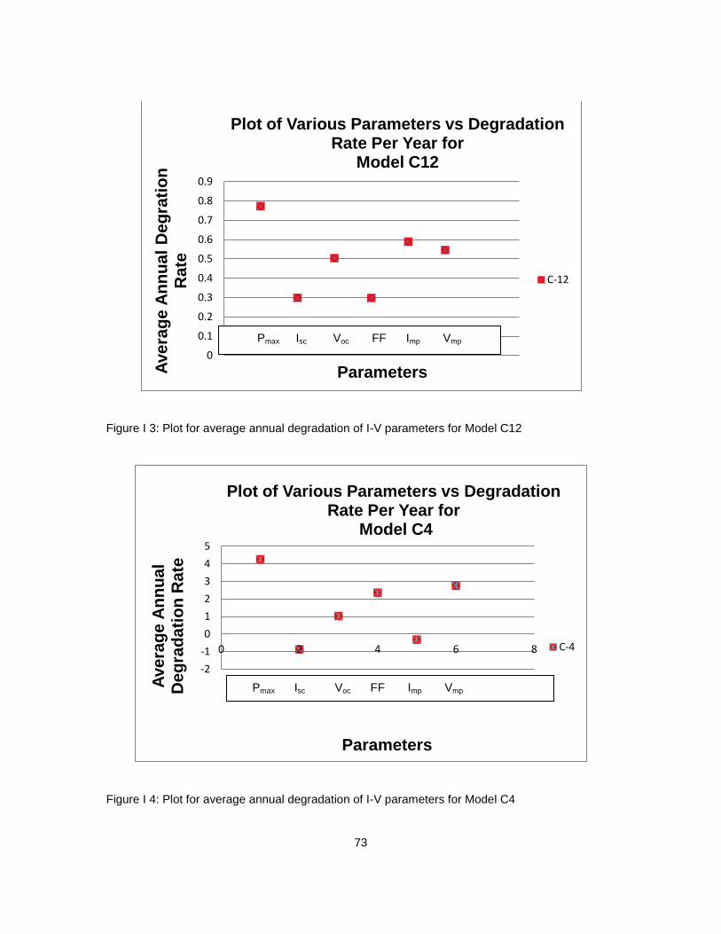
73

Figure I 3: Plot for average annual degradation of I-V parameters for Model C12

Figure I 4: Plot for average annual degradation of I-V parameters for Model C4

0

0.1

0.2

0.3

0.4

0.5

0.6

0.7

0.8

0.9

Ave

rag

e A

nn

ua

l D

eg

rati

on

R

ate

Parameters

Plot of Various Parameters vs Degradation Rate Per Year for

Model C12

C-12

-2

-1

0

1

2

3

4

5

0 2 4 6 8

Ave

rag

e A

nn

ua

l

De

gra

da

tio

n R

ate

Parameters

Plot of Various Parameters vs Degradation Rate Per Year for

Model C4

C-4

Pmax Isc Voc FF Imp Vmp

Pmax Isc Voc FF Imp Vmp

74

Figure I 5: Plot for average annual degradation of I-V parameters for Model D

Figure I 6: Plot for average annual degradation of I-V parameters for Model E

-0.8

-0.6

-0.4

-0.2

0

0.2

0.4

0.6

0.8

1

1.2

1.4

0 2 4 6 8

Ave

rag

e A

nn

ua

l D

eg

rad

ati

on

R

ate

Parameters

Plot of Various Parameters vs Degradation Rate Per Year for

Model D

D

-0.1

0

0.1

0.2

0.3

0.4

0.5

0.6

Avera

ge A

nn

ual

De

gra

da

tio

n R

ate

Parameters

Plot of Various Parameters vs Degradation Rate Per Year for

Model E

E

Pmax Isc Voc FF Imp Vmp

Pmax Isc Voc FF Imp Vmp

75

Figure I 7: Plot for average annual degradation of I-V parameters for Model F

-0.6 -0.4 -0.2

0 0.2 0.4 0.6 0.8

1 1.2 1.4 1.6

0 2 4 6 8 Ave

rag

e A

nn

ua

l D

eg

rad

ati

on

R

ate

Parameters

Plot of Various Parameters vs Degradation Rate Per Year for Model F

F

Pmax Isc Voc FF Imp Vmp

76

APPENDIX J

HISTOGRAMS OF POWER DEGRADATION FOR VARIOUS MODELS

77

The histograms of power degradation for the models in the power plant are as follows:

Figure J 1: Histogram of Power Degradation (%/Year) for Model A13

Figure J 2: Histogram of Power Degradation (%/Year) for Model B

78

Figure J 3: Histogram of Power Degradation (%/Year) for Model C12

Figure J 4: Histogram of Power Degradation (%/Year) for Model C4

79

Figure J 5: Histogram of Power Degradation (%/Year) for Model D

Figure J 6: Histogram of Power Degradation (%/Year) for Model E

80

Figure J 7: Histogram of Power Degradation (%/Year) for Model F

81

APPENDIX K

SAMPLE HYPOTHESIS TESTING USING MINITAB SOFTWARE

82

STEP 1: The null and alternative hypotheses are defined.

Null hypothesis: Degradation Isc/Year= Degradation FF/year

Alternative hypothesis: Degradation Isc/Year= Degradation Voc/Year

The degradation values of Isc, Voc and Fill Factor per year are collected for Model B

Figure K 1: Degradation values of Isc, Voc and Fill Factor per year pasted on Minitab Software Worksheet

STEP2:

Figure K 2: Options button for performing 2 Sample t test in Minitab

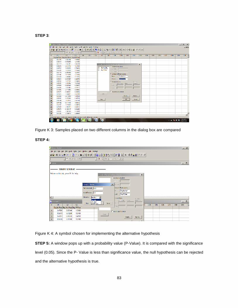
83

STEP 3:

Figure K 3: Samples placed on two different columns in the dialog box are compared

STEP 4:

Figure K 4: A symbol chosen for implementing the alternative hypothesis

STEP 5: A window pops up with a probability value (P-Value). It is compared with the significance

level (0.05). Since the P- Value is less than significance value, the null hypothesis can be rejected

and the alternative hypothesis is true.

84

Figure K 5: Window containing the P-Value

The same procedure is followed for implementing the hypothesis testing between

Degradation Isc per year and Degradation Voc per year and the statistical factor affecting the

power drop could be identified.

The entire procedure is followed for all models in the power plant to identify the major factor

causing the power drop.