AnEmpirical AnalysisofInformationally Restricted …...AnEmpirical AnalysisofInformationally...

An Empirical Analysis of Informationally RestrictedDynamic Auctions of Used Cars†

Sungjin ChoSeoul National University

Harry PaarschUniversity of Melbourne

John RustGeorgetown University

Preliminary, not for circulation

March, 2014

Abstract

We analyze a dynamic informationally restricted auction mechanism a rental car companycreated to sell its cars. All bids are submitted via the internet in continuous time in ascendingprice auctions that last for two minutes. Unlike English or Japanese auctions, bidders donot observe the number of other bidders in the auction or their bids. At any time in theauction each bidder only knows a) the history of their own bids, and b) whether or not theirbid is the current high bid. The bidder with the highest bid at the end of the auction is thewinner and pays their winning bid. We develop theoretical and empirical models of biddingstrategies in this auction and estimate bidders’ beliefs and distributions of valuations for usedcars. We show that there is a substantial amount of early bidding in these auctions, eventhough a game-theoretic analysis suggests that the informational restrictions should createstrong incentives for bid sniping — i.e. waiting to submit a bid only in the final second of theauction. If all bidders used non-informative bid sniping strategies the outcome of the auctionwould be equivalent to that of a static sealed bid auction. Bidders have an incentive to bidearly in the auction to learn what the current high bid is (since they learn this only if theirbid is the current high bid), but early bidding can operate to their collective disadvantage,leading them to bid more than they would in a static first price sealed bid auction. We useour model and estimated distribution of valuations for cars to compare auction revenues underthe dynamic auction with counterfactual revenues from a static sealed bid auction with andwithout a reservation price under the same informational restrictions (i.e. that bidders do notknow the number of competing bidders participating in any individual auction).

†Preliminary draft, not for quotation or public distribution. Direct comments to Sungjin Cho at Department of

Economics, Seoul National University, Seoul, Korea, email: [email protected].

1 Introduction

This paper provides an empirical analysis of a unique new dataset on auctions of individual cars by

a large rental car company. The rental company sells large numbers of used cars in a sequence of

auctions each month. These auctions are held on a secure website and are conducted sequentially,

with one car being sold in each auction. The participants in each auction are a self-selected

sample of professional bidders who choose to participate in each auction. There is population of

up to 90 professional bidders that include auto dealers and other intermediaries in the car market

who could potentially bid in any given auction. However an average of only 7 bidders actually

participate in a typical car auction.

The informationally restricted, ascending bid auctions designed by the rental company are

unlike other types of auctions that have been analyzed in the theoretical literature on auctions,

at least that we are aware of. The auctions are conducted electronically, over the Internet, and

proceed in continuous time, over two minute intervals. Bids typically increase in these auctions,

so they can be viewed as ascending auctions. However unlike the English auctions that are also

continuous time ascending auctions, the bidders in the rental car auctions are not able to observe

the number of other bidders or their bids. Instead, at any time each bidder knows only the history

of their own bids and whether or not their bid is the highest. The bidder with the highest bid at

the end of the two minute auction period wins the auction and their payment is the amount of

their winning bid. The only other auction that we are aware of that has informational restrictions

similar to the auction we analyze are auctions of certificates of deposit (CDs) conducted by

the state of Texas. In these auctions the bidders are banks and the “objects” being auctioned

are multiple unit parcels of loans in $100,000 increments. Groeger and Miller [2013] provide an

empirical analysis of this auction, under the assumption that bidding in the auction follows a

Perfect Bayesian Equilibrium (PBE).

We argue that calculating even a single PBE of this auction game is an incredibly complex

undertaking due to the high dimensionality of the posterior beliefs of bidders, assuming there

exists an informative equilibrium where bidders choose to place early bids in the auction. We

are presently able to analyze only the simplest case — a two player, two period bidding game

who have independent, uniformly distributed valuations. We show that there is no symmetric

1

informative equilibrium to this game, i.e. there is no equilibrium in which bidders submit non-

zero bids in the first stage of the auction and use the information from the outcome of the first

stage to condition their bids in the second stage. We show the early bidding operates to the

bidders’ disadvantage, because it results in an endogenously asymmetric auction equilibrium in

the second stage. Intelligent bidders realize this, and this is why they decide not to bid in the first

stage, and only submit bids in the second stage of the auction. The non-informative equilibrium

is equivalent to the Bayesian-Nash equilibrium of a single shot first price, sealed bid auction with

an unknown number of bidders participating. The non-informative equilibrium always exists, but

our example suggests that it is an open question whether informative PBE exist in this game. If

not, there is a puzzle since the early bidding we observe in these auctions is manifestly inconsistent

with the non-informative equilibrium where all bidders engage in bid-sniping, i.e. submitting their

bids only in the last second of the auction.

We present an alternative “behavioral” approach to the analysis of this new auction institution

and we structurally estimate the model using a data set of 11,790 individual used car auctions that

were conducted under this dynamic auction mechanism. Our dynamic model of bidding behavior

captures the main features of actual bidding behavior that we observe in our data set. Using

these data and this model we are able to obtain estimates of the distribution of bidder valuations

for individual cars offered for auction under an “independent private values” assumption that

bidder valuations are independent draws from a distribution centered on a “predicted fair market

value” for each used car, where this predicted fair market value is similar to the so-called “Blue

Book value” that is used as a starting point for valuing used cars in the United States. Using

these estimates, we are able to simulate bidder behavior under certain counterfactual auction

institutions, including the static optimal auction mechanism, which takes the form of a sealed

bid, second price auction with an appropriately determined reservation price, see Myerson [1981].

The rental car company claims that it designed its auctions in part to defeat collusion by

bidders. Prior to adoption of the online auction mechanism, the company used an ad hoc sell-

ing procedure to sell of its used cars, and this selling procedure frequently involved individu-

ally bargained prices, often negotiated with only a single interested buyer at a time. Cho et al.

[forthcoming, 2014] compare expected revenues from sales of used cars before and after the adop-

tion of the auction procedure and find that the adoption of the online auction mechanism signif-

2

icantly increased expected revenues from used car sales, and in particular, greatly reduced the

incidence of cars sold at prices far below their estimated fair market values. However the company

also sold many of its cars through a large auction house, which used a version of open-outcry En-

glish auction. Cho et al. [forthcoming, 2014] also found that the expected revenues from the Inter-

net auction were significantly less than the expected revenues the company earned in the English

auctions, a finding consistent with the prediction of the linkage principle of Milgrom and Weber

[1982].

Section 1 introduces the auction and the data used in our study. Section 2 discusses equilibrium

models of bidding in this auction and the difficulty of computing Perfect Bayesian Equlibrium

(PBE) solutions and the potential multiplicity of PBE. We show that there is no symmetric

informative PBE in a two period, two bidder example. Thus, it is an outstanding question

whether there exist informative asymmetric PBE to this game, or informative symmetric PBE in

games with more bidders and periods that results in behavior consistent with the early bidding

that we observe in these auctions. Section 3 introduces a behavioral model of bidding behavior in

the spirit of the oblivious equilibrium concept of Weintraub et al. [2008]. Section 4 econometrically

estimates the model and evaluates the fit of the model to the data and the implied estimates of

the distribution of valuations. Section 5 provides simulations of the expected revenues from the

company’s auction mechanism relative to the expected revenues from an optimal auction under

the hypothesis of independent private values and no bidder collusion. Section 6 provides some

concluding comments and suggestions for further research.

2 Auction Data

A large rental car company has generously provided us with data on auctions of all cars sold

under its new online auction system from 2005 to present. We have data on 11,701 individual

car auctions during this period. Unfortunately due to confidentiality restrictions we are unable

to provide further details on the company or its location.

The company uses the online auction mechanism it designed to sell large numbers of cars each

month in a sequence of back to back two minute auctions, where only a single car is sold in each

auction. Bidders have some advance notice of the auctions and the cars that are to be sold in

3

the auctions, and this allows them an opportunity to visit the company to physically inspect the

cars to be sold. Bidders do not undertake mechnical inspections, but rather a bidding agent does

a brief “walk around” to inspect the interior and exterior condition of the car, and can request a

copy of the vehicle’s maintenance history, including the total amount spent on maintenance, dates

of maintenance, records of accidents, and so forth. Our data includes the same maintenance and

accident records that were available to these bidders, but the information we do not have that

bidders do have is the information gained from the physical inspection and “walk around” of the

vehicle. We will account for this additional information that buyers have (and their potentially

heterogeneous evaluations of this information) in our empirical model in section 3.

The company starts the auctions of the lot of vehicles to be sold in the morning with no

pauses between auctions. As noted above, each auction lasts two minutes, and our data includes

time stamps and the amounts of each bid and the identities of each bidder in each auction. Some

time stamps are a few milliseconds past the two minute auction closing time, but in general,

we excluded auctions took longer than 121 seconds as many of these auctions reflected special

circumstances (such as technical problems with the auction server) that required extra time to

complete the auction.1 In all instances, these slightly late bids were allowed as valid bids in the

auction. Up to 200 cars are auctioned on a particular day, and the company frequently auctions

cars on two successive days in each month in order to sell off all the cars it wishes to sell during

that month. There is no reservation price for the auctions and in virtually every auction, the

company sold the car to the highest bidder in each auction, regardless of the value of the winning

bid. The only exceptions we are aware of are a small number of auctions where a bidder made a

data entry error, keying in a bid that is far in excess of any reasonable value for the car. In such

cases, the company cancelled the auction outcome as invalid and re-auctioned the car at a later

date.

Figure 1 plots the data for auction 1 held on January 26, 2005. This was the first auction that

was held on this particular day. A four door mid-sized sedan was sold in this auction: we have

more precise details on the exact make and model but for purposes of this explanation it suffices

to mention that the car was about two years old with approximately 40,000 miles on its odometer

1Some auctions lasted 10 minutes but we do not know if there was some technical problem during these auctionsthat cause the company to extend the usual 2 minute duration, or whether there is some other reason for having alonger than usual duration. Overall we excluded 198 auctions whose total duration exceeded 121 seconds.

4

at the time of sale.

As we can see from the figure, there were six different bidders participating in this auction.

We also see that the bids are generally montonically increasing, though not all bidders are active

at every possible instant. The winning bidder in this auction, B41, delayed submitting its bid

until there were approximately 50 seconds remaining in this two minute auction, and it made only

one further revision to its first bid, raising it from $5000 to approximately $5400 at the very last

instant of the two minute auction.

On the other hand, we see an interesting range in bidding behavior for the other bidders.

Some bidders posted bids much earlier in the auction and made frequent changes to their bids.

These bidders appeared to be attempting to “probe” or “test” the market to find the smallest

bid they could make that would make them the highest bidder. They did this by making small

and frequent increases in their bids as in the case of B5. However B5 never succeeded in placing

a highest bid, and so only learned at most that the high bid was higher than each of its sucessive

bids, with the last bid reaching just over $4500 with less than 30 seconds remaining in the auction,

after which this bidder appeared to have given up and declined to submit any further bids. In all

likelihood this bidder had a reservation price for the vehicle and was unwilling to bid above this

reservation value, so its final bid could be a good signal of this reservation value (i.e. the highest

amount it would be willing to bid for the vehicle in the auction).

Figure 2 plots another auction where there are 7 participating bidders and a different firm

won the auction, B36. This bidder behaved differently than the winning bidder in auction 1 (B41)

by virtue of being the first bidder to place a bid in the auction, with a bid of $4000 just seconds

after the start of the auction, and then consistently increasing its bid in a series of small steps

over nearly the entire duration of the auction until it placed the winning bid of approximately

$7100 in the final instant of the auction. B36 and B41 appear to be “dueling” with each other

to maintain the highest bid, though neither used the strategy of jump bidding to try to win. B41

did delay placing its first bid until approximately the last 30 seconds of the auction, and its first

bid was higher, $6000. But in this auction, unlike in auction 1, B41 did increase its subsequent

bids in small increments while it appeared to be dueling with B36 to maintain the high bid, and

both B41 and B36 placed bids in the very last instant of the auction, though B36 succeeded in

bidding just slightly higher, winning the auction.

5

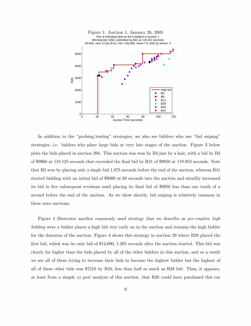
Figure 1: Auction 1, January 26, 2005

0 20 40 60 80 100 1200

1000

2000

3000

4000

5000

Auction Time (seconds)

Bid

s

Plot of individual bids by the 6 bidders in auction 1Winning bid, 5350, submitted by B41 at 119.421 seconds

45 bids, max 14 (by B11), min 1 (by B8), mean 7.5, bids by winner: 2

High bidB5B8B11B28B36B41

In addition to the “probing/testing” strategies, we also see bidders who use “bid sniping”

strategies, i.e. bidders who place large bids at very late stages of the auction. Figure 3 below

plots the bids placed in auction 394. This auction was won by B3 just by a hair, with a bid by B3

of $9960 at 118.125 seconds that exceeded the final bid by B41 of $9950 at 119.953 seconds. Note

that B3 won by placing only a single bid 1.875 seconds before the end of the auction, whereas B41

started bidding with an initial bid of $9000 at 68 seconds into the auction and steadily increased

its bid in five subsequent revisions until placing its final bid of $9950 less than one tenth of a

second before the end of the auction. As we show shortly, bid sniping is relatively common in

these auto auctions.

Figure 4 illustrates another commonly used strategy that we describe as pre-emptive high

bidding were a bidder places a high bid very early on in the auction and remains the high bidder

for the duration of the auction. Figure 4 shows this strategy in auction 29 where B28 placed the

first bid, which was its only bid of $14,690, 1.265 seconds after the auction started. This bid was

clearly far higher than the bids placed by all of the other bidders in this auction, and as a result

we see all of them trying to increase their bids to become the highest bidder but the highest of

all of these other bids was $7210 by B16, less than half as much as B28 bid. Thus, it appears,

at least from a simple ex post analysis of this auction, that B28 could have purchased this car

6

Figure 2: Auction 3, January 26, 2005

0 20 40 60 80 100 1200

1000

2000

3000

4000

5000

6000

7000


Bid

s



High bidB5B8B9B11B28B36B41

Figure 3: Auction 394

0 20 40 60 80 100 120

7500

8000

8500

9000

9500

10000


Bid

s



High bidB1B3B6B11B41B47B49

7


0 20 40 60 80 100 120

4000

5000

6000

7000

8000

9000

10000

11000

12000

13000

14000


Bid

s



High bidB5B8B11B16B28B36B38B41

much more cheaply by starting to bid low and gradually increasing its bid over the course of

the auction, instead of precommitting to a very high bid at the start of the auction. While it is

easy to make these judgements in hindsight, having access to data that no single bidder possesses

individually, it does appear hard to rationalize a strategy of making a high initial bid on purely a

priori grounds. Bidding a high amount early in these auctions comes with the risk of overpaying,

and bidding a low amount early in the auction entails a risk of being outbid later in the auction

and of revealing potentially valuable information to other bidders.

Auction 32, shown in figure 5 below, exhibits the non-monontic bidding behavior that we

observe by some bidders in some auctions. We see that the winning bidder in this auction, B11,

frequently reduced its bid including reducing its bid to very low values, $3000 and below, (lower

than any other bids, including its own bids, earlier in the auction), but then dramatically increased

its bid to win in the final milliseconds of the auction. It does not seem reasonable to attribute

the frequent reductions in bids to keyboard errors or “trembles” on the part of B11. Instead, the

bids seems to be intentional, and perhaps an effort to confuse other bidders. Most of the other

bidders placed monotonically increasing bids, though one other bidder, B8, also reduced its bid

to just below $4500 from a previous bid of $6000 before raising its bid again to about $6200 in

the final seconds of the auction.

8

Though the bidding behavior in this particular auction is not typical of the bidding in most of

the auctions in our data set, it does clearly illustrate the range of possible bidding strategies that

bidders might anticipate. B11’s non-monotonic bidding behavior does seem hard to rationalize

on strategic grounds. If bidders realize that they are obligated to pay the highest bid they submit

if this bid turns out to be the highest bid in the auction, what benefit do they expect to get from

reducing their bid later in the auction? Notice that reducing one’s bid precludes one from finding

out whether another bidder had outbid the previous high bid — at least temporarily until the

bidder raises the bid up again. Thus, we are at a loss from this casual initial analysis of the data

to see what benefit the bidder B11 expected to get from frequently decreasing its bid during this

auction. Perhaps B11 was reducing its bid to try to confuse its opponents? However by reducing

its bid, B11 was at least temporarily reducing the information it would be able acquire in the

auction since if it had not reduced its bid, it would have been able to see if its previous high bid

had been beaten by another bidder.

In auction 32, the winner was B11 though there was a subsequent bid by B38 just 47 millisec-

onds before the end of the auction equal to the $6390 placed by B11. The auction software uses

time priority as a tie breaker in case multiple bidders have the same highest bid, so this is why

B11 won. Notice that after submitting its winning bid of $6390 1.204 seconds before the end of

the auction, B11 submitted another bid of $2990 438 milliseconds before the end of the auction.

Could this reduction in its bid have affected the other high bidder, B38? This seems doubtful

since bidders are committed to paying the highest bid they submitted during the auction even

if they subsequently reduce their bids, and further no other bidders will observe a bidder who

reduces their bid (since the software only tells each bidder whether or not their highest bid is also

the highest bid in the auction so far). Thus, B11’s high bid of $6390 was still “on the table” even

though it reduced it to $2990 438 milliseconds before the end of the auction. If B38’s last bid

at 47 millesconds before the end of the auction had been slightly higher, it is doubtful that B11

would have realized it had been outbid in time to submit a slightly higher bid. Thus, we can see

no strategic advantage to adopting B11’s non-monotonic bidding strategy in this auction.

These auction results raise some immediate questions: if the auction rules allow bidders to

reduce their bids, could it ever be an equilibrium response for the bidders to use non-monotonic

bidding strategies — i.e. placing high bids early on in the auction to try to learn where the high

9


0 20 40 60 80 100 1202500

3000

3500

4000

4500

5000

5500

6000


Bid

s



High bidB5B6B8B11B16B17B28B36B38B41

bid might be, but lowering their bid later in the auction at B11 did in auction 32 shown above?

If the answer is no, then these examples suggest that some sort of model of boundedly rational

bidding behavior may be more appropriate for analyzing these auctions.

We also see that there is some randomness in when the auction actually ends. Though the

auctions are supposed to last 120 seconds, we see a number of auctions where the last bid is

time stamped at over 120 seconds, in some cases as late as 121 seconds. The auction software

accepts these late bids perhaps to allow for some communication delays. However it makes the

determination of the actual termination rule somewhat complicated. How do bidders know when

it will be too late to place a bid? This probabilistic nature of when some of these auctions end

complicates the use of bid sniping strategies since it is not a practical possibility to submit a

single bid in the very “last instant” of the auction. To our knowledge the rental company was

not intentionally using a soft close similar to the rules used by Amazon and eBay discussed in

Ockenfels and Roth [2014].

It is not immediately clear, given the limited information conveyed in the early stages of the

auction, what value bidders get from participating early in the auction as opposed to the strategy

of waiting to the last minute and placing a single clinching bid. If all bidders adopted the latter

strategy, this auction would start to resemble a one shot first price sealed bid auction, and the

10

auction outcomes could probably be well approximated using this standard and commonly used

auction model.

What we do not know at present is what effect the option to place early bids has on a bidder’s

subsequent bidding decisions. From a single bidder’s standpoint, it appears that having the option

to bid early could have value as it enables a bidder to safely “test the waters” by placing low bids

and gradually increase them, hoping that they can obtain a good deal. On the other hand, given

the coarse nature of information revealed over the auction (with each bidder being unable to see

competing bids) it is not immediately clear that bidders will do any better under this auction

format than in a standard one shot first price sealed bid auction.

However given the large number of auctions we observe and the large number of bids submit-

ted by each bidder in each auction, we think these data present both an interesting theoretical

and empirical challenge. We observe a variety of bidding behaviors in these auction, with a com-

bination of early bidders and late bidders, and in the extreme, the “snipers” who come in with

high bids in the very last instants of the auction. In particular, the number of bids submitted per

second increases dramatically in the final second of the auction as bidders jockey frenetically to

submit the winning bid.

2.1 Auction Statistics

We present a few statistics summarizing the auctions and bidding behavior in this section. In

particular, we quantify the frequency of different types of qualitative bidding strategies, including

“bid sniping” and “pre-emptive high bidding” where the latter indicates bidders who place the

winning bid very early in the auction. We are studying a population of experienced expert bidders,

since the 67 bidders participating in these auctions represent broker/dealers and they bid in an

average of 1281 auctions. The bidder with the most experience was B11 who bid in 7167 auctions,

though 20 of the 67 bidders were infrequent participants who bid in fewer than 100 auctions in our

sample of 11279 auctions. This total number is slighltly lower than the total number of auctions

we have, 11790, because we excluded 511 auctions where either the auction lasted significantly

longer than the 2 minute duration of the vast majority of auctions the rental company conducted,

or there were other problems that resulted in the car not actually being sold, as well as cases

where technical problems caused the winning price in the auction not to be the actual transaction

11

price that was ultimately paid by the winning bidder.

We observe substantial variation in the “win rate” (i.e. the fraction of auctions that a bidder

participates in and submits the winning bid), ranging from a low of 0% for bidder B45 to a high

of 39% for bidder B72. The average win rate among the 67 bidders is 13%. There is no obvious

correlation in the number of auctions bidders participate in and the win rate: some of the most

frequent bidders have below average win rates, such as B11 (the bidder that participated in the

largest number of auctions) or B49, who participated in 5385 auctions but has a win rate of

just 4.4%. The bidder with the highest win rate, 39%, participated in only 211 auctions. Of

course, having a high win rate is not necessarily evidence of a “successful” bidding strategy since

it is possible to increase the win rate by bidding more aggressively, but at the potential cost of

overpaying for the vehicles the bidder wins. Some differences in the win rate may also be due to

bidders who specialize in buying certain types of cars that may be in higher demand than other

types of less desirable vehicles.

Of the 11,279 vehicles sold in the auctions, the average selling price was $9621, though there

is substantial heterogeneity: the highest sale price was $100,000 and the smallest was $100. We

generally have the information on the make and model of the vehicles that were sold at auction,

however we do not have data on the odometer and age of sale for all 11,281 of these vehicles. We

know the age of the vehicle for a subsample of 8722 auctions, and the average age of these cars

was 1063 days (or about 2.9 years old), with the oldest vehicle auctioned was just over 6 years

old, and the youngest was only 56 days old (from date of acquisition as a new car). In some cases

relatively new cars are sold due to accidents, or due to other special circumstances. We have

information on the odometer value of the car in 7344 auctions, and the average value is 73,719.2

To better understand statistical regularities in the two minute bidding procees, figure 6 plots

2The rental company we study sells its rental cars at an average age and odometer value thatare significantly larger than the average age and odometer values that typical rental car companies inthe U.S. sell their vehicles, even though there is a recent trend toward holding vehicles longer evenby U.S. rental car companies. A Wall Street Journal article notes that “The average holding timefor a car at Hertz has grown to 18 months in 2012 from 10 months in 2006, for example.” (seehttp://online.wsj.com/news/articles/SB10001424127887324463604579040870991145200). In terms ofodometer values at replacement, an MSN blog by Clifford Atiyeh states that “By the time the averagerental-car retires, it’s a year old with between 35,000 to 40,000 miles on the clock, about 75 percent moremileage than in 2005. At that time, rental companies were replacing a greater number of cars that wereonly four to six months old with about 17,000 miles, according to Tom Webb, Manheim’s chief economist.’(http://editorial.autos.msn.com/blogs/autosblogpost.aspx?post=0851c06c-1d4f-4bf1-af57-d157cd777808).Cho and Rust [2010] analyzed the replacement decisions of the rental car company who provided our data andfound that this firm could increase its profits significantly (by up to 40%) by selling its rental vehicles at about150,000km and 5 years of age.

12

Figure 6: Rescaled Bid Trajectories

0 20 40 60 80 100 1200.55

0.6

0.65

0.7

0.75

0.8

0.85

0.9

0.95

1


Res

cale

d B

ids

Plot of rescaled bid trajectories

High bidMean Bid

0 20 40 60 80 100 1200.5

0.55

0.6

0.65

0.7

0.75

0.8

0.85

0.9

0.95

1


Res

cale

d B

ids

Plot of rescaled bid trajectories

Mean bid, auctions with bids in first 5 secondsMean bid, auctions with first bids after 5 secondsMean high bid, auctions with bids in first 5 secondsMean high bid, auctions with first bids after 5 seconds

the mean values of the rescaled bids in the auctions as a function of the elapsed time in the

auction. We rescaled the bids by dividing the bids by the winning (highest) bid in the auction,

and thus all of the rescaled bids are in the [0, 1] interval. Since this is an ascending price auction,

the bids naturally increase as a function of elapsed time in the auction. The left panel of figure 6

compares the mean high bid and the mean of all bids received as a function of elapsed time t. We

see the anomalous result that the expected bid trajectory actually tends to decrease during the

first five seconds of the auction before they turn around and start increasing during the remaining

115 seconds of the auction period.

This anomalous pattern reflects a compositional effect, a reflection of the prevalence of early

winning bids such as was illustrated in the case of auction 29 in figure 4. There are 1046 auctions

out of the universe of 11790 auctions where bids were submitted within the first second of the

start of the auction. In 255 (24%) of these auctions the winning bid was also submitted in the

first second of the auction, and in the remaining 791 auctions where bids were submitted in the

first second but the winning bid was made after the first second of the auction, the mean rescaled

high bid was 79%. This is still higher than the mean rescaled value of the first bid in a typical

auction, which is 64.5% and was submitted 14 seconds into the auction. So we conclude that

there appears to be some heterogeneity in bidding in these auctions: some bidders place relatively

high early bids very early into the auction for certain cars.

The right hand panel of figure 6 sheds further light on this. It compares the mean bid and mean

13

Figure 7: Cumulative probabilities of first bid and winning bid by elapsed time in auction

0 20 40 60 80 100 1200

0.1

0.2

0.3

0.4

0.5

0.6

0.7

0.8

0.9

1Probability that no bid and winning bid have been submitted, by elapsed time in auction


Pro

babi

lity

No bid submitted yetWinning bid submitted

high bid for bids received at different times during the auction for two different subsamples of

auctions: a) 8242 auctions where there were no bids in first 5 seconds, and b) 3548 auctions where

there were bids in first 5 seconds of the auction. We see that the average of all bids received are

essentially identical for these two subsamples after the first five seconds of the auction, whereas

the average of the high bids received in subsample b) is significantly higher. This leads us to

conclude that the difference in trajectories are due to a subset of “overly eager bidders” who

place very high bids right away in the auction for certain vehicles, perhaps for vehicles that they

have especially high valuations for, or which they may have overbid for. Additional evidence in

favor of this is that the mean sale price for the 1046 vehicles where bids were placed in the first

second of the start of the auction is $10610, over $1000 more than the average selling price in all

11790 auctions. If we further condition on the 255 auctions where the winning bid was submitted

in the first second of the auction, the mean selling price is almost $1000 higher, $11324. The

standard deviation of this mean sales price in these 255 auctions is $436, so the price difference

is statistically significant.

It is not clear that bidding a large amount for a vehicle in the opening instant of an auction

is an especially wise strategy. Recalling our discussion of the outcome of auction 29 in figure 4,

14

Figure 8: Distribution of submission time and order of the winning bid in the auction

0 20 40 60 80 100 1200

0.01

0.02

0.03

0.04

0.05

0.06

Distribution of time of winning bid

Den

sity

Time in auction (seconds)

Mean 107.0714Median 119.015Minimum 0.062Maximum 125.312Std dev 27.1972N 11277

0 0.2 0.4 0.6 0.8 10

0.1

0.2

0.3

0.4

0.5

0.6

0.7

0.8

0.9

1Distribution of percentile order of winning bid

Cum

ulat

ive

Pro

babi

lity

Percentile order of winning bid (1= winning bid is last bid)

Mean 0.86086Median 0.95122Minimum 0Maximum 1Std dev 0.24601N 11277

these high early bids could reflect a naive bidding startegy that cause these bidders to significantly

overpay relative to a more patient bidding strategy used by most of the bidders, which is to start

bidding at a low price and gradually raise the bid over the course of the auction in an attempt to

discover what the highiest bids of the other bidders will be. We found that 41 of the 67 bidders

placed these pre-emptive early bids in the first second of the auction. However of these, four

bidders — B28, B11, B47 and B10 — made such pre-emptive early bids in an average of 17

auctions each.

Figures 7 and 8 confirm that the dominant pattern is for the bidders to delay the submission

of bids and for the winning bid to be submitted quite late in the two minute auction. The red

curve in figure shows the cumalative probability that no bid has been submitted in the auction

as a function of time in the auction. Thus, a first bid has been submitted in virtually all of the

auctions by the 60 second point, the median time of submission of a first bid is about 10 seconds,

and the mean time at which a first bid is submitted is 14 seconds into the auction.

The blue curve plots the cumulative distribution of the time of submission of the winning bid.

This distribution is clearly skewed towards the end of the auction: the median time at which the

winning bid is submitted is at 119 seconds, just 1 second before the end of the auction and the

mean time is 107 seconds. The left hand panel of figure 8 also displays the probabilitiy density of

the time at which the winning bid is submitted and we do indeed see a small bump in this density

around 0 that reflects a small fraction of auctions where high pre-emptive submitted just after

15

Figure 9: Bids submitted per second in the auction

0 20 40 60 80 100 1200

0.5

1

1.5

2

2.5

3Average number of bids submitted per second


Ave

rage

num

ber

of b

ids

subm

itted

per

sec

ond

the auction starts. The right hand panel of figure 8 displays the order in which the winning bid is

received, i.e. it displays the cumulative distribution of the winning bid percentile ordering. That

is, if the winning bid is the first bid that was placed in the auction, its percentile ordering is 0 since

there are no bids that were placed before it. On the other hand if the winning bid was the last

bid submitted in the auction, its percentile is 1 since all of the bids in the auction where placed

before it. We find that the winning bid was the first bid in only 3.2% of the auctions, whereas it

as the last bid submitted in 27% of the auctions. The mean percentile is 86%, which means in a

typical auction 86% of the bids were submitted before the winning bid, and 14% of the bids will

are submitted after the winning bid was submitted. The median value is even higher: 95%, which

indicates that in 50% of the auctions only 5% of the bids in the auctions are submitted after the

winning bid.

Figure 9 provides additional evidence that the rate of bidding activity is the highest in the

final second of the auction. It shows the average number of bids submitted in one second intervals

in the auction at various times in the auction. On average one new bid arrives each second in

the auction, but in the final second (i.e. all bids arriving after 119 seconds into the auction) an

average of 2.8 bids are received. Since there is some randomness in the exact ending time of the

auctions (37% of the auctions received a last bid after 120 seconds, and the mean time of the

16

Figure 10: Cumulative distributions of recsaled bids by elapsed time in auction

0 0.2 0.4 0.6 0.8 10

0.1

0.2

0.3

0.4

0.5

0.6

0.7

0.8

0.9

1

High Bid as a Fraction of Winning Bid in the Auction

Cum

ulat

ive

Dis

trib

utio

n of

Hig

h B

id

CDFs of high bid (rescaled) by time bid was submitted

15101520406080100120

last bid for these auctions was 120.5 seconds), we would expect a somewhat higher value of the

mean bids per second given that our definition of the “last second” of the auction is an interval

that actually lasts an average of 1.2 seconds when we account for late bids that are allowed by

the auction software. However the value of 2.8 bids in the last second cannot be accounted by

the fact that the “last second” actually last 1.2 seconds when we account for late arriving bids.

The increased bidding frequency in the last second is also accompanied by an acceleration in the

bidding increments, as reflected by the convex shape of the the mean value high bid in the final

second of the auction as shown in left hand panel of figure 6.

The overall conclusion that we draw from this is that a) winning bids are submitted very

late in the auction, and b) as a consequence, they do not remain on the the table for very long:

the mean duration of the winning bid is 11.8 seconds, but the median duration is 0.875 seconds,

reflecting the fact that the fact that in 50% of the auctions the winning bid was submitted after

119 seconds into the auction, with less than a second of remaining time before the auction ends.

There is a notable acceleration in both the rate of submission of bids and in the rate of increase

in both the high bid and the average bid in the closing second of the auction.

Figure 10 plots the cumulative distributions of the rescaled high bids as a function of the time

in the auction. Consistent with the ascending bid nature of the auction, we see a natural pattern

17

of stochastic dominance in these distributions. That is, if Ft(b) is the CDF of the high bid received

by second t into the auction, we have Fs ≻ Ft in the sense of first order stochastic dominance if

s > t. So we see that in the first second of the auction, the CDF F1(b) indicates that the high

bid is 0 in over 90% of the auctions — that is, no bid has been submitted by the end of the first

second in over 90% of all auctions. The fraction of auctions where no bid has been submitted

steadily falls as t increases, so that by 10 seconds into the auction the blue dotted line in figure 10

indicates that a positive high bid is on the table in more than 50% of the auctions in our data set,

and the median value of the high bid is about 50% of the eventual winning bid submitted in the

auction. The distribution of bids collapses about a unit mass as a rescaled bid of 1 (i.e. the high

bid in the auction) as t → 120. However the convergence to a unit mass is not perfect, and we see

that F120(1) < 1 due to the fact that the auction software allows for short delays in submission

of final bids and final bids were received shortly after 120 seconds in over 36% of all auctions in

our data set. Thus, there is some residual uncertainty that a high bid could be bettered even for

high bids that are submitted slightly after 120 seconds into the auction.

Figure 11 shows the distribution of the number of bidders participating in an auction and

the total number of bids submitted per auction (by all bidders). We see that there is are an

average of 7.6 bidders participating in an auction and an average of 59 bids are submitted, so

each bidder submits on average 7.8 bids per auction. Interestingly, there were 22 auctions where

only a single bidder was bidding in the auction. Of course, reasonable prices are possible in this

situation because of the fact that bidders are not aware of the number of other bidders who are

participating in any auction: they only see whether their current bid is the highest or not. While

a bidder who is the only bidder in the auction will see that they have the highest bid in every

instant (after they have submitted their bid), the bidder may conclude that they have overbid, or

that there are other bidders who have not yet submitted a bid and, as a result, the bidder may

actually be tricked into increasing their bid in the auction even though they are actually facing

no competition at all! Indeed, the average number of bids submitted in the 22 auctions where

only a single bidder had entered the auction was 7.7, virtually the same as the average number

of bids per bidder in auctions when there are multiple bidders participating in the auction.

The fact that we found that most winning bids are placed very close to the end of the auction

and that a high proportion of winning bids are actually the last bid submitted in the auction

18

Figure 11: Distribution of number of bidders and bids submitted in an auction

0 5 10 15 200

0.05

0.1

0.15

Distribution of number of bidders

Den

sity

Number of bidders in the auction

Mean 7.6069Median 7Minimum 1Maximum 20Std dev 2.718N 11279

0 50 100 150 2000

0.002

0.004

0.006

0.008

0.01

0.012

Distribution of number of bids submitted

Den

sity

Number of bids submitted per auction

Mean 59.0703Median 54Minimum 1Maximum 227Std dev 32.0181N 11279

leads to the question as to whether bid sniping is a frequently used bidding strategy in these

auctions. We define an auction as being won by a bid sniper if the winning bidder submits a

single bid in the final two seconds of the auction. Using this definition, we find that 520 of the

11279 auctions we analyzed (4.6%) were won by bid snipers. A total 37 of the 67 bidders in

these auctions used bid sniping strategies, though it was far from the exclusive strategy/behavior

that they exhibited. The most frequent bid snipers were B58 (who sniped in 134 of the 1520

auctions they bid in, or 8.8% of the time), follows by B65 who sniped in 3.9% of the auctions they

participated in, B23 who sniped 2.6% of the time and B1 who sniped 2.3% of the time. However

these are the frequencies of successful sniping, i.e. where the bidder was able to win. We should

put the adjective “successful” in quotation marks since it is not evident a priori that sniping is

an effective bidding strategy. Similar to high pre-emptive early bidding, snipers are not engaging

in the opportunity to learn the current high bid earlier in the auction and thus could be winning

by significantly overpaying for the cars they bought.

We can consider a weaker notion of bid sniping by defining a sniper to be any bidder who

submits a single bid in the last two seconds of the auction, regardless of whether they win the

auction. A bid sniper was present in 2502 of the 11279 auctions (or 22% of all auctions). In most

of these auctions only a single sniper was present, but there were multiple snipers in 293 auctions.

A total of 54 of the 67 bidders in our data set engaged in bid sniping in some auction, though

their proclivity to snipe varied significantly, from less than 1% to a high of 26% by the bidder who

19

sniped most frequently, B28. The win rate for bid snipers is about the same as the overall win

rate: about 13%, however a number of bidders who frequently snipe have a significantly higher

win rate from the auctions where they sniped compared to ones where they did not snipe. For

example B58 has a win rate of 34% on the auctions where it sniped, which is higher than its

overall win rate of 29%. B1, who sniped in 9% of the auctions it participated in, had a 26% win

rate for these auctions compared to an overall win rate of 14%. For the auctions where a bidder

sniped but lost the auction, their (losing) bid was on average 83% of the winning bid. The bidders

who sniped more frequently and had higher win rates in the auctions they bid in also bid a higher

fraction of the winning bid in the auctions they lost. For example, the most frequent sniper, B58,

submitted bids that were an average of 90% of the winning bid in the auctions where B58 sniped

but lost the auction. B1, another frequent sniper whose win rate in auctions where it sniped is

significantly higher than its overall win rate, bid 93% of the winning bid in the auctions where it

sniped but lost.

Besides pre-emptive early bidding and bid sniping, we observe a fair amount of what we might

describe as irrational or uninformative bidding in the auctions. This occurs whenever a bidder

submits a bid that is at the same value or lower than an previous bid that the bidder had already

submitted. Given the rules of the auction where only the highest submitted bid is recorded,

there appears to be no rationale for submitting these types of bids, and they can’t even have a

signalling value to other bidders since the auction software (by virtue of only showing whether

or not a bidder’s current bid is the current highest bid in the auction) prevents other bidders

from being aware that a bidder has lowered their lower bid. In some cases we might expect a

submission of a bid that is lower than a previously submitted bid would be simply a mistake, a

typing error on the keyboard for example. However for most bidders who do this, it happens too

frequently to chalk this up to a mistake. For example the bids placed by B11 in auction 32 in

figure 5 show a systematic zig-zag pattern that can only be ascribed to an intentional pattern of

bidding. However it is not clear what the objective of this is, other than perhaps being a sign

of boredom or capriciousness by the person placing the bids. Out of 85798 bidding histories we

analyzed (the total number of bid histories by all bidders who participated in the 11279 auctions

in our data set), we observed bidders repeating the same bid at one or more instances in the

auction in 12502 cases (14.6% of the histories) and one or more decreases in their bid in 6556

20

cases (7.6% of the histories).

Overall, while we do observe both pre-emptive early bidding and sniping behavior and a high

incidence of uninformative bidding in these auctions, by far the most commonly used bidding

behavior that we observe is bid creeping where a bidder makes a succession of increasing bids

closely spaced in time in an attempt to find out what the current high bid is. Examples of bid

creeping are the bids by B5, B11, B28 and B36 in auction 1 in figure 1, the bids by B5, B11,

B36 and B41 in auction 26, or bids by B5, B11, B36 and B41 in auction 26 in figure 2 or bids

by B1, B6, B41 and B47 in auction 394 in figure 3. Bid creeping seems to be reasonable strategy

for learning what the current high bid in the auction is, since it avoids the risk of overbidding

that might be implied by a bid jumping strategy which is similar to bid creeping but involves

bid sequences that are spaced further apart and jump up in higher increments compared to bid

creeping. Examples of bid jumping strategies include the sequences of bids by B41 in auction 1

in figure 1, and B1 in auction 394 in figure 3. Of course the dividing line between bid creeping

and bid jumping is a fuzzy one: the two behaviors are both consistent with a desire to learn what

the current high bid in the auction is, but in bid creeping the bidder is willing to make a much

larger number of bids in rapid succession, each one only slightly higher than the previous one,

whereas in bid jumping the bidder seems to have a higher psychic cost of placing bids and tends

to make fewer bids at more widely spaced intervals of time in the auction, and the increments

over the previous bids are larger. Thus, bid jumpers seem to behave as if they had a higher cost

of submitting bids and/or are more willing to take the risk of overbidding to become the current

higher bidder relative to what we observe for bid creepers.

In summary, we have identified a number of different bidding behaviors in these auctions:

1) pre-emptive early bidding, 2) bid sniping, 3) bid repeating and decreasing behaviors, 4) bid

jumping, and 5) bid creeping. We analyzed the 11279 auctions in our database with regard to

the type of strategies employed by the winning bidder and we found that bid creeping was the

predominant strategy employed by the winning bidders, in 52% of all auctions. We found that bid

jumping and behaviors that involve a mix of creeping and sniping were the next most common

behavior, used by the winning bidder in 20% of the auctions. We observed bid sniping in nearly

5% of all auctions (where the winner submitted a single bid in the remaining 2 seconds of the

auction), and pre-emptive early bidding in nearly 3% of all auctions (where the winner submitted

21

a single bid but in the first 2 seconds of the auction).

When we analyzed the types of bidding behaviors on a bidder-by-bidder basis, we find a

distribution of behaviors for each of the bidders — i.e. no bidder always bids exclusively using

one type of “strategy” (e.g. bid sniping) in all of the auctions they participate in. We tabulated

the distribution of various types of bidding behaviors for the 67 bidders in the auction and the

most common behavior for virtually all of the bidders is bid creeping, and the next most common

behavior was bid jumping (or a mix of creeping and jumping behaviors).

In the next section we analyze this auction from a theoretical perspective to see what we

can say about the properties of rational, equilibrium bidding strategies, and whether the actual

bidding behavior we observe in these auctions at all resembles the equilibrium bidding behavior

predicted by theory.

3 Can game-theoretic models explain early bidding?

In this section we consider dynamic, equilibrium models of bidding in the rental car auctions,

and whether the behavior we observe could be consistent with a Perfect Bayesian Equilibrium

(PBE) of the auction, formulated as a dynamic game of incomplete information. Due to the severe

restrictions on information provided to bidders in these auctions, the amount they can learn about

each other over the course of the auction is quite limited. Therefore it is far from clear that the

option to bid early in the auction has significant value. In fact, in discrete time approximations to

the continuous time bidding game there always exists an uninformative equilibrium in which no

bidders submit bids until the final second of the auction, at which point they submit bids equal

to the values they would submit in a static sealed bid auction. For example Ockenfels and Roth

[2006] proved this, even under a “soft close” where the ending time of the auction is probabilistic

(such as sometimes occurs in this auction as we saw in the previous section).

However the empirical evidence provided in the last section is manifestly inconsistent with the

hypothesis that the behavior in these auctions are realizations of the uninformative equilibrium to

the dynamic auction game. Even though there tends to be a rush of bids placed in the final second

of the auction, there is a high level of bidding activity throughout the two minute auction, and

many winning bids are submitted well before the final second of the auction, as we demonstrated

22

in section 2.

It is possible that there may be PBE of the dynamic auction that involve early bidding, but

these bids are not “serious bids”, so that the resulting PBE is strategically equivalent to the

uninformative equilibrium. That is, there may be PBE in which early bidding is regarded as

uninformative “cheap talk” that is ignored by the bidders when they submit their “serious” bids

in the final second of the auction. We are not interested in such equilibria, however. Instead

we are interested in whether there exist PBE where bidders do place serious bids early in the

auction and they are able to gather significant information from their bidding activity during

the course of the auction. We believe the analysis of the previous section suggests bidders are

indeed bidding “seriously” early on in the auction and are attempting to learn what the current

high bid is by engaging in bid creeping and bid jumping. We will show in the following section

that knowledge of the current high bid in the auction significantly increases a bidders’ ability to

predict the final winning bid in the auction. This information should have value to bidders who

have high valuations for the item being auctioned by helping them to win without overpaying.

This implies that there could be a significant reward to bidders for undertaking “costly learning”

in the form of placing serious bids in the auction well before the last second of the auction, and

thus the possibility that there exist informative PBE with “serious” early bidding by bidders.

There are two main costs that bidders must incur to gather information and learn about

relevant unknown quantities in this auction: a) the psychic “effort” cost of paying attention

to the screen and typing in a bid (and making sure the amount is typed correct), and b) the

“commitment cost” that once a bid is submitted, the bidder is obligated to pay the amount of the

bid should it emerge as the high bid at the end of the auction. Thus, in attempting to learn what

the high bid is, a bidder must submit a bid that is higher than the current (unknown) high bid in

the auction, but there is a risk that in doing this the bidder will bid more than necessary. Bidders

can avoid such overbidding by bid creeping, but there is a trade off between the cumulative hassle

costs of submitting many bids that increase in tiny increments compared to using bid jumping

strategies that economize on the hassle costs of bidding but involve a risk of bidding more than

necessary to learn the current high bid in the auction.

If the costs to submitting bids and monitoring progress in the auction were zero, we would

expect all bidders would place large number of creeping bids during the auction. Intuitively there

23

should be a PBE that results in outcomes similar to that of an English auction where the current

high bid would steadily rise over the course of the auction to the valuation of the second highest

bidder, and the auction would be won by the bidder with the highest valuation but with a winning

bid equal be the smallest bid increment (e.g. 1 cent or 1 dollar) above the value of bidder with the

second highest valuation. However if psychic costs of placing very frequent bids and monitoring

the auction on a millisecond by millescond basis are too high for most bidders, then we would

expect more bidders to use jump bidding strategies that involve placing bids less frequently and

with higher increments in each successive bid than in the case of the bid creeping strategies we

would expect to see if these costs were zero.

To our knowledge there are no fully analyzed equilibrium models of bidding in this type of

auction environment. The closest related work that we are aware of is Groeger and Miller [2013]

who analyze an informationally similar auction environment where the items being auctioned are

CDs (certificates of deposit) and the bidders are banks. These auctions are also conducted online,

and similar to the auctions we study, the bidders are not aware of the number of competing

bidders participating in the auction, nor are they aware of the current high bid in the auction

except when the bidder’s bid is the highest current bid in the auction. Groeger and Miller [2013]

analyze some of the properties of a PBE of this auction game, though they do not fully solve the

game or characterize the set of PBE or the more detailed properties of any particular PBE.

In addition, they abstract from some of the informational constraints that the actual bidders

face, such as assuming that bidders can observe the current high bid in the auction at any given

time even if they do not hold the current high bid (the current high bid in their terminology

is referred to as the “on the money” ONM bid and a bid that is below the high bid is “out of

the money” OUTUM): “our model assumes that the bank observes the ONM rate whenever its

previous bid is OUTM.” (p. 12).

We believe this assumption sidesteps some of the challenging “costly learning” problems that

bidders face in these types of auctions and which is the focus of our analysis. Instead of modeling

the timing between the submission of bids endogenously, Groeger and Miller [2013] assume that

bidding is costless, but the times at which bidders are able to attend to the auction and submit new

bids is exogenously determined — a realization of a Poisson process: “Because the institutional

mechanism for updating a bid involves typing a few keystrokes on a computer, and banks creep

24

up to the ONM rate not seeming to economize on the number of bidding entries, our model also

assumes the act of bidding is not costly. Instead of continuously updating an ONM bid near

the end of the auction period, or sniping, more than half the winning banks submit their final

bids long before the auction ends: to accommodate these features of the data, the bidders in our

model have only imperfect monitoring capabilities. Intuitively there are competing uses for bank

time; alternatives to devoting attention to the auction and reacting immediately to changes in the

bidding history of that security, or being available to bid at the endpoint of the auction, include

monitoring other securities the bank trades in, seeking new clients, or engaging in administrative

work. In the model monitoring opportunities are modeled as random events, driven by a stochastic

process that is controlled by the bank at a cost.”

It seems reasonable to assume that there are competing tasks that may distract bidders during

these auctions, but it may not be easy to empirically distinguish between the Groeger and Miller

[2013] model where jump bidding arises from bidders who can bid costlessly but are exogenously

distracted from paying attention and being able to bid in the auction for random (exponentially

distributed) periods of time, with a model where bidders monitor the auction continuously (or

at least at a finite number of discrete points in time in our discrete-time approximation to this

game) but face both strategic and psychic costs of submitting bids. Our goal is to try to provide

an explanation of the timing and magnitude of successive bids as an endogenous outcome and

see if it is possible to explain the heterogeneous bidding behaviors such as bid creeping and jump

bidding as equilibrium outcomes in a model where bidders have endogenously asymmetric beliefs

and heterogenous psychic costs of submitting bids.

However even in the presence of some reasonable simplifying assumptions Groeger and Miller

[2013] must confront a host of difficult problems to provide an equilibrium analysis of the bidding

behavior in their auction. For example, since bidders do not know the number of competing

bidders or their valuations, they face an extremely difficult Bayesian learning problem to update

their prior beliefs about these important quantities based on signals received over the course of

the auction. However Groeger and Miller [2013] also sidestep the mechanics of this Bayesian up-

dating problem or the calculation of the perfect Bayesian equilibrium strategies implied by their

model. Instead their empirical analysis is based on a clever approach to the identification of the

underlying stuctural objects of their model that does not require them to solve for equilibrium

25

bidding strategies. We sympathsize with their choices because we conclude it is far too difficult

computationally to try to even numerically solve for the equilibria of this bidding game: the di-

mensionality of the “belief space” (which constitutes the state space of the dynamic programming

problems that bidders must solve to calculate their equilibrium bidding strategies) is far too large

to make it feasible to solve the game numerically.

Inview of these problems, we follow a strategy similar in spirit to Krusell and Anthony A. Smith

[1998] and Weintraub et al. [2008] and search for simpler non-Bayesian methods of learning and

belief-updating with parametric models that have “sufficient statistic” representations that result

in more tractable, lower dimensional dynamic programming problems for the bidders. We solve

for an “approximate equilibrium” where bidders employ effective methods of inference and learn-

ing, and their beliefs are approximately correct. We will describe these beliefs in more detail in

the next section. Unlike Groeger and Miller [2013], the goal of our analysis is not just to estimate

the underlying structural objects (e.g. the distribution of bidders’ valuations of different cars up

for auction, or their psychic costs of submitting bids). We also believe it is important to try to

actually solve for and provide a detailed characterization of the type of bidding behavior that

our theory predicts. While it would be desirable to calculate a Perfect Bayesian Equilibrium of

the dynamic auction, in addition to the daunting computational challenges described above, an

additional problem is the fact that these models are likely to have a vast multiplicity of equilibria.

It is not clear how bidders would coordinate on any particular one of these equilibria. So far

we have only been able to take some first baby steps in numerically computing a two bidder,

two period example in order to get some intuition. We describe the solution of this special case

example further below.

Daniel and Hirshleifer [1998] provide important insights in the nature of bidding in dynamic

auctions where bidders face costs of submitting bids. They consider a discrete time, alternating

move bidding game played between two bidders who have independently drawn valuations for an

item up for auction. One bidder moves first and declares a bid for the item which is observed

by the opponent. The other bidder can either pass (in which case the first bidder wins the item

and pays the amount it bid), or submit a higher competing bid. The bids can continue increasing

in this alternating fashion until one of the bidders passes and the auction ends and the winning

bidder pays the amount it bid. Daniel and Hirshleifer [1998] prove that when there are costs of

26

submitting bids that “bidding occurs in repeated jumps, a pattern that is consistent with certain

types of natural auctions such as takeover contests”.

Besides improving our understanding of a new auction institution, a separate practical moti-

vation for conducting a structural study that hypothesizes that bidding is in equilibrium, or at

least in some sort of “approximate equilibrium” is to use the model to make counterfactual pre-

dictions of how changes in the auction mechanism would affect expected revenues to the seller, in

the spirit of Myerson [1981]. In particular, we are interested in what the potential gains might be

to conducting dynamic auctions compared to simpler static auctions such as the first price sealed

bid auction or the second price auction. When bidders’ valuations are indpendently distributed,

the Revenue Equivalence Theorem predicts that the expected revenue from selling the item in an

English auction, a first price sealed bid auction, or a second price auction will be the same. It

is tempting to appeal to the Revenue equivalence theorem to conclude the the expected revenues

from selling the item in a dynamic auction like the one we analyze will also be the same as in an

dynamic English auction or a static first price sealed bid auction.

However we think this conclusion is premature since the version of the Revenue equivalence

theorem proved by Myerson [1981] makes the important caveat that revenues are the same for

all mechanisms that have the same probability distribution for allocating the item. In standard

auction theory there is a focus on symmetric equilibria of the first price sealed bid auction, which

implies that with probability 1 auction outcomes are ex post efficient — i.e. the bidder with the

highest valuation wins the item. The English auction and the second price auction are also ex

post efficient, so Myerson’s version of the Revenue Equivalence Theorem predicts that all three

of these auction institutions should result in the same expected revenue to the seller.

However there are good reasons to believe that an informative PBE to the dynamic auction

we study is not ex post efficient. We conjecture this will be true even in a symmetric PBE of

the dynamic auction. The reason is that even when the strategies are symmetric, the restrictions

on the information made available to the bidders in the auction imply that bidders will have

differential information as the auction unfolds, and this results in endogenous asymmetries in their

realized bidding behavior. In particular, in an informative symmetric PBE, the first bidder to be

awarded the high bid in the auction will have different information than the other bidders. This

difference in information can cause the bidders to alter their subsequent bidding behavior even

27

though they are all using a common (symmetric) PBE bidding strategy. Further, we conjecture

that these endogenous asymmetries can result in ex post inefficient auction outcomes — i.e. the

bidder with the highest valuation for the item may not always win the auction. If this is true, then

the seller may earn either higher or lower expected revenue in the dynamic auction compared to

the revenue implied by a symmetric equilibrium to a first price sealed bid auction or the equilibria

any of the other auction mechanisms that result in ex post efficient outcomes.

We will provide a concrete example of ex post inefficiency in the PBE of the two period,

two bidder model below. However the intuition for ex post inefficiency in the general case is as

follows. Assume that there is a symmetric, informative PBE where bidders submit bids in every

period with probability 1. The after the first round of bids, the bidder who submitted the highest

bid can infer that they have the highest valuation for the item whereas the other bidders can

conclude that they do not have the highest valuations for the item but they are still unaware of

how many other bidders there may be in the auction, or what their valuations are. We cannot

necessarily conclude that the game is all over at this point and there is no point for the bidders

who realize they did not have the highest valuation to drop out. Instead this PBE may entail

more aggressive subsequent bidding by the bidders who “lost” the first bidding round and less

aggressive subsequent bidding by the winner of the first round (i.e. the bidder who submitted

the highest bid in the first round). Under this scenario, the difference in information results in

different bids, and this difference in bidding behavior in subsequent stages in the auction can

result in ex post inefficient outcomes.

Thus, one goal of the more “behavioral” aaproximate equilibrium approach to the analysis of

this auction that we conduct in section 4 is to be sure that the model can be used to generate

predictions of how bidders would react to alternative auction mechanisms such as a one shot

first price sealed bid auction and to compare the expected revenues that the rental company

could earn if it switched to an alternative auction format. Our conjecture is that due to the

combination of the psychic bidding costs, the endogenous asymmetries in information and the

implied ex post inefficiencies in auction outcomes, the rental company would earn higher expected

revenue if it switched to an English auction or a first price sealed bid auction. In fact, Cho et al.

[forthcoming, 2014] have already provided empirical evidence that this is the case. However

an English auction can generate higher expected revenues than the informationally-constrained

28

dynamic auction we study here, or a static first price sealed bid auction if there is affiliation

in the valuations of the bidders: this is an implication of the so-called linkage principle (see

Milgrom and Weber [1982]). In this analysis we assume that bidders’ valuations are independently

distributed, and in that case the Revenue equivalence principle implies that expected revenues

from an English and first price sealed bid auction would be the same. We conjecture that if there

is a failure of Revenue Equivalence with respect to the information-constrained dynamic auction

we study, the finding may be due the psychic bidding costs and ex post inefficiencies, and not

necessarily evidence that bidders’ valuations are affiliated.3

Rather than directly analyzing this auction as a continuous time game of incomplete informa-

tion, we will analyze it as a sequence of discrete time games of incomplete information where we

assume that the bidders can place bids at T equally spaced instants during the 2 minute auction,

so that the length of each time interval is ∇T = 120/T . We do not believe that this time dis-

cretization involves significant loss of generality, since the set of bidding opportunities in a finely

discretized discrete-time formulation of the game should not be materially constrained relative

to the actual continuous time version of the game. The only issue of potential concern is the

occasional probabilistic termination rule caused by the fact that the auction software sometimes

accepted bids that arrived a few milliseconds or tenths of a second after the end of the 120 second

auction. However the randomness in the termination can be approximated in discrete time by

a probabilistic horizon T . We will investigate the effect of a probabilistic auction termination

rule in the next section but at this point we do not think our results will be materially affected

regardless of whether T is a known constant or whether it is probabilistic, T provide the level of

variance in T is sufficiently small (and in section 2 we did find that the variance in T was indeed

small).

The analysis of discrete time equilibria is already challenging enough, though the coarse nature

of the information provided to the bidders reduces some of the complexities in the Bayesian

updating that bidders can do, and we use this to significantly reduce the dimensionality of the

3Saini [2012] finds evidence that endogenous asymmetries can be costly, but he studied a different aspect ofauction dynamics, repeated (static, sealed bid) procurement auctions. However there may be some strategic sim-ilarities in the dynamic considerations in analyses of bidding for multiple items in a sequence of static auctionsand bidding for a single item in a single dynamic auction. For example Saini [2012] concludes that endogenousasymmetries that can arise in a sequence of static auctions can also be costly for the procurer: “We find that theprocurer is best off scheduling frequent auctions for small project sizes. Otherwise, firm capacity utilization ratesbecome larger and more asymmetric, which softens competition and increases procurement costs.” (p. 726).

29

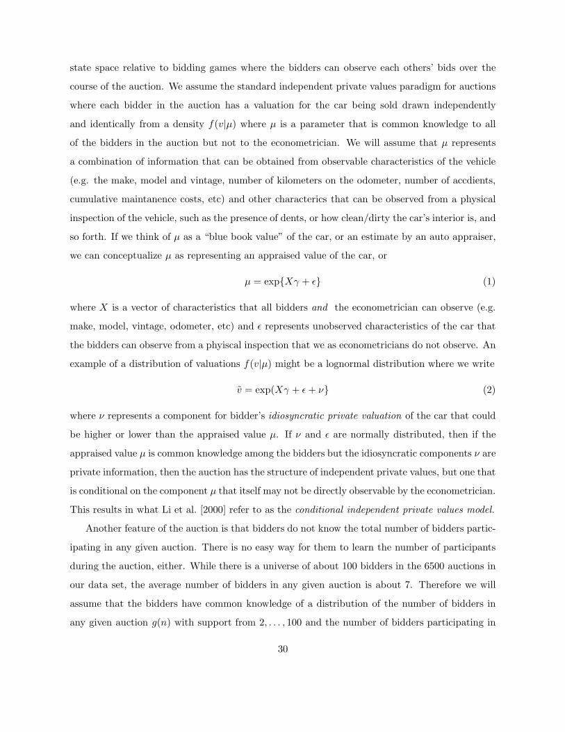
state space relative to bidding games where the bidders can observe each others’ bids over the

course of the auction. We assume the standard independent private values paradigm for auctions

where each bidder in the auction has a valuation for the car being sold drawn independently

and identically from a density f(v|µ) where µ is a parameter that is common knowledge to all

of the bidders in the auction but not to the econometrician. We will assume that µ represents

a combination of information that can be obtained from observable characteristics of the vehicle

(e.g. the make, model and vintage, number of kilometers on the odometer, number of accdients,

cumulative maintanence costs, etc) and other characterics that can be observed from a physical

inspection of the vehicle, such as the presence of dents, or how clean/dirty the car’s interior is, and

so forth. If we think of µ as a “blue book value” of the car, or an estimate by an auto appraiser,

we can conceptualize µ as representing an appraised value of the car, or

µ = exp{Xγ + ǫ} (1)

where X is a vector of characteristics that all bidders and the econometrician can observe (e.g.

make, model, vintage, odometer, etc) and ǫ represents unobserved characteristics of the car that

the bidders can observe from a phyiscal inspection that we as econometricians do not observe. An

example of a distribution of valuations f(v|µ) might be a lognormal distribution where we write

v = exp(Xγ + ǫ+ ν} (2)

where ν represents a component for bidder’s idiosyncratic private valuation of the car that could

be higher or lower than the appraised value µ. If ν and ǫ are normally distributed, then if the

appraised value µ is common knowledge among the bidders but the idiosyncratic components ν are

private information, then the auction has the structure of independent private values, but one that

is conditional on the component µ that itself may not be directly observable by the econometrician.

This results in what Li et al. [2000] refer to as the conditional independent private values model.

Another feature of the auction is that bidders do not know the total number of bidders partic-

ipating in any given auction. There is no easy way for them to learn the number of participants

during the auction, either. While there is a universe of about 100 bidders in the 6500 auctions in

our data set, the average number of bidders in any given auction is about 7. Therefore we will

assume that the bidders have common knowledge of a distribution of the number of bidders in

any given auction g(n) with support from 2, . . . , 100 and the number of bidders participating in

30

any given auction nt is an IID draw from the density g. Given nt the valuations of the bidders

(v1, . . . , vnt) are IID draws from f(v|µ). Given these bidders and valuations, the bidding on the

car starts at t = 1 and continues until t = T where T ≥ 2.

To start with the simplest possible case, consider the case T = 2 and under the belief that there

are only two possible bidders in the auction, i.e. g(2) = 1. We consider a symmetric equilibrium

where the two bidders use the same bidding strategy b1(v) to place bids given their valuation v in

time period t = 1 of the auction, and then in the next and final stage of the auction, t = 2 they

place updated bids from two bid functions {b2,l(v, b), b2,h(v, b)}. In game theoretic terms, we model

bidding as a two-player, two stage simultaneous move game of incomplete information, unlike the

alternating move formulation adopted by Daniel and Hirshleifer [1998]. We are interested in the

question of determining whether an informative symmetric equilibrium to this game exists. That

is, is there a PBE where both bidders use the same bidding strategies b1(v) and {b2,l(v), b2,h(v)}

that is also informative (i.e. where b1(v) is strictly monotonically increasing and b1(v) > 0 when

v > 0)?

The stage 2 bid functions depend both on the bidders’ values and on the bids that they placed

in stage t = 1, and also on the information they learned at stage 1, which can only be whether

their bid is the high bid or not. Thus, b2,h(v, b) is the bid placed by a bidder who has a value v

for the car and placed a bid of b at stage t = 1 and who had the high bid in stage t = 1. Similarly,

b2,l(v, b) is the bid placed by a bidder who has a value v for the car and placed a bid of b at stage

t = 1 and who had did not have the high bid in stage t = 1. Thus, the high bidder only knows

their own bid and the information that they have the high valuation and the low bidder in stage

t = 1 only knows their own bid and the information that they do not have the high valuation.

Here we are assuming that the initial bid function b1(v) is strictly montonic so that if bidder 1

has value v1 and bidder 2 has value v2 and v1 > v2, then b1(v1) > b1(v2) implies that v1 > v2.

But since bidder 1 is not informed of the bid submitted by bidder 2, bidder 1 only knows that

v2 is a random variable drawn from the conditional distribution of f(v|µ) given the additional

conditioning information that v2 ≤ v1 and this conditional distribution (CDF) is given by

F (v|µ, v ≤ v1) =F (v|µ)

F (v1|µ), v ≤ v1, 0 otherwise (3)

Similarly the low bidder at stage t = 1 only learns that he/she has a lower valuation than the

other bidder, but do not have any more specific info on the bidder of the high bidder, it follows

31

that the low bidder has a conditional distribution of valuations over its opponent given by

F (v|µ, v ≥ v2) =F (v|µ)− F (v2|µ)

1− F (v2|µ)v ≥ v2, 0 otherwise (4)

Now consider the equations determining the equilibrium bidding strategies, where we assume a

symmetric Bayesian Nash equilibrium of the two period game. The strategies are symmetric in the

sense that we are using a single set of bidding strategies (b1(v), b2,l(v, b), b2,h(v, b)) to determine

the bidders’ bids, even though this symmetric equilibrium does reflect the endogenous information

asymmetry that arises in stage t = 2 when the bidders submit their stage t = 2 bids. Of course,

this asymmetry comes from the information the bidders receive about whether they submitted

the high bid in stage t = 1. Thus, even though this is an incomplete information game, the players

start off using the same bidding strategy b1(v) to determine their initial t = 1 bids, because there

has been no information released at this stage to cause them to bid differently, other than the

difference in their valuations v1 and v2. But then at stage t = 2 with the stage 1 bids revealed the

bidders learn who has the high and low bids and this information causes them to use potentially

different bidding strategies at t = 1 given by b2,l(v, b) and b2,h(v, b), respectively.

We solve the bidding game by backward induction starting at stage t = 2. The bidding

strategies b2,l and b2,h must be mutual best responses, so they must satisfy the following equations

b2,h(v, b) = argmaxb′≥b

(v − b′)

∫ v

0

I{b2,l(v′, b1(v

′)) ≤ b′}f(v′|µ)dv′/F (v|µ)

b2,l(v, b) = argmaxb′≥b

(v − b′)

∫ ∞

vI{b2,h(v

′, b1(v′)) ≤ b′}f(v′|µ)dv′/[1− F (v|µ)]

where

b1(v) = argmaxb

(v − b2,h(v, b))

[∫ v

0

I{b2,l(v′, b1(v

′)) ≤ b2,h(v, b)}f(v′|µ)dv′

]

+

(v − b2,l(v, b))

[∫ ∞

vI{b2,h(v

′, b1(v′)) ≤ b2,l(v, b)}f(v

′|µ)dv′]

.

This is a system of functional equations and the stage t = 1 bidding function b1(v) affects the

stage t = 2 bid functions (b2,l, b2,h), and conversely these stage t = 2 bid functions affect the stage

t = 1 bid function b1 (and note also from equation (5) that b1 must also be a best response to

itself). Notice that the amount the winner pays in stage t = 2 of the auction is max(b′, b), where

b′ is the amount bid in stage t = 2 and b is the amount bid in stage t = 1. This is a consequence

of the auction rules already discussed and is reflected in equation (5). Thus, even if either bidder

32

lowered their bid in stage t = 2, they would still be obligated to pay the amount they bid in stage

t = 1, b, if this turned out to be the high bid in the auction.

We now show that the informative PBE exhibits endogenous asymmetry — i.e. b2,h(v, b1(v)) 6=

b2,l(v, b1(v)). The equilibrium solution in stage 2 results in more agressive bidding by the low

valuation bidder, i.e. the one who submitited the low bid in the first stage. We now show that

b2,l(v, b1(v)) > b2,h(v, b1(v)). If the equilibrium bid functions are continuous, there will be pairs v1

and v2 such that v1 > v2 but b2,l(v2, b1(v2)) > b2,h(v1, b1(v1)). That is, a symmetric equilibrium

of the dynamic auction will exhibit ex post inefficiency even though the symmetric equilibrium

of the single shot first price sealed bid auction is ex post efficient. This implies that the expected

revenue in the static sealed bid auction will not necessarily equal the expected revenue from the

dynamic auction. Thus, the endogenous asymmetries that arise in the dynamic auction imply

that it is not generally revenue equivalent to the static sealed bid first price auction.

To demonstrate this, we make two further assumptions:

(A1) the valuations of the two bidders are independent draws from U [0, 1] distributions, and

(A2) the stage t = 2 equilibrium bid functions depend on the stage t = 1 bid b only via the

information I{b1(v1) > b1(v2)}, i.e. whether or not the bidder placed a high bid in stage

1 or not. This dependence is summarized by the subscripts l and h in the stage 2 bid

functions.

The only additional restriction we need to verify about the stage t = 1 equilibrium bid function

that it satisfies strict monotonicity and positivity, and that b2,l(v) ≥ b1(v) and b2,h(v) ≥ b1(v) for

all v ∈ [0, 1].

Assumption (A2) emphasizes that the main role for bidding in stage one is informational

— so the bidders can learn which of them has the higher valuation for the item. Given this

information, there is a unique asymmetric BNE equilibrium to the stage t = 2 bidding game

defined by the solution to the system of ordinary differential equations for the inverse bid functions

{b−1

2,l (b), b−1

2,h(b)} with the boundary conditions b−1

2,l (0) = 0 and b−1

2,h(0) = 0 and b−1

2,l (b) = b−1

2,h(b)

where b = b2,l(1) = b2,h(1) is the maximum bid that either bidder would submit in the second

stage of the auction.

The system of ODEs for {b−1

2,l (b), b−1

2,h(b)} can be derived first order conditions to each of the

33

Figure 12: Equilibrium bid functions and deviation payoffs in the “informative equilibrium”

0 0.2 0.4 0.6 0.8 10

0.1

0.2

0.3

0.4

0.5

0.6

0.7Equilibrium Bid Functions

Equ

ilibr

ium

Bid

Valuation of bidder

Uninformative equilibriumHigh valuation bidder in the informative equilibriumLow valuation bidder in the informative equilibrium

0 0.2 0.4 0.6 0.8 10

0.05

0.1

0.15

0.2

0.25

0.3

0.35

0.4

0.45

0.5Expected profit comparison

Exp

ecte

d P

rofit

s

Valuation of bidder

Playing informative equilibriumDeviating from the informative equilibrium

bidder’s optimal bidding strategies in the second stage of the game, from equation (5) above. This

system is given by

∂b−1

2,l (b)

∂b=

b−1

2,l (b)

b−1

2,h(b)− b

∂b−1

2,h(b)

∂b=

b−1

2,h(b)− b−1

2,l (b)

b−1

2,l (b)− b

and we solved this as a free boundary value problem since the end point boundary condition that

b−1

2,l (b) = b−1

2,h(b) = 1 involves the unknown value b of the maximum bid.

For comparison, the left hand panel of figure 12 plots the equilibrium bid functions in stage

t = 2 under the uninformative equilibrium where b1(v) = 0 and the stage t = 2 bids are the

unique equilibrium bid functions to a first price sealed bid auction, b2,l(v) = b2,h(v) = v/2. There

is no endogenous asymmetry in the stage two bid functions in this case, of course, because there

are no bids placed in stage t = 1 by either bidder, and thus, neither bidder learns anything from

stage t = 1 of the game. It follows that stage t = 2 is equivalent to the BNE of a single stage first

price sealed bid auction with uniform valuations.

Now consider the case of an informative, symmetric equilibrium and assume one such equilib-

rium exists. Then, b1 is strictly monotonic and strictly positive for v > 0 and the players observe

I{b1(v1) > b1(v2)}, and this allows each of them to deduce whether they have the high valuation

for the item or not. Now the red and blue bidding functions in the left hand panel of figure 12

34

show the unique equilibrium for the stage t = 2 bid functions b2,l(v) and b2,h(v) and several things

are immediately apparent. First, we see that b2,l(v) ≥ b2,h(v) ≥ v/2, with strict inequality for

sufficiently large values of v ∈ (0, 1]. This implies that the bidder who learns they are the low

valuation bidder will bid more aggressively to win the auction in stage t = 2 than the bidder who

learns they have the high valuation for the item.

However we also see that under the endogenously asymmetric stage t = 2 equilibrium of

the auction, both types of bidders bid more than the bidders would bid in stage t = 2 under the

uninformative equilibrium. This suggests that it is not in the interest of the bidders to reveal

their hand by submitting informative bids in stage t = 1 of the auction. The right hand panel of

figure 12 verifies that this is the case. It demonstrates that in fact a symmetric informative PBE

cannot exist in this case.

The blue line in the right hand panel of figure 12 plots the the conditional expected payoff to a

bidder at the start of the game, as a function of their valuation v. This bidder reasons that if they

place an informative bid at this stage, with probability v they will turn out to be the high valuation

bidder and so in stage t = 2 they will receive an expected payoff of (v − b2,h(v))b−1

2,l (b2,h(v))/v.

However with probability 1−v they will learn they are the low valuation and then they will receive

an expected payoff of (v − b2,l(v))(b−1

2,h(v) − v)/(1 − v). The red line in figure 12 is simply the

weighted average of these two stage t = 2 expected payoffs using weights v and 1−v, respecctively.

Now consider the red line in the right hand panel of figure 12. It plots the deviation payoff

as a function of the bidder’s valuation v from submitting a stage t = 1 bid of 0 rather than the

equilibrium bid b1(v). Assume that the other bidder is playing the informative PBE, then if the

conjectured informative PBE indeed an equilibrium, it should not pay for the bidder to deviate

and submit a bid of 0 in the first stage. However we see that in fact, it does pay to deviate. The

deviation payoff is given by maxb(v − b)b−1

2,h(b)/v, which is the payoff a bidder expects because

by submitting a bid of 0, the other bidder concludes that they are the high valuation bidder and

thus uses the less aggressive bidding stategy b2,h(v) in stage t = 2. It is better for a bidder to

be certain of bidding against the less aggressive bidder than having some probability of facing a

more aggressive bidder in stage t = 2 and thus the bidder concludes that there is no advantage

to him to submitting a serious bid in stage t = 1 and thereby revealing information about his

valuation for the item.

35

Lemma Under assumptions (A1) and (A2), if bidders have independent, uniformly distributed

valuations, there can be no symmetric, informative PBE of this auction.

We do not know if there may be more complicated informative PBE to this game, such as in

the case a) where there may be potentially asymmetric equilibria in stage t = 1 and b) where b2,l

and b2,h are functions not only of the bidders’ valuation v but also nontrivial functions of the bid

submitted in stage t = 1, above and beyond the simple binary information as to whether they

are the low or high valuation bidder in stage t = 2 as already captured via the subscripts l and h

in the stage t = 2 bid functions. However we think it could be quite challenging to demonstrate

the existence of non-trivial informative PBE to this bidding game. If this indeed the case, it

provides direct evidence that bidders in these auctions are not behaving rationally, according to

the predictions of game theoretic analyses of auctions.

Indeed, our reading of the experimental literature on auctions shows there is already fairly

pervasive evidence that subjects typically do not behave according to the predictions of Nash

equilibrium. For example, Isaac et al. [2012] conducted an experimental study of first price and

second price static sealed bid auctions where the number of bidders participating in the auctions

were unknown to the bidders. They concluded that “We observe systematic deviations from risk

neutral bidding in FP auctions and show theoretically that these deviations are consistent with

risk averse preferences.” (p. 516). Other studies such as Dyer et al. [1989] also find that bidders

do not bid according to the Nash equilibrium theory with risk-neutral payoffs.4

Modeling bidding using models that better approximate the actual behavior of bidders is

important, since some of the results of standard auction theory are no longer valid if the bid-

ders are not risk neutral expected utility maximizers. For example, Levin and Ozdenoren [2004]

study first price sealed bid auctions where the number of bidders is unknown. They model am-

biguity aversion about the number of bidders in using maxmin expected utility framework of

Gilboa and Schmeidler [1989] and find that revenue equivalence between the first price and sec-

ond price sealed bid auctions no longer holds: sellers strictly prefer the first price auction because

4Isaac et al. [2012] argue that the predictions of the Nash equilibrium theory provide a better approximationto actual bidding behavior in their laboratory experiments if subjects are modeled as risk-averse expected utilitymaximizers instead of as risk-neutral expected payoff maximizers. Other theories including loss aversion, theoriesof decision making under ambiguity such as theories involving probability weighting have also been invoked to try toexplain the discrepancy between the predictions of Nash equilibrium models of bidding in auctions and laboratoryevidence.

36

ambiguity-averse bidders overbid in the first price auction. This effect is also true if bidders are

modeled as being risk-averse rather than risk neutral.

Less is known about experimentally how individuals learn and update their bidding strategies

in dynamic environments. Other, more general experiments such as El-Gamal and Grether [1995]

have tested the hypothesis that human subjects use Bayesian learning (i.e. Bayes rule) to make

decisions and inferences. The concluded that “even though the answer to ‘are experimental

subjects Bayesian?’ is ‘no,’ the answer to ‘what is the most likely rule that people use?’ is

‘Bayes’s rule.’ The second most prominent rule that people use is ‘representativeness,’ which

simply means that they ignore the prior induced by the experimenter and make a decision based

solely on the likelihood ratio.” (p. 1144).

Thus, there seems to be a preponderance of experimental evidence that would suggest that

it may not be the most fruitful point of departure to model bidders as rational, risk-neutral

expected payoff maximizers who uses Perfect Bayesian Equilibrium bidding strategies. When

we combine this with the practical consideration that the computational complexity involved

in modeling the dynamic auction outcomes as equilibrium play of a continuous time game of

incomplete information is such that we are unable to solve this problem ourselves, it strikes us

that it would be wise to consider other computationally simpler and potentially more empirically

plausible approaches to modeling bidding in these auctions.

4 A Dynamic Behavioral Model of Bidding

In this section we present an alternative model of dynamic bidding behavior that we believe is

computationally tractable. This model is similar in spirit to the dynamic equilibrium bidding

strategies that would arise from a PBE of discrete time bidding game with rational, risk-neutral

bidders, but we relax the hypothesis of full Bayesian updating. Instead, we posit that bidders

have flexible beliefs about the chances that a given increase in their bid will result in their holding

the highest bid in the next instant of the game. We will adopt flexible functional forms for these

beliefs that enable the bidders to have a wide range of beliefs about how likely it would be that

bids of different magnitudes will end up as winning bids in these auctions. For any given set

of beliefs, we solve for optimal bidding behavior using dynamic programming, in a discrete time

37

approximation to the bidding game with finely spaced time intervals. We treat bids submitted at

each time step as a simultaneous move game, except that we do not solve explicitly for equilibrium

bidding strategies for this problem conceptualized as a dynamic game. Instead, we will search for

bidding strategies that are rational best responses to rational beliefs about the behavior of opponent

bidders. We will search for “approximate equilibria” of the auction under this relaxed notion, i.e.

that each bidder has approximately rational beliefs about their chances of winning the auction

given the behavior of their opponent bidders, and each of these bidders adopts bidding strategies

that are “best responses” given these approximately rational beliefs.

This notion of approximate equilibrium is close to the Bayesian Nash notion of equilibrium,

namely that an equilibrium is a set of mutual best responses, but we relax the assumption that

each bidder is a Bayesian updater. Instead, we posit that the bidders have flexible “reduced form”

beliefs about their chances of winning the auction, and these beliefs are approximately rational in

the sense that if we were to estimate (econometrically) the actual chances of winning an auction

as a function of the size of one’s bid at each stage of the auction using data from a large number

of actual auctions, then the estimated approximately rational beliefs are sufficiently close to the

beliefs held by individual bidders in the auction.

We can conceptualize a computational algorithm that could calculate approximate equilibria

of these auctions: starting with some initial guess for a bidder’s beliefs, call these beliefs B0 for

simplicity (we will be more explicit about the actual form of beliefs below), we solve for their

best response to these initial beliefs by dynamic programming. Call this optimal decision rule β0,

or β0(B0), to emphasize the dependence of the optimal decision rule on the bidder’s beliefs. We

will be more explicit about the form of β0 below, but basically it is a history-dependent rule that

specifies how a person should bid at each stage of the auction.

Having solved for β0 by dynamic programming, we can simulate auction outcomes using a

collection of simulated bidders for a simulated set of valuations for particular hypothetical cars

to be auctioned. Assuming that all of the simulated bidders adopt the strategy β0, but differ

only due to differing private valuations of particular cars for sale in each auction, we can simulate

auction outcomes for a large number of auctions. Using the simulated data from these auctions,

we can re-estimate the beliefs to get an updated set of beliefs, B1. We then re-solve the dynamic

programming to get a new bidding strategy that is a best response to these updated beliefs,

38

call this updated bidding strategy β1. Then using β1 we simulate auction outcomes, and using

these simulated data, estimate a new set of beliefs B2, and then calculate a new bidding strategy

β2 that is a best response to these updated beliefs B2, and so forth. Continuing this way, we

can generate a sequence of beliefs and corresponding best responses to these beliefs, {βt(Bt)},

t = 1, 2, . . .. If this sequence converges (or approximately converges, in an appropriate stochastic

sense, such as convergence in probability, since the sequence does have some randomness due to

simulation error), then the limiting value, which we denote β∞(B∞), constitutes our notion of an

approximate rational expectations equilibrium to the bidding game.

In the empirical work below, we can shortcut the actual calculation of the equilibrium to this

game by assuming that the observed bidding behavior in these auctions are realizations from

an approximate rational expectations equilibrium to the bidding game. Under this hypothesis

we need only solve for the bidding strategy of individual bidders in this game, β∞, and find

estimates of the associated beliefs B∞ that best fit the actual auction data that we observe.

If we can demonstrate that this bidding strategy and the corrresponding beliefs provide a good

approximation to actual auction outcomes, we have a potential theory that describes the behavior

of the auction participants, and which can be simulated to generate predicted outcomes under a

wide range of hypothetical scenarios.

Thus, we can reduce the auction problem to a single agent decision problem, namely to use

data on individual bidders’ behavior to model their bids as solution to dynamic programs with

beliefs about their probabilities of winning the auction reocvered from the actual auction data.

Since actual auction outcomes, including bids of all of the bidders, the winning bids, the timing

of bids, etc., are endogenous, we need to take special care in using actual auction outcomes to

estimate bidders’ beliefs, B∞. In many circumstances failure to account for the endogeneity of

auction outcomes can lead to very misleading and incorrect estimates of bidders’ beliefs if “reduced

form” methods are used to estimate these beliefs without special efforts to deal with endogeneity

problems.

Alternatively structural estimation methods can be employed to simultaneously estimate bid-

ders’s beliefs and their optimal bidding strategy. The restriction that beliefs must result in bidding

behavior that is not only a best response to the beliefs, but is also close to the actual bidding

outcomes that we observe, can result in estimated beliefs that are not subject to the endogeneity

39

biases that generate misleading estimates when reduced form methods are used in “two step”

estimation strategies (i.e. where the first step is to use reduced form methods to estimate beliefs

using only auction outcomes but without solving the DP model and imposing the restriction the

bidding strategies are best responses to the estimated belief, and where the second stage uses the

estimated first stage beliefs to solve for the bidding strategies and estimate remaining unknown

parameters such as the parameters of the distribution of valuations for cars being auctioned).

Thus, our strategy will be to estimate bidders’ beliefs as part of the overall “structural objects”

in a “single step, full solution” but single agent formulation of the bidding problem. In addtion

to the beliefs, this estimation procedure will uncover estimates of the ultimate objects of interest

in this analysis, the distribution of the bidders’ private valuations, F . This latter distribution is

a key to our subsequent analysis, since it enables us to quantify the potential gain in expected

revenue from adopting an optimal auction mechanism.

We now describe the dynamic programming problem in more detail. As noted above we

will adopt a discrete time approximation to the continuous time bidding game. Initially we will

assume that bidding decisions are made and beliefs are updated one each second, so the effective

time interval is one second and there will therefore be T = 120 time steps in the discrete time

approximation to the bidding game. As we noted in section 2, there is some very high frequency

bidding activity in the last seconds of the bidding. We can allow much finer time discretization in

these last stages to capture this, or, if we do not find that allowing this extra detail gains much,

we can ignore the within last second timing of final bids and treat the last step of the game as

a single shot simultaneous move game, similar to a traditional first first sealed bid auction, but

with the difference that the bidder’s beliefs may be different due to information gained in the first

119 seconds of bidding.

Let a bidder’s type τ be given by the pair of variables τ = (r, c) where r is the bidder’s reser-

vation value (which is assumed to be independent of any particular auction), and c is a parameter

indexing the bidder’s cost of making adjusting a bid during each auction. Econometrically we

think of τ as a fixed effect that does not differ across individual auctions, but which may differ

across bidders. We have enough data on individual bidders to be able to estimate bidder-specific

τ values for most of the bidders in our data set. The τ captures unobserved individual bidder

heterogeneity that affects a) their likelihood of participation in individual auctions, and b) how

40

frequently they bid during individual auctions. Thus, bidders with low values of r will be more

likely to participate in auctions, where as bidders with high values of r will not bother to partici-

pate in auctions where their valuation of the car being sold is low relative to r. Similarly, bidders

with low values of c will make frequent bids during an auction, whereas bidders with high values

of c will have a high “adjustment cost” in submitting or adjusting bids, and thus will tend to

submit fewer bids in the auction.

The other key unobservable for bidders is their valuation for each individual car being auc-

tioned, and we denote this value by v. Unlike τ , v will differ from auction to auction and we

model it as a draw from a conditionally independent private values distribution F (v|µ) where

µ = exp{Xγ + ν} where X is a vector of observable characteristics of the car up for auction,

and ν is a variable that is common knowledge to the bidders in the auction but is not observed

by the econometrician. We can think of ν as capturing unobserved characteristics affecting the

“condition” of each car being sold, and that bidders can observe ν via a pre-auction inspection

of the vehicle. We can think of µ as a bidder’s expectation of the expected selling price in the

auction, but their own personal valuation for the car v may be higher or lower than µ. Given v

and τ , a bidder may choose not to bid in an auction if the value of participating is not higher than

their reservation value r: such a bidder does not find the car being auctioned to be sufficiently

valuable to him/her to make it worth incurring the “bidding costs” so the bidder simply stays

out of this auction and waits for another later auction where their valuation of the vehicle is high

enough so that the value of participating in the auction exceeds their reservation value r.

Following our discussion in section 3, we assume that

v = exp{Xγ + ν + ǫ} (5)

where ν ∼ N(0, σ2µ) and ǫ ∼ N(0, σ2

v) and ǫ and ν are indepdently distributed random variables,

but µ is the same (an common knowledge) to all bidders participating in any given auction,

whereas the ǫi realizations for different bidders are private information so that each bidder knows

their own realized value ǫi that determines their valuation vi of the car being auctioned, but each

bidder i only knows that the ǫj values for other bidders j 6= i are IID draws from a N(0, σ2v)

distribution and that vj = exp{Xγ + ν + ǫj} given the commonly observed attributes of the car

up for auction, (X, ν).

41

Let ht be an indicator that equals 1 if the bidder has the high bid at stage t of the auction,

and 0 otherwise. Then the terminal payoff for a bidder in this auction is given by

(v − bT )I{hT = 1}+ r[1− I{hT = 1}] (6)

where bT is the bidder’s bid in the last step. Note that the bidder knows that if he/she loses this

particular option there is likely to be a similar car they can bid on in some future auction, and r

is their expected profit from waiting and bidding in that future auction in the event they do not

win this auction.

We assume there are no payoffs received at any previous steps of the auction, only costs

incurred from the (slight) disutility that might be involved in clicking a mouse and typing in

new bids, and for the benefits gained from bidding that helps reveal information to the bidder

about what the current high bid is. Let Vt(bt, ht, pt, σt, v, τ ) denote the expected value of a bidder

at second t in the auction, if the bidder’s current bid is bt and ht is an indicator of whether the

bidder has the high bid or not, and v is the bidder’s valuation of the car being auctioned. The pair

(pt, σt) are the parameters of a lognormal distribution of the bidder’s belief about the winning bid

in the auction. A bidder will enter the auction with a lognormal belief about the winning price

with parameters (p0, σ20) and these parameters are related to the observed common component

µ = exp{Xγ + ν} discussed above. Over time in the auction, the parameters of this lognormal

distribution are updated sequentially according to a least squares learning rule we will describe

below. Thus, instead of Bayesian learning we are positing that bidders in our auction are using

a form of recursive least squares learning to update their beliefs about the key item of interest

— the ultimate winning price in the auction, which we denote as pT with the tilde symbol to

emphasize that bidders are uncertain about what the winning price will be. It is key to try to

have the best possible estimate of pT since if bidder i has a valuation that is above this price, the

bidder will want to try to bid the least amount to win, i.e. to bid just slightly higher than pT

provided vi − E{pT |pT , σT } > r, where E{pT |pT , σT } is the bidder’s expectation of the winning

price at the last second of the auction.

Note that v and τ are fixed for the duration of the auction and in general we will suppress

these and only list the time varying “state variables” (bt, ht, pt, σt) to simplify the notation below

We will now write down a Bellman equation that provides a recursive procedure for calculating

Vt and the optimal bidding strategy in the auction. We use the convention bt = 0 if the bidder

42

has not placed a bid yet, or chooses to “drop out” at any stage of the bidding. We assume there

is no constraint on participation or dropping out at any stage, except that at the final time step

T , if bT is the high bid, then the bidder is obligated to pay that amount (we abstract here from

the case where the bidder mistyped a bid, assuming such typing errors do not occur).

We will assume that there may be a small cost of adjusting bids in an auction, and to account

for momentary distractions that might cause a bidder to lose focus on the computer screen for a

few seconds (e.g. spilling a cup of coffee on his/her lap, etc), we let the c component of the bidder’s

type τ = (r, c) denote a fixed cost of adjusting the current bid from bt to a new value b′. There is

a random variable ǫt(1) which we treat as some unobserved transient factor that also affects the

bidder’s perceived cost of adjusting the price. For example if the bidder has just spilled hot coffee

all over his/her lap, of if the bidder’s boss comes into the room and wants to talk about a matter

of urgent importance, there will be a high cost of changing the bid to b′ in the next second. In

situations where the bidder faces no distractions, the cost of changing the bid might be low. We

will also assume another, independently distributed shock ǫt(0) associated with the decision not

to place a bid at second t in the auction. We assume the random shocks (ǫt(0), ǫt(1)) are IID

Type 1 Extreme value random vectors, where ǫt(0) is also indpendently distributed of ǫt(1) and

both are appropriately centered and have scale parameter σ ≥ 0, where σ = 0 corresponds to the

case where there are no transient IID shocks affecting the decision whether or not to place a bid

at second t in the auction.

The most important object underlying the dynamic programming problem is the bidder’s

beliefs about the likelihood that they can capture the high bid by increasing their current bid to

b′ (or conversely, if they have the high bid, it represents how likely the are to drop out of being

the high bidder if they were to lower their bid to a new bid b′ < bt: we allow for both possibilities

initially). Let λt+1(b′|bt, ht, pt, σ

2t ) denote the probability that the bidder will have the high bid

at time t + 1 if he submits a bid of b′ at bidding stage t + 1 and the bidder’s previous bid was

bt, and ht indicates whether the bidder held the high bid at stage t. Note that this probability

distribution depends on the bidder’s estimate of the likely selling price of the car µ, but not on

the seller’s private valuation v. The µ variable clearly affects the bidder’s beliefs about what

his/her opponents might value the car at even though each individual bidder’s private valuation v

may be higher or lower than v, but conditional on µ the bidder’s private valuation just represents

43

additional idiosyncratic noise that is of no additional value for forecasting the likely price and

bids in the auction.

If the bidder chooses not to change his/her bid at stage t, then their expectation of Vt+1 in

the next second is given by

EVt+1(bt, bt, ht, pt, σ2t ) = E

{

Vt+1(bt, 1, pt, σ2t , ǫt)λt+1(bt|bt, ht, pt, σ

2t )+

[1− λt+1(bt|bt, ht, pt, σ2t )]Vt+1(bt, 0, pt, σ

2t , ǫt)

}

, (7)

where the expectation in the right hand side of the equation of over ǫ = (ǫt(0), ǫt(1)), the IID

idiosyncratic extreme-value distributed shocks affecting cost of submitting or changing a bid.

If the bidder chooses to adjust their bid to b′, either increasing it above bt or dropping it below

bt, then their expected value is given by

EVt+1(b′, bt, ht, pt, σ

2t ) = E

{

Vt+1(b′, 1, pt, σ

2t , ǫt)λt+1(b

′|bt, ht, pt, σ2t )+

[1− λt+1(b′|bt, ht, pt, σ

2t )]Vt+1(b

′, 0, pt, σ2t , ǫt)

}

. (8)

We are now ready to write the Bellman equation that determines the bidder’s optimal bidding

strategy as a best response to their beliefs B = {λt(b′|b, h, p, σ2)}, t = 1, . . . , T about the behavior

of the other competing bidders in any given auction. We add two additional arguments to the

value function, Vt(b, h, p, σ2, ǫ) representing the random time varying factors ǫ that affect the cost

of adjusting prices, as well as the time-invariant heterogeneity term c that reflects idiosyncratic

differences in the cost of adjusting bids for different bidders.

Vt(b, h, p, σ2, ǫ) = max

[

ǫ(0) + EVt+1(b, b, h, p, σ2),max

b′

[

−c+ ǫ(1) + EVt+1(b′, b, h, p, σ2)

]

]

, (9)

with the terminal condition

VT (b, h, p, σ2) = (v − b)I{h = 1}+ r [1− I{h = 1}] . (10)

The optimal decision rule β from this dynamic programming problem is a rule for adjusting the

bidder’s bid at each stage of the auction. Thus we have β ≡ {βt}, t = 1, 2, . . . , T where

b′ = βt(b, h, p, σ2, ǫ) (11)

is a function that specified the optimal bid b′ at each time t as a function of the bidder’s

current information, as represented by (b, h, p, σ2, ǫ). Due to the cost of adjustment, we

44

might frequently expect to observe sequences of times without any adjustment in the bids, i.e.

b′ = βt(b, h, p, σ2, ǫ) = b, and this would be consistent with the empirical evidence of intervals

during which a bidder makes no adjustment to their bid in section 2.

Since the DP model allows for the possibility that no bid will be submitted (including at

the very start of the auction where the initial state b0 = 0 indicating no submitted bid yet), the

model should be compatible with “delayed entry” into the auction (i.e. waiting until the end of the

auction to submit a first bid). This outcome would be represented by bids of b1 = b2 = · · · bs−1 = 0

up to some “entry time” s when bs > 0. This formulation is also compatible with “bid sniping”

where the time of first entry may be s = T , or where we see a few “probing bids” just before the

end of the auction followed by a larger “steal the deal” bid at the very last bidding step.

We will have a better understanding of the range of potential bidding behaviors that are

implied by this model once we start to solve the dynamic programming problems numerically and

simulate the model for different specifications of beliefs and adjustment costs. We are currently

in the process of programming this model. Comments are welcome on the plan of attack outlined

so far.

4.1 Modeling Bidders’ Beliefs

As we noted above, the key to the model is the bidders’ beliefs, represented by a sequence of second-

by-second conditional probability distribution over the high bid in the auction λt(b′|b, h, p, σ2)

where b′ denotes the high bid at second t in the auction, b is the highest bid the bidder has made

during the auction in seconds 1, . . . , t − 1 of the auction so far (or b = 0 if the bidder has not

placed a bid yet) and (p, σ2) are the parameters characterizing the bidder’s lognormal belief about

the winning bid in the auction, and h ∈ {0, 1} denotes whether their current bid b is the current

high bid or not.

We assume that the functional form of these beliefs are common to all bidders (though as we

discuss below the realized values of these beliefs will differ across bidders during the auction as a

result of the fact that different bidders will acquire different information during the auction). We

propose to estimate these beliefs empirically via a parametric model of beliefs that we describe

in more detail below, using the 7,311 auctions for which we have sufficient data to estimate

the components of this parametric model that will result in an estimated sequence of conditional

45

CDFs {λt}, t = 0, . . . , 119, where we assume one second time discretization and are approximating

behavior in the continuous time auction by a 120 period discrete time auction where each period

has a duration of one second and bidders are assumed to make decisions (i.e. place bids) at the

start of each one second interval, t = 0, 1, . . . , 119. The highest bid made over the course of the

auction after the last period, t = 119 is therefore the winning bid in the auction, which we assume

is decided at the close of the two minute auction at T = 120 seconds.

Unlike the game-theoretic PBE Bayesian updating approach, which requires bidders to update

posterior distributions about the number of bidders participating in the auction and the valuations

of these participating bidders, we assume that the bidders are only interested in keeping track of

what the winning bid in the auction will be, on the assumption that this is akin to a sufficient

statistic that embodies most of the information a bidder will need to form an effective bidding

strategy, and is far less space and labor intensive than a full Bayesian updating approach.5

As we noted above, we assume the initial belief of winning price in the auction is lognormal

with parameters (p0, σ20). These parameters will be a function of the “base value” µ0 that con-

stitutes the scale factor from which individual bidders’ idiosyncratic valuations are multiplicative

deviations from. Recall that µ0 = exp{xγ + ν} where x is a vector of attributes of the auto

up for auction that are observable by all bidders and us as the econometrician, whereas ν is a

second term that is observed and is common knowledge to all of the bidders but not by us as

the econometrician. Thus µ0 is a common initial belief and it affects the parameters (p0, σ20)

governing bidders’ initial lognormal belief about the winning bid in the auction. Note that µ0

is different than a bidder i’s valuation for this car, which is denoted by vi and is assumed to

be given by vi = exp{xβ + ν + ǫi} where ǫi is private information observed only by bidder i

and not by the other bidders or us as the econometrician. Thus, we are assuming a conditional

lognormal model of bidder valuations, and these valuations are “drawn” before the start of the

auction and remain fixed during the course of the auction, whereas each bidder’s beliefs about the

likely winning price pT will evolve from its initial (common) distribution, namely lognormal with

5Note that unless the posterior distribution is a member of a conjugate prior family, something we think isgenerally quite unlikely, the Bayesian PBE approach requires bidders to carry around an entire multivariate posteriordistribution as part of their vector of “state variables”. However the posterior is an infinite-dimesional quantity, andthis would imply the need to solve dynamic program with infinite-dimensional state variables — something that isclearly computationally infeasible to do. We can interpret our approach from a Bayesian perspective as adoptingthe lognormal distribution as our “conjugate prior” family, but we are updating beliefs by a recursive least squareslearning approach rather than by application of Bayes Rule, see below.

46

parameters (p0, σ20), in a way we now describe. Clearly, the bidder will be interested in trying to

forecast the winning price in the auction, and if by the last second if the auction, t = 119, we have

E{pT |p119, σ2119} < vi, there is a potential “buying opportunity” for the bidder, who may try to

place a bid about equal to E{pT |p119, σ2119} (or slightly higher, if they anticipate other competing

bids by other bidders in the last second of the auction) to try to buy the car at a “profit” of

vi − bi,119 if bidder i’s final bid bi,119 is the highest and thus the winning bid in the auction.

We assume that bidders update their beliefs about the winning price in the auction via a

sequence of recursive log-linear regressions that result in recursive updating rules for (pt, σ2t ) of

the form

pt = ft(pt−1, σ2t−1, ht−1, bt−1)

σ2t = gt(pt−1, σ

2t−1, ht−1, bt−1)

To be more specific, we will develop these updating rules (ft, gt) by recursive estimation of log-

linear regression models

log(pT ) = α0,t,h + α1,t,h log(pt−1) + α2,t,h log(bt−1) + et (12)

where bt−1 > 0, otherwise we set pt = µ0 and σ2t = σ2

0, indicating that if a bidder has not placed

a bid in the auction in seconds 0, . . . , t − 1 of the auction, the bidder could not have learned

anything about the auction and their belief about the winning price would therefore be equal to

their initial ex ante belief, i.e. that pT has a lognormal distribution with parameters (p0, σ20) —

the belief that all bidders start out with the beginning of the auction.

Not surprisingly, the R2 of the recursive regressions increases as t → 119 and correspondingly,

σt decreases to a value very close to zero at t = 119, the last second (and thus bidding opportunity)

in the auction. Also we find that the R2 is significantly higher and σ2t is significantly lower in the

case h = 1 compared to the case h = 0. This indicates the “value of learning” — by placing a

sufficiently high bid in the auction so the bidder can informed that they are the high bidder and

this significantly improves their ability to forecast the winning bid in the auction.

Figure 13 shows the trajectory of the mean of the distributions of price forecasts for a hypo-

thetical bidder who holds the high bid at every instant during the auction. That is we are showing

E{pT |bt, ht, pt, σt} where ht = 1 for all t. The initial price forecast has a mean E{p120|p0, σ20} that

reflects the ex ante belief about the value of the winning bid prior to the start of the auction.

47

Figure 13: Forecasted winning price in auction 124

0 20 40 60 80 100 1202000

3000

4000

5000

6000

7000

8000Evolution of Price Forecasts in auction ID 1925

Est

imat

ed/A

ctua

l Pric

e


Final BidForecasted PriceHigh Bid

In this case the initial belief is a mean price of about $5500 whereas the actual winning bid

in the auction (the red horizontal line in figure 13), is nearly $6500. The blue line traces out

the evolution of E{pT |bt, ht, pt, σt} over the course of the auction, and we see jumps in the price

forecasts at times when there are jumps in the high bid in the auction. The dashed green high bid

line in figure 13 can also be regarded as a “predictor” of the winning bid in the auction, but one

that always converges from below. The price forecast E{pT |bt, ht, pt, σt} displays behavior that it

more like a martingale, and in particular it is always an unbiased predictor of the winning price,

rather than being downward biased. Since σ2t → σ2

120 ≃ 0 as t → 120, the forecasted winning price

becomes a very highly accurate estimator of the winning price of the auction (as is the current

high bid), but the forecasted winning price is an unbiased predictor, whereas the current high bid

is a downward biased predictor of the winning price.

However having the lognormal belief about the winning price pT with parameters (pt, σ2t ) is

not enough to construct the full beliefs λt+1(bt+1|bt, ht, pt, σ2t ): we also need to provide bidders

with beliefs about the full conditional probability distribution of the high bid at second t + 1 of

the auction. For this we employ a conditional beta model of the distribution of the high bid over

the course of the auction. Let bt be the high bid at second t in the auction. Via non-parametric

estimation of the distribution of normalized high bids (i.e. the ratio bt/pT where bt is the high

48

bid at second t of the auction and pT is the high bid at the end of the auction, i.e. the winning

bid at T = 120) we find that the unconditional distributions of the normalized high bids are very

well approximated by the family of beta distributions. Figure 10 illustrates this, and shows how

the unconditional distribution of the high bid evolves at each second during the auction. The

unconditional bid CDFs display a monotonicity with respect to first order stochastic dominance

that reflects the intuitive notion that the normalized high bid “starts low and increases towards 1”

during the auction. Thus, by the last second of the auction, the unconditional beta distribution

for the rescaled bids is highly concentrated about the value 1, the rescaled winning bid in the

auction.

We make the assumption that while auction dynamics do vary from auction to auction, when

bids are expressed in these normalized terms that the stochastic evolution of the normalized bids

are independent of the particular type of car being auctioned. This assumption allows us to pool

data from the 7311 auctions we have where we also have complete data on observed characteristics

x of the vehicle (particularly the odometer value at sale) so that we can calculate µ0 = exp{xγ}

and use this and the price regressions above to generate a sequence of lognormally distributed

beliefs about the winning price in the auction with a history dependent sequence of parameters

{(p0, σ20), (p1, σ

21), . . . , (p119, σ

2119)}. If Bt(v) denotes the unconditional Beta distribution of the

high bid in the auction at second t of the auction, then Ft(b) = Bt(b/pT ) denotes the unconditional

distribution of the high bid b (i.e. the CDF of the high bid expressed in dollars, rather in unitless

relative values v). Note that this model involves knowledge of the winning bid pT but by applying

the Law of Iterated Expectations we will be able to use the bidder’s lognormally distributed beliefs

about pT to generate beliefs over the CDF of the high bid at each second of the auction, under

any given history that the bidder may experience in the auction.

The motivation for conditional beta distributions is simply that as the auction proceeds, the

current high bid increases monotonically, and thus the knowledge that the current high bid is bt

at the time t in the auction implies that the high bid at t + 1 must be no less than bt, i.e. bt

should be a lower bound on the support of the distribution of the the high bid at t + 1. Let

Bt+1(v′|v) be a conditional beta distribution for (rescaled) bids v and v′ on the interval (support)

v′ ∈ [v, 1] given that the highest rescaled bid at time t was v. If bt+1 denotes the absolute (as

opposed to rescaled) high bid at second t+1 and bt is the absolute high bid at second t, then the

49

conditional beta distribution for rescaled bids conditional on the winning price pT in the auction

imply a conditional distribution for the high absolute bid (as opposed to rescaled bid) at second

t+ 1, Ft+1(bt+1|bt) with support on the interval [bt,∞] given by

Ft+1(bt+1|bt) = Bt+1(bt+1/pT |bt/pT ) ≡ Bt+1(v′|v). (13)

Using the rescaled bids vt+1 = bt+1/pT and vt = bt/pT we can estimate the conditional beta

distributions Bt(v′|v) for t = 0, . . . , 119 and then use the formula above and the price forecasting

functions to derive bidders’ beliefs about the evolution of the absolute values of the high bids over

the course of the auction.

There is a slight modification to this due to the fact that there is a significant probability

that there there will be no increase in the current high bid bt at second t+ 1 of the auction. Let

πt+1(v) denote the probability that the rescaled high bid does not change from second t to second

t+1 in the auction, i.e that bt+1 = bt. We estimate these conditional probabilities {πt} using the

rescaled bids. Then if b′ denotes the high (absolute) bid at time t+ 1 and b is the high absolute

bid at t, and h = 1 denotes the case where the bidder had the high bid at time t, we have

λt+1(b′|b, h, p, σ2) =

∫ ∞

0

[

πt+1(b/p′) + [1− πt+1(b/p

′)]Bt+1(b′/p′|b/p′)

]

φ(p′|pt, σ2t )dp

′ h = 1

(14)

where φ(p′|p, σ2) denotes the lognormal density for the winning price p′ in the auction given its

parameters p, σ2).

Finally consider the case where h = 0, i.e. where the bidder does not have the high bid

at second t in the auction. If the bidder had not previously bid in the auction, b = 0, their

expectation of the winning price is µ0 (since they have not yet taken any action to learn what

the current bid is and thus have not learned anything yet from the auction other than the current

time of the auction t), their belief is

λt+1(b′|0, 0, p0, σ

20) = Bt(b

′/pT ) = Bt(v) (15)

where Bt(v) is the unconditional beta distribution for rescaled high bid v at second t in the

auction. If b > 0, then the bidder has placed a bid previously in the auction, but it was not

the highest bid at time t. Since we restrict the bidders to have “Markovian” beliefs, the bidder

does not distinguish the case a) where the bidder placed a bid b at time t, versus b) the bidder

50

“carried over” a bid b placed before second t in the auction. While there is potentially different

information content in these two scenarios, we assume that the different in information content is

negligible and by keeping a reduced Markovian representation of the evolution of beliefs, we make

the model much more tractable.

We assume that at second t, even though the bidder is not the high bidder, they know that the

high bid must be at least has high as their bid b. Using the unconditional beta distribution Bt(v)

for rescaled bids, we derive the bidder’s belief for the absolute value of the high bid at second t of

the auction, Bt(b/pT ). Then using integration, we derive the distribution of the bidder’s beliefs

about the high absolute bid at second t+ 1 of the auction as follows

λt+1(b′|b, h, p, σ2) =

∫ ∞

0

∫ p′

b

[

πt+1(b/p′) + [1− πt+1(b/p

′)]Bt+1(b′/p′|b/p′)

]

Bt(b/p′|b/p′)dbφ(p′|p, σ2)dp′ h = 0

where Bt(b/p′|b/p′) is the bidder’s belief about the conditional distribution of the unknown, not

rescaled high bid at time t, b, given by

Bt(b/p′|b/p′) =

Bt(b/p′)−Bt(b/p

′)

1−Bt(b/p′), (16)

where Bt(v) is the unconditional beta distribution for rescaled bids at second t of the auction.

With these equations, we are able to fully characterize the beliefs of bidders during the auction.

These beliefs can be “uncovered” econometrically using the data from the 7311 auctions, via the

device of rescaling the bids by the winning bid in the auction so as to reveal the regularities in

the stochastic evolution of bids during auctions of heterogeneous vehicles.

References

Sung-Jin Cho, Harry J. Paarsch, and John Rust. Is the ‘linkage principle’ valid?: Evidence from

the field. Journal of Industrial Economics, forthcoming, 2014.

Sungjin Cho and John Rust. The flat rental puzzle. Review of Economic Studies, 77:560–594,

2010.

K.D. Daniel and D.A. Hirshleifer. A theory of costly sequential bidding. technical report, univer-

sity of michigan business school working paper no. 98028. 1998.

51

Douglas Dyer, John H. Kagel, and Dan Levin. Resolving uncertainty about the number of bidders

in independent private-value auctions: an experimental analysis. RAND Journal of Economics,

20-2:268–279, 1989.

Mahmoud El-Gamal and David Grether. Are people bayesian? uncovering behavioral strategies.

Journal of the American Statistical Association, 90-432:1137–1145, 1995.

Itzhak Gilboa and David Schmeidler. Maxmin expected utility with non-unique prior. Journal of

Mathematical Economics, 18:141–153, 1989.

Joachim Groeger and Robert A. Miller. Ascending auctions with costly monitoring, manuscript,

Tepper School of Business, Carnegie-Mellon University. 2013.

Mark Isaac, Svetlana Pevnitskaya, and Kurt S. Schnier. Individual Behavior And Bidding Hetero-

geneity In Sealed Bid Auctions Where The Number Of Bidders Is Unknown. Economic Inquiry,

50(2):516–533, 2012.

Per Krusell and Jr. Anthony A. Smith. Income and wealth heterogeneity in the macroeconomy.

Journal of Political Economy, 106-5:867–895, 1998.

Dan Levin and Emre Ozdenoren. Auctions with uncertain numbers of bidders. Journal of Eco-

nomic Theory, 118:229–251, 2004.

Tong Li, Isabelle Perrigne, and Quang H. Vuong. Conditionally independent private information

in ocs wildcat auctions. Journal of Econometrics, 98:129–161, 2000.

Paul R. Milgrom and Robert J. Weber. A theory of auctions and competitive bidding. Econo-

metrica, 50:1089–1122, 1982.

Roger B. Myerson. Optimal auction design. Mathematics of Operations Research, 6:55–73, 1981.

Axel Ockenfels and Alvin E. Roth. Late and multiple bidding in second price Internet auctions:

Theory and evidence concerning different rules for ending an auction. Games and Economic

Behavior, 55:297–320, 2006.

52

Axel Ockenfels and Alvin E. Roth. Ending rules in internet auctions design and behavior. In Nir

Vulkan, Alvin E. Roth, and Zvika Neeman, editors, Oxford Handbook of Market Design, pages

325–344. Oxford University Press, 2014.

Viplav Saini. Endogenous asymmetry in a dynamic procurement auction. RAND Journal of

Economics, 43-4:726–760, 2012.

Gabriel Y. Weintraub, C. Lanier Benkard, and Benjamin Van Roy. Markov perfect industry

dynamics with many firms. Econometrica, 76-6:1375–1411, 2008.

53

AnEmpirical AnalysisofInformationally Restricted …...AnEmpirical AnalysisofInformationally...

Documents

Transcript of AnEmpirical AnalysisofInformationally Restricted …...AnEmpirical AnalysisofInformationally...