Investigation into the effect on and robustness of the Optimal Region

of Investment Strategies for a drawdown pension through the entire

investment period under different models of the economy and a

splitting of this investment period

Andrew Hair

H00009767

August 2015

Actuarial Mathematics and Statistics

School of Mathematical and Computer Sciences

Dissertation submitted as part of the requirements for the award of

the degree of MSc in Quantitative Financial Engineering

Abstract

This dissertation investigates the optimal investment region for a young person en-

tering the workforce today. Once this region was found, using the Wilkie Model as

a model of the economy, a correlated Geometric Brownian Motion was then used as

an alternative model of the economy. This allowed for an investigation into the ro-

bustness of the region and any changes in characteristics of the region. A restricted

region of possible investment strategies has been searched using a basic Genetic Al-

gorithm methodology and a basic Dynamic Programming methodology. A strategy

was determined to be optimal using a risk metrics which consisted of a median life

and quantiles of the fund. It was found that, while providing a slightly different op-

timal region and quantiles, changing the underlying model of the economy honed in

on a similar region of the investment period, with the correlated Geometric Brownian

Motion having a more flexible region. The area was then divided into accumulation

and de-cumlation and these areas were searched briefly. There are a number of possi-

ble areas of further research and expansion including a full unrestricted optimization

using Stochastic Control to allow for an optimiaztion to be found with relaxed con-

straints on parameters. Another area could be full optimization while splitting the

area by creating a risk metric for the midpoint, which would be consistent with the

risk metric at the end. The motivation behind this project was the introduction of

increased flexibility in drawdown pension options for pensioners as of April 2015, as

announced in the 2014 UK budget.

i

Acknowledgements

There have been a number of people who have contributed towards this dissertation.

Firstly, I would like to thank Professor David Wilkie for providing his model as a basis

for the project, along with his model he also provided help and advice throughout.

Next, I would thank Dr Timothy Johnson for his guidance, input and assistance as

Academic supervisor. His input has been invaluable in the completion of this project

along with his ability to clear up a vast number of points, small and large. Lastly, a

special thanks to Simon Butlin of Standard Life for his advice and time as Industry

supervisor. The time he committed to going through processes and debugging code

made it possible for the project to advance in the way it has. I must also thank him

for creating the criteria for this project and giving me access to Standard Life for

the duration of this project. This access allowed for the project to benefit from the

environment Standard Life creates.

ii

Contents

Abstract i

Acknowledgements ii

Introduction 1

The Wilkie Model 4

Introduction and Background . . . . . . . . . . . . . . . . . . . . . . . . . 4

Total Return Indices . . . . . . . . . . . . . . . . . . . . . . . . . . . . . . 6

Mean Return, Volatility and Correlation . . . . . . . . . . . . . . . . . . . 7

Correlated Geometric Brownian Motion 10

Introduction . . . . . . . . . . . . . . . . . . . . . . . . . . . . . . . . . . . 10

Using this Model . . . . . . . . . . . . . . . . . . . . . . . . . . . . . . . . 10

Calibration and Validation . . . . . . . . . . . . . . . . . . . . . . . . . . . 12

The Asset-Liability Model 14

Creating the Model . . . . . . . . . . . . . . . . . . . . . . . . . . . . . . . 14

Calibration and Validation . . . . . . . . . . . . . . . . . . . . . . . . . . . 17

Parameters and Constraints . . . . . . . . . . . . . . . . . . . . . . . . . . 17

Optimization Methods 19

Risk Metric . . . . . . . . . . . . . . . . . . . . . . . . . . . . . . . . . . . 19

Methods of Optimization . . . . . . . . . . . . . . . . . . . . . . . . . . . . 21

Method One: Genetic Algorithm . . . . . . . . . . . . . . . . . . . . 22

Method Two: Dynamic Programming . . . . . . . . . . . . . . . . . . 24

Changing the Model 28

Results from Searching the Space . . . . . . . . . . . . . . . . . . . . . . . 28

Results under the Wilkie Model . . . . . . . . . . . . . . . . . . . . . 30

Optimal Region under Wilkie Model . . . . . . . . . . . . . . 30

Key observations under Wilkie Model . . . . . . . . . . . . . . 30

Results under the Geometric Brownian Motion . . . . . . . . . . . . . 32

Optimal Region under GBM . . . . . . . . . . . . . . . . . . . 33

Key observations under GBM . . . . . . . . . . . . . . . . . . 33

Discussion of the Results . . . . . . . . . . . . . . . . . . . . . . . . . . . . 35

Comparing the Quantiles and Processes of the models . . . . . 35

Comparing the Optimal region of Investment . . . . . . . . . . 38

Graphical comparison of the Optimal region . . . . . . . . . . 39

Conclusion of Comparison . . . . . . . . . . . . . . . . . . . . 41

Splitting the Time 42

Results and Discussion . . . . . . . . . . . . . . . . . . . . . . . . . . . . . 42

Effect of the Risk Metric . . . . . . . . . . . . . . . . . . . . . . . . . . . . 43

Further Research 45

Stochastic Control . . . . . . . . . . . . . . . . . . . . . . . . . . . . . . . 45

Time Consistent Risk Metric . . . . . . . . . . . . . . . . . . . . . . . . . . 46

Conclusion 48

Appendix 50

Appendix 1 - Total Return Indices . . . . . . . . . . . . . . . . . . . . . . 50

Appendix 2 - Mean Return, volatility and Correlation . . . . . . . . . . . . 51

Appendix 3 - Geometric Brownian Motion . . . . . . . . . . . . . . . . . . 53

Appendix 4 - Process of Searching . . . . . . . . . . . . . . . . . . . . . . . 54

Appendix 5 - MatLab Code . . . . . . . . . . . . . . . . . . . . . . . . . . 59

Code for the GBM . . . . . . . . . . . . . . . . . . . . . . . . . . . . 60

Code for reading in data . . . . . . . . . . . . . . . . . . . . . . . . . 61

Code Script for risk metric . . . . . . . . . . . . . . . . . . . . . . . . 62

Code function for ALM . . . . . . . . . . . . . . . . . . . . . . . . . . 64

Code function for counting ruin of fund . . . . . . . . . . . . . . . . . 66

Code function for quantiles of death and expected life . . . . . . . . . 67

Bibliography and References 68

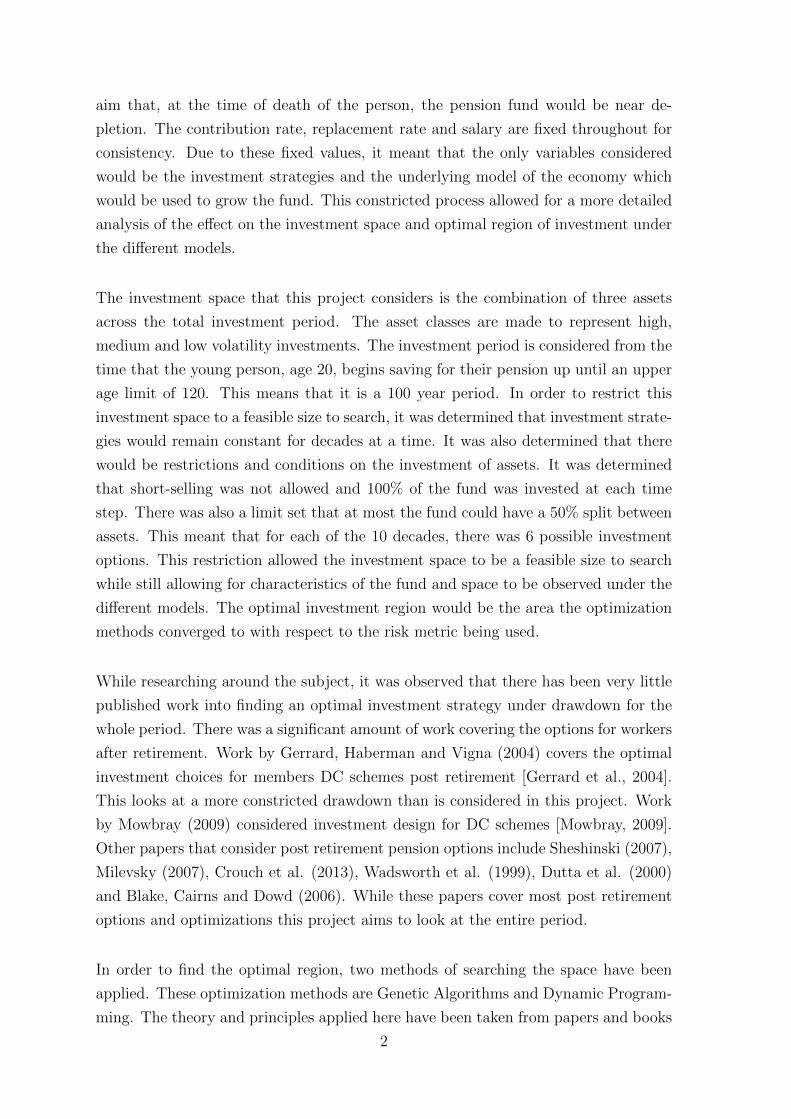
Introduction

This project aims to investigate the effect of changing the underlying model of the

economy on a pension fund through finding an optimal investment region for each

model. There will be two models being considered, the Wilkie Model and the cor-

related Geometric Brownian Motion (GBM). In order to investigate the effect, key

characteristics of the investment period shall be examined under each model, with the

optimal region of investments compared. For this project, the investment period will

be consider to be one period, from the start of saving until death. This is different

than the majority of approaches which will split the period into an accumulation and

de-cumulation stage. In these approaches, the accumulation stage would aim to grow

the pot as large as possible, which is not how this project approaches the optimization.

At the end of this project, a brief examination will be taken of the effect of splitting

the optimal region into these two stages.

The motivation behind this project is the increased drawdown flexibility introduced

in the 2014 UK Budget [HMT, 2014]. From April 2015 onwards, pensioners who have

pensions in a Defined Contribution (DC) scheme would be able to withdraw directly

from the fund, take a lump sum amount from the pot or buy an annuity with the

total savings. This change in the pension landscape gives more options and flexibility

to people approaching retirement [gov, 2015a]. Because of this, it was deemed im-

portant to investigate if the optimal region of investment strategies are comparable

across different models. The two models being considered here were chosen due to

the fact that the Wilkie Model can be described as a more complex model than the

GBM. This project will aim to investigate the similarity and differences observed in

the investment region under each model. For the course of this project only drawdown

shall be considered as the only income throughout retirement. This means that any

alternative income, including lump sum withdrawals and purchasing an annuity are

not included in any optimization procedure.

This project approaches the optimization of a pension scheme from a different angle.

Instead of considering the two stages, with the aim of growing the pot as large as

possible in the accumulation stage. It instead takes the region as a whole with the

1

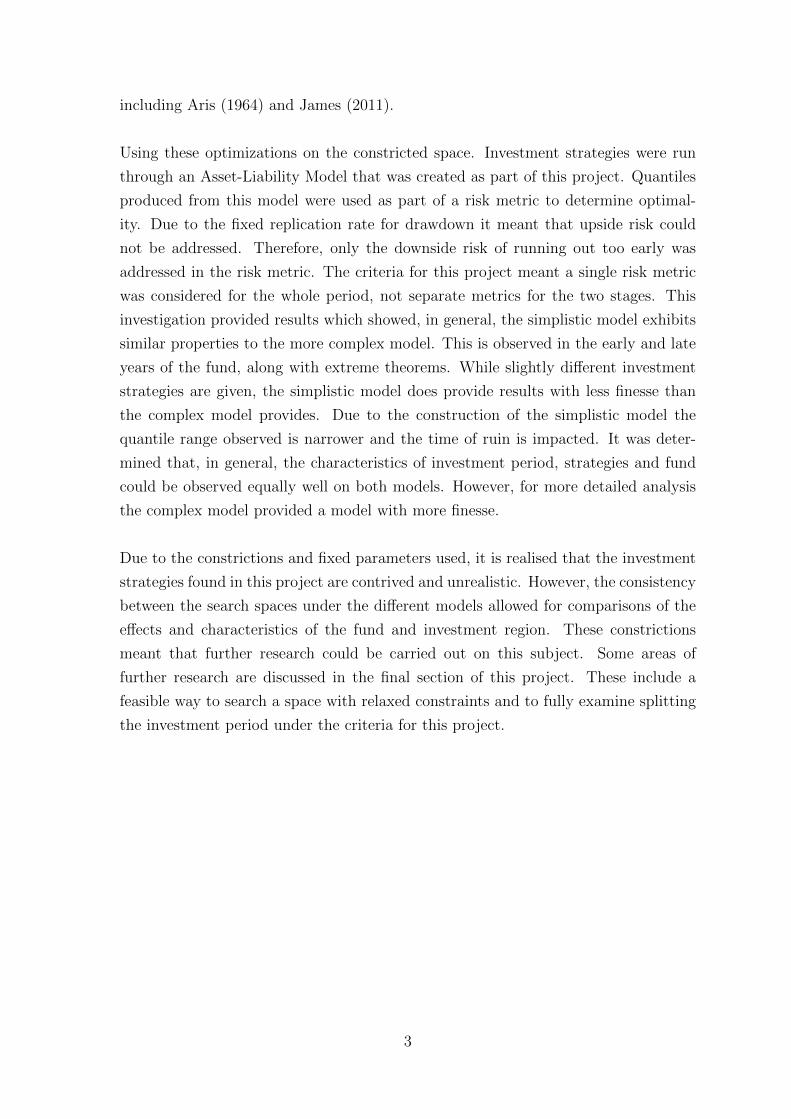
aim that, at the time of death of the person, the pension fund would be near de-

pletion. The contribution rate, replacement rate and salary are fixed throughout for

consistency. Due to these fixed values, it meant that the only variables considered

would be the investment strategies and the underlying model of the economy which

would be used to grow the fund. This constricted process allowed for a more detailed

analysis of the effect on the investment space and optimal region of investment under

the different models.

The investment space that this project considers is the combination of three assets

across the total investment period. The asset classes are made to represent high,

medium and low volatility investments. The investment period is considered from the

time that the young person, age 20, begins saving for their pension up until an upper

age limit of 120. This means that it is a 100 year period. In order to restrict this

investment space to a feasible size to search, it was determined that investment strate-

gies would remain constant for decades at a time. It was also determined that there

would be restrictions and conditions on the investment of assets. It was determined

that short-selling was not allowed and 100% of the fund was invested at each time

step. There was also a limit set that at most the fund could have a 50% split between

assets. This meant that for each of the 10 decades, there was 6 possible investment

options. This restriction allowed the investment space to be a feasible size to search

while still allowing for characteristics of the fund and space to be observed under the

different models. The optimal investment region would be the area the optimization

methods converged to with respect to the risk metric being used.

While researching around the subject, it was observed that there has been very little

published work into finding an optimal investment strategy under drawdown for the

whole period. There was a significant amount of work covering the options for workers

after retirement. Work by Gerrard, Haberman and Vigna (2004) covers the optimal

investment choices for members DC schemes post retirement [Gerrard et al., 2004].

This looks at a more constricted drawdown than is considered in this project. Work

by Mowbray (2009) considered investment design for DC schemes [Mowbray, 2009].

Other papers that consider post retirement pension options include Sheshinski (2007),

Milevsky (2007), Crouch et al. (2013), Wadsworth et al. (1999), Dutta et al. (2000)

and Blake, Cairns and Dowd (2006). While these papers cover most post retirement

options and optimizations this project aims to look at the entire period.

In order to find the optimal region, two methods of searching the space have been

applied. These optimization methods are Genetic Algorithms and Dynamic Program-

ming. The theory and principles applied here have been taken from papers and books

2

including Aris (1964) and James (2011).

Using these optimizations on the constricted space. Investment strategies were run

through an Asset-Liability Model that was created as part of this project. Quantiles

produced from this model were used as part of a risk metric to determine optimal-

ity. Due to the fixed replication rate for drawdown it meant that upside risk could

not be addressed. Therefore, only the downside risk of running out too early was

addressed in the risk metric. The criteria for this project meant a single risk metric

was considered for the whole period, not separate metrics for the two stages. This

investigation provided results which showed, in general, the simplistic model exhibits

similar properties to the more complex model. This is observed in the early and late

years of the fund, along with extreme theorems. While slightly different investment

strategies are given, the simplistic model does provide results with less finesse than

the complex model provides. Due to the construction of the simplistic model the

quantile range observed is narrower and the time of ruin is impacted. It was deter-

mined that, in general, the characteristics of investment period, strategies and fund

could be observed equally well on both models. However, for more detailed analysis

the complex model provided a model with more finesse.

Due to the constrictions and fixed parameters used, it is realised that the investment

strategies found in this project are contrived and unrealistic. However, the consistency

between the search spaces under the different models allowed for comparisons of the

effects and characteristics of the fund and investment region. These constrictions

meant that further research could be carried out on this subject. Some areas of

further research are discussed in the final section of this project. These include a

feasible way to search a space with relaxed constraints and to fully examine splitting

the investment period under the criteria for this project.

3

The Wilkie Model

In this chapter the Wilkie Model shall be introduced and some context will be given

for its use in this project. The total return indices will be given and finally, the mean

return and volatility across decades along with the correlation between indices shall

be examined.

Introduction and Background

The model being used in this project was provided by Professor Wilkie along with

the accompanying papers ”Yet More on a Stochastic Economic Model” parts 1 and 2

[Wilkie et al., 2011, Wilkie and Sahin, 2015]. Since the model is not the main area of

this project only some background will be given. These papers are used to update the

model which was first defined in the paper ”More on a Stochastic Investment Model

for Actuarial Use” in 1995 [Wilkie, 1995]. The papers update the inputs, bringing

them up-to-date and making slight adjustments to certain parts of the model through

updating and re-basing where necessary. They then go on to examine how the model

has faired in its predictions and look at the parameters of the model. In the main,

the original model is unchanged from 1995 by these papers for use in this project.

The Wilkie Model of the economy is a stochastic model based upon Box-Jenkins time

series models [Sahin et al., 2008]. The model has a cascading structure meaning that

there is a central value defining the state of the market. All other parameters come

from this central parameter [Fraysse, 2015]. This means that the model is stable in

times of crisis while providing acceptable forecasts of the future. The model used

in this project requires 14 initial conditions along with 35 parameters which give 13

outputs for the areas of the economy modelled. Parameters include means, standard

deviations, weighting factors and deviation from the mean [Wilkie et al., 2011]. These

parameters are input for all areas of the model. A number of areas include Retail

Prices, Wages, Share Dividends, long-term Bond Yields and a Base Rate as an example

of typical input areas. The weighting factors are used with respect to the inflation rate

calculated from the Retail Prices. This is due to the fact that inflation is the central

value in the cascading model. Some of the input parameters are with respect to an

Auto-Regressive Conditional Heteroskedasticity (ARCH) model which is introduced

4

as an alternative model for inflation [Sahin et al., 2008]. For this project only five of

the outputs are used. In the model, the parameters mostly come from least-squares

estimation meaning that they are unbias and linear with the actual models being

determined by either a stationary or integrated auto-regressive model of order one

(AR(1) or ARIMA(1,1,0)) [Sahin et al., 2008]. The structure of the model, as stated

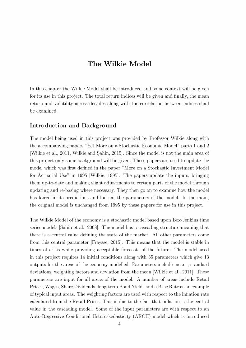
above is cascading, which is centred around inflation. A diagram of this cascading

model can be found below:

Figure 1: Cascading Structure of the Wilkie Model centred around Inflation

This diagram shows the cascade effect of the Wilkie Model for most of the major

components used in this project. While the basic concepts of the Wilkie Model follow

least-squares estimates and auto-regressive models there is some ARCH characteris-

tics for the residuals to account for fatter tails where necessary.

There is a fair amount of criticism of the Wilkie Model highlighting issues and areas

where it may fall short. Short-comings that are highlighted are that the model is

highly dependent on the initial parameters due to over parametrisation. There are

claims of biases in the estimations from inflation due to events in the market [Huber,

1995]. One criticism of the model which will be examined later is that in ”A Stochastic

Asset Model & Calibration for Long-term Financial Planning Purposes” [Hibbert

et al., 2001]. This shows that there there maybe an annual decrease in the standardised

volatility. There are also academic critics who highlight that the model does not hold

the no arbitrage or market efficiency theorem during times of stress [Fraysse, 2015].

There are upsides to using this model for this project. The outputs provide a good

basis for the total return indices used along with the access and simplicity of the

model. Since we are looking at pension fund investments over a long time span, the

Wilkie Model returning annual values was advantageous.

5

Total Return Indices

This section shall examine the total return indices used for this project. It was de-

cided to constrain the investment strategy to three investments in order to restrict the

search space. Effectively the three investments chosen are Equity, long-term Bonds

and Cash to replicate total returns indices with different risk-return profiles. The risk

considered when creating the index was the level of volatility produced by each of the

asset classes. When speaking about different levels of risk, the volatility produced is

used to distinguish between the high, median and low risk assets. The inflation index

has also been calculated to allow the salary and drawdown to grow with inflation.

The formula for the inflation index is:

Inflt = Inflt−1.exp{I(t)}

In this formula the index is given by Infl and I is the inflation output from the Wilkie

Model.

The formula for the total return index for equity is:

TRISt = TRISt−1.(P (t)+D(t))P (t−1)

Here the TRIS is the total return index for shares which consists of the price index

of shares, P , and the dividends paid at that time, D. This replicates higher risk of

volatile movements with higher expected return investments.

The formula for the total return index for long-term bonds is:

TRICt = TRICt−1.( 1C(t)

+1)( 1C(t−1))

The TRIC represents the total return index of Consol yield, Government Stocks,

which are assumed to pay an annual coupon of one. Even though perpetual stocks

are not available any more this represents a medium risk investment.

Finally, this is the formula to represent a cash total return index:

TRIBt = TRIBt−1. (1 +B(t))

This is not a true cash total return index since B represents short-term bond yield

which here shall represent a Cash total return Index. This is meant to represent a

safe, low risk investment.

6

All of the notation used can be found in the paper ”Yet More on a Stochastic Eco-

nomic Model: Part 1” [Wilkie et al., 2011]. The derivation of these formulae can be

found in Appendix 1.

Tax is not considered here since that goes beyond the scope of this project. Since

the aim of the project is to test robustness in optimal regions of investment strategies

across models it was important not to over complicate the inputs. Since the second

model used, which is defined in the next chapter, is calibrated to the outputs of these

indices it was deemed acceptable to ignore tax.

As discussed above, while these do not match the exact description or are totally

correct, the main idea is to test the robustness and characteristics of a region across

the models. It was decided that as long as the investments are consistent in returns,

volatility and correlation between assets across the models, it would be acceptable in

testing the robustness.

Mean Return, Volatility and Correlation

It was required that the a mean return, volatility and correlation between investment

options was found in order to calibrate the second model used in this project. To

achieve this, the average rate over 10 year periods was calculated for each simulation.

For the purpose of this project, it was deemed that 5000 simulations of the Wilkie

Model for 100 years will be used. This allowed for 5000 simulations of the value of

the pension fund across the investment period from the start of working life. It also

meant that it was possible to reduce the bias and error in the model due to the large

sample size. It implied that the sample mean return and volatility of the model could

be determined to a high degree of accuracy. Using this large number of simulations

meant that the bias cause by any outliers in the simulation was reduced. The graphs

of the simulations follow over the page.

7

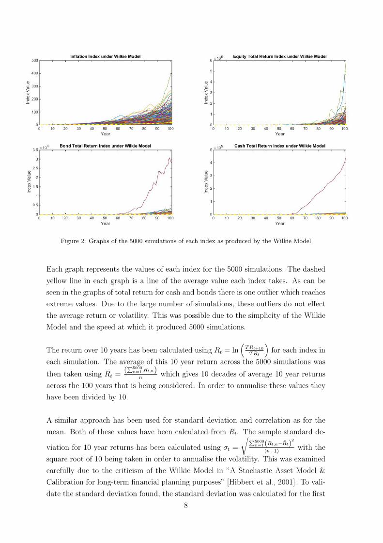
Figure 2: Graphs of the 5000 simulations of each index as produced by the Wilkie Model

Each graph represents the values of each index for the 5000 simulations. The dashed

yellow line in each graph is a line of the average value each index takes. As can be

seen in the graphs of total return for cash and bonds there is one outlier which reaches

extreme values. Due to the large number of simulations, these outliers do not effect

the average return or volatility. This was possible due to the simplicity of the Wilkie

Model and the speed at which it produced 5000 simulations.

The return over 10 years has been calculated using Rt = ln(TRt+10

TRt

)for each index in

each simulation. The average of this 10 year return across the 5000 simulations was

then taken using Rt =(∑5000

n=1 Rt,n)n

which gives 10 decades of average 10 year returns

across the 100 years that is being considered. In order to annualise these values they

have been divided by 10.

A similar approach has been used for standard deviation and correlation as for the

mean. Both of these values have been calculated from Rt. The sample standard de-

viation for 10 year returns has been calculated using σt =

√∑5000n=1(Rt,n−Rt)

2

(n−1)with the

square root of 10 being taken in order to annualise the volatility. This was examined

carefully due to the criticism of the Wilkie Model in ”A Stochastic Asset Model &

Calibration for long-term financial planning purposes” [Hibbert et al., 2001]. To vali-

date the standard deviation found, the standard deviation was calculated for the first

8

decade by hand. This used the same formula but individually calculating each part on

excel to validate the final value [Sto, 2015]. For both mean return and volatility, Rt has

been 10 year return for the index that was being calculated. When calculating the cor-

relation between the indices the formula used is ρi,j =∑5000

n=1(Rit,n−Ri

t)(Rjt,n−R

jt)√∑5000

n=1(Rit,n−Ri

t)2 ∑5000

n=1(Rjt,n−R

jt)

2 ,

where i, j = inflation, equity, bonds and cash. The values produced by these formulae

can be found in Appendix 2. It was observed from the output that after the first

20 years volatility and mean return remained consistent with correlation remaining

consistent throughout. In order to simplify the second model it was decided that a

single value, an average of the 10 decades, shall be used to reflect the annual return

and volatility. The implication and justification of this decision is discussed later in

the paper on the chapter on Optimization.

9

Correlated Geometric Brownian Motion

In this chapter the second model used in this project shall be introduced, the Geomet-

ric Brownian Motion. The creation and justification of choosing this model shall be

discussed followed by the mathematics behind the model and the use of the Cholesky

Decomposition. Finally, the calibration and validation process shall be covered.

Introduction

It was decided that the second model to be used in the project should be a simplistic

model in comparison with the Wilkie Model. Therefore, the Geometric Brownian

Motion (GBM) was selected since it is a simple log-normal model [epi, 2015].

The GBM can be used as a fundamental model of the economy since it produces

a basic exponential growth of assets. A stochastic process, Xt, follows a Brownian

Motion with the stochastic differential equation, dXt = µXtdt+ σXtdWt, where dWt

is a standard Brownian Motion, N(0, t) [Glasserman, 2003, p. 93:104]. Using Ito’s

formula it follows that the process has the form Xt = X0exp{(µ− 12σ2)t+σWt}, with

the full proof found in Appendix 3. This is the basic mathematics behind the second

model used in this project.

Using this Model

The use of the GBM comes from the methodology used previously in calculating the

10 year rate of return. From the form of the process in the previous section, Xt =

X0exp{(µ − 12σ2)t + σWt}, where Xt represents the annual total return index, TRt,

as calculated under the Wilkie Model. Rearranging this process gives ln(

TRt

TRt−1

)=

(µ− 12σ2)t+σWt which is an annual rate of return. Taking expectations and variance

of this formula gives E[ln(

TRt

TRt−1

)] = (µ− 1

2σ2)t which is an annualised average rate

of return, Rt. The variance is the volatility of the Wilkie Model, σt, for each decade.

This means that the formula used to model the annual total returns has the form:

TRt = TRt−1exp{R + σε}

In this formula R is the annual rate of return under the Wilkie Model. σ is the volatil-

ity under the Wilkie Model. Both of these values are the average for each decade,

10

calculated as R =∑10

t=1 Rt

10and σ =

∑10t=1 σt10

. Due to it being an annual total return, t

is 1 and the error term, ε, is distributed as a Multi-variate Normal, MVN(0, 1), with

correlation between indices. This is created using the Cholesky Decomposition.

The Multi-variate Normal (MVN) is created using the correlation matrix, ρ, which is

taken from the Wilkie Model. Since the errors in the GBM are normally distributed

with mean 0 and variance 1 the MVN is distributed N(0,Σ) where 0 is a vector of

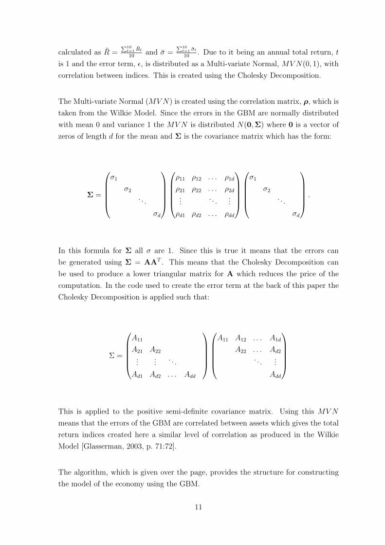
zeros of length d for the mean and Σ is the covariance matrix which has the form:

Σ =

σ1

σ2

. . .

σd

ρ11 ρ12 . . . ρ1d

ρ21 ρ22 . . . ρ2d

.... . .

...

ρd1 ρd2 . . . ρdd

σ1

σ2

. . .

σd

.

In this formula for Σ all σ are 1. Since this is true it means that the errors can

be generated using Σ = AAT . This means that the Cholesky Decomposition can

be used to produce a lower triangular matrix for A which reduces the price of the

computation. In the code used to create the error term at the back of this paper the

Cholesky Decomposition is applied such that:

Σ =

A11

A21 A22

......

. . .

Ad1 Ad2 . . . Add

A11 A12 . . . A1d

A22 . . . Ad2

. . ....

Add

This is applied to the positive semi-definite covariance matrix. Using this MVN

means that the errors of the GBM are correlated between assets which gives the total

return indices created here a similar level of correlation as produced in the Wilkie

Model [Glasserman, 2003, p. 71:72].

The algorithm, which is given over the page, provides the structure for constructing

the model of the economy using the GBM.

11

Algorithm 1 GBM model algorithm

for loop over each simulation, z doGenerate the correlated error for each simulation, errfor loop for each index, j do

Set the starting value for each index, S0(1, j)for loop over the time, i do

Generate the GBM simulations:Si,j,z = Si−1,j,z.exp{µj + σj.err}

The GBM grows the previous value of the index by the exponential ofthe mean and volatility multipled by the error term

end forend for

end for

This algorithm shows the logical progression of the function. The actual code used can

be found in Appendix 5. The code makes use of the ”SDETools” toolkit in MatLab

[Horchler, 2011]. The error is generated and correlated using the function mvnrnd

which applies the Cholesky Decomposition as described above.

Calibration and Validation

Since this project is based upon testing the robustness and characteristics of an opti-

mal investment region across different models it was deemed important that there is

a similarity across the models. For this reason it was important to validate that the

calibration of the GBM was consistent across the mean return, volatility and corre-

lation with that produced by the Wilkie Model. In order to validate the output of

the GBM, 4 areas were validated. These areas were the mean return, volatility and

correlation output from the total return indices in the GBM along with the correlation

between errors to confirm the source of the correlation. This was achieved through

similar methods as used when validating the output of the Wilkie Model. The out-

puts of the total return indices from the GBM was used to calculate 10 year rate of

returns which were then used to get the annualised average 10 year rate of returns

and volatility across the 5000 simulations. The correlation was also calculated from

this in the same manner as under the Wilkie Model. The correlation between error

terms was also examined over a large sample to determine that the correlation from

the errors was consistent with the correlation between the indices. For completeness,

the GBM was reproduced with independent standard normal distributions and the

correlation tested to confirm that the source of the correlation was the error term.

The graphs of the total return indices follow over the page.

12

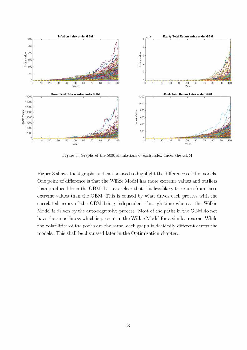
Figure 3: Graphs of the 5000 simulations of each index under the GBM

Figure 3 shows the 4 graphs and can be used to highlight the differences of the models.

One point of difference is that the Wilkie Model has more extreme values and outliers

than produced from the GBM. It is also clear that it is less likely to return from these

extreme values than the GBM. This is caused by what drives each process with the

correlated errors of the GBM being independent through time whereas the Wilkie

Model is driven by the auto-regressive process. Most of the paths in the GBM do not

have the smoothness which is present in the Wilkie Model for a similar reason. While

the volatilities of the paths are the same, each graph is decidedly different across the

models. This shall be discussed later in the Optimization chapter.

13

The Asset-Liability Model

In order for the pension fund to be accumulated and de-cumulated as required, it

meant that an Asset-Liability Model (ALM) had to be created. This chapter will

cover the creation and validation of the ALM.

Creating the Model

The objective of the ALM for this project is to allow a pension fund for a young

person to start saving from a given age and accumulate up to the Normal Retirement

Age (NRA). From the NRA a constant drawdown will be taken which will be a fixed

percentage of the final salary at retirement, this is known as the replacement rate.

This model was built for this project in order to control and understand where and

when the cash flows occurred. It was also created to meet the criteria of the project.

It was required that the entire investment area be considered as a whole. This ALM

allows for this by tackling accumulation and de-cumulation in the same model. The

project also only allows for a consistent drawdown to be taken from the pot until it

is depleted. This means that a number of options that are available to workers at

retirement have been omitted. These include the purchase of an annuity at retire-

ment or taking any of the pension pot as a lump sum. There are a number of papers

that discuss optimal pension options for post-retirement produces. However, these

assume the aim of the accumulation is to grow the pot as large as possible. In this

project, the aim of the whole process is to optimise a full strategy with the aim of go-

ing into drawdown. This allows for the characteristics of the full space to be examined.

A number of other assumptions and simplifications have also been made to allow for

the testing of the different models to be the main focus. A full list of the parameters

and constraints, along with the reasons behind choosing the values, can be found at

the end of this chapter. Some of the main parameters include constant pension con-

tribution rate, no early or late retirement, constant replacement rate, no promotions

or bonuses and an upper limit of life at 120 years old. The pension contributions

for this project are locked at 8% which is the minimum required by the government

by October 2018 [pas, 2015a]. With the aim of investigating the different models of

the economy the starting age is set at 20, along with the NRA at 65 with a salary of

14

£20,000. The fact that this is a fairly low income meant that the replacement rate was

fixed at 60% of the final salary which is normal according to Standard Life. In order

to simplify the optimization it was decided that there would be no salary inflation

through promotion and only RPI inflation would be considered to keep the buying

power of the salary constant.

The basics of the ALM are to accumulate the pension fund throughout the working

lifetime of a person. It then de-cumulates the fund through a drawdown pension

where a constant amount, with respect to inflation, is taken annually. The fund is

annually accumulated with respect to investment returns on an underlying model of

the economy with respect to the given investment strategy. This is run over a given

number of simulations from the model of the economy. The following algorithm gives

the structure of the ALM.

Algorithm 2 Asset-Liability Model algorithm

for loop for the accumulation period doEach contribution is inflated from the previous contribution with the annualrate of inflation.The fund is then accumulated up until NRA. This is done by accumulating thefund with investment returns and then adding that years contribution.

end forfor loop for the de-cumulation period do

The initial drawdown is calculated with respect to the salary inflated up toNRA.The drawdown for each time-step is then calculated using the previous draw-down amount and the annual inflation.The fund is then de-cumulated through time. This is done by accumulating thefund with respect to investment returns the taking the annual drawdownamount.

end for

It was decided that the fund would start off empty with the first contribution being

accounted for at the end of the first year. It was also decided that the drawdown was

received instantly at NRA. The code for the ALM written in MatLab can be found

in Appendix 5.

The investment returns in the ALM are accounted for using a weighted average on

the investment strategy. The returns are taken to be continuous so have the form:

exp{Weqi.ln(

TRISt

TRISt−1

)+Wbon.ln

(TRICt

TRICt−1

)+Wcas.ln

(TRIBt

TRIBt−1

)}

In this equation, TRIS, TRIC and TRIB are the total returns indices for equity,

bond and cash respectively. Wi represents the weights of the returns with respect to

15

the investment strategy, where i indicates the index the weight is relevant too.

The final function of the ALM is to count the time at which the fund goes negative

on a simulation. With the time at which the fund runs out a histogram is constructed

to display information about the life of the fund. This histogram and count of when

the fund goes negative is used in producing the risk metric which is used in the opti-

mization later.

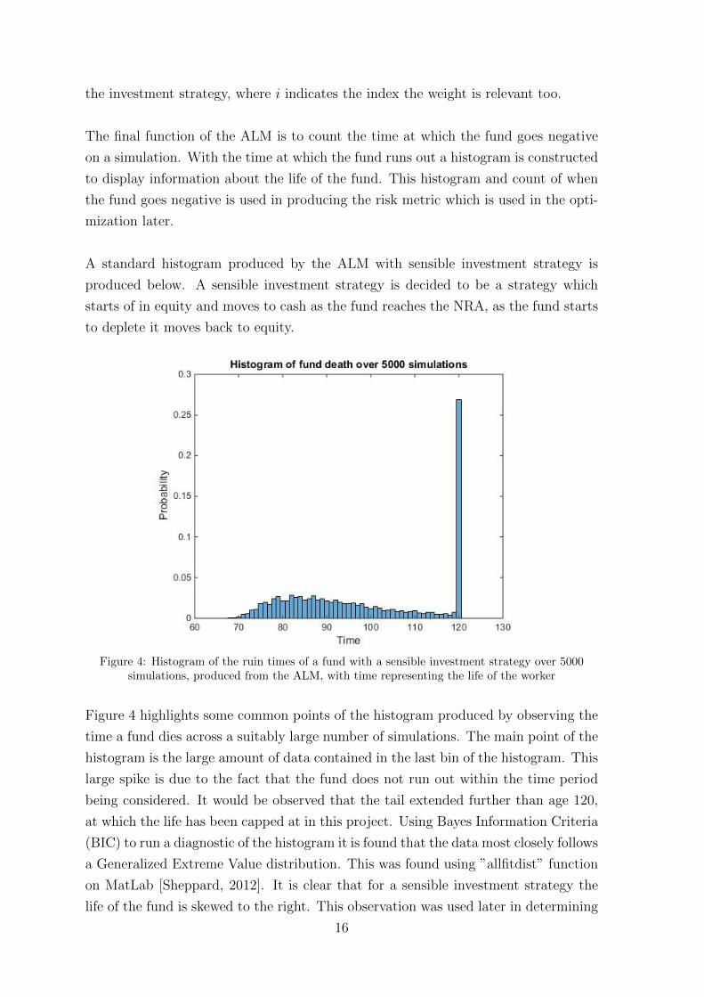
A standard histogram produced by the ALM with sensible investment strategy is

produced below. A sensible investment strategy is decided to be a strategy which

starts of in equity and moves to cash as the fund reaches the NRA, as the fund starts

to deplete it moves back to equity.

Figure 4: Histogram of the ruin times of a fund with a sensible investment strategy over 5000simulations, produced from the ALM, with time representing the life of the worker

Figure 4 highlights some common points of the histogram produced by observing the

time a fund dies across a suitably large number of simulations. The main point of the

histogram is the large amount of data contained in the last bin of the histogram. This

large spike is due to the fact that the fund does not run out within the time period

being considered. It would be observed that the tail extended further than age 120,

at which the life has been capped at in this project. Using Bayes Information Criteria

(BIC) to run a diagnostic of the histogram it is found that the data most closely follows

a Generalized Extreme Value distribution. This was found using ”allfitdist” function

on MatLab [Sheppard, 2012]. It is clear that for a sensible investment strategy the

life of the fund is skewed to the right. This observation was used later in determining

16

the risk metric for the optimization.

Calibration and Validation

In order to calibrate and validate the ALM, to confirm cash flows are falling at the

correct times, the model was first built using the algorithm in the previous section as

an aid. Once this model was created with flexible inputs it was then calibrated to a

basic model to ensure cash flows were being taken at the correct time.

The basic model of the ALM had three stages, each built on top of the previous, to

check different cash flows of the final model. This started with a simple deterministic

return with no inflation, then introduced inflation to the deterministic model and a

final full model dependent on a model of the economy for investment returns. The

deterministic return was set at 5% to confirm that the contributions and drawdowns

were taken at the correct time with respect to the annual growth of the fund. The

deterministic model with inflation was used to confirm that the salary, contributions

and drawdown were taking account of inflation at the correct time. The final full

model was used to validate that the ALM being used was providing correct consistent

values with respect to all values being fed into it. The ALM was checked with the

contrived models as they progressed with any alterations being made. This process

resulted in a fully calibrated and validated ALM which ran correctly.

Parameters and Constraints

This section will cover all the parameters and constraints that are relevant for search-

ing the space. The logic and reasoning behind choosing these values are also covered.

Since the main aim of this project was to consider the investment period as a whole,

it was deemed prudent to choose sensible values for all the inputs in the ALM. These

values would be kept constant throughout the process so that only the investment

strategy would be varied throughout the search.

The parameters in this project are considered to be the inputs to the ALM. These

include the start age of 20 years, the Normal Retirement Age (NRA) of 65 and the

final age considered as 120. In order to give a large investment period, the start age

was set at 20. This age was decided upon since it could cover both young people fin-

ishing apprenticeships, graduates from universities and people who had gone straight

into work from high school. 20 was decided to be a fair median age between these

groups. The NRA was set to 65 due to the fact it is a median for the age at which the

current state pension is received [gov, 2015b]. Previously, 65 was the NRA in the UK

17

but this has been phased out with no definite upper limit in most professions. It was

also determined that the life would be alive at NRA, since the aim of the project was

to examine the drawdown pension. The age 120 as an upper limit is being considered

due to the restriction of the life tables used. It is fairly common that 120 is considered

to be an upper limit for life.

Other parameters include the fixed salary of £20,000, the fixed contribution rate of

8% and the fixed replacement rate of 60%. This salary was decided upon since it rep-

resented an income which was considered low as it is below the nation average [ONS,

2013], but would keep an average family out of poverty [jrf, 2008]. It was important

that it wasn’t too low as it was decided that the salary would only grow with inflation

to keep the purchasing power, but would not grow with promotions or bonuses. The

contribution was set at 8% of the salary since it is a minimum rate required by the

government by 2018. The contribution will be made up from 4% from the employee,

3% from the employer and 1% from the government through tax breaks [pas, 2015a].

By keeping it constant at a low rate it avoided introducing lifestyle into the optimiza-

tion. In general a contribution rate would vary as the employee matured, with the

need of buying a house and supporting a family being removed from this project. The

replacement rate, the percentage of final salary received through drawdown, was set

at 60%. This is an industry standard where persons on a low income receive 60% of

the final salary as an income.

By fixing these parameters it meant that the only variables being considered by the

model was the underlying model of the economy and the investment strategy. This

allowed for a focus on searching the investment period for an optimal strategy and the

robustness of this strategy. The constraints on the inputs are discussed in the next

chapter concerning how the investment period has been constricted. By constricting

this region it allowed for the search region to be reduced to a feasible size.

18

Optimization Methods

This chapter will introduce the risk metric used to determine an optimal investment

strategy, what is considered to be optimal under this metric and other metrics that

could be considered. Once this has been introduced the different methods, Genetic

Algorithms and Dynamic Programming, for searching the space of possible investment

strategies shall be discussed.

Risk Metric

In general a risk metric is a quantifiable way to measure risk. The risk being consid-

ered in this project focuses on the risk of running out of income too early through

drawdown. It is also constrained by the fact this project does not want an excessively

large pot left at the death of the worker. If a large amount of money is left in the

pension pot it would imply the worker has not used the drawdown system to its full

advantage. It is assumed that the worker will not be leaving any money to beneficia-

ries which is why the pot must be as close to empty as possible. This project is only

considering altering investment strategy and not the contribution rate or drawdown

income. Therefore the risk being considered must aim to find an investment strategy

which provides a fund lifetime which will aim to be near depletion at the time of death

of a worker. This criteria was decided upon with the aim that the pensioner would

use their income to the full. A full optimization, which would allow for variable draw-

down and contribution rates is considered in the chapter on further research. This

uses Stochastic Control and would allow for the maximization of the workers income

and monetary needs through work and retirement.

To begin with, a measure for the workers life had to be decided upon. It was assumed

that the worker would survive up to the NRA (Normal Retirement Age) since only the

drawdown optimization was being considered. Using a life table provided by Standard

Life it was possible to create a density curve of the death of a life, alive at NRA. The

tables used were ”RMC00 with CMI 2013 M [1.5%] advanced improvements”. This

meant that there was a minimum improvement of 1.5% on the mortality rate through

time. These tables provided values of probability for dying at a given year and at

a given age. Using this information, a number of people alive at a given age was

19

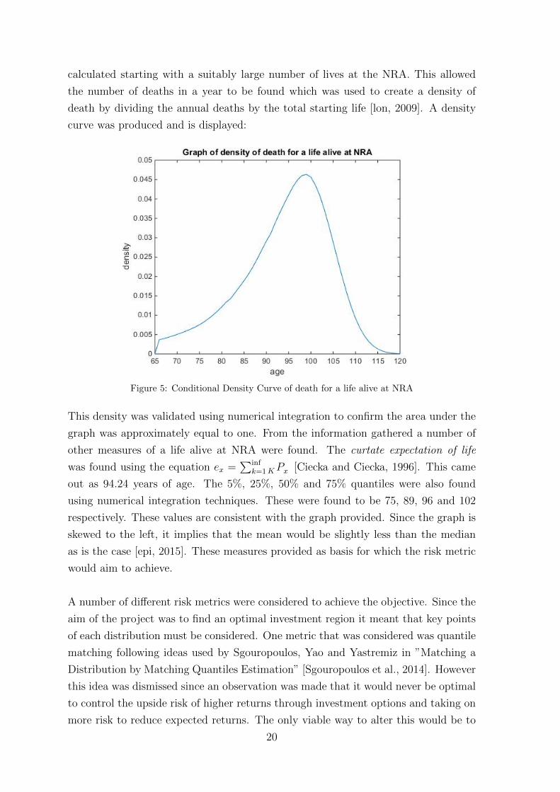
calculated starting with a suitably large number of lives at the NRA. This allowed

the number of deaths in a year to be found which was used to create a density of

death by dividing the annual deaths by the total starting life [lon, 2009]. A density

curve was produced and is displayed:

Figure 5: Conditional Density Curve of death for a life alive at NRA

This density was validated using numerical integration to confirm the area under the

graph was approximately equal to one. From the information gathered a number of

other measures of a life alive at NRA were found. The curtate expectation of life

was found using the equation ex =∑inf

k=1 PK x [Ciecka and Ciecka, 1996]. This came

out as 94.24 years of age. The 5%, 25%, 50% and 75% quantiles were also found

using numerical integration techniques. These were found to be 75, 89, 96 and 102

respectively. These values are consistent with the graph provided. Since the graph is

skewed to the left, it implies that the mean would be slightly less than the median

as is the case [epi, 2015]. These measures provided as basis for which the risk metric

would aim to achieve.

A number of different risk metrics were considered to achieve the objective. Since the

aim of the project was to find an optimal investment region it meant that key points

of each distribution must be considered. One metric that was considered was quantile

matching following ideas used by Sgouropoulos, Yao and Yastremiz in ”Matching a

Distribution by Matching Quantiles Estimation” [Sgouropoulos et al., 2014]. However

this idea was dismissed since an observation was made that it would never be optimal

to control the upside risk of higher returns through investment options and taking on

more risk to reduce expected returns. The only viable way to alter this would be to

20

alter the drawdown amount if excess cash has accumulated. Since this was constricted

for this project this method was rejected. It was also observed that the histogram of

fund life, as in figure 4, was skewed to the right while the density curve of death was

skewed to the left. This made it impractical to match quantiles of upside or downside

risk. Other metrics considered included work by Gerlach et al. (2012) [Gerlach et al.,

2012] where it was considered using their research into time varying quantiles with

respect to the aim in this project. However, since their work focuses on Value-at-Risk

it was deemed not to be applicable to this project.

Due to this observation it was decided that the risk metric that would be considered

would be matching the median of the funds life to the median of expected life. This

reduced the effect of the skew of the distributions. Optimality would also be indicated

through maximising the left hand quantiles of the fund, 5%, 10% and 25%. This would

allow a quantitative analysis of a strategy which would come close to being depleted

at a time close to the expected age of death of a pensioner. The effort to maximise

the lower quantiles meant that the downside risk of the pot running out before death

was also being addressed.

Methods of Optimization

This section covers the different methods of optimization used in the project. The

first method of optimization covered is the principles behind Genetic Algorithms (GA)

to search a space. The second method discussed is Dynamic Programming (DP), in

particular the Bellman Equations, to search the space. Two methods of optimization

are considered due to the different areas that are being searched and for completeness.

Before the methods of optimization are introduced the space that is being searched

must be defined. As discussed in the chapter on the Wilkie Model, there are 3 asset

classes for investment being considered. These represent a higher, medium and low

volatile risk investment options for a pension scheme. Since all other variables have

been constrained it allows for the change of investment strategy to be the only variable.

This results in the space to search which can be represented by the diagram which

follows over the page.

21

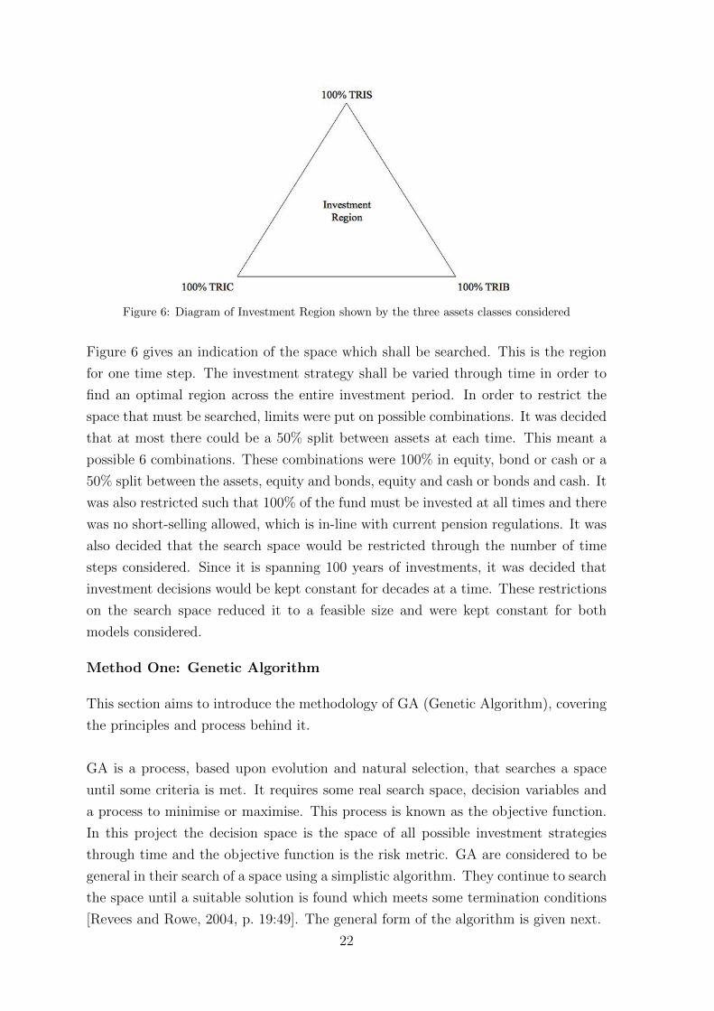
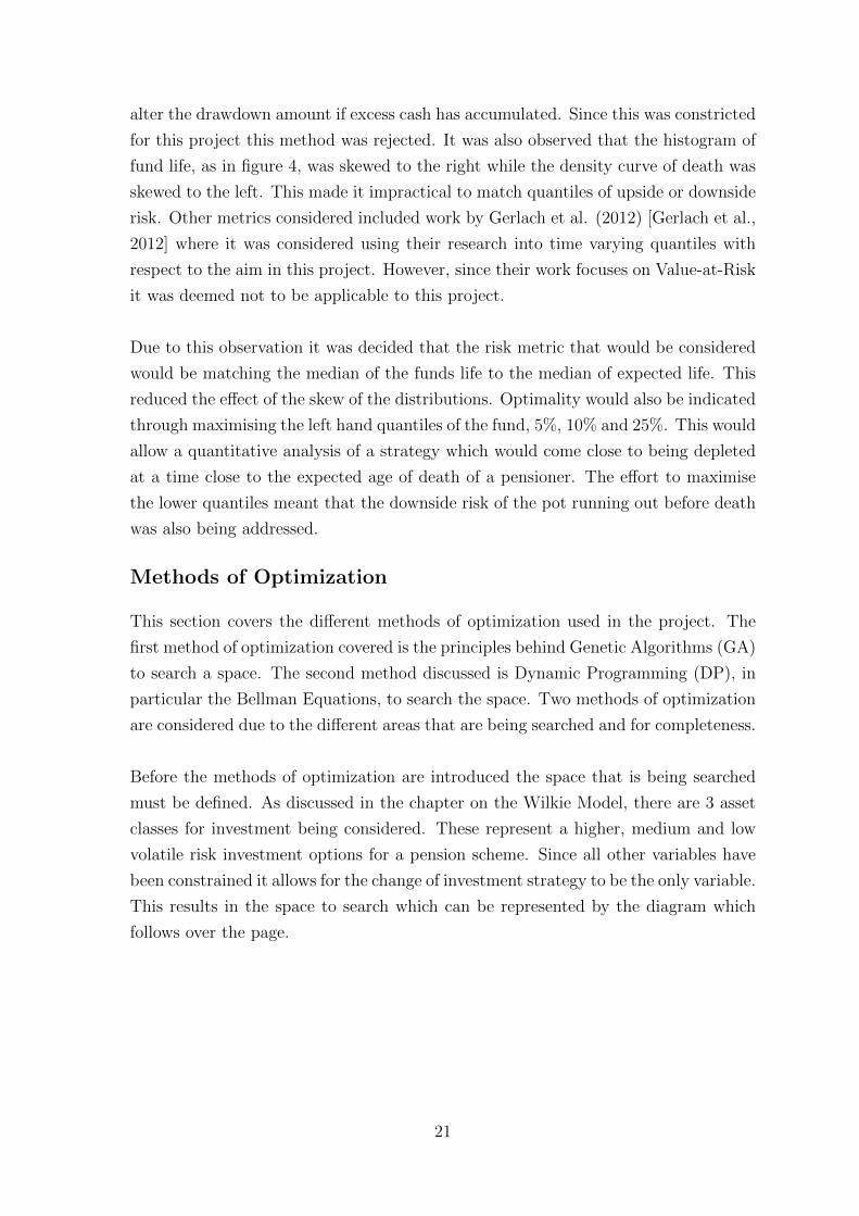
Figure 6: Diagram of Investment Region shown by the three assets classes considered

Figure 6 gives an indication of the space which shall be searched. This is the region

for one time step. The investment strategy shall be varied through time in order to

find an optimal region across the entire investment period. In order to restrict the

space that must be searched, limits were put on possible combinations. It was decided

that at most there could be a 50% split between assets at each time. This meant a

possible 6 combinations. These combinations were 100% in equity, bond or cash or a

50% split between the assets, equity and bonds, equity and cash or bonds and cash. It

was also restricted such that 100% of the fund must be invested at all times and there

was no short-selling allowed, which is in-line with current pension regulations. It was

also decided that the search space would be restricted through the number of time

steps considered. Since it is spanning 100 years of investments, it was decided that

investment decisions would be kept constant for decades at a time. These restrictions

on the search space reduced it to a feasible size and were kept constant for both

models considered.

Method One: Genetic Algorithm

This section aims to introduce the methodology of GA (Genetic Algorithm), covering

the principles and process behind it.

GA is a process, based upon evolution and natural selection, that searches a space

until some criteria is met. It requires some real search space, decision variables and

a process to minimise or maximise. This process is known as the objective function.

In this project the decision space is the space of all possible investment strategies

through time and the objective function is the risk metric. GA are considered to be

general in their search of a space using a simplistic algorithm. They continue to search

the space until a suitable solution is found which meets some termination conditions

[Revees and Rowe, 2004, p. 19:49]. The general form of the algorithm is given next.

22

Algorithm 3 GA algorithm

Choose an initial starting point to search from.Evaluate this information with respect to objective function.while Termination conditions not satisfied do

repeatif Use a combination to test space (Crossover) thenend ifif Use mutation to search surrounding space for better areas thenend ifReject or accept with respect to objective function

until optimal solution is foundSelect a new area to search

end while

From this algorithm it is clear to see the methodology of GA. It starts with an ini-

tial area to search against the objective function. Once this area is searched it uses

crossover and mutations to move through the space [sea, 2015].

Crossover in GA can be related to this project in testing combinations and deciding

whether or not different combinations provided better or worse results with respect

to the risk metric. Mutations have been considered in this project by changing an

investment option to test how it affects the metric.

This method has been applied in this project by taking the principles of the algorithm

above. In principle GA applies a heuristic algorithm, meaning it allows the user to

find the best solution through the search of a large space [Eiselt and Sandblom, 2012,

p. 175]. Heuristic methods allow for an optimum to be found, whereas exact methods

of search may just find a feasible region which is not optimal. An exact method which

was considered in this project was the Branch and Bound Method, where linear pro-

gramming is solved in a relaxed environment, honing in on a feasible solution given

the risk metric [Eiselt and Sandblom, 2012, p. 158]. This logic has been applied and

adapted in the searching the investment space. Suboptimal regions, with respect to

the risk metric, are rejected as the space is searched. In order to fully test the space

these suboptimal areas are only again considered in mutations in the GA.

The fact that an optimal investment region is being sought and not a strategy is

due to the method used. Since this project has restricted the space in such a way,

any single investment strategy would be illogical and unsound. Therefore the focus

is on the region of investment strategies that the optimization method hones in on.

Since the same method to search the space is applied to both models of the econ-

omy, the robustness of the region honed in on will be examined. It has also been

23

observed that numerical solutions attained by GA are unlikely to be exact predictions

[Forrest, 1993]. It is more common that GA provides insight into conditions of the

data, that is how the method is being applied in this project, when comparing models.

The actual logic for applying this method in this project is as follows. To begin with

the time for investments was split into two blocks of 50 years. The six combinations of

strategies, at each time, were ran through the Asset-Liability Model. This produced

the median and quantiles of the funds life to use as the risk metric. The best area was

honed in on with the rest being rejected as suboptimal. From there the algorithm

then moved to the next blocks of time, 33 year blocks. The process was repeated

using information gathered from the previous blocks. Again, after an initial search

of the space, the crossover was preformed by using combinations to hone in further.

Mutations were added to test a wider region and areas that had been rejected previ-

ously. This process continued through time blocks until 10 year blocks were reached.

The process of initial search based upon the results of the previous blocks were used

through out, using crossover and mutations to fully search the space. This process of

searching allowed the use of the principles of GA through time. It provided a com-

prehensive search which honed in on an optimal region of investment given the risk

metric.

Method Two: Dynamic Programming

This section aims to introduce the concept of DP (Dynamic Programming) along with

the principles and process behind it. It shall also discuss how it has been applied in

this project.

In particular, this project looks at Bellman’s principle of optimality and the equa-

tions connected to this [Bellman and Kalaba, 1965]. DP can be used to find optimal

solutions to sequential decision problems. A decision will be made upon current infor-

mation with respect to an objective. This is relatable to this project since a decision

must be made on an investment strategy for a decade which will affect the results of

the risk metric.

The framework for DP follows a straight forward process if there is a finite time hori-

zon, which there is in this case. Across a time dependent space, at each time step

or state, a decision must be made. The outcome of the decision made in this state

produces new information which is then carried forward to the next state. Each state

depends on the previous state and the decision that was made. This can be expressed

as transition probability, pss′ = P (St+1 = s′|St = s, at = a), where S is the state and

a is the decision that is made.

24

In the book ”Discrete Dynamic Programming” [Aris, 1964], the terms used in DP are

given. They are given over the page in the context of this project.

� State: The time steps across the lifetime of the investment. Here there are 10

states.

� Decision: The variable in the model. Here it is the choice of investment strategy

at each time step.

� Transformation: The decision at each state produces an output. This is seen in

this project when it is run through the ALM to gain the median and quantiles

of the fund given the investment strategy.

� Constraints : The constraints that are put on both the search space and the

decision variable. These include the 50% split between assets on the decision

variable and the decade time steps on the state.

� Objective Function: In this project this is represented by the risk metric which

determines optimality.

� Parameters : These are fixed constants. These may include the fixed Normal

Age of Retirement or fixed salary throughout.

This list gives an indication of the information needed for the process of DP and how

it is relatable to this project.

This project uses a form of DP introduced by Bellman in 1957. As the process moves

through states it is important to consider the final optimization and not focus on

achieving the best outcome at each time step. The Bellman Equations break the

problem in to a sum of smaller sub-problems with the aim to optimize the whole pro-

cess. It uses Markovian properties, meaning that only the current state is important

irrespective of past states [Judd, 1998, p. 409]. It is achieved through the Principle

of Optimality which states:

”An optimal policy has the property that whatever the initial state and initial

decision are, the remaining decisions must constitute an optimal policy with regard

to the state resulting from the first decision.”

This quote comes from ”Dynamic Programming and Modern Control Theory” [Bell-

man and Kalaba, 1965]. The application of this quote in the Bellman Equations is

that immediate optimality is combined with expected future optimality. The equa-

tions work recursively through time with a decision made at each state linked to the

25

next decision through these equations. The value function of the Bellman equations

has the form V (St) = maxat∈F(St)

f(St, at) + βV (St+1). This equation is the core of DP

and the principle behind it is applied in this project. In the equation, f(St, at) is

the function which indicates optimality in a state with β a weight on the value of

the next state. The F(St) represents the set of all possible decisions in the state.

The equation can also include the expectation of V (St+1) to account for a stochastic

decision process [James, 2011].

While considering DP, it is possible that issues known as ”the Curse of Dimensional-

ity” can arise. These issues come from the fact that there is a large number of choices

available at one point. This makes it too computationally expensive to explore every

future state. In order to correctly apply the Bellman Equations, all future states

must be considered. Due to the large dimensions this project is working in, this is

not possible. Even with the restricted space that is being searched, there are still

over 60 million combinations. If this search was relaxed to allow for assets to have

investments of 33% instead of 50% there would be over 10 billion combinations. This

exponential growth as the dimensions increase is the curse of dimensionality. [James,

2011]

The solution method to this equation is also recursive, given that the equation is

recursive. In this project there is a finite time horizon which means it is possible to

use ”Backward Dynamic Programming” starting from the last state. This requires

that the value function is found at each state as backwards induction is completed.

To apply this solution method, Policy Iteration techniques have been used. This re-

quires, from an initial starting point, DP is carried out reaching a feasible optimum.

At each stage, working backwards through time, a decision is made with respect to

the risk metric. This will search the space from the initial starting point. Then a

different starting point is considered and again DP reaches a feasible optimum and

so on. It can hone in on an optimum by using information gathered from previous

starting points. This would continue until an optimum is found. [James, 2011]

The principles of DP have been applied in this project. In the search of the investment

period while changing models, it is used as a secondary search method for complete-

ness. It is applied again when searching the effect of splitting the space. It uses the

risk metric as the objective function to search through time as the state. The invest-

ment strategy is being used as the decision process. The methodology used to find a

solution is policy iteration. A number of strategies are selected as different starting

points for the search. The optimization process works backwards through time to find

the optimal solution from the given starting point. This was done until convergence

26

and the optimal strategies are compared to select the best option. This searched

the space from various starting strategies, including extreme and sensible strategies

to preform a thorough search. This method of searching is known as Approximate

Dynamic Programming since it allows for sub-optimal, feasible regions to be found

using the concepts of DP. It makes it possible to work around the issues which arise

with the curse of dimensionality.

27

Changing the Model

This chapter will discuss the results obtained from the optimization under the two

models of the economy as defined previously. The differences and similarities in the

characteristics of the investment region found under each model shall be examined.

The key observations are summarised at the end of the chapter.

Results from Searching the Space

This section will discuss the optimal region of investment under each model separately,

along with the key observations. The exact method will be mentioned, however a more

detailed account of the process can be found in Appendix 4, along with tables showing

the output of the risk metric.

As defined in the criteria for this project, the investment period as a whole is being

considered. This will allow for an examination of the optimal strategy from the start

of the investment period right through until death. This is used as an alternative to

considering an optimal investment for accumulation which would be separate from the

de-cumulation period. The parameters and constraints are kept constant throughout,

when searching the space, and were defined in the Asset-Liability Model chapter. The

key parameters and constraints for the search are that the young person starting work

is aged 20 with an upper limit of life at 120. This gives the investment period of 100

years. The salary is locked at £20,000 which only accounts for inflation through the

RPI. The drawdown is fixed at a constant income of 60% of final salary. The reasoning

behind these values can also be found in the chapter on the Asset-Liability Model.

In order for consistency throughout, the Genetic Algorithm (GA) method shall be

used as an initial search method under both models of the economy. The Dynamic

Programming (DP) method shall then be applied for a final search of the space, from

a number of starting points, for completeness. This provides consistent parameters,

constraints and optimization methodology between the models. When discussing the

results the 5%, 10%, 25% and median shall be in the form [5%, 10%, 25%, median]

throughout for consistency.

Before the results and key observations are given, a brief oversight of the exact appli-

28

cation of each method shall be given.

The main process used to hone in on an optimal region for the full area is the GA

method. This uses the principles discussed in the section on the Genetic Algorithm.

As discussed in that chapter, the investment period was searched by moving through

blocks of time. Starting with two large blocks of 50 years the investment period was

searched, providing general results and observations of the attributes of the space.

Using the crossover process this allowed for unsuitable options to be discarded. These

discarded options would only be considered in later blocks of time as mutations to

search the space. This continued to hone in on a region by reducing the block sizes

until 10 year blocks were reached. Using observations from the previous time blocks

meant that the optimal region was found without a computationally expensive search.

The crossover technique was use to test if different combinations were optimal. By

adding in mutations of previously rejected investment options and combinations, the

search of the space was extended to test areas that had been rejected. Using both

these techniques under the GA method allowed for a thorough search of the invest-

ment period. This method was simplistic to run but honed in on a suitably optimal

region.

The second method used was the DP method discussed, in the section on Dynamic

Programming. Since it has been observed that the GA method provides a feasible

optimal region, it may not provide the global optimum. Therefore, for completeness,

it was decided that a second method should be applied to search the space. In order

to apply the DP method, initial starting strategies had to be decided upon. It was

viewed as prudent to start from a number of different extreme and sensible strategies.

The starting strategies decided upon were 100% and 50% split in each asset class

which provided six starting strategies and then another two sensible strategies. The

sensible strategies were the optimal found under the GA method and a basic strategy

which would have 100% in equity when the fund was at its smallest, moving to 100%

in cash when the fund was largest. The DP backwards iteration solution method was

applied to each of these strategies. If it was deem acceptable, it would be run again

from the strategy given from the first iteration. This allowed for an extensive search

of the space, on top of what had been achieved under the GA method.

In order to test optimality of an investment strategy, the strategy was ran through

the Asset-Liability Model. This produced quantiles of the fund’s ruin with respect to

the investment strategy and underlying model of the economy. All other variables of

the model were kept constant as defined above. Optimality was determined by the

risk metric which stated that the median should equal 96 with the lower quantiles of

29

the fund as high as possible. This process was the same under both models of the

economy. This allowed for consistency when checking the effect changing the model

has on the optimal region, and how robust this region is.

Results under the Wilkie Model

This section shall provide the key insights, observations and results under the Wilkie

Model. A full analysis of the process to arrive at these results can be found in

Appendix 4.

Optimal Region under Wilkie Model

This subsection will introduce the optimal region found under the Wilkie Model. A

brief description of the region is given. Using the methods of optimizations described,

an optimal region was found under the Wilkie Model. This optimal region has the

form:

� The first four decades contain 100% Equity.

� The fifth decade contained a 50% split between Equity and Cash

� The sixth decade contained a 50% split between Equity and Cash or Equity and

Bonds

� The seventh decade contained a combination of Cash and Bonds

� The last three decades contained 100% Equity or Bonds

The optimal region allows for flexibility in the sixth and seventh decades. Any in-

vestment strategies of this form provided a suitably optimal strategy. There was also

flexibility in the last 3 decades, it is discussed later in this section that these decades

have little effect on the median. It was found using the GA method. An exact strat-

egy of this form was used when applying the DP method to preform further searches

of the space. The results from using DP to further search the space showed that,

while there were alternative strategies that met the median, they were suboptimal

due to the fact that the quantiles were lower. The quantiles of 5%, 10%. 25% and

50% produced by the above strategy are [75, 78, 84, 96].

Key observations under Wilkie Model

This subsection covers the key observations and characteristics found while searching

the investment period. There are a number of characteristics discussed in this sec-

tion. The main discussion of these characteristics can be found in upcoming section,

30

discussion of results, which compares and contrasts results found under each model.

The first characteristic that was noted was that, with different criteria and risk met-

ric, investing 100% in equity for the entire investment period could be considered

optimal. This provided 5%, 10%, 25% and 50% quantiles as [76, 80, 89, 120], over

the 5000 simulations of the fund. This was considered to be an upper limit on what

the quantiles could achieve in this model. The reason behind this being considered an

upper limit is given in the upcoming discussion section which follows. This median

shows that at least 50% of the funds are active at the age 120. This would imply

these quantiles are as large as can be obtained. It is clear that, if the aim was to

grow the fund as large as possible across the whole investment period this is optimal.

It reinforced the view that quantile matching would not be logical or possible when

only considering altering the investment strategy. Upside risk of higher returns would

be reduced through poor investments which is suboptimal. As discussed in the Op-

timization chapter, the lower quantiles of death for a life alive at NRA were found

to be [75, 81, 89, 96]. By comparing the quantiles, it is observed that the quantiles

produced under this extreme strategy failed to meet the quantiles produced by the

death of a life. Since this extreme strategy produces quantiles which are considered

to be an upper bound, it implies that the quantiles of the fund will never meet those

of death. This was important to note during the search, as an assumption was made

that it was highly unlikely to match the quantiles, while matching the median. This

assumption was confirmed throughout the search when the upper limit on quantiles

was never reached in tandem with matching the medians.

The next characteristic observed from the search was the suboptimal effect of not

holding equity for the first 4 decades. Working through the space using crossover and

mutations highlighted this characteristic. Throughout the search of the investment

period, it was quickly noted that it was optimal to hold equity over anything else

in the early stages of the fund. A number of mutations were considered when using

the GA method to search but the majority were rejected since it caused the median

to fall short of 96. Another result of holding anything other than 100% equity in

the early stages was that the lower quantiles suffered. An example of this would be

holding 100% cash for the first decade while keeping the rest of the strategy as defined

above. This reduced the quantiles being considered to [75, 77, 82, 92]. There were

some investment options that could be held in the early years, however, by doing so

it reduced the flexibility of the optimal regions. This is highlighted by holding a 50%

split between cash and equity in the first decade. In order for the median to be met,

more equity must be held at later times to compensate. By holding 100% equity in the

sixth decade and 50% between cash and equity in the seventh decade to compensate,

31

the quantile values [75, 77, 83, 96] were produced. This shows that while the median

is met, the lower quantiles are impacted. The region of strategies which meet the

median with this criteria is also significantly reduced. This highlights that, while it is

possible to find an optimal strategy without equity in the early stages, it impacts neg-

atively on the optimal region. This characteristic was observed throughout the search.

A final characteristic observed was that the investment strategy in the later time peri-

ods have little impact on the median and quantiles being considered. It was observed

that both equity and bonds provided similar results to median and lower quantiles

when considered for the last 2 decades investments. This is due to the fact that by

age 100, or time 80, a large proportion of the funds are depleted. As observed un-

der the sensible investment strategy in Figure 4, approximately 70% of the funds are

depleted. This means that any investment options considered in these final time peri-

ods are only affecting a small number of simulations. It is likely that the median and

lower quantiles will be mostly dependent on funds which have ran out by this time.

It is also due to the fact that it would be expected that funds are relatively small

by this stage. There would have been 25 years worth of drawdown income taken out

with only the investment returns accounting for accumulation. When the fund is at

its largest, around about retirement, it would be expected that suboptimal strategies

have more impact at that point than at the end. Therefore, as it is important to

only consider equity in the early years, when the fund is smallest and growing, the

investment options in the last year have much less weight with respect to the risks

being considered. By observing this characteristic of the space it allowed for these

areas to be locked and only considered through mutations in the GA search method.

While searching the space with DP, after a feasible optimum region had been found

using GA, the characteristics of the early and late years of the fund were further

observed. It reiterated previous observations that it was suboptimal to not hold equity

in the early years and the final couple of decades had little effect on the median. Using

both methods provided a result which was considered to be the region of investments

which cover a global optimum.

Results under the Geometric Brownian Motion

This section will discuss the optimal region of investment under the Geometric Brow-

nian Motion (GBM). It shall also examine the characteristics of the search space

observed throughout the search. This section will not look to examine or discuss

the differences and similarities between the models in detail. The majority of that

discussion is held in the next section.

32

Optimal Region under GBM

This subsection will look at and give a brief discussion of the optimal regions of

investments under the GBM. Under the GBM the optimal region of investment was

found not to be unique. There were two regions which each contained strategies of

similar optimality. One of the regions was very similar to that of the region found

under the Wilkie Model. The first of the optimal regions has the form:

� The first five decades contain 100% Equity.

� The sixth and seventh decade containing a combination of Bonds and Cash

� The last three decades contained 100% Equity or Bonds

The second optimal region has the form:

� The first four decades contain 100% Equity

� The fifth decade contains a 50% split between Equity and Cash

� The sixth and seventh decades must contain some Equity which can be a combi-

nation with Bonds or Cash

� The eighth decade is flexible in that it can contain combinations or pure invest-

ments across Equity, Bonds and Cash

� The last two decades contained 100% Equity or Bonds

It was noticed that, while these regions are different, they exhibit some similar char-

acteristics. Both of these show that it is optimal to hold equity in the early years

of the fund, with differing degrees of flexibility in the middle years. They also both

show that the final years investments have similar characteristics. The first of the

optimal regions given has a narrower region of flexibility, but provides a slightly im-

proved optimal with respect to the quantiles. Both of these regions provide suitably

optimal strategies under the GBM. They were discovered using the GA approach.

The quantiles produced are approximately [72, 74, 81, 96] for both regions.

Key observations under GBM

This subsection will cover the key characteristics of the investment space observed un-

der the GBM. There are a number of characteristics considered, however, they shall

not be compared to those found under the Wilkie Model. This comparison will take

place in the next section, discussion of results.

33

The first characteristic examined, as before, was the effect of investing 100% in equity.

This was examined to measure the quantiles to gauge a possible upper limit. As with

the Wilkie Model it was observed that the quantiles for 100% equity investment fell

short of the quantiles of death. Under the GBM the quantiles were [72, 74, 83, 120].

These are not only less than the quantiles of death, but also fall short of the quantiles

observed under the Wilkie Model. This was used to give a possible upper limit of

quantiles which could be obtained when searching the space. By comparing these

quantiles to those produced in the optimal region it is observed that the quantiles are

easier to obtain at lower levels. This is due to the constructional differences between

the Wilkie Model and the GBM. Since the GBM is driven by independent normal

shocks [Glasserman, 2003, p.79], the inter quantile range is narrower which allows for

the extreme quantiles to be more easily obtained, as is evident here.

The next characteristic to be observed under the GBM was the impact on the median

and quantiles with respect to the investment in early years of the fund. This is similar

to the characteristic observed under the Wilkie Model. By considering alternative in-

vestments through the mutations in the GA search method, it was discovered that not

holding equity in the first four years was suboptimal and had a negative impact on the

quantiles. This observation was reiterated in the DP search where it was discovered

a number of singly optimal investment strategies. This meant there was no flexibility

in the strategy to form a region of optimum strategies. It was generally observed

that if a combination of equity was held at some point in the first three decades, a

strict strategy had to be followed throughout to meet the criteria of the risk metric.

In this context, a strict strategy is meant to mean that a strict process has to be

followed. In this case it was to hold almost 100% equity throughout to account for

this split in the early years. These strategies were noted, but discounted since there

was no improvement over the optimal regions found. They were also discounted due

to the fact the search space was rather naively constructed with the constriction of

investment options and spread of investments. It seemed illogical to rely on a single,

strict strategy where a region of strategies provided similar, if not better optimality,

with more flexibility and options to investigate the effects. Observing that it was

optimal to only hold equity for the first section of the investment period allowed for

a more focused search on the middle period, to hone in on the optimal region. The

early time periods were only considered as mutations.

The final characteristic observed under the GBM is the fact that the final time periods

have negligible impact on the median and lower quantiles. This will be due to the

same reason as discussed under the Wilkie Model. It would still be expected that as

the strategy moves through the investment period, it is more likely that the fund is

34

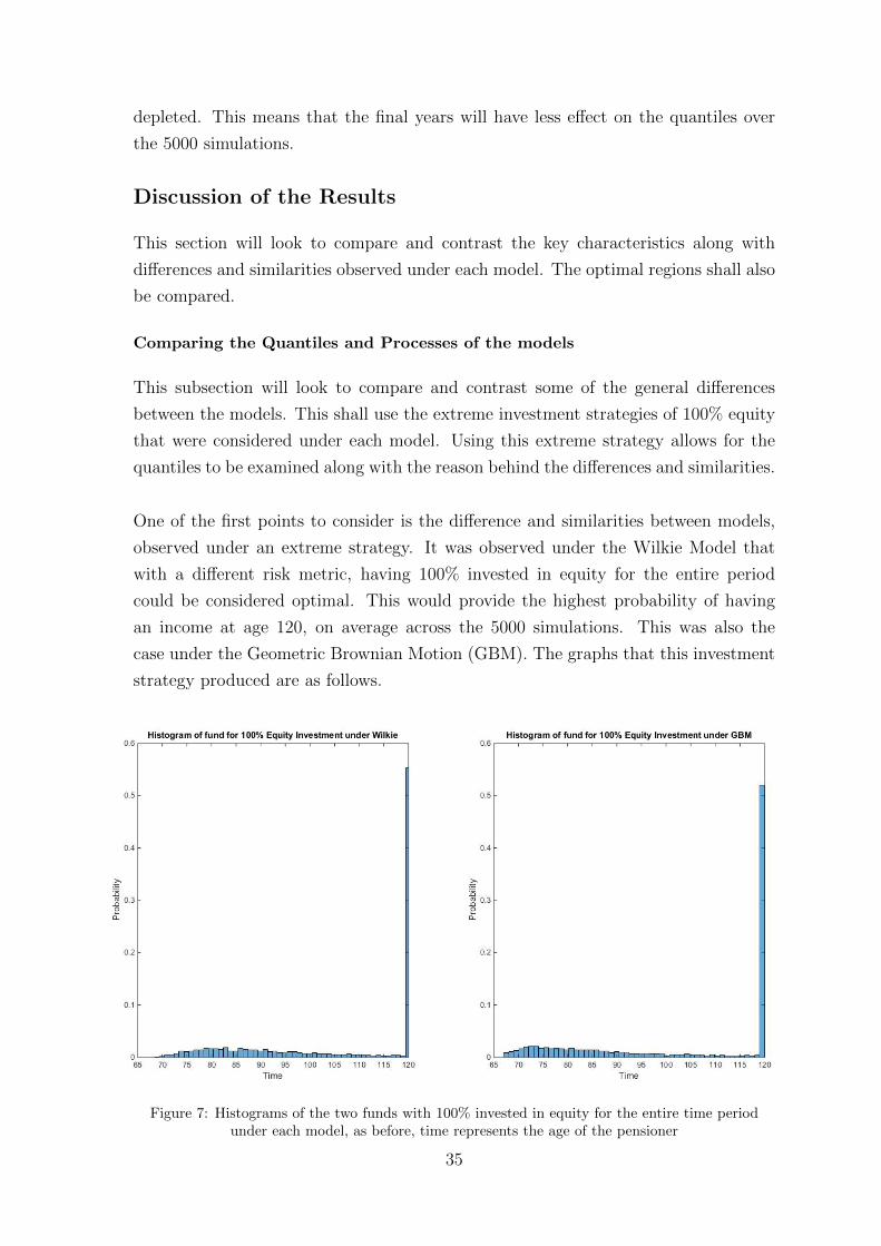
depleted. This means that the final years will have less effect on the quantiles over

the 5000 simulations.

Discussion of the Results

This section will look to compare and contrast the key characteristics along with

differences and similarities observed under each model. The optimal regions shall also

be compared.

Comparing the Quantiles and Processes of the models

This subsection will look to compare and contrast some of the general differences

between the models. This shall use the extreme investment strategies of 100% equity

that were considered under each model. Using this extreme strategy allows for the

quantiles to be examined along with the reason behind the differences and similarities.

One of the first points to consider is the difference and similarities between models,

observed under an extreme strategy. It was observed under the Wilkie Model that

with a different risk metric, having 100% invested in equity for the entire period

could be considered optimal. This would provide the highest probability of having

an income at age 120, on average across the 5000 simulations. This was also the

case under the Geometric Brownian Motion (GBM). The graphs that this investment

strategy produced are as follows.

Figure 7: Histograms of the two funds with 100% invested in equity for the entire time periodunder each model, as before, time represents the age of the pensioner

35

It is clear from figure 7 that both models have the same conclusion in this respect.

Both show that across the 5000 simulations there is approximately a 55% chance that

the fund will still have a positive value when the person is age 120. This is clearly

optimal if the fund as a whole was looking to be maximised, however, with respect

to the criteria for this project this is not optimal. While both funds have a similar

probability of being positive at age 120, the quantiles differ greatly.

The 5%, 10%, 25% and median under each model highlight a noticeable difference.

Under the Wilkie Model the quantiles are [76, 80, 89, 120] whereas under the GBM

they are [72, 74, 83, 120]. It is clear to see that the lower quantiles under the GBM

are smaller by a consistent amount than those in the Wilkie Model. This brings to

light the underlying differences in the models.

Another point observed from the quantiles produced under this extreme investment

strategy is with respect to the values observed. These higher quantiles observed were

considered to be an upper limit of what was achievable. Due to the skew to the right,

and the large amount of data held in the final bin, other quantiles could not surpass

these. This view was reinforced while searching the space, when no strategies pro-

vided better quantiles. By using this information, it meant that an upper limit could

be applied to what was achievable for the quantiles in the search. Since optimality

was being indicated in part by the quantiles, it meant that an indication of optimality

could be determined by how close the quantiles were to this upper limit. As seen from

the quantiles produced by the optimal region under the GBM it is possible to match

these. This would imply that this is the best optimal region under this search criteria.

Another observation of the quantiles was the consistency in range of quantiles between

the strategies under each model. The range between 5% and 25% under the Wilkie

Model was 13 years while the range under the GBM was 11 years under the extreme

equity strategy. Under both optimal regions the range was 9 years. Since the GBM

provides a narrower range in the extreme strategy, when it achieves the same range

in the optimal, this shows the consistency in the optimal region between the different

models.

As discussed in their respective chapters, the different models are driven by different

processes. The difference in processes is also evident in the graphs. Under the GBM

the years immediately after 65 are much more at risk of running out of money than

under the Wilkie Model. This is clearly the cause of the difference in quantiles but to

examine the cause of this, the accumulation period and driving period of each model

will have to be discussed.

36

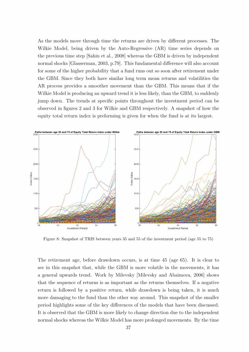
As the models move through time the returns are driven by different processes. The

Wilkie Model, being driven by the Auto-Regressive (AR) time series depends on

the previous time step [Sahin et al., 2008] whereas the GBM is driven by independent

normal shocks [Glasserman, 2003, p.79]. This fundamental difference will also account

for some of the higher probability that a fund runs out so soon after retirement under

the GBM. Since they both have similar long term mean returns and volatilities the

AR process provides a smoother movement than the GBM. This means that if the

Wilkie Model is producing an upward trend it is less likely, than the GBM, to suddenly

jump down. The trends at specific points throughout the investment period can be

observed in figures 2 and 3 for Wilkie and GBM respectively. A snapshot of how the

equity total return index is preforming is given for when the fund is at its largest.

Figure 8: Snapshot of TRIS between years 35 and 55 of the investment period (age 55 to 75)

The retirement age, before drawdown occurs, is at time 45 (age 65). It is clear to

see in this snapshot that, while the GBM is more volatile in the movements, it has

a general upwards trend. Work by Milevsky [Milevsky and Abaimova, 2006] shows

that the sequence of returns is as important as the returns themselves. If a negative

return is followed by a positive return, while drawdown is being taken, it is much

more damaging to the fund than the other way around. This snapshot of the smaller

period highlights some of the key differences of the models that have been discussed.

It is observed that the GBM is more likely to change direction due to the independent

normal shocks whereas the Wilkie Model has more prolonged movements. By the time

37

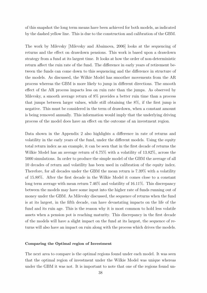
of this snapshot the long term means have been achieved for both models, as indicated

by the dashed yellow line. This is due to the construction and calibration of the GBM.

The work by Milevsky [Milevsky and Abaimova, 2006] looks at the sequencing of

returns and the effect on drawdown pensions. This work is based upon a drawdown

strategy from a fund at its largest time. It looks at how the order of non-deterministic

return affect the ruin rate of the fund. The difference in early years of retirement be-

tween the funds can come down to this sequencing and the difference in structure of

the models. As discussed, the Wilkie Model has smoother movements from the AR

process whereas the GBM is more likely to jump in different directions. The smooth

effect of the AR process impacts less on ruin rate than the jumps. As observed by

Milevsky, a smooth average return of 8% provides a better ruin time than a process

that jumps between larger values, while still obtaining the 8%, if the first jump is

negative. This must be considered in the term of drawdown, when a constant amount

is being removed annually. This information would imply that the underlying driving

process of the model does have an effect on the outcome of an investment region.

Data shown in the Appendix 2 also highlights a difference in rate of returns and

volatility in the early years of the fund, under the different models. Using the equity

total return index as an example, it can be seen that in the first decade of returns the

Wilkie Model has an average return of 6.75% with a volatility of 13.82%, across the

5000 simulations. In order to produce the simple model of the GBM the average of all

10 decades of return and volatility has been used in calibration of the equity index.

Therefore, for all decades under the GBM the mean return is 7.39% with a volatility

of 15.88%. After the first decade in the Wilkie Model it comes close to a constant

long term average with mean return 7.46% and volatility of 16.11%. This discrepancy

between the models may have some input into the higher rate of funds running out of

money under the GBM. As Milevsky discussed, the sequence of returns when the fund

is at its largest, in the fifth decade, can have devastating impacts on the life of the

fund and its ruin age. This is the reason why it is most common to hold less volatile

assets when a pension pot is reaching maturity. This discrepancy in the first decade

of the models will have a slight impact on the fund at its largest, the sequence of re-

turns will also have an impact on ruin along with the process which drives the models.

Comparing the Optimal region of Investment

The next area to compare is the optimal regions found under each model. It was seen

that the optimal region of investment under the Wilkie Model was unique whereas

under the GBM it was not. It is important to note that one of the regions found un-

38

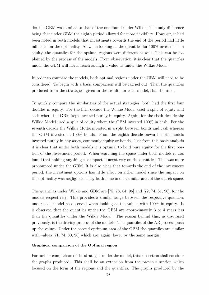
der the GBM was similar to that of the one found under Wilkie. The only difference

being that under GBM the eighth period allowed for more flexibility. However, it had

been noted in both models that investments towards the end of the period had little

influence on the optimality. As when looking at the quantiles for 100% investment in

equity, the quantiles for the optimal regions were different as well. This can be ex-

plained by the process of the models. From observation, it is clear that the quantiles

under the GBM will never reach as high a value as under the Wilkie Model.

In order to compare the models, both optimal regions under the GBM will need to be

considered. To begin with a basic comparison will be carried out. Then the quantiles

produced from the strategies, given in the results for each model, shall be used.

To quickly compare the similarities of the actual strategies, both had the first four

decades in equity. For the fifth decade the Wilkie Model used a split of equity and

cash where the GBM kept invested purely in equity. Again, for the sixth decade the

Wilkie Model used a split of equity where the GBM invested 100% in cash. For the

seventh decade the Wilkie Model invested in a split between bonds and cash whereas

the GBM invested in 100% bonds. From the eighth decade onwards both models

invested purely in any asset, commonly equity or bonds. Just from this basic analysis

it is clear that under both models it is optimal to hold pure equity for the first por-

tion of the investment period. When searching the space under both models it was

found that holding anything else impacted negatively on the quantiles. This was more

pronounced under the GBM. It is also clear that towards the end of the investment

period, the investment options has little effect on either model since the impact on

the optimality was negligible. They both hone in on a similar area of the search space.

The quantiles under Wilkie and GBM are [75, 78, 84, 96] and [72, 74, 81, 96], for the

models respectively. This provides a similar range between the respective quantiles

under each model as observed when looking at the values with 100% in equity. It

is observed that the quantiles under the GBM are approximately 3 or 4 years less

than the quantiles under the Wilkie Model. The reason behind this, as discussed

previously, is the driving process of the models. The quantiles of the AR process push

up the values. Under the second optimum area of the GBM the quantiles are similar

with values [71, 74, 80, 96] which are, again, lower by the same margin.

Graphical comparison of the Optimal region

For further comparison of the strategies under the model, this subsection shall consider

the graphs produced. This shall be an extension from the previous section which

focused on the form of the regions and the quantiles. The graphs produced by the

39

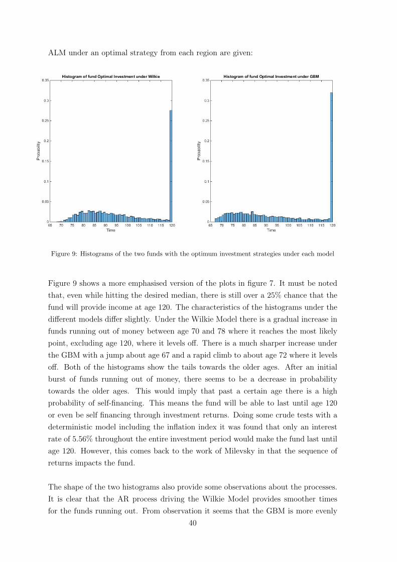
ALM under an optimal strategy from each region are given:

Figure 9: Histograms of the two funds with the optimum investment strategies under each model

Figure 9 shows a more emphasised version of the plots in figure 7. It must be noted

that, even while hitting the desired median, there is still over a 25% chance that the

fund will provide income at age 120. The characteristics of the histograms under the

different models differ slightly. Under the Wilkie Model there is a gradual increase in

funds running out of money between age 70 and 78 where it reaches the most likely

point, excluding age 120, where it levels off. There is a much sharper increase under

the GBM with a jump about age 67 and a rapid climb to about age 72 where it levels

off. Both of the histograms show the tails towards the older ages. After an initial

burst of funds running out of money, there seems to be a decrease in probability

towards the older ages. This would imply that past a certain age there is a high

probability of self-financing. This means the fund will be able to last until age 120

or even be self financing through investment returns. Doing some crude tests with a

deterministic model including the inflation index it was found that only an interest

rate of 5.56% throughout the entire investment period would make the fund last until

age 120. However, this comes back to the work of Milevsky in that the sequence of

returns impacts the fund.

The shape of the two histograms also provide some observations about the processes.

It is clear that the AR process driving the Wilkie Model provides smoother times

for the funds running out. From observation it seems that the GBM is more evenly

40

spread, with a less pronounced centre. It also means that the GBM has slightly larger

probabilities in the tails. From the large tails to the right under both models, it pro-

vides further evidence to the earlier point about the distribution of this data. It was

earlier theorised that the data could be modelled using a Generalised Extreme Value

distribution.

Conclusion of Comparison

There are a number of points to take away from the comparison of the different op-

timal regions of investment under the models. Firstly, from searching the space, it is

clear that both models provide similar results and analysis in the early and late years

of the strategies. There is consistency between the models in terms of quantiles. This

means that on the less sophisticated GBM, the quantiles will be consistently lower by

similar margins than those under the Wilkie Model. It is clear there could be some

issues when focusing on the middle of the investment strategy, if detailed analysis

was required. However, given the size of the space, both models will lead to a similar

optimal region. Both models do provide the same general shapes to the distribution,

with the Wilkie Model providing a smoother, more elegant shape. They both indicate

towards a distribution with a large right-hand tail.

The work by Milevsky [Milevsky and Abaimova, 2006] comes to the fore in some of

the observations. It is observed that the driving process of the models can affect

the investment strategy. Even though the models are calibrated to produce the same

mean return, volatility and correlation, once they have been ran through the ALM the

driving process takes affect. The movement of the indices under the different models

affects the ruin times of the funds under this different models. This can be explained

by considering the sequence of returns on a drawdown pension fund.

In general, it is possible to find an investment region under the simplistic GBM, which

would be similar to that under the Wilkie Model and satisfy the criteria. This region

shall also produce a similar range in quantiles and have the same characteristics.

However, the Wilkie Model does provide a more elegant model of the fund which

would provided better detailed analysis and statistical results. Therefore, in order to

hone in on an investment strategy and observe characteristics of the space, the highly

calibrated simplistic model will provide just as good results as the more complex

model.

41

Splitting the Time

This Chapter looks at the effect of splitting the period into accumulation and de-

cumulation. Instead of considering the time from the start of the working lifetime

until death, the optimal region shall now be searched by freezing one stage while

searching the other and vice versa. This is done using the simplistic method of Dy-

namic Programming (DP) as used as the second search method when considering the

investment period as a whole. A more complete and complex methodology for the

examination of the effect will be discussed.

In order to carry out this search some assumptions have been made. It was decided

that when one stage was frozen, an optimal strategy from the previous search would

be applied in that stage. In order to fully search the space of the side being consid-

ered, the Dynamic Programming (DP) method shall be applied. This uses the same

methodology as when using it for a second search method of the space as a whole.

This means it shall start from a number of different strategies. The backwards iter-

ation process is applied to search through time. The initial strategies used are the

same as before with 6 of the strategies being 100% and 50% split investment in the

asset class throughout the entire time. An optimal strategy will be used to explore

the surrounding space and then a basic sensible strategy, with equity when the fund

is at its smallest moving to cash as the fund reaches its largest. The search spaces

will be from 0 to 45 for the accumulation and from 45 to 100 for the de-cumulation

period. These times are with respect to the investment period, not the age of the

worker. As before, the investments will remain constant for decades, except for the 5

year periods around 45. Using these restrictions and the same criteria of the worker as

before it allowed for a basic investigation into effect of splitting the area. The Wilkie

Model was used as the underlying model of the economy.

Results and Discussion

The optimal strategy used was the one defined previously under the Wilkie Model.

For the accumulation period this meant the first four decades all in equity moving to

a 50% split between equity and cash for the last 5 years. The de-cumulation period

started with a 50% split between equity and cash for the first 15 years before moving

42

into cash for one decade then into bonds for the last three.

To begin the search the accumulation period was frozen while the de-cumulation pe-

riod searched. Starting from the optimal strategy and applying the DP methodology

altered some of the investments but kept it within the optimal region previously de-

fined. Starting from most of the other initial strategies converged to sub-optimal

strategies, meaning they met the median but the quantiles were too low. Some did

converge to optimal strategies within the previously defined region.

This search indicated that there would be no impact from freezing the accumulation

to search the de-cumulation period with the risk metric kept constant.

The next step was to freeze the de-cumulation and alter the accumulation. The same

techniques were used with the same initial strategies. As before, the process con-

verged to the optimal region. One anomaly was found which was that holding a 50%

split of equity and cash in the first decade could be considered optimal since there

was no impact on quantiles. However, as noted in the discussion of results when

changing the model, the resulting investment strategy was strict, consisting of more

equity. This was needed to produce higher returns to cover for the split in the first

period. Therefore, this was rejected since it reduced flexibility of the region without

improving the quantiles.

Since there was no difference in splitting the investment region while still applying

the same risk metric, this search reinforced previous observations about early and late

years in the period. While the fund was at its smallest, it was considered optimal to

hold equity. This observation allowed for more flexibility in the investment strategy

when the fund was at its largest. It was observed that if something other than equity

was held at these times, the flexibility of the investment strategy at its largest was

reduced since more equity would generally have to be held. The previous observation

of the flexibility in the final investment periods was also reinforced. When exploring

the de-cumulation period the flexibility in the final three periods was observed.

Effect of the Risk Metric

This search has been preformed using the same risk metric as previously defined.

That was, matching the median of the fund with the median of death for a life alive

at normal retirement age. This meant that the fund region as a whole was still re-

quired to be considered, even though only one half was being altered.

43

In order for a further, more complete investigation in the effect of splitting the target

period a new risk metric would have to be considered. This risk metric would have

to consist of two stages. It would require that some criteria was met for the accumu-

lation period which was compatible with some criteria for the de-cumulation stage.

Since this project was of the view that the fund aimed to be near depletion when the

worker died, this would have to be relevant in both risk metrics. Also, given that

only altering investment strategies were being considered, it would not make sense

for the metric of the accumulation to attempt to grow the fund as large as possible.

This comes back to a previous point made that it would never be optimal to con-

trol the upside risk of having too much money at death through investment options.

The only reasonable way to control this upside risk would be to consider increasing

the drawdown amount or saving less, if a variable contribution rate was being applied.

Due to the time constraints on this project it was not possible to investigate and apply

a risk metric which would accurately reflect the criteria given without considering the

investment period as a whole. However, a possible risk metric which could be applied

is discussed in the next chapter on Further Research.

44

Further Research

Due to the recent increase in flexibility for pensioners within the UK, with respect

to their pension options, there are a number of areas of further research that can be

considered. This chapter will discuss some of these areas, with respect to drawdown,

of further research and advancement.

Further research may include stochastic control could be applied to the problem en-

countered of dealing with the upside risk. A time consistent risk metric would need

to be considered to fully explore the effects of splitting the investment period.

Stochastic Control

The first area to look into for possible further research is the option of using stochas-

tic control in the optimization. This project constricted the optimization search to

the investment strategies. This meant that the upside of higher returns could not

be considered. Using stochastic control would allow for a more complete search of

the investment space. This project focused on the effect of changing the underlying

model of the economy but by applying stochastic control it would be possible to test

different aspects of investment strategies.

Stochastic control allows optimal feasible solutions to be found in complex systems.

By finding an optimal region of the entire space with all variables, including draw-

down and contributions, it would allow for further analysis. It could be used to find

the impact of having different investment strategies or different returns at certain

times. This would allow for a more complete understanding of the attributes of the

investment space. Stochastic control uses Dynamic Programming (DP) techniques

and could be applied to the space using stochastic control or optimal stopping.

Stochastic control involves finding the optimum for the next period using non-linear

programming. Instead of testing all the variables to find the optimum for the next

region, which can be exhaustive, it applies DP. A vector of all the variables is con-

sidered at each stage with respect to the given decision process, which here is the

risk metric. This vector of variables is incorporated into the DP equations using a

45

stochastic differential equation. This uses a look ahead approach to work forward

through time. If the time is continuous, Ito’s formula is applied. [Bertsekas, 1995,

p. 295]

Optimal stopping involves the decision maker determining whether or not it is opti-

mal to continue the search. As before it is underpinned using a stochastic differential

equation. The search is stopped if the stopping criteria is met with respect to the

value function. [Bertsekas, 1995, p. 168]

These are two methods of stochastic control which would allow for a more complete

optimization of the investment space. By altering the drawdown and contribution

amounts it would mean that the upside risk can also be considered when finding an

optimal region. In this project the downside risk of running out of money was the

focus in the risk metric, since it was not possible to attempt to reduce the upside

risk through the investment strategy. By using stochastic control it would allow for

varying drawdown to allow for a higher income, if the target was to be left with

as little as possible in the fund at death. As mentioned above, this more complete

optimization would also allow for investigation into inherent aspects of the investment

space. One aspect which could be considered under stochastic control would be the

life style choices of the worker. These choices were omitted in this project since it

would alter the contribution rate through time. This is one example of the possible

use of stochastic control to investigate other characteristics of the investment space,

along with how these changes affect an optimal region.

Time Consistent Risk Metric

A second area of further research, which would continue on from the content of this

project, would be to find a time consistent risk metric for splitting the investment

period.

Due to the time constraints on this project, the method applied when investigating

the effect of splitting the investment period is basic. In order to fully explore the

effect a time consistent risk metric would need to be created. If the aim of the risk

metric was consistent in that as little money would be left upon death as possible, a

risk metric for the accumulation period would have to account for this.

A basic method which could be applied would involve finding the optimal fund size

at retirement which would allow for a life to receive income until a given age. Under

different investment strategies, the fund could be discounted back with respect to the

46

drawdown to find this amount. This discount process would depend on the inflation

and the investment strategy. From there, the optimal accumulation could be found

with a given risk metric knowing that it had to attain a certain value. This would be

consistent with the optimal strategy for de-cumulation which would be determined

from the discount process.

Using this discount process would allow for an optimal strategy to be found over the

two stages. It would remain consistent in what it aims to do, due to the fact the

risk metric for accumulation depends on the value discovered in the de-cumulation.

This would allow for a different approach in finding the optimal region of investment

strategies. Observations and comparisons can be made of the new region, against that

of the one found when viewing the investment period as a whole.

47

Conclusion

This project has examined the effect on the optimal region of investment found under

two models of the economy. The two models considered are the Wilkie Model and

a correlated Geometric Brownian Motion (GBM). The investment period has been

considered as one entity when changing the underlying model of the economy. The

aim of the project was to discover if using a simplistic model, calibrated to a higher

level model, would provide a similar region of investments and to investigate the char-

acteristics of the models. In order to achieve this an Asset-Liability Model has been

created. The inputs were fixed for consistency when changing the models. An optimal

region of investments was honed in on using the principles behind two optimization

techniques, Genetic Algorithms and Dynamic Programming. Optimality was deter-

mined by a risk metric which met the criteria defined at the outset of the project. An

extension to this project was considered by splitting the region to examine the effect

this had on the investment strategy.

There have been a number of similarities observed under the different models. Under

both models it was observed that it was optimal to hold equity for the early years

of the fund as it accumulated. They both demonstrated that holding anything else

impacted negatively on the quantiles. Another similarity under both models was the

observation that the investment strategy in the last two decades had negligible im-

pact on the risk metric being considered. Finally, they both demonstrated similar

characteristics when holding 100% equity throughout the investment period. This

was suboptimal under the criteria in this project but highlighted the similar charac-

teristics across the models with this extreme strategy. There are differences observed

in the quantiles due to the construction of the models. Under the GBM the range of

quantiles was narrower which meant that the investment region found was not unique.

One of the key points to take away from this project is the effect of the driving pro-

cess of the underlying model. They models were created such that the mean return,

volatility and correlation between assets were consistent. However, it was observed

that the different driving processes of the models can have effect once they were

ran through the ALM. The independent normal shocks of the GBM were potentially

48

more damaging in the drawdown phase than the AR process driving the Wilkie Model.

This comes down to the sequencing of returns and their effects covered by Milevsky

[Milevsky and Abaimova, 2006].

The examination of splitting the model proved useful in examining the effect on early

and late time periods. However, due to time constraints it was not possible to pre-

form a full examination of this space. Methods were discussed to carry out a full

examination which involved discounting the fund back to the start of de-cumulation.

Overall, it was observed that using the simplistic model of the economy honed in on

a similar optimal region of investments for the fund. The models exhibited similar

key characteristics which produced similar sensible regions. However, it was observed

that, due to the narrower quantiles under the GBM, that to preform more sensitive

analysis of the fund, more exact results would be provided under the more complex

model. The simplistic model will still provide feasible and similar results but to a less

accurate degree.

49

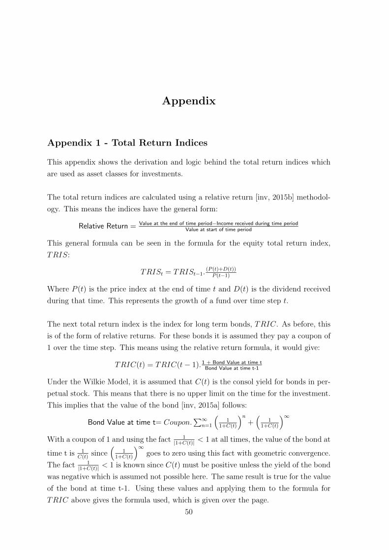
Appendix

Appendix 1 - Total Return Indices

This appendix shows the derivation and logic behind the total return indices which

are used as asset classes for investments.

The total return indices are calculated using a relative return [inv, 2015b] methodol-

ogy. This means the indices have the general form:

Relative Return = Value at the end of time period−Income received during time periodValue at start of time period

This general formula can be seen in the formula for the equity total return index,

TRIS:

TRISt = TRISt−1.(P (t)+D(t))P (t−1)

Where P (t) is the price index at the end of time t and D(t) is the dividend received

during that time. This represents the growth of a fund over time step t.

The next total return index is the index for long term bonds, TRIC. As before, this

is of the form of relative returns. For these bonds it is assumed they pay a coupon of

1 over the time step. This means using the relative return formula, it would give:

TRIC(t) = TRIC(t− 1).1 + Bond Value at time tBond Value at time t-1

Under the Wilkie Model, it is assumed that C(t) is the consol yield for bonds in per-

petual stock. This means that there is no upper limit on the time for the investment.

This implies that the value of the bond [inv, 2015a] follows:

Bond Value at time t= Coupon.∑∞

n=1

(1

1+C(t)

)n+(

11+C(t)

)∞With a coupon of 1 and using the fact 1

|1+C(t)| < 1 at all times, the value of the bond at

time t is 1C(t)

since(

11+C(t)

)∞goes to zero using this fact with geometric convergence.

The fact 1|1+C(t)| < 1 is known since C(t) must be positive unless the yield of the bond

was negative which is assumed not possible here. The same result is true for the value

of the bond at time t-1. Using these values and applying them to the formula for

TRIC above gives the formula used, which is given over the page.

50

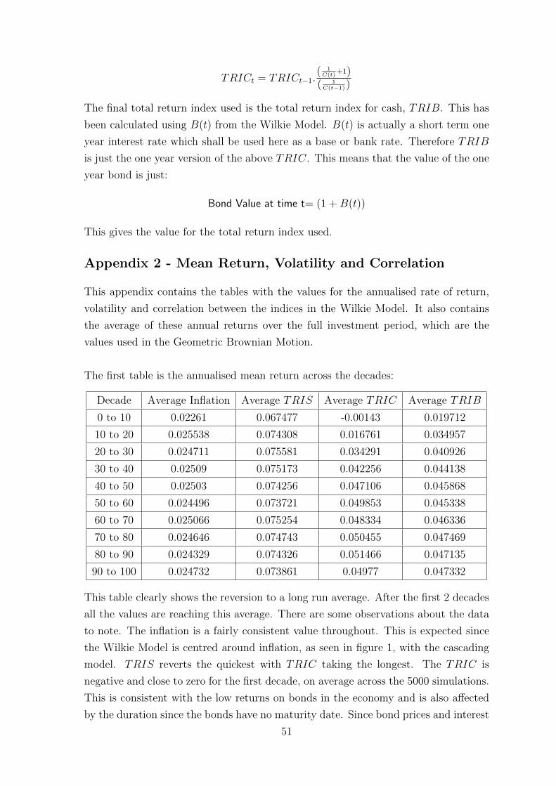
TRICt = TRICt−1.( 1C(t)

+1)( 1C(t−1))

The final total return index used is the total return index for cash, TRIB. This has

been calculated using B(t) from the Wilkie Model. B(t) is actually a short term one

year interest rate which shall be used here as a base or bank rate. Therefore TRIB

is just the one year version of the above TRIC. This means that the value of the one

year bond is just:

Bond Value at time t= (1 +B(t))

This gives the value for the total return index used.

Appendix 2 - Mean Return, Volatility and Correlation

This appendix contains the tables with the values for the annualised rate of return,

volatility and correlation between the indices in the Wilkie Model. It also contains

the average of these annual returns over the full investment period, which are the

values used in the Geometric Brownian Motion.

The first table is the annualised mean return across the decades:

Decade Average Inflation Average TRIS Average TRIC Average TRIB

0 to 10 0.02261 0.067477 -0.00143 0.019712

10 to 20 0.025538 0.074308 0.016761 0.034957

20 to 30 0.024711 0.075581 0.034291 0.040926

30 to 40 0.02509 0.075173 0.042256 0.044138

40 to 50 0.02503 0.074256 0.047106 0.045868

50 to 60 0.024496 0.073721 0.049853 0.045338

60 to 70 0.025066 0.075254 0.048334 0.046336

70 to 80 0.024646 0.074743 0.050455 0.047469

80 to 90 0.024329 0.074326 0.051466 0.047135

90 to 100 0.024732 0.073861 0.04977 0.047332

This table clearly shows the reversion to a long run average. After the first 2 decades

all the values are reaching this average. There are some observations about the data

to note. The inflation is a fairly consistent value throughout. This is expected since

the Wilkie Model is centred around inflation, as seen in figure 1, with the cascading

model. TRIS reverts the quickest with TRIC taking the longest. The TRIC is

negative and close to zero for the first decade, on average across the 5000 simulations.

This is consistent with the low returns on bonds in the economy and is also affected

by the duration since the bonds have no maturity date. Since bond prices and interest

51

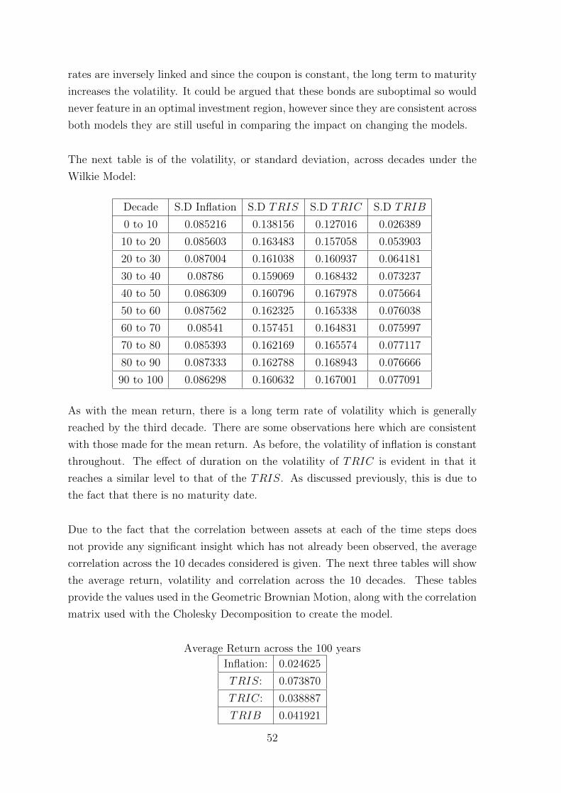
rates are inversely linked and since the coupon is constant, the long term to maturity

increases the volatility. It could be argued that these bonds are suboptimal so would

never feature in an optimal investment region, however since they are consistent across

both models they are still useful in comparing the impact on changing the models.

The next table is of the volatility, or standard deviation, across decades under the

Wilkie Model:

Decade S.D Inflation S.D TRIS S.D TRIC S.D TRIB

0 to 10 0.085216 0.138156 0.127016 0.026389

10 to 20 0.085603 0.163483 0.157058 0.053903

20 to 30 0.087004 0.161038 0.160937 0.064181

30 to 40 0.08786 0.159069 0.168432 0.073237

40 to 50 0.086309 0.160796 0.167978 0.075664

50 to 60 0.087562 0.162325 0.165338 0.076038

60 to 70 0.08541 0.157451 0.164831 0.075997

70 to 80 0.085393 0.162169 0.165574 0.077117

80 to 90 0.087333 0.162788 0.168943 0.076666

90 to 100 0.086298 0.160632 0.167001 0.077091

As with the mean return, there is a long term rate of volatility which is generally

reached by the third decade. There are some observations here which are consistent

with those made for the mean return. As before, the volatility of inflation is constant

throughout. The effect of duration on the volatility of TRIC is evident in that it

reaches a similar level to that of the TRIS. As discussed previously, this is due to

the fact that there is no maturity date.

Due to the fact that the correlation between assets at each of the time steps does

not provide any significant insight which has not already been observed, the average

correlation across the 10 decades considered is given. The next three tables will show

the average return, volatility and correlation across the 10 decades. These tables

provide the values used in the Geometric Brownian Motion, along with the correlation

matrix used with the Cholesky Decomposition to create the model.

Average Return across the 100 years

Inflation: 0.024625

TRIS: 0.073870

TRIC: 0.038887

TRIB 0.041921

52

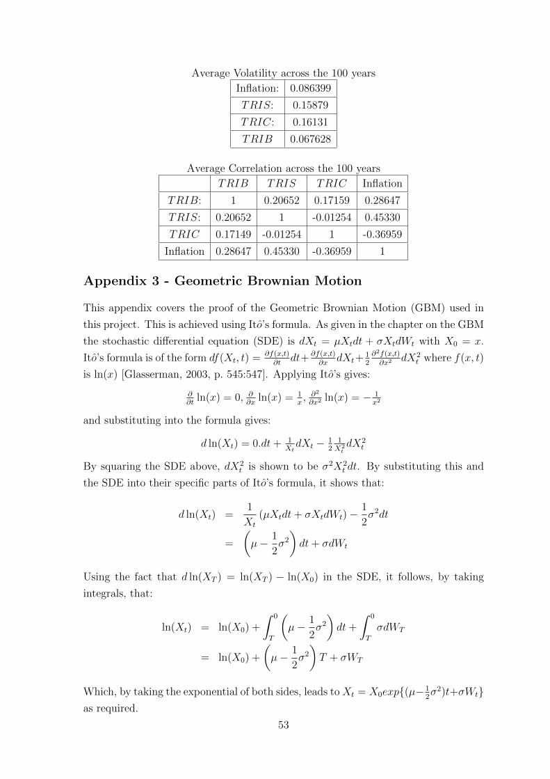
Average Volatility across the 100 years

Inflation: 0.086399

TRIS: 0.15879

TRIC: 0.16131

TRIB 0.067628

Average Correlation across the 100 years

TRIB TRIS TRIC Inflation

TRIB: 1 0.20652 0.17159 0.28647

TRIS: 0.20652 1 -0.01254 0.45330

TRIC 0.17149 -0.01254 1 -0.36959

Inflation 0.28647 0.45330 -0.36959 1

Appendix 3 - Geometric Brownian Motion

This appendix covers the proof of the Geometric Brownian Motion (GBM) used in

this project. This is achieved using Ito’s formula. As given in the chapter on the GBM

the stochastic differential equation (SDE) is dXt = µXtdt + σXtdWt with X0 = x.

Ito’s formula is of the form df(Xt, t) = ∂f(x,t)∂t

dt+ ∂f(x,t)∂x

dXt+12∂2f(x,t)∂x2

dX2t where f(x, t)

is ln(x) [Glasserman, 2003, p. 545:547]. Applying Ito’s gives:

∂∂t

ln(x) = 0, ∂∂x

ln(x) = 1x, ∂2

∂x2ln(x) = − 1

x2

and substituting into the formula gives:

d ln(Xt) = 0.dt+ 1XtdXt − 1

21X2

tdX2

t

By squaring the SDE above, dX2t is shown to be σ2X2

t dt. By substituting this and

the SDE into their specific parts of Ito’s formula, it shows that:

d ln(Xt) =1

Xt

(µXtdt+ σXtdWt)−1

2σ2dt

=

(µ− 1

2σ2

)dt+ σdWt

Using the fact that d ln(XT ) = ln(XT ) − ln(X0) in the SDE, it follows, by taking

integrals, that:

ln(Xt) = ln(X0) +

∫ 0

T

(µ− 1

2σ2

)dt+

∫ 0

T

σdWT

= ln(X0) +

(µ− 1

2σ2

)T + σWT

Which, by taking the exponential of both sides, leads toXt = X0exp{(µ− 12σ2)t+σWt}

as required.

53

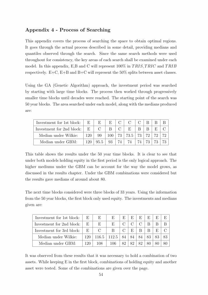
Appendix 4 - Process of Searching

This appendix covers the process of searching the space to obtain optimal regions.

It goes through the actual process described in some detail, providing medians and

quantiles observed through the search. Since the same search methods were used

throughout for consistency, the key areas of each search shall be examined under each

model. In this appendix, E,B and C will represent 100% in TRIS, TRIC and TRIB

respectively. E+C, E+B and B+C will represent the 50% splits between asset classes.

Using the GA (Genetic Algorithm) approach, the investment period was searched

by starting with large time blocks. The process then worked through progressively

smaller time blocks until decades were reached. The starting point of the search was

50 year blocks. The area searched under each model, along with the medians produced

are:

Investment for 1st block: E E E C C C B B B

Investment for 2nd block: E C B C E B B E C

Median under Wilkie: 120 99 100 73 73.5 73 72 72 72

Median under GBM: 120 95.5 93 74 74 74 73 73 73

This table shows the results under the 50 year time blocks. It is clear to see that

under both models holding equity in the first period is the only logical approach. The

higher mediums under the GBM can be account for the way the model grows, as

discussed in the results chapter. Under the GBM combinations were considered but

the results gave medians of around about 80.

The next time blocks considered were three blocks of 33 years. Using the information

from the 50 year blocks, the first block only used equity. The investments and medians

given are:

Investment for 1st block: E E E E E E E E E

Investment for 2nd block: E E E C C C B B B

Investment for 3rd block: E C B C E B B E C

Median under Wilkie: 120 116.5 112.5 84 84 84 83 83 83

Median under GBM: 120 108 106 82 82 82 80 80 80

It was observed from these results that it was necessary to hold a combination of two

assets. While keeping E in the first block, combinations of holding equity and another

asset were tested. Some of the combinations are given over the page.

54

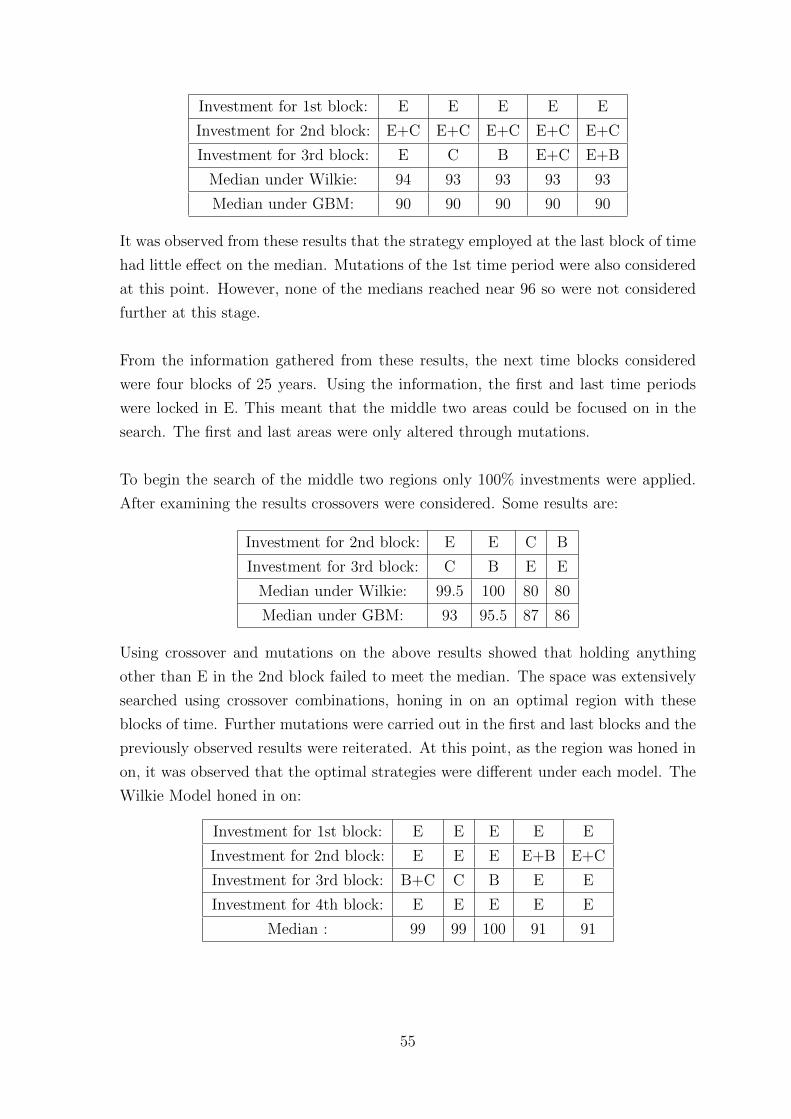
Investment for 1st block: E E E E E

Investment for 2nd block: E+C E+C E+C E+C E+C

Investment for 3rd block: E C B E+C E+B

Median under Wilkie: 94 93 93 93 93

Median under GBM: 90 90 90 90 90

It was observed from these results that the strategy employed at the last block of time

had little effect on the median. Mutations of the 1st time period were also considered

at this point. However, none of the medians reached near 96 so were not considered

further at this stage.

From the information gathered from these results, the next time blocks considered

were four blocks of 25 years. Using the information, the first and last time periods

were locked in E. This meant that the middle two areas could be focused on in the

search. The first and last areas were only altered through mutations.

To begin the search of the middle two regions only 100% investments were applied.

After examining the results crossovers were considered. Some results are:

Investment for 2nd block: E E C B

Investment for 3rd block: C B E E

Median under Wilkie: 99.5 100 80 80

Median under GBM: 93 95.5 87 86

Using crossover and mutations on the above results showed that holding anything

other than E in the 2nd block failed to meet the median. The space was extensively

searched using crossover combinations, honing in on an optimal region with these

blocks of time. Further mutations were carried out in the first and last blocks and the

previously observed results were reiterated. At this point, as the region was honed in

on, it was observed that the optimal strategies were different under each model. The

Wilkie Model honed in on:

Investment for 1st block: E E E E E

Investment for 2nd block: E E E E+B E+C

Investment for 3rd block: B+C C B E E

Investment for 4th block: E E E E E

Median : 99 99 100 91 91

55

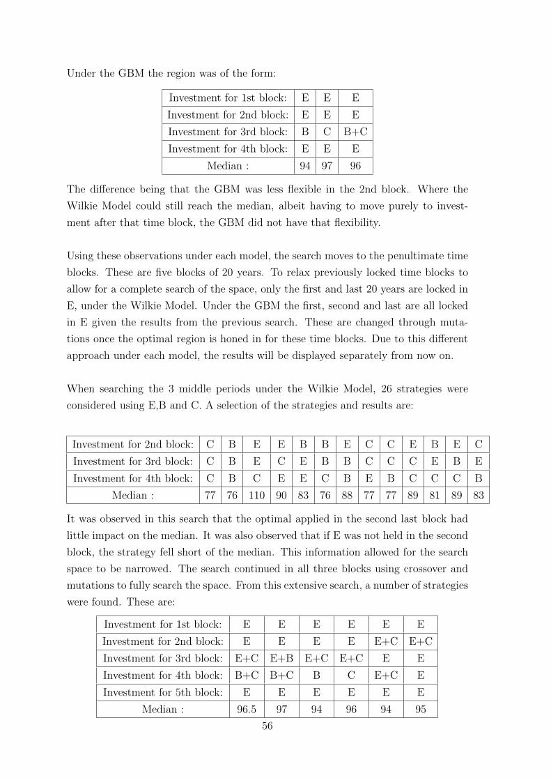
Under the GBM the region was of the form:

Investment for 1st block: E E E

Investment for 2nd block: E E E

Investment for 3rd block: B C B+C

Investment for 4th block: E E E

Median : 94 97 96

The difference being that the GBM was less flexible in the 2nd block. Where the

Wilkie Model could still reach the median, albeit having to move purely to invest-

ment after that time block, the GBM did not have that flexibility.

Using these observations under each model, the search moves to the penultimate time

blocks. These are five blocks of 20 years. To relax previously locked time blocks to

allow for a complete search of the space, only the first and last 20 years are locked in

E, under the Wilkie Model. Under the GBM the first, second and last are all locked

in E given the results from the previous search. These are changed through muta-

tions once the optimal region is honed in for these time blocks. Due to this different

approach under each model, the results will be displayed separately from now on.

When searching the 3 middle periods under the Wilkie Model, 26 strategies were

considered using E,B and C. A selection of the strategies and results are:

Investment for 2nd block: C B E E B B E C C E B E C

Investment for 3rd block: C B E C E B B C C C E B E

Investment for 4th block: C B C E E C B E B C C C B

Median : 77 76 110 90 83 76 88 77 77 89 81 89 83

It was observed in this search that the optimal applied in the second last block had

little impact on the median. It was also observed that if E was not held in the second

block, the strategy fell short of the median. This information allowed for the search

space to be narrowed. The search continued in all three blocks using crossover and

mutations to fully search the space. From this extensive search, a number of strategies

were found. These are:

Investment for 1st block: E E E E E E

Investment for 2nd block: E E E E E+C E+C

Investment for 3rd block: E+C E+B E+C E+C E E

Investment for 4th block: B+C B+C B C E+C E

Investment for 5th block: E E E E E E

Median : 96.5 97 94 96 94 95

56

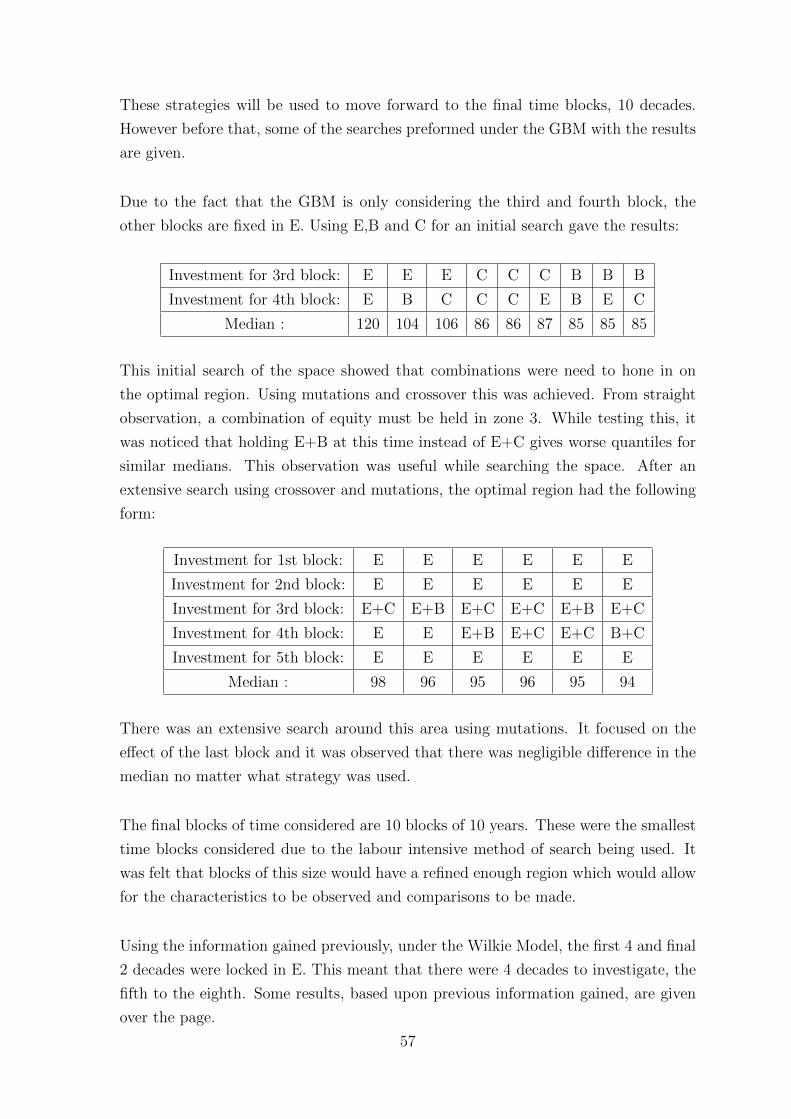
These strategies will be used to move forward to the final time blocks, 10 decades.

However before that, some of the searches preformed under the GBM with the results

are given.

Due to the fact that the GBM is only considering the third and fourth block, the

other blocks are fixed in E. Using E,B and C for an initial search gave the results:

Investment for 3rd block: E E E C C C B B B

Investment for 4th block: E B C C C E B E C

Median : 120 104 106 86 86 87 85 85 85

This initial search of the space showed that combinations were need to hone in on

the optimal region. Using mutations and crossover this was achieved. From straight

observation, a combination of equity must be held in zone 3. While testing this, it

was noticed that holding E+B at this time instead of E+C gives worse quantiles for

similar medians. This observation was useful while searching the space. After an

extensive search using crossover and mutations, the optimal region had the following

form:

Investment for 1st block: E E E E E E

Investment for 2nd block: E E E E E E

Investment for 3rd block: E+C E+B E+C E+C E+B E+C

Investment for 4th block: E E E+B E+C E+C B+C

Investment for 5th block: E E E E E E

Median : 98 96 95 96 95 94

There was an extensive search around this area using mutations. It focused on the

effect of the last block and it was observed that there was negligible difference in the

median no matter what strategy was used.

The final blocks of time considered are 10 blocks of 10 years. These were the smallest

time blocks considered due to the labour intensive method of search being used. It

was felt that blocks of this size would have a refined enough region which would allow

for the characteristics to be observed and comparisons to be made.

Using the information gained previously, under the Wilkie Model, the first 4 and final

2 decades were locked in E. This meant that there were 4 decades to investigate, the

fifth to the eighth. Some results, based upon previous information gained, are given

over the page.

57

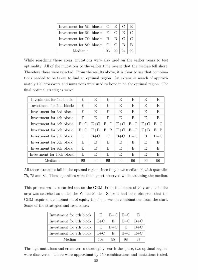
Investment for 5th block: C E C E

Investment for 6th block: E C E C

Investment for 7th block: B B C C

Investment for 8th block: C C B B

Median : 93 99 94 99

While searching these areas, mutations were also used on the earlier years to test

optimality. All of the mutations to the earlier time meant that the median fell short.

Therefore these were rejected. From the results above, it is clear to see that combina-

tions needed to be taken to find an optimal region. An extensive search of approxi-

mately 190 crossovers and mutations were used to hone in on the optimal region. The

final optimal strategies were:

Investment for 1st block: E E E E E E E

Investment for 2nd block: E E E E E E E

Investment for 3rd block: E E E E E E E

Investment for 4th block: E E E E E E E

Investment for 5th block: E+C E+C E+C E+C E+C E+C E+C

Investment for 6th block: E+C E+B E+B E+C E+C E+B E+B

Investment for 7th block: C B+C C B+C B+C B B+C

Investment for 8th block: E E E E E E E

Investment for 9th block: E E E E E E E

Investment for 10th block: E E E E E E E

Median : 96 96 96 96 96 96 96

All these strategies fall in the optimal region since they have median 96 with quantiles

75, 78 and 84. These quantiles were the highest observed while attaining the median.

This process was also carried out on the GBM. From the blocks of 20 years, a similar

area was searched as under the Wilkie Model. Since it had been observed that the

GBM required a combination of equity the focus was on combinations from the start.

Some of the strategies and results are:

Investment for 5th block: E E+C E+C E

Investment for 6th block: E+C E E+C B+C

Investment for 7th block: E B+C E B+C

Investment for 8th block: E+C E B+C E+C

Median : 108 98 98 97

Through mutations and crossover to thoroughly search the space, two optimal regions

were discovered. There were approximately 150 combinations and mutations tested.

58

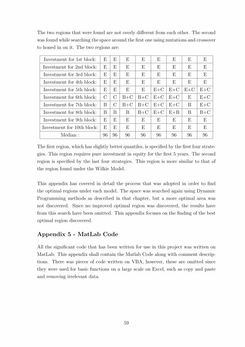
The two regions that were found are not overly different from each other. The second

was found while searching the space around the first one using mutations and crossover

to honed in on it. The two regions are:

Investment for 1st block: E E E E E E E E

Investment for 2nd block: E E E E E E E E

Investment for 3rd block: E E E E E E E E

Investment for 4th block: E E E E E E E E

Investment for 5th block: E E E E E+C E+C E+C E+C

Investment for 6th block: C C B+C B+C E+C E+C E E+C

Investment for 7th block: B C B+C B+C E+C E+C B E+C

Investment for 8th block: B B B B+C E+C E+B B B+C

Investment for 9th block: E E E E E E E E

Investment for 10th block: E E E E E E E E

Median : 96 96 96 96 96 96 96 96

The first region, which has slightly better quantiles, is specified by the first four strate-

gies. This region requires pure investment in equity for the first 5 years. The second

region is specified by the last four strategies. This region is more similar to that of

the region found under the Wilkie Model.

This appendix has covered in detail the process that was adopted in order to find

the optimal regions under each model. The space was searched again using Dynamic

Programming methods as described in that chapter, but a more optimal area was

not discovered. Since no improved optimal region was discovered, the results have

from this search have been omitted. This appendix focuses on the finding of the best

optimal region discovered.

Appendix 5 - MatLab Code

All the significant code that has been written for use in this project was written on

MatLab. This appendix shall contain the Matlab Code along with comment descrip-

tions. There was pieces of code written on VBA, however, these are omitted since

they were used for basic functions on a large scale on Excel, such as copy and paste

and removing irrelevant data.

59

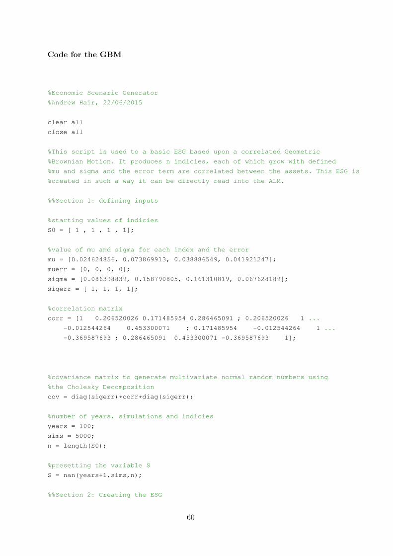
Code for the GBM

%Economic Scenario Generator

%Andrew Hair, 22/06/2015

clear all

close all

%This script is used to a basic ESG based upon a correlated Geometric

%Brownian Motion. It produces n indicies, each of which grow with defined

%mu and sigma and the error term are correlated between the assets. This ESG is

%created in such a way it can be directly read into the ALM.

%%Section 1: defining inputs

%starting values of indicies

S0 = [ 1 , 1 , 1 , 1];

%value of mu and sigma for each index and the error

mu = [0.024624856, 0.073869913, 0.038886549, 0.041921247];

muerr = [0, 0, 0, 0];

sigma = [0.086398839, 0.158790805, 0.161310819, 0.067628189];

sigerr = [ 1, 1, 1, 1];

%correlation matrix

corr = [1 0.206520026 0.171485954 0.286465091 ; 0.206520026 1 ...

-0.012544264 0.453300071 ; 0.171485954 -0.012544264 1 ...

-0.369587693 ; 0.286465091 0.453300071 -0.369587693 1];

%covariance matrix to generate multivariate normal random numbers using

%the Cholesky Decomposition

cov = diag(sigerr)*corr*diag(sigerr);

%number of years, simulations and indicies

years = 100;

sims = 5000;

n = length(S0);

%presetting the variable S

S = nan(years+1,sims,n);

%%Section 2: Creating the ESG

60

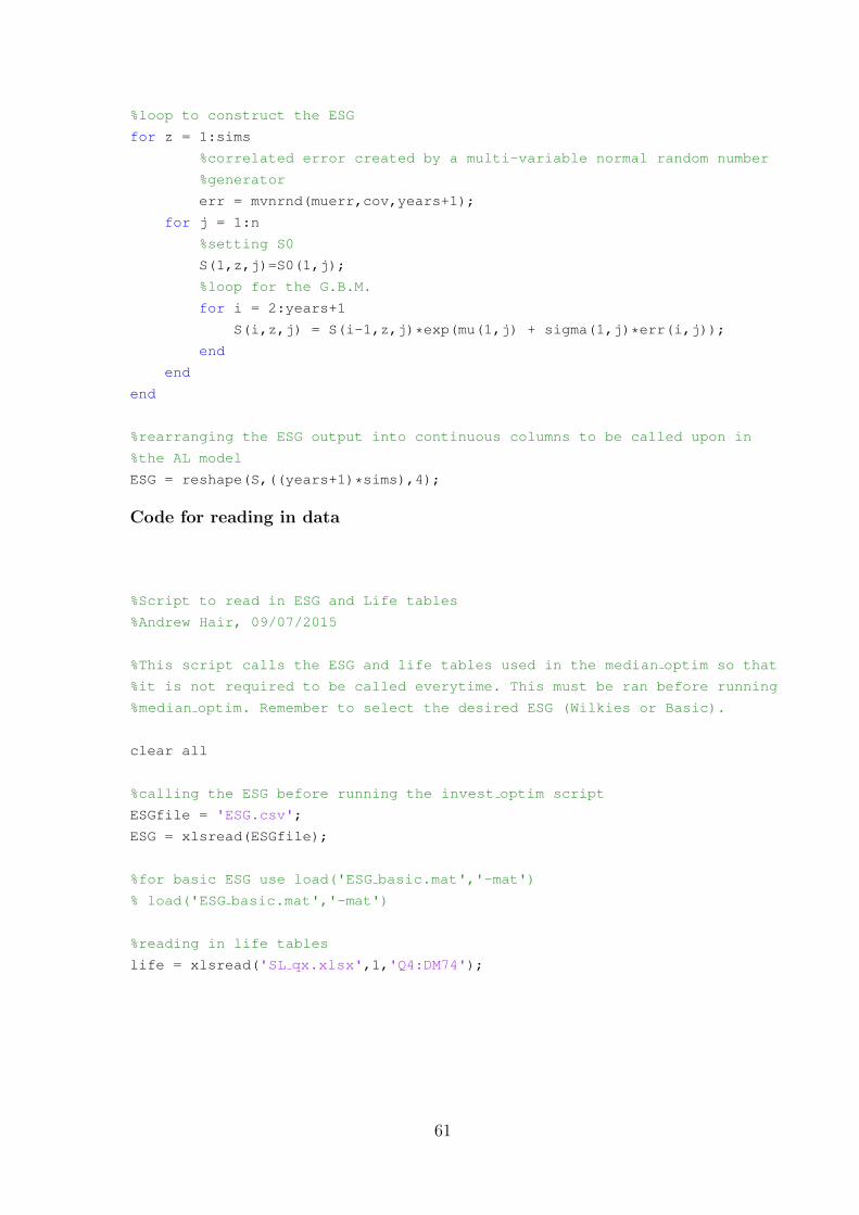
%loop to construct the ESG

for z = 1:sims

%correlated error created by a multi-variable normal random number

%generator

err = mvnrnd(muerr,cov,years+1);

for j = 1:n

%setting S0

S(1,z,j)=S0(1,j);

%loop for the G.B.M.

for i = 2:years+1

S(i,z,j) = S(i-1,z,j)*exp(mu(1,j) + sigma(1,j)*err(i,j));

end

end

end

%rearranging the ESG output into continuous columns to be called upon in

%the AL model

ESG = reshape(S,((years+1)*sims),4);

Code for reading in data

%Script to read in ESG and Life tables

%Andrew Hair, 09/07/2015

%This script calls the ESG and life tables used in the median optim so that

%it is not required to be called everytime. This must be ran before running

%median optim. Remember to select the desired ESG (Wilkies or Basic).

clear all

%calling the ESG before running the invest optim script

ESGfile = 'ESG.csv';

ESG = xlsread(ESGfile);

%for basic ESG use load('ESG basic.mat','-mat')

% load('ESG basic.mat','-mat')

%reading in life tables

life = xlsread('SL qx.xlsx',1,'Q4:DM74');

61

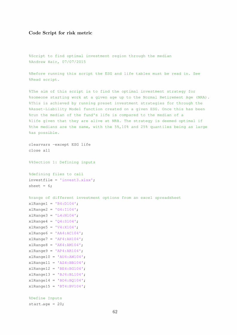
Code Script for risk metric

%Script to find optimal investment region through the median

%Andrew Hair, 07/07/2015

%Before running this script the ESG and life tables must be read in. See

%Read script.

%The aim of this script is to find the optimal investment strategy for

%someone starting work at a given age up to the Normal Retirement Age (NRA).

%This is achieved by running preset investment strategies for through the

%Asset-Liability Model function created on a given ESG. Once this has been

%run the median of the fund's life is compared to the median of a

%life given that they are alive at NRA. The strategy is deemed optimal if

%the medians are the same, with the 5%,10% and 25% quantiles being as large

%as possible.

clearvars -except ESG life

close all

%%Section 1: Defining inputs

%defining files to call

investfile = 'invest3.xlsx';

sheet = 6;

%range of different investment options from an excel spreadsheet

xlRange1 = 'B4:D104';

xlRange2 = 'G4:I104';

xlRange3 = 'L4:N104';

xlRange4 = 'Q4:S104';

xlRange5 = 'V4:X104';

xlRange6 = 'AA4:AC104';

xlRange7 = 'AF4:AH104';

xlRange8 = 'AK4:AM104';

xlRange9 = 'AP4:AR104';

xlRange10 = 'AU4:AW104';

xlRange11 = 'AZ4:BB104';

xlRange12 = 'BE4:BG104';

xlRange13 = 'BJ4:BL104';

xlRange14 = 'BO4:BQ104';

xlRange15 = 'BT4:BV104';

%Define Inputs

start age = 20;

62

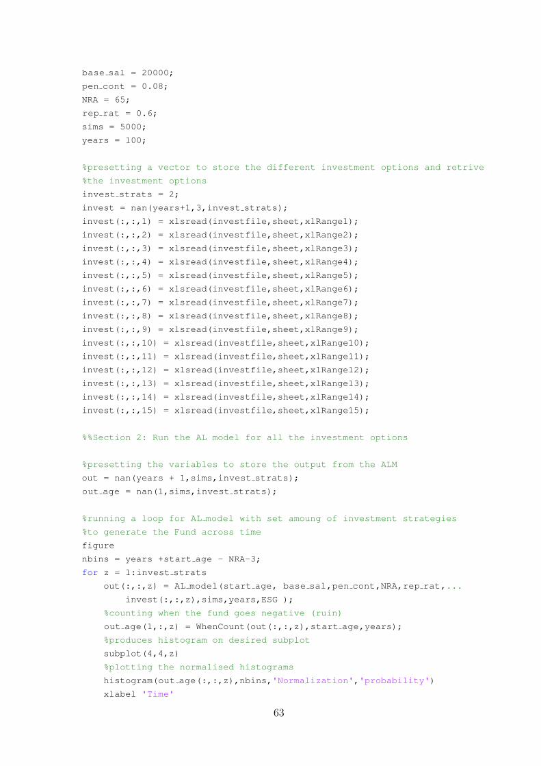
base sal = 20000;

pen cont = 0.08;

NRA = 65;

rep rat = 0.6;

sims = 5000;

years = 100;

%presetting a vector to store the different investment options and retrive

%the investment options

invest strats = 2;

invest = nan(years+1,3,invest strats);

invest(:,:,1) = xlsread(investfile,sheet,xlRange1);

invest(:,:,2) = xlsread(investfile,sheet,xlRange2);

invest(:,:,3) = xlsread(investfile,sheet,xlRange3);

invest(:,:,4) = xlsread(investfile,sheet,xlRange4);

invest(:,:,5) = xlsread(investfile,sheet,xlRange5);

invest(:,:,6) = xlsread(investfile,sheet,xlRange6);

invest(:,:,7) = xlsread(investfile,sheet,xlRange7);

invest(:,:,8) = xlsread(investfile,sheet,xlRange8);

invest(:,:,9) = xlsread(investfile,sheet,xlRange9);

invest(:,:,10) = xlsread(investfile,sheet,xlRange10);

invest(:,:,11) = xlsread(investfile,sheet,xlRange11);

invest(:,:,12) = xlsread(investfile,sheet,xlRange12);

invest(:,:,13) = xlsread(investfile,sheet,xlRange13);

invest(:,:,14) = xlsread(investfile,sheet,xlRange14);

invest(:,:,15) = xlsread(investfile,sheet,xlRange15);

%%Section 2: Run the AL model for all the investment options

%presetting the variables to store the output from the ALM

out = nan(years + 1,sims,invest strats);

out age = nan(1,sims,invest strats);

%running a loop for AL model with set amoung of investment strategies

%to generate the Fund across time

figure

nbins = years +start age - NRA-3;

for z = 1:invest strats

out(:,:,z) = AL model(start age, base sal,pen cont,NRA,rep rat,...

invest(:,:,z),sims,years,ESG );

%counting when the fund goes negative (ruin)

out age(1,:,z) = WhenCount(out(:,:,z),start age,years);

%produces histogram on desired subplot

subplot(4,4,z)

%plotting the normalised histograms

histogram(out age(:,:,z),nbins,'Normalization','probability')

xlabel 'Time'

63

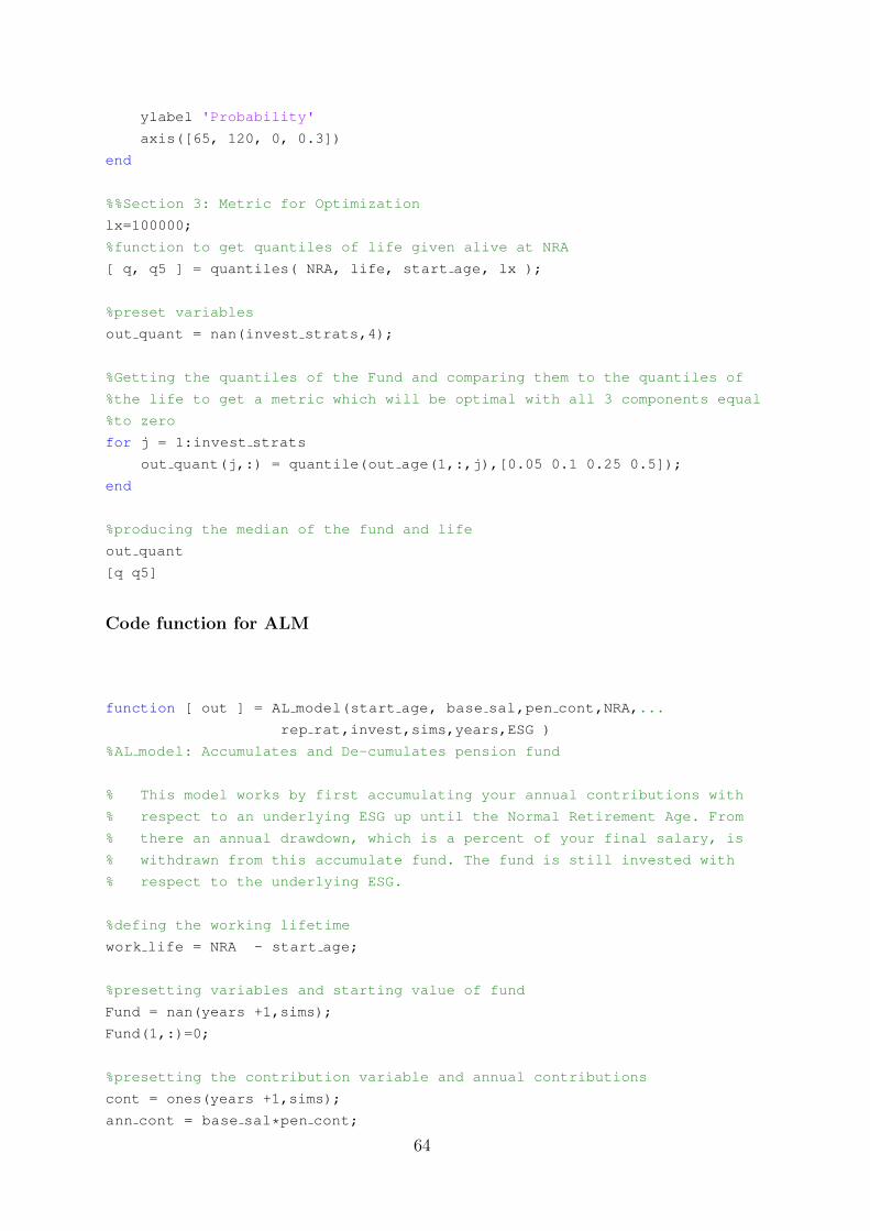
ylabel 'Probability'

axis([65, 120, 0, 0.3])

end

%%Section 3: Metric for Optimization

lx=100000;

%function to get quantiles of life given alive at NRA

[ q, q5 ] = quantiles( NRA, life, start age, lx );

%preset variables

out quant = nan(invest strats,4);

%Getting the quantiles of the Fund and comparing them to the quantiles of

%the life to get a metric which will be optimal with all 3 components equal

%to zero

for j = 1:invest strats

out quant(j,:) = quantile(out age(1,:,j),[0.05 0.1 0.25 0.5]);

end

%producing the median of the fund and life

out quant

[q q5]

Code function for ALM

function [ out ] = AL model(start age, base sal,pen cont,NRA,...

rep rat,invest,sims,years,ESG )

%AL model: Accumulates and De-cumulates pension fund

% This model works by first accumulating your annual contributions with

% respect to an underlying ESG up until the Normal Retirement Age. From

% there an annual drawdown, which is a percent of your final salary, is

% withdrawn from this accumulate fund. The fund is still invested with

% respect to the underlying ESG.

%defing the working lifetime

work life = NRA - start age;

%presetting variables and starting value of fund

Fund = nan(years +1,sims);

Fund(1,:)=0;

%presetting the contribution variable and annual contributions

cont = ones(years +1,sims);

ann cont = base sal*pen cont;

64

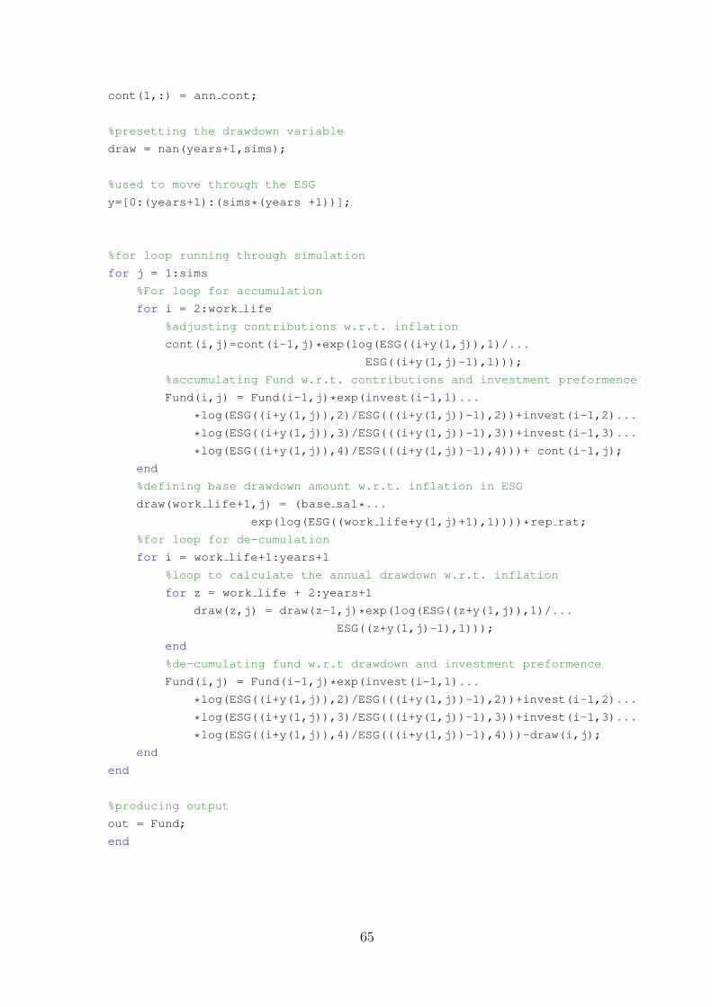
cont(1,:) = ann cont;

%presetting the drawdown variable

draw = nan(years+1,sims);

%used to move through the ESG

y=[0:(years+1):(sims*(years +1))];

%for loop running through simulation

for j = 1:sims

%For loop for accumulation

for i = 2:work life

%adjusting contributions w.r.t. inflation

cont(i,j)=cont(i-1,j)*exp(log(ESG((i+y(1,j)),1)/...

ESG((i+y(1,j)-1),1)));

%accumulating Fund w.r.t. contributions and investment preformence

Fund(i,j) = Fund(i-1,j)*exp(invest(i-1,1)...

*log(ESG((i+y(1,j)),2)/ESG(((i+y(1,j))-1),2))+invest(i-1,2)...

*log(ESG((i+y(1,j)),3)/ESG(((i+y(1,j))-1),3))+invest(i-1,3)...

*log(ESG((i+y(1,j)),4)/ESG(((i+y(1,j))-1),4)))+ cont(i-1,j);

end

%defining base drawdown amount w.r.t. inflation in ESG

draw(work life+1,j) = (base sal*...

exp(log(ESG((work life+y(1,j)+1),1))))*rep rat;

%for loop for de-cumulation

for i = work life+1:years+1

%loop to calculate the annual drawdown w.r.t. inflation

for z = work life + 2:years+1

draw(z,j) = draw(z-1,j)*exp(log(ESG((z+y(1,j)),1)/...

ESG((z+y(1,j)-1),1)));

end

%de-cumulating fund w.r.t drawdown and investment preformence

Fund(i,j) = Fund(i-1,j)*exp(invest(i-1,1)...

*log(ESG((i+y(1,j)),2)/ESG(((i+y(1,j))-1),2))+invest(i-1,2)...

*log(ESG((i+y(1,j)),3)/ESG(((i+y(1,j))-1),3))+invest(i-1,3)...

*log(ESG((i+y(1,j)),4)/ESG(((i+y(1,j))-1),4)))-draw(i,j);

end

end

%producing output

out = Fund;

end

65

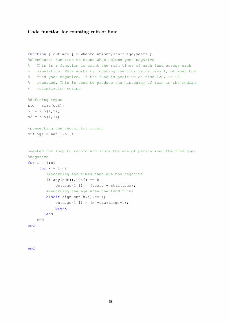
Code function for counting ruin of fund

function [ out age ] = WhenCount(out,start age,years )

%WhenCount: Function to count when column goes negative

% This is a function to count the ruin times of each fund across each

% simulation. This works by counting the tick value less 1, of when the

% fund goes negative. If the fund is positive at time 120, it is

% recorded. This is used to produce the histogram of ruin in the median

% optimization script.

%defining input

s o = size(out);

n1 = s o(1,2);

n2 = s o(1,1);

%presetting the vector for output

out age = nan(1,n1);

%nested for loop to record and store the age of person when the fund goes

%negative

for i = 1:n1

for x = 1:n2

%recording end times that are non-negative

if any(out(:,i)<0) == 0

out age(1,i) = (years + start age);

%recording the age when the fund ruins

elseif sign(out(x,i))==-1;

out age(1,i) = (x +start age-1);

break

end

end

end

end

66

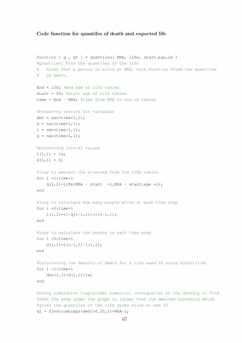
Code function for quantiles of death and expected life

function [ q , q5 ] = quantiles( NRA, life, start age,lx )

%Quantiles: Find the quantiles of the life

% Given that a person is alive at NRA, this function finds the quantiles

% of death.

End = 120; %end age of life tables

start = 50; %start age of life tables

time = End - NRA; %time from NRA to end of tables

%Presettng vectors for variables

den = nan(time+1,1);

d = nan(time+1,1);

l = nan(time+1,1);

q = nan(time+1,1);

%presetting initial values

l(1,1) = lx;

d(1,1) = 0;

%loop to extract the q-values from the life tables

for i =1:time+1

q(i,1)=life(NRA - start +i,NRA - start age +i);

end

%loop to calculate how many people alive at each time step

for i =2:time+1

l(i,1)=(1-q(i-1,1))*l(i-1,1);

end

%loop to calculate the deaths in each time step

for i =2:time+1

d(i,1)=l(i-1,1)-l(i,1);

end

%Calculating the density of death for a life aged 65 using d(x+n)/l(x)

for i =1:time+1

den(i,1)=d(i,1)/lx;

end

%Using cumulative trapazoidal numerical intergration on the density to find

%when the area under the graph is larger than the desired threshold which

%gives the quantiles of the life given alive at age 65

q1 = find(cumtrapz(den)>0.25,1)+NRA-1;

67

q2 = find(cumtrapz(den)>0.5,1)+NRA-1;

q3 = find(cumtrapz(den)>0.75,1)+NRA-1;

q5 = find(cumtrapz(den)>0.05,1)+NRA-1;

%output of the quantiles

q = [ q1 q2 q3];

q5;

end

68

Bibliography and References

[Ben, 1999] (1999). Dynamic programming.

http://web.csulb.edu/ obenli/Research/IE-encyc/dynprog.html. Accessed:

2015-08-20.

[jrf, 2008] (2008). A minimum income standard for britain.

http://www.jrf.org.uk/sites/files/jrf/2244.pdf. Accessed: 2015-08-19.

[lon, 2009] (2009). Longevitas.

http://www.longevitas.co.uk/site/informationmatrix/?tag=curve+of+deaths.

Accessed: 2015-08-19.

[ONS, 2013] (2013). Annual survey of hours and earnings uk, 2013.

http://www.ons.gov.uk/ons/rel/ashe/annual-survey-of-hours-and-earnings/2013-

provisional-results/info-ashe-2013.html. Accessed:

2015-08-19.

[HMT, 2014] (2014). Budget 2014: greater choive in pensions explained.

https://www.gov.uk/government/uploads/system/uploads/attachment data/file/301563/

Pensions fact sheet v8.pdf. Accessed: 2015-08-19.

[inv, 2015a] (2015a). Advanced Bond Concepts: bond pricing.

http://www.investopedia.com/university/advancedbond/advancedbond2.asp.

Accessed: 2015-08-19.

[cha, 2015] (2015). Challenger: protect your savings against sequencing risk.

http://www.challenger.com.au/retire/Sequencing.asp.

[fca, 2015] (2015). Financial Conduct Authority: income drawdown pensions.

http://www.fca.org.uk/firms/financial-services-products/investments/drawdown-

pensions.

[gov, 2015a] (2015a). gov.uk: personal and stakeholder penisons.

https://www.gov.uk/personal-pensions-your-rights/overview.

[hlw, 2015] (2015). Hargreaves Lansdown: how does it work?

http://www.hl.co.uk/pensions/drawdown/how-does-it-work.

69

[inv, 2015b] (2015b). Investment math.

http://thismatter.com/money/investments/investment-math.htm. Accessed:

2015-08-19.

[pas, 2015a] (2015a). Pension Advisory Service: automatic enrolment: How much

do i and my employer have to pay?

http://www.pensionsadvisoryservice.org.uk/about-pensions/pensions-

basics/automatic-enrolment/how-much-do-i-and-my-employer-have-to-pay.

[pas, 2015b] (2015b). Pension Advisory Service: new rules for income drawdown.

http://www.pensionsadvisoryservice.org.uk/news/new-rules-for-income-

drawdown. Accessed:

2015-08-18.

[gov, 2015b] (2015b). Retirement age. https://www.gov.uk/retirement-age.

Accessed: 2015-08-19.

[sea, 2015] (2015). Searching for an optimal solution.

http://users.ecs.soton.ac.uk/jn2/simulation/optimization.html. Accessed:

2015-08-20.

[Sto, 2015] (2015). Standard deviation volatility.

http://stockcharts.com/school/doku.php?id=chart school:technical indicators:

standard deviation volatility. Accessed: 2015-08-19.

[epi, 2015] (2015). Statistic and Research Methodology: comparing the mean and

the median.

https://epilab.ich.ucl.ac.uk/coursematerial/statistics/summarising centre spread/

measures centre/comparing mean median.html.

[Aris, 1964] Aris, R. (1964). Discrete Dynamic Programming: An Introduction.

Blaisdell.

[Bellman and Kalaba, 1965] Bellman, R. and Kalaba, R. E. (1965). Dynamic

programming and modern control theory. Academic Press New York.

[Bertsekas, 1995] Bertsekas, D. P. (1995). Dynamic programming and optimal

control, volume 1. Athena Scientific Belmont, MA.

[Blake et al., 2006] Blake, D., Cairns, A. J., and Dowd, K. (2006). Living with

mortality: Longevity bonds and other mortality-linked securities. British

Actuarial Journal, 12(01):153–197.

70

[Brigo et al., 2007] Brigo, D., Dalessandro, A., Neugebauer, M., and Triki, F. (2007).

A stochastic processes toolkit for risk management. Available at SSRN 1109160.

[Chang et al., 2011] Chang, C.-L., Jimenez-Martın, J.-A., McAleer, M., and

Perez Amaral, T. (2011). Risk management of risk under the basel accord:

Forecasting value-at-risk of vix futures. Available at SSRN 1765202.

[Ciecka and Ciecka, 1996] Ciecka, J. and Ciecka, P. (1996). Life expectancy and the

properties of survival data. Litigation Economics Digest, 1(2):19–33.

[Crouch et al., 2013] Crouch, K., Allen, G., Whitehead, F., Carter, A., and Levy, R.

(2013). Retirement choices: Baseline to measure effectiveness of the code of

conduct. Technical report, Association of British Insurers.

[Devaraj, 2013] Devaraj, D. (2013). Appendix 1: working principl of genetic

alogorithm.

http://shodhganga.inflibnet.ac.in/bitstream/10603/10246/11/11 appendices%201%20

to%203.pdf. Accessed: 2015-08-20.

[Dutta et al., 2000] Dutta, J., Kapur, S., and Orszag, J. M. (2000). A portfolio

approach to the optimal funding of pensions. Economics Letters, 69(2):201–206.

[Eiselt and Sandblom, 2012] Eiselt, H. A. and Sandblom, C.-L. (2012). Operations

research: a model-based approach. Springer Science & Business Media.

[Forrest, 1993] Forrest, S. (1993). Genetic algorithms: principles of natural selection

applied to computation. Science, 261(5123):872–878.

[Fraysse, 2015] Fraysse, H. (2015). The use of economic scenarios generators in

unstable economic periods. In SCOR Papers.

[Gerlach et al., 2012] Gerlach, R. H., Chen, C. W., and Chan, N. Y. (2012).

Bayesian time-varying quantile forecasting for value-at-risk in financial markets.

Journal of Business & Economic Statistics.

[Gerrard et al., 2004] Gerrard, R., Haberman, S., and Vigna, E. (2004). Optimal

investment choices post-retirement in a defined contribution pension scheme.

Insurance: Mathematics and Economics, 35(2):321–342.

[Glasserman, 2003] Glasserman, P. (2003). Monte Carlo methods in financial

engineering, volume 53. Springer Science & Business Media.

[Hibbert et al., 2001] Hibbert, J., Mowbray, P., and Turnbull, C. (2001). A

stochastic asset model & calibration for long-term financial planning purposes. In

Finance and Investment Conference.

71

[Horchler, 2011] Horchler, A. D. (2011). Stochastic Differential Equation toolbox:

For Use with MATLAB R2015a;

user′sGuide

. Andrew D. Horchler.

[Huber, 1995] Huber, P. (1995). A review of Wilkie’s stochastic investment model.

City Univ., Department of Actuarial Science and Statistics.

[Hull, 2015] Hull, I. (2015). Approximate dynamic programming with post-decision

states as a solution method for dynamic economic models. Journal of Economic

Dynamics and Control, 55:57–70.

[James, 2011] James, T. (2011). Approximate dynamic programming.

http://www.lancs.ac.uk/ jamest/content/ADP Terry.pdf.

[Joss, 2012] Joss, R. (2012). A fresh look at lognormal forecasting. Risk and

Reward, 59:16–18.

[Judd, 1998] Judd, K. L. (1998). Numerical methods in economics. MIT press.

[Lorena et al., 2002] Lorena, L. A., Narciso, M. G., and Beasley, J. (2002). A

constructive genetic algorithm for the generalized assignment problem.

Evolutionary Optimization, 5:1–19.

[Milevsky and Abaimova, 2006] Milevsky, M. and Abaimova, A. (2006). Retirement

income and the sensitive sequence of returns. Technical report, Metlife.

[Milevsky, 2007] Milevsky, M. A. (2007). A gentle introduction to the calculus of

sustainable income: What is your retirement risquotient? Journal of Financial

Service Professionals, 61(4):51.

[Mowbray, 2009] Mowbray, P. (2009). Investment strategy design for defined

contribution pension plans. Technical report, Moody’s Analytics.

[Revees and Rowe, 2004] Revees, C. and Rowe, J. (2004). Genetic

algorithms–principles and perspectives.

[Rosu, 2002] Rosu, I. (2002). The bellman principle of optimality. Availiable at:

http://faculty. chicagogsb. edu/ioanid. rosu/research/notes/bellman. pdf.

[Sahin et al., 2008] Sahin, S., Cairns, A., and Kleinow, T. (2008). Revisiting the

wilkie investment model. In The 18th AFIR Colloquium: Financial Risk in a

Changing World, Rome.

72

[Sgouropoulos et al., 2014] Sgouropoulos, N., Yao, Q., and Yastremiz, C. (2014).

Matching a distribution by matching quantiles estimation. Journal of the

American Statistical Association, (just-accepted):00–00.

[Sheppard, 2012] Sheppard, M. (2012). Fit all valid parametric probabilitiy

distributions to data: For Use with MATLAB R2015a. MatLab Central.

[Sheshinski, 2007] Sheshinski, E. (2007). The economic theory of annuities.

Economics Books, 1.

[Shirai, 2010] Shirai, K. (2010). Interest rate risk modeling using extended

lognormal distribution with variable volatility. Stochastic Modeling.

[Vernic et al., 2009] Vernic, R., Teodorescu, S., and Pelican, E. (2009). Two

lognormal models for real data. Annals of Ovidius University, Series

Mathematics, 17(3):263–277.

[Wadsworth et al., 2000] Wadsworth, M., Findlater, A., and Boardman, T. (2000).

Reinventing annuities. Watson Wyatt Partners.

[Wilkie and Sahin, 2015] Wilkie, A. and Sahin, S. (2015). Yet more on a stochastic

economic model: Part 2: Initial conidions, select periods and neutralising

parameters. Submitted.

[Wilkie et al., 2011] Wilkie, A., Sahin, S., Cairns, A., and Kleinow, T. (2011). Yet

more on a stochastic economic model: part 1: updating and refitting, 1995 to

2009. Annals of Actuarial Science, 5(01):53–99.

[Wilkie et al., 2003] Wilkie, A., Waters, H. R., and Yang, S. (2003). Reserving,

pricing and hedging for policies with guaranteed annuity options. British

Actuarial Journal, 9(02):263–391.

[Wilkie, 1984] Wilkie, A. D. (1984). A stochastic investment model for actuarial

use. Transactions of the Faculty of Actuaries, 39:341–403.

[Wilkie, 1995] Wilkie, A. D. (1995). More on a stochastic asset model for actuarial

use. British Actuarial Journal, 1(05):777–964.

73