
Anderson Travia INTERACTION CROSS SECTIONS NEEDED FOR SIMULATION
119
Transcript of Anderson Travia INTERACTION CROSS SECTIONS NEEDED FOR SIMULATION


Anderson Travia INTERACTION CROSS SECTIONS NEEDED FOR
SIMULATION OF SECONDARY ELECTRON EMISSION SPECTRA FROM THIN
METAL FOILS AFTER FAST PROTON IMPACT (Under the direction ofDr.
Michael Dingfelder) Department of Physics, June 2009
Monte Carlo simulations of secondary electron emission from thin metal foils after
fast proton impact require reliable interaction cross sections with the target under
consideration. Total and energy differential inelastic cross sections have been derived
for aluminum, copper, and gold thin-metal foils within the plane-wave first Born
approximation (PWFBA) that factorizes the double cross section into the generalized
oscillator strength and kinematic factors. The generalized oscillator strength or Bethe
surface of the medium is obtained by using a semi-empirical optical oscillator strength
distribution published in the literature and an extension algorithm based on the
delta-oscillator model. Energy differential, total, and stopping cross sections are then
obtained by simple integrations. Comparisons with other calculations and
experimental values from the literature show that our modeloffers a good agreement
in the energy range considered. As a final step, the cross sections and a transport
model for copper have been implemented into the Monte Carlo track structure code
PARTRAC where simulations of secondary electron emission spectra from copper foil
have been performed.

INTERACTION CROSS SECTIONS NEEDED FOR SIMULATION OF
SECONDARY ELECTRON EMISSION SPECTRA FROM THIN METAL FOILS
AFTER FAST PROTON IMPACT
A THESIS
PRESENTED TO
THE FACULTY OF THE DEPARTMENT OF PHYSICS
EAST CAROLINA UNIVERSITY
In Partial Fulfillment
of the Requirements for the Degree
Master of Science in Applied Physics
by
Anderson Travia
June, 2009
INTERACTION CROSS SECTIONS NEEDED FOR SIMULATION OF
SECONDARY ELECTRON EMISSION SPECTRA FROM THIN METAL FOILS
AFTER FAST PROTON IMPACT
by
Anderson Travia
APPROVED BY:
DIRECTOR OF THESIS:
____________________________________
Michael Dingfelder, Ph. D.
COMMITTEE MEMBER:
____________________________________
Larry H. Toburen, Ph. D.
COMMITTEE MEMBER:
____________________________________
Jefferson L. Shinpaugh, Ph. D.
COMMITTEE MEMBER:
____________________________________
David W. Pravica, Ph. D.
INTERIM CHAIR OF THE DEPARTMENT OF PHYSICS:
____________________________________
James M. Joyce, Ph. D.
DEAN OF GRADUATE SCHOOL:
_____________________________________
Paul J. Gemperline, Ph. D.

Acknowledgements
I would like to thank the Department of Physics of East Carolina University and in
special Dr. Michael Dingfelder and Dr. Larry H. Toburen for providing the means for
the conclusion of this project. Needless to say, without their generosity and assistance
the conclusion of this study would be just impossible. Thankyou very much for your
lectures, comments, suggestions, and supervision. I also would like to thank Dr.
Jefferson L. Shinpaugh and Dr. David W. Pravica for taking their time to read this
work and for providing their also extremely important criticism. Finally, I would like
to thank my wife for supporting me through this tough journey.
Table of Contents
List of Figures . . . . . . . . . . . . . . . . . . . . . . . . . . . . . . . . . . . . . .. . . . . . . . . . . .vii
1 Introduction 1
1.1 Initial facts and observations . . . . . . . . . . . . . . . . . . . . .. . . . . . . . . . . . . 1
1.2 Motivation and objectives . . . . . . . . . . . . . . . . . . . . . . . . .. . . . . . . . . . . 2
2 Theory 5
2.1 Basic principles . . . . . . . . . . . . . . . . . . . . . . . . . . . . . . . . .. . . . . . . . . . 5
2.1.1 Cross-sections . . . . . . . . . . . . . . . . . . . . . . . . . . . . . . . .. . . . . . . . 5
2.1.2 From Maxwell’s equations to differential cross-sections . . . . . . . . . . 8
2.2 The electric field due to an induced charged density . . . . .. . . . . . . . . . . . .11
2.3 Modeling the current charge density . . . . . . . . . . . . . . . . .. . . . . . . . . . . .15
2.3.1 The point radiator . . . . . . . . . . . . . . . . . . . . . . . . . . . . . .. . . . . . .15
2.3.2 Scattering power for the oscillating free electron . .. . . . . . . . . . . . .16
2.3.3 The scattering cross-section of a single free electron . . . . . . . . . . . . 19
2.3.4 Scattering by bound electrons . . . . . . . . . . . . . . . . . . . .. . . . . . . . 22
2.3.5 Scattering by many-electron atoms . . . . . . . . . . . . . . . .. . . . . . . . 24
2.4 The atomic scattering factor and the oscillator strength . . . . . . . . . . . . . . . 27
2.5 Bethe theory and the GOS of a material . . . . . . . . . . . . . . . . .. . . . . . . . . 30
2.6 GOS Hartree-Fock approximation for single atomic collision . . . . . . . . . . 32
2.7 DICS in condensed-phase - modeling the energy-loss function . . . . . . . . . 35
2.7.1 The key quantity - energy-loss function . . . . . . . . . . . .. . . . . . . . . .35
2.7.2 Link with the differential cross section and GOS . . . . .. . . . . . . . . 37
2.8 Monte Carlo simulation of radiation transport . . . . . . . .. . . . . . . . . . . . . .39
2.8.1 Tracking of a charged particle . . . . . . . . . . . . . . . . . . . .. . . . . . . . 39
2.8.2 The probability distribution function and sampling methods . . . . . . 40
2.8.3 Random track generation . . . . . . . . . . . . . . . . . . . . . . . . .. . . . . . .42
2.8.4 An example using a hypothetical mean-free-path PDF . .. . . . . . . . .43
3 Procedures 45
3.1 Consistency test for the OOS - sum-rule test . . . . . . . . . . .. . . . . . . . . . . .45
3.1.1 Aluminum OOS . . . . . . . . . . . . . . . . . . . . . . . . . . . . . . . . . . .. . . 48
3.1.2 Copper OOS . . . . . . . . . . . . . . . . . . . . . . . . . . . . . . . . . . . . .. . . .49
3.1.3 Gold OOS . . . . . . . . . . . . . . . . . . . . . . . . . . . . . . . . . . . . . . .. . . 50
3.2 Limits of integration . . . . . . . . . . . . . . . . . . . . . . . . . . . . .. . . . . . . . . . .51
3.3 Shell separation . . . . . . . . . . . . . . . . . . . . . . . . . . . . . . . . .. . . . . . . . . . 57
3.3.1 Aluminum edge-energies . . . . . . . . . . . . . . . . . . . . . . . . .. . . . . . .58
3.3.2 Copper edge-energies . . . . . . . . . . . . . . . . . . . . . . . . . . .. . . . . . . 58
3.3.3 Gold edge-energies . . . . . . . . . . . .. . . . . . . . . . . . . . . . .. . . . . . . .58
3.4 Angular distribution of primary and secondary particles . . . . . . . . . . . . . . .66
3.4.1 Angular distribution of primary protons. . . . . . . . . . .. . . . . . . . . . . 66
3.4.2 Angular distribution of primary electrons . . . . . . . . .. . . . . . . . . . . 68
3.4.3 Angular distribution of electrons induced by electron impact . . . . . . 69
3.4.4 Angular distribution of electrons induced by proton impact . . . . . . . 70
3.4.5 Determination of A(w) and B(w) . . . . . . . . . . . . . . . . . . . .. . . . . . .70
3.4.6 Aluminum, copper, and gold Bethe coefficients . . . . . . .. . . . . . . . . 73
4 Results 79
4.1 Electron impact in aluminum, copper, and gold thin foils. . . . . . . . . . . . . .80
4.1.1 Aluminum DIMFP, IMFP, and STP . . . . . . . . . . . . . . . . . . . . .. . . 80
4.1.2 Copper DIMFP, IMFP, and STP . . . . . . . . . . . . . . . . . . . . . . .. . . . 83
4.1.3 Gold DIMFP, IMFP, and STP . . . . . . . . . . . . . . . . . . . . . . . . .. . . .86
4.2 Proton impact in aluminum, copper, and gold thin foils . .. . . . . . . . . . . . . 89
4.2.1 Aluminum DIMFP, IMFP, and mass STP . . . . . . . . . . . . . . . . .. . . .89
4.2.2 Copper DIMFP, IMFP, and mass STP . . . . . . . . . . . . . . . . . . .. . . .92
4.2.3 Gold DIMFP, IMFP, and mass STP . . . . . . . . . . . . . . . . . . . . .. . . .95
4.3 Electron yields from 0.1 micron copper foil after 6 MeV proton impact . . . .98

4.3.1 Forward electron yield . . . . . . . . . . . . . . . . . . . . . . . . . .. . . . . . . 98
4.3.2 Backward electron yield . . . . . . . . . . . . . . . . . . . . . . . . .. . . . . . . 99
5 Conclusion and Remarks . . . . . . . . . . . . . . . . . . . . . . . . . . . . . .. . . . . . . . . 100
References . . . . . . . . . . . . . . . . . . . . . . . . . . . . . . . . . . . . . . . . .. . . . . . . . . . 102
List of Figures
1 Diagram for the scattering of an incident flux of particlesJin . . . . . . . . . . . . . . . .7
2 Coordinate system in the direction of the propagation of the incident wavek0 . . .14
3 sin2 θ radiation pattern of a small accelerated charge . . . . . . . . . .. . . . . . . . . . 19
4 Many-electron atom in three random electronic spatial configurations . . . . . . . .28
5 Graphical representation of the mean-free-path from a hypothetical PDF . . . . . . 44
6 Analysis of the integration routine used for integration of the OOS . . . . . . . . . . 47
7 Optical oscillator strength density distribution of aluminum. . . . . . . . . . . . . . . 48
8 Optical oscillator strength density distribution of copper . . . . . . . . . . . . . . . . . 49
9 Optical oscillator strength density distribution of gold. . . . . . . . . . . . . . . . . . . 50
10 Limits of integration for electron energy of 10 eV . . . . . . .. . . . . . . . . . . . . . . 52
11 Limits of integration for electron energy of 10 keV. . . . . .. . . . . . . . . . . . . . . .53
12 Limits of integration for proton energy of 100 eV. . . . . . . .. . . . . . . . . . . . . . .54
13 Limits of integration for proton energy of 10 MeV . . . . . . . .. . . . . . . . . . . . . .55
14 Aluminum OOS K, L, and M shell separation . . . . . . . . . . . . . . .. . . . . . . . . .59
15 Copper OOS K, L, and MN shell separation. . . . . . . . . . . . . . . .. . . . . . . . . . 60
16 Gold OOS K, L, M, N, O, and P shell separation. . . . . . . . . . . . .. . . . . . . . . . 61
17 Aluminum shell coefficients . . . . . . . . . . . . . . . . . . . . . . . . .. . . . . . . . . . . . 63
18 Copper shell coefficients . . . . . . . . . . . . . . . . . . . . . . . . . . .. . . . . . . . . . . . 64
19 Gold shell coefficients. . . . . . . . . . . . . . . . . . . . . . . . . . . . .. . . . . . . . . . . . .65
20 Classical scattering kinematics . . . . . . . . . . . . . . . . . . . .. . . . . . . . . . . . . . . 69
21 Bethe A coefficient, as defined in equation 114, for aluminum. . . . . . . . . . . . . 73
22 Bethe B coefficient, as defined in equation 115, for aluminum . . . . . . . . . . . . . 74
23 Bethe A coefficient, as defined by equation 114, for copper .. . . . . . . . . . . . . . 75
24 Bethe B coefficient, as defined by equation 115, for copper .. . . . . . . . . . . . . . 76
25 Bethe A coefficient, as defined by equation 114, for gold. . .. . . . . . . . . . . . . . 77
26 Bethe B coefficient, as defined in equation 115, for gold . . .. . . . . . . . . . . . . .78
27 DIMFP of electrons in aluminum. . . . . . . . . . . . . . . . . . . . . . .. . . . . . . . . . . 80
28 IMFP of electrons in aluminum . . . . . . . . . . . . . . . . . . . . . . . .. . . . . . . . . . .81
29 STP of aluminum for electron source. . . . . . . . . . . . . . . . . . .. . . . . . . . . . . . 82
30 DIMFP of electrons in copper. . . . . . . . . . . . . . . . . . . . . . . . .. . . . . . . . . . . .83
31 IMFP of electrons in copper . . . . . . . . . . . . . . . . . . . . . . . . . .. . . . . . . . . . . 84
32 STP of copper for electron source . . . . . . . . . . . . . . . . . . . . .. . . . . . . . . . . . 85
33 DIMFP of electrons in gold . . . . . . . . . . . . . . . . . . . . . . . . . . .. . . . . . . . . . .86
34 IMFP of electrons in gold . . . . . . . . . . . . . . . . . . . . . . . . . . . .. . . . . . . . . . . 87
35 STP of gold for electron source . . . . . . . . . . . . . . . . . . . . . . .. . . . . . . . . . . .88
36 DIMFP of protons in aluminum. . . . . . . . . . . . . . . . . . . . . . . . .. . . . . . . . . . 89

37 IMFP of protons in aluminum . . . . . . . . . . . . . . . . . . . . . . . . . .. . . . . . . . . . 90
38 Mass STP of aluminum for proton source . . . . . . . . . . . . . . . . .. . . . . . . . . . .91
39 DIMFP of protons in copper . . . . . . . . . . . . . . . . . . . . . . . . . . .. . . . . . . . . .92
40 IMFP of protons in copper. . . . . . . . . . . . . . . . . . . . . . . . . . . .. . . . . . . . . . .93
41 Mass STP of copper for proton source. . . . . . . . . . . . . . . . . . .. . . . . . . . . . . .94
42 DIMFP of protons in gold. . . . . . . . . . . . . . . . . . . . . . . . . . . . .. . . . . . . . . . 95
43 IMFP of protons in gold. . . . . . . . . . . . . . . . . . . . . . . . . . . . . .. . . . . . . . . . .96
44 Mass STP of gold for proton source. . . . . . . . . . . . . . . . . . . . .. . . . . . . . . . .97
45 MC simulation of forward electron yields from copper foil. . . . . . . . . . . . . . . 98
46 MC simulation of backward electron yields from copper foil . . . . . . . . . . . . . .99

1 Introduction
1.1 Initial facts and observations
The study of ionizing radiation is considered by many to begin with the work of the
German physicist Wilhelm Conrad Röntgen and the discovery of X- rays in 1895
[1, 2]. Although the effects of X- rays on materials were not initially well understood,
shortly after the announcement of its discovery, they were recognized as an important
tool for medical diagnosis, but unfortunately for many patients, X-rays were widely
adopted without a previous systematic and serious study of its dose-effect properties.
It later became evident that X-rays could severely damage biological tissue and
demanded a serious analysis not only of its possible applications but also of its
ionization effects.
To understand a phenomenon such as ionizing radiation is to have the ability to
completely describe its properties in particular, for obvious reasons, its effects on
biological medium, for example, water and hydrocarbons. More generally, it includes
the reliable capacity to accurately generate, measure, andpredict its effects in all
relevant systems. For the last 75 years, this has been an ongoing joined effort that
includes scientific work specially in physics, chemistry, and biology that are
developing the necessary theories and techniques while studying systems from full
bodies of experimental animals to base deoxyribonucleic acid (DNA) sequences in
target cells. Progressing from full organisms down to tissue, to cell, to chromosome,
and to the gene, finally, the diverse biological effects of ionizing radiation can all
ultimately be interpreted, understood, and explained in terms of disruptions in these
building blocks or base sequences [3, 4].

2
1.2 Motivation and objectives
This particular study is part of a research project initiated a few years ago at East
Carolina University, with two main purposes: To study the transport of secondary
electrons in condensed phase and its spectra distribution when emitted from the targets
and also to provide rigorous tests for Monte Carlo-based charged particle track
structure models used in radiobiology.
The tests began with preliminary comparisons between experimental results of doubly
differential electron-yields using two distinct experimental techniques (time of flight
and electrostatic) for hydrocarbon targets (electron-yields at 45 degrees from CH4,
C2H6, and C3H8) and the simulation results from the event-by-event charged particle
track structure Monte Carlo (MC) code PARTRAC using its semi-empirical cross
section models for liquid water. The main purpose was to testthe simulation at the
fundamental physics level or before any reactions take place. Since discrepancies were
observed between the results obtained from experiment and PARTRAC at the low and
high energy ranges (< 50 eV and> 1 keV) and could not be completely clarified from
this preliminary test on hydrocarbon foils using the water-cross sections available in
PARTRAC, the project was extended to provide experimental data for amorphous solid
water (ASW) and other important biological tissues. Exploration of the results from
ASW are currently been done and the experimental data obtained for metals are very
consistent and will provide an excellent testing ground [5].
Therefore, to make this starting test possible, new cross-sections representative of the
metals, which are used as substrate in the experiment, needed to be calculated and
implemented into PARTRAC using the similar plane-wave Borntheory as it was
previously done for water cross-sections used in PARTRAC. It is to fulfill this initial
step that I began the study of the interaction of fast chargedparticles in
condensed-phase media to obtain the necessary background to calculate these

3
cross-sections for aluminum, copper, and gold. This work requires the
accomplishment of the following main steps:
• Collect and study key resources in classical electrodynamics and dielectric
theory
• Study the plane wave first Born approximation (PWFBA) for description of
sources or projectiles
• Understand the oscillator strength concept for the analytical representation of the
targets
• Research and construct the optical oscillator strength (OOS) of the relevant
target materials
• Research a simple dispersion algorithm for the construction of the generalized
oscillator strength (GOS)
• Compare between the classical electrodynamics collision picture and the full
quantum mechanical treatment
• Search for key quantities and expressions that are relevantfor the determination
of the desired differential inelastic cross sections (DICS)
• develop and optimize numerical procedures for the calculation of DICS, total
cross sections (TCS), and consistency tests
• Format and graphically represent the obtained DICS and TCS calculations and
compare them with well known results

4
It is hoped that this study in association with others that are currently being performed
can help the group answer the questions that were set since the first data on carbon
foils. For instance, it is desired to understand the phenomenon of metal and water
foil-charging and its relation with the reduction of low energy electron-yields based on
the physical properties of the foils [5].

2 Theory
2.1 Basic principles
2.1.1 Cross-sections
An incident charged particle interacts with another by exerting a Coulomb force on it
that depends simultaneously on the charge of both particlesand the distance of
separation between them [6, 7]. Unfortunatelly, the study of the atomic structure and
properties of materials usually involves the simultaneousinteraction of a large amount
of charged particles, which is known as a many body problem that is impossible to be
precisely solved. Therefore, statistical tools must be employed when dealing with such
problems, and if statistical fluctuations can be minimized by taking a large number of
measurements, the searched properties and values can be inferred as an average over
them. It is from this necessity that the concept of cross section comes to play a
fundamental role in atomic physics.
Without being concerned with the precise way in which an incident particle interacts
simultaneously with a large number of target particles, possibly exchanging energy
and momentum with all of them, the desired properties are inferred by setting the
measurement devices to only “count” or detect the particlesthat satisfy a pre-defined
physical property. In an extremelly simplified way, this is experimentally done by
setting the detector’s position with respect to the incident particle’s direction, adjusting
the detector’s sensitivity, or measuring the scattering particle’s time-of-flight if the
scattered particle’s momentum and energy are desired. Fromthe following picture, see
figure 1, the analytical representation of the cross sectionfor a particular event can be
constructed as:
6
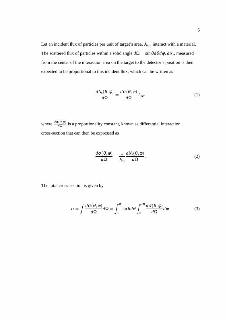
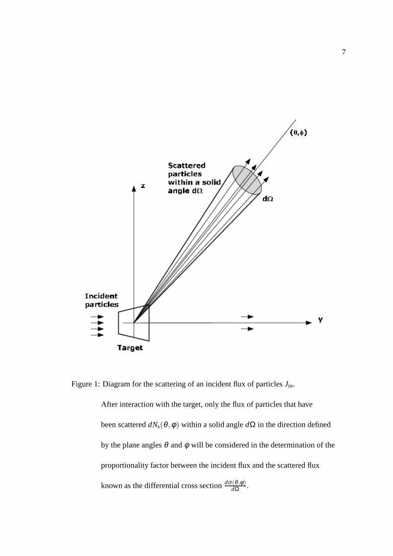
Let an incident flux of particles per unit of target’s area,Jinc, interact with a material.
The scattered flux of particles within a solid angledΩ = sinθdθdφ , dNs, measured
from the center of the interaction area on the target to the detector’s position is then
expected to be proportional to this incident flux, which can be written as
dNs(θ ,φ)
dΩ=
dσ(θ ,φ)
dΩJinc, (1)
wheredσ(θ ,φ)dΩ is a proportionality constant, known as differential interaction
cross-section that can then be expressed as
dσ(θ ,φ)
dΩ=
1Jinc
dNs(θ ,φ)
dΩ. (2)
The total cross-section is given by
σ =
ˆ
dσ(θ ,φ)
dΩdΩ =
ˆ π
0sinθdθ
ˆ 2π
0
dσ(θ ,φ)
dΩdφ . (3)
7
Figure 1: Diagram for the scattering of an incident flux of particlesJin.
After interaction with the target, only the flux of particlesthat have
been scattereddNs(θ ,φ) within a solid angledΩ in the direction defined
by the plane anglesθ andφ will be considered in the determination of the
proportionality factor between the incident flux and the scattered flux
known as the differential cross sectiondσ(θ ,φ)dΩ .

8
2.1.2 From Maxwell’s equations to differential cross-sections
The above over-simplified pictorial description of the experimental determination of a
differential cross-section can theoretically be more completely described from
ab-initio classical electrodynamics that obviously starts from the well known four
fundamental Maxwell’s equations [6, 7, 8, 9]
In the following equations, let∇ =−→∇ , E =
−→E (−→r , t), D =
−→D (−→r , t), B =
−→B (−→r , t),
H =−→H (−→r , t), A =
−→A (−→r , t), J =
−→J (−→r , t), andρ = ρ(−→r , t).
∇×H =∂D∂ t
+ J, (4)
∇×E = −∂B∂ t
, (5)
∇ ·B = 0, (6)
and
∇ ·D = ρ, (7)
where the electrical displacement and induced magnetic field are respectively defined
as
D = ε0E (8)
and
9
B = µ0H. (9)
To study the interaction of an incident electromagnetic field due, for example, to an
incident charged particle approaching the target with defined energy and momentum,
we need to obtain the wave equation that describes the movingfield. Recognizing the
vector identity
∇× (∇×A) = ∇(∇ ·A)−∇2A, (10)
the wave equation is obtained after following some basic steps, which start by taking
the curl of the Faraday’s Law. Following, is the complete derivation.
∇× (∇×E) = ∇×(−∂B
∂ t
)
∇(∇ ·E)−∇2E = −µ0∂∂ t
(∇×H)
−→∇(
ρε0
)−−→∇ 2
E = −µ0∂∂ t
(∂−→D∂ t
+−→J
)
∇(
ρε0
)−∇2E − ε0µ0
∂∂ t
(∂E∂ t
+Jε0
)
10
ε0µ0∂ 2E∂ t2 −∇2E = −µ0
∂J∂ t
− 1ε0
−→∇ ρ
(∂ 2
∂ t2 − c2∇2)
E = − 1ε0
[∂J∂ t
+ c2∇ρ]
Note that
c ≡ 1√ε0µ0
is the phase velocity of the moving radiation in vacuum, which is often referred as the
speed of “light in vacuum” withε0 andµ0 being the electric permitivity and magnetic
permeability of free space.
This wave equation is then the point of departure for explaining all the properties of
interest involving, for example, propagation, reflection,refraction, and in special for
this study the scattering processes with single and many-electron atoms involving free
and bound electrons.
Looking back into the wave-equation, we can interpret it as an association between
induced source terms on the right of the equation, given by the current and charge
densities, and the field they generate. Therefore, by appropriately representing the
response of the target to an incident electric field through the current and charge
densities induced in the material, the new field resulting from the induction process
can be in principle calculated.
The objective is then to solve the wave equation for the radiated electric fieldE(r, t) in
the presence of accelerated source terms represented by free or bound electrons and

11
combine this field with the incident polarization agent or inductive field to obtain the
resulting scattering wave.
2.2 The electric field due to an induced current charge density
To solve the wave equation
(∂ 2
∂ t2 − c2∇2)
E = − 1ε0
[∂J∂ t
+ c2∇ρ]
(11)
for E(r, t), in the presence of source terms, we can treat the quantity between
parentheses on the left of equation 11 as an operator and consider solving forE(r, t)
for arbitrary sources with the form
E(r, t) =
ˆ
[G(r, t)] [source]dr, (12)
whereG(r, t) represents the Green’s or response function due to the source term
[10, 11]. This can be considerably simplified if we move to thetemporalω and spatial
k frequency domains that are connected to the coordinater space through the
Fourier-Laplace transforms
E(−→r , t) =
ˆ
k
ˆ
ωEkωe−i(ωt−
−→k ·−→r ) dωdk
(2π)4 (13)
and

12
Ekω =
ˆ
r
ˆ
tE(−→r , t)ei(ωt−
−→k ·−→r )drdt, (14)
wheredω anddk correspond to scalar volume elements,Ekω = E(k,ω), and
ω = ωr + iωi, with ωi > 0. This is necessary for the convergence of equation 14 when
t → ∞.
Thus, in Laplace-Fourier space, the wave equation in operator form simplifies to
(ω2− k2c2)Ekω =1ε0
[(−iω)Jkω + ic2kρkω
], (15)
which can be solved for the electric field.
The path is clear now. If we construct appropriate models forthe sourcesJ(r, t) and
ρ(r, t), we can obtain the electric field from equation 15.
Using the equation for charge conservation
∇ · J +∂ρ∂ t
= 0, (16)
which is derived by taking the divergence of Ampere’s Law andthe known vector
relation∇ · (∇×A) = 0, the charge density can be written as
ρkω =
−→k · Jkω
ω. (17)
13
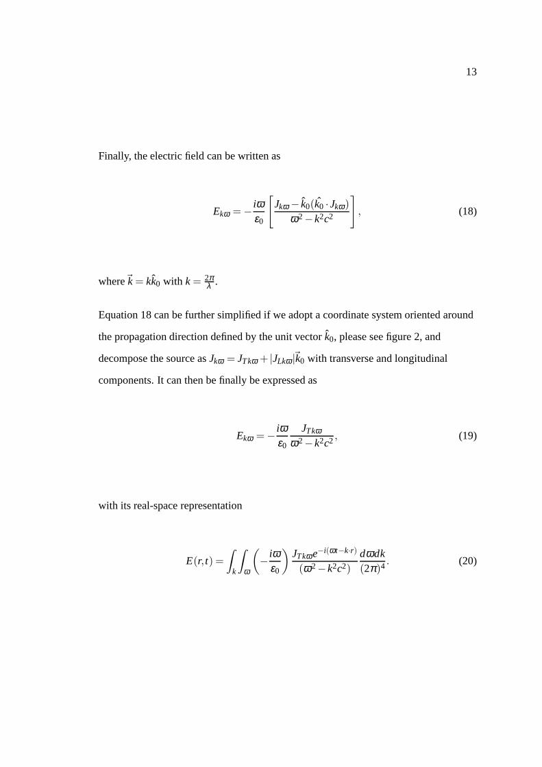
Finally, the electric field can be written as
Ekω = − iωε0
[Jkω − k0(k0 · Jkω)
ω2− k2c2
], (18)
where~k = kk0 with k = 2πλ .
Equation 18 can be further simplified if we adopt a coordinatesystem oriented around
the propagation direction defined by the unit vectork0, please see figure 2, and
decompose the source asJkω = JT kω + |JLkω |~k0 with transverse and longitudinal
components. It can then be finally be expressed as
Ekω = − iωε0
JTkωω2− k2c2 , (19)
with its real-space representation
E(r, t) =
ˆ
k
ˆ
ω
(− iω
ε0
)JTkωe−i(ωt−k·r)
(ω2− k2c2)
dωdk(2π)4 . (20)

14
Figure 2: Coordinate system in the direction of the propagation of the incident
wavek0. This simplifies the expression describing the radiation
field Ekω through the decomposition ofJkw into longitudinal
JLkw and transverseJT kw components.

15
2.3 Modeling the current charge density
2.3.1 The point radiator
Lets initially consider the case of an accelerating free electron that is small when
compared with the wavelength of the radiating field, thus allowing us to represent its
charge density by a Dirac delta function [6, 7, 8]. Thus, the moving electron can be
expressed as a current density given by
J = qn(r, t)−→v (r, t), (21)
whereq is the charge,n represents the particle number density, and−→v the particle’s
velocity.
The real-space and Laplace-Fourier space current densities are repectively
J = −eδ (r)−→v (t),
where in Cartesian coordinatesδ (r) = δ (x)δ (y)δ (z),
and
Jkω = −e−→v (ω), (22)
with transverse component
16
JT kω = −e−→v T (ω). (23)
Substituting this current density back into equation 20 andintegrating we can
recognize the expected connection between the radiated field and the particle’s
acceleration given by
E =e
4πε0c2rd−→v T (t − r/c)
dt(24)
and
E =e−→a T (t − r/c)
4πε0c2r. (25)
2.3.2 Scattering power for the oscillating free electron
The Poynting vector (energy flow or power per unit area) in electromagnetic theory is
given by [6, 7]
−→S (−→r , t) = E ×H. (26)
Again from Faraday’s Law and the definition of magnetic induction we can derive the
Magnetic fieldH as follows

17
∇×E = −∂B∂ t
B = µ0H
∇×E = −µ0∂H∂ t
ik×Ekω = iωµ0Hkω ,
from which we obtain
Hkω =
√ε0
µ0k0×Ekω , (27)
whereω = kc,with c = 1√ε0µ0for propagation in free space.
Using the vector identityA× (B×C) = (A ·C)B− (A ·B)C and the fact that for
transverse wavesk0 ·E = 0, we obtain
−→S (−→r , t) =
1Z0
|E|2k0, (28)
18
whereZ0 =√
µ0ε0
is the impedance of free space.
Noting thataT = |−→a T | = |−→a| sinθ the radiated power−→S (−→r , t) can be represented by
the acceleration, which reveals the familiar form for the dipole radiation [6, 7], see
figure 3 below.
−→S (−→r , t) =
e2|−→a |2sin2θ16π2ε0c3r2 k0 (29)
or
dPdΩ
=e2|−→a |2sin2 θ
16π2ε0c3 , (30)
where−→S (−→r , t) = dP
dA k0, for dA = r2dΩ.
The total power radiated immediately follows from the integration of equation 30,
P =8π3
(e2|−→a |2
16π2ε0c3
). (31)
Note that the average radiated power, which is used in the calculation of the
differential cross section for the radiation of an accelerated charged electron in the
direction defined by the acceleration vector−→a (−→r , t) can be expressed as [6, 7]
−→S =
12
Re[E ×H∗] (32)
19
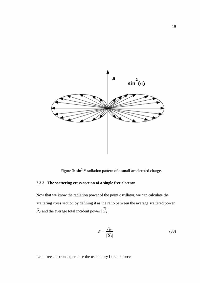
Figure 3: sin2θ radiation pattern of a small accelerated charge.
2.3.3 The scattering cross-section of a single free electron
Now that we know the radiation power of the point oscillator,we can calculate the
scattering cross section by defining it as the ratio between the average scattered power
Psc and the average total incident power|−→S i|,
σ =Psc
|−→S i|. (33)
Let a free electron experience the oscillatory Lorentz force
20
−→F = −e [Ei +
−→v ×Bi] , (34)
when in the presence of an incident field
Ei(r, t) = E0e−i(ωt−−→k ·−→r ). (35)
The equation of motion is then given by
m−→a = −e [Ei +−→v ×Bi] . (36)
The magnetic induction in this case is expressed as
Bi(r, t) =k0×Ei(
−→r , t)c
. (37)
Thus, we can neglect the−→v ×Bi, in equation 36 since it is proportional tov/c, which
is very small for non-relativistic velocities and equation36 simplifies to
−→a (−→r , t) = − em
Ei(−→r , t). (38)

21
The transverse component is obviously obtained by
aT = asinθ = − em|Ei|sinθ . (39)
Introducing the electron radiusre = e2
4πε0mc2 , the scattered electric field in the direction
θ with respect to the polarization direction of the incident field,
E(−→r , t) = −e2|Ei|sinθ4πε0mc2r
e−iω(t−r/c), (40)
can be more compactly written as
E(−→r , t) = −re|Ei|sinθr
e−iω(t−r/c). (41)
Therefore, the single free-electron scattering cross section (Thomson) can be written as
σ =Psc
|Si|=
4π3
(e4|Ei|2
16π2ε0m2c3
)
12
√ε0µ0|Ei|2
(42)
or
σe =8π3
r2e . (43)

22
The differential form follows as,
dσe
dΩ=
1|Si|
dPdΩ
(44)
or
dσe
dΩ= r2
e sin2 θ . (45)
2.3.4 Scattering by bound electrons
The approach for the calculation of the scattering cross section for bound electrons is
similar to the one used for free electrons as described above. First a connection
between the radiated field and the charged particles’ acceleration is constructed. The
acceleration is then obtained from a model for the motion of the charges and the cross
section is finally obtained from the radiated power and the total power. What changes
in each case is the equation of motion.
The model we will use for bound electrons accounts for the discrete binding energies
of each electron and considers that the relatively massive nucleus with charge+Ze
does not respond dynamically to the high frequency incidentfield. On the other hand,
the electrons are set in oscillatory motion with frequency imposed by the passing
electromagnetic field. The response of each electron to the incident field is directly
related to their individual resonance frequency that reflects the different restoring

23
forces upon them. Thus, the influence of the incident field on the motion of a particular
electron depends on how close the incident frequency is to the resonance frequency of
that particular electron.
Let the equation of motion of a bound electron be expressed as
md2−→xdt2 +mγ
d−→xdt
+mω2s−→x = −e [Ei +
−→v ×Bi] , (46)
which involves the accelerationd2−→xdx2 of the electron with massm, a dissipative force to
account for the energy loss with a damping factorγ defined bymγ d−→xdt , and a restoring
forcemω2s−→x for an oscillatory motion with resonance frequencyωs. Again we can
neglect the−→v ×Bi term for non-relativistic velocities.
For an incident field of the form−→E (−→r , t) = Eie−iωt , we can expect the displacement,
velocity, and acceleration to contain the samee−iωt time dependence. Therefore, the
equation can be written as
[m(−iω)2−→x +mγ(−iω)−→x +mω2
s−→x = −eEi
]e−iωt , (47)
from which we finally obtain
−→x =e−iωt
ω2−ω2s + iγω
eEi
m(48)
and

24
−→a =−ω2e−iωt
ω2−ω2s + iγω
eEi
m. (49)
Following the same, already given, free-electron procedures, the semi-classical
scattering cross section for a bound electron of resonance frequencyωs is given by
σ =8π3
r2e
ω4
(ω2−ω2s )2+(γω)2 . (50)
2.3.5 Scattering by many-electron atom
Using an electron distribution for this semi-classical model of multi-electron atom that
can be written as
n(−→r , t) =Z
∑s=1
δ (−→r −4−→r s(t)), (51)
wherer is the nucleus’ coordinate,4−→r the vector displacement from the nucleus, and
Z the total number of electrons held by the atom, we can write the charge distribution
as
J(−→r , t) = −eZ
∑s=1
δ (−→r −4−→r s(t))−→v s(t). (52)

25
Applying the Born approximation, which neglects the effects due to neighboring
electrons and assumes that−→v s(t) will be dominated by the incident field only and
following steps similar to the ones for bound electrons, which are all well explained in
[6, 8, 12, 13], first the current density is again expressed ink−ω space by
Jkω = −eZ
∑s=1
e−i−→k ·4−→r −→v s(ω), (53)
and the electric field is given by
E(−→r , t) = − eε0
Z
∑s=1
ˆ
k
ˆ
ω
(−iω)ei−→k ·(−→r −4−→r s)−→v T s(ω)e−iωt
(ω − kc)(ω + kc)dkdω(2π)4 . (54)
Letting−→r s ≡−→r −4−→r , we finally obtain
E(−→r , t) =e
4πε0c2
Z
∑s=1
−→a T s(t − rs/c)rs
. (55)
The complete form involving the angular dependence is givenby
E(−→r , t) = −re
rf (4−→
k ,ω)|Ei|sinθe−iω(t−r/c), (56)
where
26
f (4−→k ,ω) =
Z
∑s=1
ω2e−i4−→k .4−→r s
(ω2−ω2s + iγω)
(57)
is the complex atomic scattering factor.
The differential and total scattering cross sections are then written as
dσdΩ
= r2e | f |2sin2θ (58)
and
σ =8π3
r2e | f |2. (59)
27
2.4 The atomic scattering factor and the oscillator strength
The atomic scattering factor in equation 57 presents a phasefactore−i4−→k ·4−→r s ,
please see figure 4, to account for the different positions ofthe electrons in the atom. A
simplification is possible for the case of forward scattering and also in the long
wavelength limit. In each of these two cases, the atomic scattering factorf (∆−→k ,ω)
reduces to
f 0(ω) =Z
∑s=1
ω2
ω2−ω2s + iγω
. (60)

28
Figure 4: Many-electron atom in three random electronic spatial configurations.
Although some electrons may experience the same incident phase in the
−→k i direction, the scattering field due to each electron has distinct phase
as seen by an observer in the−→k f direction.

29
Lettinggs , known as the oscillator strength of the atom, indicates thefraction of
oscillators of the system associated with a given resonancefrequency it is then
required that
∑s
gs = Z, (61)
which allows the re-writing of the forward atomic scattering factor to be
f 0(ω) = ∑s
gsω2
ω2−ω2s + iγω
= f 01 (ω)+ i f 0
2(ω). (62)
The forward atomic scattering factor, is usually calculated by first obtaining the
imaginary partf 02(ω) from photo-absorption experiments. The absorption coefficient
(µ) is measured andf 02 (ω) calculated through
µ =2reλAmu
f 02(ω). (63)
Finally, Kramers-Kronig relations are used to derive the real part.
This classical approach brings to light two important features of the cross-section
calculation in the more general case of scattering from bound electrons: First, it shows
that the target’s response to a specific type of interaction can be described by a single
complex quantity named the atomic scattering factor. Second, and more important, it
offers a way to link the theory with experiment through the determination of absorption

30
coefficients of materials. Although not complete, the classical theory description of
interaction cross sections presents these two properties or ideas that will remain in the
treatment of the interaction between fast charged particles and single atoms as given by
Bethe’s full quantum theory and in condensed-phase targetsusing the dielectric theory.
2.5 Bethe theory and the GOS of a material
Tracing back the theoretical work that lead to current understanding of the inelastic
interaction between charged particles and the stopping power of materials, among
many important contributions we can mention some key specific work: N. H. D. Bohr
in 1913 for his derivation of an explicit formula for the stopping power for heavy
charged particles using full classical treatment that relied in part on intuition and
insight due to the not yet available quantum theory; to H. A. Bethe for the development
of the full quantum theory of stopping power of materials in gas-phase or by single
atomic interaction in the 1930s [14, 15, 16]; to E. Fermi for his semi-classical theory
for the energy-loss in gasses and in condensed materials [17], to J. Lindhard, J.
Hubbard and R. H. Ritchie in the 1950s for showing that the inelastic interaction of
charged particles in condensed-phase materials is best described by the dielectric
function of the medium [18], and to U. Fano for applying the dielectric theory to
various penetration phenomena and extending Bethe’s theory to condensed-phase
materials in 1963 [19].
Summarizing what is presented in detail by Inokuti [13, 14, 15, 16], Bethe’s inelastic
differential cross section for fast collisions, where the velocity of the incident particle
is much greater than the electron’s mean orbital velocity inthe shell under
consideration, is constructed under the first Born approximation of the interaction field
and views the collision as a suden and small external perturbation in the target’s field
caused by the projectile. Under these considerations, the expression of the differential
cross-section for the exchange of energy and momentum factorizes into two distinct
31
terms - a kinematical term involving properties of the projectile only and a term, called
the generalized oscillator strength (GOS), which stores all the target’s properties.
The expression is given by
dσn = 2πZ2e4(mv2)−1q−1 |εn(q)|2d(lnq), (64)
whereZ, v, andm are respectively the electric charge, the velocity, and therest mass of
the incident particle,e is the electron’s charge,h−→K = h(
−→k i −
−→k f ) is the projectile’s
change in momentum, andq =(h−→K )2
2m the recoil energy, which are all related
exclusively to the projectile.|εn(q)|2 represents the conditional probability that the
target-atom undergoes a transition from ground-state|0〉 to an excited state|n〉 when
receiving a momentum transfer ofh−→K after the collision.εn(q) is called the
inelastic-scattering form factor and carries the dynamicsof the target atom only.
Realizing the connection between the form factor and the familiar optical dipole
oscillator strengthfn, Bethe introduced a new quantity called the generalized oscillator
strength, which is related to the inelastic-scattering form factor by
fn(q) =En
q|εn(q)|2 , (65)
and to the dipole oscilator strength through
fn =En
RM2
n , (66)
32
where
M2n =
∣∣∣∣∣1a0
ˆ
ψ∗n
z
∑j=1
x jψ0dr1...drz
∣∣∣∣∣
2
, (67)
wherea0 is the Bohr radius,z the total number of electrons,x j a component ofr j, and
finally, ψ0(r1, ...,rz) andψn(r1, ...,rz) are the many-body eigenfunctions for the ground
and excited states respectively.
Recalling similarity with the classical derivation from ab-initio electrodynamics, in the
long wavelength limit, the optical oscillator strengthfn is proportional to
photon-absorption cross section, which offers an extremely important link between
Bethe’s theory and experimental results.
2.6 GOS Hartree-Fock approximation for single atomic collision
As well explained in [13, 14, 15, 19], for large impact energies, the excitation or
ionization in the encounter of a proton with chargeZp and massM with an atom in the
first Born approximation can be written as [20, 21]
Q0n(E) =2πZ2
pM
E(En −E0)
ˆ qmax
qmin
f0n(q)dqq
, (68)
whereE is the energy of the incident particle,q is its change in momentum after
scattering, andE0 andEn are the eigenvalues of the initial and final states of the target.
The GOS for a particular transitionf0n(q) is defined as
f0n(q) =2q2(En −E0)|ε0n(q)|2, (69)
33
where
ε0n(q) =z
∑s=1
ˆ ˆ
Ψ∗n(r1, ...,rs)exp(iqzs)Ψ0(r1, ...,rs)dr1...drs. (70)
Ψ0(r1, ...rs) andΨn(r1, ...rs) are respectively the eigenfunctions of the initial and final
states of the target.
Note that the necessary functions needed to describe the initial and final states of the
target are only available for the simplest targets and approximation techniques to
derive these functions must be employed for more complex systems with more than
one electron. A common method is the Hartree-Fock approximation, which neglects
nuclei kinetic energy and adopts constant repulsion between them [22, 23]. In this
approximation, the electronic Hamiltonian is described as
Helec = −N
∑i=1
12
∇2i −
N
∑i=1
M
∑A=1
ZA
riA+
N
∑i=1
N
∑j>i
1ri j
, (71)
and when inserted into the Schr ¨odinger equation
HelecΦelec = εelecΦelec, (72)
provides the solution
34
Φelec = Φelec(ri;RA), (73)
which describes the motion of the electrons with explicit dependence on the electronic
coordinates and parametric dependence on the nuclear coordinates. Same as the
electronic energy
εelec = εelec(RA). (74)
The parametric dependence means that, for different arrangements of the nuclei,Φelec
is a different function of the electronic coordinates.
In the Hartree-Fock theory, the many-electron wave function, which describes the
electron’s motion and spin are composed by the product of a spatial function or orbital
Ψ(r) and a spin orbitalα(r,↑) or β (r,↓). Since the Hartree product does not account
for antisymmetryΨ(r1,r2) = −Ψ(r2,r1) and correlation, they are modified by
representing the wave functions as single Slater determinantes or as a linear
combination of them to supply antisymmetry and correlationproperties. For a two
electron system, for example, it can be written as
Ψ(r1,r2) = 2−1/2
∣∣∣∣∣∣∣
χi(r1) χ j(r1)
χi(r2) χ j(r2)
∣∣∣∣∣∣∣, (75)
whereχ(r) =
Ψ(r)α(r,↑)
or
Ψ(r)β (r,↓)
.

35
Finally, for a general N-electron system we write [22, 23]
Ψ(r1,r2) = (N!)−1/2
∣∣∣∣∣∣∣∣∣∣∣∣∣
χi(r1) χ j(r1) ... χk(r1)
χi(r2) χ j(r2) ... χk(r2)
... ... ... ...
χi(rN) χ j(rN) ... χk(rN)
∣∣∣∣∣∣∣∣∣∣∣∣∣
. (76)
A clear presentation of the Hartree-Fock method is given in [22, 23].
2.7 DICS in condensed-phase - modeling the energy-loss function
2.7.1 The key quantity - energy-loss function
Finally, we reach the point where we can present in more detail the theoretical
approach that will be used in this work for the determinationof the inelastic
cross-sections for the interaction of fast protons and electrons in uniform and isotropic
thin foils of aluminum, copper, and gold. In principle, there are two methods from
where we can derive inelastic cross-sections: the microscopic, in which the
Hamiltonian of the system is constructed and the eigenfunctions optimized and linked
to the material’s dynamic-factor or inelastic form-factorusing approximation methods
as the Hartree-Fock self-consistent method concisely described above, and the
macroscopic or dielectric function formalism.
As it was first shown by Lindhard, Hubbard, and Ritchie in the 1950s [18], for
condensed-phase systems where its many-body features are very strong and cannot be
neglected, the inelastic interaction of charged particlesis best described by the
dielectric properties of the medium (dielectric formalism) where the
energy-loss-function is the key quantity of the theory and it can be obtained
36
experimentally from spectroscopic techniques. An important advantage of this method
is that the energy-loss function, in the long wavelength limit, can be constructed from
optical measurements [24].
In this approach, the dielectric constant of the mediumε is generalized to address
absorption of energy, through the energy-lossw = hω dependence, and scattering
properties, through the momentum transferq = hK dependence, of the target medium
to external perturbations. It is then a complex dielectric function that can be written as
ε(w,q) = ε1(w,q)+ iε2(w,q), (77)
wherew andq are respectively the energy and momentum transfer withK being a
scalar for uniform and isotropic materials. Usually, the imaginary component of the
dielectric functionε(ω,q) is obtained from experiment and the real term derived from
Kramers-Kronig relations [6, 11, 25, 26]. The energy-loss function, which plays a
central role in the slowing-down of fast charged particles is then defined as
[13, 18, 19, 24, 27, 28].
η2(w,q) = ℑ[ −1
ε(w,q)
]=
ε2(w,q)
ε21(w,q)+ ε2
2(w,q), (78)
whereℑ[
−1ε(w,q)
]represents the imaginary part of−1
ε(w,q) .

37
2.7.2 Link with the differential cross-section and GOS
In the non-relativistic limit and under the first Born approximation, the fundamental
element from which we can derive all the other desired quantities is the double
differential inelastic macroscopic cross-section (DDICS) that is expressed by
[13, 27, 28]
d2Σdqdw
(E;w,q) =1
πa0Eη2(w,q)
q, (79)
where
η2(w,q) =π2
E p2
Z1w
d f (w,q)
dw
is the energy loss function,Ep = 28.816(
ρZA
)1/2is the nominal plasma energy in
electron-volts [29],a0 is the Bohr radius,E is the total energy of the incident particle,
w the energy-loss,q = hk is the linear momentum transfered,Z the atomic number of
the material, and finallyd f (w,q)dw the generalized oscilator strength of the material from
which inelastic inverse mean free-pathΣ = M(0), and electronic stopping-power
−dwdx = M(1), follows from [24, 27, 28]
M(i)(E) =
ˆ
widwˆ
dqd2Σ
dqdw. (80)
38
Thus we can see that through the GOSd f (w,q)dw the DDCIS can be calculated using a
two-step process consisting first of obtaining the optical limit or OOS,d f (w,0)dw , from
experiment and implementing the momentum dependency analytically through a
model. The model we will use is the so calledδ -oscillator model, which was first
presented by J. C. Ashley [30]. Thisδ -oscillator dispersion model connects the
energy-loss function of the material with the optical energy-loss function, and hence
experimental optical data, through
wℑ[− 1
ε(k,w)
]=
ˆ x
0dw′w′ℑ
[− 1
ε(0,w′)
]δ [w− (w′ +(hk)2/2)]. (81)
Thus relating the GOS with the OOS through
d f (w,q)
dw=
d f (w− (hk)2/2)
dw(82)
This method was first introduced by the Oak Ridge group (R. H. Richie, J, C. Ashley,
and co-workers) [30].
Finally, we can write the desired single relation between the DDICS and the OOS with
implemented momentum dependence through the delta-oscillator model as
d2Σdqdw
(E;w,q) =1
2a0ZE p2
E1w
1q
d f (w−q2/2)
dw(83)
This is the fundamental searched relation that connects theDDICS with our initialsemi-empirical OOS data. From successive integrations, wecan then obtain SDCS,TCS and other desired quantities necessary for the MC simulation of the secondaryelectron emission from the targets.
39
2.8 Monte Carlo simulation of radiation transport
For completeness, the end of this document provides two results of MC simulations
using PARTRAC, a Monte Carlo code designed by GSF (The National Research
Center for Environment and Health of Germany) [31]. They were accomplished and
kindly provided by Dr. Michael Dingfelder after the inplementation of our interaction
models.
2.8.1 Tracking of a charged particle
In Monte Carlo simulation, the interaction of primary charged particles with other
medium, consists of random sequences of free flights, where no interaction between
projectile and target takes place (original physical stateof the particle is conserved),
ending with the occurence of an event (some change in the previous physical state of
the particle). This event is characterized by a possible loss or transfer of certain
amount of energy, change in direction of movement, and can possibly cause ionizations
or generation of secondary particles. For the analitical ornumerical description of all
this to be possible, an interaction model or a set of differential cross-sections (DCS)
for each type of event under consideration needs to be implemented into the MC
simulation routines. These DCSs will then serve to determine the normalized
probability distribution functions (PDF) of the random variables needed to describe a
“track.” With appropriate inverse methods, the fundamental equation involving the
corresponding cummulative distribution functions (CDF) and a random number
ξ = [0,1[, cd f (ψ) =´ ψ
a pd f (x)dx = ξ , can be written as a relation between the
desired random variableψ andξ , ψ = f (ξ ). Finally, histories can be generated by
sampling methods and quantitative information is obtainedby averaging them over
many calculations. Following is a more detail explanation of this process.

40
2.8.2 The probability distribution function and sampling methods
As previously said, to describe the physical state (its energy and momentum for
example) of a particle as it travels or interacts with some target material, we need the
relevant random variables. These are obtained from random sampling their respective
probability distribution function (PDFs). In general, this is accomplished with the use
of random generators that produce uniform distributed random numbersξ ∈ [0,1[ .
The desired random variablesx are then obtained by solving the following sampling
equation, involving the cumulative distribution functionon the left and uniform
random variable on the right, forx using inverse transform methods [32, 33]
ˆ x
xmin
p(x′)dx′ = ξ , (84)
wherep(x) is the probability distribution function ofx andξ are random numbers.
Now, letting the particle’s direction be defined by the polarand azimuthal anglesθ and
φ , the energy-loss per event byw, and assuming that the particle could possibly
interact with the target through one out-of-two exclusive possible scattering methodsA
or B, the scattering model for each kind of collision can be written as
d2σA(E;w,θ)
dwdΩ
and
d2σB(E;w,θ)
dwdΩ,
41
respectively for collisions or interactions typesA andB, whereE is the initial energy
of the projectile,dΩ is a solid angle element in the directionθ ,φ .
The total cross-sections (per target element) are
σA,B(E) =
ˆ E
0dwˆ π
02π sinθdθ
d2σA,B(E;w,θ)
dwdΩ. (85)
The PDFs of the energy-loss and polar scattering angle for individual events are
pA,B(E;w,θ) =2π sinθσA,B(E)
dθd2σA,B(E;w,θ)
dwdΩ, (86)
wherepA,B(E;wθ)dwdθ gives the normalized probability that, in a scattering event of
typeA or B, the particle loses energy in the interval(w,w+dw) and suffers deflection
into the solid angledΩ in the directionθ ,φ , relative to the initial direction. For an
azimuthal symmetric system, the azimuthal scattering angle per collision is uniformly
distributed within the interval(0,2π) with probability distribution function
p(φ) =1
2π. (87)
Finally, the probability distribution for the discrete random variable that defines the
kind of interaction in a single event can be written as

42
pA =σA
σT(88)
and
pB =σB
σT, (89)
whereσT = σA +σB is the total interaction cross section.
2.8.3 Random track generation
Now, with the necessary probability distribution functions (PDFs) and a random
generator suplying random numbers uniformly distributes in the intervalξ ∈ [0,1[ at
hand, a random track is simulated as follows:
The length between events, where the particle moves freely without interacting with
the medium (free-path), the type of event (scattering mechanism) that will take place,
the change in direction, and the energy-loss in the event areall random variables that
are sampled from their corresponding PDFs. The position of next event can be written
as
−→r n+1 = −→r n +α d, (90)
43
whereα is the random variable sampled from the free-path PDF,r = (x,y,z), is the
position vector of an event in the medium, andd = (u,v,w) is the direction cosines of
the direction of flight. The energy-lossw and the polar scattering angleθ are sampled
from the distributionpA,B(E;w,θ) with a suitable sampling technique and the
azimuthal angle is generated from a uniform distribution inthe interval(0,2π) as
φ = 2πξ . (91)
2.8.4 An example using a hypothetical mean-free-path PDF
Let a statistical model or PDF for the mean-free-path of certain particle be represented
by the following exponential function
pd f (x) = e−x. (92)
Noting that this function is already normalized,
ˆ ∞
0e−xdx = 1, (93)
we can obtain the CDF and its relation withξ = [0,1[ from
f (λ ) =
ˆ λ
0e−xdx = 1− e−λ = ξ . (94)
This results in a implicit relation involving our desired random variableλ and a set of
random numbersξ . By inverse methods we finally obtain the explicit relation that can
be written as
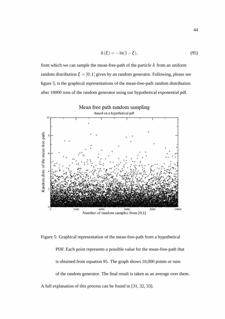
44
λ (ξ ) = − ln(1−ξ ), (95)
from which we can sample the mean-free-path of the particleλ from an uniform
random distributionξ = [0,1[ given by an random generator. Following, please see
figure 5, is the graphical representations of the mean-free-path random distribution
after 10000 runs of the random generator using our hypothetical exponential pdf.
Figure 5: Graphical representation of the mean-free-path from a hypothetical
PDF. Each point represents a possible value for the mean-free-path that
is obtained from equation 95. The graph shows 10,000 points or runs
of the random generator. The final result is taken as an average over them.
A full explanation of this process can be found in [31, 32, 33].

3 Procedures
3.1 Consistency test for the OOS - sum-rule test
Our starting point is the verification of of Bethe’s sum-ruleof the initially available
semi-empirical optical-oscillator-strength-data of aluminum, copper, and gold defined
as [14, 15]
ˆ ∞
0
d f (w,q = 0)
dwdw = Z, (96)
whered f (w,0)dw is the OOS,w is the energy-loss grid,q is the linear momentum transfer,
andZ the number of electrons per atom in the material.
Since the OOS is constructed in part from experiment [25], where index of refraction
and extinction coefficients are used to construct the dielectric function and the energy
loss function of the medium under consideration, please seesection (G) of this
document, and in part with a extrapolation-scheme for the higher-energy shells, this
test verifies if any normalization factor needs to be appliedto the data.
The numerical integration of the OOS is also a good point to verify and optimize the
numerical inrtegration routines. The optimization of the energy loss step sizedw for
the numerical integration in the energy loss domainw was accoplished by force where
direct integration of the OOS as function of step size was done and compared with an
approximately three percent allowed error band with respect to the optimum total
number of atomic electrons that have the well known values of13, 29, and 79,
46
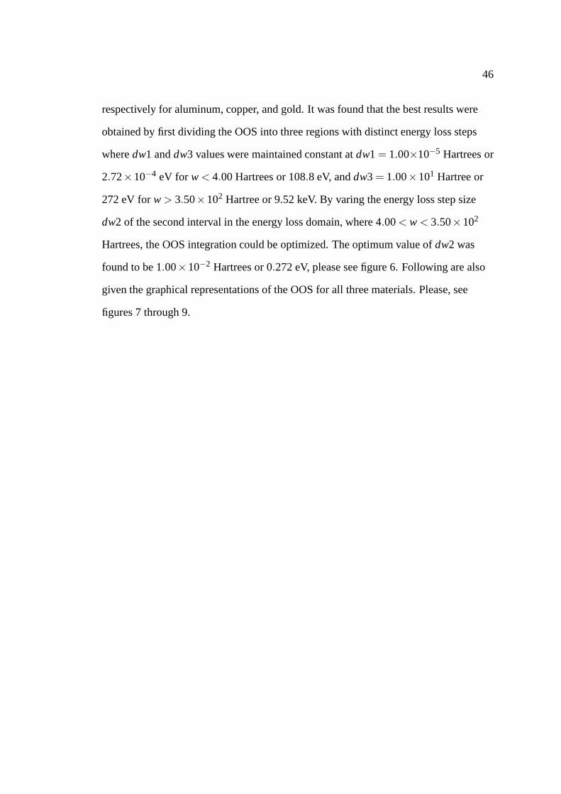
respectively for aluminum, copper, and gold. It was found that the best results were
obtained by first dividing the OOS into three regions with distinct energy loss steps
wheredw1 anddw3 values were maintained constant atdw1 = 1.00×10⁻⁵ Hartrees or
2.72×10⁻⁴ eV for w < 4.00 Hartrees or 108.8 eV, anddw3 = 1.00×101 Hartree or
272 eV forw > 3.50×10² Hartree or 9.52 keV. By varing the energy loss step size
dw2 of the second interval in the energy loss domain, where 4.00< w < 3.50×10²
Hartrees, the OOS integration could be optimized. The optimum value ofdw2 was
found to be 1.00×10⁻² Hartrees or 0.272 eV, please see figure 6. Following are also
given the graphical representations of the OOS for all threematerials. Please, see
figures 7 through 9.
47
Figure 6: Analysis of the integration routine used in the integration of the OOS.
The integration results is shown as function of the energy-loss stepdw2.
The optimum results are values that stay within approximately 3 percent
of the total number of electrons por atom of the target material
(Aluminum Z = 13, copper Z = 29, and gold Z = 79).

48
3.1.1 Aluminum OOS
Figure 7: Optical oscillator strength density distribution of aluminum (Z = 13).
Obtained partially from experimental data [25] and partially from
NIST [26] for w > 1.0 keV.
49
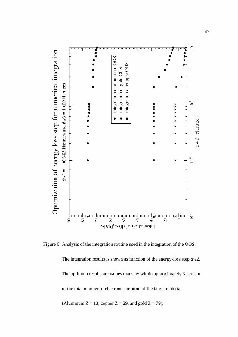
3.1.2 Copper OOS
Figure 8: Optical oscillator strength density distribution of copper (Z = 29).
Obtained partially from experimental data [25] and partially from
NIST [26] for w > 1.0 keV.

50
3.1.3 Gold OOS
Figure 9: Optical oscillator strength density distribution of gold (Z = 79).
Obtained partially from experimental data [25] and partially from
NIST [26] for w > 1.0 keV.

51
3.2 Limits of integration
From the kinematics of the collision we can define the following interval of integration
for the momentum space(qmin,qmax). Recalling the relations between linear
momentum and the energy of the incident particle we can write
qinit =√
2mE (97)
where:qinit is the initial linear momentum magnitude of the incident particle, E the
incident particle’s total kinetic energy, andm its mass.
Now, for a possible loss of energyw during the collision with a target, it is clear that
the incident particle’s magnitude of linear momentum can assume values from a
minimum of
qmin = qinit −q′ =√
2m(√
E −√
(E −w)) (98)
to a maximum of
qmax = qinit +q′ =√
2m(√
E +√
(E −w)) (99)
where:q′ =√
2m(E −w).
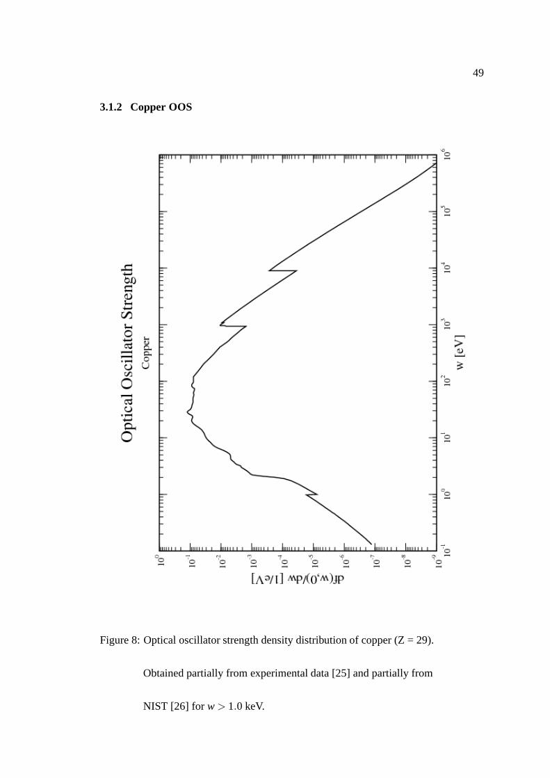
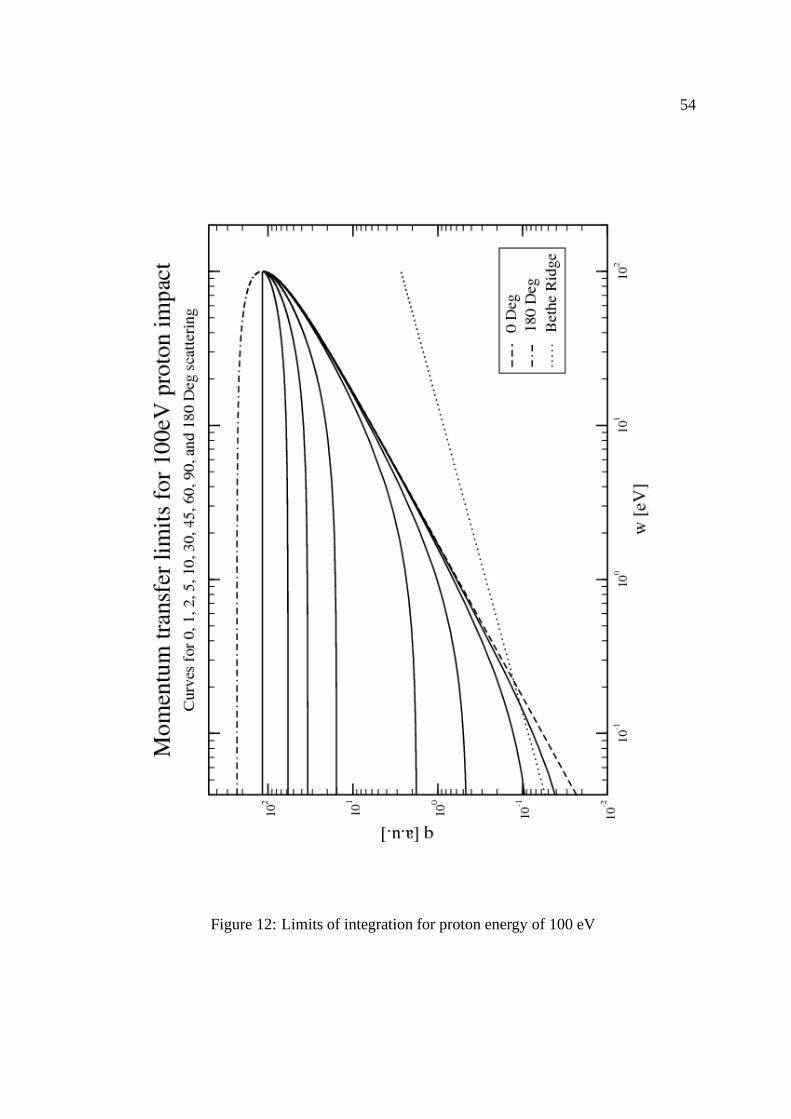
Following are graphical representations of these limits asfunction of energy-loss for
electrons at 10 eV and 1 keV, and proton sources at 100 eV, and 1MeV, please see
figures 10 through 13.

52
Figure 10: Limits of integration for electron energy of 10 eV
53
Figure 11: Limits of integration for electron energy 10 keV
54
Figure 12: Limits of integration for proton energy of 100 eV

55
Figure 13: Limits of integration for proton energy of 10 MeV
56
As expected for the convergence of the integral over linear momentum, see next
paragraph for the calculation of the differential inverse-mean-free-path, the limits
converge to the single valueqmin = qmax =√
2mE asw → E.
Therefore, the first integration of equation 83 defines our first important relation. The
single differential macroscopic cross-section or the differential inverse-mean free-path
(DIMFP) can then be written as
dΣdw
(E;w,q) =1
2a0ZE p2
E1w
ˆ qmax
qmin
1q
d f (w−q2/2)
dwdq (100)
or more conveniently
dΣdw
(E;w,q) =1
2a0ZE p2
E1w
ˆ ρ2
ρ1
d f (w−q2/2)
dwdρ (101)
where:ρ, ρ1,andρ2 are respectively lnq, lnqmin, and lnqmax.
Finally, a second integration over the energy-loss limits defines the other necessary
quantity for the construction of the probability distribution functions for the MC
simulation of the interaction. The inverse-mean-free-path (IMFP) can then be written
as
Σ(E) =1
2a0ZE p2
E
ˆ w
0
1w
dwˆ qmax
qmin
1q
d f (w−q2/2)
dwdq (102)
Note that the IMFPΣ(E) or macroscopic total cross section is related to themicroscopic total cross-sectionσ(E) through the simple relationΣ(E) = Nσ(E),whereN is the number density of the target.
57
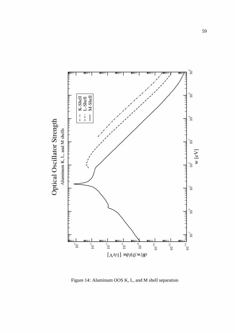
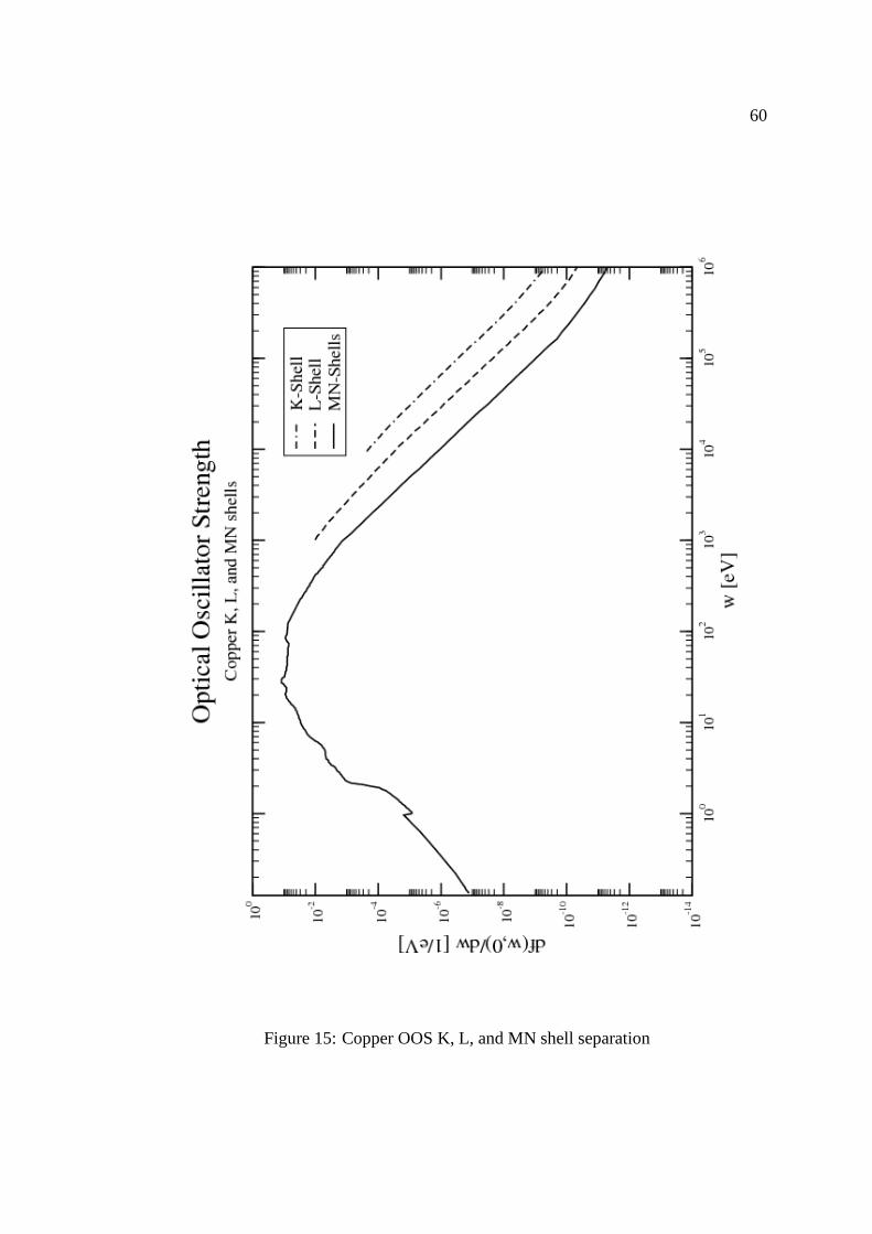
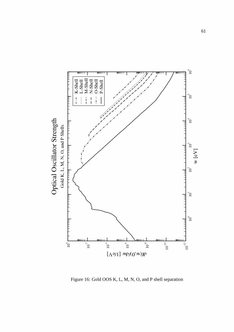
3.3 Shell separation
So far, the calculation of the differential and total cross-sections using the total OOS as
described in figures 7 through 9 respectively for aluminum, copper, and gold returns
the necessary quantities for the MC simulation without providing information about
the initial energy of ejection of the secondary particles inthe case of ionization events.
Similar to the case where the tracking of the primary particles is only possible if we
know, during all the simulation time, the energy and direction of these particles, to
“track” possible secondary electrons, we also need to know their initial energies and
ejection angle distributions.
To fulfill this requirement, the oscillator strength distributions were separated into
shells from where coefficients of proportionality could be introduced and calculated
based on the complete oscillator distribution and sum rules. Following, please see
figures 14 through 16, are the oscillator strength of aluminum, copper, and gold with
their corresponding distribution of oscillators per shell.
Following are also given the edge energies or threshold energies for the corresponding
shells, which were selected to distinct one shell from another. Please note, especially
in the case of gold, that the nomenclature used for the shellsdo not correspond to the
standard classification. This was due to difficulties encountered to distinct the
subshells. Where we say K, L, M, N, O, and P -shells, in the caseof gold, some are
actually sub-shells named L1, L2, and L3 and so on. For our purposes, what is
important for this simulation is to know where the distinctions are made by their
corresponding edge-energies. Specially between what is consider inner and
outer-shells.
58
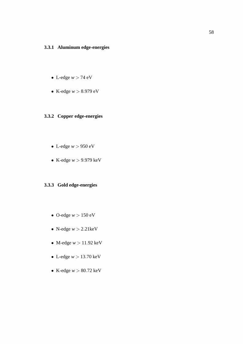
3.3.1 Aluminum edge-energies
• L-edgew > 74 eV
• K-edgew > 8.979 eV
3.3.2 Copper edge-energies
• L-edgew > 950 eV
• K-edgew > 9.979 keV
3.3.3 Gold edge-energies
• O-edgew > 150 eV
• N-edgew > 2.21keV
• M-edgew > 11.92 keV
• L-edgew > 13.70 keV
• K-edgew > 80.72 keV
59
Figure 14: Aluminum OOS K, L, and M shell separation
60
Figure 15: Copper OOS K, L, and MN shell separation
61
Figure 16: Gold OOS K, L, M, N, O, and P shell separation
62
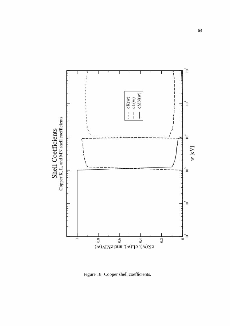
The construction of the shell-coefficients was done in a three step process as follows:
First, a particular shell and its spectrum of participationis identified. In the case of the
aluminum K-shell, its participation starts atw > 8.979 eV , as indicated above.
Second, if other shells overlap in the same energy range, theOOS of the considered
shell is appropriately subtracted from the OOS of these overlaping shells. Finally,
normalization is obtained by dividing the resulting shell-OOS by the total OOS in the
considered spectrum. The result is a coefficient that rangesfrom 0 to 1 that indicates
how strong is the participation of a certain OOS-shell in a particular spectrum. Again
using the aluminum K-shell OOS as an example, we can see that its corresponding
coefficient should be 0 forw < 8.979eV, and assume a value 0< Ck < 1 for
w > 8.979eV. Please, refer to figures 17 through 19 for the completevalues of the
shell-coefficients for aluminum, copper, and gold.
The differential and total cross-sections can then be obtained by multiplying these
coefficients by the previously calculated differential andtotal cross-sections using the
complete oscillator strength distributions. Again, please see figures 17 through 19, for
the graphical representations of the shell-coefficients for aluminum, copper, and gold.
Note that their sum at any point in the spectrum must equal to 1.

63
Figure 17: Aluminum shell coefficients.
64
Figure 18: Cooper shell coefficients.

65
Figure 19: Gold shell coefficients.

66
3.4 Agular distribution of primary and secondary particles
So far, we have considered only the particle’s initial energy and its mean free path for
the determination of their track structure or MC simulation. To complete the modeling
of the simulation of the track-structure of a primary or secondary particle, as they
travel through the target foil, we also need to know the direction that they will take
after an event, elastic or inelastic, takes place. More specifically, we must know their
respective angular probability distribution functions from which the angular variables
θ , andφ can be obtained by appropriate sampling methods. There are four cases to be
considered:
• The angular distribution of fast proton source particles
• The angular distribution of primary electrons that can alsocause further
ionizations
• The angular distribution of secondary electrons induced byelectron impact
• The angular distribution of secondary electron induced by proton impact
3.4.1 Angular distribution of primary protons
For the proton as primary particle, due to its overwhelmingly bigger mass with respect
to the mass of the target electrons (mp ≈ 1836me) and with initial momentumpi also
much greater than the momentum transferq, (pi q), it is then justifiable to consider
that they will approximately travel in straight lines through the material from the
beginning of the simulation to the end. The kinematics resulting in such approximation
follows:
67
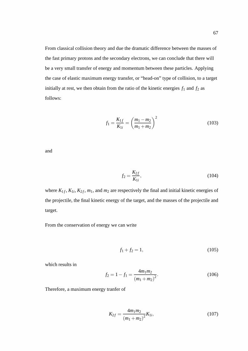
From classical collision theory and due the dramatic difference between the masses of
the fast primary protons and the secondary electrons, we canconclude that there will
be a very small transfer of energy and momentum between theseparticles. Applying
the case of elastic maximum energy transfer, or “head-on” type of collision, to a target
initially at rest, we then obtain from the ratio of the kinetic energiesf1 and f2 as
follows:
f1 =K1 f
K1i=
(m1−m2
m1+m2
)2
(103)
and
f2 =K2 f
K1i, (104)
whereK1 f , K1i, K2 f , m1, andm2 are respectively the final and initial kinetic energies of
the projectile, the final kinetic energy of the target, and the masses of the projectile and
target.
From the conservation of energy we can write
f1 + f2 = 1, (105)
which results in
f2 = 1− f1 =4m1m2
(m1+m2)2 . (106)
Therefore, a maximum energy tranfer of
K2 f =4m1m2
(m1+m2)2K1i, (107)
68
occurs from which we can see that ifm1 m2, K2 f ' 4m2K1im1
K1i.
This lead us to consider for the simulation that the primary fast protons will travel
through the material without being deflected by the target electrons.
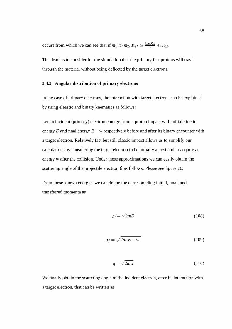
3.4.2 Angular distribution of primary electrons
In the case of primary electrons, the interaction with target electrons can be explained
by using eleastic and binary knematics as follows:
Let an incident (primary) electron emerge from a proton impact with initial kinetic
energyE and final energyE −w respectively before and after its binary encounter with
a target electron. Relatively fast but still classic impactallows us to simplify our
calculations by considering the target electron to be initially at rest and to acquire an
energyw after the collision. Under these approximations we can easily obtain the
scattering angle of the projectile electronθ as follows. Please see figure 26.
From these known energies we can define the corresponding initial, final, and
transferred momenta as
pi =√
2mE (108)
p f =√
2m(E −w) (109)
q =√
2mw (110)
We finally obtain the scattering angle of the incident electron, after its interaction with
a target electron, that can be written as
69
cosθ =E −w√E(E −w)
(111)
Figure 20: Classical scattering kinematics. An incident particle with initial
kinetic energyE loses energyw after its collision with a free electron.
The energyw that is acquired by the target. The incident particle is
scattered in an angleθ with respect to its original trajectory.
3.4.3 Angular distribution of electrons induced by electron impact
In the case of electron-induced emissions, these secondaryelectrons will be emitted at
90o with respect to the direction of the primary electrons. The models are based on
results from experiments involving gas-phase targets and photo-ionization data.
The emission angles for these electrons, known as secondaryelectrons, comes from
two sources:
70
For energy transfersw < 100 eV, the experimental data from Opal et al. [34, 35] were
used. For energy transfersw = 100 eV, non-relativistically, the secondary electron is
emitted perpendicular to the scattered primary electron following approximately
ionization by photon impact where the electrons are ejectedin the direction of the
perpendicular field [36, 37].
3.4.4 Angular distribution of electrons induced by proton impact
Following the steps from Dingfelder et al. in [27] and references therein, the
interaction between the fast protons and the target electrons can be separated into two
types - close or hard collisions and soft collisions due to dipole interactions. This
involving theory is usually called the mixed binary and Bethe theory or binary
encounter dipole model [38].
In summary, it implements or includes the angular dependency into the Bethecoefficients by hand that can be written as
A(w,θ) = A(w). f1(θ) (112)
and
B(w,θ) = B(w). f2(θ) (113)
The functionsf1(θ) and f2(θ) are modelled based respectively on data from
photo-electron emission and binary theory.
3.4.5 Determination of A(w) and B(w)
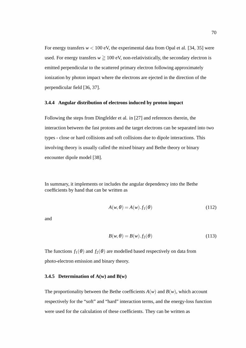
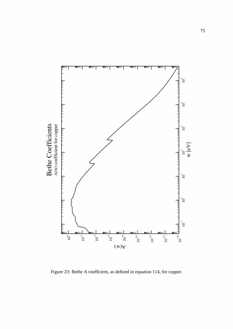
The proportionality between the Bethe coefficientsA(w) andB(w), which account
respectively for the “soft” and “hard” interaction terms, and the energy-loss function
were used for the calculation of these coefficients. They canbe written as

71
A(w) =12
η2(w,0) (114)
and
B(w) =12
η2(w,0)ln
[4(ka0)
2(
Ryw
)2]
+ J1+ J2, (115)
where the auxiliary integralsJ1 andJ2 can be written respectively as
J1(w) =
ˆ ∞
qη2(w,q)
dqq
(116)
and
J2(w) =
ˆ q
0[η2(w,q)−η2(w,0)]
dqq
. (117)
In the auxiliary integralsJ1 andJ2, q is an introduced value, independent ofE, that
separates the high-q and low-q domains. Dingfelder et al. in[27] presents the
complete derivations.
Note that, in the assymptotic region,E w, the First Born approximation differential
cross-section can be substituted by the Bethe differentialcross-section, which can be
written as
dΣdw
=1
πa0E
[A(w) ln
(ERy
)+B(w)+O
(wE
)], (118)
wherea0 is the Bohr radius,w the energy-loss,E the particle’s kinetic energy,Ry is the
Rydenberg energy (13.6 eV). The Bethe total cross-section, after integration of
equation 118, was than used to check our Bethe coefficient calculation results. Please

72
refer to the graphs of the total cross-sections at the end of this document where our
PWFBA calculations are plotted together with the Bethe total cross-sections, which
rely onA(w) andB(w), showing a good agreement in the high energy spectrum.
Finally, to complete the angular profile of the particles, inthis case independent of the
their type, the azimuthal direction is defined by the polar angleφ and obtained from an
uniform distribution in the interval(0,2π) from which random sampling takes place.
Following are the calculated Bethe coefficients for aluminum, copper, and gold based
on their respectively energy-loss functions as previouslydescribed by relations 114,
115, 116, and 117.

73
3.4.6 Aluminum, copper, and gold Bethe coefficients
Figure 21: Bethe A coefficient, as defined in equation 114, foraluminum.

74
Figure 22: Bethe B coefficient, as defined in equation 115, foraluminum.
The B coefficients as indicated by the dashed line are actually
negative in value.
75
Figure 23: Bethe A coefficient, as defined in equation 114, forcopper.

76
Figure 24: Bethe B coefficient, as defined in equation 115, forcopper.
The B coefficients as indicated by the dashed line are actually
negative in value.

77
Figure 25: Bethe A coefficient, as defined in equation 114, forgold.
78
Figure 26: Bethe B coefficient, as defined in equation 115, forgold.
The B coefficients as indicated by the dashed line are
actually negative in value.
4 Results
Finally, we present the complete set of single differentialinverse-mean-free-paths and
the total macroscopic cross sections or inverse-mean-free-paths for electron and proton
impact in isotropic and homogeneous aluminum, copper, and gold thin foils. We also
show the PARTRAC simulation of the forward and backward electron yields from 0.1
micron thick copper foil after a 6 MeV proton impact.
Our calculations using the (PWFBA) are also compared with our calculations using the
Bethe approach and other well known published data. For the inverse mean free path
and stopping power of the foils for electron source the data was compared with results
from Fernandez-Varea. et al. [39, 40]. The proton impact calculations were compared
with well known data from ICRU report 49 [41].
80
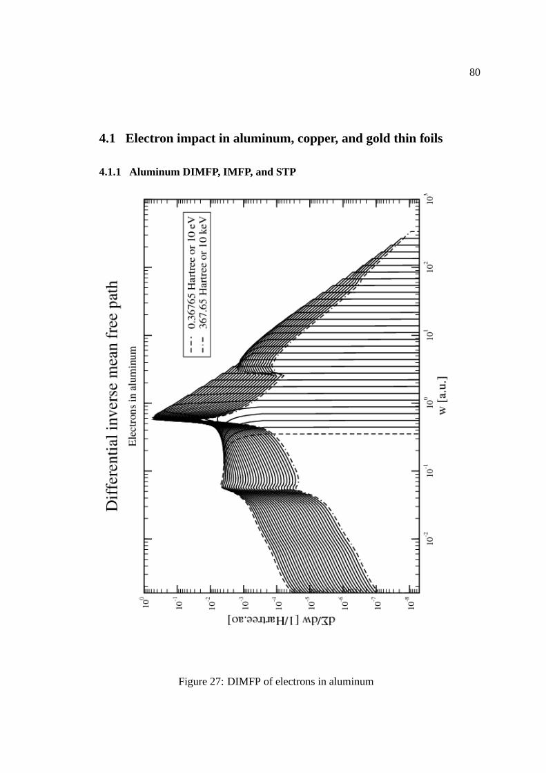
4.1 Electron impact in aluminum, copper, and gold thin foils
4.1.1 Aluminum DIMFP, IMFP, and STP
Figure 27: DIMFP of electrons in aluminum

81
Figure 28: IMFP of electrons in aluminum. Data from
Fernandez- Varea et al. can be found in [39].
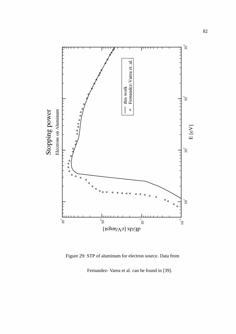
82
Figure 29: STP of aluminum for electron source. Data from
Fernandez- Varea et al. can be found in [39].
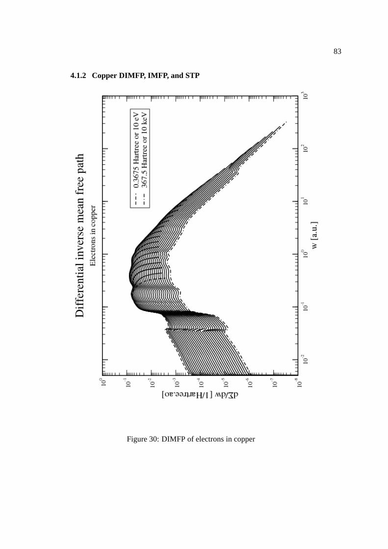
83
4.1.2 Copper DIMFP, IMFP, and STP
Figure 30: DIMFP of electrons in copper

84
Figure 31: IMFP of electrons in copper. Data from
Fernandez- Varea et al. can be found in [39].
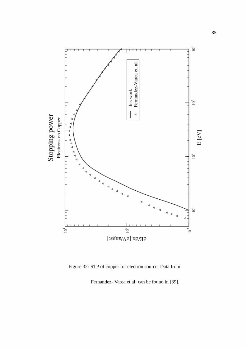
85
Figure 32: STP of copper for electron source. Data from
Fernandez- Varea et al. can be found in [39].

86
4.1.3 Gold DIMFP, IMFP, and STP
Figure 33: DIMFP of electrons in gold
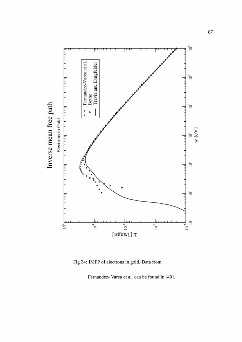
87
Fig 34: IMFP of electrons in gold. Data from
Fernandez- Varea et al. can be found in [40].

88
Figure 35: STP of gold for electron source. Data from
Fernandez- Varea et al. can be found in [40].

89
4.2 Proton impact in aluminum, copper, and gold thin foils
4.2.1 Aluminum DIMFP, IMFP, and mass STP
Figure 36: DIMFP of protons in aluminum
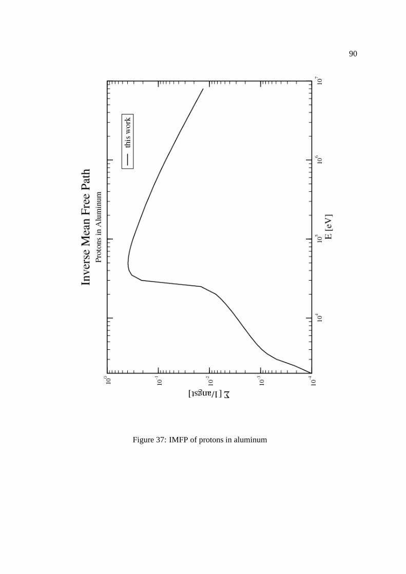
90
Figure 37: IMFP of protons in aluminum

91
Figure 38: Mass STP of aluminum for proton source
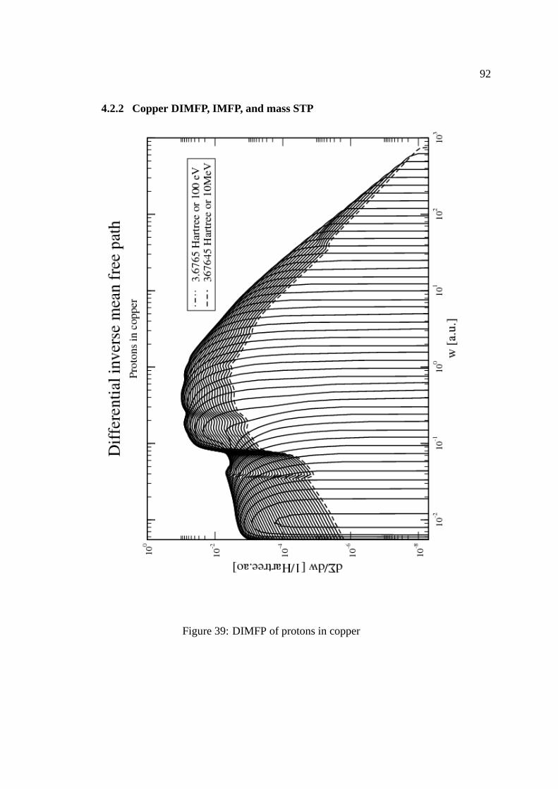
92
4.2.2 Copper DIMFP, IMFP, and mass STP
Figure 39: DIMFP of protons in copper

93
Figure 40: IMFP of protons in copper
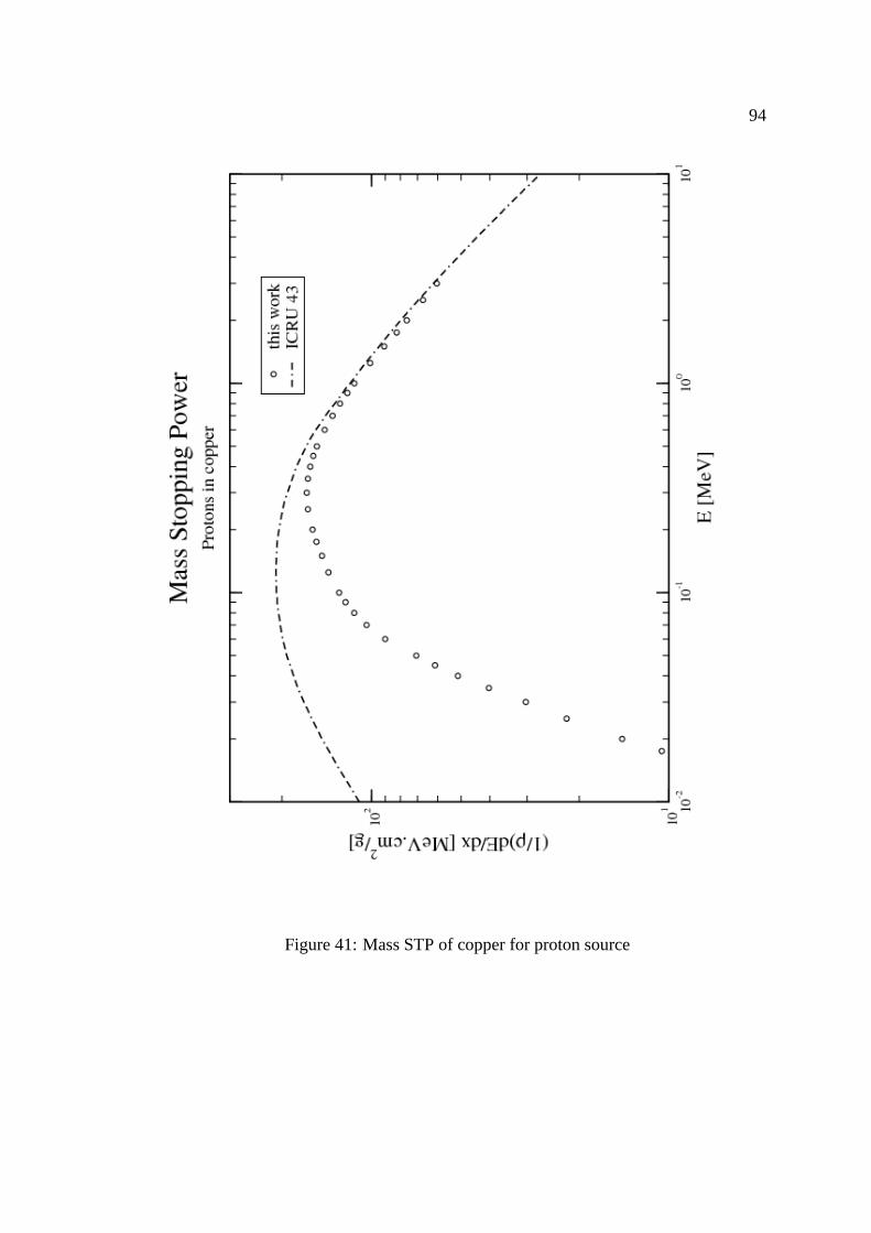
94
Figure 41: Mass STP of copper for proton source

95
4.2.3 Gold DIMFP, IMFP, and mass STP
Figure 42: DIMFP of protons in gold

96
Figure 43: IMFP of protons in gold

97
Figure 44: Mass STP of gold for proton source

98
4.3 Electron yields from 0.1 micron copper foil after 6 MeV proton
impact
4.3.1 Forward electron yields
Figure 45: MC simulation of forward electron yields from copper foil.
Simulation data provided by Dr. Michael Dingfelder.

99
4.3.2 Backward electron yields
Figure 46: MC simulation of backward electron yields from copper foil.
Simulation data provided by Dr. Michael Dingfelder.
5 Conclusion and Remarks
In summary, the simulation of the secondary electron emission from a thin copper foil
after fast proton impact has been accomplished using the Monte Carlo code PARTRAC
after implementation of interaction cross sections calculated from dielectric theory
under the PWFBA. This aloowed us to connect the most important quantity of the
theory, the DDCS, to the GOS through a simple dispersion algorithm known as the
δ -oscillator model and the available OOS of the target. Afterthe DDCS was defined,
the important quantities for the simulation could all be obtained by simple quadrature
numerical methods.
As expected, the results are in agreement within the energy range (> 1 keV for
electron impact and> 1 MeV for proton impact) in which the incident particle is
considerd fast but still nonrelativistic compared with theaverage speed of the target
electrons. Although ourδ -oscillator model includes only the Bethe-ridge or the binary
region of the surface and is clearly not the best representation available of these
targets, equation 81, it satifies the simplicity requirement. It allows a simplification
that is evident from our equation for the GOS and DDCS defined by equations 82 and
83 and obviously the numerical procedures for their implementation.
The continuation of this work could possibly concentrate onimprovements in two
fields:
101
• In the modelling of the Bethe surface of these targets. Rather than using a simple
δ - function, the Bethe-ridge could be expanded with functions (Gaussian type
functions) that allow for a greater momentum exchange interval around the
binary ridge.
• In the numerical implementation - using more dynamical integration routines
that account for pre-defined maximum allowed errors in placeof simple
quadrature schemes.

References
[1] J. E. Turner, Atoms, Radiation, and Radiation Protection (2007), WILEY- VCH
Verlag GmbH & Co. KGaA, Weinheim, ISBN: 978-3-527-40606-7.
[2] G. R. Freeman, Kinetics of Nonhomogeneous Processes - A Practical Introduction
for Chemists, Biologists, Physicists, and Material Scientists (1987), John Wiley &
Sons, Inc., N.Y., ISBN: 0-471-8324-9.
[3] W. A. Glass, and M. N. Varma, Physical and Chemical Mechanisms in Molecu-
lar Radiation Biology, Basic Life Sciences Vol. 58 (1991), Plenum Press, N. Y.,
ISBN: 0-306-44110-1.
[4] M. Zaider, A. Y. C. Fung, J. Li, and J. Ladik, From Track Structure to Stochas-
tic Chemistry and DNA Damage: Microdosimetry Perspective,Inter. Journal of
Quantum Chem., vol 80 (2000), 327-340.
[5] L. H. Toburen, W. Friedland, M. Dingfelder, N. Ozturk, C.Christou, R. D. DuBois,
G. Lapicki, J. L. Shinpaugh, C. G. Drexler, E. L. B. Justiniano, and H. G. Paret-
zke, Secondary Electron Production and Transport Induced by Fast Protons in
Thin Foils, Application of Acc. in Research and Industry: 17th Int’l. Conference
(2003), Am. Inst. of Phys., 0-7354-0149-7/03.
[6] J. D. Jackson, Classical Electrodynamics (1999), John Wiley & Sons, Inc., ISBN:
0-471-30932.
[7] L. Eyges, The Classical Electromagnetic Field (1972), Dover Publications, N. Y.,
ISBN: 0-486-63947-9.
[8] D. Atwood, Soft X-rays and Extreme Ultraviolet Radiation (1999), Cambridge
University Press, ISBN:0-521-65214-6.
[9] G. R. Fowles, Introduction to Modern Optics (1989), Dover Publications, Inc., N.
Y., ISBN:0-486-65957-7.
103
[10] M. L. Boas, Mathematical Methods in The Physical Sciences (1983), John Wiley
& Sons, Inc., ISBN: 0-471-04409-1.
[11] G. B. Arfken and H. J. Weber, Mathematical Methods for Physicists (2001), Har-
court Academic Press, ISBN: 0-12-059825-6.
[12] M. Fox, Optical Properties of Solids - Oxford Master Series in Condensed Matter
Physics Vol.I (2001), Oxford University Press Inc., N. Y., ISBN: 0198506120.
[13] L. D. Landau, E. M. Lifshitz, and L. P. Pitaevskii, Electrodynamics of Contin-
uous Media - Landau and Lifshitz Course of Theoretical Physics Vol. 8 (1984),
Pergamon Press Ltd., ISBN: 0-08-030276-9.
[14] M. Inokuti, Inelastic Collisions of Fast Charged Particles with Atoms and
Molecules - The Bethe Theory Revisited (1971), Rev. of Mod. Phys. 43 (3), 297-
347.
[15] M. Inokuti, Y. Itikawa, J. E. Turner, Addenda: Inelastic collisions of fast charged
particles with atoms and molecules (1971) [Rev. Mod. Phys. 43, 297] – The Bethe
theory revisited, Rev. of Mod. Phys. 50 (1), Part I (1978), 23-35.
[16] H. A. Bethe, R. Jackiw, Intermediate Quantum Mechanics(1986), Westview
Press, ISBN: 0-201-32831-3.
[17] E. Fermi, The Ionization Loss of Energy in Gases an in Condensed Materials
(1940), Phys. Rev. 57, 485.
[18] J. Hubbard, The Dielectric Theory of Electronic Interactions in Solids (1955),
Proc. Phys. Soc. A 68, 976-986.
[19] U. Fano, Penetration of Protons, Alpha Particles, and Mesons (1963), Ann. Rev.
Nucl. Sci. 13, 1-66.

104
[20] K. L. Bell, D. J. Kennedy, and A. E. Kingston, Excitationof helium by fast elec-
trons (1968), J. Phys. B (Proc. Phys. Soc.), ser. 2, vol. 1.
[21] K. L. Bell, D. J. Kennedy, and A. E. Kingston, Excitationof helium by fast protons
(1968), J. Phys. B (Proc. Phys. Soc.), ser. 2, vol. 1.
[22] A. Szabo, and N. S. Ostlund, Modern Quantum Chemistry - Introduction to Ad-
vanced Electronic Structure Theory (1982), Dover Publications, Inc., N.Y., ISBN:
0-486-69186-1.
[23] D. B. Cook, Handbook of Computational Quantum Chemistry (1998), Dover Pub-
lications N. Y., ISBN: 0-486-44307.
[24] D. Emfietzoglou, A. Pathak, and M. Moscovitch, Modelingthe energy and mo-
mentum dependent loss function of the valence shells of liquid water (2005), Nucl.
Instr. and Meth. in Phys. Res. B 230, 77-84.
[25] E. D. Palik, Handbook of Optical Constants of Solids (1985), Academic Press
Inc., N. Y., ISBN: 0-12-544420-6.
[26] NIST, National Institute of Standards and Technology -Physics Laboratory,
http://physics.nist.gov/PhysRefData/Xcom/html/xcom1.html
[27] M. Dingfelder, D. Hantke, M. Inokuti, and H. G. Paretzke, Electron inelastic-
scattering cross sections in liquid water (1998), Rad. Phys. and Chem. 53, 1-18.
[28] M. Dingfelder, M. Inokuti, H. G. Paretzke, Inelastic-collision cross sections of
liquid water for interactions of energetic protons (2000),Rad. Phys. and Chem.
59, 255-275.
[29] N. W. Ashcroft, N. D. Mermin, Solid State Physics (1976), Thomson Lerning Inc.,
ISBN: 0-03-083993-9.

105
[30] J. C. Ashley, Optical-data model for the stopping powerof condensed matter for
protons and antiprotons (1991), J. Phys.: Condens. Matter 3, 2741-2753.
[31] M. Dingfelder, R. H. Ritchie, J. E. Turner, W. Friedland, H. G. Paretzke, and R.
N. Hamm, Comparisons of Calculations with PARTRAC and NOREC: Transport
of Electrons in Liquid Water (2008), Rad. Res. 169, 584-594.
[32] M. H. Kalos and P. A. Whitlock, Monte Carlo Methods, vol.1 (1986), Jon Wiley
& Sons, Inc., N.Y., ISBN:0-471-89839-2.
[33] F. Salvat, J. M. Fern ´andez-Varea, E. Acosta, and J. Sempau, PENELOPE - A Code
System for Monte Carlo Simulation of Electron and Photon Transport (2001),
Workshop Proceedings Issy-les-Moulineaux, France, ISBN:92-64-18475-9.
[34] C. B. Opal, E. C. Beaty, and W. K. Peterson, Tables of Energy and Angular Distri-
butions of Electrons Ejected from Simple Gases by Electron Impact, Report No.
108, Joint Institute for Laboratory Astrophysics (JILA), Boulder, CO, (1971).
[35] C. B. Opal, E. C. Beaty, and W. K. Peterson, Tables of secondary electron produc-
tion cross sections, Atomic Data 4, 209 (1972).
[36] M. Dingfelder, Cross section calculations in condensed media: charged particles
in liquid water, Rad. Protec. Dosim. 99, Nos 1-4, (2002) 23-28.
[37] Y. -Ki Kim, Angular Distribution od secondary electrons in the dipole approxima-
tion, Phys. Rev. A. 6, No 2, (1972) 666-670.
[38] Y. -Ki Kim and M. Eugene Rudd, Binary-encounter-dipolemodel for electron-
impact ionization, Phys. Rev. A. 50 (5), (1994), 3954-3967.
[39] J. M. Fern ´andez-Varea, R. Mayol, F. Salvat, and D. Liljequist, A comparison onf
inelastic electron scattering models based onδ -function representations of the
Bethe surface, J. Phys.: Condens. Matter 4 (1992) 2879-2890.

106
[40] J. M. Fern ´andez-Varea, R. Mayol, D. Liljequist, and F. Salvat, Inelastic scattering
of electrons in solids from a generalized oscillator strength model using optical
and photoelectric data, J. Phys.: Condens. Matter 5 (1993) 3593-3610.
[41] ICRU Report 49, Stopping power and ranges for protons and alpha particles, In-
ternational Commission on Radiation Units and Measurements.