and Coastal and Modeling Systems: A New Frontier in ...godae-data/School/Chapter04... · 91 CHAPTER...

91

C H A P T E R 4

Shelf and Coastal Ocean Observing and Modeling Systems: A New Frontier in

Operational Oceanography Moninya Roughan1,2,3, Colette Kerry2, and Peter McComb1

1MetOcean Solutions and New Zealand MetService New Zealand; 2 School of Mathematics and Statistics,

University of New South Wales, Sydney NSW, 2052, Australia; 3 School of Biological, Earth and Environmental Sciences, University of New South Wales, Sydney NSW, 2052, Australia

One of the new frontiers in operational oceanography includes progress in observing and modeling the coastal ocean. In addition to this, it is becoming increasingly important to bring operational oceanographic data to industry in a usable format. We use the case study of Australia’s Integrated Marine Observing System (IMOS) and its application to the East Australian Current to introduce some of the latest ideas about shelf and coastal ocean observing and modeling, and its applications to operational oceanography.

Introduction and Motivation

oastal oceans are among the most productive ecosystems on the planet, providing an array

of services that directly and indirectly support economic activity and growth. In addition

to the plethora of ecosystem services, social and environmental benefits, our coastal

oceans provide services of great economic value including: protection from natural hazards;

weather regulation; shoreline stabilization; carbon sequestration; wild-catch fisheries; energy from

wind, waves and offshore oil; sea bound trade; and tourism. These services, along with many others,

provide the foundation for an estimated $3–$5 trillion dollars in annual global ocean economic

activity (http://www.pemsea.org/our-work/blue-economy).

Indeed, in some Asian countries it is estimated that up to 20-30% of their Gross Domestic

Product (GDP) comes from the ocean (http://www.pemsea.org/our-work/blue-economy), while

Australia has one of the world’s largest Exclusive Economic Zones (EEZs) providing a total value

of over $70 billion and more than 400,000 jobs (2013-14, http://www.aims.gov.au/aims-index-of-

marine-industry). Continental shelf regions are even more important economically. Even though

only a small percentage of the surface area of the world oceans is comprised of these regions, they

provide between 15 and 30 % of the entire oceanic primary production (Yool and Fashman, 2001).

Presently about 40% of the world’s population lives within 100 km of the coast, and in some

countries, such as Australia, this figure can be as high as 80%

Roughan, M., C. Kerry, and P. McComb, 2018: Shelf and coastal ocean observing and modeling systems: A new frontier in operational oceanography. In "New Frontiers in Operational Oceanography", E. Chassignet, A. Pascual, J. Tintoré, and J. Verron, Eds., GODAE OceanView, 91-116, doi:10.17125/gov2018.ch04.

C

9 2 M O N I N YA R O U G H A N E T A L .

(http://www.un.org/esa/sustdev/natlinfo/indicators/methodology_sheets/oceans_seas_coasts/pop_

coastal_areas.pdf). As population density and economic activity in coastal zones increases,

pressures on coastal ecosystems increase.

Moreover, a country’s EEZ extends up to 200 nautical miles from its coastline, thus individual

nations and broader groups such as the European Union (EU) have an impetus to understand their

coastal ocean domains. An adequate understanding of the coastal marine environment is

fundamental to manage it sustainability. However, we are presently limited in our ability to measure

and model our marine environments, particularly at scales sufficient for resolving the dynamics of

the coastal ocean.

In recognition of the significance of our coastal and shelf regions, a range of long-term observing

initiatives have been developed over the past 1-2 decades. In the U.S., coastal ocean observing

programs emerged through a bottom-up approach, where local counties, universities, and

organizations began sustained observing. In the absence of regional coordination, these groups grew

into a network of regional alliances (e.g., see Chapter 21 by Wilkin et al.) brought together into a

nationally coordinated way under the Integrated Ocean Observing System (IOOS) framework. In

Australia, sustained ocean observing was instigated through a series of tranches of federal funding

to support the Integrated Marine Observing System (IMOS, www.imos.org). This resulted in a

nationally coordinated network of oceanographic observations for the coastal and deep ocean.

In the ocean modeling space, the experiences of the U.S. and Australian regional alliances also

differ substantially. The U.S. has led the way in ocean modeling, both in development of open

source ocean models (such as POM, ROMS, and FVCOM) as well as in implementation in

operational oceanography and the application to regional alliances. In contrast, Australian modeling

initiatives were not funded through the “ocean observing” program, which has meant that the

application of coastal observations in an operational ocean hindcasting or forecasting framework

has been more ad hoc.

To date, Australia’s ocean modeling needs have been serviced by the BlueLink project, which

provides circulation at 10 km resolution (Oke et al., 2008). However, near-global models, such as

these with 7–10 km resolution, are insufficient for resolving flow in the coastal ocean (e.g., along

southeastern Australia where the shelf is <30 km wide in many places). Notably, in addition to

insufficient resolution, near-global models, including BlueLink, exclude important coastal

processes, such as tidal forcing, local winds, and river input.

There are very few countries globally that have high resolution operational ocean forecasting

capability. Presently, the Australian Bureau of Meteorology and the Commonwealth Scientific and

Industrial Research Organisation (CSIRO) have coastal capability in only two regions (the Great

Barrier Reef and the Great Australian Bight) driven by end user and stakeholder needs. Despite this,

significant efforts are being undertaken in the ocean observing space in the coastal ocean, and it is

the integration of these modeling and observing efforts that are the leading edge in operational

oceanography.

Here we present the example of the New South Wales node of the Australian Integrated Marine

Observing System (NSW-IMOS) and showcase the benefit of sustained ocean observations in the

S H E L F A N D C O A S T A L O C E A N O B S E R VI N G A N D M O D E L I N G S Y S T E M S : A N E W F R O N T I E R I N O P E R A T I O NA L O C E A N O G R A P H Y 93

coastal ocean as a pathway for operational oceanography in our shelf sea. In the context of

operational oceanography, there is unlimited potential to develop coastal operational hindcasting

and prediction systems, which is clearly one of the new frontiers in operational oceanography and

coastal modeling.

Observing the Coastal Ocean: Australia’s Integrated Marine Observing System (IMOS)

Boundary currents (BCs) are highly energetic regions of our ocean basins that redistribute water,

heat, and salt around the globe. As such, BCs play a major role in regulating the global climate

system and they have a profound influence on local ocean and weather processes. Yet monitoring

the multi-space and timescales of the energetic dynamic flows of boundary currents can be

complicated.

One of the next frontiers in operational oceanography is development and implementation of a

global network designed for sustained monitoring of our BCs in order to understand their full multi-

scale variability from time and space scales that span from sub-seasonal to multi-decadal and from

turbulent to basin scales; moreover we need to understand the interaction of BCs with marginal

seas, frontal processes that aid mixing and cross front flows, and air-sea interaction, as well as their

impacts on marine ecosystems.

Along the east coast of Australia, significant effort has been put into sustained monitoring of

the East Australian Current (EAC, the Western boundary current of the South Pacific Ocean) and

its interaction with shelf waters (Fig. 4.1). This has been facilitated since 2006 through IMOS

(www.imos.org.au). In the IMOS framework, funding flows through ‘centralized facilities’ that are

responsible for the deployment of the ocean observing “kit” such as high frequency (HF) radar,

autonomous gliders, and moorings (deep and shallow). Whereas the science is driven by regional

“nodes” that are a loose grouping of scientists united under a coordinated science and

implementation plan (http://imos.org.au/plans.html). There are three IMOS nodes that contribute to

our understanding of the EAC: two coastal nodes that together cover the entire east coast of

Australia (Q-IMOS and NSW-IMOS) and a blue water and climate node which encompasses the

offshore regions around Australia. Over the past ten years, a comprehensive ocean observing

network has been deployed and refined with the purpose of understanding the dynamics of the

WBC, its impact on shelf circulation, and biological productivity.

Since 2006, the Australian federal government has invested more than $190 million in IMOS,

with an additional co-investment of 140% from industry, universities, stakeholders, state and federal

agencies. The main goal is to provide a multidisciplinary, multi-institutional approach to enhance

the observation and understanding of the oceans around Australia. The funding flows through ten

centrally coordinated “infrastructure” facilities that are responsible for deploying ocean observing

equipment in both the coastal and deep ocean, to measure a number of physical, chemical, and

biological variables. These facilities are supported by the national IMOS office and an eleventh data


facility responsible for management and free distribution of the data, the Australian Ocean Data

Network (AODN, www.aodn.org.au).

Figure 4.1. Sea surface temperature (SST) image (AVHRR SST L3 for 7 June 2015) showing the East Australian Current flowing poleward along the east coast of Australia. Color indicates SST and identifies the WBC jet, the Tasman front and the EAC eddy field.

Science objectives

The infrastructure deployment around Australia has been driven by a series of science questions

that are documented in the IMOS Node Science and Implementation Plans

(http://imos.org.au/about/about-imos/plansreports/). Through this process, a number of unifying

national overarching goals were identified: 1. multi-decadal ocean change, 2. climate variability

and weather extremes, 3. major boundary currents and inter-basin flows, 4. continental shelf and

coastal processes, and 5. the ecosystem response. In the context of coastal oceanography, there are

two main objectives:


1. To investigate the East Australian Current, its separation from the coast and the resultant

eddy field in order to:

determine the statistical, dynamic, and kinematic properties of EAC eddies, and the

frequency and dynamical drivers of eddy shedding;

quantify the impact of key physical processes driven by the EAC such as onshore

encroachment, shelf circulation driven by the EAC, cross shelf processes, and internal

waves; and

understand air-sea interactions, particularly to determine the development of east

coast lows and severe winter storms in relation to warm core eddies and oceanic

conditions.

2. To quantify oceanographic processes on the continental shelf and slope of southeastern

Australia in order to:

examine the coastal wind and wave climate in driving nearshore currents and the

northward sediment transport;

quantify the biogeochemical cycling of carbon (nutrients and phytoplankton

composition); and

determine the transport and dispersal of passive particles (e.g., larvae, eggs, spores)

and the degree of along-coast connectivity and trophic linkages.

Ocean observing infrastructure

To provide insight into these science objectives in the context of coastal Australia, three coastal

focal regions were chosen: Coffs Harbour (30oS), Sydney (34oS), and Narooma (36oS). Coffs

Harbour lies approximately 550 km to the north of Sydney, while Narooma lies approximately

350km to the south. In addition, a full-depth transport resolving array was deployed from the

continental shelf off Brisbane to 150 km offshore at about 27.5°S. These are the only permanent

mooring along an approximately 2000 km stretch of coastline, and not a single one has a surface

expression for real-time or air-sea fluxes and over-ocean wind measurements. These arrays are

described below and outlined in Fig. 4.2.

Deep water moorings

In an effort to resolve the full-depth transport of the EAC, a mooring array was deployed across

27.5°S where the EAC has been shown to be most coherent. Seven moorings were deployed in

water depths of 200 to ~4800 m over a distance of ~153 km from the continental shelf to the abyssal

plain (See Fig. 4.2 and Sloyan et al., 2016, Table 1). Q-IMOS, the coastal node of IMOS responsible

for observing northern Australia, deployed the shelf moorings in 200 and 400 m of water. The deep-

water moorings were deployed shore normal to this array across the continental slope and abyssal

moorings by the IMOS deep water mooring program as part of the Bluewater and Climate

Observing node (BWC). The moorings were instrumented with Teledyne RD Instrument (TRDI)

acoustic Doppler current profilers (ADCPs) of various frequencies (e.g., 75, 150, and 300 kHz),

which provided velocity profiles at varying vertical resolution from 4 to 16 m, in the upper 1000 m

in a range of configurations. In addition, point-source velocity data were obtained from Nortek


Aquadopp instruments at varying vertical resolution of 500 to 1000 m. In addition, 55 point-source

temperature sensors and 25 point-source salinity sensors (Sea-Bird Electronics) were distributed

across the seven moorings. In total, 143 instruments were deployed across the array. See Sloyan et

al. (2016) for further details of the mooring program and instrumentation.

Figure 4.2. Location of the observing infrastructure along the coast of southeastern Australia. This includes deep water moorings (off Brisbane at ~27.5°S) and shelf moorings, HF coastal radar, biogeochemical sampling, wave rider buoys and example tracks from autonomous ocean gliders (where Nemo are shelf missions < 200m, and Dory are deep missions < 1000m). Insets from top to bottom (right) show the moorings at Coffs Harbour, Sydney and Narooma. Not shown are satellite remote sensed data, Argo floats and repeat XBT lines (shown in Fig. 4.4). 100 m, 200 m (bold) and 2000 m contours are shown. Note the HF radar array at 33oS shows representative coverage only.

The mooring array was deployed for an 18-month period from April 2012 to August 2013

(Sloyan et al., 2016). Then, due to funding constraints, was removed for a two-year period. The

array was consolidated into six moorings and redeployed in May 2015.

These data were used to understand the mean velocities, coherence of the EAC, and the transport

of heat and mass. Mean velocities calculated from the18-month time series show poleward velocity

from the 0 to 1500 m adjacent to the continental shelf, with a recirculation feature offshore. While

the EAC has been shown to exhibit variability on a range of timescales and a degree of incoherence,

this dataset showed that the EAC was coherent during this time at this latitude, with an eddy kinetic

to mean kinetic energy ratio of less than 1.


Moreover, they calculated the 18-month mean, poleward-only mass transport above 2000 m to

be 22.1 ± 7.5 Sv (where 1 Sv is 106 m3 s−1). The mean, poleward-only heat transport and flow-

weighted temperature above 2000 m were −1.35 ± 0.42 PW and 15.33°C, respectively.

Using the results of a complex empirical orthogonal function (EOF) analysis of the along-slope

velocity anomalies, Sloyan et al. (2016) further showed that velocity variance is dominated by two

modes of variability at periods of approximately 60 days (Mode 1) and 120 days (Mode 2), and

together they explain more than 70% of the velocity variance.

Shelf moorings

A network of up to ten coastal moorings has been deployed in shelf waters from 65-140 m deep

along the coast of southeastern Australia since 2008 (Fig. 4.2). The moorings were deployed in

shore-normal arrays in each of the three coastal focal regions: Coffs Harbour (30oS), Sydney (34oS),

and Narooma (36oS). The moored array was designed to build upon existing operational

observations e.g., a hydrographic mooring supported by Sydney Water Corporation off Sydney

(ORS065) since 1991, and a network of wave rider buoys measuring wave height and direction

funded by NSW state government (Fig. 4.2). The ORS065 dataset has been collected operationally

on behalf of Sydney Water Corporation as part of their license to operate an offshore sewage ocean

outfall since 1991. This is one of the longest moored full water column temperature records

available around Australia, and it exists entirely due to operational necessity.

The moorings have existed in a number of different configurations over the years, however,

presently the moorings consist of a bottom-mounted TRDI 300kHz ADCP and a string of Aquatech

520 temperature and temperature/pressure loggers at 8 m intervals through the water column (Table

1, Roughan et al., 2013, 2015). The line of thermistors is supported by a float, approximately 20 m

below the surface. Below the sub-surface float at PH100 is a Wetlabs water quality meter (WQM)

that consists of a SeaBird CTD, as well as measurements of dissolved oxygen, fluorescence, and

turbidity (Wetlabs FLNTU). The WQM is being phased out and replaced with a SeaBird SBE37

CTD at the bottom and below the surface (See Roughan et al., 2015, 2013, 2011 for further details).

Needless to say, over-ocean winds are an important component of any observing system as they

provide validation for atmospheric forcing products. In this region, very limited over-ocean wind

observations have been available historically, however, modeled products perform reasonably well

(Wood et al., 2012). Another alternative for broad-scale wind patterns are satellite-derived

observations and products, which have been shown to perform well in this region (Rossi et al.,

2014).

In regions of strong currents (such as the EAC), it is challenging to deploy moorings with a

surface expression that would hold atmospheric sensors; however, this is becoming more feasible

as technology improves. Associated with a mooring that has a surface expression is the ability to

telemeter data in real time. Thus, development of a real-time data delivery system is the next

obvious improvement to the array, which will support operational purposes as well as real-time

validation of model output.


Autonomous ocean gliders

Between 2008 and 2017, 32 autonomous ocean glider missions were undertaken along the coast of

southeastern Australia. Typically, these missions spanned the continental shelf on the inshore edge

of the EAC from 29.5–33.5°S. The region is both physically and biologically significant, and it is

in a hotspot of ocean warming. This comprehensive dataset of over 40,000 new CTD profiles from

the surface to within 10 m of the bottom in water depths ranging 25–200 m provides unprecedented

high resolution observations of the properties of the continental shelf waters adjacent to a western

boundary current, straddling the region where it separates from the coast. The dataset consists of

temperature, salinity, and density, as well as dissolved oxygen and chlorophyll-a fluorescence

(indicative of phytoplankton biomass).

The data have been released publically in a gridded dataset (Schaeffer et al., 2016a) and are an

invaluable resource with which to understand shelf circulation dynamics (Schaeffer and Roughan

2015), stratification (Schaeffer et al., 2016b, Schaeffer and Roughan 2015), biophysical and bio-

geochemical interactions (Baird et al., 2011; Everett et al., 2015; Schaeffer et al., 2016b). They are

also useful for data assimilation into and validation of high-resolution ocean models (Kerry et al.,

2016). Moreover, the data are being used as teaching material for ocean observing classes

introducing students to the newest methodology and procedures in ocean observing.

Using the combined gridded dataset, Schaeffer et al. (2016b) calculated the spatial scales of

variability on the continental shelf—showing the anisotropy in the EAC in both the physical and

biogeochemical datasets. These data are useful in the context of ocean data assimilation, where

errors need to be prescribed to the data prior to assimilation (see following section and Kerry et al.,

2016).

High frequency coastal radar

A pair of high frequency (HF) coastal radars (Wellan Radar) were installed at 30oS off southeastern

Australia in February 2012. The phased array system remotely measures surface currents in the top

0.9 m off Coffs Harbour (Eastern Australia, 30°S–31°S; Fig. 4.2). This HF system operates at

13.92MHz frequency, with radial and azimuthal resolutions of 1.5 km and 10.4°, respectively

(Wyatt et al., 2017). It acquires data every 10 minutes with an offshore range of up to 150 km (see

Wyatt et al., 2017; Mantovanelli et al., 2017; Archer et al., 2017, and Schaeffer et al., 2017 for more

details of the system deployment and data validation).

Cyclonic eddies that form on the inside edge of the WBC have been shown to entrain coastal

waters (Everett et al., 2015; Macdonald et al., 2016; Roughan et al., 2017). Schaeffer et al. (2017)

presented results from an automated eddy detection algorithm applied to the radar surface currents

over a one-year period and showed that cyclonic eddies are generated on average every seven days

on the inside edge of the EAC.

High frequency measurements of over-ocean wind direction and surface currents were used by

Mantovanelli et al. (2017) to reveal the influence of the short-term, small-scale wind forcing on the

surface circulation, enhancement of horizontal shear, frontal jet destabilization, and the generation

and decay of a cyclonic eddy.


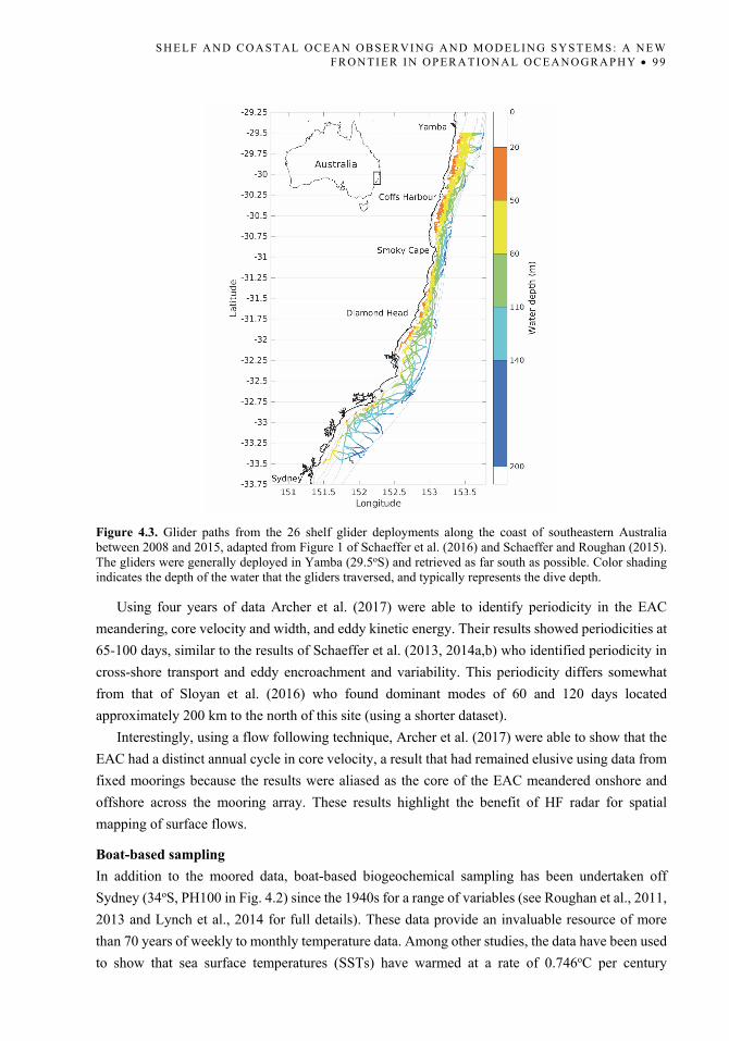
Figure 4.3. Glider paths from the 26 shelf glider deployments along the coast of southeastern Australia between 2008 and 2015, adapted from Figure 1 of Schaeffer et al. (2016) and Schaeffer and Roughan (2015). The gliders were generally deployed in Yamba (29.5oS) and retrieved as far south as possible. Color shading indicates the depth of the water that the gliders traversed, and typically represents the dive depth.

Using four years of data Archer et al. (2017) were able to identify periodicity in the EAC

meandering, core velocity and width, and eddy kinetic energy. Their results showed periodicities at

65-100 days, similar to the results of Schaeffer et al. (2013, 2014a,b) who identified periodicity in

cross-shore transport and eddy encroachment and variability. This periodicity differs somewhat

from that of Sloyan et al. (2016) who found dominant modes of 60 and 120 days located

approximately 200 km to the north of this site (using a shorter dataset).

Interestingly, using a flow following technique, Archer et al. (2017) were able to show that the

EAC had a distinct annual cycle in core velocity, a result that had remained elusive using data from

fixed moorings because the results were aliased as the core of the EAC meandered onshore and

offshore across the mooring array. These results highlight the benefit of HF radar for spatial

mapping of surface flows.

Boat-based sampling

In addition to the moored data, boat-based biogeochemical sampling has been undertaken off

Sydney (34oS, PH100 in Fig. 4.2) since the 1940s for a range of variables (see Roughan et al., 2011,

2013 and Lynch et al., 2014 for full details). These data provide an invaluable resource of more

than 70 years of weekly to monthly temperature data. Among other studies, the data have been used

to show that sea surface temperatures (SSTs) have warmed at a rate of 0.746oC per century

1 00 M O N I NY A R O U G H AN E T A L .

(Thompson et al., 2009) off Port Hacking, Sydney, Australia. More recently, Schaeffer and

Roughan (2017) used the data to create a daily temperature climatology for the region, which they

used in conjunction with the high resolution mooring data to investigate the sub-surface structure

and dynamics of marine heatwaves (MHWs) over the past 20 years. Their results showed that

MHWs are subsurface intensified and are longer below the surface. These data are becoming

increasingly essential and make a valuable contribution to operational oceanography, model

verification and validation (discussed further below).

Model‐Data Integration to Improve Operational Outcomes

Without a doubt, the next ten years will see a range of advances in ocean modeling and the

integration of observational data at increasing resolution, particularly in coastal areas. As the coastal

zone is where societal necessities are greatest, there is a pressing need for accurate, detailed, and

timely information on the marine environment at increasing resolutions. In Australia, the Australian

Bureau of Meteorology/CSIRO presently provides coastal forecasts for the Great Barrier Reef at 4

km resolution (www.ereefs.org.au). However, like most countries, Australia currently depends on

a global operational ocean forecasting system of ~10 km (1/12o) resolution (BlueLink, Oke et al.,

2008) for forecasts along the majority of its coastline. Many developed countries, such as New

Zealand, do not have their own ocean forecasting system and thus they rely on products developed

by other nations, also at about 10 km resolution (e.g., the U.S. Navy implementation of Global

HYCOM, Chassignet et al. (2009), and Mercator Ocean of France, www.mercator-ocean.fr). The

relatively coarse resolution of global models, required at present due to computational limitations,

makes them inappropriate for coastal-scale prediction where they are unable to resolve the complex

bathymetry and submesoscale processes. Along the coast of southeastern Australia, for example,

the continental shelf is narrow (~15-30 km wide) and is not well-resolved at 10 km resolution.

While the global operational ocean forecasts presently available resolve the typically slowly

evolving, synoptic, mesoscale flows, regional and coastal models resolve smaller temporal and

spatial scales that are more rapidly evolving and have shorter decorrelation timescales. For slowly

evolving flows, data assimilation schemes that assume all data to be at the analysis time can be

effectual; the global BlueLink reanalysis and forecast system uses ensemble optimal interpolation

(Oke et al., 2008; Oke et al., 2013), while HYCOM uses 3D-Var (Cummings, 2005). Mercator

Ocean of France uses a data assimilation system based on the singular evolutive extended Kalman

(SEEK) filter (Brasseur and Verron, 2006). These data assimilation techniques proceed only

sequentially and do not optimize the fit between observations and model over the full extent of the

assimilation window. This makes them ill-suited to highly intermittent flows, typical of non-

synoptic scales in the coastal ocean, with irregularly sampled observations. Indeed, these techniques

are no longer used in numerical weather prediction (e.g., Lorenc and Rawlins, 2005). The two

techniques that are now the most promising in numerical weather prediction are 4D-Var and the

ensemble Kalman filter (EnKF), which consider the time-evolving model state in the data

assimilation methodology. 4D-Var and EnKF are considerably more computationally expensive but


are becoming viable for regional ocean forecasting. In the ocean, 4D-Var is used by select groups

for regional forecasts (e.g., the Pacific Islands Ocean Observing System, the Mid-Atlantic Coastal

Ocean Observing System, and the Central and Northern California Ocean Observing System, all in

the U.S.), while the EnKF is used operationally in the Great Barrier Reef, Australia

(www.ereefs.org.au).

With the step change in observations available in the coastal ocean, it behooves us to extend our

operational models into the coastal ocean. The coastal and continental shelf region of southeastern

Australia, the country’s most densely populated region, has been well-observed over the past ten

years. While these observations have been very useful in understanding coastal and continental shelf

processes, such as cross-shelf dynamics (Schaeffer et al., 2013), upwelling (Schaeffer et al., 2014;

Schaeffer and Roughan, 2015) and frontal eddies (Schaeffer et al., 2017). They have largely not

been exploited for operational forecasting purposes. To make use of southeastern Australia’s coastal

observing system and provide coastal forecasts we need to develop a high resolution data

assimilating model of the coastal ocean.

A high‐resolution reanalysis of the East Australian Current

As a first step towards integrating the array of observations described above into an operational

model, we perform a two-year case study assimilating all of the available observations into a shelf-

resolving model. For the region dominated by the EAC, we combine a high-resolution state-of-the-

art numerical ocean model with a variety of traditional and newly available observations using an

advanced variational data assimilation scheme. The southeast Australian coastal ocean provides an

ideal study site for this research as it exhibits complex shelf dynamics, is impacted by an intense

WBC, and there are a large number of observations on the shelf.

We begin by configuring a numerical model of the oceanic region off southeastern Australia

(domain shown in Figs. 4.4a and 4.4b) that is capable of representing the mean ocean circulation

and its eddy variability. We configure the model using the Regional Ocean Modeling System

(ROMS 3.4) and provide boundary forcing from the BlueLink ReANalysis (BRAN3, Oke et al.,

2008, 2013), the Australian operational hindcast. The model has a variable horizontal resolution in

the cross-shore direction, with 2.5 km over the continental shelf and slope that gradually increases

to 6 km in the open ocean and a resolution of 5 km in the along-shore direction. The variable

resolution allows us to resolve the continental shelf, which is 15 km wide at its narrowest point,

while avoiding excessive computational expense. This work is described in detail in Kerry et al.

(2016).

In order to correctly represent the spatial and temporal evolution of the eddy field, we need to

constrain the model with observations. For the data assimilation, we use an Incremental Strong-

Constraint 4-Dimensional Variational (IS4D-Var) scheme (Moore et al., 2004, 2011a). This

technique uses the (linearized) model dynamics to compute increments in the initial conditions,

atmospheric forcing, and boundary conditions, such that the difference between the new model

solution and the observations is minimized (in a least squares sense) over an assimilation window,

given prior assumptions of the uncertainties in the observations and the model background state.


The new modeled ocean state (the reanalysis) better fits and is in balance with the observations. The

assimilation is performed over five-day windows as, for this model configuration, the linear

assumption remains acceptable for typical perturbations over five days.

The reanalysis is configured for the two-year period of 2012-2013 because of the availability of

significant observational resources during this time; in particular, a deep water mooring array

deployed to capture the transport of the EAC (described above and in Sloyan et al., 2016). In

addition to the traditional data streams (satellite derived sea surface height (SSH) and SST, Argo

profiling floats, and XBT lines), we exploit many of the newly available observations that were

collected as part of IMOS. These include velocity and hydrographic observations from the above-

mentioned deep water mooring array and several moorings on the continental shelf, surface radial

current observations from a HF radar array, and hydrographic observations from ocean gliders (Fig.

4.4). The SSH observations are from the Archiving, Validation and Interpretation of Satellite

Oceanographic Data (AVISO) daily gridded Sea Level Anomaly product and the SST data is from

the U.S. Naval Oceanographic Office Global Area Coverage Advanced Very High Resolution

Radiometer level-2 product. For details of the observations and their processing before integration

into the assimilation system, refer to Kerry et al. (2016).

Figure 4.4. Observations used in the two-year reanalysis from 2012-2013. Argo observations colored by time of occurrence, (a), and all other observations, with the exception of satellite-derived SSH and SST, (b). 100m, 200m and 2000m contours are shown. HF radar sites Red Rock (RRK) and North Nambucca (NNB) are shown with black asterisks in (b) and zooms showing the percent coverage of radial data for the two stations are shown in (c) and (d). Number of observations (after processing) from each observation platform used in each five-day assimilation window are shown in (e). Adapted from Kerry et al. (2016).


Figure 4.5. Time series of spatially-averaged RMS SSH observation anomaly, RMS SSH difference between the free run and observations, RMS SSH difference between the analysis and observations, and RMS SSH difference between the forecast and observations, for each assimilation window (a). As above but for SST (b). RMS potential density observation anomaly and RMS difference between the free run and observations, the analysis and observations, and the forecast and the observations for glider observations (c). As above but for Argo observations (d) and for independent CTD cast observations (e). Locations of the CTD casts are shown in the inset in (e). The blue, green and magenta dots represent CTD casts taken on different cruises over the two-year period. Adapted from Kerry et al. (2016).

The reanalysis is shown to represent both assimilated and non-assimilated observations well.

The system achieves mean spatially-averaged Root Mean Squared (RMS) residuals between the

analysis and the observations of 7.6 cm for SSH and 0.39oC for SST over the assimilation period.

The mean RMS residual between the forecast and the observations are 9.8 cm for SSH and 0.55oC

for SST. Figs. 4.5a and 4.5b show the time series of the spatially-averaged RMS observation

anomalies and RMS residuals between the free-running model and the observations, the analysis

and the observations and the forecasts and the observations for each 5-day window over the 2-year

reanalysis for SSH and SST, respectively. For SSH, the free-running model’s residuals with the

observations are of similar order to the observation anomalies (which represent the SSH variability),

indicating that the model has very little skill in predicting SSH without data assimilation. For SST,

the free-running model has some skill; the root-mean-square deviations (RMSDs) between the free


run and the observations are lower than the SST observation anomalies. For both SSH and SST, the

analyses and forecasts show significantly improved representation of the observations, compared

to the free-running model.

Both Argo floats and ocean gliders measure subsurface temperature and salinity, allowing

potential density to be computed. Figs. 4.5c and 4.5d show profiles of the RMS potential density

observation anomaly and RMS difference between the free run and observations, the analysis and

observations, and the forecast and the observations for glider observations and Argo float

observations, respectively. For Argo, the peak in the RMS residual between the analysis and the

observations occurs at about 60-100 m and is 0.23 kgm-3, with an increase to 0.28 kgm-3 for the

residual between the forecast and the observations. The majority of the glider observations are taken

on the continental shelf and shelf slope, and the forecasts degrade more rapidly from the analyses

(compared to the Argo observations, which mostly sample the offshore deep water region). At their

peak (100 m depth), the RMS residual between the analysis and the glider observations is 0.21 kgm-

3, and the residual with the forecasts is 0.37 kgm-3.

Comparison with independent (non-assimilated) shipboard CTD cast observations shows a

marked improvement in the representation of the subsurface ocean in the reanalysis, with the RMS

residual in potential density reduced to about half of the residual with the free-running model in the

upper eddy-influenced part of the water column (Fig. 4.5e). This shows that information is

successfully propagated from observed variables to unobserved regions as the assimilation system

uses the model dynamics to adjust the model state estimate.

Velocities at several offshore and continental shelf moorings are well-represented in the

reanalysis, with complex correlations between 0.8-1 for all observations in the upper 500 m (not

shown). Surface radial velocities from the HF radar array are assimilated and the reanalysis provides

surface velocity estimates with complex correlations with observed velocities of 0.8-1 across the

radar footprint (not shown). An example of the improvement in surface current representation

achieved by assimilation of the HF radar data is shown in Fig. 4.6 for the assimilation window

beginning on March 14, 2012. The surface velocities computed from the assimilated HF radar

observations of the radial components of the surface currents (Fig. 4.6a) show a recirculation feature

with northward flow inshore of the dominant southerly flow. This is not represented in the forecast

(Fig. 4.6b), but is present upon assimilation (Fig. 4.6c). The corresponding SSH observations,

model forecast, and analysis are shown in Figs. 4.6d-f. The anticyclonic eddy that is in balance with

the observed currents is not present in the assimilated SSH observations (which are only used further

than 100 km from the coast), but becomes present in the analysis SSH field.

This is the first study to generate a reanalysis of the region at such a high resolution, making use

of an unprecedented observational dataset and using an assimilation method that uses the time-

evolving model physics to adjust the model in a dynamically consistent way. The reanalysis

provides a good representation of the ocean state, as measured by both the assimilated and non-

assimilated observations. The RMS residuals with the observations remain low in the subsequent

five-day forecasts for the SSH, SST, and Argo float observations. However, the forecasts have

considerably greater residuals for the glider observations, most of which are taken close to or over


the continental shelf. Likewise, as seen in the example in Fig. 4.6, small-scale circulation features

on the shelf are often not captured in the forecasts.

From an operational forecasting perspective, this system is likely to be effective for mesoscale

type forecasts, but would require further tuning and/or downscaling to provide accurate predictions

close to the coast or on the shelf and shelf slope. Some of the considerations when downscaling to

increasingly higher resolutions are discussed in the next section. Also, many of the observations

used are not available in real time. Understanding which observations are important in informing

the model, and therefore are worth making available operationally, is a key step towards developing

an effective forecasting system for this region.

Figure 4.6. Example of one particular assimilation window (March 14, 2012) showing the impact of the assimilation of the HF radial component of surface velocity. Surface velocity vectors computed from assimilated surface radial currents, with current speed shown in color bar (a), model forecast velocities (b) and analysis velocities (c). SSH-assimilated observations (d), model forecast SSH (e) and analysis SSH (f). The box represented by the dashed line in (b)-(f) shows the area of (a), which has different axis limits to show the surface velocities computed from the observed radial velocities more clearly.


Understanding observation impact

Given the significant investment required to install and sustain ocean observations, and to make the

data available in real time, it is important to understand which observations (locations and variables)

are most useful in informing our models. This allows one to assess the cost–benefit of each

observation stream and design an observing system that can be applied for operational purposes to

provide effective forecasts.

Various methods have been used to assess the impact of observations on model predictions. Oke

and Sakov (2012) used satellite-derived SSH and SST and model output to assess the footprint of

mooring observations around Australia based on zero time-lag correlations. This general approach

is not dependent on a specific model or data assimilation configuration and provides a useful

assessment of the moorings' effectiveness in monitoring the circulation, but is limited in that it does

not consider multivariate correlations or time-lags. Observing System Experiments (e.g. Oke and

Schiller, 2007; Oke et al., 2015), in which observations are systematically withheld, are useful to

assess the relative importance of various observations; however, these experiments are unable to

quantify the value of the observations given the complete assimilation system, as when some

observations are withheld the value of the remaining observations changes.

A particularly useful method of assessing observation impact is Observing System Simulation

Experiments (OSSEs, e.g., Schiller et al., 2004; Tranchant et al., 2008). By defining a given model

solution as the true state, these experiments allow us to assimilate synthetic observations (i.e.,

simulated observation types and locations that are constructed from model output to assess their

utility) and investigate predictive skill based on a known ocean state. The goal is to assimilate

observations extracted from the true state, with realistic errors applied, into a predictive model

allowing one to assess how well the assimilation improves the model estimates. The true state can

be chosen as a different model realization of the same time period, a coarser model, or even the

same model, in which case the forecast model is initialized from a perturbed initial state. Synthetic

observations can be withheld to establish the impact of each observing system. Such experiments

are useful as we can compare our estimates to a known state, as compared to prediction studies of

the real ocean using actual observations in which the ocean state is largely unknown.

The influence of synthetic observations can also be assessed using a representer-based approach

(e.g., Zhang et al., 2010; Powell, 2017), which requires the adjoint and tangent-linear versions of

the ocean model. This method shows how individual observations project onto the ocean state,

which reveals the area and relative magnitude of the observations' influence. For example, this

method was used by Zhang et al. (2010) to study the influence of observations on circulation in the

New York Bight and show that regular glider transects influence a greater area than a profiling

mooring, but the mooring has a stronger influence at its particular location.

A unique advantage of variational data assimilation methods is that they can reveal the

dynamical connections between model fields through the use of the tangent-linear and adjoint

models (Moore et al., 2004). In solving the state estimation problem with 4D-Var, one computes

the dynamical covariance between the observations and the model that allows direct computation

of the impact of each observation on the change in circulation estimate between the forecast and the


analysis (as described in Moore et al., 2011b). This method was used by Powell (2017) to show that

ocean glider observations are particularly impactful in constraining transport in the Hawai’i Lee

Countercurrent. Moore et al. (2011b) used 4D-Var to assess observation impact in the California

Current and described a method to determine the sensitivity of circulation estimates to changes in

the observations, providing a way of estimating the change in the analysis due to degradation or

failure of an observation platform.

In order to make specific decisions on observing system design, we need to undertake targeted

studies specifically designed to determine optimum observations given specific prediction goals.

Such experiments should quantify the potential benefits of making different observations and make

recommendations for optimizing the deployment of expensive assets in our present observing

system.

Downscaling and data assimilation at increasingly higher resolution

Fine-scale predictability of the coastal ocean is a new frontier in operational oceanography. With

increased computational resources and model efficiency, there is an increasing push towards

providing forecasts that resolve even finer scale features in coastal regions, such as submesoscale

dynamics, coastal upwelling, shelf fronts, and filaments. However, the predictability of the coastal

ocean is not yet well-understood.

Errors in ocean modeling can arise from uncertainties in initial conditions and model error,

which is composed of a number of factors including grid resolution, numerics, atmospheric forcing,

boundary conditions, and parameterization of physical processes. While errors in initial conditions

dominate at the beginning of the forecast window, as the forecast length grows model error

dominates the forecast skill. Operational ocean forecasts available at present typically resolve the

slowly evolving mesoscale circulation (with model resolutions of about 10 km), which is highly

sensitive to the initial state, and data assimilation methods typically focus on minimizing the error

in the initial state at the beginning of each analysis window. However, with improved model

resolution and physics, model error increases more rapidly. This so-called “curse of resolution”

stems from the fact that finer grid resolution and numerics increase the model error by resolving

finer scales of short period turbulence that have faster error growth. As such, prediction of finer-

scale oceanic processes presents additional challenges as the modelled circulation is likely to be

more rapidly decoupled from the initial state and depend strongly on surface and boundary forcing

and model parameters.

In order to develop accurate forecasting systems, we need to first understand the sensitivity of

the forecast skill to uncertainty in the initial conditions, model forcing, and model parameters.

Indeed, for a downscaled coastal model where processes strongly depend on boundary conditions

and surface forcing, using data assimilation to update the initial conditions may provide little value.

Configuring a well-tuned, free-running model and using data assimilation for parameter estimate

may be more effective.


Framework for model inter‐comparison

One of the major limitations in comparing model performance internationally is that there is no

single set of metrics nor is there a consistent observational framework with which to assess models.

This is further complicated by different data formats, e.g., mean dynamic topographies, time

averaging (daily means etc.), and no consistent file naming convention. This has been recognized

as a limitation in the GODAE global ocean data assimilation experiment task team who have

proposed an inter-comparison framework as documented in Martin et al. (2013). To encourage

global best practices, we suggest adopting the GODAE guidelines to ensure international operability

from the outset. Furthermore, this will ensure future modeling efforts will feed back into global

assessment programs. Importantly, coastal observations are needed for model assessment and

validation. For example, assessment can be against observations that have been withheld (such as

shipboard CTD casts, glider surveys, HF radar velocities, etc.) depending on the experiment. Thus,

good dialogue is required between the observing and modeling communities.

The Need for Operational Oceanography in the Coastal Ocean: Case Study of Marine Heatwaves and Aquaculture.

In this section, we introduce new research into marine heatwaves (MHWs), a very recent area of

research in coastal oceanography. This research has been facilitated by access to long-term datasets

of ocean temperature, which in this case were collected originally for operational purposes at the

Ocean Reference Station (see Fig. 4.2, Sydney insert). We then introduce an aquaculture example

and explore operational considerations for fish farming in the coastal ocean, in the context of ocean

warming.

Marine heatwaves

Analogous to atmospheric heatwaves, MHWs are defined as discrete, prolonged anomalously warm

water events, lasting more than five days (Hobday et al., 2016). Extremely hot SSTs have become

more common in one-third of the world’s coastal areas over the past 30 years (Lima and Wethey,

2012). In recent years, MHWs have become more common in the coastal ocean and they are having

unprecedented biological impacts including mass mortality and habitat shifts.

In response to severe thermal stress, marine communities have to either acclimatize or move to

more suitable (cooler) habitat either further poleward or deeper. This includes not only shallow

communities but also benthic species, some coral communities, and seaweed below the surface

mixed layer (Schaeffer and Roughan, 2017). Increasingly, habitat-forming species are dying during

MHWs and they are not able to recover after an MHW has subsided (Wernberg et al., 2016). In

order to sustainably manage our coastal oceans into the future, we need to understand both long-

term trends in ocean warming, as well as the characteristics of events such as MHWs.

Off western Australia, a severe MHW event occurred during the 2010-2011 austral summer,

lasting over a month; with anomalies up to 5oC above the climatological mean (Pearce and Feng,


2013). Wernberg et al. (2016) showed that two years after the event the cool water kelp forests had

not recovered, and there was a community-wide shift towards warm water seaweeds and fish.

However, little is known about the characteristics of MHWs due to the lack of long-term in situ

observations.

While satellite derived data such as SST can be used to identify broad spatial patterns in MHWs,

the time series is only 30 years and the data are only representative of the sea surface. Because

Schaeffer and Roughan (2017) had access to long-term high resolution moored temperature

information (5-minute data at 4-8 m resolution through the water column, since 1991 off Sydney at

the ORS065 site as described above, see also Fig. 4.2), they were able to characterize the MHWs

that have occurred in the region over the past 20 years.

Using this valuable dataset in conjunction with temperature climatology for the region,

Schaeffer and Roughan (2017) were able to show that MHWs are sub-surface intensified, and

appear to be driven by local wind forcing. Downwelling winds force the warm water downward,

resulting in a maximum peak right below the thermocline. In contrast, upwelling favorable winds

are able to arrest the temporal evolution of the MHW. The data also showed that SST underestimates

the peak intensity and duration of MHWs off the coast of southeastern Australia because of their

sub-surface intensification. Little is known about temperature extremes at depth due to the lack of

long-term in situ measurements so this is an area that needs more observational effort.

Salmon aquaculture

From an operational perspective, one of the industries that is presently being impacted by ocean

warming and MHWs is the salmon aquaculture industry. Salmon farming is a highly lucrative

industry, with salmon products in increasingly high demand. In Australia, the Tasmanian salmon

farming industry is worth ~$550 million AUS per year, and is projected to be a billion-dollar

industry within 20 years as it is rapidly surpassing other fisheries. Chile is the second largest

exporter of salmon and their industry is worth over $4.5 billion (USD) p.a., and in New Zealand,

salmon aquaculture is worth about $50-$70 million pa.

Salmon cannot regulate their body temperature and thrive when water is between 12-17oC.

When water temperatures rise, salmon cardiovascular capacity is lowered, fish become more

vulnerable to disease and predators, and if temperatures get too high it can be fatal. Less

catastrophic, but still an operational consideration, is the impact of water temperature on

consumption. Salmon slow down their eating when temperatures rise, and increase when water is

cooler. Thus, water temperature has an impact on how much feed a company requires.

Globally rising temperatures and MHWs are having severe consequences on the salmon

aquaculture industry. During early 2016, the salmon industry in Chile experienced $800 million

(USD) in losses (100,000 tons lost) with sea temperatures 2-4oC above average for a prolonged

period of time and recurrent harmful algal blooms.

In the austral summer of 2015, water temperatures stayed above 18oC for three months in the

Marlborough Sounds of central New Zealand. Large numbers of salmon died in the Marlborough

Sounds creating a "multimillion-dollar problem" for the New Zealand salmon industry.


Operational considerations of MHWs and the salmon aquaculture industry

In recent years, ocean temperatures off Tasmania (southern Australia) and New Zealand have been

regularly exceeding 18oC in summer. This raises a number of questions with operational

implications, such as: What are the long-term temperature trends? What is driving the increase in

temperature? Is it in situ heating, anomalous air sea fluxes, advection, reduced mixing or a

combination of mechanisms?

Once the in situ temperature datasets are long enough, we can begin to assess trends in MHWs

and correlate climatology with salmon losses. There is a pressing need to understand if MHWs are

increasing in frequency, duration and or intensity. The results of Schaeffer and Roughan (2017)

showed that MHWs were sub-surface intensified off the east coast of Australia. However, we don’t

know the implication of sub-surface intensification on the salmon aquaculture industry. What we

do know is that the salmon pens in Marlborough Sound New Zealand extend ~24 m below the

surface, which may impact salmon health if MHWs are sub-surface intensified in this region.

Finally, off southeastern Australia, Schaeffer and Roughan (2017) showed that MHWs had an

average duration of 8-12 days but could last for over month. This is sufficient time to have an impact

on marine life, particularly on organisms that live below the surface. However, the question

remains: how long is too long and how do these timeframes differ from organisms such as microbes

and plankton to larger more developed organisms such as fish?

Operational decision timescales

For operational purposes, there are three main timescales on which decisions need to be made;

therefore, pertinent information is required within these three timeframes in mind to facilitate the

decision-making process. The timeframes are:

1. Weather timescales, typically 1–7 days. With minimal warning, typically the only

management option is reactive management.

2. Seasonal timescales, 2 weeks–9 months. This timeframe gives an early window for

implementation of strategies with which to minimize impacts and maximize opportunities.

3. Climate forecasting, 10–100s of years. This timeframe serves for long-term planning

purposes and future proofing of the industry.

The seasonal timescale is the most useful for proactive management. Business performance and

industry resilience could be improved with prediction about future conditions.

Benefits of public–private partnerships

There is no doubt that there have been many benefits from the public–private partnerships in

sustained ocean observing. One example along the coast of southeastern Australia is the long ocean

temperature time series at the Ocean Reference Station (ORS) provided by the Sydney Water

Corporation (SWC, see Fig. 4.2). This data is collected on behalf of SWC as part of their license to

operate a deep water ocean sewage outfall. SWC requires information on the ocean stratification


and velocities to drive a plume dispersion model. This data provider has strict key performance

indicators against it, as such the data quality are extremely high including, on average, a more than

90% data return over the past ten years. SWC has generously made this data available to the

scientific community through the ocean data portal, which has facilitated a whole range of research

opportunities. In addition, by opening up the dataset the research community has been able to build

on their efforts by augmenting the data collection through two additional moorings forming a cross

shelf array, anchored in the near shore by the ORS. In other instances, where data has not been

released publically, data collection efforts are often duplicated, sometimes knowingly.

Operational Data Delivery

Increasingly, industry end users are requiring sophisticated tools to access display and analyze

meteorological and oceanographic data. Moreover, many industry end users of oceanographic data

prefer a one stop shop data and model display platform to streamline their operations. As coastal

hindcast and forecast modeling becomes more sophisticated with assimilation at high resolution,

and more real-time data streams become available, these platforms will be necessary to deliver real-

time operational data streams to users.

Figure 4.7. Example screen shot from the MetOceanView (MOV) platform showing wave heights (m) through Bass Straight (southern Australia) for operational purposes. Note the complex scenario through the straight where waves are coming from both directions and are interacting with the topography.

Traditionally, the barriers to this path have been timely access to data and the experience of the

people involved. When an expert (e.g., a weather forecaster) is inserted into the decision-making

process, the operational context is often lost and numerous simplifications need to be made. The net

result can be conservative and insufficiently quantitative for modern logistics, with the justification

being that people are busy and need only the distilled result without all the detail. The contrary view

is that people are intelligent and can make wise decisions if provided the correct information and

empowered with tools to create project-specific knowledge.


Recognition for improved operational decision-making is at the core of the global move toward

providing the common operational picture at an organizational level. Typically delivered within

GIS architecture, these systems display assets alongside the spatial gradients in the important

environmental variables. Time can be applied as a fifth dimension, allowing forecast or hindcast

data to be accessed seamlessly. Further, with or without a common operational picture framework,

many industry end users still require a web-delivered service to access, display, and analyze

meteorological and oceanographic data. The goal is a one-stop platform to streamline their

operations.

Figure 4.8. Screen shot from the MOV data display platform showing real-time weather observations displayed alongside the forecast predictions (left), and presentation of the full population of forecast ensembles with customized probabilistic measures (right).

There are a growing number of examples of services that cater to this need, and one of the more

mature is the MetOceanView (MOV) platform developed by MetOcean Solutions in New Zealand

(www.metoceanview.com). This is a web-delivered, map-based tool that allows customized user

access to a wide range of marine weather variables along with some tools to display and integrate

those data (see Fig. 4.7 for an example). The underlying architecture of MOV is a series of API

micro-services, which allow a spectrum of service delivery levels – either via the dedicated MOV

web service or integration into an existing dynamic GIS platform or static monitoring display

system.

The original concept for MOV was first developed in 2006, with the aim of creating an offshore

construction project resource where users would have unlimited and instant access to all the relevant

marine observations, forecasts, and hindcasts in one place. By opening up all the datasets and

displaying them to everyone on the project, the project team members became highly skilled users

over time. Their feedback led to the development of a suite of tools and ways of displaying data for

rapid inclusion in the decision-making process. Two good examples are displaying real-time

weather observations alongside the forecast predictions (Fig. 4.8, left) and presentation of the full

population of forecast ensembles with customized probabilistic measures (Fig. 4.8, right).


The coastal zone is the area of greatest interest to industry users. Here too, the spatial gradients

in oceanographic variables are typically the highest and their temporal changes of larger

consequence. Coastal modeling is meeting those needs with more sophisticated solutions;

unstructured model domains, and real-time data assimilation at high resolution are becoming

operational norms. The challenge is how to let users engage meaningfully with these new and

important data sources. Without question, it requires dialogue and deep involvement between the

scientists, developers, and the end users. Finally, a key consideration is to ensure delivery platforms

are not built as monolithic structures unable to cope with new observational datasets and evolving

model outputs. Keeping systems flexible will allow for future integration and ingestion of new and

increasingly larger datasets. In this way, we ensure that end users have access to the data needed to

ensure safe and efficient operations.

Acknowledgments

MOV figures provided by Simon Weppe. The operational decision timescales were adapted from C. Spillman personal communication. IMOS is supported by the Australian Government through the National Collaborative Research Infrastructure Strategy and the Super Science Initiative and the Education Infrastructure Fund. CK is partially funded through and Australian Research Council Discovery Project to MR (ARC DP140102337). We acknowledge the vast contribution made by the IMOS technical staff and fieldwork teams including the NSW-IMOS moorings team, the ANMN, ANFOG, ACORN, and ABOS facilities.

References

Archer, M. R., Roughan, M., Keating, S. R., Schaeffer, A., 2017: On the variability of the East Australian Current: Jet structure, meandering, and influence on shelf circulation. J. Geophys. Res. Oceans, 122, 8464–8481. https://doi.org/10.1002/2017JC013097.

Baird, M.E., I. M. Suthers, D. A. Griffin, B. Hollings, C. Pattiaratchi, J. D. Everett, M. Roughan, K. Oubelkheir, M. Doblin. 2011: The effect of surface flooding on the physical-biogeochemical dynamics of a warm-core eddy off southeast Australia. Deep Sea Research II, 58, 592–605.

Brasseur, P. and Verron, J., 2006: The SEEK filter method for data assimilation in oceanography: a synthesis. Ocean Dynamics, 56, 650-661.

Chassignet, E.P., H.E. Hurlburt, E.J. Metzger, O.M. Smedstad, J., G.R. Halliwell, R. Bleck, R. Baraille, A.J. Wallcraft, C. Lozano, and others. 2009: US GODAE: Global Ocean Prediction with the HYbrid Coordinate Ocean Model (HYCOM). Oceanography, 22(2), 64–75.

Cummings J A., 2005: Operational Multivariate Ocean Data Assimilation. Q. J. R. Meteorol. Soc., 131, 3583–3604

Everett, J. D., H. S. Macdonald, M.E. Baird, J. Humphries, M. Roughan, I. M. Suthers, 2015: Cyclonic entrainment of pre-conditioned shelf waters into a Frontal Eddy. J. Geophys. Res. Oceans, 120, doi:10.1002/2014JC010301.

Hobday, A. J., et al. 2016: A hierarchical approach to defining marine heatwaves. Prog. Oceanogr., 141, 227–238, doi:10.1016/j.pocean.2015.12.014.

Kerry, C. G., B. Powell, M. Roughan and P. Oke 2016: Development and evaluation of a high-resolution reanalysis of the East Australian Current region using the Regional Ocean Modeling System (ROMS 3.4) and Incremental Strong-Constraint 4-Dimensional Variational data assimilation (IS4D-Var). Geosci. Model Dev., 9, 3779-3801, doi:10.5194/gmd-2016-44.

Lima, F., and D. Wethey 2012: Three decades of high-resolution coastal sea surface temperatures reveal more than warming, Nat. Commun., 3, 1–13, doi:10.1038/ncomms1713.

Lynch, T.P., Morello, E.B., Evans, K., Richardson, A., Rochester, W., Steinberg, C. R., Roughan, M., Thompson, P., Middleton J. F., Feng, M., Sherrington, R., Brando, V., Tilbrook B., Ridgway, K., Allen, S., Doherty, P., Hill, K., Moltmann, T.C.Z. 2014: IMOS National Reference Stations: A continental scale


physical, chemical, biological coastal observing system. PLoS ONE, 9(12): e113652, doi:10.1371/journal.pone.0113652.

Lorenc A. C. & Rawlins F. 2005: Why does 4D-Var beat 3D-Var? Quarterly Journal Royal Meteorological Society, 131, 3247-3257, doi: 10.1256/qj.05.85.

Macdonald, H. S., Roughan, M., Baird, M.E. and Wilkin, J. 2016: The formation of a cold-core eddy in the East Australian Current. Continental Shelf Res., doi:10.1016/j.csr.2016.01.002.

Mantovanelli, A., Keating, S., Wyatt, L., Roughan, M. and Schaeffer, A. 2017: Lagrangian and Eulerian characterization of two counterrotating submesoscale eddies in a western boundary current, J. Geophys. Res. Oceans, 122(6), doi: 10.1002/2016JC011968.

Martin M., F. Hernandez and A. Sellar 2013: Inter-comparison of forecast metrics. https://www.godae-oceanview.org/files/download.php?m=documents&f=130312134130-intercomparisonproposal.doc

Moore, A. M., Arango, H. G., Broquet, G., Powell, B. S., Zavala-Garay, J., and Weaver, A. T. 2011a: The Regional Ocean Modeling System (ROMS) 4-dimensional variational data assimilation systems: Part I – System overview and formulation, Prog. Oceanogr., 91, 34–49, doi:10.1016/j.pocean.2011.05.004

Moore, A. M., H. G. Arango, G. Broquet, C. Edwards, M. Veneziani, B. S. Powell, D. Foley, J. Doyle, D. Costa, and P. Robinson 2011b: The Regional Ocean Modeling System (ROMS) 4-dimensional variational data assimilation systems: Part III Observation impact and observation sensitivity in the California Current System, Prog. Oceanog., 91, 74-94, doi:10.1016/j.pocean.2011.05.005.

Moore, A. M., H. G. Arango, E. Di Lorenzo, B. D. Cornuelle, A. J. Miller, and D. J. Neilson 2004: A comprehensive ocean prediction and analysis system based on the tangent linear and adjoint of a regional ocean model, Ocean Modelling, 7, 227-258.

Mourre, B., and A. Alvarez 2012: Benefit assessment of glider adaptive sampling in the Ligurian Sea, Deep-Sea Res. I, 68, 68-78.

Oke, P. R., Brassington, G. B., Griffin, D. A., and Schiller, A. 2008: The BlueLink ocean data assimilation system (BODAS), Ocean Modelling, 21, 46–70.

Oke, P. R., G. Larnicol, E. Jones, V. Kourafalou, A. Sperrevik, F. Carse, C. Tanajura, B. Mourre, M. Tonani, G. Brassington, M. L. Hena_, G. H. Jr., R. Atlas, A. Moore, C. Edwards, M. Martine, A. Sellare, A. Alvarez, P. DeMey, and M. Iskandaranic 2015: Assessing the impact of observations on ocean forecasts and reanalyses: Part 2, Regional applications, J. Operational Oceanogr., 8(S1), s63-s79.

Oke, P. R., and P. Sakov 2012: Assessing the footprint of a regional ocean observing system, J. Mar. Res., 105-108, 30-51.

Oke, P., Sakov, P., Cahill, M. L., Dunn, J. R., Fiedler, R., Griffin, D. A., Mansbridge, J. V., Ridgway, K. R., and Schiller, A. 2013: Towards a dynamically balanced eddy-resolving ocean reanalysis: BRAN3, Ocean Modell., 67, 52–70.

Oke, P. R., and A. Schiller 2007: Impact of Argo, SST, and altimeter data on an eddy-resolving ocean reanalysis, Geophys. Res. Lett., 34(L19601), 1-7.

Pearce, A. F., and M. Feng 2013: The rise and fall of the “marine heatwave” off Western Australia during the summer of 2010/2011, J. Mar. Syst., 111-112, 139–156, doi:10.1016/j.jmarsys.2012.10.009.

Powell, B. S. 2017: Quantifying how observations inform a numerical reanalysis of Hawaii, J. Geophys. Res. Oceans, 122, 1-18, doi: 10.1002/2017JC012854.

Rossi, V., Schaeffer, A., Wood, J., Galibert, G., Morris, B., Sudre, J., Roughan, M. & Waite, A. 2014 Seasonality of sporadic physical processes driving temperature and nutrient high-frequency variability in the coastal ocean off southeast Australia. J. Geophys. Res. Oceans. 119, 1-19, doi:10.1002/2013JC009284.

Roughan, M., Keating, S. R., Schaeffer, A., Cetina Heredia, P., Rocha, C. , Griffin, D., Robertson, R. and Suthers, I.M. 2017: A tale of two eddies: The biophysical characteristics of two contrasting cyclonic eddies in the East Australian Current System. J. Geophys. Res. Oceans. 122, doi:10.1002/2016JC012241.

Roughan, M, Schaeffer, A. Suthers, I.M, 2015: Sustained ocean observing along the coast of southeastern Australia: NSW-IMOS 2007 -2014 (Eds, Y. Lui, H, Kerling, Weisberg). Coastal Ocean Observing Systems, Elsevier ISBN: 9780128020227

Roughan, M., Schaeffer, A., Kioroglou, S. 2013: Assessing the design of the NSW-IMOS Moored Observation Array from 2008-2013, Recommendations for the future. In Proceedings of MTS/IEEE Oceans 2013, San Diego USA, Sept 2013

Roughan, M. and Morris, B.D., 2011: Using high-resolution ocean time series data to give context to long term hydrographic sampling off Port Hacking, NSW, Australia, In Proceedings of MTS/IEEE Oceans 2011 Kona USA.

Roughan, M., Morris, B.D. and Suthers, I.M. 2010: NSW-IMOS, An integrated marine observing system for Southeastern Australia. IOP Conf. Ser.: Earth Environ. Sci. 11012030, doi:10.1088/1755-1315/11/1/012030.


Schaeffer, A., and M. Roughan 2017: Subsurface intensification of marine heatwaves off southeastern

Australia: The role of stratification and local winds. Geophys. Res. Lett., 44, 5025–5033, doi:10.1002/2017GL073714.

Schaeffer, A. and M. Roughan 2015: Influence of a Western Boundary Current on shelf dynamics and upwelling from repeat glider deployments. Geophys. Res. Lett. 42, 121-128, doi:10.1002/2014GL062260.

Schaeffer, A. S., M. Roughan, T. Austin, J.D. Everett, D. Griffin, B. Hollings, E. King, A. Mantovanelli, S. Milburn, B. Pasquer, C. Pattiaratchi, R. Robertson, D. Stanley, I. Suthers, D. White, 2016a: Mean hydrography on the continental shelf from 26 repeat glider deployments along Southeastern Australia. Sci. Data, 3, 160070 doi: 10.1038/sdata.2016.70.

Schaeffer, A. S, M. Roughan, M. E. Jones, D. White. 2016b: Physical and biogeochemical spatial scales of variability in the East Australian Current separation from shelf glider measurements. Biogeosciences, 13, 1967-1975, doi:10.5194/bgd-12-1-2015.

Schaeffer, A., M.Roughan,and J. E.Wood 2014: Observed bottom boundary layer transport and uplift on the continental shelf adjacent to a western boundary current, J. Geophys. Res. Oceans, 119, doi:10.1002/2013JC009735.

Schaeffer, A., Gramoulle, A., Roughan, M. and Mantovanelli, A. 2017: Characterizing frontal eddies along the East Australian Current from HF radar observations. J. Geophys. Res. Oceans, 122, doi: 10.1002/2016JC012171.

Schaeffer A.S and M. Roughan 2017: Sub-surface intensification of Marine Heatwaves off southeastern Australia: the role of stratification and local winds. Geophys. Res. Lett., 44, 1–9, doi:10.1002/2017GL073714.

Schaeffer, A., Roughan, M., Morris, B.D. 2013: Cross-shelf dynamics in a Western Boundary Current regime: Implications for Upwelling. J. Phys. Oceanogr., 43, 1042–1059, doi:10.1175/JPO-D-12-0177.1

Schiller, A., S. E. Wijffels, and G. A. Meyers 2004: Design Requirements for an Argo float array in the Indian Ocean inferred from observing system simulation experiments, J. Atmos. Ocean. Technol., 21, 1598-1620.

Sloyan, B. M., K. R. Ridgway, and R. Cowley 2016: The East Australian Current and Property Transport at 27°S from 2012-2013., J. Phys. Oceanogr., 46, 3.

Smith, R. N., Y. Chao, P. P. Li, D. A. Caron, B. H. Jones, and G. S. Sukhatme 2010: Planning and Implementing Trajectories for Autonomous Underwater Vehicles to Track Evolving Ocean Processes Based on Predictions from a Regional Ocean Model. The International Journal of Robotics Research, 29, 12, 1475-1497.

Thompson P. A, Baird M. E, Ingleton T, Doblin M. A. 2009: Long-term changes in temperate Australian coastal waters: implications for phytoplankton. Mar. Ecol. Prog. Ser., 394, 1-19, doi:10.3354/meps08297.

Tranchant, B., C.-E. Testut, L. Renault, N. Ferry, F. Birol, and P. Brasseur 2008: Expected impact of the future SMOS and Aquarius Ocean surface salinity missions in the Mercator Ocean operational systems: New perspectives to monitor ocean circulation. Rem. Sensing Environ., 112 (4), 1476-1487.

Wernberg, T., et al., 2016: Climate-driven regime shift of a temperate marine ecosystem, Science, 353(6295), 169–172, doi:10.1126/science.aad8745.

Wood, JE, Roughan, M & Tate, PM, 2012: Finding a proxy for wind stress over the coastal ocean. Marine and Freshwater Research, 63 (6) ,528 – 544, doi:10.1071/MF11250.

Wyatt, L.R, Mantovanelli, A., Heron, M.L., Roughan, M. and Steinberg, C.R. 2017 Assessment of surface currents measured with high-frequency phased-array radars in two regions of complex circulation. IEEE, J. Ocean Engineering, 99, 1-22, doi:10.1109/JOE.2017.2704165.

Yool A. Fashman M.J.R. 2001: An examination of the ‘continental shelf pump’ in an open ocean general circulation model. Global Biogeochemical Cycles, 15(4), 831-844.

Zhang, W. G., J. L. Wilkin, and J. C. Levin 2010: Towards an integrated observation and modeling system in the New York Bight using variational methods. Part II: Representer-based observing strategy evaluation, Ocean Modell., 35, 134-145.

and Coastal and Modeling Systems: A New Frontier in ...godae-data/School/Chapter04... · 91 CHAPTER...

Documents

Transcript of and Coastal and Modeling Systems: A New Frontier in ...godae-data/School/Chapter04... · 91 CHAPTER...