AND ALGORITHM FOR SOLVING LINEAR SYSTEMSlai/SISC.pdf · ... this method was based on the...

GENERALIZED CAPACITANCE MATRIX THEOREMSAND ALGORITHM FOR SOLVING LINEAR SYSTEMS∗

SHANG-HONG LAI† AND BABA C. VEMURI‡

SIAM J. SCI. COMPUT. c© 1998 Society for Industrial and Applied MathematicsVol. 19, No. 3, pp. 1024–1045, May 1998 014

Abstract. The capacitance matrix method has been widely used as an efficient numerical toolfor solving the boundary value problems on irregular regions. Initially, this method was based on theSherman–Morrison–Woodbury formula, an expression for the inverse of the matrix (A + UVT ) withA ∈ <n×n and U,V ∈ <n×p. Extensions of this method reported in literature have made restrictiveassumptions on the matrices A and (A + UVT ). In this paper, we present several theorems whichare generalizations of the capacitance matrix theorem in [4] and are suited for very general matricesA and (A + UVT ). A generalized capacitance matrix algorithm is developed from these theoremsand holds the promise of being applicable to more general problems; in addition, it gives amplefreedom to choose the matrix A for developing very efficient numerical algorithms. We demonstratethe usefulness of our generalized capacitance matrix algorithm by applying it to efficiently solve largesparse linear systems in several computer vision problems, namely, the surface reconstruction andinterpolation, and the shape from orientation problem.

Key words. capacitance matrix algorithms, early vision, surface reconstruction, surface inter-polation, shape from orientation

AMS subject classifications. 65F05, 65F10, 65N22

PII. S1064827595283653

1. Introduction. There are numerous applications of the Sherman–Morrison–Woodbury formula in various fields [14, 8, 23]. These applications can be categorizedas those that need computation of the inverse of a matrix that has a low-rank dif-ference with respect to another matrix whose inverse is available or can be efficientlycomputed; the other is to solve a linear system whose matrix differs from a well-structured matrix by a low-rank matrix and very efficient methods exist to solve thelinear system with the well-structured matrix. The latter case is also called the ca-pacitance matrix algorithm. This algorithm has been widely used for solving linearsystems arising from the discretization of the boundary value problems, primarily forthe elliptic partial differential equations. In this paper, we state and prove some verygeneral theorems which are then used to develop a new capacitance matrix algorithm.

When A ∈ <n×n, U,V ∈ <n×p, and both the matrices A and (I + VTA−1U)are nonsingular, the Sherman–Morrison–Woodbury formula [7] gives an expression forthe inverse of (A + UVT ) as

(A + UVT )−1 = A−1 −A−1U(I + VTA−1U)−1VTA−1.(1.1)

The above assumptions imply that the matrix (A + UVT ) is also nonsingular. Thematrix (I + VTA−1U) is called the capacitance matrix and is denoted by C. Notethat a similar formula can be obtained for the inverse of (A + UGVT ), where thematrix G ∈ <p×p is nonsingular [8].

∗Received by the editors March 24, 1995; accepted for publication (in revised form) July 18, 1996.This work was supported in part by NSF grant ECS-9210648.

http://www.siam.org/journals/sisc/19-3/28365.html†Department of Electrical and Computer Engineering, University of Florida, Gainesville, FL

32611. Current address: Imaging and Visualization Department, Siemens Corporate Research,Princeton, NJ 08540 ([email protected]).‡Department of Computer and Information Sciences, University of Florida, Gainesville, FL 32611

([email protected]).

1024

GENERALIZED CAPACITANCE MATRIX ALGORITHM 1025

Let B = A + UVT , with A, B, and C being nonsingular; then the linear systemBx = b x,b ∈ <n can be solved using the traditional capacitance matrix algorithm,which involves the following steps:

1. Solve Ax = b for x.2. Compute W = A−1U by solving AW = U column by column.3. Form the capacitance matrix C = I + VTW.4. Solve Cβ = VT x for β.5. Compute the solution x = x−Wβ.

This capacitance matrix algorithm is derived directly from the Sherman–Morrison–Woodbury formula and, therefore, it can be applied only when A, B, and C are allnonsingular, making it unsuitable for linear systems with more general A,B, and C.In addition, the choice of a well-structured matrix A which is close to the originalmatrix is limited to be nonsingular.

In [4], Buzbee et al. proposed a fast algorithm to solve the Poisson equationon irregular regions. Their algorithm used a domain embedding technique to embedan irregular region in a rectangular region and utilized a fast Poisson solver (on therectangular region) which is based on the capacitance matrix algorithm. The discretePoisson operator on the rectangular domain is the Laplacian matrix, which is singu-lar with rank n − 1, where n is the number of discretization nodes. Therefore, theypresented a theorem to generalize the traditional capacitance matrix algorithm to thecase when rank(A) = n − 1 and B is nonsingular. This generalization is based onprojecting the right-hand sides (RHSs) of the linear systems appearing in the firstand second steps of the algorithm onto the range of A through a unit vector. In[12], O’Leary presents a generalized capacitance matrix algorithm for rank-deficientmatrices A and B. This generalization is accomplished by establishing the relation-ship between the solutions of the linear systems with matrices A and B using theirsingular value decompositions. The resulting algorithm involves the projection of theRHSs of the linear systems with matrix A onto its range through the eigenvectorsin the null space of AT . In addition, two auxiliary matrices A and B, which arethe rank-augmented versions of A and B, are constructed in this algorithm to applythe Sherman–Morrison–Woodbury formula directly. Hence, this capacitance matrixalgorithm requires the computation of all the eigenvectors in the null spaces of A,AT , B, and BT .

The capacitance matrix algorithm has also been employed as a discrete analogy tothe potential theory for partial differential equations by Proskurowski and Wildlund[16, 17] and others. However, the framework of their capacitance matrix algorithmsis limited to solving second-order elliptic boundary value problems.

The other possibility to generalize the capacitance matrix algorithm for singularA and B is to directly apply a generalized inverse form for (A + UVT ) to solving thelinear system. Some extensions of the Sherman–Morrison–Woodbury formula in (1.1)have been reported in [5], [9], [18], and references therein. However, these generalizedinverse forms of (A + UVT ) have been derived under restrictive assumptions. In [5],a generalized inverse form was given for the case when U and V are both vectors,which means B is a rank-one modification of A. Although the generalized inverseof a rank-p modification of A can be obtained by using the rank-one modification ofthe generalized inverse formula iteratively, the resulting algorithm is very inefficientin terms of storage and computation when the size of the matrix A is very large.Henderson and Searle [9] derived several generalized inverse forms for (A + UVT )under the assumptions that range(UVT ) ⊂ range(A) and both the matrices A and

1026 SHANG-HONG LAI AND BABA VEMURI

UVT are symmetric. Recently, Riedel [18] presented a generalized inverse form for(A+UVT ) with an assumption that rank(B−A) ≤ dim(null(A)). This assumptionimplies that Riedel’s result can at best give a generalized inverse for a rank-q modi-fication of A, where q ≤ dim(null(A)). This assumption becomes rather restrictiveand impractical when the dimension of the null space of A is small. Although theaforementioned generalized inverse formulas can be used to design the correspondingcapacitance matrix algorithms, the associated assumptions restrict them from beingapplied for general matrices A and B.

In this paper, we present several theorems which we call generalized capacitancematrix theorems that lead to a generalized capacitance matrix algorithm which can beapplied to solve very general linear systems. In this algorithm, there are no restrictionson the rank of the matrices A or B and it can be used to solve any linear systemas long as it has a solution. In addition, with this generalized capacitance matrixalgorithm, we have ample freedom to choose a well-structured matrix A for designingmore efficient numerical algorithms. Unlike in [12], no construction of auxiliary rank-augmented matrices is required since we do not use the Sherman–Morrison–Woodburyformula in our generalization; instead our algorithm uses only the eigenvectors innull(AT )\null(BT ) to project the RHSs of the linear systems with matrix A ontorange(A). To achieve the projection of the RHS onto range(A), we subtract theRHS along the vectors uj ∈ null(AT )\null(BT ) instead of subtracting along theeigenvectors in the null space of A as in [12]. By using our projection technique,the sparsity of the RHS can be preserved, while the sparsity of the RHS is usuallydestroyed when subtracting along the eigenvectors as in [12]. We take advantage ofthis sparsity property to obtain fast numerical algorithms in our work. Unlike in [12],the capacitance matrix and the capacitance matrix equation are explicitly given in ourgeneralized capacitance theorems and the algorithm. By explicitly specifying them, itis possible to modify the RHSs of these equations in accordance with the singularitiesof A and B and it is easy to design an efficient numerical algorithm to solve thecapacitance matrix equation. When comparing the generalized inverse forms of (A +UVT ) proposed in [9] with our generalized capacitance matrix theorems, we observethat the generalized inverse formula of Henderson and Searle [9] is a special case ofour Theorem 2.4, which assumes that null(A) ⊂ null(B) and range(B) ⊂ range(A).When applied to solve linear systems using the capacitance matrix approach with thematrices A and B satisfying the aforementioned assumption, the generalized inverseformula in [9] requires the minimum norm solutions to the associated linear systems,including those with the matrix A and the capacitance matrix, while our Theorem2.4 is valid for any solutions to these linear systems.

In the next section, we will state and prove the generalized capacitance matrixtheorems for different types of relationships between the matrices A and B. In section3, the generalized capacitance matrix algorithm will be constructed based on the the-orems presented in section 2. In section 4, applications of our generalized capacitancematrix algorithm to the surface reconstruction, surface interpolation, and shape fromorientation problems in computer vision will be presented. Finally, we conclude insection 5.

2. Generalized capacitance matrix theorems. We categorize the general-ized capacitance matrix theorems according to the type of relationship between thematrices A and B. The first theorem is for the case when null(B) ⊂ null(A) andrange(A) ⊂ range(B), while the second theorem is for the assumption null(A) ⊂


null(B) and range(B) ⊂ range(A). There are no assumptions on the relationshipbetween A and B in the third theorem.

In splitting the matrix B into A + UGVT , we assume that the matrices U andV contain linearly independent columns and the p × p matrix G is nonsingular forthe rest of this paper. In fact, given any two matrices A,B ∈ <n×n, there alwaysexist full-ranked matrices U,V ∈ <n×p and G ∈ <p×p such that UGVT = B −Aand p = rank(B − A). This statement can be verified by taking the singular valuedecomposition of the matrix B−A and discarding the components corresponding tozero singular values.

There is an infinite number of choices for the matrices U,V and G to satisfy theaforementioned requirements. The above choice from the singular value decompositionof B−A is just a particular one that leads to a diagonal G matrix. This makes thecomputation of G−1 in (2.5) trivial. The choice of A,U,V and G is very crucial forthe efficiency of the capacitance-matrix-based algorithm to solve a linear system.

Before stating and proving the first generalized capacitance matrix theorem, weneed the following proposition.

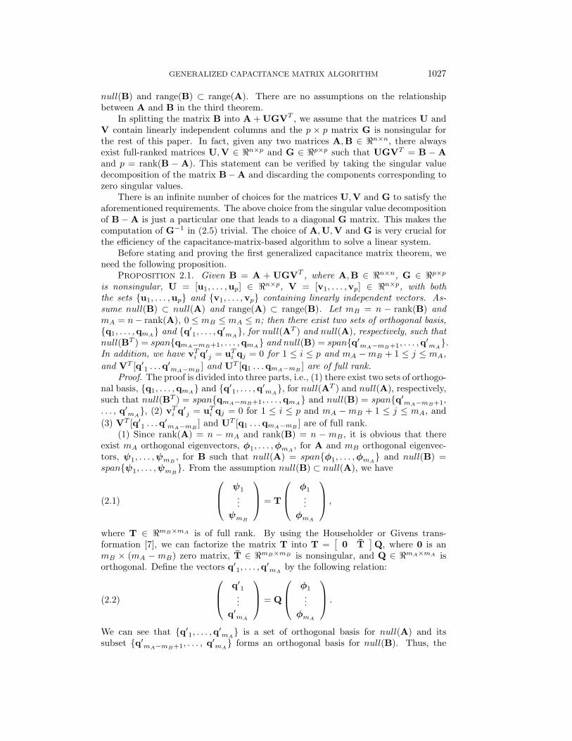
PROPOSITION 2.1. Given B = A + UGVT , where A,B ∈ <n×n, G ∈ <p×pis nonsingular, U = [u1, . . . ,up] ∈ <n×p, V = [v1, . . . ,vp] ∈ <n×p, with boththe sets u1, . . . ,up and v1, . . . ,vp containing linearly independent vectors. As-sume null(B) ⊂ null(A) and range(A) ⊂ range(B). Let mB = n − rank(B) andmA = n− rank(A), 0 ≤ mB ≤ mA ≤ n; then there exist two sets of orthogonal basis,q1, . . . ,qmA and q′1, . . . ,q′mA, for null(AT ) and null(A), respectively, such thatnull(BT ) = spanqmA−mB+1, . . . ,qmA and null(B) = spanq′mA−mB+1, . . . ,q

′mA.

In addition, we have vTi q′j = uTi qj = 0 for 1 ≤ i ≤ p and mA −mB + 1 ≤ j ≤ mA,and VT [q′1 . . .q′mA−mB ] and UT [q1 . . .qmA−mB ] are of full rank.

Proof. The proof is divided into three parts, i.e., (1) there exist two sets of orthogo-nal basis, q1, . . . ,qmA and q′1, . . . ,q′mA, for null(AT ) and null(A), respectively,such that null(BT ) = spanqmA−mB+1, . . . ,qmA and null(B) = spanq′mA−mB+1,. . . , q′mA, (2) vTi q′j = uTi qj = 0 for 1 ≤ i ≤ p and mA −mB + 1 ≤ j ≤ mA, and(3) VT [q′1 . . .q′mA−mB ] and UT [q1 . . .qmA−mB ] are of full rank.

(1) Since rank(A) = n − mA and rank(B) = n − mB , it is obvious that thereexist mA orthogonal eigenvectors, φ1, . . . ,φmA , for A and mB orthogonal eigenvec-tors, ψ1, . . . ,ψmB , for B such that null(A) = spanφ1, . . . ,φmA and null(B) =spanψ1, . . . ,ψmB. From the assumption null(B) ⊂ null(A), we have ψ1

...ψmB

= T

φ1...

φmA

,(2.1)

where T ∈ <mB×mA is of full rank. By using the Householder or Givens trans-formation [7], we can factorize the matrix T into T =

[0 T

]Q, where 0 is an

mB × (mA − mB) zero matrix, T ∈ <mB×mB is nonsingular, and Q ∈ <mA×mA isorthogonal. Define the vectors q′1, . . . ,q

′mA by the following relation: q′1

...q′mA

= Q

φ1...

φmA

.(2.2)

We can see that q′1, . . . ,q′mA is a set of orthogonal basis for null(A) and itssubset q′mA−mB+1, . . . , q′mA forms an orthogonal basis for null(B). Thus, the


existence of the basis q′1, . . . ,q′mA which satisfies the aforementioned requirementsis proved. Similarly, we can prove that there exists an orthogonal basis q1, . . . ,qmAfor null(AT ) and null(BT ) = spanqmA−mB+1, . . . ,qmA is satisfied.

(2) From the assumption, we have Bq′j = Aq′j = 0, mA −mB + 1 ≤ j ≤ mA.Since Bq′j = (A + UGVT )q′j , we have UGVTq′j = 0 for mA −mB + 1 ≤ j ≤ mA.From the assumption that U ∈ <n×p, p ≤ n, has full rank and G is nonsingular,it is obvious that VTq′j = 0. Therefore, we have vTi q′j = 0 for 1 ≤ i ≤ p andmA − mB + 1 ≤ j ≤ mA. Similarly, we can show that uTi qj = 0, 1 ≤ i ≤ p, andmA −mB + 1 ≤ j ≤ mA.

(3) We use proof by contradiction to show that the matrix VT [q′1 . . .q′mA−mB ]is of full rank. Let’s assume this matrix is rank deficient, i.e., there exists a nonzerovector aT = (a1, . . . , amA−mB ) such that VT [q′1 . . .q′mA−mB ]a = 0. Let a vector r be[q′1 . . .q′mA−mB ]a; then r ∈ null(A) and r is orthogonal to null(B). Post-multiplyingboth sides of the equation B = A + UGVT by r yields Br = Ar + UGVT r. SinceAr = 0 and VT r = 0, we obtain Br = 0. But, from the above, r is a nonzerovector orthogonal to null(B), i.e., Br 6= 0, leading to a contradiction. Consequently,the assumption that VT [q′1 . . .q′mA−mB ] is rank deficient is not true, implying thatVT [q′1 . . .q′mA−mB ] is of full rank. Similarly, we can prove that UT [q1 . . .qmA−mB ]is of full rank.

All of the assumptions in Proposition 2.1 will be applied to the first generalizedcapacitance matrix theorem. In addition, we will include the assumption that qTi uj =αiδ(i, j), 1 ≤ i, j ≤ mA −mB , in the theorem in order to compute the projection ofa vector onto the space null(AT ) \ null(BT ), through the vectors u1, . . . ,umA−mB .This assumption can be verified as follows. If U,G,V satisfies UGVT = B −A and each is of full rank, then the alternative set UQ,Q−1G,V also satisfiesthese requirements when the matrix Q ∈ <p×p is nonsingular. From Proposition 2.1,UT [q1 . . .qmA−mB ] has full rank. We can find a transformation matrix Q to make theupper (mA−mB)×(mA−mB) block of the transformed matrix QTUT [q1 . . .qmA−mB ]diagonal. Then, the condition qTi uj = αiδ(i, j), 1 ≤ i, j ≤ mA −mB , is satisfied.

We are now ready to state and prove the first generalized capacitance matrixtheorem.

THEOREM 2.2. Given B = A + UGVT , where A,B ∈ <n×n, G ∈ <p×p isnonsingular, U, V ∈ <n×p, and all the assumptions of Proposition 2.1. Let qTi uj =αiδ(i, j), αi 6= 0 for 1 ≤ i, j ≤ mA −mB.

Let x be a solution to

Ax = b−mA−mB∑j=1

qTj b

qTj ujuj ,(2.3)

where b ∈ range(B). For 1 ≤ i ≤ p, let ηi be a solution to

Aηi = ui −mA−mB∑j=1

qTj uiqTj uj

uj .(2.4)

Define the capacitance matrix C as

C = G−1 + VTη −mA−mB∑j=1

G−1ejqTj U

qTj uj,(2.5)


where η = [η1, . . . ,ηp], and ej is the jth standard basis vector in <p. From (2.4),η1, . . . ,ηmA−mB can be any vectors in null(A). Let η1, . . . ,ηmA−mB be linearly inde-pendent and the linear combinations of q′1, . . . ,q

′mA−mB . Then there exists a unique

solution β to the capacitance matrix equation

Cβ = VT x−mA−mB∑j=1

qTj b

qTj ujG−1ej ,(2.6)

and x− ηβ is a solution to the linear system Bx = b.Proof. The proof is in three parts, and we will show that (1) there exist solutions

to (2.3) and (2.4), (2) the capacitance matrix C is nonsingular, implying that (2.6)has a unique solution, and (3) B(x− ηβ) = b.

(1) By using the fact that uTi qj = 0 for 1 ≤ i ≤ p and mA −mB + 1 ≤ j ≤ mA

from Proposition 2.1 and the assumption b ∈ range(B), we can prove that the RHSsof (2.3) and (2.4) are orthogonal to null(AT ). Consequently, these RHSs are in therange of A, which means there always exist solutions to (2.3) and (2.4).

(2) To prove that C is nonsingular, we show that Cβ = 0⇒ β = 0. Let’s supposeCβ = 0; then, from (2.5), we have

VTηβ =mA−mB∑j=1

G−1ejqTj Uβ

qTj uj−G−1β.(2.7)

By definition, Bηβ = Aηβ+UVTηβ. Substituting (2.4) and (2.7) into this equation,we get Bηβ = 0. Thus, ηβ ∈ null(B). Since null(B) ⊂ null(A), we have ηβ ∈null(A), i.e., Aηβ = 0. Denote β by (β1, . . . , βp). Substituting Aη by (2.4) andrearranging the equation, we obtain

mA−mB∑j=1

(βj −

qTj Uβ

qTj uj

)uj +

p∑j=mA−mB+1

βjuj = 0.(2.8)

Since u1, . . . ,up are linearly independent, (2.8) implies the following conditions onβj :

βj =qTj Uβ

qTj uj, j = 1, . . . ,mA −mB ,(2.9)

βj = 0, j = mA −mB + 1, . . . , p.(2.10)

Substituting these conditions into the RHS of (2.7), we obtain

VT [η1, . . . ,ηmA−mB ]

β1...

βmA−mB

= 0.(2.11)

For i = 1, . . . ,mA −mB , the RHS in (2.4) vanishes, thus ηi ∈ null(A). From the as-sumption that η1, . . . ,ηmA−mB are chosen to be linear combinations of q′1, . . . ,q

′mA−mB

and linearly independent, we have

[η1 . . . ηmA−mB ] = [q′1 . . . q′mA−mB ]T,(2.12)


where T ∈ <(mA−mB)×(mA−mB) is nonsingular. By substituting (2.12) into (2.11), weget

VT [q′1 . . . q′mA−mB ]T

β1...

βmA−mB

= 0.(2.13)

Since VT [q′1 . . . q′mA−mB ] is of full rank and is of size p × (mA − mB) withp ≥ mA − mB proved in Proposition 2.1 and that T is nonsingular, this makesβi = 0, i = 1, . . . ,mA − mB . Combining this with (2.10), we obtain β = 0. Thus,concluding that Cβ = 0 implies β = 0, therefore, C is nonsingular.

(3) Now, we will show that B(x− ηβ) = b. Substituting A + UGVT for B andexpanding, we have

B(x− ηβ) = Ax−Aηβ + UGVT x−UGVTηβ.(2.14)

Rewriting VTηβ using (2.5) and (2.6) and some algebraic manipulation, we get

VTηβ = VT x−mA−mB∑j=1

qTj b

qTj ujG−1ej −G−1β +

mA−mB∑j=1

G−1ejqTj U

qTj ujβ.(2.15)

Substituting for Ax, Aη, and VTηβ from (2.3), (2.4), and (2.15), respectively, (2.14)leads to B(x− ηβ) = b.

Now, let’s turn to the other case when null(A) ⊂ null(B) and range(B) ⊂range(A). Note that several generalized inverse formulas of (A + UGVT ) were givenin [9] under the same constraints. Although these generalized inverse formulas can bedirectly used to solve the linear system with the matrix (A + UGVT ), they happento be special cases of our Theorem 2.4. The multiplication of a generalized inversewith a vector implies the minimum norm solution for the linear system. Therefore, thegeneralized inverse formulas require the minimum norm solutions to the associatedlinear systems, including those with the matrix A and the capacitance matrix. Incontrast, our Theorem 2.4 is valid for any solution to the associated linear systems,thus it is more general than the generalized inverse results.

Before giving the generalized capacitance matrix theorem for this case, we statethe following proposition which is needed in the proof of this theorem.

PROPOSITION 2.3. Given B = A + UGVT , where A,B ∈ <n×n, G ∈ <p×pis nonsingular, U = [u1, . . . ,up] ∈ <n×p, V = [v1, . . . ,vp] ∈ <n×p, with both thesets u1, . . . ,up and v1, . . . ,vp containing linearly independent vectors. Assumenull(A) ⊂ null(B) and range(B) ⊂ range(A). Let q1, . . . ,qmA and q′1, . . . ,q′mAbe the sets of orthogonal eigenvectors in null(AT ) and null(A), respectively, wheremA = n− rank(A). Then, qTi uj = q′Ti vj = 0 for i = 1, . . . ,mA and j = 1, . . . , p.

Proof. From the assumption that null(A) ⊂ null(B), we can see that the eigen-vectors q′i, i = 1, . . . ,mA, are also in null(B). Since Bq′i = Aq′i + UGVTq′i, weobtain

UGVTq′i = 0(2.16)

for 1 ≤ i ≤ mA. The matrix U is of size n× p, n ≥ p, and of full rank, consequently,GVTq′i = 0. From the assumption that G is nonsingular, we have VTq′i = 0.Therefore, q′Ti vj = 0 for i = 1, . . . ,mA and j = 1, . . . , p. Similarly, we can prove thatqTi uj = 0, i = 1, . . . ,mA and j = 1, . . . , p.


THEOREM 2.4. Given B = A + UGVT , where A,B ∈ <n×n, G ∈ <p×p isnonsingular, U and V ∈ <n×p and all the assumptions of Proposition 2.3. Let x bea solution to

Ax = b,(2.17)


Aηi = ui.(2.18)

Define the capacitance matrix C as G−1 + VTη, where η = [η1, . . . ,ηp]. Then thereexists a solution β to the capacitance matrix equation

Cβ = VT x,(2.19)

and x− ηβ is a solution to the linear system Bx = b.Proof. The proof is presented in three parts, namely, (1) we will show that there

exist solutions for (2.17) and (2.18), (2) we will establish that there exists a solutionfor (2.19), and (3) we will show that B(x− ηβ) = b.

(1) To show that there exists a solution for (2.17) and (2.18), we prove that theRHSs of both equations are in the range of A. It is obvious that b ∈ range(A) for(2.17), since b ∈ range(B) and range(B) ⊂ range(A). For (2.18), from Proposition 2.3we can see that ui, 1 ≤ i ≤ p, is orthogonal to null(AT ), which means ui ∈ range(A)for i = 1, . . . , p.

(2) To show that there exists a solution to (2.19), we need to show that VT x isin the range of C. We will use proof by contradiction in the following. Assume thatVT x is not in the range of C; then there exists a nonzero vector γ ∈ null(CT ), i.e.,CTγ = 0, such that

γT (VT x) 6= 0.(2.20)

Using the generalized inverse1 A+ of the matrix A, we can write x as follows:

x = A+b +mA∑i=1

aiq′i,(2.21)

where mA = n − rank(A), q′1, . . . ,q′mA are the orthogonal eigenvectors in null(A),

and ai ∈ < ∀i. Then,

VT x = VTA+b +mA∑i=1

aiVTq′i.(2.22)

From Proposition 2.3, we have VTq′i = 0 for i = 1, . . . ,mA. Substituting into (2.22),we have VT x = VTA+b. Substituting for VT x in (2.20) yields

(A+TVγ)Tb 6= 0.(2.23)

1Let the singular value decomposition of A be A = UΣVT , where U and V are orthogonalmatrices and Σ = diag(0, . . . , 0, λmA+1, . . . , λn). Then its generalized inverse A+ = VΣ+UT ,where Σ+ = diag(0, . . . , 0, 1

λmA+1, . . . , 1

λn) [7].


We can show that A+TVγ ∈ null(BT ) as follows:

BT (A+TVγ) = (A + UGVT )TA+TVγ(2.24)

= (ATA+TV + VGTUTA+TV)γ.(2.25)

Since ATA+T = I−∑mAi=1 q′iq

′Ti , using a result of Proposition 2.3, namely, q′Ti V = 0

for i = 1, . . . ,mA, we have

ATA+TV = V −mA∑i=1

q′iq′Ti V = V.(2.26)

Substituting (2.26) into (2.25) yields

BT (A+TVγ) = VGT (G−1 + VTA+U)Tγ.(2.27)

Again, using Proposition 2.3, we can show that C = G−1 + VTA+U. Consequently,we obtain BT (A+TVγ) = VGTCTγ = 0 since CTγ = 0 by assumption. Thus,A+TVγ ∈ null(BT ). Combining this with (2.23) leads to the conclusion that b isnot in range(B). This is a contradiction to the assumption b ∈ range(B). Therefore,the assumption that VT x is not in the range of C is untrue. Hence, we can concludethat VT x ∈ C. This proves that there exists a solution to (2.19).

(3) The proof for B(x − ηβ) = b is very similar to part (3) of the proof forTheorem 2.2 and is omitted here.

If we restrict the above constraints on the relation between B and A to null(B) =null(A) and range(B) = range(A), then the capacitance matrix C is nonsingular, i.e.,the capacitance matrix equation has a unique solution. This result is stated in thefollowing corollary.

COROLLARY 2.5. In Theorem 2.4, if null(A) = null(B) and range(A) = range(B),then the capacitance matrix C is nonsingular.

Proof. To prove that C is nonsingular, we show that Cβ = 0 ⇒ β = 0. SupposeCβ = 0; then, from the definition of C, we have VTηβ = −G−1β, which can besubstituted into the equation Bηβ = Aηβ+UVTηβ, along with the equation for Aηfrom (2.18), to get Bηβ = 0, i.e., ηβ ∈ null(B). Since null(A) = null(B), we haveAηβ = 0. Using (2.18) for Aη, we get Uβ = 0. From the assumption on the matrixU, namely, u1, . . . ,up are linearly independent, we conclude that β = 0. Therefore,C is nonsingular.

In the above theorems, we impose the constraints on the relationship betweenB and A either via null(B) ⊂ null(A) and range(A) ⊂ range(B) or via null(A) ⊂null(B) and range(B) ⊂ range(A). Now, we consider the general case, i.e., there isno constraint on the relationship between B and A. The following theorem is givenfor this general case and can be used for any matrices B and A in <n×n as long asthere exists a solution for the associated capacitance matrix equation.

THEOREM 2.6. Given B = A + UGVT , where B,A ∈ <n×n, G ∈ <p×pis nonsingular, U = [u1, . . . ,up] ∈ <n×p, V = [v1, . . . ,vp] ∈ <n×p, with boththe sets u1, . . . ,up and v1, . . . ,vp containing linearly independent vectors. LetmA = rank(A) = n −mA, m

′ = dim(null(B) ∩ null(A)), and m = dim(null(BT ) ∩null(AT )), 0 ≤ m′,m ≤ mA ≤ n; then there exist two sets of orthogonal basis,q1, . . . ,qmA and q′1, . . . ,q′mA, for null(AT ) and null(A), respectively, suchthat null(BT ) ∩ null(AT ) = spanqmA−m+1, . . . ,qmA and null(B) ∩ null(A) =


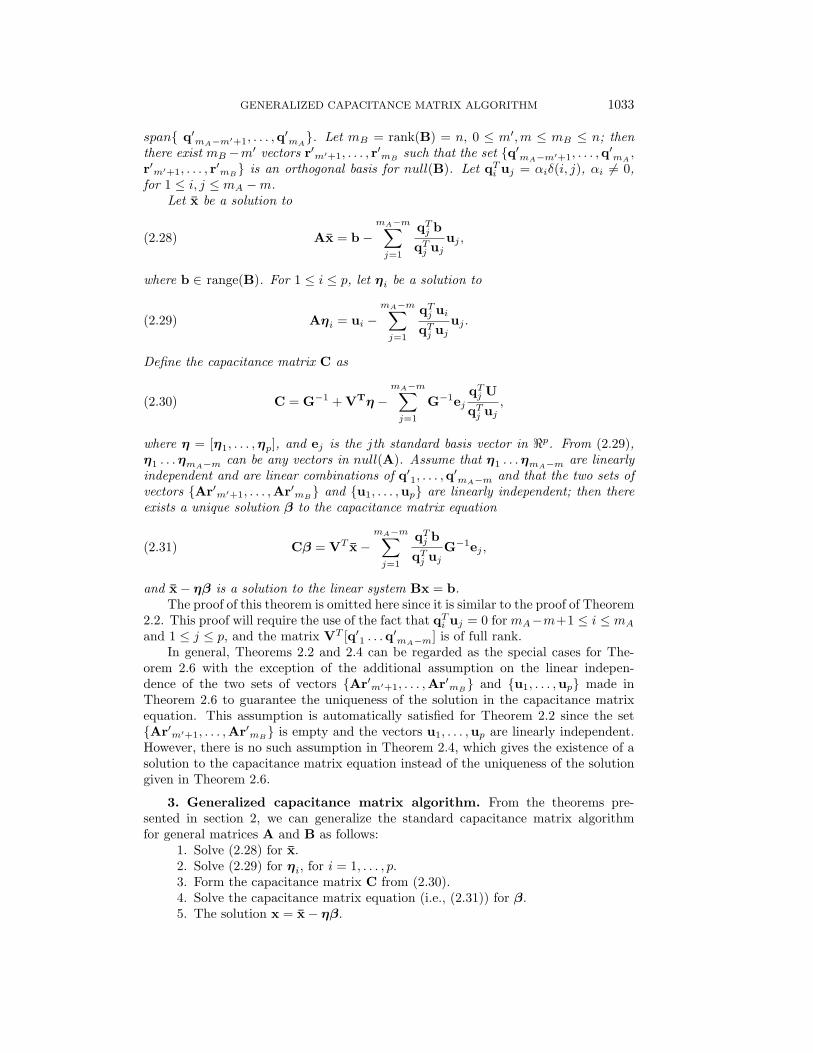
span q′mA−m′+1, . . . ,q′mA. Let mB = rank(B) = n, 0 ≤ m′,m ≤ mB ≤ n; then

there exist mB−m′ vectors r′m′+1, . . . , r′mB such that the set q′mA−m′+1, . . . ,q′mA ,

r′m′+1, . . . , r′mB is an orthogonal basis for null(B). Let qTi uj = αiδ(i, j), αi 6= 0,for 1 ≤ i, j ≤ mA −m.

Let x be a solution to

Ax = b−mA−m∑j=1

qTj b

qTj ujuj ,(2.28)


Aηi = ui −mA−m∑j=1

qTj uiqTj uj

uj .(2.29)

Define the capacitance matrix C as

C = G−1 + VTη −mA−m∑j=1

G−1ejqTj U

qTj uj,(2.30)

where η = [η1, . . . ,ηp], and ej is the jth standard basis vector in <p. From (2.29),η1 . . .ηmA−m can be any vectors in null(A). Assume that η1 . . .ηmA−m are linearlyindependent and are linear combinations of q′1, . . . ,q

′mA−m and that the two sets of

vectors Ar′m′+1, . . . ,Ar′mB and u1, . . . ,up are linearly independent; then thereexists a unique solution β to the capacitance matrix equation

Cβ = VT x−mA−m∑j=1

qTj b

qTj ujG−1ej ,(2.31)

and x− ηβ is a solution to the linear system Bx = b.The proof of this theorem is omitted here since it is similar to the proof of Theorem

2.2. This proof will require the use of the fact that qTi uj = 0 for mA−m+1 ≤ i ≤ mA

and 1 ≤ j ≤ p, and the matrix VT [q′1 . . .q′mA−m] is of full rank.In general, Theorems 2.2 and 2.4 can be regarded as the special cases for The-

orem 2.6 with the exception of the additional assumption on the linear indepen-dence of the two sets of vectors Ar′m′+1, . . . ,Ar′mB and u1, . . . ,up made inTheorem 2.6 to guarantee the uniqueness of the solution in the capacitance matrixequation. This assumption is automatically satisfied for Theorem 2.2 since the setAr′m′+1, . . . ,Ar′mB is empty and the vectors u1, . . . ,up are linearly independent.However, there is no such assumption in Theorem 2.4, which gives the existence of asolution to the capacitance matrix equation instead of the uniqueness of the solutiongiven in Theorem 2.6.

3. Generalized capacitance matrix algorithm. From the theorems pre-sented in section 2, we can generalize the standard capacitance matrix algorithmfor general matrices A and B as follows:

1. Solve (2.28) for x.2. Solve (2.29) for ηi, for i = 1, . . . , p.3. Form the capacitance matrix C from (2.30).4. Solve the capacitance matrix equation (i.e., (2.31)) for β.5. The solution x = x− ηβ.


This generalized capacitance matrix algorithm can always be applied to the caseswhen null(B) ⊂ null(A) and range(A) ⊂ range(B) or when null(A) ⊂ null(B) andrange(B) ⊂ range(A), as stated in Theorems 2.2 and 2.4, respectively. However, toapply this algorithm to more general cases, we need to make sure that a solutionexists to the capacitance matrix equation in step 4. Theorem 2.6 gives a sufficientcondition for the uniqueness of the solution to the capacitance matrix equation in thegeneral case.

Note that step 2 of the algorithm requires the solutions η1, . . . ,ηp in (2.29) withdifferent RHSs. The computational cost to solve this equation p times is very highwhen p is large. However, the vectors η1, . . . ,ηp can be easily obtained when thematrix A is chosen to be circulant Toeplitz and the vectors ui have a very sparse setof nonzero entries. The circulant Toeplitz property of the matrix A makes it shift-invariant, which means AS(u) = S(Au) for all u ∈ <n, where S is a shift operator[13]. A linear shift-invariant operator can be completely characterized by its impulseresponse, which is the solution of the corresponding linear system Au = e, where theRHS e is a unit vector. Thus, the solution ηi can be obtained via the convolution of theimpulse response for this shift-invariant linear system with the RHS in (2.29), whichis sparse since the vectors u1, . . . ,up themselves are sparse. The convolution of theimpulse response with a sparse vector can be easily obtained by a linear combinationof the shifted impulse response vectors. When the vectors vi, i = 1, . . . , p, are alsosparse, the computation of the matrix VTη for forming the capacitance matrix C canbe further simplified by obtaining the (i, j)th entry of VTη from the impulse responsecorresponding to the relative locations of the nonzero components of vi and those ofu1, . . . ,umA−m and uj .

The direct computation of ηβ in the final step of the generalized capacitancematrix algorithm requires O(pn) operations, which are very costly when p, the rankof difference between B and A, is large. Instead, we solve the following linear system

Ay = Uβ −mA−m∑j=1

qTj Uβ

qTj ujuj(3.1)

to get the solution y which has the same projection on the range of A as ηβ. As forthe projection of ηβ on the null space of A, it can be easily computed from the innerproduct of β and ai = (ai,1, . . . , ai,p), where ai,j = qTi ηj , for 1 ≤ i ≤ mA −m. Thecoefficients ai can be chosen arbitrarily as long as the assumption that η1 . . .ηmA−mare linearly independent and are linear combinations of q′1, . . . ,q

′mA−m is satisfied.

Thus, ηβ can be obtained from the following equation:

ηβ = y +mA−m∑i=1

(aTi β −

qTi yqTi qi

)qi.(3.2)

The flowchart of the generalized capacitance matrix algorithm is given in Fig. 3.1.This algorithm relies on an efficient solver for the linear system with the matrix A.The choice of A is very crucial for the efficiency of the algorithm. In addition to thesolution for the linear system with the matrix A, the solution to the linear systemwith the capacitance matrix is also very critical to the efficiency of the generalizedcapacitance matrix algorithm. Since the size of the capacitance matrix is equal to therank of B−A, another criteria for choosing the matrix A is that the rank of B−Ais small. We only give very general description for the generalized capacitance matrixalgorithm in this section. It is not practical to obtain the computational complexity


b

Input data Split B into A + UGV T

x

x - ηβCompute

x

C

β

η i

ηβ

compute ηβ from (3.2)

Solve (2.28) for Solve (2.29) for

Solve (3.1) for y &

Solve capacitance matrix

Form the capacitancematrix C from (2.30)

eq. in (2.31) for β

FIG. 3.1. The flow chart of the generalized capacitance matrix algorithm.

for the generalized capacitance matrix algorithm on general problems. In fact, thealgorithms for solving the linear systems with the matrix A and the capacitancematrix C should exploit the structure of the problem in order to achieve the bestefficiency. We will dwell on the specific numerical algorithms for solving the linearsystems and their computational complexities for some computer vision problems inthe next section.

4. Applications to computer vision. We have successfully applied our gen-eralized capacitance matrix algorithm to a host of computer vision problems which usethe membrane and/or thin-plate spline to constrain the solution [23, 11]. These com-puter vision problems include the surface reconstruction, shape from shading, opticalflow computation, lightness problem, etc. [23, 11]. These problems, when formulatedas variational principles and discretized, lead to solving one or more large sparse linearsystems. In this paper, we present the application of our generalized capacitance ma-trix algorithm to some computer vision problems, namely, the surface reconstructionproblem, the surface interpolation problem, and the shape from orientation problem.

4.1. The surface reconstruction problem. The surface reconstruction prob-lem involves approximating a set of depth or elevation values with a piecewise smoothsurface. Surface reconstruction/recovery from range/depth data has been intenselyresearched for the past decade by many researchers in the computer vision community[1, 22, 2, 24, 23]. Variational splines [22] have emerged as the single most popularsolution to the surface reconstruction problem. In the following, we give the preciseexpressions for the smoothness and data constraints used in the variational formula-tion of surface reconstruction problem. The smoothness constraint involving only thefirst-order derivative terms can be written as [22],

Es(v) =∫ ∫

Ω(v2x + v2

y)dxdy,(4.1)


where v(x, y) is the admissible function [22], vx, vy are its partial derivatives, and Ωis a rectangular domain over which the data (to be approximated) is specified.

The above energy expression can be interpreted as the deflection energy in amembrane (e.g., a rubber sheet) and serves as a stabilizer in the overall variationalprinciple for the surface reconstruction problem. Equation (4.1) is popularly known asthe membrane stabilizer in computational vision literature. Another popular stabilizerin computational vision is the thin-plate stabilizer, which enforces the smoothness ofthe first-order derivatives. The thin-plate stabilizer can be obtained by replacingthe integrand in (4.1) by (vxx)2 + 2(vxy)2 + (vyy)2. For ease of exposition, we willconcentrate on the membrane stabilizer for the rest of this paper.

To the stabilizer we add data constraints via what are known as penalty terms.The following penalty term which measures the discrepancy between the surface anddata weighted by the uncertainty in the data may be used [22]:

Ed(v) =12

∑ci (v(xi, yi)− di)2

,(4.2)

where di are the depth data points specified over a sparse set of locations in thedomain Ω and ci are the uncertainties associated with the data. The total energyis E(v) = λEs(v) + Ed(v), where λ is the regularization parameter that controls theamount of smoothing performed. The goal is to find a v∗ that minimizes the totalpotential energy E(v). (For more details, see [22].)

To compute a numerical solution to the above minimization problem, we firstdiscretized the functionals Es(v) and Ed(v) using the finite element technique [22],which uses the linear triangular element on the rectangular domain Ω. The energydue to the data compatibility term in discrete form becomes

Ed(x) =12

(x− d)TKd(x− d),(4.3)

where x ∈ <n is the concatenation of the n nodal variables vij on a (m×m) mesh forthe discretized surface, d ∈ <n contains the data points, and Kd ∈ <n×n is a diagonalmatrix (for uncorrelated noise in the data) containing the uncertainties σi associatedwith the data points. The smoothness energy in discrete form is

Es(x) =12xTKsx,(4.4)

where Ks ∈ <n×n is a large, sparse, and block-banded matrix called the stiffnessmatrix. The resulting energy function E(x) = λEs(x) + Ed(x) is a quadratic in xgiven by

E(x) =12xTBx− xTb + c(4.5)

with B = λKs + Kd and b = Kdd. The minimum E(x∗) of this energy function isfound by solving the large sparse linear system Bx = b. The structure of the stiffnessmatrix B can be analyzed using the computational molecules as defined in [22].

Several numerical algorithms have been used to solve this linear system, includ-ing the conjugate gradient algorithm, the hierarchical basis preconditioned conjugategradient algorithm [20], and the multigrid relaxation algorithm [21]. The conjugategradient algorithm takes O(n2) operations. Although the hierarchical basis conju-gate gradient was proved to take O(n log n) operations for solving the linear system


discretized from the second-order elliptic boundary value problem [25], there is no the-oretical result on its computational complexity for the surface reconstruction problem.The multigrid relaxation algorithm can solve the Poisson equation in O(n) operations[3]; however, the construction of the multigrid becomes very involved for irregulardomain. In addition, no similar computational complexity result has been proved forthe surface reconstruction problem.

Before applying our generalized capacitance matrix algorithm to solve the largesparse linear system Bx = b, we have to carefully choose the matrix A for splitting Binto A + UVT to make the resulting algorithm efficient. There are three criteria thatdictate the choice A. The first is that the difference between B and A must be smallin the sense that rank(B−A) is small. Second, A must possess some nice structure soas to have a fast numerical solution for the associated linear system. Last, A shouldbe circulant Toeplitz; this property has the advantage of saving the computationalcost in solving (2.29) for each ηi, 1 ≤ i ≤ p, when the corresponding RHSs are verysparse. Taking into consideration the three criteria given above, we can choose A asthe discrete Laplacian operator on the doubly periodic embedded rectangular domain.The exact form of A is given by

A =

D −I −I

−I. . . . . .. . . . . . . . .

. . . . . . −I−I −I D

,(4.6)

where

D =

4 −1 −1−1 4 −1

. . . . . . . . .−1 4 −1

−1 −1 4

.(4.7)

The matrix A can be regarded as the 5-point approximation of the Laplacianoperator on a doubly periodic embedded rectangular domain. From a computationalmolecule [22] point of view, only the membrane molecule is used at every node ofthe doubly periodic rectangular domain. Therefore, the data constraint molecule,derivative (Neumann boundary) constraint molecule, and all molecular inhibitionsdue to depth discontinuities and the imposed doubly periodic boundary condition areincluded in the matrix UVT . Since UVT =

∑pi=1 uivTi , each uivTi can be considered

as a data constraint molecule, a derivative constraint molecule, or a molecule inhi-bition at some location. Thus, we can see that the structures of ui and vi are verysimple. Each vector contains either one or two nonzero components. One nonzerocomponent is for the case of the data constraint molecule while two nonzero compo-nents are for the other two cases.

Note that the generalized inverse forms of (A + UVT ) presented in [18] and [9]cannot be applied to the above problem because of the restrictive assumptions im-posed on matrices A and B. With the above choice of A, the dimension of the nullspace of A is one and the rank of UVT is the number of data constraints and all molec-ular inhibitions due to depth discontinuities as well as the imposed doubly periodic


boundary condition. Consequently, the assumption rank(UVT ) ≤ dim(null(A))(= 1)implied by Riedel’s result [18] is violated. The generalized inverse forms presentedin [9] are valid only when range(B) ⊂ range(A) and both the matrices A and B aresymmetric. In this case, the matrix B is nonsingular and rank(A) = n− 1, thereforethe assumption range(B) ⊂ range(A) in [9] is violated.

We can see that this particular choice of A makes it circulant Toeplitz and thustranslation invariant. In addition, it can be decomposed as the sum of two tensorproducts of matrices A and I, i.e.,

A = A⊗ I + I⊗ A,(4.8)

with

A =

2 −1 −1−1 2 −1

. . . . . . . . .−1 2 −1

−1 −1 2

∈ <m×m,

and ⊗ denotes the tensor (Kronecker) product. By using this special structure ofthe matrix A, we can rewrite any linear system of the form Az = f as the followingLyapunov matrix equation:

AZ + ZA = F,(4.9)

where Z and F are m × m matrix representations of the n = m2 vectors z and f ,respectively. It should be noted that the matrix A in (4.9) is circulant Toeplitz andsymmetric positive semidefinite. We can use the ADI method to solve this Lyapunovmatrix equation in O(n) operations [11].

Since the matrix A is chosen to be circulant Toeplitz and there are only oneor two nonzero components in each ui, we can form the capacitance matrix C veryefficiently from the impulse response of the shift-invariant linear system with matrixA and the relative locations between the nonzero components of the vectors vi anduj , as discussed in section 3. To compute the impulse response h of the linear systemAh = e, we can once again use the ADI method to solve the corresponding Lyapunovmatrix equation in O(n) operations.

The linear system with the capacitance matrix C is nonsymmetric. The sizeof the capacitance matrix is determined by the rank of the matrix UVT , which isdependent on the total number of data constraints and molecular inhibitions dueto depth discontinuities and the imbedding of the doubly periodic boundary. Weuse the biconjugate gradient (BCG) method to solve this linear system. The BCGmethod involves the matrix–vector multiplication in each iteration, which takes O(p2)operations. The BCG converges to the solution in at most p iterations; however, thisconvergence can be speeded up with appropriate preconditioning.

Proskurowski and Vassilevski [15] reviewed several different preconditioners forthe capacitance matrix arising from the second-order elliptic partial differential equa-tion. Among them, Dryja’s preconditioner [6] based on the square root of the finitedifference analogue of −(d2/ds2) along the boundary was proved to be spectrallyequivalent to the capacitance matrix, which means that a conjugate-gradient-typealgorithm applied to solve this linear system can converge in a constant number ofiterations. The hierarchical basis preconditioner [19] has been proved to reduce the


(a) (b)

(c) (d)

(e) (f)

FIG. 4.1. Surface reconstruction example: (a) original sparse data, (b) interpolating surfaceobtained using the generalized capacitance matrix algorithm; (c) the same sparse data set with depthdiscontinuities along the indicated horizontal line, (d) reconstructed surface; (e) the same sparsedata set with depth discontinuities along the indicated diagonal line, (f) reconstructed surface.

condition number of the transformed capacitance matrix to O(log2 n). Although thesepreconditioners cannot be directly applied to the surface reconstruction problem, itis possible to use a similar construction procedure. Such a preconditioner will speedup the convergence of the BCG algorithm for solving the capacitance matrix linearsystem. A discussion on preconditioning the capacitance matrix is out of the scope ofthis paper and will be the focus of our future research.

We implemented our generalized capacitance matrix algorithm on the sparsedata surface reconstruction with membrane smoothness constraint. We synthesized asparse range/elevation data set on a 64 × 64 grid. The input data set is very sparseand contains 15 data points randomly scattered in the plane as shown in Fig. 4.1a.We apply our algorithm to this data to obtain a smooth surface approximation. Inthis example we observe that only 10 ADI iterations are needed to attain an errortolerance of 10−5. We depict the surface obtained using our generalized capacitance


matrix algorithm with 10 ADI iterations for solving the linear systems with matrixA in Fig. 4.1b. We also apply our generalized capacitance matrix algorithm for thesame data set with depth discontinuities. In Fig. 4.1c, the depth discontinuities alongthe line between coordinates (1, 32) and (30, 32) are introduced. The reconstructedsurface using our generalized capacitance matrix algorithm is shown in Fig. 4.1d. Asimilar experiment was performed with depth discontinuities along the diagonal linesegment extending from the coordinate (1, 63) to (63, 1). The data along with therecovered surface are shown in Fig. 4.1e and 4.1f, respectively.

Similar choices for the matrix A can be used for other computer vision problemsusing the membrane spline stabilizer. We can choose the well-structured matrix A,which is close to the matrix B, i.e., the stiffness matrix in the large linear system, tobe the Laplacian matrix, thus making the matrix UVT encode the components of thestiffness matrix corresponding to the data constraints, discontinuities, and boundaryconditions. The resulting matrices A and B either satisfy the condition null(B) ⊂null(A) and range(A) ⊂ range(B) in Theorem 2.2 (for surface reconstruction andoptical flow) or satisfy the condition null(A) ⊂ null(B) and range(B) ⊂ range(A)in Theorem 2.4 (for shape from orientation and lightness problem). We refer theinterested reader to [11] for illustrative examples.

4.2. Surface interpolation problem. The surface interpolation problem issimilar to the surface smoothing problem except that the depth/range data constraintsare treated differently. For the surface smoothing problem, the data constraints areused in the data compatibility energy term combined with the smoothness energyterm in the total energy. The minimum energy solution seeks a compromise betweenthe data constraints and the smoothness constraints. Therefore, the data constraintsare “weak” constraints in the surface smoothing problem. On the contrary, the dataconstraints are “hard” constraints in the surface interpolation, i.e., the interpolatedsurface must satisfy the data constraints exactly.

By using the same notation as in section 4.1, the surface interpolation problemcan be formulated as follows: to find a solution v that minimizes the smoothnessenergy functional

S(v) =∫ ∫

Ω(v2x + v2

y)dxdy,(4.10)

under the constraints that

v(xi, yi) = di; (xi, yi) ∈ D ⊂ Ω.(4.11)

Note that the domain Ω is the region of interest, usually assumed to be a rectangularregion for convenience of discretization and computation, and the set D(⊂ Ω) containsthe locations of the data constraints.

The above variational formulation leads to the following Euler–Lagrange equation:

∆v(x, y) = 0 in Ω \D,(4.12)v(xi, yi) = di,(xi, yi) ∈ D.(4.13)

Equation (4.12) is a Laplace equation and D is a set of data locations. It is notnecessarily a standard boundary value problem, whose boundary condition is givenalong a closed contour, since the set D is not a closed contour. We discretize the aboveproblem by using either the finite element method with linear triangular elements[22] or the finite difference method and assume that each data location in the set D


exactly matches a discretization node. This leads to the linear system Kx = b, whereK ∈ <n×n, x and b ∈ <n. The structures of K,x, and b are given by

K =[

K11 K12

0 I

], x =

[x1

x2

], b =

[0d

],(4.14)

where n(= m2) is the number of nodal variables after discretizing the rectangulardomain Ω, K11 ∈ <(n−p)×(n−p), with p being the number of data points, is thestiffness submatrix after discretizing the Laplace equation for the elements insideΩ \D, K12 is the stiffness submatrix after discretizing the Laplace equation for theelements connecting Ω \ D and D, x1 and x2 are vectors consisting of the nodalvariables in Ω \ D and D, respectively, after the discretization, and d is the vectorcontaining the data values di at the locations given in D. For the discretization ofthe Laplacian equation over the entire domain Ω, we can write the stiffness matrix Kas follows:

K =[

K11 K12

K21 K22

]∈ <n×n.(4.15)

Note that the differences between the matrices K and K are in the (2,1) and (2,2)blocks, which are the rows corresponding to the nodal variables at the data locations.These differences can be encoded in the matrix UVT when using the generalizedcapacitance matrix algorithm.

Let’s define a vector x to be a permutation of the nodal variables in the vectorx such that the concatenation of the nodal variables is in a regular order, i.e., rowby row in the discretization mesh. Assume the permuted linear system is Bx = b,where B = PKPT, x = Px, b = Pb, where P is a permutation matrix. Then wecan decompose the matrix B into A + UVT , where A is given in (4.6) and UVT =∑pi=1 uiviT encodes the differences of the rows corresponding to the nodal variables

at the data locations between K and K, and the disabling of the doubly periodicboundary condition imposed on A. In the pair ui,vi, due to the differences betweenthe rows of K and K, the vector ui contains only one nonzero entry 1 at the locationcorresponding to the data point, and the vector vi contains five nonzero entries,namely, four 1’s and one −3, with the entry −3 at the location corresponding to thedata point and the 1’s at the four nearest neighbors of the node at the data point.For the pair ui,vi used in disabling of the doubly periodic boundary condition, wehave ui = −vi with the vector ui containing two nonzero entries 1 and −1. Similarto the surface smoothing, we can include discontinuities into the surface interpolationproblem by using appropriate ui,vi with the structure similar to those used fordisabling the doubly periodic boundary condition.

With the above decomposition of the matrix B into A + UVT , we can apply thegeneralized capacitance matrix algorithm to solve the linear system Bx = b. Onceagain, the ADI method can be used to solve the linear system with the matrix A inO(n) operations [11]. The computational algorithm for the surface interpolation isvery similar to that for the surface smoothing except that the entries in the vectorsui and vi corresponding to the data constraints are different.

Although the generalized capacitance matrix algorithm relies on efficient solvers,such as the ADI method in this paper, for problems with matrix A, the overallefficiency is also dependent on an efficient solution to the capacitance matrix equation.The BCG method is used to solve the linear system with the capacitance matrix, butits computational complexity usually depends on the distribution of data points andthe distribution of discontinuity locations.


Several iterative numerical methods have been used in the past to solve the lin-ear system Bx = b arising in the surface interpolation problem. Their computa-tional complexities are similar to those for solving the surface reconstruction problemdiscussed in the previous section. The conjugate gradient algorithm takes O(n2)operations and the conjugate gradient with hierarchical basis preconditioning takesapproximately O(n log n) [25, 20].

In our solution to this problem, as discussed previously, the ADI method takesO(n) operations and the BCG method converges in at most p iterations, with eachiterations taking O(p2) operations, where p is normally O(m). However, the conver-gence of the BCG method can be improved by using appropriate preconditioning asdiscussed in section 4.1.

When the data points are given along a closed contour and we are interested in thesolution inside the closed contour, the surface interpolation problem becomes a bound-ary value problem. This case is very popular in stereo vision, where the depth data isusually available along the object’s occluding contour. In this case, we discretize theLaplace equation, i.e., (4.12), with the inclusion of doubly periodic boundary condi-tion, which does not influence the solution inside the closed contour. Then the matrixUVT only contains the differences of rows corresponding to the boundary condition,i.e., data constraints, between K and K. Dryja’s spectrally equivalent preconditioner[6] for the capacitance matrix arising from the elliptic boundary value problem can bedirectly applied to this problem, thus making the BCG method converge in a constantnumber of iterations. Thus, our generalized capacitance matrix algorithm can solvethis problem in O(n) operations.

4.3. Shape from orientation problem. The shape from orientation problemis to recover the shape of a surface from the orientation constraints. This problem isa part of the shape from shading problem [10], which involves recovering the shape ofan object from its shaded image. The problem can be formulated as follows: to findthat surface z(x, y) whose partial derivatives zx(x, y) and zy(x, y) are closest to thecomputed gradients denoted by p(x, y) and q(x, y) by minimizing the functional

E(z) =∫ ∫

Ω((zx − p)2 + (zy − q)2) dxdy,(4.16)

where Ω is the region over which the gradients p(x, y) and q(x, y) are computed.The region of the object projected on the image for this problem is typically non-rectangular.

The Euler–Lagrange equation for the above energy functional is a Poisson equa-tion

∆z = px + qy in Ω.(4.17)

For simplicity, we assume there is no boundary condition here. The following algo-rithm can be easily modified to include the boundary conditions.

To solve the above Poisson equation, we first embed the domain Ω into a rectan-gular region R and then discretize the Poisson equation using either the finite elementmethod [22] or the finite difference method on the embedded domain R with the dou-bly periodic boundary condition imposed on ∂R. The imposed periodic boundarycondition has no influence on the solution in Ω. The discretization yields a linearsystem Kx = b, where

K =[

K11 00 K22

]∈ <n×n, x =

[x1

x2

]∈ <n, b =

[d0

]∈ <n,(4.18)


where n(= m2) is the number of nodes after discretization in the embedded domain R,K11 and K22 are stiffness matrices corresponding to the discretized Laplace equationfor elements in Ω and R \ Ω, respectively, x1 and x2 are vectors consisting of thediscretized nodal variables in Ω and R\Ω, respectively, and d is the vector containingthe values from the discretization of px + qy.

Consider the Poisson equation embedded in the domain R with a doubly periodicboundary condition, i.e.,

∆z = f in R,(4.19)

where

f(x, y) =px(x, y) + qy(x, y), (x, y) ∈ Ω,0, (x, y) ∈ R \ Ω.(4.20)

The discretization of the above embedded problem leads to a linear system Kx = b,where

K =[

K11 K12

K21 K22

]∈ <n×n, x =

[x1

x2

]∈ <n, b =

[d0

]∈ <n.(4.21)

Note that the matrix K is a permuted Laplacian matrix. The differences between thematrices K and K are in the (1,2) and (2,1) blocks, which encode the discretizationof the Laplacian operator across the boundary of the region Ω.

The linear system Kx = b can be permuted into a linear system Bx = b toobtain a regular ordering for the nodal variables in x. Similar to section 4.2, we candecompose the matrix B into A+UVT , where A is the Laplacian matrix with doublyperiodic boundary condition. The matrix UVT is used to disable the Laplacianoperator across the boundary of Ω. For each pair ui,vi, we have ui = −vi. Inaddition, there are only two nonzero entries 1 and −1 in each vector ui or vi.

The algorithms to solve the associated linear systems with the matrix A and thecapacitance matrix are similar to that for the surface reconstruction and surface in-terpolation problems. Since the structure of the capacitance matrix is similar to thatof the surface interpolation problem with data points given along a closed contour, wecan apply a preconditioning technique similar to that in [6] to obtain an O(n) solu-tion for the shape from orientation problem. Existing algorithms usually take O(n2)(conjugate gradient) or O(n log n) (hierarchical basis conjugate gradient) operations.

For this problem, we tested our algorithm on a shape from shading example.We use a synthetically generated image of a Lambertian sphere illuminated by adistant point source and viewed from the same location as the point source. Figure4.2a depicts the 64 × 64 original shaded image with an 8 bit resolution, in gray,per pixel. The sphere is assumed to have Lambertian reflectance properties with aconstant albedo. The occluding boundary for the object domain Ω is depicted in Fig.4.2b. The surface orientation is recovered from the shaded image using techniquesdiscussed in [11] and is shown in Fig. 4.2c. The final surface shape obtained usingthe orientation information and applying the above discussed shape from orientationmethod is depicted in Fig. 4.2d.

5. Conclusion. In this paper, we presented the generalized capacitance ma-trix theorems and algorithm for solving linear systems. Our generalized capacitancematrix algorithm can be used for very general matrices A and B, therefore this algo-rithm can be applied to a very broad class of problems and we have ample freedom to


(a) (b)

(c) (d)

FIG. 4.2. Shape from shading example: (a) shaded sphere image, (b) irregular occluding bound-ary embedded in a rectangle, (c) recovered surface orientation, (d) reconstructed surface shape.

choose the matrix A appropriately for designing efficient numerical algorithms. Thetraditional capacitance matrix algorithm [4, 16, 17, 15] has been primarily appliedto solve the second-order elliptic boundary value problems, whereas our generalizedcapacitance matrix algorithm can be used to solve any-order elliptic boundary valueproblems.

Previous work [5, 9, 18] on deriving the generalized inverse forms of (A + UVT )were presented under restrictive assumptions. Although our generalized capacitancematrix theorems are developed for solving general linear systems, it is possible toderive the generalized inverse form of (A + UGVT ) for more general cases based onthese theorems.

We applied the generalized capacitance matrix algorithm to some computer visionproblems, namely, surface reconstruction, surface interpolation, and shape from ori-entation. Although the generalized capacitance matrix algorithm relies on an efficientsolver for the linear system with the matrix A, the solution to the capacitance matrixlinear system is also very important for the efficiency of the entire algorithm. Appro-


priate preconditioning can greatly improve the efficiency for solving the capacitancematrix linear system [15]. The design of such preconditioners for various computervision problems will be the focus of our future research.

REFERENCES

[1] A. BLAKE AND A. ZISSERMAN, Visual Reconstruction, MIT Press, Cambridge, MA, 1987.[2] R. BOLLE AND B. VEMURI, On three-dimensional surface reconstruction methods, IEEE Trans.

Patt. Anal. Mach. Intell., 13 (1991), pp. 1–13.[3] D. BRAESS, The convergence of a multigrid method with Gauss-Seidel relaxation for the Pois-

son equation, Math. Comp., 42 (1984), pp. 505–519.[4] B. L. BUZBEE, F. W. DORR, J. A. GEORGE, AND G. H. GOLUB, The direct solution of the

discrete Poison equation on irregular regions, SIAM J. Numer. Anal., 8 (1971), pp. 722–736.

[5] S. CAMPBELL AND C. MEYER, Generalized Inverses of Linear Transformations, Pitman,Boston, MA, 1979.

[6] M. DRYJA, Capacitance matrix method for Dirichlet problem on polygon region, Numer. Math.,39 (1982), pp. 51–64.

[7] G. H. GOLUB AND C. F. V. LOAN, Matrix Computations, 2nd ed., The Johns Hopkins Univer-sity Press, Baltimore, MD, 1989.

[8] W. W. HAGER, Updating the inverse of a matrix, SIAM Rev., 31 (1989), pp. 221–239.[9] H. V. HENDERSON AND S. R. SEARLE, On deriving the inverse of a sum of matrices, SIAM

Rev., 23 (1981), pp. 53–60.[10] B. K. P. HORN, Height from shading, Internat. J. Comput. Vision, 5 (1990), pp. 174–208.[11] S.-H. LAI AND B. C. VEMURI, An O(N) iterative solution to the Poisson equations in low-

level vision problems, in IEEE Conf. Comp. Vision & Patt. Recog., Seattle, WA, June 1994,pp. 9–14; also Tech. report TR93-035, Department of Computer and Information Sciences,University of Florida, Gainesville, FL, 1993.

[12] D. O’LEARY, A note on the capacitance matrix algorithm, substructuring, and mixed or Neu-mann boundary conditions, Appl. Numer. Math., 3 (1987), pp. 339–345.

[13] A. OPPENHEIM, Discrete-time Signal Processing, Prentice–Hall, Englewood Cliffs, NJ, 1989.[14] D. V. OUELLETTE, Schur complements and statistics, Linear Algebra Appl., 36 (1981), pp. 187–

295.[15] W. PROSKUROWSKI AND P. VASSILEVSKI, Preconditioning capacitance matrix problems in

domain imbedding, SIAM J. Sci. Comput., 15 (1994), pp. 77–88.[16] W. PROSKUROWSKI AND O. WILDLUND, On the numerical solution of Helmholtz’s equation

by the capacitance matrix method, Math. Comp., 30 (1976), pp. 433–468.[17] W. PROSKUROWSKI AND O. WILDLUND, A finite element capacitance matrix method for the

Neumann problem for Laplace’s equation, SIAM J. Sci. Statist. Comput., 1 (1980), pp. 410–425.

[18] K. S. RIEDEL, A Sherman-Morrison-Woodbury identity for rank augmenting matrices withapplication to centering, SIAM J. Matrix Anal. Appl., 13 (1992), pp. 659–662.

[19] B. SMITH AND O. WILDLUND, A domain decomposition algorithm using a hierarchical basis,SIAM J. Sci. Statist. Comput., 11 (1990), pp. 1212–1226.

[20] R. SZELISKI, Fast surface interpolation using hierarchical basis functions, IEEE Trans. Patt.Anal. Machine Intell., 12 (1990), pp. 513–528.

[21] D. TERZOPOULOS, Image analysis using multigrid relaxation methods, IEEE Trans. Patt. Anal.Machine Intell., 8 (1986), pp. 129–139.

[22] D. TERZOPOULOS, The computation of visible-surface representations, IEEE Trans. Patt. Anal.Machine Intell., 10 (1988), pp. 417–438.

[23] B. C. VEMURI AND S.-H. LAI, A fast solution to the surface reconstruction problem, in SPIEConf. on Math. Imaging: Geom. Methods Comp. Vision, San Diego, CA, July 1993, pp. 27–37.

[24] B. C. VEMURI AND R. MALLADI, Constructing intrinsic parameters with active models forinvariant surface reconstruction, IEEE Trans. Patt. Anal. and Machine Intell., 15 (1993),pp. 668–681.

[25] H. YSERENTANT, On multi-level splitting of finite element spaces, Numer. Math., 49 (1986),pp. 379–412.

AND ALGORITHM FOR SOLVING LINEAR SYSTEMSlai/SISC.pdf · ... this method was based on the...

Documents

Transcript of AND ALGORITHM FOR SOLVING LINEAR SYSTEMSlai/SISC.pdf · ... this method was based on the...