
Analyzing the Dependence Structure of Microarray … di Dottorato in Scienze Economiche e...
142
Scuola di Dottorato in Scienze Economiche e Statistiche Dottorato di Ricerca in Metodologia Statistica per la Ricerca Scientifica XX ciclo Alma Mater Studiorum - Universit`a di Bologna Analyzing the Dependence Structure of Microarray Data: a Copula–Based Approach Francesca Marta Lilja Di Lascio Dipartimento di Scienze Statistiche “P. Fortunati” Marzo 2008
-
Upload
vuongkhanh -
Category
Documents
-
view
214 -
download
0
Transcript of Analyzing the Dependence Structure of Microarray … di Dottorato in Scienze Economiche e...

Scuola di Dottorato in Scienze Economiche e Statistiche
Dottorato di Ricerca in
Metodologia Statistica per la Ricerca Scientifica
XX ciclo
Alm
aM
ater
Stu
dio
rum
-U
niv
ersitadiB
olo
gna
Analyzing the Dependence Structure
of Microarray Data:
a Copula–Based Approach
Francesca Marta Lilja Di Lascio
Dipartimento di Scienze Statistiche “P. Fortunati”
Marzo 2008


Scuola di Dottorato in Scienze Economiche e Statistiche
Dottorato di Ricerca in
Metodologia Statistica per la Ricerca Scientifica
XX ciclo
Analyzing the Dependence Structure
of Microarray Data:
a Copula-Based Approach
Fkancesca Marta Lilja Di Lascio
Coordinatore
Prof.ssa Daniela Cocchi
Tutor
Prof-ssa Paola Monari
Co-tutor
Dott. Simone Giannerini
6 &-*"-
Settore Disciplinare
SECS-S/Ol
Dipartimento di Scienze Statistiche "P. Fortunati"
Marzo 2008


To my father.
His thirst for knowledge
will continue to inspire me
for the rest of my life.


Preface
The analysis of microarray data with statistical methods is a topic with important practical
implications. During the last ten years clustering techniques have been largely used in the
first steps of the analysis of microarray data. In literature many algorithms and methods
have been proposed each one with its pros and cons. Many works have demonstrated the
usefulness of clustering biological data even if in literature the clustering of dependent
data, especially in microarray data analysis, has not been through investigated.
The idea of introducing and utilizing the copula functions in a clustering technique
was born during the period I spent at the Department of Biology of the University of
Pennsylvania, Philadelphia, USA during which I worked with Professor Warren J. Ewens.
At the UPENN I had the opportunity of enriching my knowledge of statistical methods for
microarray data analysis and the theory of copula functions which I had previously met
thank to Professor Estela Bee Dagum (during a conference on Time Series Analysis). The
idea and the realization of a simulation study to test the capability of some well–known
clustering methods in correctly finding clusters of dependent data have taken place at the
University of Philadelphia. From this study many interesting limits of classical clustering
methods emerged.
My work continued and ended at the Department of Statistical Science “P. Fortunati”
of the University of Bologna, Italy. Based on such experiences I thought about a new
procedure able to overcome the limits of other clustering techniques investigated. The
work led to a new clustering algorithm based on copula functions. By using criteria based
on maximum likelihood copula function, the proposed algorithm is built to group observa-
tions preserving the underlying dependence structure. The algorithm has been tested on
simulated data and compared with the performance of the model–based clustering tech-
niques in order to evaluate its performance. In light of the satisfactory results obtained I
finally applied it to a real microarray data set.
The use of copulas to investigate the dependence relationship between genes or biolog-
ical samples is thought as a new starting point to enlarge the knowledge of the biological
processes.
Although different people have participated to my dissertation I am responsible for
any errors that may remain.
v

vi Preface
Acknowledgements
Writing a dissertation can be a lonely and isolating experience but it is obviously not
feasible without the personal and practical support of numerous people. First of all, I
would like to express my sincere thanks and appreciation to my supervisor, Prof. Paola
Monari, for guidance and for providing me with excellent facilities to pursue my work.
Second, I am enormously grateful to my co–supervisor, Dr. Simone Giannerini, who made
me a better programmer, followed my work in each of its part making interesting questions
and giving me helpful suggestions. I also thank him for his continued support and frank
comments throughout my research. Third, I thank Prof. Warren J. Ewens for having given
me the possibility to deepen my knowledge of microarray data analysis and for discussions
about it when I was a visiting student at the University of Pennsylvania, Philadelphia,
USA. Last but not least, I thank Prof. Estela Bee Dagum for her comments on this
dissertation and for her precious advices given in the whole my Ph.D. experience.
I also thank Dr. Cinzia Viroli, Prof. Antonella Capitanio and Prof. Rossella Miglio,
all from the University of Bologna, Italy, for their interesting comments and helpful sug-
gestions.
My sincere gratitude goes to my mother and my sister, to their closeness and their
affection. A special thought goes to my father, prematurely passed away, for being lovely
interested in my Ph.D. experience, for having taught me the love for study and research
and advised me to get into the fabulous world of research. He has always encouraged me
in my work until the last days of his life. My work could not be the same without the
presence of Benedetto in my life. I would like to thank him very much for having comforted
me in each moment of my doctorate, for having been close to me and for providing a loving
environment to me. I am very grateful to my friends, Barbara, Carmela and Marilisa for
their affection and support over the last few years.
I am also very grateful to my Ph.D. colleagues. My first thought goes to Maroussa
Zagoraiou, with whom I have shared the great part of my Ph.D. experience, and to Michele
Modica who made this experience less hard and more amusing. A special thank goes to
Mirko De Martino for the interesting discussions about many statistical topics we discussed
together during the first part of our Ph.D. program. I also thank Dr. Silvia Bianconcini for
her help in preparing my departure to the United States and my foreign friends: Namrita,
Khadija and Peter with which I had the possibility of taking healthy distractions and
discussions during my visiting at the UPENN.
Francesca Marta Lilja Di Lascio
Bologna, March 17th, 2008
Contents
Preface v
Introduction 1
1 Cluster Analysis 5
1.1 Measures of Dissimilarity and Distance . . . . . . . . . . . . . . . . . . . . . 6
1.2 K–means, Hierarchical and Model–based Clustering . . . . . . . . . . . . . . 9
1.2.1 K–Means Methods . . . . . . . . . . . . . . . . . . . . . . . . . . . . 9
1.2.2 Agglomerative Hierarchical Techniques . . . . . . . . . . . . . . . . . 11
1.2.3 Model–Based Clustering . . . . . . . . . . . . . . . . . . . . . . . . . 13
1.2.4 Comparison between Clustering Techniques . . . . . . . . . . . . . . 15
1.3 Other Clustering Methods . . . . . . . . . . . . . . . . . . . . . . . . . . . . 15
1.3.1 Divisive Hierarchical Methods . . . . . . . . . . . . . . . . . . . . . . 16
1.3.2 Hybrid Hierarchical Clustering . . . . . . . . . . . . . . . . . . . . . 16
1.3.3 Two–way clustering . . . . . . . . . . . . . . . . . . . . . . . . . . . 17
1.3.4 Block Clustering . . . . . . . . . . . . . . . . . . . . . . . . . . . . . 17
1.3.5 SOM and SOTA . . . . . . . . . . . . . . . . . . . . . . . . . . . . . 18
2 Copula Function 21
2.1 Introduction to the Copula function . . . . . . . . . . . . . . . . . . . . . . 21
2.1.1 Frechet Bounds . . . . . . . . . . . . . . . . . . . . . . . . . . . . . . 21
2.1.2 Sklar’s Theorem . . . . . . . . . . . . . . . . . . . . . . . . . . . . . 22
2.1.3 Probabilistic Interpretation of Copula Function . . . . . . . . . . . . 23
2.1.4 Modeling consequences . . . . . . . . . . . . . . . . . . . . . . . . . . 25
2.2 Estimation for Copula Functions . . . . . . . . . . . . . . . . . . . . . . . . 26
2.2.1 Density of a Copula Function . . . . . . . . . . . . . . . . . . . . . . 26
2.2.2 The FML method . . . . . . . . . . . . . . . . . . . . . . . . . . . . 27
2.2.3 The IFM method . . . . . . . . . . . . . . . . . . . . . . . . . . . . . 28
2.2.4 Other estimation methods . . . . . . . . . . . . . . . . . . . . . . . . 29
2.3 Parametric Families of Copula . . . . . . . . . . . . . . . . . . . . . . . . . 29
2.3.1 Bivariate Copula Functions . . . . . . . . . . . . . . . . . . . . . . . 29
2.3.2 Multivariate Copula Functions . . . . . . . . . . . . . . . . . . . . . 31
vii
viii Contents
3 Microarray Experiments 33
3.1 DNA, RNA, Gene Expressions and Microarray . . . . . . . . . . . . . . . . 33
3.1.1 DNA and the Central Dogma . . . . . . . . . . . . . . . . . . . . . . 33
3.1.2 Genes, RNA, Genetic Code and Proteins . . . . . . . . . . . . . . . 34
3.1.3 Gene Expression, Microarray and cDNA . . . . . . . . . . . . . . . . 35
3.2 DNA Microarray . . . . . . . . . . . . . . . . . . . . . . . . . . . . . . . . . 35
3.2.1 Microarray Technology . . . . . . . . . . . . . . . . . . . . . . . . . . 36
3.2.2 Data generation . . . . . . . . . . . . . . . . . . . . . . . . . . . . . 36
3.3 Experimental Designs . . . . . . . . . . . . . . . . . . . . . . . . . . . . . . 38
3.3.1 The Main Experimental Designs . . . . . . . . . . . . . . . . . . . . 38
3.3.2 Experimental Designs in Microarray Studies . . . . . . . . . . . . . . 40
3.4 Data Analysis for Gene Expression Data . . . . . . . . . . . . . . . . . . . . 41
3.4.1 Preprocessing of the Data . . . . . . . . . . . . . . . . . . . . . . . . 41
3.4.2 Clustering for Gene Expression Data . . . . . . . . . . . . . . . . . . 42
3.4.3 Copula Function for Gene Expression Data . . . . . . . . . . . . . . 44
4 Simulation Study 45
4.1 Methodology and Definitions . . . . . . . . . . . . . . . . . . . . . . . . . . 45
4.1.1 Motivation and Basic Ideas . . . . . . . . . . . . . . . . . . . . . . . 45
4.1.2 Definitions and Simulation Design . . . . . . . . . . . . . . . . . . . 46
4.1.3 Measures of Performance . . . . . . . . . . . . . . . . . . . . . . . . 48
4.1.4 The Methods . . . . . . . . . . . . . . . . . . . . . . . . . . . . . . . 50
4.2 K–means Clustering of Simulated Data . . . . . . . . . . . . . . . . . . . . . 51
4.2.1 The Single Array Case . . . . . . . . . . . . . . . . . . . . . . . . . . 52
4.2.2 The Array Matrix Case . . . . . . . . . . . . . . . . . . . . . . . . . 55
4.3 Hierarchical Clustering of Simulated Data . . . . . . . . . . . . . . . . . . . 58
4.3.1 The Single Array Case . . . . . . . . . . . . . . . . . . . . . . . . . . 58
4.3.2 The Array Matrix Case . . . . . . . . . . . . . . . . . . . . . . . . . 59
4.4 Discussion . . . . . . . . . . . . . . . . . . . . . . . . . . . . . . . . . . . . . 63
4.4.1 Remark on the Two Clustering Methods . . . . . . . . . . . . . . . . 63
4.4.2 K–means vs Hierarchical Clustering . . . . . . . . . . . . . . . . . . 64
4.4.3 Relevance to Empirical Applications . . . . . . . . . . . . . . . . . . 64
5 A copula–based clustering algorithm 67
5.1 A New Clustering Algorithm . . . . . . . . . . . . . . . . . . . . . . . . . . 67
5.1.1 A Copula–based Clustering Algorithm . . . . . . . . . . . . . . . . . 67
5.1.2 Copula–based Split up Rule . . . . . . . . . . . . . . . . . . . . . . . 69
5.1.3 R code of the algorithm . . . . . . . . . . . . . . . . . . . . . . . . . 72
5.2 Testing the New Algorithm . . . . . . . . . . . . . . . . . . . . . . . . . . . 74
5.2.1 CoClust of Gaussian Simulated Data . . . . . . . . . . . . . . . . . . 74
5.2.2 CoClust of Frank Simulated Data . . . . . . . . . . . . . . . . . . . . 80
Contents ix
5.2.3 Conclusions about Simulation Results . . . . . . . . . . . . . . . . . 85
5.3 Comparison between CoClust and mClust . . . . . . . . . . . . . . . . . . . 85
5.3.1 mClust of Gaussian Simulated Data . . . . . . . . . . . . . . . . . . 85
5.3.2 mClust of Frank Simulated Data . . . . . . . . . . . . . . . . . . . . 91
5.4 Discussion . . . . . . . . . . . . . . . . . . . . . . . . . . . . . . . . . . . . . 96
6 Applying the CoClust to Real Data 99
6.1 Introduction . . . . . . . . . . . . . . . . . . . . . . . . . . . . . . . . . . . . 99
6.1.1 Description of the Data Set . . . . . . . . . . . . . . . . . . . . . . . 99
6.1.2 Preliminary Analysis . . . . . . . . . . . . . . . . . . . . . . . . . . . 100
6.2 Application of the CoClust to Hedenfalk Data . . . . . . . . . . . . . . . . . 101
6.2.1 Analyzing the Dependence Between Genes . . . . . . . . . . . . . . . 101
6.2.2 Classification of Different Breast Cancer Samples . . . . . . . . . . . 111
6.3 Discussion . . . . . . . . . . . . . . . . . . . . . . . . . . . . . . . . . . . . . 113
Conclusions and Perspectives 115
Appendix A: CoClust R Code 117
Bibliography 125

Introduction
The main aim of this Ph.D. dissertation is the study of clustering dependent data by means
of copula functions with particular emphasis on microarray data. Clustering method is
one of the most used technique to analyze multivariate data. The use of copula function
in clustering allows to take into account any possible dependence relationship between
observations. The relevance of the dependence between gene expressions in finding clusters
of genes has not been still investigated in literature.
The dissertation is organized in two main parts: the first one contains the review of
the literature whereas the second part contains the original contribution proposed.
The first part is in turn divided into three different chapters that discuss clustering
methods, copula functions and microarray experiments, respectively.
In the first chapter, after a presentation of the dissimilarity and distance measures, a
review of clustering techniques is presented starting from the oldest to the most recent ones
(e.g. the hybrid hierarchical clustering of Chipman and Tibshirani, 2006). More attention
is given to the K–means (Hartigan, 1975; Hartigan and Wong, 1979), the hierarchical
(Everitt, 1974) and the model–based (Fraley and Raftery, 1998, 1999 and 2000) clustering
methods since their performance will be compared.
The second chapter presents the copula function from its birth in the probabilistic
context with Sklar’s theorem (Sklar, 1959) to the most used and important copula families
(Nelsen, 2006; Joe, 2004). Copula function is a popular multivariate modeling tool in
each field where the multivariate dependence is of great interest. Indeed, copulas are
independent of the choice of the marginal distributions and they allow us to approach
the problem of multivariate modeling by splitting it into two parts: firstly, the choice of
the most appropriate univariate distribution for each marginal variable and secondly, the
election of the copula which is able to best describe the joint behavior of the data, thus
giving great flexibility in the construction of multivariate models. The central part of the
second chapter is dedicated to estimation methods for copula functions; focus is given
to the so–called Inference for Margins (IFM) method (Joe and Xu, 1996) that allows to
separate the estimation of copulas in two steps and that is at the base of the research
performed.
The literature review ends with a chapter dedicated to the biological and genetic
concepts (Lee, 2004) relevant to understand the birth of the theoretical ideas at the basis
of the dissertation and the kind of applications involved. After a brief introduction to
1
2 Introduction
DNA, genes and the genetic code, it is explained what DNA microarray and microarray
technology are, how it is possible to produce microarray data and which kinds of microarray
experiments exist in the literature (Stekel, 2003; Nuber, 2005). This chapter ends with a
section on the applications of cluster analysis and copula functions to the microarray and
genetic data (Eisen et al., 1998; Tavazoie et al., 1999; Owzar et al., 2007).
From the fourth chapter onwards the original contributions are presented. The fourth
chapter presents a simulation study on the performance of the K–means and the hierar-
chical bottom–up clustering methods. The purpose is to evaluate the capability of these
two clustering techniques to identify clusters according to the dependence structure of the
data generating process. After the introduction of the definitions used, the method for
each performed simulation is described. The attention is focused on the trivariate copula
function and on normal margins, having in mind the standard G× S–dimensional matrix
of microarray data wherein the rows represent the genes and the columns the experi-
mental conditions. For both the two clustering methods different simulations have been
performed by varying different conditions (e.g., the values of the marginal parameters,
distinguishing distinct, overlapping and nested margins and the value of the dependence
parameter, distinguishing dependence from independence case) and the obtained results
have been evaluated by means of different measures of performance (e.g., the overall per-
centage of well–identified clusters sizes, the rejection percentage of the null hypothesis on
the dependence parameter θ and the marginal parameters (µk, σk)). The second part of
this chapter presents and discusses the results obtained from simulations.
In light of the simulation results and of the limits of the two investigated clustering
methods, chapter five, proposes a new clustering algorithm based on copula functions
(‘CoClust’ in brief). The basic idea and the iterative procedure of the CoClust are given
in the first two sections while the third one shows the description of the R functions that
have been written for the algorithm (the main R code is in the Appendix A) and their
output. The second part of this chapter focuses on the study of the performance of this
new algorithm on simulated data from Gaussian and Frank copula functions. Different
simulation settings are chosen allowing to vary the number of clusters, the kind of margins,
the dependence parameter value. Some measures, like the percentage of well–identified
number of clusters and the not rejection percentage of null hypothesis on the dependence
parameter, are used to check the performance of the CoClust. These results are compared
with the model–based clustering studied in the same simulation settings. The CoClust
algorithm allows to overcome all observed limits of the other investigated clustering tech-
niques appearing able to identify clusters according to the dependence structure into the
data independently of the degree of overlap of margins and the dependence parameter
value. By using a criterion based on the maximized log–likelihood function of the copula
it can virtually account for any possible dependence relationship between observations.
Many peculiar characteristics are shown for the CoClust, e.g. its capability of identifying
the true number of clusters and the fact that it does not require a starting classification.

Introduction 3
The last chapter of this Ph.D. dissertation is dedicated to the application of the CoClust
to real microarray data. The database of Hedenfalk et al. (2001) is described and the
analysis of data is performed by applying the new proposed algorithm both to the gene
expressions observed in three different cancer samples and to the columns (tumor samples)
of the whole data matrix.
Conclusions about the proposed algorithm, its characteristics and performance as well
as the comparison to other well–known clustering methods are outlined. Finally, some
perspectives about possible improvements of the CoClust algorithm and its feasible appli-
cations are provided.


Chapter 1
Cluster Analysis
“Classification is a basic human conceptual activity” (Aldenderfer and Blashfield, 1985,
p. 7) and cluster analysis is a multivariate statistical procedure that forms clusters or
groups of similar entities starting with a data set containing information about the sample
of such entities.
Clustering methods can be divided into two general classes, designated supervised and
unsupervised clustering.
In supervised clustering, units/vectors are classified with respect to known reference
vectors, that is the knowledge of classes is obtained from a previously classified training
data set of patterns. In unsupervised clustering, no predefined reference vectors are used.
If we do not have or we have little a priori knowledge of the complete repertoire of
data patterns, like in the gene expression patterns for any condition, we have to favor
unsupervised methods or hybrid (unsupervised followed by supervised) approaches.
The unsupervised clustering method, hereafter “clustering method”, is essentially a
data–driven approach that attempts to discover structure within the data itself, grouping
together the feature vectors in clusters of data. Many cluster analysis can be divided into
two classes: partitioning and hierarchical methods. By means of the first class we attempt
to optimally divide objects into a fixed number of clusters while the second one produces
a nested sequence of clusters.
This chapter presents the state of art of the clustering methods, from the oldest ones,
like K–means method (MacQueen, 1967; Hartigan, 1975; Hartigan and Wong, 1979), to
the most recent ones, like the hybrid hierarchical clustering (Chipman and Tibshirani,
2006). The chapter starts with the presentation of the dissimilarity and distance measures
and ends with a brief review of clustering methods. The central part of this chapter
is dedicated to the presentation and comparison of K–means, hierarchical and model–
based clustering methods, some of the most used clustering techniques in microarray data
analysis.
5
6 Cluster Analysis
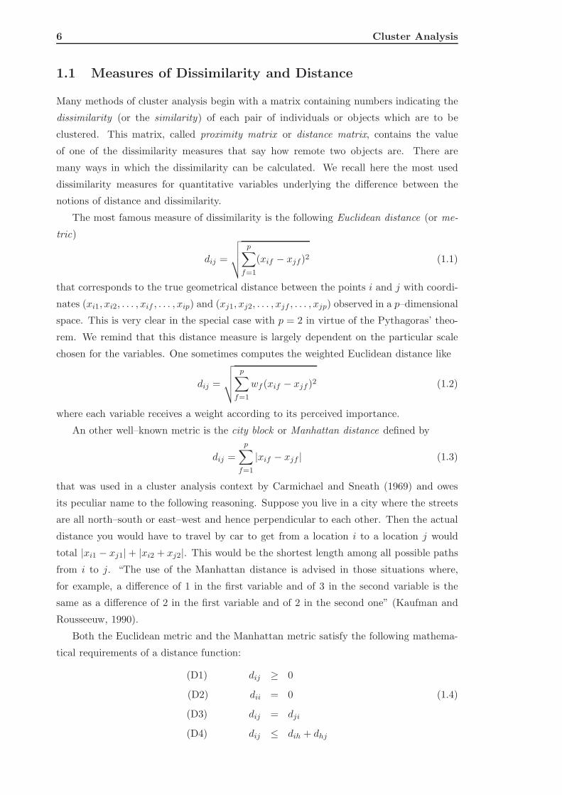
1.1 Measures of Dissimilarity and Distance
Many methods of cluster analysis begin with a matrix containing numbers indicating the
dissimilarity (or the similarity) of each pair of individuals or objects which are to be
clustered. This matrix, called proximity matrix or distance matrix, contains the value
of one of the dissimilarity measures that say how remote two objects are. There are
many ways in which the dissimilarity can be calculated. We recall here the most used
dissimilarity measures for quantitative variables underlying the difference between the
notions of distance and dissimilarity.
The most famous measure of dissimilarity is the following Euclidean distance (or me-
tric)
dij =
√
√
√
√
p∑
f=1
(xif − xjf)2 (1.1)
that corresponds to the true geometrical distance between the points i and j with coordi-
nates (xi1, xi2, . . . , xif , . . . , xip) and (xj1, xj2, . . . , xjf , . . . , xjp) observed in a p–dimensional
space. This is very clear in the special case with p = 2 in virtue of the Pythagoras’ theo-
rem. We remind that this distance measure is largely dependent on the particular scale
chosen for the variables. One sometimes computes the weighted Euclidean distance like
dij =
√
√
√
√
p∑
f=1
wf (xif − xjf )2 (1.2)
where each variable receives a weight according to its perceived importance.
An other well–known metric is the city block or Manhattan distance defined by
dij =
p∑
f=1
|xif − xjf | (1.3)
that was used in a cluster analysis context by Carmichael and Sneath (1969) and owes
its peculiar name to the following reasoning. Suppose you live in a city where the streets
are all north–south or east–west and hence perpendicular to each other. Then the actual
distance you would have to travel by car to get from a location i to a location j would
total |xi1 − xj1|+ |xi2 + xj2|. This would be the shortest length among all possible paths
from i to j. “The use of the Manhattan distance is advised in those situations where,
for example, a difference of 1 in the first variable and of 3 in the second variable is the
same as a difference of 2 in the first variable and of 2 in the second one” (Kaufman and
Rousseeuw, 1990).
Both the Euclidean metric and the Manhattan metric satisfy the following mathema-
tical requirements of a distance function:
(D1) dij ≥ 0
(D2) dii = 0 (1.4)
(D3) dij = dji
(D4) dij ≤ dih + dhj

1.1 Measures of Dissimilarity and Distance 7
for all objects i, j and h. Condition (D1), the distinguishability of non identicals, merely
states that distances are nonnegative numbers and (D2), the indistinguishability of iden-
ticals, says that the distance of an object to itself is zero. Condition (D3) states the
symmetry of the distance function and the (D4) is the triangle inequality. “The latter
says essentially that going directly from i to j is shorter than making a detour over object
h” (Kaufman and Rousseuw, 1990).
We underly that the terms ‘distance’ and ‘metric’ are exchangeable while the terms
‘dissimilarity’ and ‘distance’ are not because, basically, dissimilarities are nonnegative and
symmetric but in general the triangle inequality does not hold. It is often assumed that
dissimilarities satisfy (D1), (D2) and (D3) although there are some clustering methods
that do not require any of them. For completeness, we remind that it is possible to work
with dissimilarity measures dij as well as similarity measures sij and that a similarity
measure bounded to zero and unity is the complement to one of the correspondent dis-
similarity measure. Of course, the similarity degree between two objects increases with
sij and decreases with increasing dij .
A generalization of both the Euclidean and the Manhattan metric is the Minkowsky
distance given by
dij = q
√
√
√
√
p∑
f=1
|xif − xjf |q (1.5)
where q is any real number lager than or equal to 1. This is also called the Lq metric,
with the Euclidean (q = 2) and the Manhattan (q = 1) metrics as special cases.
There are other distances that are not Minkowsky metrics. When it is important
keeping in consideration the correlation between the variables then it is possible to use an
alternative measure called Mahalanobis distance defined by
dij = (xi − xj)′W−1(xi − xj) (1.6)
where (xi) is the p–dimensional vector of observed variables on the unit i and W is the
pooled within–groups variance–covariance matrix. Of course, this matrix will be unknown
a priori and it will be substituted by the overall covariance matrix.
Finally, we remind the Canberra metric, a measure useful only for non–negative varia-
ble defined as follows
dij =
p∑
f=1
|xif − xjf |(xif + xjf )
. (1.7)
Other common measures of dissimilarity are the “1–correlation” distance
dij = 1− ρij = 1−∑p
f=1(xif − xi)(xjf − xj)√
∑pf=1(xif − xi)2
∑pf=1(xjf − xj)2
(1.8)
where xi is the average on unit i and the sum is over the p variables. This measure is
bounded in [0, 2] (objects with correlation 1 and −1, respectively). Variations on this
distance include a version that uses the absolute value of correlation
dij = 1− |ρij|. (1.9)
8 Cluster Analysis
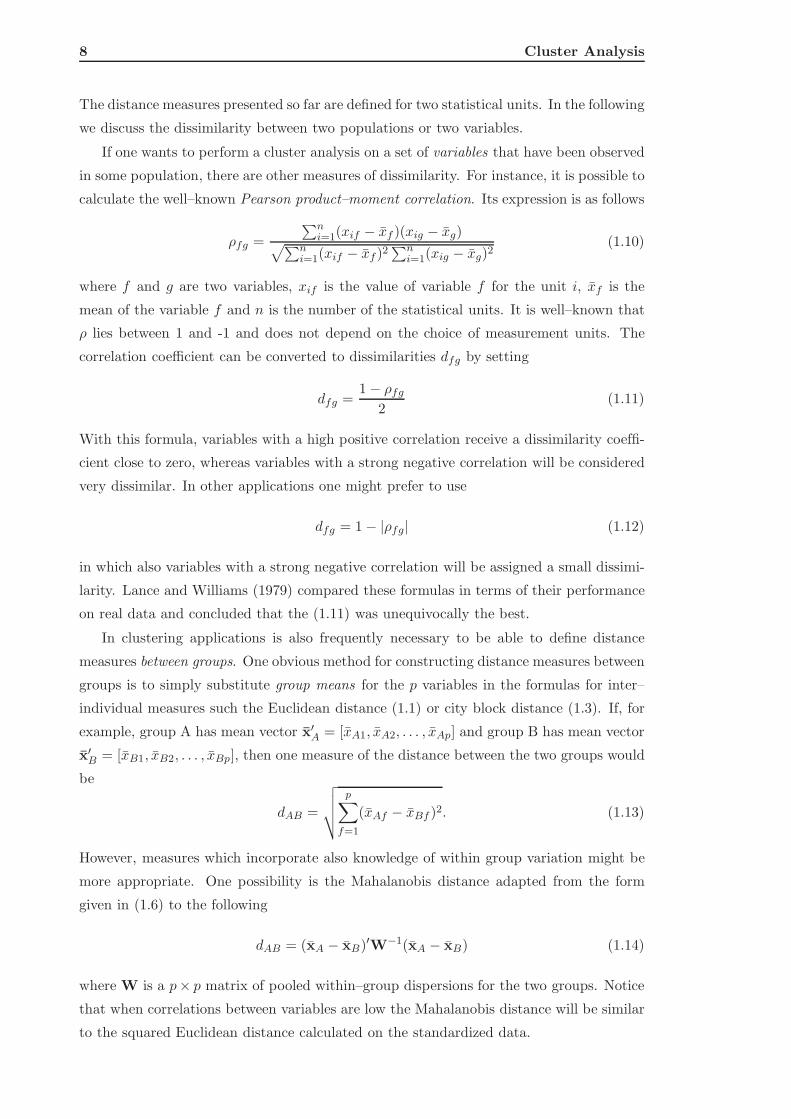
The distance measures presented so far are defined for two statistical units. In the following
we discuss the dissimilarity between two populations or two variables.
If one wants to perform a cluster analysis on a set of variables that have been observed
in some population, there are other measures of dissimilarity. For instance, it is possible to
calculate the well–known Pearson product–moment correlation. Its expression is as follows
ρfg =
∑ni=1(xif − xf )(xig − xg)
√∑n
i=1(xif − xf )2∑n
i=1(xig − xg)2(1.10)
where f and g are two variables, xif is the value of variable f for the unit i, xf is the
mean of the variable f and n is the number of the statistical units. It is well–known that
ρ lies between 1 and -1 and does not depend on the choice of measurement units. The
correlation coefficient can be converted to dissimilarities dfg by setting
dfg =1− ρfg
2(1.11)
With this formula, variables with a high positive correlation receive a dissimilarity coeffi-
cient close to zero, whereas variables with a strong negative correlation will be considered
very dissimilar. In other applications one might prefer to use
dfg = 1− |ρfg| (1.12)
in which also variables with a strong negative correlation will be assigned a small dissimi-
larity. Lance and Williams (1979) compared these formulas in terms of their performance
on real data and concluded that the (1.11) was unequivocally the best.
In clustering applications is also frequently necessary to be able to define distance
measures between groups. One obvious method for constructing distance measures between
groups is to simply substitute group means for the p variables in the formulas for inter–
individual measures such the Euclidean distance (1.1) or city block distance (1.3). If, for
example, group A has mean vector x′A = [xA1, xA2, . . . , xAp] and group B has mean vector
x′B = [xB1, xB2, . . . , xBp], then one measure of the distance between the two groups would
be
dAB =
√
√
√
√
p∑
f=1
(xAf − xBf )2. (1.13)
However, measures which incorporate also knowledge of within group variation might be
more appropriate. One possibility is the Mahalanobis distance adapted from the form
given in (1.6) to the following
dAB = (xA − xB)′W−1(xA − xB) (1.14)
where W is a p× p matrix of pooled within–group dispersions for the two groups. Notice
that when correlations between variables are low the Mahalanobis distance will be similar
to the squared Euclidean distance calculated on the standardized data.

1.2 K–means, Hierarchical and Model–based Clustering 9
A distance measure that geneticists usually use for describing populations in terms of
genes frequencies and called it genetic distance is defined as follows
dAB = (1− cos α)12 (1.15)
where
cosα =∑
i
(piApiB)12 (1.16)
and piA and piB are the gene frequencies for the ith allele at a given locus in the two
populations A and B.
A number of other possibilities for between–group measures which are not based simply
on substituting group in inter–individual measures are available. For example, the distance
between two groups could be defined as the distance between their closest members, one
from each group. This is sometimes known as nearest–neighbour distance and is the basis
of the clustering technique known as single linkage. These measures, called linkage rules,
will be described in the Section 1.2.2, p. 11.
1.2 K–means, Hierarchical and Model–based Clustering
In the introduction to this chapter we have stressed the fact that unsupervised clustering
can be divided in two groups: partitioning and hierarchical methods. Partitioning methods
attempt to find the best solution to group the data for a fixed number K of clusters. In a
hierarchical classification the data are not partitioned into a particular number of classes
or clusters at a single step but the classification consists of a series of partitions which may
run from a single cluster containing all individuals/units to n clusters each containing a
single individual/unit. More precisely, hierarchical clustering techniques can be divided in
agglomerative (bottom–up) and divisive (top–down). The first one proceeds by a series of
successive fusions of the n individuals into groups, that is, they start when all objects are
apart and we have n clusters each one containing only one object; the divisive methods,
instead, separate the n individuals successively into grouping, that is they start from one
cluster containing all the n objects.
In this section we focus our attention on the most popular partitioning method, the
K–means method, on the aggregative hierarchical clustering and on the model–based
clustering.
1.2.1 K–Means Methods
K–means algorithms (MacQueen, 1967; Hartigan, 1975; Hartigan and Wong, 1979) are
among the most popular unsupervised learning algorithms that solve the clustering pro-
blem. In the K–means methods, a cluster is represented through its centroid. The centroid
of a cluster k is defined as a point in p–dimensional space found by averaging the mea-
surement values along each dimension (variable). For example, the centroid of a cluster k

10 Cluster Analysis
is given by
x(k) = (x1(k), . . . , xf (k), . . . , xp(k)) (1.17)
where the generic f–th coordinate is
xf (k) =1
nk
nk∑
ik=1
xikf (1.18)
where ik represents the index of k–th cluster (with k = 1, 2, . . . ,K), which contains nk
objects. Notice that centroids do not have to be one of the objects in the original data
set and they are not defined when the data are dissimilarities not based on interval–scaled
measurement values.
The K–means method finds a partition that minimizes the sum of squared distances
from each observation to its cluster center xf (k), defined as follows
WSS =K
∑
k=1
nk∑
ik=1
||xikf − xf (k)||2. (1.19)
The distance || · || here is the Euclidean distance defined in (1.1) calculated between the
objects of a cluster and its centroid. This method is a part of the so–called variance mini-
mization techniques since it looks for a partition into K subsets that minimizes the within
sum of squares. Many different algorithms have been proposed for variance minimization
techniques and all of them are grouped under the name K–means since all these methods
start by an initial partition of the objects into K non empty subsets. These algorithms
have a common structure of operations that we are going to describe. The algorithm
consists of the following steps:
1. An initial partition of the objects into K non empty subsets is randomly generated.
Then go to step 2. The method can also start with a set of central points (centroids)
in which case one proceeds with step 3.
2. Compute seed points as the centroids of the clusters of the current partition.
3. Assign each object to the cluster with the nearest centroid. The central points
remain fixed for an entire step through the set of objects. If this is the first step, go
to step 2.
4. Update the centroid of each cluster and repeat step 3. In subsequent steps the
clustering is compared to the previous clustering and if no change in the assignment
of objects has occurred, the procedure stops. If there has a change, repeat the step
3. and 4. until any change occur.
The number of clusters is fixed a priori and the procedure consists in calculating one
centroids for each cluster and assigning each observation to one of them. The initial
choice for the centroids has little effect upon the final results even if the better choice is
to place them as much as possible far away from each other. The next step is to take
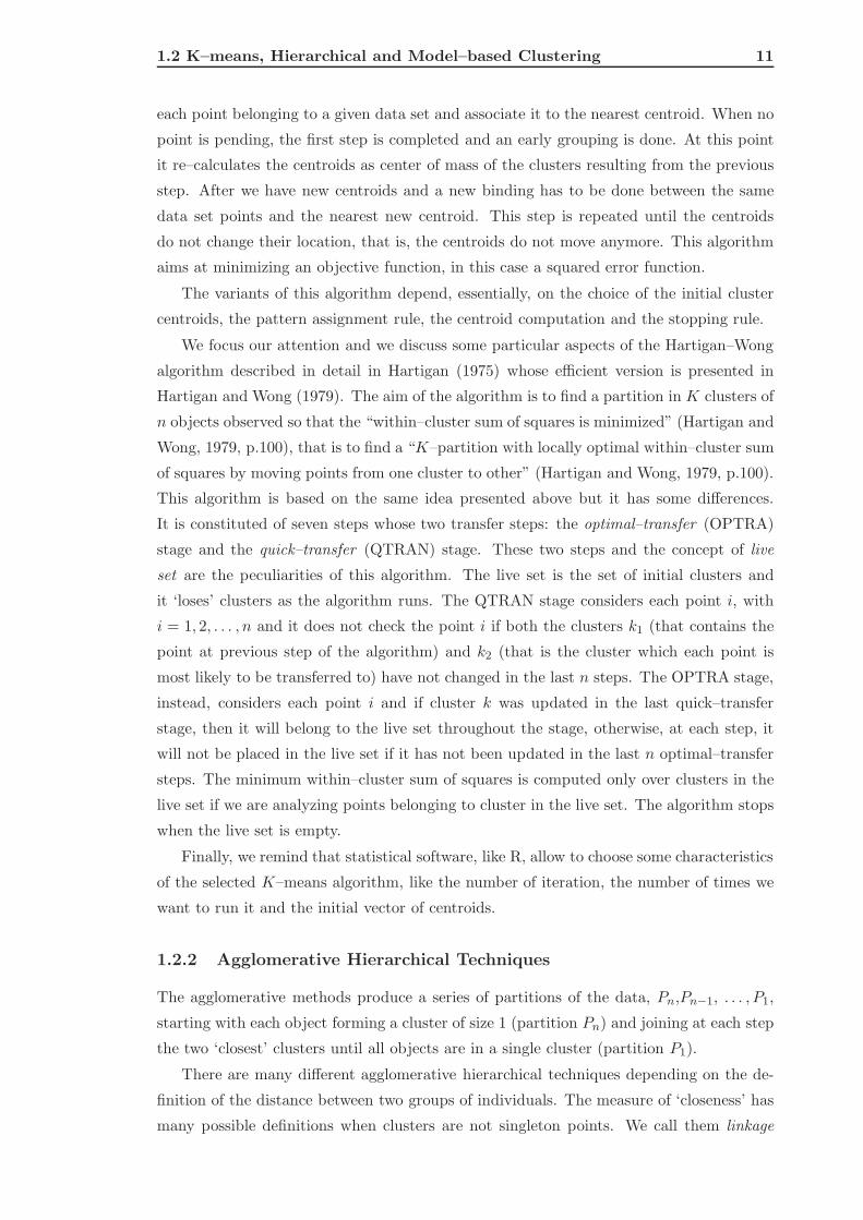
1.2 K–means, Hierarchical and Model–based Clustering 11
each point belonging to a given data set and associate it to the nearest centroid. When no
point is pending, the first step is completed and an early grouping is done. At this point
it re–calculates the centroids as center of mass of the clusters resulting from the previous
step. After we have new centroids and a new binding has to be done between the same
data set points and the nearest new centroid. This step is repeated until the centroids
do not change their location, that is, the centroids do not move anymore. This algorithm
aims at minimizing an objective function, in this case a squared error function.
The variants of this algorithm depend, essentially, on the choice of the initial cluster
centroids, the pattern assignment rule, the centroid computation and the stopping rule.
We focus our attention and we discuss some particular aspects of the Hartigan–Wong
algorithm described in detail in Hartigan (1975) whose efficient version is presented in
Hartigan and Wong (1979). The aim of the algorithm is to find a partition in K clusters of
n objects observed so that the “within–cluster sum of squares is minimized” (Hartigan and
Wong, 1979, p.100), that is to find a “K–partition with locally optimal within–cluster sum
of squares by moving points from one cluster to other” (Hartigan and Wong, 1979, p.100).
This algorithm is based on the same idea presented above but it has some differences.
It is constituted of seven steps whose two transfer steps: the optimal–transfer (OPTRA)
stage and the quick–transfer (QTRAN) stage. These two steps and the concept of live
set are the peculiarities of this algorithm. The live set is the set of initial clusters and
it ‘loses’ clusters as the algorithm runs. The QTRAN stage considers each point i, with
i = 1, 2, . . . , n and it does not check the point i if both the clusters k1 (that contains the
point at previous step of the algorithm) and k2 (that is the cluster which each point is
most likely to be transferred to) have not changed in the last n steps. The OPTRA stage,
instead, considers each point i and if cluster k was updated in the last quick–transfer
stage, then it will belong to the live set throughout the stage, otherwise, at each step, it
will not be placed in the live set if it has not been updated in the last n optimal–transfer
steps. The minimum within–cluster sum of squares is computed only over clusters in the
live set if we are analyzing points belonging to cluster in the live set. The algorithm stops
when the live set is empty.
Finally, we remind that statistical software, like R, allow to choose some characteristics
of the selected K–means algorithm, like the number of iteration, the number of times we
want to run it and the initial vector of centroids.
1.2.2 Agglomerative Hierarchical Techniques
The agglomerative methods produce a series of partitions of the data, Pn,Pn−1, . . . , P1,
starting with each object forming a cluster of size 1 (partition Pn) and joining at each step
the two ‘closest’ clusters until all objects are in a single cluster (partition P1).
There are many different agglomerative hierarchical techniques depending on the de-
finition of the distance between two groups of individuals. The measure of ‘closeness’ has
many possible definitions when clusters are not singleton points. We call them linkage

12 Cluster Analysis
rules.
The simplest technique is single linkage (or the nearest neighbour) that was first de-
scribed by Florek et al. (1951) and later by Sneath (1957) and Johnson (1967). In this
method, the distance between groups is defined as that of the closest pair of individuals,
where only pairs consisting of one individual from each group are considered. Conse-
quently, the dissimilarity between two clusters, dAB , is as follows
dAB = minx∈A,y∈B
||x− y|| (1.20)
where the norm ||x − y|| is a distance or dissimilarity measure defined in Section 1.1 (p.
6) and x is the pattern of unit i in cluster A while y is the pattern of unit j in the cluster
B. This rule produces a chaining effect identifying ‘stretched out’ clusters.
The complete linkage (or furthest neighbour) clustering method is the opposite of the
single linkage in the sense that the distance between groups is now defined as that of the
most distant pairs of individuals from each group. The dissimilarity between two clusters,
dAB , is as follows
dAB = maxx∈A,y∈B
||x− y|| (1.21)
where the norm ||x − y|| is again one of the distance or dissimilarity measure defined in
Section 1.1. This rule performs well when the clusters are compact, roughly spherical and
of equal size.
Both single and complete clustering techniques are invariant under monotone transfor-
mation of proximity, relatively sensitive to outliers and dependent on the metric. Finally,
these two rules represent two extremes in dissimilarity assessment and tend to be sensitive
to atypical patterns since they depend on nearest or furthest neighbors. The next linkage
rule is less sensitive to atypical patterns.
In the group–average clustering, the distance between two clusters is defined as the
average of the distances between all pairs of individuals that are made up of one individual
from each group. The distance between two clusters is given by
dAB =1
nAnB
∑
x∈A
∑
y∈B
||x− y||. (1.22)
This rule does not depend on the number of observations in each cluster and tends to
produce clusters that are a compromise between the shape of clusters produced by single
linkage and those produced by complete linkage.
The centroid based clustering represents groups through their mean value for each
variable, that is, their mean vector x and y, and the inter–group distance is now defined
in terms of distance between them. Of course, the variables must be defined on an interval
scale. The dissimilarity between two clusters is as follows
dAB = ||xA − yB|| (1.23)
A disadvantage of this method is that if the sizes of two groups to be merged are very
different then the centroid of the new group will be very close to that of the larger group

1.2 K–means, Hierarchical and Model–based Clustering 13
and may remain within that group. The centroid method produces a series of merging
distances that might not be increasing due to the fact that the centroids move from one
step to another one.
The Ward ’s method consists in a procedure seeking to form the partitions Pn, Pn−1, . . .
. . . , P1 that minimizes the within sum of squared distances associated with each grouping.
At each step in the analysis, the two clusters that merge are the ones that contribute
to the smallest increase of the overall sum of the squared within–cluster distances. The
dissimilarity between two clusters is as follows
dAB =1
nA + nB
∑
x∈A,B
||x−m||2 (1.24)
where m is the centroid of the merged clusters.
We hint to the work of Eisen et al. (1998) who have proposed a variation of bottom–up
group–average linkage clustering since they define a particular similarity score. We will
describe it in detail in the last section of the Chapter 3.
Remarkably, hierarchical clustering methods have an appealing property in that the
nested sequence of clusters can be graphically represented by a tree called, dendrogram.
Usually, each join in a dendrogram is plotted at a height equal to the dissimilarity between
the two clusters which are joined. Selection of K clusters from a hierarchical clustering
corresponds to cutting the dendrogram with a horizontal line at an appropriate height.
Each branch cut by the horizontal line corresponds to a cluster.
Finally, we remind that statistical software, like R, allow to choose some characteristics
of the hierarchical clustering like the distance measure to produce the proximity matrix
and the kind of linkage rule.
1.2.3 Model–Based Clustering
Model–based clustering (Fraley and Raftery, 1998, 1999, 2000 and 2007) assumes that the
data are generated by a finite mixture of underlying probability distributions
f(x) =K
∑
k=1
τkfk(x) (1.25)
where each probability density function fk(x) is the probability that an observation comes
from the kth mixture component that represents the kth cluster. Usually, multivariate
normal distributions with mean µk and covariance matrix Σk
φk(x|µk,Σk) = (2π)−n2 |Σk|−
12
exp{− 12(xi−µk)′Σ−1
k(xi−µk)} (1.26)
are used for these. For univariate data, the covariance matrix reduces to a scalar variance.
Clusters are ellipsoidal, centered at the means µk while the covariance Σk determine
their other geometric features. The covariance matrix for each cluster can be represented
by its eigenvalues decomposition
Σk = λkDkAkD′k (1.27)

14 Cluster Analysis
where Dk is the orthogonal matrix of eigenvectors, Ak is a diagonal matrix whose elements
are proportional to the eigenvalues, λk is an associated constant of proportionality. They
control, respectively, the orientation, shape, and volume of each cluster. The simplest
forms for the covariance structure can be used, decreasing the number of parameters that
have to be estimated but also decreasing the model flexibility.
The parameters of the model are estimated with an EM algorithm (initialized by
hierarchical clustering) using a fixed value for the number of clusters and a fixed covariance
structure. EM iterates between an ‘E–step’ which computes a matrix whose elements are
an estimate of the conditional probability that an observation belongs to a group k given
the current parameter estimates, and an ‘M–step’ which computes maximum likelihood
parameters given the previously computed matrix. In the limit, the parameters usually
converge to the maximum likelihood values for the Gaussian mixture model
n∏
i=1
K∑
k=1
τkφk(xi|µk,Σk) (1.28)
where φk is the Gaussian density function model and n is the number of observations.
This parameter estimation is then repeated for different numbers of clusters and differ-
ent covariance structures. The result of the first step is thus a collection of different models
fitted to the data and all having a specific number of clusters and a specific covariance
structure. Then, the best model in this group of models is selected. This model selection
step involves the calculation of the Bayesian information criterion (BIC for short) for each
model. In general, the smaller the value of the BIC, the stronger the evidence for the
model and number of clusters. A standard convention for calibrating BIC differences is
that differences of less than 2 correspond to weak evidence, differences between 2 and 6 to
positive evidence, differences between 6 and 10 to strong evidence and difference greater
than 10 to very strong evidence. For the formula of the BIC see Chapter 5, Section 5.1.2,
eq. (5.5), p. 71.
The advantages of the model–based clustering relies mainly on the fact that the availa-
ble statistical inference techniques are well–studied and that there is flexibility in choosing
the component distributions. There are some disadvantages. First, the quality guarantee
of the clusters is a user–defined parameter that is hard to estimate and too arbitrary,
second this algorithm produces clusters all having the same fixed diameter not optimally
adapted to the local data structure, third the computational complexity is high.
For this clustering technique the ‘mclust’ and the ‘mclust02’ R packages are available.
The model options available in these package are two in the case of one dimension: ‘E’ for
equal variance and ’V’ for varying variance while there are ten different models in more
than one dimension each one is given by varying the volumes, the shapes and the orienta-
tion of the clusters producing spherical, diagonal and ellipsoidal distributions (Fraley and
Raftery, 2007).

1.3 Other Clustering Methods 15
1.2.4 Comparison between Clustering Techniques
Clearly the K–means, the agglomerative hierarchical and the model-based clustering me-
thods are totally different. In the following we discuss briefly the differences between these
methods and underly their advantages and disadvantages.
One of the most important disadvantage of the hierarchical clustering is that it opera-
tes on the dissimilarity matrix instead of directly on observations and, consequently, it is
computationally expensive for data with many observations (large n), requiring O(n2) cal-
culations. The K–means algorithm, instead, is fast, as it never evaluates all the n(n−1)/2
pairwise dissimilarities. At each iteration, Kn dissimilarities are evaluated, and the K cen-
troids updated. This speed makes K–means a popular algorithm, allowing it to cluster
thousands of objects. The model–based clustering works directly on the data starting by
a hierarchical (or K–means) classification and has an intermediate computational com-
plexity.
An important practical issue for partitioning methods is how to choose an appropriate
number of clusters. Typically, a partitioning method is run repeatedly for different value of
k, and a loss measure is plotted against the number of clusters. Moreover we have already
discussed the issue of the choice of the initial set of centroids for the K–means method.
Since different solutions will be achieved for different starting values it is good practice
to use multiple runs of the algorithm and choose the partition for which the within sum
of squares is minimized. These two drawbacks are not present in hierarchical methods,
since they produce nested partition of data and it is possible to choose a posteriori the
number of groups even if the level to cut the dendrogram is rather arbitrary. Instead, in
the model–based clustering the EM algorithm runs for different values of the number of
clusters and chooses the K that produces a minimum BIC.
Finally, K–means algorithms do not guarantee a optimal local minimum, as it may be
possible to reassign points to different clusters and further reduce sums of squares. This is
a combinatorial optimization problem, in that in most problems the global optimum will
not be found, and one of possibly many local optima will be instead identified.
1.3 Other Clustering Methods
Sofar we have discussed the K–means, the agglomerative (bottom–up) and the model–
based clustering for the historical and practical importance they have. In this section we
briefly present other clustering techniques proposed in the literature.
The section starts by presenting the top–down hierarchical clustering, then we illu-
strate a method that combines the bottom–up and the top–down clustering. The section
continues with the presentation of two–way clustering methods, block clustering and it
ends with a brief discussion of self organized maps and self organizing tree algorithm.
16 Cluster Analysis
1.3.1 Divisive Hierarchical Methods
We have already mentioned that the idea of the divisive (top–down) hierarchical clustering
consists in finding nested partition of the dataset starting with one cluster containing all
the observations and ending with n clusters, one for each observation. The iterative process
gives rise to a tree structure in which the height of the branches is proportional to the
pairwise distance between the clusters. Like in the agglomerative hierarchical methods,
clusters are formed by cutting the tree at a certain level or height.
To understand why top–down methods are of interest, it is useful to consider weak-
nesses of bottom–up methods. Bottom–up methods can poorly reflect the clusters’ struc-
ture near the top of the tree because many joins have been made at this stage. Each
join depends on all previous joins, so if some questionable joins are made early on, they
cannot be later undone. If we are interested on identifying a few clusters, then top-down
algorithms are likely to produce sensible partitions.
This suggests that hybrid techniques that combine the best of top-down and bottom-
up methods may be useful. There are several variations on top-down clustering, each one
offering a different approach to the combinatorial problem of subdividing a group of objects
into two subgroups. Unlike the bottom-up case, where the best join can be identified at
each step, the best partition cannot usually be found and such methods attempt to find a
local optimum.
1.3.2 Hybrid Hierarchical Clustering
The hybrid hierarchical clustering is a new clustering method defined by Chipman and
Tibshirani (2006) that combines the strengths of bottom–up hierarchical clustering with
that of top–down clustering since the first one is good for identifying small clusters and
the second one is good for identifying a few large clusters. The method is built on the
new hybrid idea of a mutual cluster: a group of points closer to each other than to any
other points. Chipman and Tibshirani established theoretical connections between mutual
clusters and bottom–up clustering methods and illustrate the technique on simulated and
real microarray datasets.
In simulation experiments they compare bottom–up, top–down and hybrid methods
and they found that the hybrid and top–down methods have very low misclassification
rates and a relative within–cluster sum of squared distances (WSS) close to the real value,
with respect to the bottom–up, in the simulation of 50 clusters with 4 observations. When
they work with large clusters of random size they find that misclassification rates and the
WSS are higher than in the other simulations.
Notice that this method is available on R package.

1.3 Other Clustering Methods 17
1.3.3 Two–way clustering
Each clustering method reviewed above works on the row of the data matrix or on its
column finding either clusters of observations or clusters of variables, respectively. A
number of algorithms that perform simultaneous clustering on rows and columns of the
data matrix has been proposed even if they are not yet well–developed and they are not yet
of widespread use. The goal is to find sub–matrices, that is, subgroups of statistical units
and subgroups of variables. These clustering methods are usually called two–way clustering
methods even if they are also referred to in the literature as biclustering, coclustering and
direct clustering, among others names, and have been used in fields such as information
retrieval and data mining as well as in the microarray field.
The most important characteristic of two–way clustering is that it is possible to extract,
simultaneously, joint information about both units and variables. For example, it may be
useful to consider more than one grouping of the variables, based on different subsets of
the units. Getz et al. (2000) propose a two–way clustering method that aims at finding
subsets of the genes that result in stable clusterings of a subset of the samples. That is,
they find pairs of subsets of the genes (rows) and subsets of the samples (columns), so
that when genes are used to cluster samples, the clustering yields stable and significant
partitions. This can be especially useful when the overall clustering of the samples based
on all genes is dominated by some subset of the genes, for example genes related to the
profileration of the cells.
1.3.4 Block Clustering
The block clustering method is a top–down, row–and–column clustering of a data matrix.
It reorders the rows and columns to produce a matrix with homogeneous blocks of the
outcome. Block clustering also produces hierarchical clustering trees for the rows and
columns. The basic algorithm for forward block splitting is due to Hartigan (1972) who
called his approach “direct clustering” but it has become known as block clustering. Here
is an outline of the block clustering procedure:
• begin with the entire data in one block
• at each stage, find the row or column split of all existing blocks into two pieces,
choosing the one that produces the largest reduction in the total within block va-
riance
• use only allowed splits: if there are existing row splits that intersect the block, one
of these must be used for the rows, called a “fixed split”. The same is done for
columns. Otherwise all split points are tried
• the splitting is continued until a large number of blocks are obtained, and then some
block are recombined until the optimal number of blocks is obtained. To find the
18 Cluster Analysis
best split into two groups, one can show that it is sufficient to sort the rows (or
columns) by row (or column) mean, and then seek a split in that order.
A drawback of block clustering when applied to median centered data is that at the start,
all row and columns means are approximately zero. Hence, the procedure has difficulty
getting started. Restricting the choice to fixed splits ensures that: 1) the overall partition
can be displayed as a contiguous representation, with a common reordering for the rows
and columns, 2) the partitions of each of the rows and columns can be described by a
hierarchical tree that has been cut at an appropriate level.
An alternative strategy would be to treat the rows and columns as unordered catego-
rical variables.
1.3.5 SOM and SOTA
The Self organized maps (SOM) (Kohonen, 1990; Herrero et al., 2001) are partitioning
algorithms belonged to the first generation clustering algorithms (Moreau et al., 2002).
These algorithms are constrained so that clusters may be represented in a regular, low–
dimensional structure, such as a grid. This facilitates graphical display: clusters that are
close to one another appear in adjacent cells of the grid. Each of K clusters is represented
by a prototype object. The prototypes are points in the same space as the data, but the
estimation algorithm constrains the prototypes to a low–dimensional, grid–like structure.
The SOM clustering algorithm is quite similar to K–means, but with a constraint
reflecting prototype configuration. For two dimensions, a double indexing scheme of pro-
totypes in the grid space (by row and column) is convenient. Each step of the algorithm
adjusts prototype coordinates using only one of the data points. The grid constraint is
enforced by updates that move not just one prototype toward a data point, but also neigh-
bors (in the grid space) of the nearest prototype. Such an algorithm would typically be
run for several thousand iterations. Initial values of the grid radius would depend on the
number of clusters, but might be chosen so that about a third of all prototypes belong to
the same neighborhood.
Like in SOMs, in the self–organizing tree algorithm (SOTA) the rows data are se-
quentially and iteratively presented to the terminal nodes (located at the base of the
tree). SOTA combines both self–organizing maps and divisive hierarchical clustering. The
topology or node geometry here takes the form of a dynamic binary tree. Subsequently,
the units are associated with the nodes that maps closest to it, and the mapping of this cell
plus its neighboring nodes are updated. After convergence the node containing the most
variable population of units (variation is defined here by the maximal distance between
two units that are associated with the same node) is split into two sister nodes (causing
the binary tree to grow), whereafter the entire process is restarted. The algorithm stops
(the tree stops growing) when a threshold of variability is reached for each cell, which in-
volves the actual construction of a randomized data set and the calculation of the distances
between all possible pairs of randomized rows data.

1.3 Other Clustering Methods 19
One of the advantage of SOTA is that the number of clusters does not have to be
known in advance but the procedure provides for a statistical procedure to stop growing
the tree. Therefore, the user is freed from choosing an (arbitrary) level where the tree has
to be cut (like in standard hierarchical clustering).

Chapter 2
Copula Function
In this chapter we present the copula function from its first definition and its probabili-
stic meaning to its multivariate extension. Then we present different copula estimation
methods.
The second part of this chapter is dedicated to the classes and the families of copula
functions that we present both in the bivariate and in the multivariate case.
2.1 Introduction to the Copula function
Dependence relations between random variables is one of the most widely studied sub-
jects in probability and statistics. The nature of dependence can take a variety of forms
and unless some specific assumptions are made, no meaningful statistical models can be
contemplated.
The copula function allow us to investigate the dependence of a joint distribution
function by means of its marginal distribution functions and one or more dependence
parameters.
After introducing the Frechet bounds, we present copula function as defined in the
Sklar’s theorem (Sklar, 1959). Then we give the probabilistic interpretation of a copula
function and its use in statistics.
2.1.1 Frechet Bounds
Consider a K–variate joint (cumulative) distribution function
F (x1, . . . , xk, . . . , xK) with univariate marginal (cumulative) distribution functions
F1, . . . , Fk, . . . , FK . By definition, each marginal distribution can take any value in the
range [0, 1]. The joint distribution function is bounded below and above by Frechet lower
and upper bounds, FL and FU , defined as
FL(x1, x2, . . . , xk, . . . , xK) = max
[
K∑
k=1
Fk −K + 1, 0
]
(2.1)
FU (x1, x2, . . . , xk, . . . , xK) = min [F1, F2, . . . , Fk, . . . , FK ] . (2.2)
21

22 Copula Function
for all x1, . . . , xk, . . . , xK in RK where R = [−∞,+∞]. Notice that the upper bound is
always a distribution function while the lower bound is a distribution function only in
the bivariate case (K = 2). For K > 2, FL may be a distribution function under some
conditions (see Joe (1997), Theorem 3.6).
2.1.2 Sklar’s Theorem
The concept of ‘copula’ or ‘copula function’ as named by Sklar (1959) originates in the
context of probabilistic metric spaces. The idea behind this concept is the following: for
multivariate distributions, the univariate margins and the dependence structure can be
separated and the latter may be represented by a copula.
The word ‘copula’ is a latin noun that means ‘bond’. The term copula is used in
grammar and logic to describe that part of a proposition which connects the subject
and predicate. In statistics, it now describes the function that ‘joins’ one–dimensional
distribution functions to form multivariate ones and may serve to characterize several
dependence concepts. The copula of a multivariate distribution can be considered as the
part describing its dependence structure as a complement to the behavior of each of its
margins.
Copula functions first appeared in the probability metrics literature through the fol-
lowing Sklar’s theorem (Sklar, 1959):
Theorem 2.1 (Sklar’s theorem) A two–dimensional copula is a function
C : [0, 1]2 → [0, 1] which satisfies the following conditions:
1. C is grounded, that is C(u, 0) = C(0, z) = 0, ∀ (u, z) ∈ [0, 1]2
2. C(u, 1) = u and C(1, z) = z, ∀ (u, z) ∈ [0, 1]2
3. C is two–increasing, that is for every rectangle [u1, u2]× [z1, z2] whose vertices lie in
[0, 1]2, such that u1 ≤ u2, z1 ≤ z2, we have that
C(u2, z2)− C(u2, z1)− C(u1, z2) + C(u1, z1) ≥ 0.
It is straightforward to prove that copulas are bounded:
Theorem 2.2 Copula functions satisfy the following inequality:
W (u, z) = max (u + z − 1, 0) ≤ C(u, z) ≤ min (u, z) = M(u, z) (2.3)
for every point (u, z) ∈ [0, 1]2.
The lower bound is usually denoted by C− and called minimum copula and the upper
bound is denoted by C+ and called maximum copula.
The existence of lower and upper bounds also suggests the following definition of
concordance order. We can say that the copula C1 is smaller than the copula C2, written
C1 ≺ C2, if and only if C1(u, z) ≤ C2(u, z) for every (u, z) ∈ I2. Notice that not all

2.1 Introduction to the Copula function 23
copulas can be compared and that this order is only partial. For detail see Cherubini et
al. (2004).
The multivariate extension of Sklar’s theorem takes the following expression:
Theorem 2.3 (Sklar’s theorem in K dimensions) A copula function is a function C
from the unit cube [0, 1]K to the unit interval [0, 1] that satisfies the following conditions:
1. C is grounded, that is C(u) = C(u1, . . . , uk−1, 0, uk+1, . . . , uK) = 0, for every
u ∈ [0, 1]K
2. its one–dimensional margins are the identity function on [0, 1] : Ck(u) = u,
k = 1, 2, . . . ,K
3. C is K–increasing.
For the definition of K–increasing functions see Cherubini et al. (2004) and Nelsen (2006).
In this context the most important thing is to know that grounded, K–increasing functions
are non–decreasing with respect to all entries (see Cherubini et al., 2004, p. 130).
Analogously to the univariate case, multivariate copulas are bounded:
Theorem 2.4 Every copula satisfies the following inequality:
W = max (u1 + . . . + uK −K + 1, 0) ≤ C(u) ≤ min (u1, . . . , uK) = M (2.4)
∀u ∈ [0, 1]K .
The upper bound is denoted by C+ and satisfies the definition of copula while the lower
bound C− never satisfies it for K > 2. For detail see Cherubini et al. (2004).
2.1.3 Probabilistic Interpretation of Copula Function
We can note that, from the definition of Sklar’s theorem, copulas are joint distribution
functions of standard uniform random variates: C(u1, u2) = Pr(U1 ≤ u1, U2 ≤ u2). We
know that the probability integral transform of random variables X and Y , X → F1(X)
and Y → F2(Y ), are distributed as standard uniform Uk, k = 1, 2: F1(X) ∼ U1 and
F2(Y ) ∼ U2. Also, since copulas are joint distribution functions of standard uniforms, a
copula computed in F1(x), F2(y) gives a joint distribution function in (x, y):
C(F1(x), F2(y)) = Pr(U1 ≤ F1(x), U2 ≤ F2(y))
= Pr(F−11 (U1) ≤ x, F−1
2 (U2) ≤ y)
= Pr(X ≤ x, Y ≤ y)
= F (x, y).
These remarks highlight the link between Sklar’s theorem and its probabilistic meaning.
For the formulation of the following theorem we follow Nelsen (2006).
In terms of distribution functions Sklar’s theorem states the following:

24 Copula Function
Theorem 2.5 (Sklar’s theorem) Let F be a joint distribution function with margins
F1 and F2. Then there exist a copula C such that for all x, y in R
F (x, y) = C(F1(x), F2(y)) (2.5)
If F1 and F2 are continuous, then C is unique. Otherwise, C is uniquely determined on
RanF1 × RanF2, where RanF is the range of the domain of function F . Conversely, if
C is a copula and F1 and F2 are distributions functions, then the function F defined by
(2.5) is a joint distribution function with margins F1 and F2.
Proof: See Nelsen, (2006), p. 21. According to this theorem we can write F (x, y) =
C(F1(x), F2(y)) and split the joint probability into the margins and a copula, so that the
latter only represents the ‘association’ between X and Y .
As a consequence of Sklar’s theorem, the minimum and maximum copulas, C− and
C+, are named respectively the Frechet lower bound and the Frechet upper bound and we
can write as follows
max (F1(x) + F2(y)− 1, 0) ≤ F (x, y) ≤ min (F1(x), F2(y)) (2.6)
that is the Frechet–Hoeffding inequality for distribution functions.
As regards the relationship between the copula function and the dependence measures
the function D(u1, u2) = C(u1, u2) − u1u2 is very interesting since it is equal to zero if
and only if two random variables are independent. Recall that X and Y are independent
random variables if and only if F (x, y) = F1(x)F2(y) and that it is evident that Sklar’s
theorem entails that X and Y are independent if and only if have the product copula
C⊥(u1, u2) = u1u2.
The probabilistic interpretation of a K–dimensional copula function is similar to the
two–dimensional case. For the formulation of Sklar’s theorem we follow Nelsen (2006).
Theorem 2.6 (Sklar’s theorem in K–dimensions) Let F be a K–dimensional joint
distribution function with margins F1, . . . , Fk, . . . , FK . Then there exist a copula C such
that for all x ∈ RK
F (x1, . . . , xk, . . . , xK) = C(F1(x1), . . . , Fk(xk), . . . , FK(xK)). (2.7)
If F1, F2, . . . , Fk, . . . , FK are continuous, then C is unique; otherwise, C is uniquely de-
termined on RanF1×RanF2× . . . RanFk × . . .×RanFK . Conversely, if C is a K–copula
and F1, F2, . . . , Fk, . . . , FK are distribution functions, then the function F defined in (2.7)
is a K–dimensional joint distribution function with margins F1, . . . , Fk, . . . , FK .
Proof: See Nelsen (2006).
As in the two–dimensional case, Sklar’s theorem guarantees that the cumulative joint
probability function can be written as a function of the cumulative marginal ones and vice
versa
F (x) = C(F1(x1), F2(x2), . . . , Fk(xk), . . . , FK(xK)). (2.8)
2.1 Introduction to the Copula function 25
We will say that the random vector X = (X1,X2, . . . ,Xk, . . . ,XK) has the copula C or
that the latter is the copula of X. The generalization of the Frechet–Hoeffding inequality
for multivariate distribution functions is straightforward.
Summarizing, a copula function is a multivariate distribution function with standard
uniform marginal distributions, that is a multivariate distribution function defined on the
K–dimensional unit cube [0, 1]K such that every marginal distribution is uniform on the
interval [0, 1]. In the multidimensional case the possibility of writing the joint cumulative
probability function in terms of the marginal ones allow us to interpret multidimensional
copulas as dependence functions opening the way to a number of different applications.
We will discuss the advantages of using copula functions in statistical modeling in the
next section.
2.1.4 Modeling consequences
According to Sklar’s theorem, any multivariate distribution can be modeled through its
marginal distributions and a copula function separately. Indeed, conceptually, Sklar’s
theorem states that for any bivariate distribution function F (x, y), where F1(x) = F (x,∞)
and F2(y) = F (∞, y) are the univariate marginal probability distribution functions, there
exists a copula C such that F (x, y) = C(F1(x), F2(y)), where we indicate the distribution
C with its cumulative distribution function. The copula contains all the information on the
nature of the dependence between two random variables independently from their marginal
distributions. The information on the marginal distributions and the information on the
dependence are kept separate and their influence can be assessed clearly.
The separation between marginal distributions and dependence parameters explains
the modeling flexibility given by copulas. From theoretical point of view copula functions
allow a double ‘infinity’ of degrees of freedom:
i) define the appropriate margins
ii) choose the appropriate copula
while when modeling from the practical point of view then we can decompose any estima-
tion problem in two steps: the first step is for the margins and the second one is for the
parameters of the copula function. This will be more clear in the next section which will
be dedicated to the estimation methods for copula function.
The advantages of a representation through copula function are many. First of all,
the classical approach to measure dependence, the linear correlation function, is a valid
measure of dependence only within the restrictive class of elliptical distributions. Copula
functions of dependence are free of such limitation. Second, copulas enable to model
the marginal distributions and the dependence structure separately. The former concerns
the shape of the distribution function (such as symmetry, skewness, fat tails and so on),
whereas the copula represents the kind of dependence. Third, one can have combinations
of parametric and non parametric marginal distributions with copulas. Finally, copulas
allow to fit any margin to different random variables and these distributions may vary
26 Copula Function
from one random variables from the next. This has interesting consequences in copula
estimation field.
2.2 Estimation for Copula Functions
In this section we present estimation methods for copula function which have been pro-
posed in the literature.
There is more than one method to estimate copula functions. The most famous method
if the full maximum likelihood (FML, from now on) approach that estimates simultane-
ously all the parameters, that is, those for the margins and those for the copula. A second
method is a sequential 2–step maximum likelihood method, called inference for margins
(IFM, from now on), in which the marginal parameters are estimated in the first step and
are used to estimate the parameter of the copula function in the second step. A third
method is the canonical maximum likelihood (CML, from now on) that is not widely used
in practice consists in estimating the copula parameters without specifying the margins.
We introduce the density of a multivariate copula and then we will present the methods
above cited concentrating our attention on the two–steps method since we will use it on
simulated and real data. In this section we will focus on continuous random variables.
2.2.1 Density of a Copula Function
This section introduces the notions of density and canonical representation of a copula
distribution function.
The density c(u1, . . . , uk, . . . , uK) associated to a copula
C(u1, . . . , uk, . . . , uK) is a function in [0, 1]K as follows:
c(u1, u2, . . . , uk, . . . , uK) =∂KC(u1, u2, . . . , uk, . . . , uK)
∂u1∂u2 . . . ∂uk . . . ∂uK. (2.9)
For continuous random variables, the copula density is related to the density of the distri-
bution F , denoted as f , by the canonical representation
f(x1, . . . , xk, . . . , xK) = c(F1(x1), . . . , Fk(xk), . . . , FK(xK))K∏
k=1
fk(xk) (2.10)
where
c(F1(x1), . . . , Fk(xk), . . . , FK(xK)) =∂KC(F1(x1), . . . , Fk(xk), . . . , FK(xK))
∂F1(x1) . . . ∂Fk(xk) . . . ∂FK(xK)(2.11)
and fk are the densities of the margins
fk(xk) =dFk(xk)
dxk. (2.12)
It is straightforward to find these relationships also in the two–dimensional case in which
the copula density is again equal to the ratio of the joint density f and the product of
the two marginal densities f1 and f2 . From the expression in (2.10) it is clear also that

2.2 Estimation for Copula Functions 27
the copula density takes a value equal to 1 everywhere the original random variables are
independent.
The canonical representation is very useful in statistical estimation, in order to have
a flexible representation for joint densities and in order to determine the copula, if one
knows the joint and marginal distributions.
2.2.2 The FML method
Recalling the canonical representation in (2.10) and in (2.11) we can say that, in general,
a statistical modeling problem for copulas could be decomposed into two steps:
• identification of the marginal distributions;
• definition of the appropriate copula function.
Suppose that we observe n independent realizations from a multivariate distribution in
(2.8),{
(Xi1,Xi2, . . . ,XiK)′ : i = 1, 2, . . . , n}
and suppose that the multivariate distribu-
tion is specified by K margins with cumulative distribution function Fk and probabi-
lity distribution function fk, both with k = 1, 2, . . . ,K, and a copula function c. Let
θ1 = (β′1,β
′2, . . . ,β
′k, . . . ,β
′K)′ be the vector of marginal parameters and θ2 be the vec-
tor of copula parameters. The parameter vector to be estimated is θ = (θ′1,θ
′2)
′. The
log–likelihood function is
l(θ) =n
∑
i=1
log c {F1 (Xi1;β1) , . . . , FK (XiK ;βK) ;θ2}+ (2.13)
+
n∑
i=1
K∑
k=1
log fi (Xik;βk)
The maximum likelihood estimator of θ is as follows
θFML = arg maxθ∈Θ
l(θ) (2.14)
where Θ is, of course, the parametric space.
Throughout this section, we assume that the usual regularity conditions (see Serfling,
1980, and Shao, 1999) for asymptotic maximum likelihood theory hold for the multivariate
model (that is the copula) as well as for all of its margins (the univariate probability density
functions). Under these regularity conditions the maximum likelihood estimator exists and
it is consistent and asymptotically efficient; also, it is asymptotically normal, and we have
√n(θFML − θ0)→ N(0,F−1(θ0)) (2.15)
where F−1(θ0) is the usual Fisher’s information matrix and θ0 is the true value.
The covariance matrix of θFML (Fisher’s information matrix) may be estimated by the
inverse of the negative Hessian matrix of the likelihood function.

28 Copula Function
2.2.3 The IFM method
The maximum likelihood method, previously shown, could be very computationally inten-
sive, especially in the case of a high dimension, because it is necessary to estimate jointly
the parameters of the marginal distributions and the parameters of the dependence struc-
ture represented by the copula. Still, if we look more closely at the log–likelihood function,
we will note that it is composed of two positive terms: one term involving the copula den-
sity and its parameters, and one term involving the margins and all parameters of the
copula density. Starting from this considerations Joe and Xu (1996) proposed a two–stage
estimation method called inference for the margins (IFM). This method is useful because
usually the dimension K (the number of margins) is large. The IFM method estimates
the marginal parameters β in a first step by
θ1IFM = arg maxβ
n∑
i=1
K∑
k=1
log fi(Xik;β) (2.16)
when the marginal distributions have the same parameters β or by an ML estimation for
each margin
βkIFM = arg maxβk
n∑
i=1
log f(Xik;βk) (2.17)
when each marginal distribution Fk has its own parameters βk and θ1 = (β′1, . . . ,β
′k,β
′K)′;
then, in the second step, estimates the dependence parameters θ2 given θ1IFM by
θ2IFM = arg maxθ2
n∑
i=1
log c[
F1
(
Xi1; β1IFM
)
, . . . , FK
(
XiK ; βKIFM
)
;θ2
]
(2.18)
Joe (1997) proved that, like the MLE, the IFM estimator (from the two steps) verifies,
under regular conditions, the property of asymptotic normality, and we have
√n(θIFM − θ0)→ N(0, G−1(θ0)) (2.19)
where G−1 is the Godambe information matrix (Godambe, 1960).
Finally, we stress that the equivalence of the two estimators, ML and IFM, in general,
does not hold. Indeed, calling l the whole log–likelihood function, lk the log–likelihood of
the k–th marginal, and lc the log–likelihood for the copula itself, we have that the IFM
estimator is the solution of the system:
(
∂l1∂β1
,∂l2∂β2
, . . . ,∂lk∂βk
, . . . ,∂lK∂βK
,∂lcθ2
)
= 0′ (2.20)
while the MLE comes from solving
(
∂l
∂β1
,∂l
∂β2
, . . . ,∂l
∂βk
, . . . ,∂l
∂βK
,∂l
θ2
)
= 0′. (2.21)
2.3 Parametric Families of Copula 29
2.2.4 Other estimation methods
In literature other estimation methods, parametric and non–parametric, are available. We
mention the canonical maximum likelihood (CML) estimation, a method for the estimation
of copula parameters without specifying the margins. It could be seen as a maximum
likelihood method given the observed margins. This method could be described as follows
1. estimate the margins via empirical distribution functions without any assumption
on the parametric form of Fk(xik);
2. estimate the copula parameters via the maximum likelihood method maximizing the
following expression
θ2 = arg maxθ2
n∑
i=1
ln c(F1(xi1), . . . , Fk(xik), . . . , FK(xiK));θ2) (2.22)
Notice that it is possible to use also non parametric methods for estimating copula
functions. We just remind the possibility of estimating copula function via kernel copula
using empirical copula and a polynomial approximation for it. For detail see Cherubini et
al. (2004).
2.3 Parametric Families of Copula
In this section we are going to present several families or classes of copulas in their bivariate
representation and, successively, in their multivariate representation. For each family,
we give the definition of the copula function, the parametric space of the dependence
parameters and the properties of the kind of dependence explained by particular models.
2.3.1 Bivariate Copula Functions
Here we present some common bivariate copula functions. We essentially digress on copula
functions for elliptical distributions and about copula functions belonging to the so–called
Archimedean family.
The simplest copula function is the product copula that has the following form
C(u1, u2) = u1u2 (2.23)
where u1 and u2 are uniformly distributed over (0, 1). This copula is important because
it corresponds to the independence case.
The Farlie–Gumbel–Morgenstern (FGM) copula takes the form
C(u1, u2) = u1u2(1 + θ(1− u1)(1− u2)) (2.24)
where the dependence parameter θ is bounded on the interval [−1, 1]; when it is equal
to zero then the FGM copula collapses to independence. This copula was proposed by
Morgenstern (1956) and it is a perturbation of the product copula and it is quite simple but
30 Copula Function
the parametric space of θ does not correspond to either Frechet bound and, consequently,
it is useful when dependence between the two margins is modest in magnitude.
The Normal (Gaussian) copula has the following expression
C(u1, u2) = ΦG
(
Φ−1(u1),Φ−2(u2); θ
)
(2.25)
=
∫ Φ−1(u1)
−∞
∫ Φ−1(u2)
−∞
1
2π(1 − θ2)1/2
{−(s2 − 2θst + t2)
2(1 − θ2)
}
dsdt
where Φ is the cumulative distribution function of the standard normal distribution and
ΦG(u1, u2) is the standard bivariate normal distribution with correlation parameter
−1 < θ < 1. This copula is flexible in that it allows for equal degrees of positive and
negative dependence and includes both Frechet bounds in its permissible range. Notice
that the Gaussian copula function is positively ordered with respect to the parameter, that
is, CGaρ=−1 ≺ CGa
ρ<0 ≺ CGaρ=0 ≺ CGa
ρ>0 ≺ CGaρ=1 and it is comprehensive since CGa
ρ=−1 = C− and
CGaρ=1 = C+.
The Student’s t–copula with θ1 degrees of freedom and correlation θ2 has the following
form
C(u1, u2) =
∫ t−1θ1
(u1)
−∞
∫ t−1θ2
(u2)
−∞
1
2π(1− θ22)
12
{
1 +s2 − 2θ2st + t2
θ1(1− θ22)
}−θ1+2
2
dsdt (2.26)
where t−1θ1
(u1) is the inverse of the cumulative distribution function of the standard uni-
variate t–distribution with θ1 degrees of freedom. This is an example of copula with two
dependence parameters, θ1 and θ2. The first one controls the heaviness of the tails and
the second one is the dependence parameter. When the number of degrees of freedom
diverges, the copula converges to the Gaussian one.
The Clayton copula (1978), also referred to as the Cook–Johnson copula (1981) even
if it was first studied by Kimeldorf and Sampson (1975a, 1975b), takes the following
expression:
C(u1, u2) = (u−θ1 + u−θ
2 − 1)−1θ (2.27)
where the parameter θ is restricted on the region (0,∞). As θ approaches zero, the margins
become independent. As θ approaches to infinity, the copula attains the Frechet upper
bound while this copula can not account for negative dependence.
The Frank copula (1979) is as follows
C(u1, u2) = −1
θln
{
1 +(e−θu1 − 1)(e−θu2 − 1)
e−θ − 1
}
(2.28)
where the dependence parameter θ may assume any real value
(−∞,+∞). Independence is attained as θ reaches zero. Unlike the Clayton copula, the
Frank copula can account for negative dependence and it is symmetric in both tails like the
next two copula functions we present. These two reasons and the fact that the Frenchet
upper and lower bound are included in the range of permissible dependence makes it very
popular and used.
2.3 Parametric Families of Copula 31
The Gumbel copula (1960) takes the form
C(u1, u2) = exp
[
−(
− log uθ1 − log uθ
2
)1θ
]
(2.29)
The dependence parameter takes values in the interval [1,∞). Values of 1 and infinity
correspond to independence and the Frechet upper bound, respectively, but, as the Clayton
copula it does not allow negative dependence.
The last three copula functions belong to the Archimedean Copulas. The Archimedean
family of copula functions has been proven useful in empirical modeling and it is popular
because of ease of derivation. Bivariate Archimedean copulas take the general following
form
C(u1, u2) = γ−1 (γ(u1) + γ(u2)) (2.30)
where γ−1 is the inverse of the (strict) generator γ(u) : [0, 1]→ [0,∞] and the dependence
parameter θ is imbedded in the functional form of the generator γ. In order for (2.30)
to be a copula, the generator needs to be a complete monotone function. A generator
uniquely defines an Archimedean copula. For the details see Nelsen (2006). Finally,
Archimedean copulas are symmetric, that is, C(u1, u2) = C(u2, u1), and associative, that
is C(C(u1, u2), u3) = C(u1, C(u2, u3)).
Notice that there one a lot of different copula functions belonging to the Archimedean
family and a lot of different families or classes of copula functions but they are not very
used in practical applications also for their analytical complexity. For an extended review
see Nelsen (2006) and Joe (1997).
2.3.2 Multivariate Copula Functions
In this section we present the copula functions presented till now giving their multivariate
definitions and the parametric space of their parameter/s.
The multivariate Farlie–Gumbel–Morgenstern (FGM) copula (Johnson and Kotz, 1975)
has the following extension to a (2K −K − 1)–parameter family of K–copulas, K ≥ 3:
C(u1, . . . , uk, . . . , uK) = u1 . . . uk . . . uK
[
1 +
K∑
k=2
(2.31)
∑
1≤j1≤...≤jk≤K
θj1j2...jk(1− uj1) . . . (1− ujk
)
where each parameter must satisfy |θ| ≤ 1. Note that each k–margin, 2 ≤ k ≤ K, of an
FGM K–copula is an FGM k–copula. For detail see Nelsen (2006).
The multivariate Normal (or Gaussian) copula has the following expression:
C(u1, . . . , uk, . . . , uK) = ΦG
[
Φ−1(u1), . . . ,Φ−k(uk), . . . ,Φ
−K(uK); θ]
(2.32)
where Φ is the cumulative distribution function of the standard univariate normal distri-
bution.

32 Copula Function
The multivariate Students t–copula (MTC) is as follows
C(u1, . . . , uk, . . . , uK) =∫ t−1
ν (u1)−∞ . . .
∫ t−1ν (uk)
−∞ . . .∫ t−1
ν (uK)−∞
Γ( ν+n2 )|R|−
12
Γ( ν2 )(νπ)
n2
(2.33)(
1 + 1ν x
′R−1x)− ν+K
2 dx1 . . . dxk . . . dxK
where t−1ν is the inverse of the univariate cumulative distribution function of Student’s t
with ν degree of freedom and R is the correlation matrix.
The Clayton K–copula has the following expression:
C(u1, . . . , uk, . . . , uK) =
[
K∑
k=1
u−θk −K + 1
]− 1θ
(2.34)
where the parameter θ restricted on the region (0,∞). As θ approaches zero, the marginal
distributions become independent.
The multivariate Frank copula is as follows:
C(u1, . . . , uk, . . . , uK) = −1
θln
{
1 +
∏Kk=1(e
−θuk − 1)
(e−θ − 1)K−1
}
(2.35)
with θ ∈ (0,∞) as long as K ≥ 3. θ = 0 corresponds to independence.
The multivariate Gumbel copula is as follows
C(u1, . . . , uk, . . . , uK) = exp
−[
K∑
k=1
(− ln uk)θ
]
1θ
(2.36)
with θ > 1.
Finally, we generalize the generator of the Archimedean copula functions recalling the
expression in (2.30). A multivariate Archimedean copula is constructed through a (strict)
generator γ as
C(u1, . . . , uk, . . . , uK) = γ−1 (γ(u1), . . . , γ(uk), . . . , γ(uK)) (2.37)
where γ−1 is the inverse of the (strict) generator γ and in order for (2.37) to be a copula,
the generator needs to be a complete monotone function.
For an extended review of classes of copula functions see Nelsen (2006) and Joe (1997).
Chapter 3
Microarray Experiments
This chapter is dedicated to the biological and genetic concepts relevant to understand
the birth of the theoretical ideas at the basis of our work and the kind of applications
involved. After a brief introduction to DNA, genes and the genetic code, we explain what
a DNA microarray and microarray technology are, how it is possible to produce microarray
data and which kinds of microarray experiments exist in the literature. We conclude this
chapter by a section on the applications of cluster analysis and copula functions introduced
in the previous chapters to the microarray and genetic data.
3.1 DNA, RNA, Gene Expressions and Microarray
In this section we introduce the background of microarray experiments. We introduce
the concepts of DNA, gene and genetic code, as well as the basic of gene expression and
microarray analysis.
3.1.1 DNA and the Central Dogma
The deoxyribonucleic acid (DNA) is the most important macromolecule that controls
most of the activities of life. The genetic material of all known organisms consists of
one or more long molecules of DNA. It is made up of chains of chemical building blocks
called nucleotides and each nucleotide consists of a phosphate group, a deoxyribose sugar
molecule, and one of four different nitrogenous bases usually referred to by their initial
letter: Guanine (G), Adenine (A), Cytosine (C) and Thymine (T). Genetic information
is encoded in DNA through sequences of these nucleotides that are connected each other
via a link of the 5’ 1 hydroxyl phosphate group of one pentose ring of the deoxyribose
sugar to the 3’ OH group of the next pentose ring. It is conventional to write nucleic acid
sequences in the direction from the 5’ end to the 3’ end and each chain is said to have
polarity. DNA forms a double helix of two intertwined chains called strands of nucleotides.
The two chains run in opposite directions. It was proposed in the famous work of Watson
1The carbons in the deoxyribose sugar group of a nucleotide are assigned numbers followed by a prime
symbol (1’,2’. . . ).
33

34 Microarray Experiments
DNA-
Replication DNA
RNA
Reverse
TranscriptionTranscription
RNA-
Replication
Translation
Protein
The Central Dogma of Molecular Biology
Figure 3.1: Central Dogma of Molecular Biology
and Crick (1953) that the two nucleotide chains are held together by hydrogen bounds
between the nitrogenous bases. The polarity of the double helix requires specific hydrogen
bonding between the bases so that they fit together. Guanine pairs only with cytosine
whereas adenine only with thymine and these bases are said complementary.
Each cell contains a complete copy of its genetic material in the form of DNA molecules.
The genetic information can be copied as a transportable copy composed of ribonucleic
acid (RNA) molecules. This process is called transcription. The RNA is transferred to
a machinery that synthesizes protein molecules based on the information carried by the
RNA. This process is called translation. The process sequence from DNA to RNA and
from RNA to protein is called the central dogma of molecular biology (see Fig. 3.1) that
formulates how the information is stored and converted to all components and interactions
that build up a living organism.
3.1.2 Genes, RNA, Genetic Code and Proteins
Genes are the units of the DNA sequence that control the hereditary traits of an organism.
A gene can be defined as a segment of DNA that defines a functional RNA.
There are two general classes of RNA: messenger RNA (mRNA) and functional RNA,
that is the transfer RNA (tRNA) and the ribosomal RNA (rRNA). The mRNA takes part
in the process of decoding of genes in sequences of amino acids while the functional RNAs
take part into the protein synthesis machinery that translates the mRNA into proteins.
The sequences of nucleotides are important because they code for sequences of amino acids
that dictate the structure of a protein with a defined function. The relationship between a
sequence of DNA and the sequence of the corresponding protein is called the genetic code.

3.2 DNA Microarray 35
The genetic code is read in groups of three nucleotides, or codons, each of which
represents one amino acid. There are 43 = 64 different codons because each position can
be occupied by one of the four nucleotides. As there are only 20 amino acids, several
different codons can code for the same amino acid. Consequently, the genetic code is said
to be degenerate for this many–to–one relationship. A line chain of building blocks called
amino acids is the primary structure of a protein.
The total set of genes carried out by an individual or a cell is called its genome that
defines the genotype. Today the complete genome sequences of several species are known.
With microarray experiment we can study all the genes of an organism simultaneously.
3.1.3 Gene Expression, Microarray and cDNA
Gene expression is the process by which the mRNA, and eventually a protein, is synthe-
sized from the DNA template of each gene. The first stage of this process is transcription,
where a DNA copy of one strand of the DNA is produced. In the eukaryotes organisms this
is followed by RNA splicing during which the introns are cut out of the primary transcript
and a mature mRNA is made. Transcription and splicing occur in the nucleus. The next
stage is the translation of the mRNA into protein. This occur in the cytoplasm. In the
process of the gene expression, RNA provides not only the essential substrate (mRNA)
but also components of the protein synthesis apparatus (tRNA and rRNA).
A microarray is typically a glass or a polymer slide onto which DNA molecules are
attached at fixed locations called spots or features. There are may be tens of thousands of
spots on an array, each containing tens of millions of identical DNA molecules of lengths
from tens to hundreds of nucleotides. For gene expression studies, each of these molecules
should identify a single mRNA molecule, or transcript, in a genome.
Complementary DNA (cDNA) is used in recombinant technology and it is complemen-
tary to a given mRNA and it is usually made by the enzyme reverse transcriptase that
allows a mature mRNA to be retrieved as cDNA without the interruption of non–coding
introns (see Fig. 3.1). In microarray technology the process of reverse transcription is
frequently used to incorporate fluorescent dyes into cDNA to the mRNA transcripts.
3.2 DNA Microarray
A DNA microarray, called also gene chip or DNA chip or gene array, is a collection
of microscopic DNA spots attached to a solid surface, such as glass, plastic or silicon
chip forming an array for the purpose of expression profiling, monitoring expression levels
for thousand of genes simultaneously. The affixed DNA segments are known as probes
(although some sources will use different nomenclature such as reporters), thousands of
which can be placed in known locations on a single DNA microarray.
Microarray technology is still developing rapidly, so that there are not established stan-
dards for microarray experiments, for processing of the raw data and for measuring gene

36 Microarray Experiments
expression levels. The Microarray Gene Expression Data Society (MGED) has developed
recommendations for ‘Minimum Information About a Microarray Experiment (MAIME)’,
that attempt to define the set of information sufficient to interpret the experiment and
the results of the experiment. It is possible to find these criteria in Brazma et al. (2000).
Measuring gene expression using microarray is relevant to many areas of biology and
medicine, such as studying treatments and disease. Microarray may be used to measure
gene expression levels in different ways.
3.2.1 Microarray Technology
Microarray allow large numbers of DNA clones with known sequences to be immobilized
as an array of detection units (probes) while the pool of RNAs to be examined (targets) is
fluorescently labeled and then hybridized to the detectors. There are three main microar-
ray technological platforms, namely spotted cDNA arrays, spotted oligonucleotide arrays
and in–situ oligonucleotide arrays. The differences between these three platforms lie in
the way the arrays are produced and the types of probes used.
In spotted microarray or two–channel or two–colour microarrays, the probes are cDNA
or oligonucleotides. When this kind of array is hybridized with cDNA from two sam-
ples to be compared (for example, patient and control) that are labeled in two different
fluorophores (for example, green and red usually labeled by Cy3 and Cy5, respectively),
the samples can be mixed and hybridized to one single microarray that is successively
scanned, allowing the visualization of up–regulated and down–regulated genes in one go.
The downside of this procedure is that the absolute levels of gene expression cannot be
observed, but only one chip is needed per experiment.
In oligonucleotide microarray or single–channel microarrays, the probes are designed
to match parts of the sequence of known or predicted mRNAs. There are commercially
available designs that cover complete genomes from some companies and these microar-
rays give the estimations of the absolute value of the gene expression and therefore the
comparison of two conditions requires the use of two separated microarrays.
In–situ oligonucleotide arrays use a combination of photolithography and solid–phase
oligonucleotide chemistry to synthesize short nucleotide probes directly on the solid sup-
port surface. The test and the reference samples are hybridized separately on different
chips while for either spotted cDNA arrays or spotted oligonucleotide arrays, a test and a
reference sample labeled with two different fluorescent dyes are simultaneously hybridized
on the same array.
3.2.2 Data generation
It is possible to divide each microarray experiment in two main parts, each one consisting
of different steps. The first part is the material processing and data collection and the
second one is the information processing. We follow the scheme in Causton, Quackenbush
and Brazma (2003).
3.2 DNA Microarray 37
The material processing and data collection can be divided in the following steps:
1. array fabrication
2. preparation of the biological samples to be studied
3. extraction and labeling of RNA from the samples
4. hybridization of the labeled extracts to the array
5. scanning of the hybridized array.
The starting point for information processing is the scanned image.
The information processing can be also divided into distinct stages:
6. image quantification, that is localization of the spots on the image and measurement
of their fluorescence intensities
7. data normalization and integration, that is constructing the gene expression data
matrix that describes values from sets of spot quantifications from different hy-
bridizations
8. gene expression data analysis, e.g. finding differentially expressed genes or clusters
of similarity expressed genes
9. generation of new hypotheses about the underlying biological processes
Hybridization of the labeled target to the probes on a microarray is performed by adding
the targets dissolved in hybridization buffer to the slide within a confined space, followed
by incubation for a given amount of time at a certain temperature. The hybridization can,
for example, be performed under a microscope slide cover slip. Automated hybridization
stations that agitate the hybridization solution over the slide and allow for better control
of hybridization conditions have been developed and this gives lower backgrounds and
better reproducibility.
After hybridization, an image of the array with hybridized fluorescent dyes must be
acquired. Microarray scanners have confocal lasers or other light sources to produce light at
the wavelength that excites the fluorescent dyes. The fluorescent emission intensity of the
dyes is captured in high–resolution monochrome images acquired for each fluorescent dye.
The scanner software then displays a composite colored image for multi–dye hybridizations.
The goal is to measure, for each spot on the array, the relative amount of fluorescence
from each dye hybridized with its target. Next, the probe spots have to be identified and
the fluorescence intensities quantified from the high–resolution image.
An essential feature of all the imagine analysis softwares is that the digitized microarray
images are processed and the data are extracted and combined in a table. This is known as
a spot quantitation matrix. Each row corresponds to one spot on the array and each column
represents different quantitative characteristics of that spot, such as mean or median pixel

38 Microarray Experiments
intensity of the spot and local background. Generation of the spot quantitation matrix is
only an intermediate stage in data processing. The data from multiple hybridizations must
be further transformed and organized in a gene expression matrix. In this matrix each row
represents a gene (or transcript) by the index g = 1, 2, . . . , G and each column represents
a sample or an experimental condition by the index s = 1, 2, . . . , S, such as a particular
biological sample. Each position in such a matrix characterizes the expression level of a
particular gene under a particular experimental condition. Here a general expression:
x11 . . . x1s . . . x1S
... . . .... . . .
...
xg1 . . . xgs . . . xgS
... . . .... . . .
...
xG1 . . . xGs . . . xGS
(3.1)
The simultaneous hybridization of two specimen samples labeled with Cy3 (green) and
Cy5 (red) dyes has special analysis requirements. The fluorescence signals from the two
dye channels have to be normalized in order to calculate correct expression ratios. Nor-
malization not only corrects for different dye properties but also for concentration diffe-
rences between the co–hybridized test and reference samples. In practice, expression data
obtained from either spotted cDNA arrays or spotted oligonucleotide arrays are often re-
ported as an expression ratio. The expression ratio is simply the normalized ratio of the
fluorescence intensity of the test sample and the reference sample for a given gene.
The material processing steps are preceded by information processing in the experi-
mental design to which we dedicate the next section.
3.3 Experimental Designs
Microarray data provide information about the overall amount of mRNA in a sample,
therefore differences in mRNA abundance detected using microarrays reflect not only
differences in gene expression but also any differences in the composition of the sample.
The amount of mRNA can be considered a reflection of the expression level of a transcript
only if the samples are relatively homogeneous and the stability of the transcript does not
change between the conditions being compared. The used experimental design play an
important role in the analysis of the gene expression data.
In this section we briefly present a selective review of experimental design issues arising
in a microarray experiment.
3.3.1 The Main Experimental Designs
It is possible to divide the types of experimental designs by the number of factors involved
in the experiments and by the structure of the experiment. The different setting that a
factor may take on in an experiment are referred to as factor levels.

3.3 Experimental Designs 39
A microarray experiment that involves only one factor may be suited for assessing
changes in gene expressions across a single factor of interest. A one–way comparison of
the expression levels across factor levels can be used to identify a differentially expressed
gene.
In a two–way analysis, there are two factors involved in the comparison. For example,
if we have two types of mice, mutant and wild type, and we are interested in observing the
toxin exposure, which has three levels, according to the kind of mouse, then the two–way
factor structure consists of six combinations of levels.
When there are more than two factors involved in the experiment, the multi–way
structure is often called a factorial design. An S–way factorial design consists of S factors
having k1, k2, . . . , kS levels, respectively. If all possible k1 × k2 × . . . × kS combinations
levels are taken into account, then the design is called complete factorial design.
When the number of factors in an experiment is large, the number of possible combina-
tions of the factor levels required for a complete factorial design is huge and it is necessary
to use only a subset of all possible combinations of factor levels. This chosen subset is
called a fractional replication or a fractional factorial design.
After having decided the number of factors and their levels involved in the experiment,
it is necessary to decide the structure of the experimental design. We have the completely
randomized design that is an experiment in which a random sample of statistical units
drawn from the population are randomly assigned to the factor levels. If an equal number
of mice are assigned to each treatment, then the design is called balanced.
The randomized complete block design was born in agricultural experiment and, in
genetic experiments, it can reduce variability improving the detection of significant diffe-
rences. For example, multiple RNA samples taken from the same mouse could be used for
different treatments so as to eliminate possible intra–sample variations. The S treatments
of interest would be randomly assigned to S RNA samples from each of the mice. When
the number of treatment conditions matches the number of experimental units in each
block, as in this example, the design is called a randomized complete block design.
The incomplete block design is a design with the number of experimental units in each
block less than all possible treatment conditions of interest. For example, if only two RNA
samples are available for each of 4 mice and there are four treatment conditions of interest,
then only two of fours treatments can be applied to each mouse.
The balanced incomplete block design (BIBD) is an incomplete block design where all
treatments are replicated the same number of times and any pair of treatments appears
together equally often within blocks.
Finally, when each level of one factor can not be observed in combination with each
level of any other factor in a multi–factor study, the factors cannot be crossed. In these
experiments the factors may be nested and the designs are called nested designs. Nesting
refers to the condition where all levels of one factor are found within only one level of
a second factor. In the design structure of an experiment, nested effects occur when the

40 Microarray Experiments
experimental units for one factor are different for each experimental unit of a second factor.
In the next section we focus on some widely used experimental designs in the context
of microarray analysis that will be of interest for our applications.
3.3.2 Experimental Designs in Microarray Studies
In microarray experiment it is very common to use the reference design in which the
variation in the RNA from spot to spot can be controlled by having the same reference
RNA sample on each spot. A common practice is to compute ratios of the raw signals
as estimates of differential expression between the two samples spotted together. For
example, Alizadeh et al. (2000), to study molecular classification of human lymphomas
designed the Lymphochip by selecting genes that are preferentially expressed in lymphoid
cells and genes with suspected roles in processes important in cancer or immunology. A
fluorescent cDNA sample, labeled with Cy5 dye, was prepared from each experimental
mRNA sample. A reference cDNA sample, labeled with Cy3 dye, was prepared from
a pool of mRNAs isolated from nine different lymphoma cell lines. Each Cy5–labeled
experimental cDNA sample was combined with the Cy3-labeled reference sample and
the mixture was hybridized to the microarray. The fluorescent ratio was determined for
each gene and gene expression measurements were obtained for normal and malignant
lymphocyte samples using Lymphochip microarrays.
The time–course experiment is often used in microarray studies because knowing when
and where a gene is expressed can provide a strong clue about its biological role. A common
set up for this kind of experiment is similar to the design previously described. DeRisi et al.
(1997) conducted a systematic investigation of gene expression of the yeast Saccharomyces
cerevisiae. In their experiment, cells from yeast culture were inoculated into fresh medium
and grown for 21 hours. After an initial 9 hours of growth, samples were harvested at seven
successive 2–hour intervals. They labeled the cDNA prepared from cells at each successive
time point with Cy5, then mixed it with at Cy3–labeled ‘reference’ cDNA sample prepared
from cells harvested at the first interval after inoculation. We note that a short time course
experiment can be regarded as a single factor experiment with time as a factor. What
makes it different from other single factor experiments is the additional information from
the natural ordering of time course samples.
The reversed–color design allow us to eliminate the confounding between treatments
effects and dye effects typical of a reference design in which one dye is used to label
the reference sample and another dye is used to label other treatment samples. This
confounding can be eliminated by repeating the experiment with the dye colors reversed.
In the loop design, the S pairs of treatments (t1, t2), (t2, t3), . . . , (tS−1, tS), (tS , t1) are
spotted on two arrays with color channel reversed for one array relative to its mate.

3.4 Data Analysis for Gene Expression Data 41
3.4 Data Analysis for Gene Expression Data
The first published microarray used for gene expression profiling was in the 1995 by Schena
et al. (1995) and the first complete eukaryotic genome, the Saccharomyces cerevisae, on
a microarray, that is the first use of microarray to study global gene expression, was
published in 1997 by DeRisi et al., both on Science.
Microarray data analysis is based on the hypothesis that there are biologically relevant
patterns to be discovered in the data. For example, there may be genes whose patterns of
expression either allow the samples to be classified or reflect specific cellular responses.
The analysis of a DNA microarrays poses a large number of statistical problems and
many statistical methods have been used on microarray data. In the literature it is possible
to find a very large set of statistical applications, from ANOVA models to Principal Com-
ponents, from Artificial Neural Networks to Support Vector Machines, from Hierarchical
Bayes Methods to Mixture Models, from Discriminant Analysis to Survival Analysis. A
basic difference between the traditional biomedical research and the microarray data ana-
lysis is the dimensionality of the data. A microarray study is typically performed on one
hundred samples, each of which consisting of many thousand of observations. One of the
first used statistical tool is the technique for reducing the dimensionality of the data so
that it is possible to visualize them.
In this section we discuss briefly the preprocessing phase of the data and we present
some applications of clustering methods and copula functions to microarray data.
3.4.1 Preprocessing of the Data
Before clustering or other methods can be applied to microarray data it is necessary to
perform some additional operations on the data. The most common preprocessing steps
are:
1) Normalization of the hybridization intensities within a single array experiment. In
a two–channel cDNA microarray experiment, several sources of noise (such as diffe-
rences in labeling, in detection efficiency, and in the quantity of initial RNA within
the two channels) create systematic sources of biases. These biases can be assessed
and removed. Since many sources of distortion can be considered and since they
can be estimated and adjusted in a variety of ways, many different normalization
procedures exist;
2) Nonlinear Transformations: it is common practice to pass expression values through
a nonlinear function, often the logarithm transformation is used. This is especially
suited for dealing with expression ratios (coming from two–channel cDNA microarray
experiments, using a test and reference sample), since expression ratios are not
symmetrical. Up–regulated genes have expression ratios between one and infinity,
while down–regulated genes have expression ratios squashed between one and zero.

42 Microarray Experiments
Taking the logarithms of these expression ratios will produce a symmetry between
expression values of up– and down–regulated genes. For detail see Moreau et al.
(2002).
3) Missing Values (due to technical reasons) Replacement: the inability of many cluster
algorithms to handle such missing values, like the K–means methods, needs the
imputation of these values. Simple replacements such as a replacement by zero
or by the average of the expression profile often disrupt these profiles. Indeed,
replacement by average values relies on the unrealistic assumption that all expression
values are similar across different experimental conditions. Because of an erroneous
missing value replacement, genes containing a high number of missing values can be
assigned to the wrong cluster. More advanced techniques of missing value imputation
(which use the nearest neighbor method or the singular value decomposition) take
advantage of the rich information provided by the expression patterns of other genes
in the data set. Finally, note that some implementations of algorithms use only the
measured values to derive the clusters and as such obviate the need for missing value
replacement.
4) Filtering: a set of microarray experiments, generating gene expression profiles, fre-
quently contain a considerable number of genes that do not really contribute to
the biological process that is being studied. The expression values of these pro-
files often show little variation over the different experiments even if they will have
seemingly random and meaningless profiles after standardization. Filtering removes
gene expression profiles from the data set that do not satisfy some simple criteria.
Commonly used criteria include a minimum threshold for the standard deviation of
the expression values in a profile and a threshold on the maximum percentage of
missing values.
5) Standardization or Rescaling: Biologists are mainly interested in grouping gene ex-
pression profiles that have the same relative behavior. Genes showing the same
relative behavior but with diverging absolute behavior will have a relatively high
Euclidean distance. Cluster algorithms based on this distance measure will there-
fore wrongfully assign these genes to different clusters. This effect can largely be
prevented by applying standardization or rescaling to the gene expression profiles to
have zero mean and unit standard deviation. Gene expression profiles showing the
same relative behavior will have a small(er) Euclidean distance after rescaling.
3.4.2 Clustering for Gene Expression Data
Clustering is one of the most used unsupervised method in gene expression data analysis.
For microarray data, clustering may be applied to the genes whose expression levels are
measured with the expectation that functionally related co–regulated genes will show
expression patterns. On the other hand, one may use clustering to analyze the expression

3.4 Data Analysis for Gene Expression Data 43
profiles of a set of cell or tissue samples with the hope that samples with similar biological
characteristics will be grouped together.
Cluster algorithms are explicitly or implicity based on a quantitative measure of dis-
similarity between the objects of interest. In the case of row and column vectors of a gene
expression data matrix, typical examples are the Euclidean distance in (1.1) (p. 6) or 1
minus the correlation coefficient (eq. (1.9) p. 7 and/or eq. (1.12), p. 8).
The first application of a cluster analysis on microarray data was made by Eisen et
al. (1998). They worked on the gene expression in the budding yeast Saccharomyces
cerevisiae by means of the hierarchical clustering based on a measure of distance that is
a form of the correlation coefficient. For any two genes X and Y observed on a series of
S conditions, this measure is as follows
dE(X,Y ) =1
S
S∑
s=1
(
Xs −Xoffset
σx
)(
Ys − Yoffset
σy
)
(3.2)
where
σX =
√
√
√
√
S∑
s=1
(Xs −Xoffset)2
S(3.3)
and similarly for Y . When Xoffset is set to the mean of observations on X, then σX becomes
the standard deviation of X and dE(X,Y ) is exactly equal to the Pearson correlation
coefficient of the observations of X and Y .
Values of Xoffset which are not the average over observations on X are used when there
is an assumed unchanged or reference state represented by the value of Xoffset, against
which changes are to be analyzed. In all of the examples presented in Eisen et al. (1998),
Xoffset is set to 0, corresponding to a fluorescence ratio of 1.0. They use a hierarchical
clustering algorithm to compute a dendrogram that assembles all elements into a single
tree. For any set of g genes by using eq. (3.2) an upper–diagonal similarity matrix which
contains similarity scores for all pairs of genes is computed. The matrix is scanned to
identify the highest value representing the most similar pair of genes. A node is created
joining these two genes, and a gene expression profile is computed for the node by averaging
observation for the joined elements (missing values are omitted and the two joined elements
are weighted by the number of genes they contain). The similarity matrix is updated with
this new node replacing the two joined elements, and the process is repeated g − 1 times
until only a single element remains. Although this algorithm usually gives similar results
to average–linkage clustering, results can differ.
In literature many different applications of many different clustering methods on mi-
croarray data have been proposed. We cite the work of Sørlie et al. (2001) on the hie-
rarchical clustering, the work of Yeung et al. (2001) on the model–based clustering, the
work of Madeira and Oliveira (2004) on the biclustering algorithm, the work of Tavazoie
et al. (1999) on the K–means algorithm and the work of Tamayo et al. (1999) who use a
two-dimensional grid in the context of microarray data presenting a grid–structured sum-
mary of the cluster represented by each prototype. Each summary is typically a plot of

44 Microarray Experiments
expression levels of a prototype gene across the different (time–ordered) experiments. An
interesting and particular application of the model–based clustering is the work of Pa et
al. (2002) in which they do not cluster gene–expression patterns but a summary statistic,
the t–statistic. Finally, one the most recent new clustering method applied to microarray
data is the hybrid hierarchical clustering of Chipman and Tibshirani (2006). For detail
see Chapter 1, Section 1.3.2, p. 16 of this work.
An important but difficult question in cluster analysis is the validity of the results.
3.4.3 Copula Function for Gene Expression Data
Copula functions are a popular multivariate modeling tools in many field of applications
where the multivariate dependence is a matter of interest. In actuarial science, copulas
are used in modeling dependent mortality and losses (Frees et al., 1996; Frees and Valdez,
1998; Frees and Wang, 2005) while in finance, copulas are used in asset allocation, risk
modeling, risk management (Embrechts et al., 2003; Cherubini et al., 2004).
Our attention focused on biomedical, genetics and microarray studies. In biomedi-
cal studies, copulas are used in modeling correlated event times (see Wang and Wells,
2000) where they proposed a model selection procedure for bivariate survival models for
censored data generated by the Archimedean copula family (see Chapter 2, Section 2.3.1,
p. 29). Copulas are also used in modeling competing risks in Escarela and Carriere (2003)
where they built a model to assess the effects of concomitant variables and a dependence
parameter on each marginal survival model and on the relationship between the causes
of death. They have applied it to a prostate cancer data set. In genetics, for modeling
the joint distribution of a binary trait (disease) within families it is described how a class
of copula models for the analysis of exchangeable categorical data can be incorporated
into a familial framework (Tregouet et al., 1999). Li et al. (2006) use a Gaussian copula
function for quantitative trait linkage analysis and define a new method called “copula
VC method” that models the non–normal distribution using gaussian copulas.
Copula functions have been widely used in biomedical and genetic studies but actually
there are not many applications to microarray data. We cite the work of Owzar et al.
(2007) who use a copula approach for detecting prognostic genes associated with relevant
clinical outcome variables such as time–to–death or time–to–recurrence of disease. They
estimate the pairwise association between the outcome and each gene expression via a
semi–parametric approach.

Chapter 4
Simulation Study
In this chapter we show the results of a simulation study put forward with the aim of
assessing the performance of clustering methods for microarray data. In particular, we
explore the capability of K–means and hierarchical clustering methods of identifying clu-
sters of genes in a variety of situations and for different dependence settings as reproduced
by means of copula functions.
We identify and compare three set of measures and outline the relevance of the results
for empirical applications.
4.1 Methodology and Definitions
In this section we describe the definitions and the methodology followed in the simulation
study. We define the steps of each simulation and the three different set of measures of
performance we use to evaluate the results.
4.1.1 Motivation and Basic Ideas
We use copula functions to evaluate the goodness of two clustering methods: the K–means
(Chapter 1, Section 1.2.1, p. 9) and the bottom–up hierarchical cluster analysis (Chapter
1, Section 1.2.2, p. 11). With ‘goodness of a clustering method’ we mean the capability
of a clustering method to keep in consideration the kind of the dependence structure
existing between groups of data, that is, the capability of finding clusters according to the
dependence structure existing between themselves.
The basic idea is the following: we think of each cluster like a set of realizations of one
random variable. Having K clusters means having K random variables. Consequently, we
can study the dependence relation between the clusters, that is, between random variables,
by means of copula modelling. Copula functions (defined in the Chapter 2, p. 21) allow
us to study the dependence of a joint distribution function by means of their marginal
distribution functions. In our case, each cluster of data identifies one marginal probability
distribution function and the dependence parameter of the chosen copula function allow
us to define the dependence relationship between themselves.
45

46 Simulation Study
As we have seen in the first chapter, the Hartigan–Wong algorithm searches for a
K–partition with locally optimal within–cluster sum of squares by moving points from
one cluster to another. At each step, the algorithm finds the clustering that minimizes
the distance between each point and the cluster taken in consideration, over all clusters
(see Chapter 1, Section 1.2.1, p. 9). Such algorithm uses the Euclidean distance between
points/observations in the space. At the same time, it is well–known that in statistical
literature there are many different methods to realize a bottom–up hierarchical clustering
since we can choose between many different linkage rules and distance measures and it
is very hard to choose a priori the best method with the most appropriate measure that
suits a particular problem. In the simulation study we use the Euclidean distance and the
average method (see Chapter 1, Section 1.1, eq. (1.1), p. 6 and Section 1.2.2, eq. (1.22),
p. 12) for making homogeneous comparison between the two methods.
The main purpose of this study is to assess whether joining and analyzing together
by means of copula function founded clusters using K–means and hierarchical methods
it is possible to discover the dependence structure existing into the data. This means to
evaluate if these two clustering methods are able to appropriately divide the observations
(genes in a microarray experiment) in clusters such that they could be considered as
generated by a set of independent/dependent random variables.
From the biological point of view, this idea lies on the fact that the quantity of mRNA
produced by genes with similar or not biological functions can be dependent each other.
The classical clustering techniques used in microarray data analysis ignore the dependence
between genes. Other techniques were used to express the relation between dependent
genes, e.g. Friedman et al. (2000) utilize Bayesian network for modeling gene expression
data trying two types of distribution (multinomial and Gaussian ones) but in clustering
methods only the correlation coefficient was used. Since we think genes come from a same
cell related to each other, we can think of each subset of genes as drawn from a marginal
probability distribution function and the whole set of genes can be discovered through
a multivariate distribution function as defined via copula. The final goal is to identify
genes whose quantity of mRNA depend on that of other genes in order to discover the
co–functionality of observed genes in different biological samples. Our purpose is to check
if clusters identified by means of K–means or hierarchical methods correspond to these
sets of genes. We think that the information on the dependence structure between clusters
of genes in a microarray experiment could improve the knowledge about their relationship
(involved in different or in the same functions) and enrich their biological interpretation.
Throughout this work we call between dependence the dependence between different
clusters, that is, the dependence among the random variables that generate them.
4.1.2 Definitions and Simulation Design
In this simulation study we focus our attention on the trivariate Gaussian copula function
(see Chapter 2, Section 2.3.2, eq. (2.32), p. 31) and on normal margins, having in mind

4.1 Methodology and Definitions 47
the standard matrix of microarray data introduced in Chapter 3 (Section 3.2.2, eq. (3.1),
p. 38) wherein the rows represent the genes and the columns the conditions (e.g. tissues
or instants time) and of applying clustering algorithms to its rows.
Both for the K–means and the hierarchical clustering methods we make many different
simulations by varying the following conditions:
1. the number S of arrays (columns of microarray matrix);
2. the number n of observations (drawn from each margin of the multivariate proba-
bility function);
3. the value of the dependence parameter θ;
4. the values of the marginal parameters, (µk, σk) with k = 1, 2, 3;
5. the kind of the dispersion matrix:
1 θ1 θ2
θ1 1 θ3
θ2 θ3 1
. (4.1)
When we work on one array (one column of a microarray standard matrix), we call
small a sample of 300 observations (rows) and big a sample of 3000 observations (rows).
When we work on more than one array at the same time (in particular we work on seven
arrays in the light of the real database we are going to use) we call small a sample of 2100
observations (rows×columns) and big a sample of 21000 observations (rows×columns).
Notice that the total number of observations in the case of seven arrays is chosen such
that the number of the rows (genes) of the microarray matrix is the same of that of a
single array.
Once we fixed clustering method, copula function, probability model for margins, num-
ber of observations and number of arrays, the only two variable factors are the parameters
of the marginal distributions and the value of the dependence parameter θ. Consequently,
we perform simulations with θ = 0.99 (maximum positive dependence) and simulations
with θ = 0 (perfect independence), and for each one of these two cases we perform diffe-
rent simulations by varying the marginal parameters. We choose them distinguishing the
following three different cases:
1) Well–separated margins:{
µ1 + 3σ1 < µ2 − 3σ2
µ2 + 3σ2 < µ3 − 3σ3.(4.2)
2) Overlapping margins: at least one of the two conditions expressed in (4.2) does not
hold.
3) Nested margins:{
µ1 + 3σ1 6 µ2 + 3σ2 6 µ3 + 3σ3
µ1 − 3σ1 > µ2 − 3σ2 > µ3 − 3σ3.(4.3)

48 Simulation Study
−15 −10 −5 0 5 10 15
0.00
0.05
0.10
0.15
0.20
Nested MarginsN
orm
alM
argi
ns
x
← N (0, 2)
← N (0, 3)
← N (0, 4)
Figure 4.1: Nested Margins
If we think of these marginal distributions in succession on the real axis, we can call
well–separated the margins that have less than the (0.03/2)% of the observations of the
right tail overlapping to (those of) the left tail of the adjacent probability function. The
opposite situation is when we have three margins nested to each other, so that more than
the 99, 7% of the observations of each probability function are in common with the other
ones; we call them nested (Fig. 4.1).
The intermediate situation occurs when at least one marginal distribution has more
than the (0, 03/2)% of observations in common with the adjacent margin; we call them
overlapping (Fig. 4.2).
For each one of these scenarios we simulate 1000 replications. The performance of
each simulation is based on the three set of measures of performance defined in the next
section.
4.1.3 Measures of Performance
We use three different set of measures to evaluate the performance of the two clustering
methods under study in each scenario: the first set is about the post–clustering value of θ,
the second one is about the identified cluster sizes and the last one is about the goodness
of fit clusters to margins. In detail, we have the following three sets of measures:
1. cluster effect, (c.e, in brief): the difference between the real value of the dependence
parameter, θ, and the average over replications of its estimates post–clustering, θ∗,
and the rejection percentage (r.p., in brief) of the null hypothesis H0 : θ = 0 or
H0 : θ = 0.99, respectively for the independence and the dependence case;
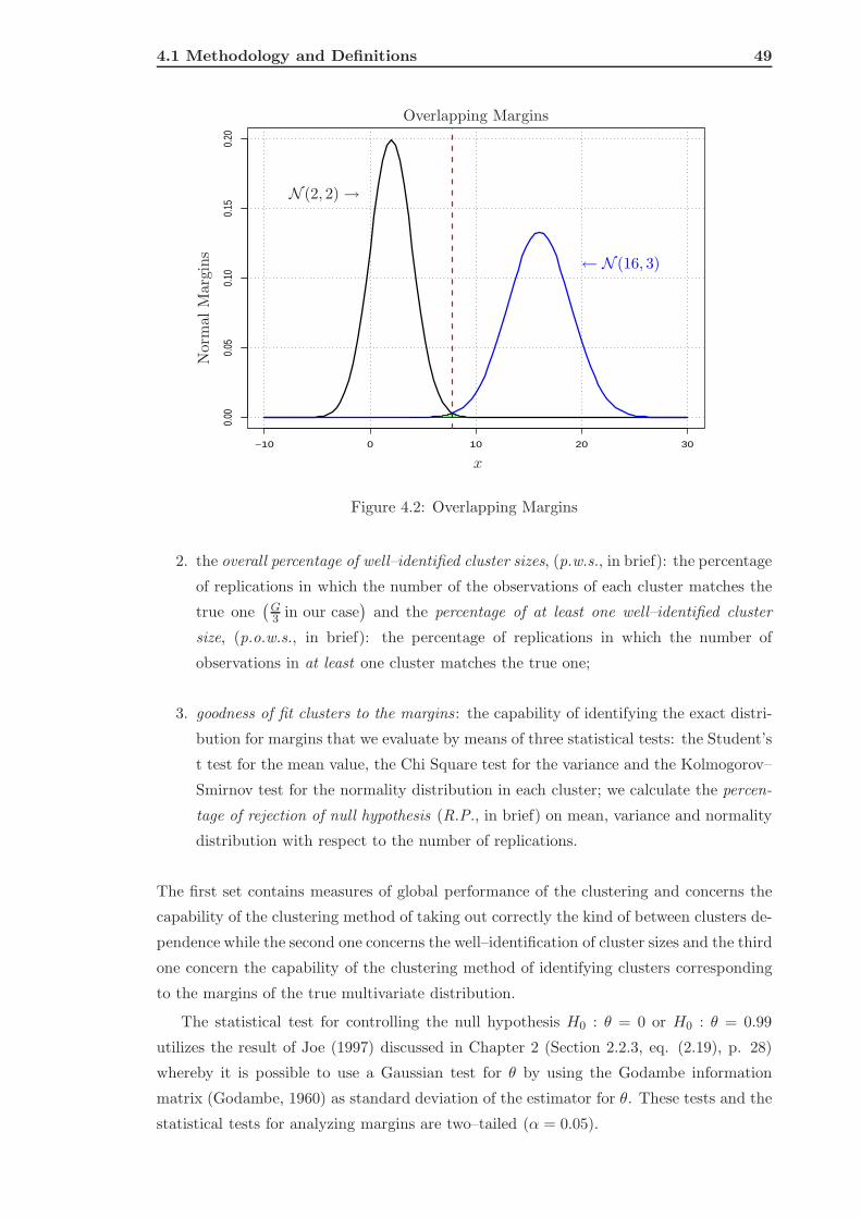
4.1 Methodology and Definitions 49
−10 0 10 20 30
0.00
0.05
0.10
0.15
0.20
Overlapping Margins
Nor
mal
Mar
gins
x
N (2, 2)→
← N (16, 3)
Figure 4.2: Overlapping Margins
2. the overall percentage of well–identified cluster sizes, (p.w.s., in brief): the percentage
of replications in which the number of the observations of each cluster matches the
true one(
G3 in our case
)
and the percentage of at least one well–identified cluster
size, (p.o.w.s., in brief): the percentage of replications in which the number of
observations in at least one cluster matches the true one;
3. goodness of fit clusters to the margins: the capability of identifying the exact distri-
bution for margins that we evaluate by means of three statistical tests: the Student’s
t test for the mean value, the Chi Square test for the variance and the Kolmogorov–
Smirnov test for the normality distribution in each cluster; we calculate the percen-
tage of rejection of null hypothesis (R.P., in brief) on mean, variance and normality
distribution with respect to the number of replications.
The first set contains measures of global performance of the clustering and concerns the
capability of the clustering method of taking out correctly the kind of between clusters de-
pendence while the second one concerns the well–identification of cluster sizes and the third
one concern the capability of the clustering method of identifying clusters corresponding
to the margins of the true multivariate distribution.
The statistical test for controlling the null hypothesis H0 : θ = 0 or H0 : θ = 0.99
utilizes the result of Joe (1997) discussed in Chapter 2 (Section 2.2.3, eq. (2.19), p. 28)
whereby it is possible to use a Gaussian test for θ by using the Godambe information
matrix (Godambe, 1960) as standard deviation of the estimator for θ. These tests and the
statistical tests for analyzing margins are two–tailed (α = 0.05).

50 Simulation Study
The good performance of a clustering technique lies on (1) the proximity of the esti-
mation of θ after simulation, that is, the mean value calculated on the total number of
simulations, that we indicate by θ∗, to the theoretical value and on a low percentage of
rejection of H0 about θ, (2) the proximity of the overall percentage of well–identified clus-
ter sizes and (3) the exact identification of the probability function of the margins, that
is on a low percentage of rejection of the null hypothesis on mean, variance and Gaussian
distribution for each identified cluster. Our attention essentially focus mainly on the first
set of measures of performance. Of course, this is not sufficient for evaluating the overall
performance since, as it will be possible to understand later, we can obtain (θ − θ∗) ≃ 0
even if we have clusters containing observations drawn from marginal probability function
different from the true one.
In summary, first we are going to check the first sets of measures and then we look at
the compliance between clusters and margins.
4.1.4 The Methods
In this section we present the rationale behind the use of copula functions as a means for
measuring the performance of clustering methods. The steps are as follows:
i) generate 3× n = G× S observations
x11 . . . x1S . . . x1n
x21 . . . x2S . . . x2n
x31 . . . x3S . . . x3n
from a trivariate distribution F by using a Gaussian copula C with dependence
parameter θ (see eq. (2.32), p. 31) with Gaussian margins F1, F2, F3:
F (x1, x2, x3) = C (F1(x1), F2(x2), F3(x3); θ) (4.4)
whose density is as follows
f(x1, x2, x3) = c (F1(x1), F2(x2), F3(x3); θ)
3∏
k=1
fk (xk;βk) (4.5)
and βk = (µk, σk) is the parameter vector of the k–th margin;
ii) arrange the observations in a G×S matrix (in which each row represents a gene and
each column an experimental condition) in a way such that the firstG
3rows contain
n observations generated by the first Gaussian margin, the secondG
3rows contain
the n observations generated by the second Gaussian margin and the thirdG
3rows
contain n observations generated by the third margin:
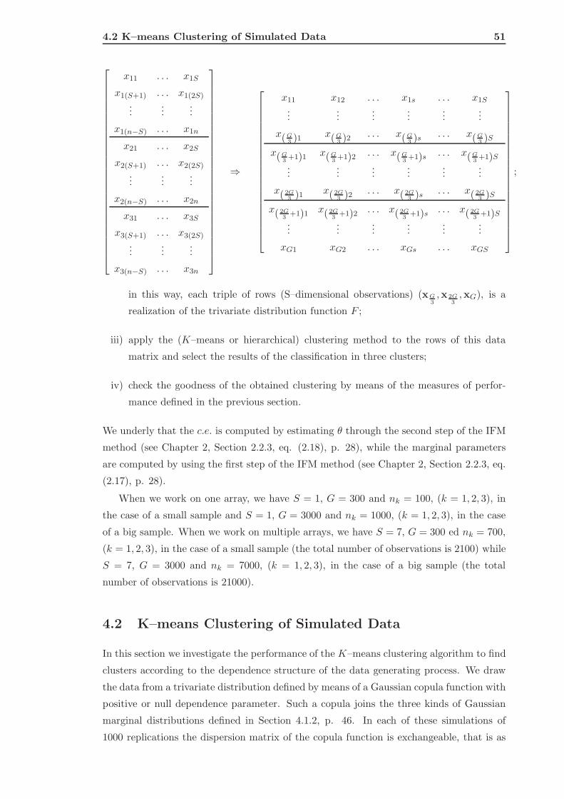
4.2 K–means Clustering of Simulated Data 51
x11 . . . x1S
x1(S+1) . . . x1(2S)
......
...
x1(n−S) . . . x1n
x21 . . . x2S
x2(S+1) . . . x2(2S)
......
...
x2(n−S) . . . x2n
x31 . . . x3S
x3(S+1) . . . x3(2S)
......
...
x3(n−S) . . . x3n
⇒
x11 x12 . . . x1s . . . x1S
......
......
......
x(G3 )1 x(G
3 )2 . . . x(G3 )s . . . x(G
3 )S
x(G3
+1)1 x(G3
+1)2 . . . x(G3
+1)s . . . x(G3
+1)S
......
......
......
x( 2G3 )1 x( 2G
3 )2 . . . x( 2G3 )s . . . x( 2G
3 )S
x( 2G3
+1)1 x( 2G3
+1)2 . . . x( 2G3
+1)s . . . x( 2G3
+1)S...
......
......
...
xG1 xG2 . . . xGs . . . xGS
;
in this way, each triple of rows (S–dimensional observations) (xG3,x 2G
3,xG), is a
realization of the trivariate distribution function F ;
iii) apply the (K–means or hierarchical) clustering method to the rows of this data
matrix and select the results of the classification in three clusters;
iv) check the goodness of the obtained clustering by means of the measures of perfor-
mance defined in the previous section.
We underly that the c.e. is computed by estimating θ through the second step of the IFM
method (see Chapter 2, Section 2.2.3, eq. (2.18), p. 28), while the marginal parameters
are computed by using the first step of the IFM method (see Chapter 2, Section 2.2.3, eq.
(2.17), p. 28).
When we work on one array, we have S = 1, G = 300 and nk = 100, (k = 1, 2, 3), in
the case of a small sample and S = 1, G = 3000 and nk = 1000, (k = 1, 2, 3), in the case
of a big sample. When we work on multiple arrays, we have S = 7, G = 300 ed nk = 700,
(k = 1, 2, 3), in the case of a small sample (the total number of observations is 2100) while
S = 7, G = 3000 and nk = 7000, (k = 1, 2, 3), in the case of a big sample (the total
number of observations is 21000).
4.2 K–means Clustering of Simulated Data
In this section we investigate the performance of the K–means clustering algorithm to find
clusters according to the dependence structure of the data generating process. We draw
the data from a trivariate distribution defined by means of a Gaussian copula function with
positive or null dependence parameter. Such a copula joins the three kinds of Gaussian
marginal distributions defined in Section 4.1.2, p. 46. In each of these simulations of
1000 replications the dispersion matrix of the copula function is exchangeable, that is as

52 Simulation Study
follows:
1 θ θ
θ 1 θ
θ θ 1
. (4.6)
In the following subsections we present the obtained results distinguishing between the
single array and the array matrix case. As mentioned above we compute the three set
of measures of performance and we put the results in two different tables: the first one
concerns the results of the computed measures about θ∗ and about the identified cluster
sizes and the second one contains the results of the statistical tests on the parameters and
the probability model of margins.
4.2.1 The Single Array Case
We remind that we call small a sample of 300 observations, (100 drawn from each one
margin) placed in a 300×1 matrix (consequently, the first 100 rows contain the observations
of the first margin, and so on) while we call big, a sample composed of 3000 observations
placed in a 3000 × 1 matrix (in this case, of course, the first 1000 rows of the matrix
contain the observations drawn from the first margin and so on).
For each one of the two considered values of the dependence parameter, we show the
results in two tables. As we have stressed, the first table presents results about the first
and the second set of performance measures, that is, about the analysis of dependence
between clusters and the evaluation about the cluster sizes, while the second one presents
the results about the third set of measures of performance, that is, the goodness of fit
clusters to margins. Notice that in the Tab. 4.1 the null hypothesis on the dependence
parameter is H0 : θ = 0 while in the Tab. 4.2 is H0 : θ = 0.99. Finally, we indicate in brief
by R.P. of Test the percentage of rejections of a null hypothesis H0 on the mean value,
the variance and the Gaussian distribution for each of the three clusters indicated by C1,
C2 and C3.
First of all, we note in Tab. 4.1 that the c.e. and the r.p. about the null hypothesis on
θ increase as soon as the margins become overlapping, irrespective of the sample size. A
similar trend have the p.w.s. and the p.o.w.s. that decrease as soon as the margins become
overlapping till to become zero in the case of nested margins. Even if the cluster effect and
the rejection percentage of the null hypothesis on θ are low, the p.w.s. is such that the
obtained clustering can not be deemed very good. As for the goodness of fit clusters to
margins (see Tab. 4.3), the performance of this clustering method is not good in general
(the rejection percentages are too high in each simulated setting) but it is better in the
case of well–separated and overlapping margins than in that of nested margins. On the
whole, the K–means method give us quite good results only in the case of small sample
and well–separated margin even if we do not consider it very satisfactory.
The obtained results for the maximum dependence case are similar to those observed in
the previous one both for the analysis of the performance about the clustering and for the
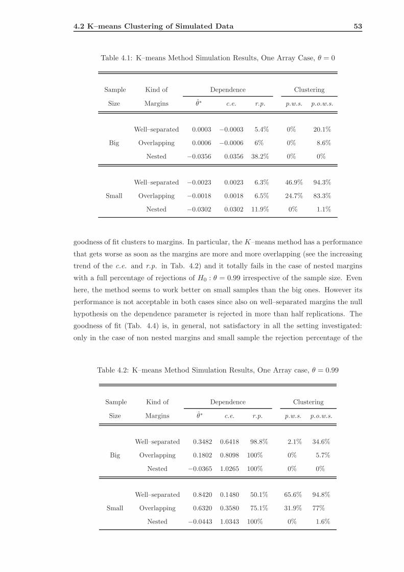
4.2 K–means Clustering of Simulated Data 53
Table 4.1: K–means Method Simulation Results, One Array Case, θ = 0
Sample Kind of Dependence Clustering
Size Margins θ∗ c.e. r.p. p.w.s. p.o.w.s.
Well–separated 0.0003 −0.0003 5.4% 0% 20.1%
Big Overlapping 0.0006 −0.0006 6% 0% 8.6%
Nested −0.0356 0.0356 38.2% 0% 0%
Well–separated −0.0023 0.0023 6.3% 46.9% 94.3%
Small Overlapping −0.0018 0.0018 6.5% 24.7% 83.3%
Nested −0.0302 0.0302 11.9% 0% 1.1%
goodness of fit clusters to margins. In particular, the K–means method has a performance
that gets worse as soon as the margins are more and more overlapping (see the increasing
trend of the c.e. and r.p. in Tab. 4.2) and it totally fails in the case of nested margins
with a full percentage of rejections of H0 : θ = 0.99 irrespective of the sample size. Even
here, the method seems to work better on small samples than the big ones. However its
performance is not acceptable in both cases since also on well–separated margins the null
hypothesis on the dependence parameter is rejected in more than half replications. The
goodness of fit (Tab. 4.4) is, in general, not satisfactory in all the setting investigated:
only in the case of non nested margins and small sample the rejection percentage of the
Table 4.2: K–means Method Simulation Results, One Array case, θ = 0.99
Sample Kind of Dependence Clustering
Size Margins θ∗ c.e. r.p. p.w.s. p.o.w.s.
Well–separated 0.3482 0.6418 98.8% 2.1% 34.6%
Big Overlapping 0.1802 0.8098 100% 0% 5.7%
Nested −0.0365 1.0265 100% 0% 0%
Well–separated 0.8420 0.1480 50.1% 65.6% 94.8%
Small Overlapping 0.6320 0.3580 75.1% 31.9% 77%
Nested −0.0443 1.0343 100% 0% 1.6%
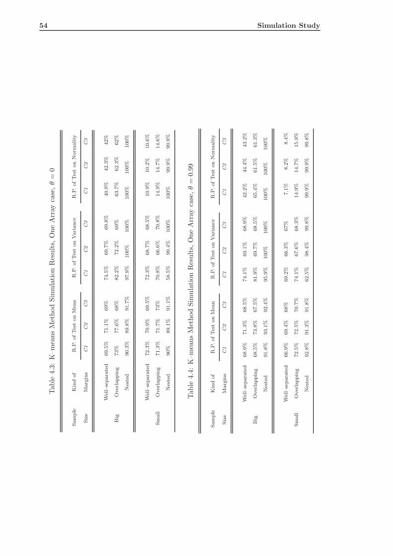
54 Simulation Study
Tab
le4.
3:K
–mea
ns
Met
hod
Sim
ula
tion
Res
ults,
One
Arr
ayca
se,θ
=0
Sam
ple
Kin
dof
R.P
.ofTes
ton
Mea
nR
.P.ofTes
ton
Vari
ance
R.P
.ofTes
ton
Norm
ality
Siz
eM
arg
ins
C1
C2
C3
C1
C2
C3
C1
C2
C3
Wel
l–se
para
ted
69.5
%71.1
%69%
74.5
%69.7
%69.8
%40.9
%42.3
%42%
Big
Over
lappin
g73%
77.6
%68%
82.2
%72.2
%69%
63.7
%62.3
%62%
Nes
ted
90.3
%89.8
%91.7
%97.9
%100%
100%
100%
100%
100%
Wel
l–se
para
ted
72.3
%70.9
%69.5
%72.3
%68.7
%68.5
%10.9
%10.2
%10.6
%
Sm
all
Over
lappin
g71.3
%71.7
%73%
70.8
%66.6
%70.8
%14.9
%14.7
%14.6
%
Nes
ted
90%
89.1
%91.1
%58.5
%99.4
%100%
100%
99.9
%99.9
%
Tab
le4.
4:K
–mea
ns
Met
hod
Sim
ula
tion
Res
ults,
One
Arr
ayca
se,θ
=0.
99
Sam
ple
Kin
dof
R.P
.ofTes
ton
Mea
nR
.P.ofTes
ton
Vari
ance
R.P
.ofTes
ton
Norm
ality
Siz
eM
arg
ins
C1
C2
C3
C1
C2
C3
C1
C2
C3
Wel
l–se
para
ted
68.9
%71.3
%68.5
%74.1
%69.1
%68.9
%42.2
%44.4
%43.2
%
Big
Over
lappin
g68.5
%73.8
%67.5
%81.9
%69.7
%68.5
%65.4
%61.5
%61.3
%
Nes
ted
91.8
%93.1
%92.4
%95.9
%100%
100%
100%
100%
100%
Wel
l–se
para
ted
66.9
%69.4
%68%
69.2
%66.3
%67%
7.1
%8.2
%8.4
%
Sm
all
Over
lappin
g72.5
%72.5
%70.7
%74.1
%67.6
%68.3
%14.9
%14.7
%15.9
%
Nes
ted
92.8
%91.3
%91.8
%62.5
%98.4
%99.8
%99.9
%99.9
%99.8
%

4.2 K–means Clustering of Simulated Data 55
hypothesis on Gaussian distribution is low.
The performance of K–means method turns out to be not good in each investigated
case except for the case of independence between well–separated margins and small samples
in which just in the 6.3% of the replications the null hypothesis on θ is rejected and in
almost 50% of replications the K–means method identifies the true number of observations
in each cluster. In all remaining settings it does not work satisfactorily.
4.2.2 The Array Matrix Case
In this second set of simulations we call small a sample of 2100 observation (700 from each
margin) placed in a 300× 7 matrix (the first 100 rows contain the observations of the first
margin, and so on) and big a sample composed of 21000 observations placed in a 3000× 7
matrix (in this case, of course, the first 1000 rows of the matrix contain the observations
drawn from the first margin and so on). In order to compare the already obtained results
with the new ones we choose the same number of rows and columns of the previous set of
simulations. Notice that the remarks about the notation of the columns of the following
tables are the same of the previous section.
Table 4.5: K–means Method Simulation Results, Array Matrix Case, θ = 0
Sample Kind of Dependence Clustering
Size Margins θ∗ c.e. r.p. p.w.s. p.o.w.s.
Well–separated −0.0079 0.0079 27% 73.6% 73.6%
Big Overlapping −0.0086 0.0086 29.3% 71.2% 71.2%
Nested −0.0356 0.0356 38.2% 0% 0%
Well–separated −0.0104 0.0104 9.5% 72% 72%
Small Overlapping −0.0102 0.0102 6.6% 74.5% 74.5%
Nested −0.0905 0.0905 91.8% 0.2% 6.8%
The K–means method totally fails in the case of independent nested margins, especially in
the case of small sample with a r.p. equal to 91.8% and p.w.s. equal to 0.2% (see Tab. 4.5).
The cluster effect and the percentage of rejections of null hypothesis on the dependence
parameter increase with the degree of overlap of margins and contemporaneously the p.w.s.
and the p.o.w.s. decrease till to become zero (especially in the case of big sample). In
the whole, the K–means seems to work better on small samples when the margins are not
nested. The statistical test computed for each cluster reveals a good identification of the
probability model for margins when the margins are not nested irrespective of the sample
size (see Tab. 4.7) even if the percentage of rejections for the mean and the variance values

56 Simulation Study
Table 4.6: K–means Method Simulation Results, Array Matrix Case, θ = 0.99
Sample Kind of Dependence Clustering
Size Margins θ∗ c.e. r.p. p.w.s. p.o.w.s.
Well–separated 0.7410 0.2490 46.9% 75.6% 75.6%
Big Overlapping 0.7522 0.2378 43% 76.7% 76.7%
Nested −0.0795 1.0695 100% 0% 1.6%
Well–separated 0.7131 0.2769 46.6% 72.9% 72.9%
Small Overlapping 0.7424 0.2476 43.1% 75.8% 75.8%
Nested −0.1033 1.0933 100% 0% 5.8%
reveal, on the whole, a not acceptable goodness of fit clusters to margins. Comparing these
results with those in Tab. 4.1 we can state that the K–means works better in the matrix
array case when the sample is small and the margins are not nested.
In the maximum dependence case (see Tab. 4.6), K–means method totally fails in the
case of nested margins with the c.e. equal to 100% and the r.p. equal to 0% irrespective of
the sample size. Its performance in the case of well–separated and overlapping margins is
similarly not satisfactory because of a too high r.p. This remark is confirmed by the results
about the statistical tests computed for each cluster (Tab. 4.8). As in the previous case,
the K–means method appears able to identify the true probability model for margins in the
not nested margins cases but if fails in the nested margins ones. In general, its performance
is not satisfactory and it is worse with respect to that obtained in the independence case
(comparing tables 4.5 and 4.6).
Summarizing, K–means method seems do not work in a satisfactory way in each inves-
tigated setting. Both in the case of one array and matrix array, it works better in the case
of independence. In this case, as regards the cluster effect and the percentage of rejection
of null hypothesis on the dependence parameter it works better on one array when the
margins are well–separated whereas for the percentage of well–identified cluster sizes it
seems to work better in the matrix array case. The best case is that of small matrix array
and independence between not nested margins even if, for this setting, the goodness of
fitting margins to clusters is not very satisfactory. On the whole, the performance of the
K–means method gets worse as long as the marginal distributions are not well–divided
both in the case of maximum positive dependence and in the case of independence between
clusters and it totally fails in the nested margins case.
In conclusion, we can state that the K–means method is able to find clusters according
to the data generating process and we can use the copula function to investigate it if and
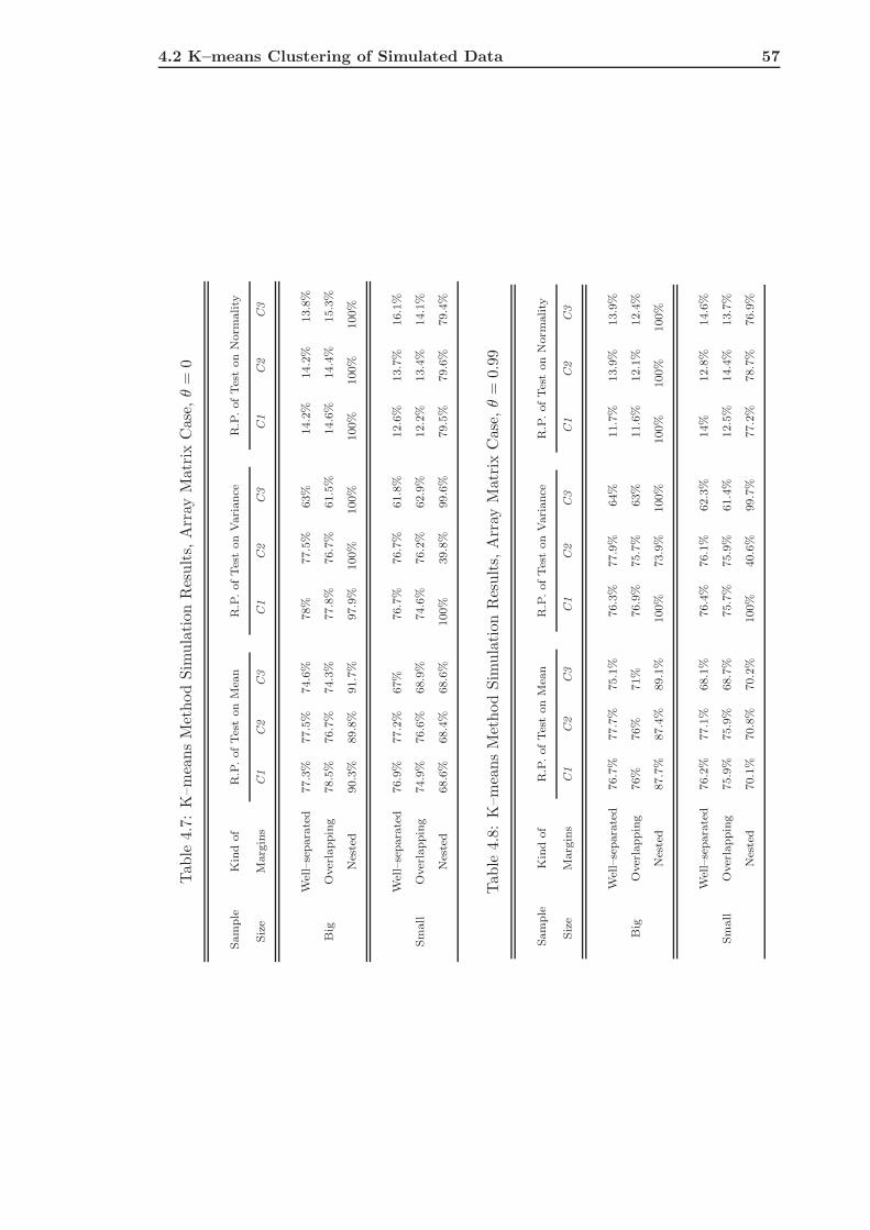
4.2 K–means Clustering of Simulated Data 57
Tab
le4.
7:K
–mea
ns
Met
hod
Sim
ula
tion
Res
ults,
Arr
ayM
atri
xC
ase,
θ=
0
Sam
ple
Kin
dof
R.P
.ofTes
ton
Mea
nR
.P.ofTes
ton
Vari
ance
R.P
.ofTes
ton
Norm
ality
Siz
eM
arg
ins
C1
C2
C3
C1
C2
C3
C1
C2
C3
Wel
l–se
para
ted
77.3
%77.5
%74.6
%78%
77.5
%63%
14.2
%14.2
%13.8
%
Big
Over
lappin
g78.5
%76.7
%74.3
%77.8
%76.7
%61.5
%14.6
%14.4
%15.3
%
Nes
ted
90.3
%89.8
%91.7
%97.9
%100%
100%
100%
100%
100%
Wel
l–se
para
ted
76.9
%77.2
%67%
76.7
%76.7
%61.8
%12.6
%13.7
%16.1
%
Sm
all
Over
lappin
g74.9
%76.6
%68.9
%74.6
%76.2
%62.9
%12.2
%13.4
%14.1
%
Nes
ted
68.6
%68.4
%68.6
%100%
39.8
%99.6
%79.5
%79.6
%79.4
%
Tab
le4.
8:K
–mea
ns
Met
hod
Sim
ula
tion
Res
ults,
Arr
ayM
atri
xC
ase,
θ=
0.99
Sam
ple
Kin
dof
R.P
.ofTes
ton
Mea
nR
.P.ofTes
ton
Vari
ance
R.P
.ofTes
ton
Norm
ality
Siz
eM
arg
ins
C1
C2
C3
C1
C2
C3
C1
C2
C3
Wel
l–se
para
ted
76.7
%77.7
%75.1
%76.3
%77.9
%64%
11.7
%13.9
%13.9
%
Big
Over
lappin
g76%
76%
71%
76.9
%75.7
%63%
11.6
%12.1
%12.4
%
Nes
ted
87.7
%87.4
%89.1
%100%
73.9
%100%
100%
100%
100%
Wel
l–se
para
ted
76.2
%77.1
%68.1
%76.4
%76.1
%62.3
%14%
12.8
%14.6
%
Sm
all
Over
lappin
g75.9
%75.9
%68.7
%75.7
%75.9
%61.4
%12.5
%14.4
%13.7
%
Nes
ted
70.1
%70.8
%70.2
%100%
40.6
%99.7
%77.2
%78.7
%76.9
%

58 Simulation Study
only if the margins are independent and not nested and they generate a small matrix
array of data.
4.3 Hierarchical Clustering of Simulated Data
In this section we study the capability of the hierarchical clustering method to find clusters
according to the data generator process. The simulations settings are the same as those
described in the previous sections.
4.3.1 The Single Array Case
Here summarize the simulations regarding the hierarchical clustering method applied to
one array dividing the results in two tables as we performed to analyze the performance
of the K–means method.
Table 4.9: Hierarchical Clustering Simulation Results, One Array Case, θ = 0
Sample Kind of Dependence Clustering
Size Margins θ∗ c.e. r.p. p.w.s. p.o.w.s.
Well–separated 0.0008 −0.0008 5.2% 2.5% 39%
Big Overlapping 0.0012 −0.0012 5.4% 0.8% 27.2%
Nested −0.0154 0.0154 20.1% 0% 0%
Well–separated 0.0011 −0.0011 6.1% 52.8% 94.8%
Small Overlapping 0.0012 −0.0012 6.1% 32.6% 89.7%
Nested −0.0234 0.0234 24.9% 0% 0%
In the case of independence (tables 4.9 and 4.11), we note that the performance of
the hierarchical clustering method gets worse as long as the margins are more and more
overlapping. As for c.e. and r.p. the method appears to be quite good irrespective of the
sample size and the kind of margins whereas as for the p.w.s. and the p.o.w.s. it totally
fails in each analyzed case except for the small sample drawn from well–separated margins.
On the whole, it works better in the small sample case then in the big one. As for the
performance about the goodness of fit clusters to margins, we note that it works quite
well in the case of non nested margins. However, it gets worse as long as they become
more and more overlapping. The best performance appears for the case of a small sample
drawn form well–separated margins.
Straightaway we note that the performance of this clustering method in the maximum
dependence case (tables 4.10 and 4.12) goes from bad to worse as long as the margins

4.3 Hierarchical Clustering of Simulated Data 59
Table 4.10: Hierarchical Clustering Simulation Results, One Array Case, θ = 0.99
Sample Kind of Dependence Clustering
Size Margins θ∗ c.e. r.p. p.w.s. p.o.w.s.
Well–separated 0.2909 0.6991 96% 7.7% 44.9%
Big Overlapping 0.1610 0.8290 99.8% 1.5% 26.1%
Nested −0.0180 0.9720 90.3% 0% 0%
Well–separated 0.7772 0.2128 54.7% 62.7% 92.9%
Small Overlapping 0.6794 0.3106 67.8% 42.5% 90.9%
Nested −0.0464 1.0364 85.9% 0% 0%
become more and more overlapping. The failure of the hierarchical method in the case of
nested margins is total in the sense that it embraces c.e., r.p and p.w.s. (see Tab. 4.10).
The performance is better in the small sample case but the high percentage of rejections
of the null hypothesis on the dependence parameter leads us to not accept this method as
a procedure to analyze the dependence structure underlying the data. At the same time,
the goodness of fit clusters to margins is quite good in not nested margins cases and it is
better in the case of small samples.
Comparing the obtained results in the two different dependence settings, we can state
that the hierarchical clustering method works better on small sample and in this case,
it works better in the independence case. As for the cluster effect and the r.p. it is
satisfactory irrespective of the kind of margins (see Tab. 4.9) but as soon the p.w.s. and
the rejection percentages of the tests on margins are observed, the not nested margins
cases become not acceptable. In conclusion, we may state that this method works quite
well just in the case of independence between well–separated margins and small sample.
4.3.2 The Array Matrix Case
Here summarize the simulations on hierarchical clustering analysis applied to a microarray
matrix consisted of seven columns. For the definition of sample size and kind of margins
we remind to the previously sections.
The hierarchical clustering method works well both on well–separated and overlapping
margins presenting a low cluster effect and a full percentage of well–identified cluster sizes
but it suddenly totally fails on nested margins as regards the p.w.s. and it gets worse as
concerning the c.e. (see Tab. 4.13). The performance on the margins (see Tab. 4.15)
is similar to that about the dependence and the clustering. The whole performance of
the hierarchical method changes in the extreme case of nested margins while there are

60 Simulation Study
Tab
le4.
11:
Hie
rarc
hic
alC
lust
erin
gSim
ula
tion
Res
ults,
One
Arr
ayC
ase,
θ=
0
Sam
ple
Kin
dof
R.P
.ofTes
ton
Mea
nR
.P.ofTes
ton
Vari
ance
R.P
.ofTes
ton
Norm
ality
Siz
eM
arg
ins
C1
C2
C3
C1
C2
C3
C1
C2
C3
Wel
l–se
para
ted
10.5
%15.2
%9.8
%22.1
%27.9
%15.4
%32.3
%51.4
%29%
Big
Over
lappin
g22.8
%24.6
%8.5
%34.6
%37.8
%14.4
%46.8
%64.5
%27%
Nes
ted
74%
98.7
%82.4
%97.4
%95.5
%70%
99.9
%91.1
%52.9
%
Wel
l-se
para
ted
6.8
%8%
6%
11.1
%12.2
%7.5
%13.8
%13.3
%6.1
%
Sm
all
Over
lappin
g9.6
%10.3
%5.3
%17.6
%14%
6.4
%17.4
%17.4
%6.3
%
Nes
ted
58.1
%97.1
%75.8
%77%
88.1
%57.1
%83.7
%68.5
%25.4
%
Tab
le4.
12:
Hie
rarc
hic
alC
lust
erin
gSim
ula
tion
Res
ults,
One
Arr
ayC
ase,
θ=
0.99
Sam
ple
Kin
dof
R.P
.ofTes
ton
Mea
nR
.P.ofTes
ton
Vari
ance
R.P
.ofTes
ton
Norm
ality
Siz
eM
arg
ins
C1
C2
C3
C1
C2
C3
C1
C2
C3
Wel
l–se
para
ted
11.4
%15.3
%9.4
%23.4
%24.1
%14.1
%35.1
%49.9
%27.2
%
Big
Over
lappin
g28.1
%29.8
%9.8
%38%
40.7
%14.1
%50.7
%66.6
%29%
Nes
ted
76.5
%98.8
%82.8
%97.8
%96.1
%72.9
%100%
94%
55%
Wel
l–se
para
ted
6.6
%8.3
%6.5
%9.8
%9.2
%5.9
%13.3
%15.2
%6.9
%
Sm
all
Over
lappin
g10.2
%12.1
%7.1
%16.3
%13%
5.3
%16.3
%16.7
%7.2
%
Nes
ted
65.2
%96.6
%76.5
%79.1
%84.5
%57.1
%84.3
%71.9
%24.7
%

4.3 Hierarchical Clustering of Simulated Data 61
Table 4.13: Hierarchical Clustering Simulation Results, Array Matrix Case, θ = 0
Sample Kind of Dependence Clustering
Size Margins θ∗ c.e. r.p. p.w.s. p.o.w.s.
Well–separated −0.0002 0.0002 5.9% 100% 100%
Big Overlapping 0.00004 −0.00004 4.7% 100% 100%
Nested 0.0003 −0.0003 20.8% 0% 0%
Well–separated −0.0007 0.0007 6% 100% 100%
Small Overlapping −0.0007 0.0007 5.3% 100% 100%
Nested −0.0275 0.0275 19.2% 0% 0%
not important differences between the case of well–separated and overlapping margins in
which its performance appear satisfactory.
The performance of the hierarchical clustering in the maximum dependence case (Tab.
4.14) is similar to that in the dependence case: the method works quite well on well–
separated and overlapping margins. As regards the nested margins case, this method
totally fails irrespective of the sample size. The performance on the margins is coherent
with the results just discussed (see Tab. 4.16).
Summarizing, the only factor that affects the performance of this clustering method
is the degree of overlap of margins. When margins are well–separated as well as they
Table 4.14: Hierarchical Clustering Simulation Results, Array Matrix Case, θ = 0.99
Sample Kind of Dependence Clustering
Size Margins θ∗ c.e. r.p. p.w.s. p.o.w.s.
Well–separated 0.9899 0.0001 30.6% 100% 100%
Big Overlapping 0.9899 0.0001 30.3% 100% 100%
Nested −0.0108 1.0008 98.3% 0% 0%
Well–separated 0.9899 0.00001 28.8% 100% 100%
Small Overlapping 0.99 0 29.2% 100% 100%
Nested −0.0074 0.9974 97.8% 0% 0%
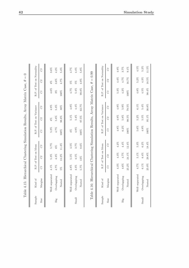
62 Simulation Study
Tab
le4.
15:
Hie
rarc
hic
alC
lust
erin
gSim
ula
tion
Res
ults,
Arr
ayM
atri
xC
ase,
θ=
0
Sam
ple
Kin
dof
R.P
.ofTes
ton
Mea
nR
.P.ofTes
ton
Vari
ance
R.P
.ofTes
ton
Norm
ality
Siz
eM
arg
ins
C1
C2
C3
C1
C2
C3
C1
C2
C3
Wel
l–se
para
ted
4.1
%5.3
%5.7
%5.2
%4%
4.9
%4.6
%4%
3.6
%
Big
Over
lappin
g4.7
%4.3
%6%
4.7
%5.8
%5.3
%3%
3.6
%4.2
%
Nes
ted
5%
13.2
%11.4
%100%
98.8
%88%
100%
4.7
%5.4
%
Wel
l–se
para
ted
4.8
%5.5
%4.5
%4%
5.1
%4.8
%4.7
%5%
4.7
%
Sm
all
Over
lappin
g4.3
%4.5
%3.7
%4.9
%5.4
%4.4
%5.4
%5%
4.4
%
Nes
ted
5.7
%13%
8.6
%100%
97.5
%63.7
%99.8
%4.9
%5.8
%
Tab
le4.
16:
Hie
rarc
hic
alC
lust
erin
gSim
ula
tion
Res
ults,
Arr
ayM
atri
xC
ase,
θ=
0.99
Sam
ple
Kin
dof
R.P
.ofTes
ton
Mea
nR
.P.ofTes
ton
Vari
ance
R.P
.ofTes
ton
Norm
ality
Siz
eM
arg
ins
C1
C2
C3
C1
C2
C3
C1
C2
C3
Wel
l–se
para
ted
4.3
%4.3
%4.2
%4.8
%4.9
%4.9
%5.3
%4.4
%4.9
%
Big
Over
lappin
g4.6
%4.7
%4.4
%6.2
%5.8
%5.9
%4.2
%4.7
%3.7
%
Nes
ted
25.2
%24.1
%12.4
%100%
98.5
%79.5
%100%
16.7
%9.1
%
Wel
l–se
para
ted
4.7
%5.1
%5.3
%5.6
%5.2
%6.1
%4.8
%5.2
%4.5
%
Sm
all
Over
lappin
g6.1
%6.4
%6.2
%4.9
%5.5
%5.4
%4.5
%4.3
%5.2
%
Nes
ted
25.9
%29.8
%18.4
%100%
95.1
%30.8
%98.4
%18.5
%11.5
%

4.4 Discussion 63
are overlapping, the hierarchical clustering method is quite able to find clusters according
to the dependence structure and each cluster fits a margin in a satisfactory way. When
the margins are nested, this clustering method fails completely. Clearly, the threshold
between the success and the flop of the hierarchical clustering method performance needs
to be investigated. We may argue it depends on the particular values of the marginal
parameters, in particular on the variance value, and on the heaviness of the tails of these
distributions.
Comparing these results to those obtained in the independence case, we note that the
method works better in the independence case than in the maximum dependence case
both for the c.e. and for the r.p. about H0 on θ that are lower in the former than in the
latter case. Moreover, the r.p. is almost equal to 100% in the maximum dependence case
and nested margins (vs ≈ 20% in the independence case). Instead, as regards the p.w.s.,
the performance is perfectly the same in the two cases analyzed, θ = 0 and θ = 0.99. In
conclusion, we may state that the hierarchical method has the best performance in the
case of independent not nested margins.
4.4 Discussion
In this section we compare the two clustering methods summarizing the situations in which
it may be convenient to prefer one above the other in the applications.
4.4.1 Remark on the Two Clustering Methods
In general, we have found that when we work with data generated from a multivariate
distribution with independent margins the K–means method works according to the kind
of the dependence if and only if the marginal probability functions are not nested (prefer-
ably well–separated) and the sample is small. A possible explanation of this result, might
be that the small sample case reduces the possibility to draw from two different margins
two values close to each other. Moreover, in the settings above explained, the K–means
method works better if it is applied to a matrix array, that is, the performance of the
K–means method increases with the dimension of the observational space.
The hierarchical clustering method works well in the array matrix case of independent
not nested margins. The c.e. and the r.p. are very low and the p.w.s. is maximum. As we
have stated it is difficult to find from these results a general threshold between the success
and the failure of this clustering method because of the particular parameter values of
margins. Still, we think that some results are promising and deserve further investigations.
As it was possible to observe in previous sections, the hierarchical clustering method has
contrasting performance if applied to one or more than one array. When it is applied
to only one array it works better on independent well–separated margins that generate
small sample whereas when applied to a matrix array it works quite well irrespective of
the sample size even if its performance is again better in the independence case. Finally,

64 Simulation Study
we have observed that this method totally fails if applied to nested margins.
In the next section we are going to discuss the performance of the two investigated
clustering methods.
4.4.2 K–means vs Hierarchical Clustering
When applied to only one array, the two clustering methods have similar performances.
Both the K–means and the hierarchical methods work quite well just in the case of inde-
pendent, well–separated margins and small sample (see tables 4.1 and 4.9). The cluster
effect and the percentage of rejections of the null hypothesis on the dependence parameter
are very low (≈ 6%) even if the p.w.s. is close to 50% for both methods.
When applied to a matrix array, the hierarchical method seems to outperform the
K–means method. Again, they both have a good performance in the independence case;
in particular, in such a case the hierarchical clustering has a satisfactory performance
irrespective of the sample size (see Tab. 4.13) whereas the K–means method works better
on small samples rather than on big ones (see Tab. 4.5). Moreover, on an array matrix,
the hierarchical method seems to be able to identify the true dependence structure if the
margins are not nested and preferably independent.
Comparing the performance of the K–means method with that of hierarchical cluster-
ing method in the two cases in which they both have a good performance (well–separated
or overlapping independent margins on array matrix case), it is clear that the hierarchical
method works better than K–means since the former has p.w.s. = 100% vs the latter
that has p.w.s. ≈ 70% even if both have very similar c.e. (at least in the small sample
case). As for the goodness of fit clusters to margins, hierarchical method appears to work
better than the K–means method. In the nested margin case, both the hierarchical and
the K–means methods fail.
Finally, for both the two clustering methods the degree of overlap of margins determines
a drop of their performance. We may argue that as margins tend to overlap increasingly
we likely have observations with low Euclidean distance but drawn from different distri-
butions, observations that the clustering algorithm will assign to the same cluster and fail
to reproduce adequately the dependence structure of the data.
On the whole, the performance of both these two methods is not satisfactory to achieve
the purpose of finding a procedure to separate genes in light of the dependence relationship
between their mRNA quantity. However, in the next section we give some indications for
a better use of these two clustering methods for the empirical applications.
4.4.3 Relevance to Empirical Applications
When we need to analyze a microarray data matrix, we should follow this outline:
1. check the number of observations (rows) and experimental conditions (columns);
2. choose the kind of clustering method between K–means and hierarchical methods;

4.4 Discussion 65
3. apply the method chosen at step 2. to the rows matrix;
4. analyze clusters and infer a probability model for each one of them (estimate pa-
rameters trough equation (2.17) (Chapter 2, p. 28);
5. estimate copula function on identified clusters trough the second step of IFM in eq.
(2.18) (Chapter 2, p. 28);
6. evaluate if the estimated dependence parameter value can be accepted.
How can we know if the clusters reflect the true underlying? We give two different guide-
lines for empirical applications based on the simulation results discussed up to now. When
we work on one array, the practical conclusion is the same for the two clustering methods
investigated:
1. if the sample size is small we can apply one of the two clustering methods and
2. after clustering, we can accept the result if and only if the marginal probability
functions are well–separated and θ does not differs significantly from zero
3. otherwise the use of these two clustering methods is not advised.
When we work on a whole array data matrix,
1. we can apply the K–means method if the sample size is small and
2. after clustering, we can accept the results if and only if the margins are not nested
and θ does not differs significantly from zero.
As regards the hierarchical method, the small sample size requirement is not needed if
we work on a whole matrix data. Obviously these conclusions are drawn from the simu-
lation study performed so that they need to be validated and substantiated with further
investigations.


Chapter 5
A copula–based clustering
algorithm
In this chapter we present in detail a new clustering algorithm based on copula func-
tions (‘CoClust’ in brief). The main idea lies in the use of copula functions as a tool for
investigating the dependence relationship between gene expressions (or experimental con-
ditions) and for finding clusters of genes (or experimental conditions) according to their
dependence structure.
We test the CoClust on simulated data for different situations and dependence settings.
This new algorithm allows to overcome the limits of the two clustering methods highlighted
in the simulation study in Chapter 4, p. 45. Finally, we compare the CoClust with the
model–based clustering (see Chapter 1, Section 1.2.3, p. 13).
5.1 A New Clustering Algorithm
In this section we describe the procedure of the clustering algorithm and focus on both the
statistical aspects and the criterion for allocating the observations to clusters. In the last
subsection we describe the output of the main R code (see Appendix A, p. 117) written
for the CoClust.
5.1.1 A Copula–based Clustering Algorithm
The results of the simulation study in Chapter 4 (p. 45) pose important questions about
the use of cluster analysis for dependent observations. In microarray experiments we have
thousands of gene expressions observed under different experimental conditions. Genes
are observed by means of the quantity of mRNA they produce. Such a quantity depends
on both biological function of genes themselves and the biological process in which they
are involved. These genes are related to each other and our purpose is to find a procedure
capable of grouping them according to their dependence relationship.
The clustering algorithm we propose works directly on the observed (G×S) data matrix
(3.1) in Chapter 3, p. 38 (like the K–means algorithm and the model–based clustering
67
68 A copula–based clustering algorithm
presented in Chapter 1, Sections 1.2.1, p. 9 and 1.2.3, p. 13) and not on the proximity
matrix (like the hierarchical method in Chapter 1, Section 1.2.2, p. 11) while it does not
require the number of clusters to be specified a priori (like the hierarchical and model–
based clustering and differently from the K–means algorithm). Notice that the meaning
of the terms ‘margin’ and ‘cluster’ are interchangeable since we think each cluster, that is
each subset of rows of a microarray data matrix, as a sample drawn from the same margin.
Applying the CoClust to the genes (rows) means that each observation in each cluster is
an S–dimensional vector drawn from a univariate probability function.
The copula–based clustering algorithm (CoClust, in brief) consists of the following
steps:
1. For k = 2, 3, . . . ,K estimate a k–dimensional copula function for each possible k–
plet of observations (rows of data matrix or gene expressions), that is, estimate
CG,k =
(
G
k
)
=G!
k!(G − k)!copula functions and compute the maximum log–likelihood
of each one of them;
2. Select the value of k and the k–plet the maximizes the log–likelihood copula function
computed at step 1.); as long as a dimension k of copula is chosen, k clusters each
one containing one observation (one gene expression or, equally, an S–dimensional
vector of values) will been identified;
3. Once chosen k, estimate DG−k,k =(G− k)!
(G− 2k)!=
k−1∏
j=0
(G−k−j) k–dimensional copulas
by using the k–plet already selected at step 2.) and a new k–plet of rows data
matrix; this means that the algorithm estimates each copula function by using 2S
observations for each one of marginal distribution function of each copula function:
the first observation coming from the first S–dimensional observations selected at
step 2.) while the second observation varies between the remaining (G−k) rows data
matrix. Notice that hereafter the order of the k–plet of observations candidate for
the selection is important ;
4. Select the new k–plet that once put together with the existing ones maximize the
log–likelihood computed at step 3.);
5. Iterate steps 3.) and 4.) estimating as many copulas as are the dispositions of the
remaining genes by using the observations already clustered and a new k–plet chosen
between the remaining genes for each margin (G−k, G−2k, and so on); the iteration
continues until each row of data matrix is assigned to a cluster.
Notice that it is possible to select the best result by comparing each solution directly
by means of the maximized log–likelihood function of the copula because of the same
sample size and the same number of estimated parameters. This is admitted both for
step 1.) and for step 3.). Indeed, in the first case the algorithm compares the value of the
maximum log–likelihood copula function for each value of k and, later, the selected values
5.1 A New Clustering Algorithm 69
for fixed k having always just an S–dimensional observation in each cluster. In the latter
case the algorithm chooses the clusters number so that, at each iteration, the number of
observations for each copula is the same
(
from 2 toG
k
)
. In both cases the number of
estimated parameters is the same because of the use of the IFM estimation method: at
each computation of the log–likelihood copula function the marginal parameters have been
already estimated and they are considered constant. We hark on it in the next section.
5.1.2 Copula–based Split up Rule
In this section we discuss from a statistical point of view the so–called copula log–likelihood–
based split up rule, (COSUR, in brief) used in the procedure of the CoClust described in
the previous section.
The basic idea is that the COSUR rule separates two observations (in the case of
two–dimensional copula) allocating them in two different clusters that are assumed to
be realizations of two different (marginal) random variables for which the maximized log–
likelihood copula function is maximum. In order to estimate copula functions the algorithm
uses the IFM estimation method (see Chapter 2, Section 2.2.3, p. 28) and, consequently,
employs the parameters estimates βgkfor each gk–th margin, with k = 1, 2, . . . ,K and K
the number of margins (or clusters), estimated in the first step of IFM estimation method.
The copula log–likelihood–based split up rule involves only the dependence parameter and,
consequently, involves only the second step of the IFM estimation method.
At the first step of the procedure described in previous subsection the following value
is computed:
max{
lxgi1...xgik
(
θ2IFM
)
, ∀ (gi1 , . . . , gik′ , . . . , gik) ∈ {1, 2, . . . , G}, with k 6= k′ ∀ k, k′}
=
= max
{
maxθ2∈Θ
S∑
s=1
log c[
Fg1
(
Xg1s; βg1
)
, . . . , Fgk′
(
Xgk′s; βgk′
)
, . . . (5.1)
. . . , Fgk
(
Xgks; βgk
)
; θ2
]
; ∀ (gi1 , . . . , gik′ , . . . , gik) ∈ {1, 2, . . . , G}, with k 6= k′ ∀ k, k′}
where l(θ2IFM) is the maximized log–likelihood function of a copula and the generic
vector βgkcontains the parameters of the gk–th margin estimated by using equation
(2.17) (Chapter 2, Section 2.2.3, p. 28). Having estimated all marginal parameters
θ1IFM = (βg1, . . . ,βgk′
, . . . ,βgk) by the first step of the IFM procedure, the dependence
parameter θ2 will be estimated by the second step of the IFM procedure (see eq. (2.18),
p. 28). In this way, we separate k observations in k different clusters as soon as their
maximized copula log–likelihood function is maximum. The COSUR is defined as follows:
Definition 5.1.1 (COSUR on k clusters (step 1.)) k S–dimensional observation vec-
tors (xgi1, . . . ,xgi
k′, . . . ,xgik
), with (gi1 , . . . , gik′ , . . . , gik) ∈ {1, 2, . . . , G}, are split up in k
70 A copula–based clustering algorithm
different clusters iff their (maximized) log–likelihood copula function, lxgi1...xgi
k′...xgik
(
θ2IFM
)
,
is maximum.
For making easier the comprehension of what written, we clarify that for the equation
(5.1) the algorithm works on each possible k–plet of rows data of the following matrix:
x11 . . . x1s . . . x1S
. . .... . . .
... . . .
xgi11 . . . xgi1
s . . . xgi1S
. . .... . . .
... . . .
xgik′
1 . . . xgik′
s . . . xgik′
S
. . .... . . .
... . . .
xgik1 . . . xgik
s . . . xgikS
. . .... . . .
... . . .
xG1 . . . xGs . . . xGS
=
x1
...
xgi1
...
xgik′
...
xgik
...
xG
(5.2)
Notice that after selected the dimension of copula functions (consequently, the number of
clusters) and the first k–plet of S–dimensional observations,
(xgi1, . . . ,xgi
k′, . . . ,xgik
), the procedure continues going to select the next k–pla of ob-
servations by using the COSUR rule and controlling all possible dispositions between the
remaining rows data matrix. Consequently, in the first iteration of the procedure (see step
3.) in Section 5.1.1) the algorithm works on the rows of the following data matrix:
xgi11 . . . xgi1
s . . . xgi1S xgj1
1 . . . xgj1s . . . xgj1
S
. . .... . . .
... . . .... . . .
... . . ....
xgik′
1 . . . xgik′
s . . . xgik′
S xgjk′
1 . . . xgjk′
s . . . xgjk′
S
. . .... . . .
... . . .... . . .
... . . ....
xgik1 . . . xgik
s . . . xgikS xgjk
1 . . . xgjks . . . xgjk
S
=
xgi1xgj1
......
xgik′
xgjk′
......
xgikxgjk
(5.3)
in which each row is obtained merging two different rows of the matrix (5.2). Consequently,
the CoClust computes as follows
max{
l(xgi,xgj
)
(
θ2IFM
)
, ∀ {gj} ⊆ {1, 2, . . . , G} \ (gi), with k 6= k′ ∀ k, k′}
=
= max
{
maxθ2∈Θ
2S∑
s=1
log c[
F(gi1,gj1
)
(
X(gi1,gj1
)s; β(gi1,gj1
)
)
, . . . , F(gik′
,gjk′
)
(
X(gik′
,gjk′
)s; β(gik′
,gjk′
)
)
, . . .
(5.4)
. . . , F(gik,gjk
)
(
X(gik,gjk
)s; β(gik,gjk
)
)
; θ2
]
; ∀ {gj} ∈ {1, 2, . . . , G} \ (gi), with k 6= k′ ∀ k, k′}
.
Notice that we indicate with {xgj} the set of rows {xgj1, . . . ,xgj
k′, . . . ,xgjk
}, with
{gj} their indexes {gj1 , . . . , gjk′, . . . , gjk
} and with (xgi,xgj
) the two column vectors of
the matrix (5.3).
5.1 A New Clustering Algorithm 71
The copula–based split up rule for the first iteration of the CoClust algorithm is as
follows
Definition 5.1.2 (COSUR on k clusters (first iteration, step 3.)) k S–dimensional
observation vectors xgj = {xgj1, . . . ,xgj
k′, . . . ,xgjk
}, with
{gj1 , . . . , gjk′, . . . , gjk
} ∈ {1, 2, . . . , G} \ (gi1 , . . . , gik′ , . . . , gik), are split up iff their (maxi-
mized) log–likelihood copula function, l(xgi,xgj)
(
θ2IFM
)
, is maximum.
The only two formal differences between equations (5.1) and (5.4) are the upper bound
of summation in the likelihood function and the indexes (gi, gj). The differences lie in the
fact that when we have two gene expressions in each of the K clusters (that is 2S obser-
vations in each cluster) the first gene (S observations) was fixed by the results obtained at
the step 1.) of the procedure of the CoClust algorithm. In fact, the k–plet {gj1 , . . . , gjk}
is chosen in (1, . . . , G) \ (gi1 , . . . , gik). We recall that the total number of observations n
from each margin is a multiple of S (see Chapter 4, Section 4.1.4, p. 50).
Notice that within each step of the algorithm the COSUR rule corresponds to the
following Bayes information criterion (BIC)
BIC = −2l(
θ2IFM
)
+ q log(Sr) (5.5)
where S×r is the number of observations and r is a multiple of k according to the number
of the step of the algorithm, that is r = k, 2k, . . . , k × n. of steps, and q is the number of
estimated parameters. The COSUR rule and the BIC coincide because
- the number q of estimated parameters is always equal to 1 since the CoClust algo-
rithm works on an exchangeable dispersion matrix and the dependence parameter
is the unique unknown parameter (in fact, the marginal parameters whose number
varies from four (two parameters for two margins) to G × 2 (two parameters for G
margins) were already estimated by the first step of the IFM estimation method);
- the number of observations S × r is the same for each estimated copula function at
the same step of the procedure.
Moreover, the application of this criterion is justified because we compare non–nested
parametric models, namely, they are compared within each step. Finally, notice that, for
the same reasons, there is a connection also with the Akaike information criterion (AIC)
that has the following expression
AIC = −2l(
θ2IFM
)
+ 2q. (5.6)
To sum up, we use the COSUR rule in definition (5.1.1) in order to decide the number of
clusters (margins) and the first observation inside everyone of them until one observation
vector for each margin is obtained. From this step till the end of the algorithm, the
procedure continues iterating the last two steps, that is, estimating copula functions by
using the observations selected up to that point plus a new observation that will be selected

72 A copula–based clustering algorithm
by using the COSUR rule (given in definition (5.1.2) for the first iteration of the procedure).
Once the clusters have been formed it is possible to compute the dependence parameter
between clusters, that is, between sets of gene expressions and highlight the dependencies
among clusters.
5.1.3 R code of the algorithm
In Appendix A (p. 117) we present the R code written for the clustering algorithm pro-
posed. This function, called ‘CoClust’, requires the data matrix and the kind of copula
model as input and computes the possible clustering in 2, 3, . . . , 6 clusters by default. At
the same time, it is possible to choose the value for the maximum number of clusters to
try by the argument nmaxmarg. Regarding the model for copula, it is possible to choose
between models described in Chapter 2, Section 2.3, p. 29, that is, between Elliptical and
Archimedean copula families.
The output of the CoClust function is an object list containing as follows:
1. the number of identified clusters; e.g.:
$Number_of_Clusters
[1] 3
2. a n.obs×n.marg–dimensional matrix (where n.obs is the number of observations in
each cluster, that is, the number of rows data matrix in input put in each cluster, and
n.marg is the number of identified clusters) containing in column the row indexes of
the observations in the starting data matrix put together in the same cluster; e.g.:
in the first cluster we have the first three rows of the starting data matrix
$Index.Matrix
[,1] [,2] [,3]
[1,] 3 6 9
[2,] 1 4 7
[3,] 2 5 8
3. a vector of integers indicating the cluster to which each point is allocated; e.g.:
$Clustering.Vector
[1] 1 1 1 2 2 2 3 3 3
4. the n.row×n.marg–dimensional matrix , where n.row is the cluster size (given by
n.obs×S), containing in column the grouped observations; e.g.:
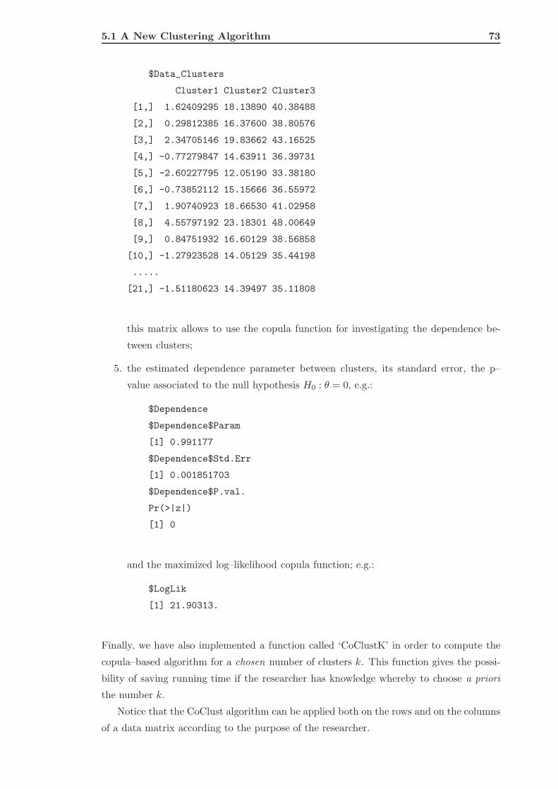
5.1 A New Clustering Algorithm 73
$Data_Clusters
Cluster1 Cluster2 Cluster3
[1,] 1.62409295 18.13890 40.38488
[2,] 0.29812385 16.37600 38.80576
[3,] 2.34705146 19.83662 43.16525
[4,] -0.77279847 14.63911 36.39731
[5,] -2.60227795 12.05190 33.38180
[6,] -0.73852112 15.15666 36.55972
[7,] 1.90740923 18.66530 41.02958
[8,] 4.55797192 23.18301 48.00649
[9,] 0.84751932 16.60129 38.56858
[10,] -1.27923528 14.05129 35.44198
.....
[21,] -1.51180623 14.39497 35.11808
this matrix allows to use the copula function for investigating the dependence be-
tween clusters;
5. the estimated dependence parameter between clusters, its standard error, the p–
value associated to the null hypothesis H0 : θ = 0, e.g.:
$Dependence
$Dependence$Param
[1] 0.991177
$Dependence$Std.Err
[1] 0.001851703
$Dependence$P.val.
Pr(>|z|)
[1] 0
and the maximized log–likelihood copula function; e.g.:
$LogLik
[1] 21.90313.
Finally, we have also implemented a function called ‘CoClustK’ in order to compute the
copula–based algorithm for a chosen number of clusters k. This function gives the possi-
bility of saving running time if the researcher has knowledge whereby to choose a priori
the number k.
Notice that the CoClust algorithm can be applied both on the rows and on the columns
of a data matrix according to the purpose of the researcher.
74 A copula–based clustering algorithm
5.2 Testing the New Algorithm
We test the CoClust algorithm by using two different copula functions (the Gaussian
and the Frank copula) and gaussian margins. We check the performance of the CoClust
algorithm for different situations and dependence settings.
5.2.1 CoClust of Gaussian Simulated Data
We perform a simulation study to test the CoClust algorithm by using a Gaussian copula.
The methodology is the same of Chapter 4, p. 45. We check the performance of the
CoClust by varying the number of clusters (or margins), type of margins, the value of
the dependence parameter and the sample size (number of rows and number of columns).
In particular, we perform simulations with 2, 3, 4 and 5 clusters, with well–separated,
overlapping and nested marginal distribution probability functions (see Chapter 4, Section
4.1.2, p. 46), with high and medium values of the dependence parameter (θ = 0.4 and
θ = 0.9). Finally, we apply the CoClust algorithm to the columns of the microarray data
matrix setting the argument nmaxmarg to 5.
For each number of clusters, we express the results in two tables; the first table,
summarizes the clustering procedure by representing:
- the percentage of replications with the correct number of identified clusters (p.n.c.
in brief);
- the percentage of replications with well–identified cluster sizes (p.w.s., (as defined in
Chapter 4, Section 4.1.3, p. 48));
and the analysis of the dependence by presenting:
- the mean value of the estimated dependence parameters post clustering over repli-
cations, θ∗;
- the cluster effect defined in Chapter 4, Section 4.1.3, p. 48;
- the percentage of acceptances (not rejection) about the null hypothesis on θ (ac-
cording to the dependence parameter value of the data generating process) over
replications with correct cluster sizes for all clusters, n.r.p. in brief.
The second kind of tables contains information about the goodness of fit clusters to mar-
gins. Its structure is equal to the tables shown in Chapter 4, Sections 4.2 (p. 51) and
4.3 (p. 58), with the only one difference that the percentages are about the ‘acceptances’
(and not about the ‘rejection’) of the null hypothesis on the mean, the variance and the
normality distribution.
We perform 200 replications for each setting.
In the case of data generated from a two–dimensional copula (tables 5.1 and 5.2, with
the number of observations for each margin equal to 1200, the number of rows equal to

5.2 Testing the New Algorithm 75
Table 5.1: CoClust performance: Gaussian copula, two clusters
Dependence Kind of Clustering Dependence
Parameter Margins p.n.c. p.w.s. θ∗ c.e. n.r.p.
Well–separated 100% 100% 0.8995 0.0005 94%
θ = 0.9 Overlapping 100% 100% 0.8999 0.0001 94%
Nested 100% 100% 0.8995 0.0005 94%
Well–separated 100% 100% −0.8840 1.2840 94%
θ = 0.4 Overlapping 100% 100% −0.8526 1.2526 94%
Nested 100% 100% 0.3975 0.0025 93.9%
400 and the number of columns equal to 6) the CoClust appears to work perfectly both
for the identification of the number of clusters and for the identification of the cluster
sizes (p.n.c. and p.w.s. are equal to 100%). The not rejection percentage of the null
hypothesis on the dependence parameter lies around 94% in each investigated case. As
for the goodness of fit, the CoClust works always perfectly except for the null hypothesis
on the mean value of the two clusters with low dependence (see Tab. 5.2 for θ = 0.4).
This ‘anomaly’ is coherent with the value of the cluster effect of the correspondent cases
even if we deem that also in these two cases the performance is acceptable in light of the
n.r.p. about the null hypothesis on θ and about other statistical tests (on variance and
Table 5.2: CoClust performance: Gaussian copula, two clusters
Dependence Kind of Mean Variance Normality
Parameter Margins C1 C2 C1 C2 C1 C2
Well–separated 95.5% 94% 100% 100% 100% 100%
θ = 0.9 Overlapping 95.5% 94.5% 100% 100% 100% 100%
Nested 93.5% 93% 100% 100% 100% 100%
Well–separated 0% 0% 100% 100% 100% 100%
θ = 0.4 Overlapping 0% 0% 100% 100% 100% 100%
Nested 96.5% 96.5% 100% 100% 100% 100%
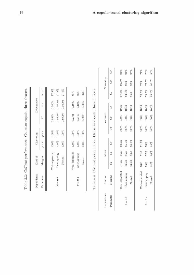
76 A copula–based clustering algorithm
Tab
le5.
3:C
oClu
stper
form
ance
:G
auss
ian
copula
,th
ree
clust
ers
Dep
enden
ceK
ind
of
Clu
ster
ing
Dep
enden
ce
Para
met
erM
arg
ins
p.n
.c.
p.w
.s.
θ∗
c.e
.n.r
.p.
Wel
l–se
para
ted
100%
100%
0.8
995
0.0
005
77.5
%
θ=
0.9
Over
lappin
g100%
100%
0.8
9997
0.0
0003
77.5
%
Nes
ted
100%
100%
0.8
9997
0.0
0003
77.5
%
Wel
l–se
para
ted
100%
100%
0.2
301
0.1
699
88%
θ=
0.4
Over
lappin
g100%
100%
0.2
710
0.1
290
88%
Nes
ted
100%
100%
0.3
988
0.0
012
88%
Tab
le5.
4:C
oClu
stper
form
ance
:G
auss
ian
copula
,th
ree
clust
ers
Dep
enden
ceK
ind
of
Mea
nVari
ance
Norm
ality
Para
met
erM
arg
ins
C1
C2
C3
C1
C2
C3
C1
C2
C3
Wel
l–se
para
ted
97.5
%95%
93.5
%100%
100%
100%
97.5
%95.5
%94%
θ=
0.9
Over
lappin
g96.5
%95%
95.5
%100%
100%
100%
94.5
%92%
94%
Nes
ted
96.5
%96%
96.5
%100%
100%
100%
95%
97%
95%
Wel
l-se
para
ted
70%
71%
71.5
%100%
100%
100%
70.5
%72%
71%
θ=
0.4
Over
lappin
g79%
77%
74%
100%
100%
100%
75.5
%77.5
%76%
Nes
ted
94%
96%
95%
100%
100%
100%
93.5
%97.5
%96%

5.2 Testing the New Algorithm 77
Tab
le5.
5:C
oClu
stper
form
ance
:G
auss
ian
copula
,fo
ur
clust
ers
Dep
enden
ceK
ind
of
Clu
ster
ing
Dep
enden
ce
Para
met
erM
arg
ins
p.n
.c.
p.w
.s.
θ∗
c.e
.n.r
.p.
Wel
l–se
para
ted
100%
100%
0.8
999
0.0
001
80.5
%
θ=
0.9
Over
lappin
g100%
100%
0.8
996
0.0
004
80.5
%
Nes
ted
100%
100%
0.8
999
0.0
001
80.5
%
Wel
l–se
para
ted
100%
100%
−0.3
065
0.7
065
80.5
%
θ=
0.4
Over
lappin
g100%
100%
−0.3
052
0.7
052
80.5
%
Nes
ted
100%
100%
0.3
9998
0.0
0002
80.5
%
Tab
le5.
6:C
oClu
stper
form
ance
:G
auss
ian
copula
,fo
ur
clust
ers
Dep
enden
ceK
ind
of
Mea
nVari
ance
Norm
ality
Para
met
erM
arg
ins
C1
C2
C3
C4
C1
C2
C3
C4
C1
C2
C3
C4
Wel
l–se
para
ted
92.5
%93.5
%90.5
%93%
100%
100%
100%
100%
93.5
%95.5
%94.5
%95%
θ=
0.9
Over
lappin
g95.5
%97.5
%96.5
%95.5
%100%
100%
100%
100%
96.5
%93%
95.5
%96.5
%
Nes
ted
95.5
%97.5
%94.5
%96.5
%100%
100%
100%
100%
91%
92.5
%97%
91.5
%
Wel
l–se
para
ted
0%
0%
0%
0%
100%
100%
100%
100%
0%
0%
0%
0%
θ=
0.4
Over
lappin
g0%
0%
0%
0%
100%
100%
100%
100%
0%
0%
0%
0%
Nes
ted
91.5
%93.5
%93%
93%
100%
100%
100%
100%
97.5
%95.5
%96.5
%96%
78 A copula–based clustering algorithm
normality distribution). In general, the performance appears to be independent of the
kind of margins and the level of dependence.
For the three clusters case, the number of observations for each margin is 800, the
number of rows is is 400 and the number of columns is 6. In this case (tables 5.3 and 5.4),
the CoClust works quite perfectly irrespective of the strength of dependence and the kind
of margins. The percentage of replications with correct number of identified clusters and
the percentage of replications with well–identified cluster sizes are full. The n.r.p. of H0
on the dependence parameter is greater in the case of θ = 0.4 (88%) than in the case of
θ = 0.9 (≈ 77%) but, in general, it is high to deem as very good the performance of the
algorithm. As for the goodness of fit, the not rejection percentages for the three computed
statistical tests are quite high. Hence, the CoClust algorithm seems capable to overcome
the limits of the K–means and hierarchical clustering outlined in the Chapter 4.
The performance of the CoClust on dependent data simulated via four–dimensional
copulas (tables 5.5 and 5.6 in which the number of observations for each margin is equal
to 800, the number of rows is equal to 400 and the number of columns is equal to 8) is
very similar to that of the two–clusters case. The analysis of clustering and the n.r.p.
about H0 on the dependence parameter are very satisfactory whereas the goodness of fit
clusters to margins as for the test on the mean values of the identified clusters and the
cluster effect show a possible weakness (see tables 5.5 and 5.6 for θ = 0.4). However, the
most important measures of performance are the p.n.c., the p.w.s. and the n.r.p. of the
null hypothesis on θ that make the performance acceptable. Even now, the performance
of the CoClust appears to be independent of the degree of overlap of margins and the level
of the dependence between observations.
Finally, as for the case of data drawn from a five–dimensional copula function (tables
5.7 and 5.8, with the number of observations for each margin equal to 100, the number of
rows equal to 50 and the number of columns equal to 10) the performance of the CoClust
is perfect as regards the analysis of the cluster performance (p.n.c. and p.w.s. are equal
to 100% in all settings investigated) and very good as regards the not rejection percentage
of H0 on the dependence parameter (n.r.p. is ≈ 77% in all cases) and the goodness
of fit (the percentage of not rejection for all computed statistical tests is > 85%). The
goodness of the CoClust is homogenous with respect to the kind of margins and the level
of dependence.
From this first set of simulations we may conclude that the CoClust algorithm is able
to
1. find always the correct number of clusters
2. find always the true number of observations in each identified clusters
3. overcome the limits of the other clustering methods (see Chapter 4, p. 45), working
perfectly in the case of nested margins and for high level of dependence
4. find the correct probability model for the margins

5.2 Testing the New Algorithm 79
Tab
le5.
7:C
oClu
stper
form
ance
:G
auss
ian
copula
,five
clust
ers
Dep
enden
ceK
ind
of
Clu
ster
ing
Dep
enden
ce
Para
met
erM
arg
ins
p.n
.c.
p.w
.s.
θ∗
c.e
.n.r
.p.
Wel
l–se
para
ted
100%
100%
0.8
985
0.0
015
77%
θ=
0.9
Over
lappin
g100%
100%
0.8
981
0.0
019
77%
Nes
ted
100%
100%
0.8
978
0.0
022
77%
Wel
l–se
para
ted
100%
100%
0.3
686
0.0
314
76.5
%
θ=
0.4
Over
lappin
g100%
100%
0.3
779
0.0
221
77%
Nes
ted
100%
100%
0.4
006
−0.0
006
77.3
%
Tab
le5.
8:C
oClu
stper
form
ance
:G
auss
ian
copula
,five
clust
ers
Dep
enden
ceK
ind
of
Mea
nVari
ance
Norm
ality
Para
met
erM
arg
ins
C1
C2
C3
C4
C5
C1
C2
C3
C4
C5
C1
C2
C3
C4
C5
Wel
l–se
para
ted
96.5
%94%
96.5
%95.5
%97.5
%100%
100%
100%
100%
100%
95%
94.5
%94.5
%95.5
%95%
θ=
0.9
Over
lappin
g96.5
%97.5
%97.5
%98.5
%96%
100%
100%
100%
100%
100%
96.5
%95.5
%96%
95.5
%93%
Nes
ted
95.5
%96.5
%98%
97.5
%97%
100%
100%
100%
100%
100%
93.5
%95.5
%95%
96%
95.5
%
Wel
l–se
para
ted
88.3
%87.2
%85.2
%89.8
%88.8
%100%
100%
100%
100%
100%
88.8
%89.8
%89.8
%87.2
%87.2
%
θ=
0.4
Over
lappin
g90.1
%92.2
%90.6
%91.2
%92.2
%100%
100%
100%
100%
100%
89.6
%89%
91.7
%90.6
%87.5
%
Nes
ted
98.4
%91%
93.7
%95.2
%94.2
%100%
100%
100%
100%
100%
97.9
%95.8
%94.7
%92%
96.3
%

80 A copula–based clustering algorithm
5. find the correct estimated value for the dependence parameter of the copula function.
We may conclude that the CoClust appears to be a satisfactory procedure to identify clus-
ters of dependent data irrespective of the strength of the dependence between observations
and the degree of overlap of marginal distribution functions. Moreover, we stress that the
CoClust algorithm allows to identify correctly the number of clusters.
5.2.2 CoClust of Frank Simulated Data
In this section we have replicated the simulations presented above by using a Frank copula.
As in the previous section, we made varying the number of clusters (or margins), the
type of margin, the value of the dependence parameter and the sample size. As for the
dependence parameter, we choose two values: 21 and 10, that indicate, respectively, high
and moderate dependence relationship between margins (similarly to 0.9 and 0.4 in the
Gaussian case). The number of rows, columns and observations for each margin are equal
to those used in the previous section.
Table 5.9: CoClust performance: Frank copula, two clusters
Dependence Kind of Clustering Dependence
Parameter Margins p.n.c. p.w.s. θ∗ c.e. n.r.p.
Well–separated 100% 100% 20.9548 0.0452 100%
θ = 21 Overlapping 100% 100% 20.9310 0.0690 100%
Nested 100% 100% 20.9979 0.0021 100%
Well–separated 100% 100% −11.1551 21.1551 100%
θ = 10 Overlapping 100% 100% 3.4029 6.5971 100%
Nested 100% 100% 9.9963 0.0037 100%
In the case of two clusters drawn from a Frank copula (tables 5.9 and 5.10) the CoClust
works perfectly both for the analysis of the obtained clustering with the p.n.c. and the
p.w.s. equals to 100% in each investigated case and for the analysis of dependence with
a not rejection percentage of H0 on the dependence parameter equal to 100% in each
analyzed case. These results indicate that the performance of the CoClust is independent
of the degree of overlap of margins and the strength of the dependence relationship between
observations. As regards the goodness of fit the CoClust works almost perfectly in the case
of high dependence between clusters. In the case of low dependence, instead, it appears to
work better in the nested margins case than in the non nested margins case according to
the correspondent cluster effect. In general, the performance of the CoClust is satisfactory.

5.2 Testing the New Algorithm 81
Table 5.10: CoClust performance: Frank copula, two clusters
Dependence Kind of Mean Variance Normality
Parameter Margins C1 C2 C1 C2 C1 C2
Well–separated 94% 95.5% 100% 100% 94% 96.5%
θ = 21 Overlapping 93% 93% 100% 100% 97% 96.5%
Nested 97.5% 95.5% 100% 100% 94.5% 94%
Well–separated 0.5% 0.5% 100% 100% 0.5% 0.5%
θ = 10 Overlapping 63% 64% 100% 100% 63% 62%
Nested 95% 93% 100% 100% 94% 94.5%
In the case of three clusters drawn from a Frank copula function (tables 5.11 and
5.12), the CoClust appears to work well showing a full percentage of replications in which
the number of identified clusters is correct, a full percentage of well–identified cluster
sizes and a quite full n.r.p. of the null hypothesis on the dependence parameter θ. Its
performance is equal in each situation investigated. As for the goodness of fit, the not
rejection percentages for any test is very high and close to 100% in nearly every situation
and dependence settings analyzed. The performance of the CoClust algorithm appears
to be independent of the degree of overlap of margins and of the dependence parameter
value.
The performance of the proposed algorithm in the case of four clusters (tables 5.13 and
5.14) is very similar to the previous case. In general, the CoClust appears able to correctly
identify the number of clusters and the cluster sizes in all replications (p.n.c. and p.w.s.
are equal to 100% in each situation investigated) and the true level of dependence in the
≈ 90% of replications. As for the goodness of fit margins to clusters, the performance is
satisfactory since the not rejection percentages of the null hypothesis on mean, variance
and normality distribution are equal to 100% in the majority of the situations investigated.
In the case of five clusters (see tables 5.15 and 5.16) the performance of the CoClust
is in general satisfactory. The percentage of replications with correct number of identified
clusters and with well–identified cluster sizes are full and the n.r.p. of the null hypothesis
on the dependence parameter θ are around 80%. The only case in which the obtained
results are not completely good is the case of well–separated margins and θ = 21 (n.r.p.
is ≈ 70%). As for the goodness of fit, the percentage of rejection about the computed
statistical tests are greater than 80% and most of them are at 100%.
In conclusion, the CoClust with the Frank copula model appears able to find always
the true number of clusters, the true cluster sizes and quite always the true dependence
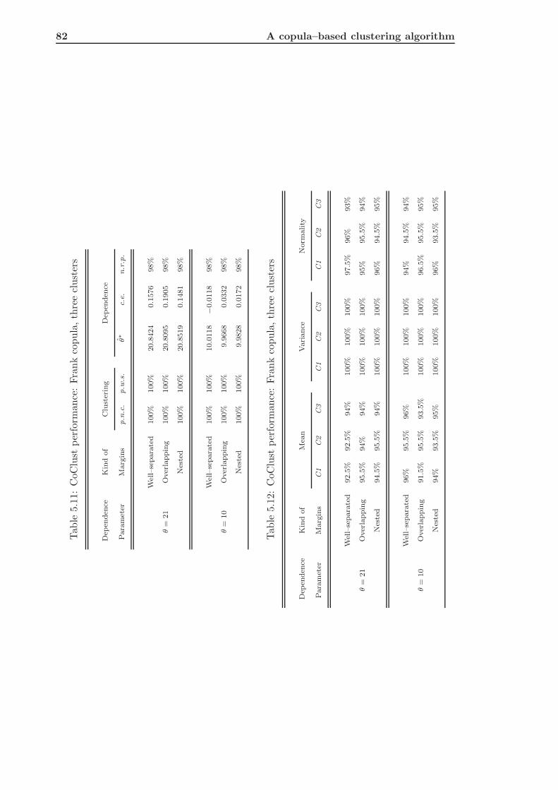
82 A copula–based clustering algorithm
Tab
le5.
11:
CoC
lust
per
form
ance
:Fra
nk
copula
,th
ree
clust
ers
Dep
enden
ceK
ind
of
Clu
ster
ing
Dep
enden
ce
Para
met
erM
arg
ins
p.n
.c.
p.w
.s.
θ∗
c.e
.n.r
.p.
Wel
l–se
para
ted
100%
100%
20.8
424
0.1
576
98%
θ=
21
Over
lappin
g100%
100%
20.8
095
0.1
905
98%
Nes
ted
100%
100%
20.8
519
0.1
481
98%
Wel
l–se
para
ted
100%
100%
10.0
118
−0.0
118
98%
θ=
10
Over
lappin
g100%
100%
9.9
668
0.0
332
98%
Nes
ted
100%
100%
9.9
828
0.0
172
98%
Tab
le5.
12:
CoC
lust
per
form
ance
:Fra
nk
copula
,th
ree
clust
ers
Dep
enden
ceK
ind
of
Mea
nVari
ance
Norm
ality
Para
met
erM
arg
ins
C1
C2
C3
C1
C2
C3
C1
C2
C3
Wel
l–se
para
ted
92.5
%92.5
%94%
100%
100%
100%
97.5
%96%
93%
θ=
21
Over
lappin
g95.5
%94%
94%
100%
100%
100%
95%
95.5
%94%
Nes
ted
94.5
%95.5
%94%
100%
100%
100%
96%
94.5
%95%
Wel
l–se
para
ted
96%
95.5
%96%
100%
100%
100%
94%
94.5
%94%
θ=
10
Over
lappin
g91.5
%95.5
%93.5
%100%
100%
100%
96.5
%95.5
%95%
Nes
ted
94%
93.5
%95%
100%
100%
100%
96%
93.5
%95%

5.2 Testing the New Algorithm 83
Tab
le5.
13:
CoC
lust
per
form
ance
:Fra
nk
copula
,fo
ur
clust
ers
Dep
enden
ceK
ind
of
Clu
ster
ing
Dep
enden
ce
Para
met
erM
arg
ins
p.n
.c.
p.w
.s.
θ∗
c.e
.n.r
.p.
Wel
l–se
para
ted
100%
100%
20.7
585
0.2
415
83.3
%
θ=
21
Over
lappin
g100%
100%
20.9
215
0.0
785
90.9
%
Nes
ted
100%
100%
20.4
744
0.5
256
90.9
%
Wel
l–se
para
ted
100%
100%
10.0
101
−0.0
101
90.9
%
θ=
10
Over
lappin
g100%
100%
10.0
025
−0.0
025
90.9
%
Nes
ted
100%
100%
10.1
120
−0.1
120
90.9
%
Tab
le5.
14:
CoC
lust
per
form
ance
:Fra
nk
copula
,fo
ur
clust
ers
Dep
enden
ceK
ind
of
Mea
nVari
ance
Norm
ality
Para
met
erM
arg
ins
C1
C2
C3
C4
C1
C2
C3
C4
C1
C2
C3
C4
Wel
l–se
para
ted
91.7
%91.7
%91.7
%91.7
%91.7
%91.7
%91.7
%91.7
%83.3
%83.3
%83.3
%91.7
%
θ=
21
Over
lappin
g100%
100%
91%
91%
100%
100%
100%
100%
100%
100%
90.9
%90.9
%
Nes
ted
81.8
%81.8
%72.7
%81.8
%100%
100%
100%
100%
90.9
%100%
100%
100%
Wel
l–se
para
ted
100%
100%
100%
100%
100%
100%
100%
100%
100%
100%
90.9
%90.9
%
θ=
10
Over
lappin
g100%
100%
90.9
%100%
100%
100%
100%
100%
100%
100%
100%
90.9
%
Nes
ted
100%
100%
100%
90.9
%100%
100%
100%
100%
100%
100%
90.9
%90.9
%

84 A copula–based clustering algorithm
Tab
le5.
15:
CoC
lust
per
form
ance
:Fra
nk
copula
,five
clust
ers
Dep
enden
ceK
ind
of
Clu
ster
ing
Dep
enden
ce
Para
met
erM
arg
ins
p.n
.c.
p.w
.s.
θ∗
c.e
.n.r
.p.
Wel
l–se
para
ted
100%
100%
19.9
850
1.0
150
66.7
%
θ=
21
Over
lappin
g100%
100%
20.6
655
0.3
345
80%
Nes
ted
100%
100%
20.9
558
0.0
442
80%
Wel
l–se
para
ted
100%
100%
9.6
829
0.3
171
80%
θ=
10
Over
lappin
g100%
100%
9.5
075
0.4
925
80%
Nes
ted
100%
100%
10.4
438
−0.4
438
80%
Tab
le5.
16:
CoC
lust
per
form
ance
:Fra
nk
copula
,five
clust
ers
Dep
enden
ceK
ind
of
Mea
nVari
ance
Norm
ality
Para
met
erM
arg
ins
C1
C2
C3
C4
C5
C1
C2
C3
C4
C5
C1
C2
C3
C4
C5
Wel
l–se
para
ted
83.3
%83.3
%83.3
%83.3
%83.3
%83.3
%83.3
%83.3
%83.3
%83.3
%83.3
%83.3
%83.3
%83.3
%83.3
%
θ=
21
Over
lappin
g100%
100%
100%
100%
100%
100%
100%
100%
100%
100%
100%
80%
100%
80%
100%
Nes
ted
100%
100%
100%
100%
100%
100%
100%
100%
100%
100%
100%
100%
80%
100%
100%
Wel
l–se
para
ted
80%
100%
100%
80%
100%
100%
100%
100%
100%
100%
100%
100%
100%
100%
80%
θ=
10
Over
lappin
g100%
100%
100%
100%
100%
100%
100%
100%
100%
100%
100%
100%
100%
100%
100%
Nes
ted
100%
100%
100%
100%
100%
100%
100%
100%
100%
100%
80%
80%
100%
100%
80%

5.3 Comparison between CoClust and mClust 85
relationship irrespectively of the kind of margins, the number of clusters and the strength of
the dependence relationship. As in the Gaussian cases, the algorithm allows us to overcome
the limits of the two clustering methods investigated in Chapter 4 and to identify clusters
of dependent data respecting the true underlying dependence structure.
5.2.3 Conclusions about Simulation Results
From these simulations we may argue that the main advantages of this new clustering
algorithm are the following:
1. it is able to find clusters of observations (gene expressions or experimental condi-
tions) according to the dispersion structure of the data allowing to uncover the true
dependence relationship in gene expressions data
- irrespective of the degree of overlap of margins;
- irrespective of the level of dependence between margins;
2. it is not necessary to know a priori the number of clusters;
3. it does not require to have a starting classification;
4. it allows to find the k–plets of observations that are dependent;
5. it can account for complex dependence relationship between gene expressions;
6. it overcomes the limits of the K–means and hierarchical clustering (see Chapter 4).
In the next section we are going to compare the CoClust with an other class of clus-
tering techniques based on statistical models: the model–based clustering (Fraley and
Raftery, 1998, 1999, 2000 and 2007).
5.3 Comparison between CoClust and mClust
In this section we perform a simulation study in order to compare the CoClust with the
model–based clustering algorithm (Chapter 1, Section 1.2.3, p. 13) in the same situations
and dependence settings outlined in the previous sections.
5.3.1 mClust of Gaussian Simulated Data
The design of the simulation study is the same as that of the previous sections. We have
set the minimum number of mixture components (clusters) to 2 and the maximum number
to 5. The model–based algorithm is applied to the data put in one column in order to
communicate to the EM algorithm that the data in each cluster are one–dimensional.
All other factors vary as in the simulation study performed in the previous sections and
the obtained results are shown in two tables whose structure is like those of the previous
sections.

86 A copula–based clustering algorithm
Since the ‘mClust’ is not always able to identify the correct number of clusters, the
statistical test on the mean, the variance and the normality for each cluster are computed
on the number of replications with well–identified number of clusters. Finally, notice that
when in the tables concerning the test on the clusters you find ‘NA’ (‘not available’), it
means that it has not been possible to compute the value since there were no correct
results for any replication.
Table 5.17: mClust performance: Gaussian copula, two clusters
Dependence Kind of Clustering Dependence
Parameter Margins p.n.c. p.w.s. θ∗ c.e. n.r.p.
Well–separated 100% 34% 0.3848 0.5152 18.5%
θ = 0.9 Overlapping 100% 13% 0.0805 0.8195 0.5%
Nested 81.5% 0% −0.0097 0.9097 0%
Well–separated 100% 37% 0.1552 0.2448 27%
θ = 0.4 Overlapping 100% 11% 0.0421 0.3579 0.5%
Nested 84% 0% 0.0077 0.3923 4.5%
Table 5.18: mClust performance: Gaussian copula, two clusters
Dependence Kind of Mean Variance Normality
Parameter Margins C1 C2 C1 C2 C1 C2
Well–separated 94.5% 93.5% 100% 100% 96% 95%
θ = 0.9 Overlapping 93.5% 92.5% 100% 100% 92.5% 93%
Nested 31.9% 22.1% 93.3% 93.3% 30% 11.7%
Well–separated 97.5% 93.5% 100% 100% 94% 92.5%
θ = 0.4 Overlapping 97% 91% 100% 100% 95% 95.5%
Nested 22% 23.2% 92.9% 92.9% 26.8% 11.3%
In the two clusters case (tables 5.17 and 5.18) note that the model–based clustering
is always able to identify the correct number of clusters in the not nested margins case
and almost always in the nested margins case. As for the p.w.s., instead, the mClust
fails in each situation and dependence settings investigated. This failure influences the

5.3 Comparison between CoClust and mClust 87
failure in finding the true underlying dependence relationship between clusters. However,
as for the n.r.p. of the null hypothesis on the dependence parameter the performance
of the mClust appears to get worse as long as the margins become overlapping. This
result is confirmed by the trend of the cluster effect and the value of the mean of θ over
replications. As for the goodness of fit, the mClust appears to be a good technique to
identify the correct probability model even if the most important measures of performance
reveal the incapability of the mClust in finding the true dependence relationship between
clusters.
In Tab. 5.19 we note that the performance of the mClust is perfect as for the percentage
of replications with correct number of identified clusters in the not nested margins case
but it fails in the nested margins one decreasing dramatically from 100% to 17%. The
performance worsen as the level of overlap increases (see the trend of the c.e and the n.r.p.
of H0 on θ). As for the goodness of fit (Tab. 5.20), the mClust appears to be quite able in
finding the correct probability model for margins even if, also here, its performance gets
worse with the degree of overlap, similarly to the behavior of the K–means and hierarchical
clustering methods (Chapter 4, Sections 4.2, p. 51 and 4.3, p. 58).
Also in the case of four clusters (Tab. 5.21) the performance of the model–based
clustering appears to be dependent on the degree of overlap of margins as for the p.n.c.
that decreases from 100% in the case of well–separated margins to 0% in the case of
nested margins. The cluster effect, the mean of θ over replications and the n.r.p. of the
null hypothesis on the dependence parameter reveal the failure of the mClust in finding the
true dependence relationship between clusters. As for the goodness of fit (Tab. 5.22) the
mClust clustering techniques appears able to identify the true mean and variance values
and the normality distribution (in almost two of the four clusters) for the majority of the
replications in the cases of not nested margins. Notice that we do not have replications in
which is possible to compute the statistical tests in the case of nested margins. In general,
the performance of the mClust in grouping dependent data is not satisfactory.
In the case of five clusters (tables 5.23 and 5.24) the mClust works well as for the
percentage of replications with correct number of identified clusters in not nested margins
(p.n.c. are ≈ 80%) case but totally fails in the nested margins case. As for the other
measures of performance shown in Tab. 5.23, the mClust fails in each investigated case
even if as for the goodness of clusters for the not nested margins cases (Tab. 5.24) appears
to be quite good.
We may conclude that the model–based clustering is able to identify the correct number
of clusters in the not nested margins case irrespective of the kind of dependence relationship
between themselves but it appears not able to group dependent observations not being
able to identify the correct value of θ in each situation investigated. Moreover, the mClust
performance is not independent of the kind of margins and it does not allow to overcome
the limits of the K–means and hierarchical clustering analyzed in Chapter 4. It appears
not adequate to the purpose of clustering dependent (microarray) data. Comparing these

88 A copula–based clustering algorithm
Tab
le5.
19:
mC
lust
per
form
ance
:G
auss
ian
copula
,th
ree
clust
ers
Dep
enden
ceK
ind
of
Clu
ster
ing
Dep
enden
ce
Para
met
erM
arg
ins
p.n
.c.
p.w
.s.
θ∗
c.e
.n.r
.p.
Wel
l–se
para
ted
100%
34%
0.3
537
0.6
363
8%
θ=
0.9
Over
lappin
g100%
14%
0.2
176
0.6
824
1%
Nes
ted
17%
0%
−0.0
119
0.9
119
0%
Wel
l–se
para
ted
100%
29.5
%0.1
663
0.2
337
14%
θ=
0.4
Over
lappin
g100%
15.5
%0.0
798
0.3
202
1%
Nes
ted
22%
0%
−0.0
155
0.4
155
0%
Tab
le5.
20:
mC
lust
per
form
ance
:G
auss
ian
copula
,th
ree
clust
ers
Dep
enden
ceK
ind
of
Mea
nVari
ance
Norm
ality
Para
met
erM
arg
ins
C1
C2
C3
C1
C2
C3
C1
C2
C3
Wel
l–se
para
ted
93.5
%92.5
%95%
100%
100%
100%
93.5
%94.5
%97%
θ=
0.9
Over
lappin
g94%
92%
91%
100%
100%
100%
95.5
%96%
96.5
%
Nes
ted
70.6
%26.5
%0%
100%
100%
100%
70.6
%29.4
%5.9
%
Wel
l–se
para
ted
94.5
%93.5
%92.5
%100%
100%
100%
95%
97.5
%95.5
%
θ=
0.4
Over
lappin
g92%
93.5
%93%
100%
100%
100%
96.5
%96.5
%96.5
%
Nes
ted
65.9
%18.2
%9.1
%100%
100%
100%
70.5
%20.5
%9.1
%

5.3 Comparison between CoClust and mClust 89
Tab
le5.
21:
mC
lust
per
form
ance
:G
auss
ian
copula
,fo
ur
clust
ers
Dep
enden
ceK
ind
of
Clu
ster
ing
Dep
enden
ce
Para
met
erM
arg
ins
p.n
.c.
p.w
.s.
θ∗
c.e
.n.r
.p.
Wel
l–se
para
ted
100%
1%
0.0
855
0.8
145
0%
θ=
0.9
Over
lappin
g100%
0.5
%0.0
418
0.8
582
0%
Nes
ted
0%
0%
NA
NA
NA
Wel
l–se
para
ted
100%
0.5
%0.0
330
0.3
670
0%
θ=
0.4
Over
lappin
g100%
0%
0.0
203
0.3
797
0%
Nes
ted
0%
0%
NA
NA
NA
Tab
le5.
22:
mC
lust
per
form
ance
:G
auss
ian
copula
,fo
ur
clust
ers
Dep
enden
ceK
ind
of
Mea
nVari
ance
Norm
ality
Para
met
erM
arg
ins
C1
C2
C3
C4
C1
C2
C3
C4
C1
C2
C3
C4
Wel
l–se
para
ted
96.5
%94%
27%
24%
100%
100%
100%
100%
95.5
%96.5
%21.5
%0%
θ=
0.9
Over
lappin
g94.5
%94%
27%
18.5
%100%
100%
100%
100%
94.5
%93.5
%21%
0.5
%
Nes
ted
NA
NA
NA
NA
NA
NA
NA
NA
NA
NA
NA
NA
Wel
l–se
para
ted
94.5
%94.5
%21.5
%18.5
%100%
100%
100%
100%
97.5
%97%
23%
1%
θ=
0.4
Over
lappin
g97%
98%
24.5
%31%
100%
100%
100%
100%
94.5
%91%
14.5
%1%
Nes
ted
NA
NA
NA
NA
NA
NA
NA
NA
NA
NA
NA
NA
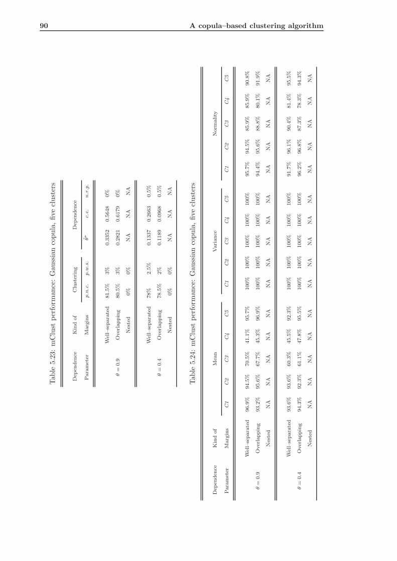
90 A copula–based clustering algorithm
Tab
le5.
23:
mC
lust
per
form
ance
:G
auss
ian
copula
,five
clust
ers
Dep
enden
ceK
ind
of
Clu
ster
ing
Dep
enden
ce
Para
met
erM
arg
ins
p.n
.c.
p.w
.s.
θ∗
c.e
.n.r
.p.
Wel
l–se
para
ted
81.5
%3%
0.3
352
0.5
648
0%
θ=
0.9
Over
lappin
g80.5
%3%
0.2
821
0.6
179
0%
Nes
ted
0%
0%
NA
NA
NA
Wel
l–se
para
ted
78%
2.5
%0.1
337
0.2
663
0.5
%
θ=
0.4
Over
lappin
g78.5
%2%
0.1
189
0.0
968
0.5
%
Nes
ted
0%
0%
NA
NA
NA
Tab
le5.
24:
mC
lust
per
form
ance
:G
auss
ian
copula
,five
clust
ers
Dep
enden
ceK
ind
of
Mea
nVari
ance
Norm
ality
Para
met
erM
arg
ins
C1
C2
C3
C4
C5
C1
C2
C3
C4
C5
C1
C2
C3
C4
C5
Wel
l–se
para
ted
96.9
%94.5
%70.5
%41.1
%95.7
%100%
100%
100%
100%
100%
95.7
%94.5
%85.9
%85.9
%90.8
%
θ=
0.9
Over
lappin
g93.2
%95.6
%67.7
%45.3
%96.9
%100%
100%
100%
100%
100%
94.4
%95.6
%88.8
%80.1
%91.9
%
Nes
ted
NA
NA
NA
NA
NA
NA
NA
NA
NA
NA
NA
NA
NA
NA
NA
Wel
l–se
para
ted
93.6
%93.6
%60.3
%45.5
%92.3
%100%
100%
100%
100%
100%
91.7
%96.1
%90.4
%81.4
%95.5
%
θ=
0.4
Over
lappin
g94.3
%92.3
%61.1
%47.8
%95.5
%100%
100%
100%
100%
100%
96.2
%96.8
%87.3
%78.3
%94.3
%
Nes
ted
NA
NA
NA
NA
NA
NA
NA
NA
NA
NA
NA
NA
NA
NA
NA

5.3 Comparison between CoClust and mClust 91
results with the performance of the CoClust algorithm, we may conclude that in general
the CoClust performs better than the mClust method. The only drawback of the CoClust
in its current implementation is that it is more computationally expensive than the mClust.
5.3.2 mClust of Frank Simulated Data
We analyze the performance of the model–based clustering on dependent data simulated
via a Frank copula. The setting is the same of that followed in previous analysis as well
as the two kind of tables in which the results are shown.
Table 5.25: mClust performance: Frank copula, two clusters
Dependence Kind of Clustering Dependence
Parameter Margins p.n.c. p.w.s. θ∗ c.e. n.r.p.
Well–separated 99.5% 32% 5.9041 15.0959 19.5%
θ = 21 Overlapping 100% 14% 0.8982 20.1018 0%
Nested 81.5% 0% −0.0549 21.0549 0%
Well–separated 100% 33% 3.3577 6.6423 21.5%
θ = 10 Overlapping 100% 13% 0.6432 9.3568 0.5%
Nested 83% 0% −0.0115 10.0115 0%
Table 5.26: mClust performance: Frank copula, two clusters
Dependence Kind of Mean Variance Normality
Parameter Margins C1 C2 C1 C2 C1 C2
Well–separated 96% 94.5% 100% 100% 97% 98.5%
θ = 21 Overlapping 93% 94% 100% 100% 97% 96%
Nested 25.8% 22.1% 91.4% 91.4% 28.8% 14.1%
Well–separated 95% 93% 100% 100% 98% 96%
θ = 10 Overlapping 92% 91.5% 100% 100% 95% 97%
Nested 30.7% 10.8% 92.2% 92.2% 31.3% 4.2%
The model–based clustering works very well for the identification of the number of

92 A copula–based clustering algorithm
Tab
le5.
27:
mC
lust
per
form
ance
:Fra
nk
copula
,th
ree
clust
ers
Dep
enden
ceK
ind
of
Clu
ster
ing
Dep
enden
ce
Para
met
erM
arg
ins
p.n
.c.
p.w
.s.
θ∗
c.e
.n.r
.p.
Wel
l–se
para
ted
100%
32.5
%4.7
565
16.2
435
9%
θ=
21
Over
lappin
g100%
16%
1.8
983
19.1
017
0.5
%
Nes
ted
18.5
%0%
−0.0
783
21.0
783
0%
Wel
l–se
para
ted
100%
25.5
%2.6
684
7.3
316
9.5
%
θ=
10
Over
lappin
g100%
16.5
%1.2
461
8.7
539
0%
Nes
ted
24.5
%0%
−0.0
111
10.0
111
0%
Tab
le5.
28:
mC
lust
per
form
ance
:Fra
nk
copula
,th
ree
clust
ers
Dep
enden
ceK
ind
of
Mea
nVari
ance
Norm
ality
Para
met
erM
arg
ins
C1
C2
C3
C1
C2
C3
C1
C2
C3
Wel
l–se
para
ted
92.5
%93%
94.5
%100%
100%
100%
95%
95.5
%93%
θ=
21
Over
lappin
g93%
91.5
%93%
100%
100%
100%
92.5
%97.5
%96%
Nes
ted
75.7
%16.2
%2.7
%100%
100%
100%
70.3
%16.2
%2.7
%
Wel
l–se
para
ted
94%
94%
95%
100%
100%
100%
96%
93.5
%98.5
%
θ=
10
Over
lappin
g95%
94.5
%94%
100%
100%
100%
98%
91%
96%
Nes
ted
55.1
%22.5
%12.3
%100%
100%
100%
55.1
%28.6
%12.3
%
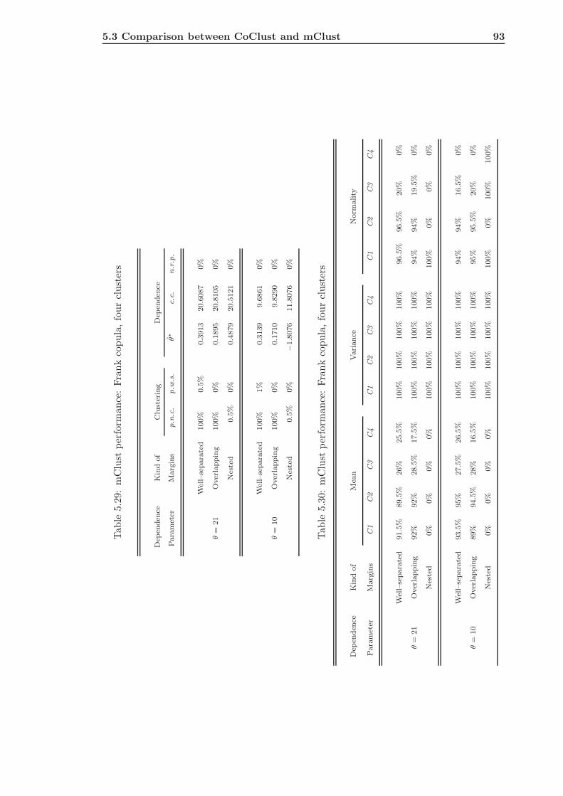
5.3 Comparison between CoClust and mClust 93
Tab
le5.
29:
mC
lust
per
form
ance
:Fra
nk
copula
,fo
ur
clust
ers
Dep
enden
ceK
ind
of
Clu
ster
ing
Dep
enden
ce
Para
met
erM
arg
ins
p.n
.c.
p.w
.s.
θ∗
c.e
.n.r
.p.
Wel
l–se
para
ted
100%
0.5
%0.3
913
20.6
087
0%
θ=
21
Over
lappin
g100%
0%
0.1
895
20.8
105
0%
Nes
ted
0.5
%0%
0.4
879
20.5
121
0%
Wel
l–se
para
ted
100%
1%
0.3
139
9.6
861
0%
θ=
10
Over
lappin
g100%
0%
0.1
710
9.8
290
0%
Nes
ted
0.5
%0%
−1.8
076
11.8
076
0%
Tab
le5.
30:
mC
lust
per
form
ance
:Fra
nk
copula
,fo
ur
clust
ers
Dep
enden
ceK
ind
of
Mea
nVari
ance
Norm
ality
Para
met
erM
arg
ins
C1
C2
C3
C4
C1
C2
C3
C4
C1
C2
C3
C4
Wel
l–se
para
ted
91.5
%89.5
%26%
25.5
%100%
100%
100%
100%
96.5
%96.5
%20%
0%
θ=
21
Over
lappin
g92%
92%
28.5
%17.5
%100%
100%
100%
100%
94%
94%
19.5
%0%
Nes
ted
0%
0%
0%
0%
100%
100%
100%
100%
100%
0%
0%
0%
Wel
l–se
para
ted
93.5
%95%
27.5
%26.5
%100%
100%
100%
100%
94%
94%
16.5
%0%
θ=
10
Over
lappin
g89%
94.5
%28%
16.5
%100%
100%
100%
100%
95%
95.5
%20%
0%
Nes
ted
0%
0%
0%
0%
100%
100%
100%
100%
100%
0%
100%
100%

94 A copula–based clustering algorithm
clusters irrespective of the kind of margins and the level of dependence (see Tab. 5.25)
whereas it does not have a satisfactory performance as for all other measures of perfor-
mance. In the case of nested margins, it totally fails as for the p.w.s., the c.e. and the
n.r.p. of H0 on the dependence parameter. Notice that as regards the percentage of
well–identified cluster sizes and the not rejection percentage of the null hypothesis on the
dependence parameter, the performance of the mClust gets worse as the margins become
more and more overlapping. This remark is valid also for the goodness of fit (see Tab.
5.26) even if for this kind of analysis the performance of the mClust improves with respect
to the analysis of dependence.
In the case of three clusters drawn from a Frank copula, the performance of the mClust
does not change. It gets worse as long as the margins become overlapping up to a total
failure in the nested margins cases. The only measure of performance that shows a good
performance in the not nested margins cases is the percentage of correct number of clusters
(see Tab. 5.27). As for the n.r.p. of H0 on the dependence parameter the mClust appears
to be better in the two cluster case but it is still unsatisfactory. The goodness of fit (Tab.
5.28) is very good in the not nested cases but the overall performance of the mClust appears
not adequate to group dependent data since it does not allow us to recover correctly the
underlying dependence structure.
Working with four clusters of dependent data, the mClust totally fails in the analysis
of dependence (see Tab. 5.29) with a zero percentage of not rejection of the null hypothesis
on θ in all the cases investigated. Also here, the mClust appears to be able to identify
the correct number of clusters in the not nested margins cases whereas it fails in the
identification of the cluster sizes. The c.e. is very high in each situations investigated,
irrespective of the level of dependence and the kind of margins. The goodness of fit (Tab.
5.30) is quite good in the not nested margins cases but it fails in the nested margins case.
Finally, the model–based clustering does not allow us to recover the true underlying
dependence structure in each dependence settings investigated, irrespective of the kind of
margins, also in the case of five clusters. Indeed, the not rejection percentage of H0 on the
dependence parameter is always equal to zero (Tab. 5.31) and the cluster effect is very
high in each investigated cases. The failure likely lies in that of the identification of the
cluster sizes: the p.w.s. is always close to zero. If we focus our attention only on the not
nested margins cases, the only satisfactory measure of performance is the percentage of
replications in which the number of identified clusters is correct. The goodness of fit (Tab.
5.32) is very good with exception of the nested margins case for which we do not have
replications in which the number of clusters has been correctly identified. In conclusion,
this set of simulations confirms the findings of the Gaussian case since the model–based
clustering does not appear to be appropriate to group dependent data because it does
not allow us to discover the true dependence structure of the data generating process.
Moreover, its performance appears to be dependent on the degree of overlap of margins
like the other two clustering techniques investigated in Chapter 4 but independent of the
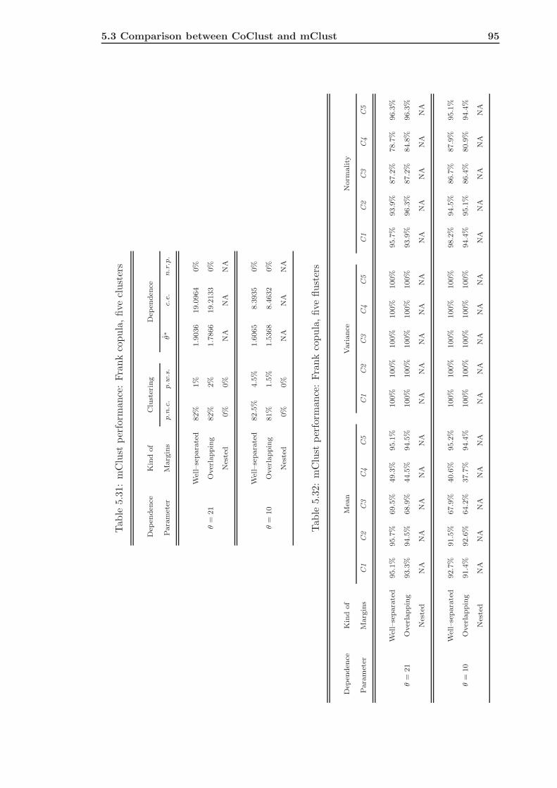
5.3 Comparison between CoClust and mClust 95
Tab
le5.
31:
mC
lust
per
form
ance
:Fra
nk
copula
,five
clust
ers
Dep
enden
ceK
ind
of
Clu
ster
ing
Dep
enden
ce
Para
met
erM
arg
ins
p.n
.c.
p.w
.s.
θ∗
c.e
.n.r
.p.
Wel
l–se
para
ted
82%
1%
1.9
036
19.0
964
0%
θ=
21
Over
lappin
g82%
2%
1.7
866
19.2
133
0%
Nes
ted
0%
0%
NA
NA
NA
Wel
l–se
para
ted
82.5
%4.5
%1.6
065
8.3
935
0%
θ=
10
Over
lappin
g81%
1.5
%1.5
368
8.4
632
0%
Nes
ted
0%
0%
NA
NA
NA
Tab
le5.
32:
mC
lust
per
form
ance
:Fra
nk
copula
,five
flust
ers
Dep
enden
ceK
ind
of
Mea
nVari
ance
Norm
ality
Para
met
erM
arg
ins
C1
C2
C3
C4
C5
C1
C2
C3
C4
C5
C1
C2
C3
C4
C5
Wel
l–se
para
ted
95.1
%95.7
%69.5
%49.3
%95.1
%100%
100%
100%
100%
100%
95.7
%93.9
%87.2
%78.7
%96.3
%
θ=
21
Over
lappin
g93.3
%94.5
%68.9
%44.5
%94.5
%100%
100%
100%
100%
100%
93.9
%96.3
%87.2
%84.8
%96.3
%
Nes
ted
NA
NA
NA
NA
NA
NA
NA
NA
NA
NA
NA
NA
NA
NA
NA
Wel
l–se
para
ted
92.7
%91.5
%67.9
%40.6
%95.2
%100%
100%
100%
100%
100%
98.2
%94.5
%86.7
%87.9
%95.1
%
θ=
10
Over
lappin
g91.4
%92.6
%64.2
%37.7
%94.4
%100%
100%
100%
100%
100%
94.4
%95.1
%86.4
%80.9
%94.4
%
Nes
ted
NA
NA
NA
NA
NA
NA
NA
NA
NA
NA
NA
NA
NA
NA
NA

96 A copula–based clustering algorithm
value of the dependence parameter.
5.4 Discussion
In this chapter, we have described a new clustering algorithm based on copula functions.
This algorithm has been tested on simulated data drawn from Gaussian and Frank copula
in different situations and dependence settings. We have found that the algorithm is able
to recover the true underlying dependence relationship between observations grouped in
different clusters irrespective of the kind of margins, the value of the dependence parameter
and the copula model.
Interestingly, the CoClust algorithm has other peculiar characteristics. In fact, it is
able to identify the correct number of clusters independently of the kind of dependence
relationship between clusters allowing to overcome this difficult matter. Moreover, it
does not require a starting classification of data because in the first two steps of the
algorithm it tests all possible combinations of k–plet of data choosing that maximizes the
log–likelihood copula function. This allows to choose the best number of clusters, that is,
the number of clusters and the k–plet that are better fitted by a copula function. In the
following steps, the algorithm tests all possible dispositions of the remaining observations
and selects the k–plet that preserves the dependence relationship and is the best fitted by
the copula. Taking in account the order in the k–plet of observations enables to choose
at what cluster to assign each observation. The order is very important to preserve the
dependence structure of the data. In the proposed algorithm there are not sources of
coming bias either from the a priori choice of the number of clusters or from a starting
classification.
A drawback of the CoClust is its computational complexity even if there is room for
further optimization under this aspect. Indeed, a new faster version is in progress. It is
based on a change in the last two steps of the procedure described in Section 5.1.1 that
allows to save CPU time. Once k is chosen, the algorithm does not explore anymore the
whole space of the all possible dispositions of each k–plet but at each iteration it selects
a subspace of all possible combinations of remaining k–plets on the basis of the result
obtained at the previous step and computes all possible dispositions just for a specific
k–plet candidate to allocation on the basis of the copula–based split up rule.
We have also compared the CoClust with another well–known clustering technique
based on probability models and we have found that the latter appears not able to model
the true dependence relationship between observations. Moreover it does not allow to
overcome the limits of the K–means and hierarchical clustering methods investigated in
the previous chapter working worse in the not nested margins cases than in the nested
margins ones. The algorithm proposed, instead, allows to achieve such tasks since its
performance is independent of the degree of overlap of margins.
In the next chapter we are going to apply the CoClust algorithm to a real microarray

5.4 Discussion 97
data set.


Chapter 6
Applying the CoClust to Real
Data
This chapter is dedicated to the application of the CoClust algorithm to a real microarray
data set. The attention focuses on the breast tumors data discussed in Hedenfalk et al.
(2001). The main purpose is to discover new information about the relationship between
genes observed in three different cancer samples. At the same time, we apply the CoClust
to the columns of the whole data matrix in order to verify whether the algorithm is able
to group correctly the types of mutation.
6.1 Introduction
In this section we describe the microarray data set we use for the applications of the
CoClust algorithm and the preliminary transformations and analysis performed.
6.1.1 Description of the Data Set
Hedenfalk et al. (2001) obtained RNA from samples of primary breast tumors in patients
who had a family history of breast or ovarian cancer, or both, that was compatible with
a dominant mode of inheritance were referred for genetic counseling to the Oncogenetic
Clinic of Lund University Hospital. Biopsy specimens of primary breast tumors from
patients with germ–line mutations of BRCA1 (seven patients) or BRCA2 (eight tumors
from seven patients) were selected for analysis. In addition, seven patients with sporadic
cases of primary breast cancer whose family history was unknown were also identified.
Summarizing, 21 patients were observed: seven carriers of the BRCA1 mutation, seven
carriers of the BRCA2 mutation and seven patients with sporadic cases of breast cancer.
They were compared with a microarray of 6512 complementary DNA clones of 5361 genes.
The data set is available at
http://research.nhgri.nih.gov/microarray/NEJM_Supplement/.
99

100 Applying the CoClust to Real Data
The (tab–delimited) text file contains the gene expression ratios from 21 microarray ex-
periments, the patients ID (first row), the mutation classification for each experiment:
BRCA1, BRCA2, Sporadic (second row) and the experiment ID (third row); the first
three columns contain information about the microtiter plate ID where each clone is phys-
ically locates, the IMAGE clone ID and the Clone Title, respectively as follows:
NEJM-PatientID 1 5 3..
Mutation BRCA1 BRCA1 BRCA1..
PlatePosition ImageCloneID Title s1996 s1822 s1714..
HK1A1 21652 "catenin" 0.15 0.22 0.3..
HK1A2 22012 "ADP-ribosylation fac.3" 1.54 1.27 0.76..
...
Hedenfalk et al. (2001) select genes based on the following criteria:
- average fluorescent intensity (level expression) of more than 2.500 (gray level) across
all 21 samples;
- average spot area of more than 40 pixels across all 21 samples;
- no more than one sample in which the spot area is zero pixel.
They obtain 3226 genes. Gene expression ratios included in the data file were derived
from the ratio of fluorescent intensity (proportional to the gene expression level) from a
tumor sample and fluorescent intensity from a common reference sample (MCF–10A). The
common reference sample is used for all 21 microarray experiments. Therefore, the ratio
may take value from 0 to infinity.
6.1.2 Preliminary Analysis
First of all, we perform a logarithmic–transform to convert the ratio of the 3226 genes in
order to achieve the symmetric property from over–expression to under–expression range.
Second, we focus our attention on the list of 51 genes whose variation in expression
among all experiments best differentiated among these types of cancers (Hedenfalk et al.,
2001). Consequently, we divide the database in three different sets of gene expressions
according to the type of mutation observed: BRCA1, BRCA2 and Sporadic. We are
going to apply the CoClust algorithm to such three sets of gene expressions in order to
investigate the changes in the kind and the strength of the dependence between genes
according to the type of tumor sample (mutation).
Third, we focus our attention on the whole data set in order to apply the CoClust
algorithm to its columns (kind of mutation). The purpose is to test the capability of the
CoClust of finding groups according to the kind of mutation.
In the analysis we omit the column number 10 that contains the genes of a BRCA2
cancer sample of the same patient whose genes were put into column 7.

6.2 Application of the CoClust to Hedenfalk Data 101
6.2 Application of the CoClust to Hedenfalk Data
In this section we describe the analysis performed on the Hedenfalk et al. (2001) data
set. The first part is dedicated to the application of the CoClust algorithm to the gene
expressions recorded for three different tumor samples. In the second part the CoClust
will be applied to the whole data set in order to test its capability in distinguishing the
three samples observed.
6.2.1 Analyzing the Dependence Between Genes
The main purpose is to investigate the behavior of the genes observed in three different
tumor samples: primary tumors from carriers of the BRCA1 mutation, primary tumors
from carriers of the BRCA2 mutation and sporadic cases of primary breast tumor. We
use the CoClust algorithm to study the differences in the dependence relationship between
genes according to the type of genetic mutation.
In order to reach this purpose, the Hedenfalk data set has been divided in three different
data sets, each one for a different tumor sample (mutation) and the CoClust algorithm
will be applied to the rows of each one of these data matrices. Summarizing, we are going
to apply the CoClust algorithm to
1. gene expressions of carriers of BRCA1 mutation (‘BRCA1’, hereafter)
2. gene expressions of carriers of BRCA2 mutation (‘BRCA2’, hereafter)
3. gene expressions of sporadic case of breast tumor (‘Spo’, hereafter)
by setting the nmaxmarg argument of the R function to 5 and the model for copula to
‘Frank’. The algorithm uses gaussian margins but we underly that it could be interesting
repeat the following analysis by using others models for margins and for copula. Notice
that in the following interpretation of the results we call the genes by their UniGene Title.
We assess the biological significance of our results by considering the distributions
of gene annotations across the clusters and evaluating the cellular components and the
biological processes in which they are involved as provided by the GO consortium of the
EMBL–EBI (http://amigo.geneontology.org/cgi-bin/amigo/go.cgi).
As regards the BRCA1 cancer sample, the CoClust algorithm gives the following out-
put:
$Number_of_Clusters
[1] 3
$Index.Matrix
[,1] [,2] [,3]
[1,] 40 45 48
[2,] 25 9 8

102 Applying the CoClust to Real Data
[3,] 20 26 27
[4,] 35 28 24
[5,] 39 19 47
[6,] 4 5 3
[7,] 16 14 11
[8,] 31 15 46
[9,] 38 30 22
[10,] 33 21 2
[11,] 42 51 6
[12,] 23 50 17
[13,] 43 32 18
[14,] 37 12 7
[15,] 34 29 1
[16,] 36 49 10
[17,] 44 41 13
$Clustering.Vector
[1] 3 3 3 1 2 3 3 3 2 3 3 2 3 2 2 1 3 3 2 1 2 3 1 3 1 2 3 2 2 2
1 2 1 1 1 1 1 1 1 1 2 1 1 1 2 3 3 3 2 2 2
$Data_Clusters
Cluster1 Cluster2 Cluster3
[1,] 1.289233 1.526056 0.04879016
[2,] 2.453588 2.556452 0.98954119
[3,] 1.906575 1.968510 0.73236789
[4,] 1.843719 2.006871 0.83290912
[5,] 1.930071 1.908060 0.80647587
... ......... ........ ..........
[118,] 0.8329091 0.7561220 0.02955880
[119,] 1.0006319 0.9082586 -0.05129329
$Dependence
$Dependence$Param
[1] 3.792196
$Dependence$Std.Err
[1] 0.4357922
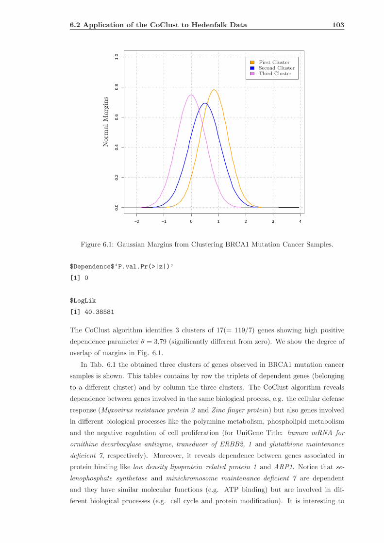
6.2 Application of the CoClust to Hedenfalk Data 103
−2 −1 0 1 2 3 4
0.0
0.2
0.4
0.6
0.8
1.0
Nor
mal
Mar
gins
First ClusterSecond ClusterThird Cluster
Figure 6.1: Gaussian Margins from Clustering BRCA1 Mutation Cancer Samples.
$Dependence$‘P.val.Pr(>|z|)’
[1] 0
$LogLik
[1] 40.38581
The CoClust algorithm identifies 3 clusters of 17(= 119/7) genes showing high positive
dependence parameter θ = 3.79 (significantly different from zero). We show the degree of
overlap of margins in Fig. 6.1.
In Tab. 6.1 the obtained three clusters of genes observed in BRCA1 mutation cancer
samples is shown. This tables contains by row the triplets of dependent genes (belonging
to a different cluster) and by column the three clusters. The CoClust algorithm reveals
dependence between genes involved in the same biological process, e.g. the cellular defense
response (Myxovirus resistance protein 2 and Zinc finger protein) but also genes involved
in different biological processes like the polyamine metabolism, phospholipid metabolism
and the negative regulation of cell proliferation (for UniGene Title: human mRNA for
ornithine decarboxylase antizyme, transducer of ERBB2, 1 and glutathione maintenance
deficient 7, respectively). Moreover, it reveals dependence between genes associated in
protein binding like low density lipoprotein–related protein 1 and ARP1. Notice that se-
lenophosphate synthetase and minichromosome maintenance deficient 7 are dependent
and they have similar molecular functions (e.g. ATP binding) but are involved in dif-
ferent biological processes (e.g. cell cycle and protein modification). It is interesting to
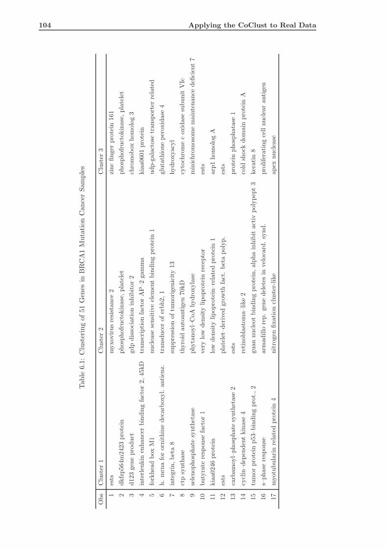
104 Applying the CoClust to Real Data
Tab
le6.
1:C
lust
erin
gof
51G
enes
inB
RC
A1
Muta
tion
Can
cer
Sam
ple
s
Obs
Clu
ster
1C
lust
er2
Clu
ster
3
1es
tsm
yxov
irus
resi
stance
2zi
nc
finger
pro
tein
161
2dkfz
p564m
2423
pro
tein
phosp
hofr
uct
okin
ase
,pla
tele
tphosp
hofr
uct
okin
ase
,pla
tele
t
3d123
gen
epro
duct
gdp
dis
soci
ation
inhib
itor
2ch
rom
obox
hom
olo
g3
4in
terl
eukin
enhance
rbin
din
gfa
ctor
2,45kD
transc
ription
fact
or
AP
–2
gam
ma
kia
a0601
pro
tein
5fo
rkhea
dbox
M1
nucl
ease
sensi
tive
elem
ent
bin
din
gpro
tein
1udp-g
ala
ctose
transp
ort
erre
late
d
6h.
mrn
afo
rorn
ithin
edec
arb
oxyl.
antien
z.tr
ansd
uce
rofer
bb2,1
glu
tath
ione
per
oxid
ase
4
7in
tegri
n,bet
a8
suppre
ssio
noftu
mori
gen
icity
13
hydro
xyacy
l
8ct
psy
nth
ase
thyro
idauto
antigen
70kD
cyto
chro
me
cox
idase
subunit
VIc
9se
lenophosp
hate
synth
etase
phyta
noy
l–C
oA
hydro
xyla
sem
inic
hro
moso
me
main
tenance
defi
cien
t7
10
buty
rate
resp
onse
fact
or
1ver
ylo
wden
sity
lipopro
tein
rece
pto
res
ts
11
kia
a0246
pro
tein
low
den
sity
lipopro
tein
–re
late
dpro
tein
1arp
1hom
olo
gA
12
ests
pla
tele
t–der
ived
gro
wth
fact
.bet
apoly
p.
ests
13
carb
am
oyl–
phosp
hate
synth
etase
2es
tspro
tein
phosp
hata
se1
14
cycl
in–dep
enden
tkin
ase
4re
tinobla
stom
a–like
2co
ldsh
ock
dom
ain
pro
tein
A
15
tum
or
pro
tein
p53–bin
din
gpro
t.,2
guan
nucl
eot
bin
din
gpro
tein
,alp
ha
inhib
itact
ivpoly
pep
t3
ker
atin
8
16
s–phase
resp
onse
arm
adillo
rep.
gen
edel
etes
invel
oca
rd.
synd.
pro
life
rating
cell
nucl
ear
antigen
17
myotu
bula
rin
rela
ted
pro
tein
4nitro
gen
fixation
clust
er-lik
eapex
nucl
ease

6.2 Application of the CoClust to Hedenfalk Data 105
observe that the candidate gene to tumor suppression (suppression of tumorigenicity 13 )
is related to the integrin beta 8 that mediates cell–cell and cell–extracellular interactions.
Moreover cyclin–dependent kinase 4, retinoblastoma–like 2 and Cold shock domain pro-
tein A are dependent according to the overlap of the biological processes in which they are
involved two at time (the cell cycle, division and proliferate, the regulation of progression
through cell cycle and the regulation of transcript DNA–dependent). This result reveals
that the negative regulation of transcription from RNA polymerase II promoter and of
progression through cell cycle are likely to be mutually related, that is, any process that
stops, prevents or reduces the frequency, rate or extent of transcription from an RNA poly-
merase II promoter is related to processes that stop, prevent or reduce the rate or extent
of progression through the cell cycle. Finally, notice that the nitrogen fixation cluster–
like is dependent on the APEX nuclease; namely, it could be possible that the cellular
respiration is an important process for the DNA repair, the regulation of DNA binding
and the transcription from RNA polymerase II promoter. We conclude by observing that
in a same cluster, the CoClust has grouped genes with similar molecular and biological
functions. See, for example, Chromobox homolog 3, Cold shock domain protein A and
Minichromosome maintenance deficient 7 that modulate the frequency, rate or extent of
DNA-dependent transcription and all they are components of the nucleus.
As regards the BRCA2 mutation samples, the CoClust algorithm gives the following
output:
$Number_of_Clusters
[1] 5
$Index.Matrix
[,1] [,2] [,3] [,4] [,5]
[1,] 7 12 26 34 40
[2,] 19 20 16 23 14
[3,] 11 17 29 51 45
[4,] 10 32 37 39 44
[5,] 18 13 15 21 35
[6,] 8 9 22 42 47
[7,] 1 36 5 43 48
[8,] 24 2 28 46 49
[9,] 25 27 6 4 41
[10,] 31 30 3 38 50
$Clustering.Vector
[1] 1 2 3 4 3 3 1 1 2 1 1 2 2 5 3 3 2 1 1 2 4 3 4 1 1 3 2 3 3 2 1 2
0 4 5 2 3 4 4 5 5 4 4 5 5 4 5 5 5 5 4

106 Applying the CoClust to Real Data
$Data_Clusters
Cluster1 Cluster2 Cluster3 Cluster4 Cluster5
[1,] -0.6733446 -0.1278334 0.10436002 0.35065687 1.0851893
[2,] -0.9675840 -0.3011051 0.12221763 0.41210965 1.3584092
[3,] -1.4271164 -0.2484614 -0.28768207 0.14842001 0.5306283
[4,] -1.6094379 -0.7550226 -0.38566248 -0.18632958 0.6043160
[5,] -1.5141277 -0.5978370 -0.31471074 0.09531018 0.2700271
[6,] -1.3470736 -0.4942963 -0.67334455 -0.03045921 0.4885800
[7,] -0.8675006 -0.2357223 -0.04082199 0.39204209 1.1249296
..... ......... ......... .......... .......... .........
[69,] 0.3506569 -0.1984509 0.1310283 0.4317824 1.534714
[70,] -0.6733446 -0.2107210 0.2231436 0.5007753 1.3711807
$Dependence $Dependence$Param
[1] 3.792002
$Dependence$Std.Err
[1] 0.3680580
$Dependence$‘P.val.Pr(>|z|)’
[1] 0
$LogLik
[1] 69.70692
The CoClust algorithm finds 5 clusters of 10(= 70/7) different genes highlighting 5–
plet of dependent genes with a high value of the dependence parameter θ = 3.79. Notice
that the zero in the clustering vector above indicates a gene left out of the clustering. This
gene has clone ID 366647 (33rd row of the original data set: butyrate response factor 1
(EGF–response factor 1)). We show the degree of overlap of margins in Fig. 6.2. In Tab.
6.2, instead, the clustering of BRCA2 mutation cancer samples is shown: the 5–plet of
dependent genes are presented by row and the clusters by column. We note that trans-
ducer of ERBB2, 1 and zinc finger protein 161 are dependent and involved in the negative
regulation of cell proliferation and cellular defense response, respectively, revealing that
the defense response of a cell interacts with any process that stops, prevents or reduces the
rate or extent of cell proliferation. Moreover, the dependent relationship between tran-
scription factor AP–2 gamma, cytochrome c oxidase and armadillo repeat gene deletes in
velocardiofacial syndrome suggests that the chemical reactions and pathways resulting in
the formation of precursor metabolites (substances from which energy is derived) and the
processes involved in the liberation of energy from these substances interact with any pro-
cess that mediates the transfer of information from one cell to another and they are helped

6.2 Application of the CoClust to Hedenfalk Data 107
−4 −2 0 2 4
0.0
0.2
0.4
0.6
0.8
1.0
1.2
Nor
mal
Mar
gins
First ClusterSecond ClusterThird ClusterFourth ClusterFifth Cluster
Figure 6.2: Gaussian Margins from Clustering BRCA2 Mutation Cancer Samples.
by the armadillo that makes easy the communication between internal and external cellu-
lar environments. Finally, we note that the directed movement of substances, either within
a vesicle or in the vesicle membrane, into, out of or within a cell performed by ARP 1,
homolog A is dependent on the enzymatic release of energy from organic compounds which
either requires oxygen (aerobic respiration) or does not (anaerobic respiration) performed
by Nitrogen fixation cluster–like; moreover it is dependent on the formation or destruction
of chromatin structures (complex of DNA and protein that makes up chromosomes and
are relevant to DNA replication and DNA repair) performed by Chromobox homolog 3.
In the end, we note that the second cluster is homogeneous with respect to the cellular
components since most of its genes are in the nucleus of cell.
As regards the Sporadic cancer samples, the CoClust gives the following output:
$Number_of_Clusters
[1] 5
$Index.Matrix
[,1] [,2] [,3] [,4] [,5]
[1,] 20 31 36 38 39
[2,] 8 9 25 7 13
[3,] 15 14 16 34 35
[4,] 3 27 47 42 44
[5,] 1 11 21 6 5

108 Applying the CoClust to Real Data
Tab
le6.
2:C
lust
erin
gof
51G
enes
inB
RC
A2
Muta
tion
Can
cer
Sam
ple
s
Obs
Clu
ster
1C
luster
2C
luster
3C
luster
4C
luster
5
1cold
shock
dom
ain
protein
Aretin
obla
stom
a–like
2gdp
dis
socia
tio
nin
hib
itor
2tum
or
protein
p53–bin
din
gprot.,
2ests
2nucle
ase
sensit
ive
el.
bin
din
gprot.
1d123
gene
product
integrin
,beta
8ests
suppressio
noftum
orig
enic
ity
13
3hydroxyacyl
ests
guan.
nucle
ot.
bin
din
gprot.
3lo
wdensity
lipoprotein
–rela
ted
protein
1m
yxovir
us
resis
tance
2
4prolife
ratin
gcell
nucle
ar
antig
en
ests
cyclin–dependent
kin
ase
4fo
rkhead
box
M1
myotubula
rin
rela
ted
protein
4
5protein
phosphatase
1apex
nucle
ase
thyroid
autoantig
en
70kD
very
low
density
lipoprotein
receptor
interle
ukin
enhancer
bin
din
gfa
ctor
2,45kD
6phosphofr
uctokin
ase,pla
tele
tphosphofr
uctokin
ase,pla
tele
tm
inic
hrom
osom
em
ain
tenance
deficie
nt
7kia
a0246
protein
udp–gala
ctose
transporter
rela
ted
7keratin
8s–phase
response
transducer
oferbb2,1
carbam
oyl–
phosphate
synthetase
2zin
cfinger
protein
161
8kia
a0601
protein
ests
transcrip
tio
nfa
ctor
AP–2
gam
ma
cytochrom
ec
oxid
ase
subunit
VIc
arm
adillo
rep.
gene
dele
tes
invelo
card.
synd.
9dkfz
p564m
2423
protein
chrom
obox
hom
olo
g3
arp1
hom
olo
gA
h.
mrna
for
ornit
hin
edecarboxyl.
antie
nz.
nit
rogen
fixatio
nclu
ster–like
10
ctp
synthase
phytanoyl–
CoA
hydroxyla
se
glu
tathio
ne
peroxid
ase
4sele
nophosphate
synthetase
pla
tele
t–deriv
ed
grow
th
fact.
beta
poly
p.
Tab
le6.
3:C
lust
erin
gof
51G
enes
inSpor
adic
Can
cer
Sam
ple
s
Obs
Clu
ster
1C
luster
2C
luster
3C
luster
4C
luster
5
1d123
gene
product
ctp
synthase
s–phase
response
sele
nophosphate
synthetase
forkhead
box
M1
2phosphofr
uctokin
ase,pla
tele
tphosphofr
uctokin
ase,pla
tele
tdkfz
p564m
2423
protein
cold
shock
dom
ain
protein
Aapex
nucle
ase
3thyroid
autoantig
en
70kD
suppressio
noftum
orig
enic
ity
13
integrin
,beta
8tum
or
protein
p53–bin
din
gprot.,
2in
terle
ukin
enhancer
bin
din
gfa
c.
2
4glu
tathio
ne
peroxid
ase
4chrom
obox
hom
olo
g3
udp-g
ala
ctose
transporter
rela
ted
kia
a0246
protein
myotubula
rin
rela
ted
protein
4
5keratin
8hydroxyacyl
very
low
density
lipoprotein
receptor
arp1
hom
olo
gA
transducer
oferbb2,1
6guan
nucle
ot
bin
din
gprot.
min
ichrom
osom
em
ain
tenance
deficie
nt
7buty
rate
response
factor
1prolife
ratin
gcell
nucle
ar
antig
en
cyclin–dependent
kin
ase
4
7ests
nit
rogen
fixatio
nclu
ster–like
low
density
lipoprotein
–rela
ted
protein
1phytanoyl–
CoA
hydroxyla
se
myxovir
us
resis
tance
2
8transcrip
tio
nfa
ctor
AP–2
gam
ma
kia
a0601
protein
retin
obla
stom
a–like
2ests
ests
9nucle
ase
sensit
ive
el.
bin
din
gprot.
1protein
phosphatase
1zin
cfinger
protein
161
gdp
dis
socia
tio
nin
hib
itor
2carbam
oyl-phosphate
synthetase
2
10
ests
h.
mrna
for
ornit
hin
edecarboxyl.
antie
nz.
arm
adillo
rep.
gene
dele
tes
invelo
card.
synd.
cytochrom
ec
oxid
ase
subunit
VIc
pla
tele
t–deriv
ed
grow
th
fact.
beta
poly
p.

6.2 Application of the CoClust to Hedenfalk Data 109
[6,] 29 22 33 10 37
[7,] 23 41 51 30 45
[8,] 28 24 12 32 40
[9,] 19 18 48 26 43
[10,] 2 4 49 46 50
$Clustering.Vector
[1] 1 1 1 2 5 4 4 1 2 4 2 3 5 2 1 3 0 2 1 1 3 2 1 2 3 4 2 1 1 4 2 4
3 4 5 3 5 4 5 5 2 4 5 5 5 4 3 3 3 5 3
$Data_Clusters
Cluster1 Cluster2 Cluster3 Cluster4 Cluster5
[1,] -0.03045921 0.13976194 0.23111172 0.05826891 0.30748470
[2,] -0.02020271 0.18232156 0.35767444 0.65752000 0.50077529
[3,] -0.08338161 0.11332869 0.53649337 0.39877612 0.44468582
[4,] -0.19845094 0.13976194 0.43825493 0.26236426 1.03673688
[5,] 0.13976194 0.20701417 0.36464311 0.39877612 0.25464222
..... .......... .......... .......... .......... ..........
[69,] -0.41551544 -0.08338161 0.88789126 0.03922071 0.51282363
[70,] 0.16551444 -0.07257069 -0.04082199 -0.17435339 0.12221763
$Dependence
$Dependence$Param
[1] 4.040684
$Dependence$Std.Err
[1] 0.3879386
$Dependence$‘P.val.Pr(>|z|)’
[1] 0
$LogLik
[1] 71.47647
The algorithm identifies 5 clusters of genes each one with 10(= 70/7) genes and indicates
a high positive dependence parameter (significantly different from zero) (θ = 4.04). The
same number of clusters found for the BRCA2 mutation samples is achieved. Notice the
gene with clone ID 246194 is left out (the seventeenth row of original data matrix: ESTs)
as indicated by the presence of a zero in the clustering vector above. We show the degree
of overlap of margins in figure 6.3.
In Tab. 6.3 the clustering of genes observed for the Sporadic cancer samples is shown.

110 Applying the CoClust to Real Data
−2 −1 0 1 2
0.0
0.5
1.0
1.5
Nor
mal
Mar
gins
First ClusterSecond ClusterThird ClusterFourth ClusterFifth Cluster
Figure 6.3: Gaussian Margins from Clustering Sporadic Cancer Samples.
We note that CoClust reveals a dependence between the glycolysis biological process with
the transcription from RNA polymerase II promoter and the negative regulation of tran-
scription from RNA polymerase (phosphofructokinase, platelet, Cold shock domain protein
A and APEX ), the chromatin assembly (disassembly) and modification with the response
to oxidative stress (Glutathione peroxidase and Chromobox homolog 3 ). The most impor-
tant result is that the Human mRNA for ornithine decarboxylase antienzyme is dependent
on Armadillo; indeed, since the polyamines level increases in cancer cells, it could be im-
portant to observe that a gene involved in the respiration process of a cell is related to the
polyamine metabolism. Moreover, nuclease sensitivity, protein phosphatase I, zinc finger
protein and carbamoyl–phosphate synthetase 2 are dependent each other revealing that the
biological process of the cellular defense response interacts with the response to parasite
and the glycogen metabolism. In the end, notice that the CoClust reveals dependence be-
tween Butyrate response factor 1, Proliferating cell nuclear antigen and Cyclin–dependent
kinase 4 showing that the regulation of the cell cycle, the division and proliferation of
cell and the regulation of mRNA stability are mutually related. Finally, we note that the
clusters are quite homogeneous with respect to the kind of cellular component of each
gene.
By comparing the results obtained in the three different mutations samples, we observe
that the strength of estimated dependence between genes in BRCA1 cancer samples is
equal to that estimated for BRCA2 cancer samples whereas it is less than the value of θ
estimated in Sporadic cancer samples. At the same time, the number of identified clusters

6.2 Application of the CoClust to Hedenfalk Data 111
is the same for the BRCA2 and Sporadic cancer samples (5) while it is different from that
identified for the BRCA1 cancer samples (3).
If we compare the clustering (see tables 6.1, 6.2 and 6.3) we note that the clustering
of BRCA1 and BRCA2 mutations cancer samples have 5 couples of dependent genes in
common. In particular we note that the Cold shock domain protein A and retinoblastoma–
like 2 are dependent in both these two kind of mutation cancer samples and they are
involved in the biological process of the negative regulation of transcription of DNA–
dependent. At the same time, the first gene is involved in the negative regulation of
transcription RNA polymerase II promoter while the second one in the negative regulation
of progression. Moreover, perhaps, the most important thing is to note that the candidate
gene for tumor suppression could be the same for both these kinds of mutations.
The results of BRCA1 and Sporadic cancer samples are totally different except for
the following three cases in which the dependence relationship is the same: carbamoyl–
phosphate synthetase 2 and protein phosphatase 1 ; dkfzp564m2423 protein, phosphofruc-
tokinase, platelet and phosphofructokinase, platelet ; integrin, beta 8 and suppression of
tumorigenicity 13. Maybe these sets of genes are not useful for distinguishing the two kind
of mutations. Remarkably the candidate gene for tumor suppression intervenes for both
these kinds of cancer samples.
Finally, clustering of BRCA2 and Sporadic cancer samples present 10 couples and 1
triple of dependent genes in common. These two clusters are similar. For example, the
Proliferating cell nuclear antigen and Cyclin–dependent kinase 4 are dependent and both
of them are involved in the cell proliferation; cytochrome c oxidase and armadillo repeat
gene deletes in velocardiofacial syndrome are dependent and the first one participates to
the metabolism and production of energy in a cell while the second one regulates the
communication between internal and external environment of a cell. Finally, note that
the candidate gene for tumor suppression intervene for both these kinds of mutations.
In conclusion, we stress that the candidate gene to suppression of tumorigenicity 13 is
dependent on the integrin, beta 8 in all the three clustering (different mutations) obtained.
It could be very important to assess this result because for all three kinds of mutation
there could be one useful gene to suppress the tumor.
6.2.2 Classification of Different Breast Cancer Samples
In this section we investigate the capability of the CoClust algorithm of identifying the
relation between different tumor samples. We use the whole data set of Hedenfalk et
al. (2001) and apply the CoClust to their columns. Notice that we are working on the
log–transformed data and we use a Frank copula function.
The output of the CoClust algorithm is the following:
$Number_of_Clusters
[1] 6
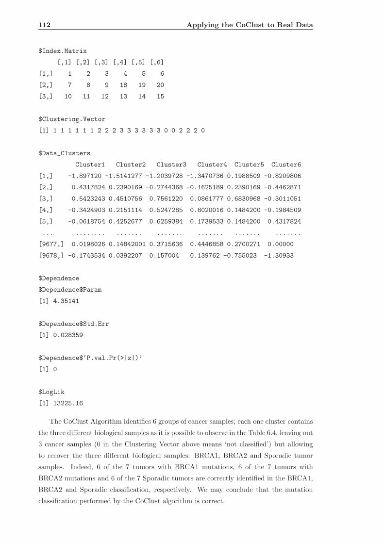
112 Applying the CoClust to Real Data
$Index.Matrix
[,1] [,2] [,3] [,4] [,5] [,6]
[1,] 1 2 3 4 5 6
[2,] 7 8 9 18 19 20
[3,] 10 11 12 13 14 15
$Clustering.Vector
[1] 1 1 1 1 1 1 2 2 2 3 3 3 3 3 3 0 0 2 2 2 0
$Data_Clusters
Cluster1 Cluster2 Cluster3 Cluster4 Cluster5 Cluster6
[1,] -1.897120 -1.5141277 -1.2039728 -1.3470736 0.1988509 -0.8209806
[2,] 0.4317824 0.2390169 -0.2744368 -0.1625189 0.2390169 -0.4462871
[3,] 0.5423243 0.4510756 0.7561220 0.0861777 0.6830968 -0.3011051
[4,] -0.3424903 0.2151114 0.5247285 0.8020016 0.1484200 -0.1984509
[5,] -0.0618754 0.4252677 0.6259384 0.1739533 0.1484200 0.4317824
... ........ ....... ....... ....... ....... .......
[9677,] 0.0198026 0.14842001 0.3715636 0.4446858 0.2700271 0.00000
[9678,] -0.1743534 0.0392207 0.157004 0.139762 -0.755023 -1.30933
$Dependence
$Dependence$Param
[1] 4.35141
$Dependence$Std.Err
[1] 0.028359
$Dependence$‘P.val.Pr(>|z|)’
[1] 0
$LogLik
[1] 13225.16
The CoClust Algorithm identifies 6 groups of cancer samples; each one cluster contains
the three different biological samples as it is possible to observe in the Table 6.4, leaving out
3 cancer samples (0 in the Clustering Vector above means ‘not classified’) but allowing
to recover the three different biological samples: BRCA1, BRCA2 and Sporadic tumor
samples. Indeed, 6 of the 7 tumors with BRCA1 mutations, 6 of the 7 tumors with
BRCA2 mutations and 6 of the 7 Sporadic tumors are correctly identified in the BRCA1,
BRCA2 and Sporadic classification, respectively. We may conclude that the mutation
classification performed by the CoClust algorithm is correct.

6.3 Discussion 113
Table 6.4: Classification of Breast Cancer Mutations by using the CoClust Algorithm
C1 C2 C3 C4 C5 C6
BRCA1 BRCA1 BRCA1 BRCA1 BRCA1 BRCA1
BRCA2 BRCA2 BRCA2 BRCA2 BRCA2 BRCA2
Spor Spor Spor Spor Spor Spor
6.3 Discussion
We have applied the CoClust algorithm to the rows of the microarray data recorded by
of Hedenfalk et al. (2001) for three different observed mutations of cancer samples and to
the columns of the whole data set.
In the first kind of applications, the CoClust algorithm highlights that the candidate
gene for the suppression of tumorigenicity is related to the gene that mediates the cell–cell
and cell–extracell interactions in all three kinds of observed mutations. Furthermore, some
genes have been associated in all three kinds of tumor samples suggesting that they are
not useful for distinguishing the kind of mutation. In addition, the CoClust finds that the
dimension of the dependence is different in the three investigated sets of samples indicating
that perhaps more biological processes are involved in the generation of a BRCA2 or a
Sporadic tumor with respect to BRCA1 mutation tumor. In general, we find that the gene
expressions of BRCA2 mutation cancer samples are more similar to the gene expressions
of Sporadic cancer samples than to those of BRCA1 mutation cancer samples. This could
mean that the genetic background of the patients with sporadic breast cancer may influence
the likelihood of cancer generated by a BRCA2 mutation even in the absence of a specific
predisposing mutation.
The application of the CoClust to the columns of the microarray data set reveals the
capability of the algorithm to classify correctly the three kind of cancer sample. We have
observed that the CoClust does not achieve the correct number of clusters but it is able to
classify correctly the kind of cancer sample clusters composed by the three different kinds
of mutations and relating each kind of them with the same kind of mutation.
We conclude by arguing that the CoClust could be a useful algorithm that allows
to discover new interactions between genes and between the biological processes in which
they are involved, to improve the definition of sporadic cancer case, to distinguish different
cancer samples and to classify new ones.


Conclusions and Perspectives
We have proposed a new clustering algorithm based on copula functions, called ‘CoClust’
in brief (Chapter 5, p. 67). The main purpose was to define a new procedure able to
choose automatically the correct number of clusters and classify observations according
to the underlying dependence structure of the data generating process. Our proposal
originates from the intention to discover clusters of gene expressions according to their
dependence relationship overcoming the limits of other well–known clustering methods
to classify dependent data. The main theory involved in the performed research is that
of copula functions (Chapter 2, p.21). We have studied the performance of the CoClust
algorithm on simulated data and compared it with other clustering techniques (Chapters
4, p. 45 and 5, p. 67). The techniques involved in the comparison were the K–means, the
hierarchical and the model–based clustering methods (Chapter 1, Section 1.2, p. 9). By
using three sets of performance measures (Chapter 4, Section 4.1.3, p. 48) we have shown
that the algorithm proposed outperforms other proposals for the following reasons:
1. it is able to find clusters of observations (e.g., gene expressions or experimental
conditions) according to the dependence structure of the data allowing to recover
the true dependence relationship
- irrespective of the degree of overlap of margins;
- irrespective of the level of dependence between margins;
2. it is not needed to know a priori the true number of clusters since CoClust is always
able to find the true one;
3. it does not require a starting classification;
4. being grounded on copulas, it can virtually account for any possible dependence
relationship between gene expressions; this clearly allows to overcome the limits of
the model–based clustering that tends to use a high number of components/clusters
for modeling non Gaussian data;
5. it allows to discover the k–plets of observations that are reciprocally dependent.
The R code for the ‘CoClust’ function is presented and commented in the Appendix A,
p. 117. Finally, we have applied the proposed algorithm to real microarray data (Chapters
3, p. 33 and Chapter 6, p. 99).
115

116 Applying the CoClust to Real Data
The research performed could be extended in many different directions. First of all,
the proposed algorithm could be tested on non Gaussian margins and on unchangeable
dispersion structure. Second, it would be interesting to introduce a criteria to choose the
best model for copula into the procedure instead of requiring it from the user. Third,
the copula based split up rule (Chapter 5, Section 5.1.2, p. 69) could be involved in the
discriminant analysis for the definition of a new classification rule based on copula mod-
els. Fourth, it could be possible to combine dependence within clusters with dependence
between clusters in order to take into account both the dependence between genes and the
dependence between experiments; this may be achieved by using a combination of copulas
to express the dependence structure.
Furthermore, the CoClust algorithm might be combined or integrated in the context
of model–based clustering techniques in order to avoid the drawbacks that affect the
two and gain further flexibility and power. In fact, one drawback of our proposal is its
computational complexity. Nevertheless, there is room for further optimization of the
algorithm under this aspect and a new faster version is under development.
Another crucial aspect lies in the fact that the CoClust finds clusters of equal size
leaving out a number of observations varying between 1 and k − 1, where k is the num-
ber of identified clusters. This limit could be overcome introducing the estimation of a
conditional copula function that allows to identify genes dependent from other genes but
not necessarily from a gene in each identified cluster, that is, it allows us to keep in con-
sideration if a new observation can belong to a cluster without any other corresponding
observation in other clusters.
An interesting future application could be to use CoClust not to group gene expression
patterns but summary statistics, e.g. the t–statistics. In the end, it would be very
interesting to investigate whether the CoClust could suggest a solution for the important
matter of the dependence between the p–values in multiple tests used to discover genes
differentially expressed.
Finally, we stress that the proposed algorithm opens the door to a new way of inter-
preting clustering techniques and that it can be applied to all the fields in which clustering
dependent data is of interest.

Appendix A: CoClust R Code
The R code for the Copula–based algorithm requires the following packages:
library(copula) # to define and estimate copula function
library(gtools) # to compute dispositions
The R code for the Copula–based algorithm is the following:
CoClust <- function(m,nmaxmarg=6,copula){ # m: data matrix of
# dimension n.row*n.col
# nmaxmarg: maximum number
# of clusters to try
# copula: kind of model
# for copula
n.row <- dim(m)[1]; # rows num. of data matrix in input
# (e.g. number of genes)
n.col <- dim(m)[2]; # cols num. of data mtrix in entry
# (e.g. num. of experimental conditions)
loglik.marg <- function(b,y) sum(dnorm(y,mean=b[1],sd=b[2],
log=TRUE));
# function of maxloglik for margins
ctrl <- list(fnscale=-1); # parameter of maximization
ifelse(n.row <= nmaxmarg, dimc <- n.row, dimc <- nmaxmarg);
# condition to avoid that the max dimension
# of copula is greater than the rows (obs) number
llikm <- vector(length=(dimc-1)); # vector of the selected
# maxloglik for each
# copula of different
# dimension (to choose
# the number of
# clusters)
clusters <- list()
clusters[[1]] <- ("max ML by varying the number of clusters");
# initialization of the list of the first
# h-plet of obs selected by varying of the
117
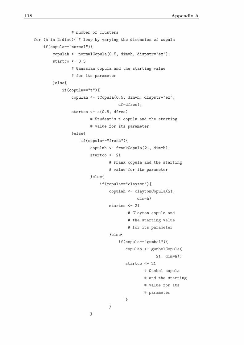
118 Appendix A
# number of clusters
for (h in 2:dimc){ # loop by varying the dimension of copula
if(copula=="normal"){
copulah <- normalCopula(0.5, dim=h, dispstr="ex");
startco <- 0.5
# Gaussian copula and the starting value
# for its parameter
}else{
if(copula=="t"){
copulah <- tCopula(0.5, dim=h, dispstr="ex",
df=dfree);
startco <- c(0.5, dfree)
# Student’s t copula and the starting
# value for its parameter
}else{
if(copula=="frank"){
copulah <- frankCopula(21, dim=h);
startco <- 21
# Frank copula and the starting
# value for its parameter
}else{
if(copula=="clayton"){
copulah <- claytonCopula(21,
dim=h)
startco <- 21
# Clayton copula and
# the starting value
# for its parameter
}else{
if(copula=="gumbel"){
copulah <- gumbelCopula(
21, dim=h);
startco <- 21
# Gumbel copula
# and the starting
# value for its
# parameter
}
}
}
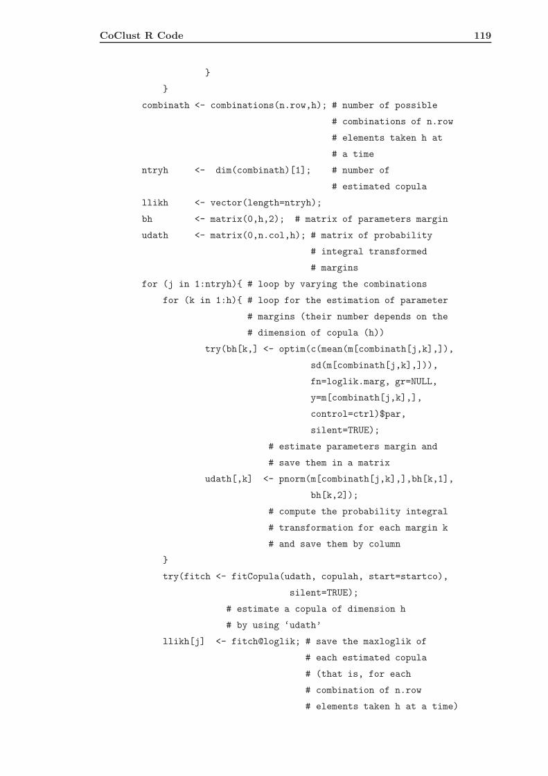
CoClust R Code 119
}
}
combinath <- combinations(n.row,h); # number of possible
# combinations of n.row
# elements taken h at
# a time
ntryh <- dim(combinath)[1]; # number of
# estimated copula
llikh <- vector(length=ntryh);
bh <- matrix(0,h,2); # matrix of parameters margin
udath <- matrix(0,n.col,h); # matrix of probability
# integral transformed
# margins
for (j in 1:ntryh){ # loop by varying the combinations
for (k in 1:h){ # loop for the estimation of parameter
# margins (their number depends on the
# dimension of copula (h))
try(bh[k,] <- optim(c(mean(m[combinath[j,k],]),
sd(m[combinath[j,k],])),
fn=loglik.marg, gr=NULL,
y=m[combinath[j,k],],
control=ctrl)$par,
silent=TRUE);
# estimate parameters margin and
# save them in a matrix
udath[,k] <- pnorm(m[combinath[j,k],],bh[k,1],
bh[k,2]);
# compute the probability integral
# transformation for each margin k
# and save them by column
}
try(fitch <- fitCopula(udath, copulah, start=startco),
silent=TRUE);
# estimate a copula of dimension h
# by using ‘udath’
llikh[j] <- fitch@loglik; # save the maxloglik of
# each estimated copula
# (that is, for each
# combination of n.row
# elements taken h at a time)
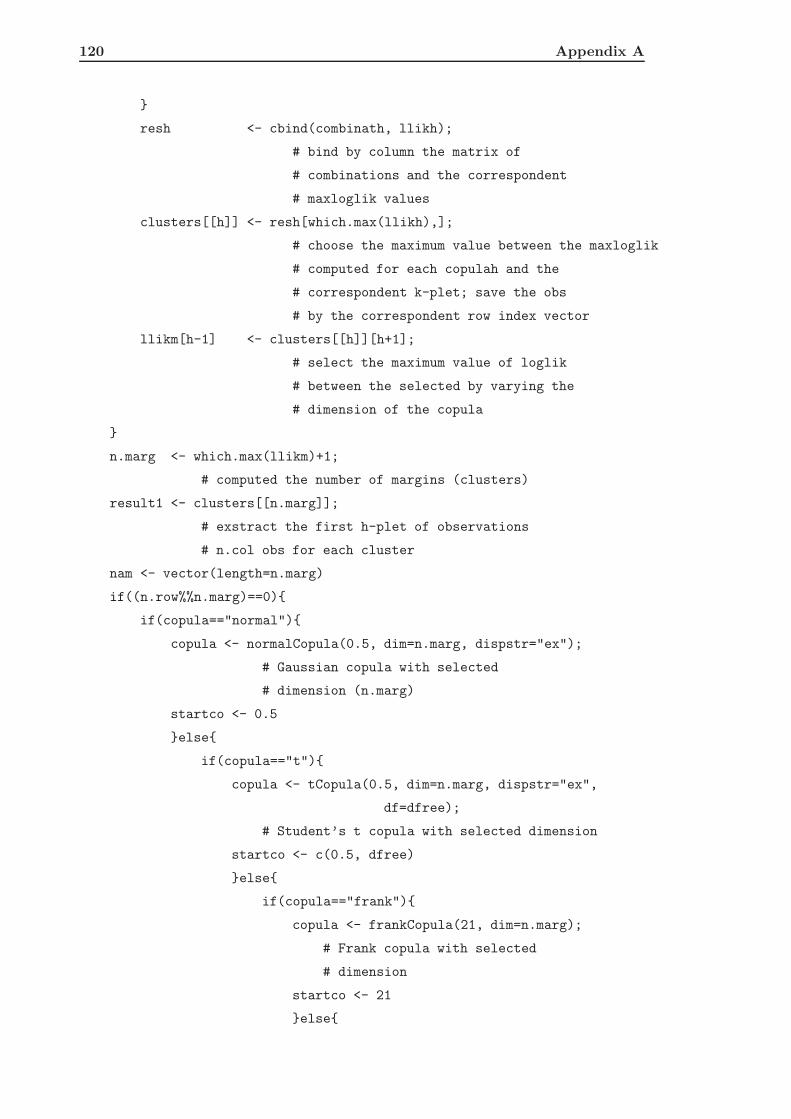
120 Appendix A
}
resh <- cbind(combinath, llikh);
# bind by column the matrix of
# combinations and the correspondent
# maxloglik values
clusters[[h]] <- resh[which.max(llikh),];
# choose the maximum value between the maxloglik
# computed for each copulah and the
# correspondent k-plet; save the obs
# by the correspondent row index vector
llikm[h-1] <- clusters[[h]][h+1];
# select the maximum value of loglik
# between the selected by varying the
# dimension of the copula
}
n.marg <- which.max(llikm)+1;
# computed the number of margins (clusters)
result1 <- clusters[[n.marg]];
# exstract the first h-plet of observations
# n.col obs for each cluster
nam <- vector(length=n.marg)
if((n.row%%n.marg)==0){
if(copula=="normal"){
copula <- normalCopula(0.5, dim=n.marg, dispstr="ex");
# Gaussian copula with selected
# dimension (n.marg)
startco <- 0.5
}else{
if(copula=="t"){
copula <- tCopula(0.5, dim=n.marg, dispstr="ex",
df=dfree);
# Student’s t copula with selected dimension
startco <- c(0.5, dfree)
}else{
if(copula=="frank"){
copula <- frankCopula(21, dim=n.marg);
# Frank copula with selected
# dimension
startco <- 21
}else{

CoClust R Code 121
if(copula=="clayton"){
copula <- claytonCopula(21,
dim=n.marg)
# Clayton copula with
# selected dimension
startco <- 21
}else{
if(copula=="gumbel"){
copula <- gumbelCopula(21,
dim=n.marg);
# Gumbel copula with
# selected dimension
startco <- 21
}
}
}
}
}
noc <- n.row/n.marg;
# number of oservations (e.g. gene
# expressions) for each cluster
result <- matrix(0,noc,n.marg);
# matrix of row index of observations
# grouped in n.marg clusters
result[1,] <- result1[1:n.marg];
# introduce in the first row the row indexes
# of the first selected h-plet of obs
mfin <- matrix(0,(noc*n.col),n.marg);
# matrix of clustered data
udat <- matrix(0,(noc*n.col),n.marg);
# matrix of probability integral
# transform for each margin
bfin <- matrix(0,n.marg,2);
# matrix of estimated parameters margin
datprec <- vector(length=n.marg);
for (j in 1:n.marg){
mfin[1:n.col,j] <- m[result[1,j],];
# matrix of clustered obs
datprec[j] <- result[1,j];
# save the first selected h-plet of rows

122 Appendix A
# (that is, its row indexes)
}
res <- c(1:n.row)[-datprec];
# vector of remaining rows (G-n.marg)
# on which to compute the dispositions
for (i in 2:noc){
combinat <- permutations((n.row-(n.marg*(i-1))),
n.marg,res);
# matrix of dispositions of remaining
# row indexes taken n.marg at a time
ntry <- dim(combinat)[1];
# number of estimated copulas
# (numbers of computed dispositions)
logl <- vector(length=ntry);
# vector of the maxloglik for each
# computed disposition
for (j in 1:ntry){
# loop by varying the dispositions
for (k in 1:n.marg){
# loop by varying margins
try(bfin[k,] <- optim(
c(mean(c(mfin[(1:(n.col*(i-1))),k],
m[combinat[j,k],])),
sd(c(mfin[(1:(n.col*(i-1))),k],
m[combinat[j,k],]))), fn=loglik.marg,
gr=NULL, y=c(mfin[(1:(n.col*(i-1))),k],
m[combinat[j,k],]), control=ctrl)$par,
silent=TRUE);
# estimate of parameters margins
udat[1:(n.col*i),k] <- pnorm(
c(mfin[(1:(n.col*(i-1))),k],
m[combinat[j,k],]),bfin[k,1],
bfin[k,2]);
# compute the probability
# integral transformation for margins
}
try(fitc <- fitCopula(udat[1:(n.col*i),1:n.marg], copula,
start=startco), silent=TRUE);
# estimate a copula function for each disposition
logl[j] <- fitc@loglik;

CoClust R Code 123
# save the values of maxloglik of estimated copulas
# for each disposition
}
res2 <- cbind(combinat, logl);
# link in column the matrix of dispositions
# with the computed maxloglik
result2 <- res2[which.max(logl),];
# select the maximum value among the
# computed maxloglik
result[i,] <- result2[1:n.marg];
# introduce (by row) the row indexes of the
# i-th vector of selected observations
for (j in 1:n.marg){
# loop to update ‘res’
# (remaining row indexes)
mfin[((i-1)*n.col+1):(i*n.col),j] <- m[result[i,j],];
# matrix of clustered obs (rows of m)
datprec[j] <- which(res==result[i,j]);
# select the indexes of
# the new clustered observations
}
res <- res[-datprec];
# updated the vector of remaining row indexes
}
b1 <- matrix(0,n.marg,2)
# from here onward: estimate the copula on clustered data
# and save the output
for(j in 1:n.marg){
# loop by varying the number of margins
for(i in 1:noc){
# loop by varying number of observations
# in each cluster
m[result[i,j],1] <- j
clustering.vector <- m[,1]
# return a vector of integers indicating
# the cluster to which each point
# is allocated
}
nam[j] <- paste("Cluster",j,sep="")
# return the name of the columns of mfin

124 Appendix A
colnames(mfin) <- nam
try(b1[j,] <- optim(c(mean(mfin[,j]),sd(mfin[,j])),
fn=loglik.marg, gr=NULL,
y=mfin[,j], control=ctrl)$par,
silent=TRUE)
# estimate parameters margins
udat[,j] <- pnorm(mfin[,j],b1[j,1],b1[j,2])
# compute the probability integral
# transformation of each margin
}
try(fitfin <- fitCopula(udat, copula,
start=startco), silent=TRUE);
# estimate copula function on
# clustered data
depfin <- c(Param=fitfin@est,
Std.Err=sqrt([email protected]),
P.val=summary(fitfin)@parameters[4]);
# save the analysis of dependence
# between clustered data
return(list(Number_of_Clusters=n.marg, Index.Matrix=result,
Clustering.Vector=clustering.vector, Data_Clusters=mfin,
Dependence=depfin, LogLik=fitfin@loglik));
# return: the number of clusters, the matrix of
# row indexes, the vector of allocation indexes,
# the matrix of clustered data, the results
# of the analysis of dependence and
# the estimated loglik copula function
}
else {print("No possible clustering")}
# output whether the ‘if’ is not verified
}
Notice that if a Student t copula is chosen, then the degrees of freedom have to be define
before of applying the function ‘Coclust’.
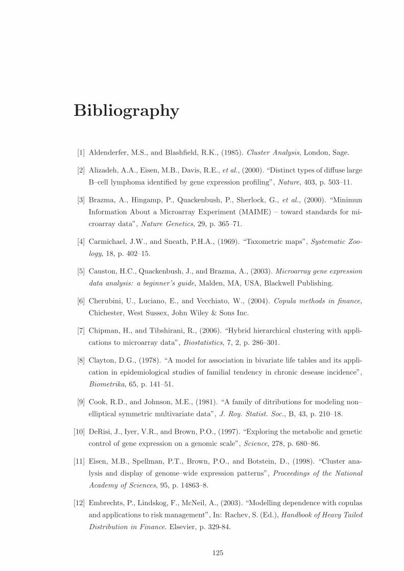
Bibliography
[1] Aldenderfer, M.S., and Blashfield, R.K., (1985). Cluster Analysis, London, Sage.
[2] Alizadeh, A.A., Eisen, M.B., Davis, R.E., et al., (2000). “Distinct types of diffuse large
B–cell lymphoma identified by gene expression profiling”, Nature, 403, p. 503–11.
[3] Brazma, A., Hingamp, P., Quackenbush, P., Sherlock, G., et al., (2000). “Minimun
Information About a Microarray Experiment (MAIME) – toward standards for mi-
croarray data”, Nature Genetics, 29, p. 365–71.
[4] Carmichael, J.W., and Sneath, P.H.A., (1969). “Taxometric maps”, Systematic Zoo-
logy, 18, p. 402–15.
[5] Causton, H.C., Quackenbush, J., and Brazma, A., (2003). Microarray gene expression
data analysis: a beginner’s guide, Malden, MA, USA, Blackwell Publishing.
[6] Cherubini, U., Luciano, E., and Vecchiato, W., (2004). Copula methods in finance,
Chichester, West Sussex, John Wiley & Sons Inc.
[7] Chipman, H., and Tibshirani, R., (2006). “Hybrid hierarchical clustering with appli-
cations to microarray data”, Biostatistics, 7, 2, p. 286–301.
[8] Clayton, D.G., (1978). “A model for association in bivariate life tables and its appli-
cation in epidemiological studies of familial tendency in chronic desease incidence”,
Biometrika, 65, p. 141–51.
[9] Cook, R.D., and Johnson, M.E., (1981). “A family of ditributions for modeling non–
elliptical symmetric multivariate data”, J. Roy. Statist. Soc., B, 43, p. 210–18.
[10] DeRisi, J., Iyer, V.R., and Brown, P.O., (1997). “Exploring the metabolic and genetic
control of gene expression on a genomic scale”, Science, 278, p. 680–86.
[11] Eisen, M.B., Spellman, P.T., Brown, P.O., and Botstein, D., (1998). “Cluster ana-
lysis and display of genome–wide expression patterns”, Proceedings of the National
Academy of Sciences, 95, p. 14863–8.
[12] Embrechts, P., Lindskog, F., McNeil, A., (2003). “Modelling dependence with copulas
and applications to risk management”, In: Rachev, S. (Ed.), Handbook of Heavy Tailed
Distribution in Finance. Elsevier, p. 329-84.
125

126 Bibliography
[13] Escarela, G., and Carriere, J.F., (2003). “Fitting competing risks with an assumed
copula”, Statistical Methods in Medical Research, 12, 4, p. 333-49.
[14] Everitt, B., (1993). Cluster Analsys (Third Edition), London, E. Arnold, New York,
Halsted Press.
[15] Ewens, W.J., and Grant, G.R., (2005). Statistical Methods in Bioinformatics. An
Introduction, (Second Edition), New York, USA, Springer.
[16] Florek, K., Lukaszewiez, J., et al., (1951). “Sur la liason et la division des points d’un
ensemble fini”, Colloquium Mathematicum, 2, p. 282–5.
[17] Fraley, C., and Raftery, E., (1998). “How Many Clusters? Which Clustering Method?
Answers Via Model–Based Cluster Analysis”, The Computer Journal, vol. 41, n. 8,
p. 578–88.
[18] Fraley, C., and Raftery, E., (1999). “MCLUST: Software for model–based cluster
analysis”, J. Classification, vol. 16, p. 297-306.
[19] Fraley C., and Raftery, A.E., (2000). “Model–based Clustering Discirminat Analy-
sis and, Density Estimation”, Technical Report no. 380, Department of Statistics,
University of Washington, p. 1–48.
[20] Fraley C., and Raftery, A.E., (2007). “Model–based Methods of Classifications: Using
the mclust Software in Chemometrics”, Journal of Statistical Software, vol. 18, issue
6, p. 1–13.
[21] Frank, M.J., (1979). “On the simultaneous associativity of F(x,y) and x+y-F(x,y)”,
Aequationes Math, 19, p. 194–226.
[22] Frechet, M., (1951). “Sur les tableaux de correlation dont les marges sont donnees”,
Ann Univ Lyon, Sec A, 9, p. 53–77.
[23] Frees, E.W., Carriere, J., Valdez, E.A., (1996). “Annuity valuation with dependent
mortality”, Journal of Risk and Insurance, 63, p. 229-61.
[24] Frees, E.W., and Valdez, E.A., (1998). “Understanding relationships using copulas”,
North American Actuarial Journal, 2, 1, p. 1-25.
[25] Frees, E.W., and Wang, P., (2005). “Credibility using copulas”, North American
Actuarial Journal, 9, 2, p. 31-48.
[26] Friedman, N., Linial, m., Nachman, I. and Pe’er, D., (2000). “Using Bayesian networks
to analyze expression data”, Journal of Computational Biology, 7, 3, p. 601–20.
[27] Getz, G., Levine, E., and Domany, E. (2000). “Coupled Two–Way Clustering Analysis
of Gene Microarray Data”. Proc. Natural Academy of Sciences US, p. 12079–84.

Bibliography 127
[28] Godambe, V. P., (1960). “An optimum property of regular maximum likelihood esti-
mation”, Ann. of Math. Statist., 31, p. 1208–11.
[29] Gumbel, E.J., (1960). “Bivariate exponential distributions”, J. Amer. Statist. Assoc.,
55, p. 698–707.
[30] Hartigan, J.A., (1972). “Direct Clustering of a Data Matrix”. J. Am. Statistical Assoc.
(JASA), 67, 337, p. 123–9.
[31] Hartigan, J.A., (1975). Clustering algorithms, New York, USA, Wiley.
[32] Hartigan, J.A., and Wong, M.A., (1979). “Algorithm AS 136: A K–Means Clustering
Algorithm”, Applied Statistics, 28, 1, p. 100–8.
[33] Hedenfalk, I., Duggan, D., et al., (2001). “Gene–Expression Profiles in Hereditary
Breast Cancer”, The New England Journal of Medicine, 344, 8, p. 539–48.
[34] Herrero, J., Valencia, A., and Dopazo, J., (2001). “A hierarchical unsupervised grow-
ing neural network for clustering gene expression patterns”. Bioinformatics, vol. 17,
p. 126-36.
[35] Joe, H., and Xu, J., (1996). “The estimation method of inference functions for margins
for multivariate models”, Technical Report, 166, Department of Statistics, University
of British Columbia.
[36] Joe, H., (1997). Multivariate Models and Multivariate Concepts, New York, Chapman
& Hall.
[37] Johnson, S.C., (1967). “Hierarchical clustering schemes”, Psychometrica, 32, p. 241–
54.
[38] Johnson, N.L., and Kotz, S., (1972). Distributions in Statistics: Continuous Multi-
variate Distributions, New York, Wiley.
[39] Kaufman, L., and Rousseeuw, P.J., (1990). Finding Groups in Data: an introduction
to Cluster Analysis, New York, J. Wiley & Sons.
[40] Kimeldorf, G., and Sampson, A., (1975a). “One–parameter families of bivariate distri-
butions with fixed marginals”, Comm. Statist. A – Theory Methods, 4, p. 293–301.
[41] Kimeldorf, G., and Sampson, A., (1975b). “Uniform representations of bivariate dis-
tributions”, Comm. Statist. A – Theory Methods, 4, p. 617–23.
[42] Knudsen, S., (2004). Guide to Analysis of DNA Microarray Data, (second edition),
Hoboken, New Jersey, John Wiley & Sons Inc.
[43] Kohonen, T., (1990). “The self–organizing map”, Proc. IEEE, 48, p. 1464-79.

128 Bibliography
[44] Lance, G.N., and Williams, W.T., (1979). “INVER: A program for the computation of
distance–measures between attributes of mixed types”, Australian Computer Journal,
11, p. 27–8.
[45] Lee, M.-L.T., (2004). Analysis of microarray gene expression data, Boston, MA, USA,
Kluwer Academic Publishers.
[46] Li, M., Boehnke, M., Abecasis, G.R., and Song, X.–K.P., (2006), “Quantitative Trait
Linkage Analysis Using Gaussian Copulas”, Genetics, 173, p. 2371–27.
[47] MacQueen, J., (1967). “Some methods for classification and analysis of multivariate
observations”, 4th Berkeley Symp. Math. Statist. Prob., edited by L. Le Cam and J.
Neyman, 1, p. 281–97.
[48] Madeira, S.C., and Oliveira, A.L., (2004). “Biclustering Algorithms for Biological
Data Analisys: a Survey”, IEEE. TRANSACTIONS ON COMPUTATIONAL BIO-
LOGY AND BIOINFORMATICS, 1(1), p. 24–45.
[49] McLachlan, G.J., Do, K.–A., and Ambroise, C., (2004). Analyzing microarray gene
expression data, Hoboken, N.J., Wiley–Interscience.
[50] Moreaou, Y., De Smet, F., Thijs, G., Marchal, K. and De Moor, B., (2002). “Func-
tional Bioinformatics of Microarray Data: From Expression to Regulation”, Procee-
dings of the IEEE, 90, 11, p. 1722–43.
[51] Morgenstern, D., (1956). “Einfache Beispiele Zweidimensionaler Verteilungen”, Mitt.
Math. Statist., 8, p. 234–5.
[52] Nelsen, R.B., (2006). Introduction to copulas, New York, Springer.
[53] Nuber, U.A., (2005). DNA microarrays, Advanced Methods, New York, Taylor &
Francis Group.
[54] Owzar, K., Jung, S-H, and Sen, P.K., (2007). “A Copula Approach for Detecting
Prognostic Genes Associated With Survival Outcome in Microarray Studies”, Bio-
metrics, 63, p. 1089–98.
[55] Pa, W., Lin, J., and Le, T.C., (2002). “Model–based cluster of analysis of microarray
gene–expression data”, Genome Biology, 3, 2, research0009.1-0009.8.
[56] Schena, M., Shalon, D., David, R.W., and Brown, P.O., (1995). “Quantitative moni-
toring of gene expression patterns with a complementary DNA microarray”, Science,
270, p. 467–70.
[57] Serfling, R.J., (1980). Approximation Theorems of Mathematical Statistics. John Wi-
ley & Sons, New York.
[58] Shao, J., (1999). Mathematical Statistics. Springer-Verlag, New York.

Bibliography 129
[59] Sklar, A., (1959). “Fonctions de repartition a n dimensions et leures marges”, Publi-
cations de l’Institut de Statistique de L’Universite de Paris, 8, p. 229–31.
[60] Sneath, P.H.A., (1957). “The application of computers to taxonomy”, J. Gen. Mi-
crobiol., 17, p. 201–26.
[61] Sørlie, T., Perou, C.M., Tibshirani, R., Aas, T., et al., (2001). “Gene expression
patterns of breast carcinomas distinguish tumor subclasses with clinical implications”,
Proceedings of the National Academy of Sciences of the United States of America, 98,
p. 10869–74.
[62] Speed, T., (2003). Statistical Analysis of Gene Expression Microarray Data, Chapman
& Hall, New York.
[63] Stekel, D., (2003). Microarray Bioinformatics, Cambridge University Press.
[64] Tamayo, P., Slonim, D., Mesirov, J., Zhu, Q., Kitareewan, S., Dmitrovsky, E., Lander,
E.S., and Golub, T.R., (1999). “Interpreting patterns of gene expression with self–
organizing maps: methods and application to hematopoietic differentiation”, Proc.
Nat. Acad. Sci. USA, 96, p. 2907-12.
[65] Tavazoie, S., Hughes, J.D., Campbell, M.J., Cho, R.J., and Church, G.M, (1999).
“Systematic determination of genetic network architecture”, Nat. Gent., 22(3),
p. 281–5.
[66] Tregouet, D.–A., Ducimetiere, P., Bocquet, V., Visvikis, S., Soubrier, F., and Tiret,
L., (1999). “A Parametric Copula Model for Analysis of Familial Binary Data”. Am.
J. Hum. Genet., 64, p. 886-93.
[67] Trivedi, P.K., and Zimmer, D.M., (2007). Copula Modeling: An Introduction for
Practitioners, Now Publishers.
[68] Wang, W., and Wells, M.T., (2000). ”Model selection and semiparametric inference
for bivariate failure-time data” (C/R: p73-76), Journal of the American Statistical
Association, 95, 449, p. 62-72.
[69] Watson, J.D., and Crick, F.H.C., (1953). “Molecular Structure of Nucleic Acids”,
Nature, 3, 171, p. 737–8.
[70] Wit, E., and McClure, J., (2004). Statistics for microarray, Chichester, West Sussex,
John Wiley & Sons Inc.
[71] Yan, J., (2006). “Enjoy the Joy of Copulas”, Preprint submitted to Journal of Stati-
stical Software, p. 1–20.
[72] Yan, J., (2006). “Multivariate modeling with copulas and engineering applications”,
In: Pham, H. (Ed.), Handbook in Engineering Statistics. Springer, p. 973-90.

130 Bibliography
[73] Yeung, K.Y., Fraley, C., Murua, A., Raftery, A.E., and Ruzzo, W.L., (2001). “Model–
based clustering and data transformation for gene expression data”, Bioinformatics,
17(10), p. 977–87.