Analyzing iterated learning Tom Griffiths Brown University Mike Kalish University of Louisiana.

Analyzing iterated learning

Tom GriffithsBrown University

Mike KalishUniversity of Louisiana

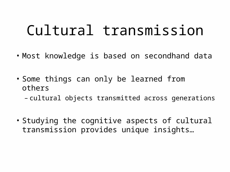
Cultural transmission

• Most knowledge is based on secondhand data

• Some things can only be learned from others– cultural objects transmitted across generations

• Studying the cognitive aspects of cultural transmission provides unique insights…

Iterated learning(Kirby, 2001)

• Each learner sees data, forms a hypothesis, produces the data given to the next learner

• c.f. the playground game “telephone”

QuickTime™ and aTIFF (LZW) decompressor

are needed to see this picture.

Objects of iterated learning

• It’s not just about languages…

• In the wild:– religious concepts– social norms– myths and legends– causal theories

• In the lab:– functions and categories

Outline

1. Analyzing iterated learning

2. Iterated Bayesian learning

3. Examples

4. Iterated learning with humans

5. Conclusions and open questions

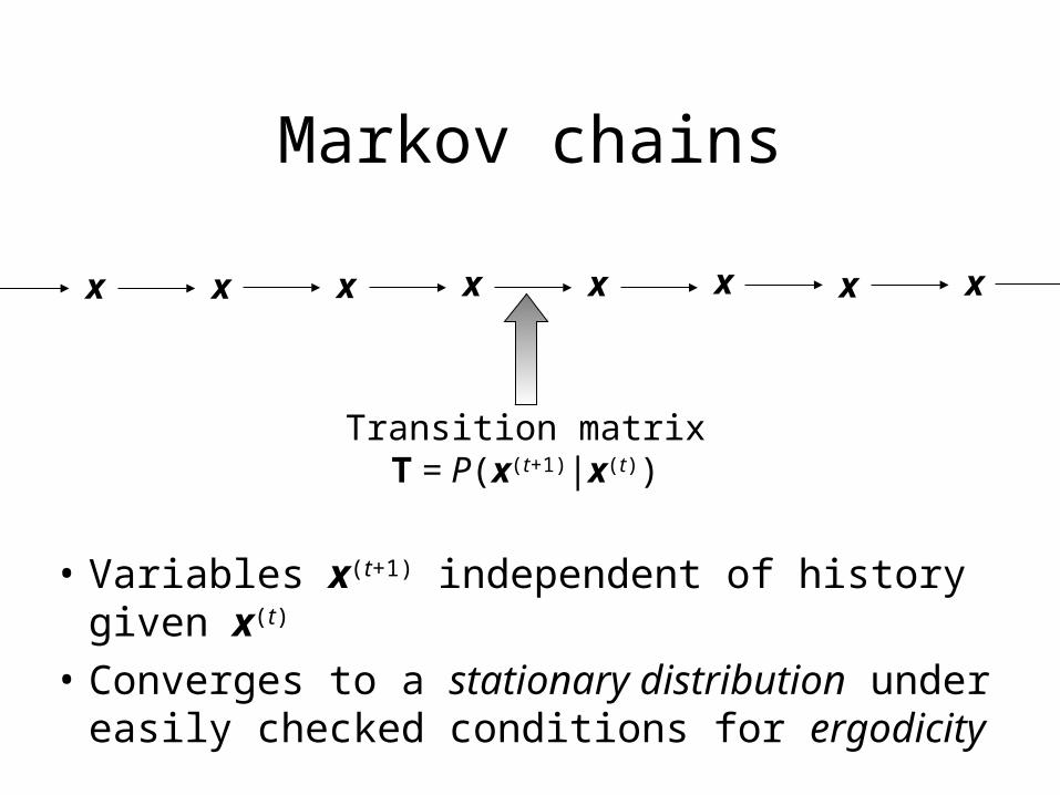
• Variables x(t+1) independent of history given x(t)

• Converges to a stationary distribution under easily checked conditions for ergodicity

x x x x x x x x

Transition matrixT = P(x(t+1)|x(t))

Markov chains

Stationary distributions

• Stationary distribution:

• In matrix form

is the first eigenvector of the matrix T

• Second eigenvalue sets rate of convergence

€

i = P(x(t +1) = i |j

∑ x(t ) = j)π j = Tijπ j

j

∑

€

=Tπ

A Markov chain on hypotheses

• Transition probabilities sum out data

• Stationary distribution and convergence rate from eigenvectors and eigenvalues of Q– can be computed numerically for matrices of

reasonable size, and analytically in some cases

€

Qij = P(hn +1 = i | hn = j) = P(hn +1 = i |d

∑ d) P(d | hn = j)

Infinite populations in continuous time

• “Language dynamical equation”

• “Neutral model” (fj(x) constant)

• Stable equilibrium at first eigenvector of Q

€

dx i

dt= Qij f j (x)

j

∑ x j − φ(x)x i

(Nowak, Komarova, & Niyogi, 2001)

€

dx i

dt= Qij

j

∑ x j − x i

(Komarova & Nowak, 2003)

€

dx

dt= (Q − I)x

Outline



3. Examples



Bayesian inference

QuickTime™ and aTIFF (Uncompressed) decompressor


Reverend Thomas Bayes

• Rational procedure for updating beliefs

• Foundation of many learning algorithms

(e.g., Mackay, 2003)

• Widely used for language learning

(e.g., Charniak, 1993)

Bayes’ theorem

€

P(h | d) =P(d | h)P(h)

P(d | ′ h )P( ′ h )′ h ∈H

∑

Posteriorprobability

Likelihood Priorprobability

Sum over space of hypothesesh: hypothesis

d: data

Iterated Bayesian learning







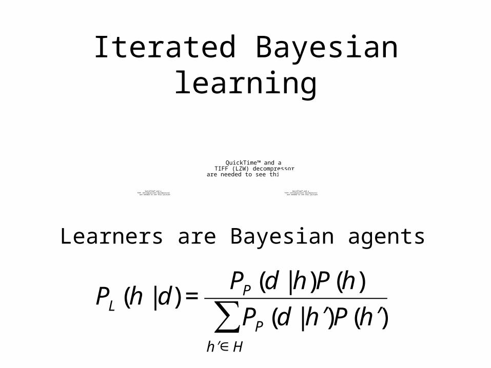
Learners are Bayesian agents

€

PL (h | d) =PP (d | h)P(h)

PP (d | ′ h )P( ′ h )′ h ∈H

∑

Markov chains on h and d

• Markov chain on h has stationary distribution

• Markov chain on d has stationary distribution

€

i = P(h = i) the prior

€

i = PP (d = i | h)h

∑ P(h)the prior

predictivedistribution

Markov chain Monte Carlo

• A strategy for sampling from complex probability distributions

• Key idea: construct a Markov chain which converges to a particular distribution– e.g. Metropolis algorithm– e.g. Gibbs sampling

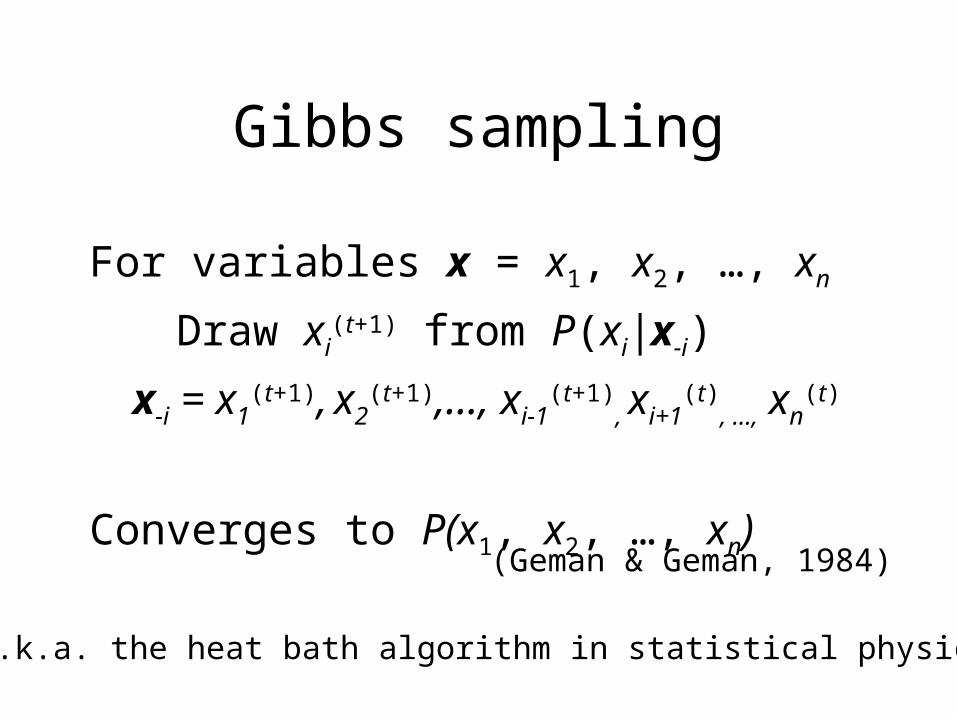
Gibbs sampling

For variables x = x1, x2, …, xn

Draw xi(t+1) from P(xi|x-i)

x-i = x1(t+1), x2

(t+1),…, xi-1(t+1)

, xi+1(t)

, …, xn(t)

Converges to P(x1, x2, …, xn)

(a.k.a. the heat bath algorithm in statistical physics)

(Geman & Geman, 1984)

Gibbs sampling

(MacKay, 2003)

Iterated learning is a Gibbs sampler

• Iterated Bayesian learning is a sampler for

• Implies:– (h,d) converges to this distribution– converence rates are known

(Liu, Wong, & Kong, 1995)€

p(d,h) = p(d | h) p(h)

Outline



3. Examples



An example: Gaussians

€

μn =xn /σ x

2 + μ0 /σ 02

1/σ x2 +1/σ 0

2

€

σ n2 =

1

1/σ x2 +1/σ 0

2

• If we assume…– data, d, is a single real number, x– hypotheses, h, are means of a Gaussian, μ– prior, p(μ), is Gaussian(μ0,σ0

2)

• …then p(xn+1|xn) is Gaussian(μn, σx2 + σn

2)


• If we assume…– data, d, is a single real number, x– hypotheses, h, are means of a Gaussian, μ– prior, p(μ), is Gaussian(μ0,σ0

2)

• …then p(xn+1|xn) is Gaussian(μn, σx2 + σn

2)

• p(xn|x0) is Gaussian(μ0+cnx0, (σx2 + σ0

2)(1 - c2n))

i.e. geometric convergence to prior

€

c =1

1+ σ x2

σ 02


• p(xn+1|x0) is Gaussian(μ0+cnx0,(σx2 + σ0

2)(1-c2n))

μ0 = 0, σ02 = 1, x0 = 20

Iterated learning results in rapid convergence to prior

An example: Linear regression

• Assume– data, d, are pairs of real numbers (x, y)– hypotheses, h, are functions

• An example: linear regression– hypotheses have slope and pass through origin

– p() is Gaussian(0,σ02)

}x = 1

y

}x = 1

y

0 = 1, σ02 = 0.1, y0 = -1

An example: compositionality

0

1

0 1

0

1

0 1

events utteranceslanguage

x yfunction

“actions”

“agents” “nouns”

“verbs”

compositional

An example: compositionality

• Data: m event-utterance pairs• Hypotheses: languages, with error

0

1

0 1

0

1

0 1compositional

0

1

0 1

0

1

0 1holistic

P(h)

€

α4

€

(1−α )

256

Analysis technique

1. Compute transition matrix on languages

2. Sample Markov chains

3. Compare language frequencies with prior

(can also compute eigenvalues etc.)€

P(hn = i | hn−1 = j) = P(hn = i | d)P(d | hn−1 = j)d

∑

Convergence to priors

α = 0.50, = 0.05, m = 3

α = 0.01, = 0.05, m = 3

Chain Prior

Iteration

Effect of Prior

The information bottleneck

α = 0.50, = 0.05, m = 1

α = 0.01, = 0.05, m = 3

Chain Prior

Iteration

α = 0.50, = 0.05, m = 10

No effect of bottleneck

The information bottleneck

€

Stability ratio = P(hn = i | hn−1 = i)

i∈C

P(hn = i | hn−1 = i)i∈H

Bottleneck affects relative stability of languages favored by prior

Outline



3. Examples



A method for discovering priors

Iterated learning converges to the prior…

…evaluate prior by producing iterated learning

Iterated function learning

• Each learner sees a set of (x,y) pairs

• Makes predictions of y for new x values

• Predictions are data for the next learner

data hypotheses

Function learning in the lab

Stimulus

Response

Slider

Feedback

Examine iterated learning with different initial data

1 2 3 4 5 6 7 8 9

IterationInitialdata

(Kalish, 2004)

Outline



3. Examples



Conclusions and open questions

• Iterated Bayesian learning converges to prior– properties of languages are properties of learners– information bottleneck doesn’t affect equilibrium

• What about other learning algorithms?

• What determines rates of convergence?– amount and structure of input data

• What happens with people?

Analyzing iterated learning Tom Griffiths Brown University Mike Kalish University of Louisiana.

Documents

Transcript of Analyzing iterated learning Tom Griffiths Brown University Mike Kalish University of Louisiana.