Analyzing Investments for Managing Lake Erie...

WATER RESOURCES RESEARCH, VOL. 35, NO. 5, PAGES 1671-1683, MAY 1999

Analyzing investments for managing Lake Erie levels under climate change uncertainty Boddu N. Venkatesh

ICF Resources Incorporated, Fairfax, Virginia

Benjamin F. Hobbs Department of Geography and Environmental Engineering, The Johns Hopkins University, Baltimore, Maryland

Abstract. Analyses of investments that are irreversible and have uncertain benefits should consider the option of delaying a decision. For instance, the benefits of many water resource projects could change if global warming occurs. The magnitude of that warming is uncertain, and delaying projects until more information is available might be optimal. We examine whether this is true for construction of an outflow control structure for Lake Erie. Using Bayesian Monte Carlo (BMC)-based decision analysis, we find that considering climate uncertainty does make a difference. Climate change beliefs, in the form of prior distributions over transient climate scenarios, can affect the optimal strategy: in particular, climate change makes delaying construction more attractive. The option value of deferring the decision to build is as high as $20 million. Ignoring the possibility of climate warming can inflict an expected penalty as large as 20% of the cost of the control structure. We also compare climate risks to uncertainties in stage-damage curves and find that they are approximately of equal importance.

1. Introduction

Traditional economic analyses of water resources projects calculate the net benefits of construction now versus not mak-

ing the investment at all. However, according to the new theory of investment [Dixit and Pindyck, 1994], evaluations of investments characterized by irreversibility, uncertainty in future re- wards, and flexibility in timing need ro explicitly consider the full cost of exercising the option of making the investment, which includes the foregone benefit of delaying a commitment. Trigeorgis [1997] notes that operating and investment flexibility can be viewed as "real" options which, like financial options, involve discretionary decisions with no obligations to acquire or exchange an asset for a specified alternative price. The real options include deferral, expansion, contraction, abandon- ment, and other alterations of capital investment. Such options have a definite value that should be considered when apprais- ing projects under uncertainty. For example, an optimal decision concerning a project may often be to wait until new information is obtained or better economic conditions occur; but this benefit of delaying construction now is ignored in most project analyses [U.S. Water Resources Council (USWRC), 1983]. The value of the option of waiting (or "quasi-option value" [Coggins and Ramezani, 1998]) should be added to the net benefits of the "do nothing" alternative [Brealey and Myers, 1992] and can often change the decision.

This paper presents an application of the new theory of investment to a proposal to construct a control structure at the outlet of Lake Erie, one of the LaurentJan Great Lakes of North America. The purpose of such a structure would be to lessen fluctuations in lake levels; high levels cause erosion and flooding, while low levels impose costs on shipping and result

Copyright 1999 by the American Geophysical Union.

Paper number 1995WR900124. 0043-1397/99/1998WR900124509.00

in hydropower losses [International Joint Commission (IJC), 1993a]. Because the commitment of capital for such a structure is irreversible and postponeable, and its future benefits are subject to climate change and other uncertainties, it is suitable for an options analysis. The possibility of delay until we get further information regarding climate change is a real option whose value should be considered in project evaluation.

Option values have previously been calculated for other Great Lakes projects under climate change uncertainty, including shore protection [Chao and Hobbs, 1997] and wetlands restoration [Bloczynski et al., 1999]. However, those analyses used a simple first-order Markov process to characterize uncertainties in Lake Erie levels and considered only one climate warming scenario. The present study more realistically char- acterizes climate and lake level uncertainties by applying a more sophisticated lake levels model for the entire Great Lakes and including several alternative warming scenarios. The previous studies also assumed relatively simple analytical cost functions; here a detailed simulation model calculates seven categories of economic benefits and environmental impacts.

Recently, the International Joint Commission (IJC) con- ducted a multiyear, multimillion dollar study to analyze the Lake Erie control proposal [IJC, 1993a]. The analysis assumed that past net basin supplies (NBS) to the lakes will repeat in the future. Uncertainties in climate, other possible NBS scenarios, and flexibility in timing were not considered. This paper attempts to include these issues in the evaluation so that we can appropriately evaluate the option of delaying construction. We also calculate the expected value of including climate change uncertainty (EVIU) and the expected value of perfect climate change information (EVPI). This enables us to answer the following question: Are climate change uncertainties relevant to decisions about the Lake Erie control structure? Al-

though there are many studies of the water resource impacts of

1671

1672 VENKATESH AND HOBBS: ANALYZING INVESTMENTS

possible global warming, few studies have carefully addressed whether such impacts should affect today's water investment decisions [Chao and Hobbs, 1997; Hobbs et al., 1997; Rogers, 1997].

A Bayesian Monte Carlo (BMC)-based framework is used to address these issues. To our knowledge this is the first time that the BMC technique has been combined with sequential decision tree analysis for obtaining optimal management strategies. Like any Bayesian decision analysis, our framework com- bines information on user beliefs (coded as subjective probabilities), user values (here, weights on various objectives), and evidence (possible future NBSs) to define optimal decision strategies [Morgan et al., 1990]. At each future decision stage, beliefs concerning the likelihood of various climate change scenarios are updated based on the observ. ed NBS. The Case Western Reserve University Great Lakes Hydraulic, Socio- Economic and Environmental Impact Simulation Model (CWRU Impact Model) is used to quantify the benefits [Chao and Wood, 1998; Venkatesh, 1996]. To assess the importance of climate change compared to other uncertainties, we compare the EVPI and EVIU for climate change with values associated with uncertainty in shoreline (flooding and erosion) stage- damage curves. We conclude that under our assumptions, climate change and shoreline damage uncertainties are of com- parable importance in terms of the expected penalty suffered if they are disregarded. It is possible, however, that other uncertainties that we have not examined, especially political and economic ones, might be more important.

This paper is organized as follows. First we discuss the Great Lakes levels management problem (section 2). Then in section 3 we summarize the BMC-based approach used in section 4 to analyze the proposed Lake Erie control structure. Conclusions about the robustness of the analysis and the usefulness of the methodology for other water investment problems conclude the paper (section 5).

2. Lake Erie Levels Management and Climate Change

The Great Lakes contain roughly 20% of the world's supply of fresh surface water. Their drainage basin includes highly industrialized states and provinces in the United States and Canada. This basin's population relies on the lakes for drinking water, transportation of goods, waste disposal, electricity, food, and recreation. Because of their large size and low outflows (less than 1% of their volume per year), the lakes are sensitive to the effects of pollution. The large size of watershed results in spatial variation in physical characteristics such as climate, soils, and topography. Lake Superior is the largest lake, while Lake Erie is the smallest by volume among the Great Lakes. The upper lakes (Superior, Michigan, and Huron) ultimately drain into Lake Erie through St. Clair River, Lake St. Clair, and Detroit River. Lake Erie discharges into Lake Ontario thorough the Niagara River, while Lake Ontario flows through the St. Lawrence River into the Atlantic Ocean.

In the mid 1980s, after nearly two decades of above average precipitation, the Great Lakes (excluding Lake Ontario) achieved their highest levels of this century. This caused mil- lions of dollars of flooding and erosion damages along the lakes' shorelines [Grima, 1993; IJC, 1993a]. In response to this concern the governments of Canada and the United States asked the IJC to study methods of alleviating the adverse consequences of fluctuating lake levels.

Options for decreasing the impact of varying levels include shoreline management (e.g., protective structures and manda- tory setbacks) and discharge control structures. The latter are the subject of this paper. Lake Superior's outflow into Lake Huron is presently governed by control structures in the St. Mary's River. Lake Ontario's outflow to the St. Lawrence River is also regulated [International St. Lawrence River Board of Control (ISLRBC), 1963]. In the course of the IJC Phase II study, both three-lake plans (including a new control structure to regulate Lake Erie) and five-lake plans (two new structures, one for Erie and the other for Lakes Huron and Michigan) were formulated [IJC, 1993b]. The three-lake plans turned out to be more viable than the five-lake options and are the subject of this paper. The various three-lake plans differed in terms of their capacity to alter the natural outflow of Lake Erie. The focus of the IJC study, and therefore this paper, is upon a structure that could alter flows by 50,000 feet3/s (1400 m3/s). On the basis of interviews with U.S. Army Corps of Engineers personnel, we assume the following operating rule: The natural outflow is lowered by 50,000 feet3/s if Lake Erie's level falls below 173.95 m, while an equal amount is added to the natural release if the level rises above 174.05 m. The goal is to dampen year-to-year variations in Lake Erie levels.

By decreasing the likelihood of high lake levels, flooding and erosion damages are anticipated to diminish. Simultaneously, increasing lake levels during droughts will increase hydropower production on the Niagara River and decrease navigation costs by allowing ships to carry more cargo. Also, we project that the probability of anoxia occurring in the Lake Erie central basin will fall, based upon a model of El Shaawari [1984]. On the other hand, decreased lake fluctuations will harm shore wetlands because high levels are needed to keep woody terrestrial plants from invading, while low levels are required for germination of emergent wetland vegetation.

These benefits and costs of a Lake Erie control structure

would be affected by climate change. Global warming would increase evapotranspiration and possibly precipitation, likely leading to decreased NBSs and lake levels. Net basin supply to a lake is defined as P - E + R, where P is precipitation on the lake surface, E is evaporation from the lake surface, and R is runoff from the basin. In calculating NBS for a lake, the lake's discharge as well as inflows from upstream Great Lakes are excluded, since lake outflows are decision variables and NBS is uncontrolled and climate dependent. Our Great Lakes model (based upon that of Croley [1990]) maintains mass bal- ances for each lake, accounting for inflows from upper lakes, NBS, changes in storage, and outflows.

Croley [1990] and Hartmann [1990] used runoff models, op- erational regulation plans, and hydraulic routing models of outlet and connecting channel flows to estimate NBSs and water levels in Great Lakes under alternative steady state climate scenarios. Such scenarios assume a constant concentra-

tion of greenhouse gasses over time. They also assumed that the last 30 years (1951-1980) of rainfall and temperature were representative of 1 x CO2 conditions (i.e., preindustrial greenhouse gas conditions). To obtain a 2 x CO2 precipitation and temperature scenario (which is anticipated to occur by some- time in the next century), they adjusted upwards or downwards the historical daily temperatures and precipitation at each point within the watershed by the annual average difference between general circulation model (GCM) 1 x CO2 and 2 x CO2 results for the nearest GCM grid cell centroid. The steady state GCM climate scenarios they considered included those

VENKATESH AND HOBBS: ANALYZING INVESTMENTS 1673

876.76

3 Lake • 879.90 /'""

2 Lake

Expected Benefits (M$1yr)

Climate Change NBS Uncertainty Uncertainty

P(BOC) = 0.•.••••=••• 884.50 •P(MPI) = 0.167 • 846.86

P(GFDL) = 0.167

P(UKMO) = 0.167 • • 879.24

P(g=High NBS) =0.32

T Years of High NBS

P(iIBOC,g) = 1/17

P(BOClg) =0.25 880.20

• •P(MPIIg)= 0.38

3 Lake •• FDLIg) =0.14 880.20 P(UKMOIg) =0.22

P(BOClg) = 0.25

•p(G•'•Lig) =0.14 --•

P(UKMOIg) =0.22 P( g=Low NBS) =0.34

T Years of Low NBS

P(BOCIg) =0.54 • 891 1

879.90 89 P(UKMOIg) =0.16

P(g=Medium NBS)=0.34 • P(BOCIg) =0.54 • T Years of Medium NBS 2 Lake ",,,••6 _,....,,...,,...•P(MP•g)=0.11

P(UKMOIg) =0.16

• P(BOCIg) =0.72 862.97

• •P(MPIIg) =0.01

864.36 3 Lake ••FDLIg) --0.17 P(UKMOIg) =0.11

2 Lake 864.36 P(MP•g) =0.01 Unce•ain NBS, Years 1-20 ••P(GFDLIg) =0'17• Climate Unce•ainties

902.12

851.32

899.11

891.95

906.29

831.61

906.83

901.84

894.64

873.74

890.22

892.38

897.72

860.68

896.99

902.18

863.98

808.42

855.31

870.24

863.63

804.09

859.38

878.93

NBS Uncertainties

Time = 0 Time = 20 years Time = 80 years

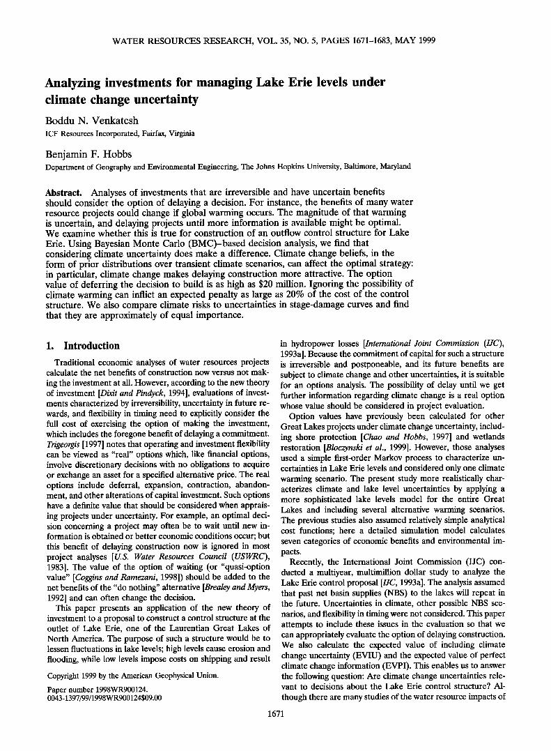
Figure 1. Bayesian Monte Carlo simulation-based two-stage decision tree.

from the Oregon State University, Goddard Institute of Space Studies, and General Fluid Dynamics Laboratory (GFDL) GCMs. After inputting the historical and modified (2 x CO2) temperatures and precipitation in their runoff and routing models, they estimated that mean lake levels could fall between 0.4 and 2.5 m, depending on the lake and the GCM scenario. Mortsch and Quinn [1996] summarize these and other projections of hydrologic impacts in the Great Lakes region.

Such changes could have important economic and environmental impacts. Some of them include reduced hydropower generation, diminished shoreline inundation and erosion costs, water quality deterioration, and fishery changes [Smith and Tirpak, 1990]. As a result, a control structure might provide

fewer flood and erosion control benefits under climate warm-

ing; however, by raising lake levels, its hydropower, navigation, and water quality benefits might increase. Below, we analyze whether considering the possibility of these changes could affect the decision to build such a structure.

3. Modeling Procedures 3.1. Summary of Decision Framework

We pose the investment problem with the option of delay as a two-stage decision process, with 20 years between the decision stages (Figure 1). Venkatesh [1996] also considered trees with additional decision stages along with trees with less than


Table 1. Percentage Change in NBS for the Great Lakes and Three GCMs After 70 Years

ANBS•, %

Lake j MPI GFDL UKMO

Superior -39.6 7.1 16.38 Michigan-Huron -38.4 - 12.6 -28.1 St. Clair -35.9 -8.8 -24.1 Erie -79.8 -40.3 -55.5 Ontario -21.5 -3.9 -3.52

20 years between decision points. The general conclusions concerning the relevance of climate uncertainties and the value of delaying a decision are unchanged by those assumptions.

In stage 1 (year 0) of Figure 1, there are two choices: build a control structure on Lake Erie ("3 Lake"), which would be implemented by year 10, or do nothing and continue regulating just Lakes Ontario and Superior ("2 Lake"). This decision may depend on degree of belief in various climate scenarios, as reflected in prior probabilities. Consistent with the Bayesian philosophy, these priors represent a particular user's degree of belief in the scenarios, which may be based on empirical data, modeling results, or just guesswork; the tree then calculates the implications of those beliefs for the optimal strategy. The model can be easily rerun for alternative assumptions. A range of possible NBS time series are considered by the model through the planning horizon of 80 years. We assume that discounting renders any benefits negligible after that time.

If the decision at time zero is to do nothing, then the decision is revisited after 20 years, which is stage 2 of the process. During the intervening period, NBSs can be observed and inferences drawn as to whether the regional climate is changing. The inference process consists of applying Bayes' law to the prior probabilities, yielding posterior probabilities of the climate scenarios. Upon the basis of those probabilities, either two-lake regulation is continued or a three-lake plan is implemented. The evaluation at that time is based on the expected benefits under a range of possible NBSs over the remaining 60 years.

We consider four climate scenarios in this tree, consisting of one 1 x CO2 scenario (no climate change, which the IJC called the "basis of comparison," or BOC) and three transient scenarios. The latter scenarios are obtained from the Max Planck

Institute (MPI), GFDL, and United Kingdom Meteorological Office (UKMO) GCMs (Intergovernmental Panel on Climate Change (IPCC), Climate change scenarios: Projections for IPCC Working Group II assessment, edited by S. Greco et al., working document, Washington, D.C., 1994) (hereinafter re- ferred to as IPCC, 1994). We assume that the user can quantify their prior (year 0) degree of belief in each scenario by a subjective probability. We also assume that it is appropriate to update these probabilities by Bayes' law, and that the best source of information are the observed NBSs themselves, rather than other climate variables. This is because the im-

mense uncertainties involved in downscaling GCM scenarios to regional climate and hydrological impacts [Leavesley, 1994; Rogers, 1994] mean that even if global climate warming was concluded to be definitely underway, the implications for Lake Erie would still be highly uncertain. However, more general formulations are possible in which several variables can be monitored simultaneously, if their correlations are considered.

The Bayesian model of Bloczynski et al. [1999], for example, includes both NBS and the results of international studies of

climate change in the updating process. Each of the transient GCM outputs consist of a set of dif-

ferences between monthly averages (over a 10-year period) of precipitation and temperature for the eighth decade of simulation and the starting decade. Using the IPCC (1994) procedure and methods described 'in section 3.3, we downscaled the precipitation and temperature changes and estimated NBS values for each of the five lakes' basins. The resulting impact of each of the climate scenarios upon NBS after 70 years is shown in Table 1. We will assume that in intervening years that the expected NBS for each lake changes linearly from year 0 to year 70 under those scenarios.

At the end of each branch of a decision tree is the payoff for a particular combination of a decision and NBS sequence. Here, payoff is annualized net benefit (dollars per year), defined as a weighted sum of economic and environmental objectives. The tree in Figure 1 shows the average value across NBS realizations for a particular decision and climate scenario.

3.2. Bayesian Monte Carlo Analysis

The heart of Bayesian analysis is the use of observations or other information (e.g., expert judgment) # to revise a prior distribution P( 0 ) of a "state of nature" 0 (model parameter or some other uncertain quantity), yielding a posterior distribution P(O/#) [Clemen, 1996]. Bayes' law is used to make that calculation:

P(O/g) = P(g/O)P(O)/P(g)

where

P(g) is the unconditional probability of observing g,

P(g) = •oP(g/O)P(O)

(1)

and P( g/0 ) is the conditional probability of observing g, given state of nature 0. If 0 is a continuous quantity• then an integral is substituted for the summation in (2). In our case, g consists of an observation over the first 20 years of whether the NBSs have been low, medium, or high, while 0 are alternative climate scenarios (no change (BOC), GFDL, MPI, or UKMO). Bayes- ian analysis has previously been widely used to estimate water system parameters. By embedding Bayesian analysis within decision trees such as Figure 1, it can be used to optimize water system control and design [e.g., Davis et al., 1979; Krzysztofow- icz, 1983]. Bayesian analysis has been recommended as a suitable approach for updating beliefs regarding climate change, evaluating water resource development strategies under climate uncertainty [Krzystofowicz, 1994; Hobbs, 1997; Hobbs et al., 1997; M.B. Fiering and P. Rogers, Climate change and water resources planning under uncertainty, draft report, In- stitute for Water Resources, U.S. Army Corps of Engineers, Fort Belvoir, Virginia, 1991], and analyzing climate change prevention strategies [e.g.,Arrow et al., 1996]. However, a practical difficulty in applying Bayesian analysis has been the need for tractable methods to calculate P(g/O) and P(O/g). Often, simplifications are made. For instance, Chao and Hobbs [1997] and Bloczynski et al. [1999] assume that Lake Erie levels (one of their sources of information g) follow a first-order Markov process, given the climate scenario 0. This permitted them to use stochastic dynamic programming (SDP) to determine the optimal timing for shore protection investments and wetland rehabilitation, given uncertainties in lake levels and climate

(2)


change. However, Slivitzky and Mathier [1994] have found that more complex models better represent NBSs for the Great Lakes. For instance, Rassam et al. [1992] model annual NBS for each of the five Great Lakes by a shifting-means process that accounts for both persistence over time and correlations among the lakes. A multivariate annual-monthly model is used to disaggregate annual values for each lake into monthly values. Analytical expressions for P( #/0 ) are not possible in that case, and the state space becomes too large for a SDP (as state variables would be required for each lake, along with an additional set of state variables specifying the probability of each possible mean in the shifting mean model).

Bayesian Monte Carlo (BMC) analysis, first introduced by Hornberger and Spear [1980] and Spear and Hornberger [1980] and further developed by Dilks et al. [1992], offers a practical alternative when complex stochastic process models underlie the P(#/0). The approach is as follows. Simulation is used to quantify P(#/0) by assuming a value of 0 and then making random draws of the other variables and noting the resulting distribution of #. This is repeated for all values or a sample of 0. The outcomes of the simulations can be used directly as the distribution P(#/0) under the assumption that each outcome is equiprobable, as we do below; or an analytical form of P(#/0) can be fit to the results. Then, given actual observations of #, the prior P(0) can be updated numerically by Bayes' law.

Dilks et al. [1992] apply the BMC technique to a model of river dissolved oxygen to determine posterior distributions for nine uncertain parameters, such as reaeration rate. Pat- wardhan and Small [1992] use BMC analysis to evaluate uncertainties associated with the predictions of sea level rise and the role that observed data and research plays in reducing this uncertainty. Brand and Small [1995] present BMC methods for updating uncertainty in the predictions of an integrated environmental health risk assessment model. Dakins et al. [1996] employ BMC analysis to compute how much a sampling pro- gram would reduce uncertainties in PCB concentrations.

Patwardhan and Small [1992] and Dilks et al. [1992] stress that the basic challenge is the development of a likelihood function for the observed model outputs. They also state that the technique's weakness is its computational requirements. Our case study reinforces these points.

We use BMC analysis to compute the posterior probability of climate change by developing a likelihood function for the NBSs for years 1-20 based on Monte Carlo sampling using the model of Rassam et al. [1992]. Then using the prior distribution of the climate scenarios and this likelihood function, we compute the posterior probability of each scenario. Having developed the posterior distribution, we can fold back the decision tree (Figure 1) to compute the Bayes optimal decision. Figure 2 summarizes the steps to be undertaken in this analysis; in the remainder of this section, and in section 4, we describe the methods used in each step and their results. Steps 1 and 2 (section 3.3) generate synthetic NBS series assuming no climate change and then introduce climate warming into these traces. Step 3 (section 3.4) uses the NBS traces generated in steps 1 and 2 to obtain net benefits for each alternative using the CWRU Impact Model. Step 4 (section 3.5) classifies the NBS traces generated in step 3 as low, medium, or high, the categories used to calculate posterior probabilities of the climate scenarios. In step 5 (section 4.1) the probabilities and net benefits developed in steps 3 and 4 are plugged into a decision tree, yielding an optimal strategy, given the user's beliefs and

Step 1. Generate synthetic Basis-of- Comparison NBS (without climate change)

I Step 2. Introduce Climate Change ] trend into synthetic NBS traces

Step 3. Use each NBS trace to drive Hydraulic, Economic, & Environmental models to obtain net benefits of each alternative

I Step 4. Classify NBS traces as Low, Medium or High, I and calculate prior and posterior probabilities

I StepS'Insertbenefitsintøtwøstagedecisiøntreetø I obtain optimal decision strategy and its expected worth

Step 6. ComputeEVPI, EVIU, and option value of waiting

[ Step7. Repeat Steps S,6for a two stage decision ] problem under shoreline damage uncertainty

Figure 2. Flow chart of the analysis.

values. Step 6 uses the tree to compute EVPI, EVIU, and the option value of waiting (sections 4.2-4.4). Finally, in step 7, a similar analysis is undertaken for shoreline damage uncertainties, permitting an assessment of the importance of climate uncertainty compared to another planning uncertainty (section 4.5).

3.3. Net Basin Supply Scenario Generation (Steps 1 and 2)

In the first two steps we generate a sample of monthly NBS for each lake for 90 years under each climate scenario 0. Let NBS0h = {NBSohjt; j = Superior, Michigan-Huron, St. Claire, Erie, Ontario; t = 1, 2, ..., 1080} be the h th (h = 1, 2, ..., No) sample time series of monthly NBS (in cubic meters) under climate scenario 0 (0 = BOC, MPI, GFDL, UKMO). In step 1 the "no climate change" NBSs (NBSBoc•) are generated using the method of Rassam et al. [1992]. In that model random annual NBSs are generated for each lake, accounting for autocorrelations and between-lake correlations; then the annual NBSs are disaggregated to monthly values. The randomness in NBS stems from natural variability in rainfall and evapotranspiration. A variety of distributions are used for each lake and time period, including normal, lognormal, and gamma. The model includes a Markov shifting-mean rep- resentation to account for persistence in the historical record. In our analysis, NBoc = 100 samples of NBS were drawn for that scenario. In the BMC method, each of the samples is assumed to be equiprobable; that is, P(z = NBSBoc•/0 = BOC) = 0.01. An example of a Lake Erie BOC NBS trace is shown as the upper line in Figure 3.

The creation of hydrological scenarios under changed climate conditions (step 2) is controversial and rightfully so. Our procedure is an attempt to be transparent, uncomplicated, and to yield plausible NBSs. Some assumptions of the procedure are as follows:

1. The downscaling procedure for mean temperature and precipitation changes used by Croley [1990] is appropriate.

2. The response of expected annual NBS to the transient


1600

1200

800

NBS 400 mm overlake area

ii! , -400 ,

-800

Year

Erie NBS_IxCO2 --' Erie NBS_MPI ........ Erie NBS_2xCO2

Figure 3. Example of NBS trace generated for Lake Erie under 1 x GO 2 conditions and the corresponding 2 x CO2 and transient traces (MPI downscaling results).

scenarios' changes in mean precipitation and temperature in year 70 are similar in nature to the responses Croley [1990] calculated for three steady state GCM 2 x CO2 scenarios. This assumption may exaggerate the impacts of climate warming upon NBS, since groundwater and soil moisture storage means that there are lags in the hydrologic system's response to climate shifts. That would imply that transient responses are less than the steady state responses Croley [1990] calculated.

3. The mean annual NBS in each year changes linearly between the year 0 mean and the estimated year 70 mean. This assumption is adopted for simplicity and because no particular nonlinear assumption is more plausible.

The resulting method for obtaining NBS0h for 0 = MPI, GFDL, UKMO can be briefly summarized as follows. First, GCM precipitation and temperature scenarios are downscaled to each lake. Second, statistical relationships based on work by Croley [1990] are used to infer the impact of downscaled 2 x CO2 temperature and precipitation changes upon mean annual NBS. Third, 2 x CO 2 NBS traces corresponding to each NBSBo½& (e.g., the dotted line in Figure 3) are generated using statistical relationships between Croley's [1991] 1 x CO2 and 2 x CO2 NBS scenarios. Finally, each transient scenario's NBS in each month over the time horizon (the middle line in Figure 3) is obtained as a convex combination of the generated 1 x CO2 and 2 x CO2 NBS scenarios, with the weight given to the 2 x CO2 scenario increasing linearly over time. These calculations are explained further in the appendix.

3.4. Net Benefit Calculation for Each NBS Realization and

Decision (Step 3)

The next step is to calculate how well each possible decision performs for each NBS sample NBS0h. Let dk designate one particular decision sequence. Thus, in the decision tree of Figure 1, there are three possible sequences: d• = {two-lake regulation all years}; d 2 = {two-lake years 1-30, three-lake regulation chosen in year 20, implemented for years 31-80}; d3 = {three-lake adopted year 0, implemented in year 11}. The purpose of this step is estimate the net benefits attached to

the end points of Figure l's tree. These are the annualized net benefits B(NBSoh, dk) for each NBS sample and decision sequence.

B(NBSoh , d•:) is computed using the CWRU Impact Model. We assume that we are already 10 years into global warming at the time of the study. Thus the first 10 years of simulated NBS are disregarded. Since there are 400 samples and three decision sequences, the impact model was run 1200 times for years 11-90. The cost considered is the expense of implementing the three-lake plan; the benefits are expressed by seven social and environmental indices. These include value of hydropower from Great Lakes and St. Lawrence facilities (dollars per year), erosion and inundation damages estimated from stage-damage curves (dollars per year), avoided shore protection costs (dollars per year), navigation costs based on the effect of levels on loadability of ships (dollars per year; based on the model of Keith .[1989]), wetlands (by lake) (meters of vertical extent between landward upper edge and lakeward lower edges [IJC, 1993c]), and expected oxygenated hypolimnion in the Lake Erie central basin (cubic meters).

To compute annualized values, present worths were first obtained based on an interest rate of 5% and then multiplied by the appropriate capital recovery factor. Annualized capital and operation and maintenance costs are then subtracted to yield net annualized benefits. The assumed 5% real rate is close to the 8 5/8% nominal rate used for water planning by the federal government at the time of analysis, given an inflation rate of 3%. The effects of alternative rates (2% and 10%) were examined by Venkatesh [1996]; the lower rate had the predict- able effect of increasing the maximum investment that could be justified, and the higher rate had the reverse effect. Trigeor- g/s [1996] notes that traditional decision tree analyses similar to the one we use in this paper generally use a single risk-adjusted discount rate. Using such a rate can distort decisions since asymmetric claims on an asset do not have the same riskiness as the underlying asset itself. This is because the flexibility embedded in future decision nodes changes the payoff struc-


ture and risk characteristics of an actively managed asset and thus invalidate the use of a constant discount rate. Neverthe-

less, we use a constant real discount rate in this analysis because large government water projects do not have a complete market for risk (i.e., complete hedging opportunities do not exist) and thus it is operationally difficult to compute such a rate. Furthermore, the federal government itself computes net benefits of projects using a single discount rate.

An additive value function with linear single attribute value functions is used to combine the economic and environmental

benefits into a single benefits index [Chankong and Haimes, 1983]. We chose not to include risk attitudes via nonlinear functions [Keeney and Raiffa, 1993] for four reasons. First, the linear model is simple. Second, there is evidence that water planners have more confidence in additive value functions than more complex approaches [Hobbs et al., 1992]. Third, Hobbs et al. [1992] and others have found that changes in weights usu- ally affects decisions more than risk attitudes in multiattribute analyses. This result was confirmed here; when risk averse (convex) utility functions are used instead of linear functions, the decisions are unchanged unless the functions are highly nonlinear. Fourth, the U.S. government is officially risk neutral in planning •tudies [USWRC, 1983].

The weights for the value function were chosen by 16 Great Lakes managers using a direct rating procedure [Chao et al., 1999]. The weights converted each impact into dollars. The weights assigned to the various economic impacts often differed from each other because of intangibles or credibility problems associated with some of those impacts.

3.5. Calculation of Probabilities for Tree (Step 4)

The first step in developing the probability distributions in Figure 1 involves classifying NBS traces (generated using the above convex combination procedure) for years 1-20 as either # = "low," # = "medium," or # = "high." The high NBS category includes NBS traces where there is clearly no decreasing trend. The low NBS category includes NBS traces which follow a distinctly declining trend. An intermediate category includes more ambiguous NBS. We decided to divide the NBS traces into only three categories instead of four or more in order to ensure sufficient sample sizes in each category. Addi- tional categories would require more computational effort.

The classification of NBS could be based on average NBS over that period, but that would overweight early NBS (when climate change should not be reflected much in the NBS) and underweight later NBS (when climate change should most clearly manifest itself). Instead, we used a simplistic Bayesian method to classify the traces based on whether a decreasing trend is detected [Venkatesh, 1996]. This simple procedure differs from the Bayesian procedure used to update the probabilities in Figure l's tree; the latter is explained below.

Below, we develop the various probability distributions shown in Figure 1. Let P( 0 ) equal prior probability of climate scenario 0; P(CC) equal prior probability of climate change, E0=MPI, GFDL, UK1VIO P(0); and No,g equal number of NBS traces from scenario 0 classified as class g. Here, Eg No,g = 100, the total number of NBS samples for each scenario. Using the above notation, we can compute the decision tree probabilities as follows. The conditional probability of observing g, given a scenario 0, is No,g/100, assuming that samples are equiprobable. Then Bayes' law (1) can be used to obtain the posterior probability of each scenario P(O/g).

For instance, in Figure 1 we assume that P(BOC) = 1/2 and

P(MPI) = P(GFDL) = P(UKMO) = 1/6. We chose these probabilities on the basis of results from our workshops [Chao et al., 1999]. Our 50:50 priors reflect the considerable disagree- ment that was present among the workshop participants concerning the likelihood of significant global warming. The equal probabilities given to the three GCM scenarios of climate change are justified by Laplace's rule: If there is no information that justifies differentiated probabilities, assume equal likelihood. In an actual application, each user would carefully elicit prior probabilities for each scenario, undertake the analysis, and then perform sensitivity analyses. The decision ana- lytic framework that we have developed permits convenient exploration of the implications of different people's beliefs.

Continuing with the example, the classification of NBS re- sulted in 17% of the 100 BOC traces being labeled as "low" (i.e., P(low/BOC) = 0.17), as were 76% of the MPI traces, 29% of the GFDL traces, and 46% of the UKMO traces. Using (2) to combine this information with the prior probabilities allows calculation of P(low), the overall probability of observing•a low NBS; the result is 0.34. Finally, Bayes' law gives the posterior probabilities, given g = low. For instance, P(BOC/ low) = 0.25, indicating that observation of diminished NBSs implies that the likelihood of no climate change is less than thought initially (P(BOC/low) < P(BOC) = 0.5).

4. Decision Analysis Application We now guide the reader through single- and two-stage

decision analyses (steps 5-7). The data assumptions are summarized in Table 2. A critical assumption is the investment cost of three-lake regulation, $375 million. This is actually well below the projections of the IJC, which exceeded $1 billion, including shore protection works along the St. Lawrence River to prevent damages from more variable flows. Such costs were well in excess of conceivable benefits of the project, and, the IJC rejected the plan. However, for the purpose of this article, which is to illustrate the calculation of option values and how climate uncertainties could matter in a decision, we use a lower cost in order to make the decision more interesting. We note that some managers have argued that smaller control structures that were not fully considered by IJC [1993a] have more favorable economics [Chao et al., 1999]; consequently, our conclusions concerning the importance of climate change might be relevant to analyses of those options.

4.1. Strategy Optimization (Step 5)

We discuss here the effects of climate change uncertainty on decisions and net benefits under single- and two-stage analysis under the assumptions defined in Table 2. In a single-stage case the decision made in year 0 is once and for all. In the two-stage case (Figure 1) we can revisit the decision after 20 years in case the strategy to wait is chosen at t = 0. The difference in the expected benefits of the two cases is used to quantify the quasi-option value of waiting. •

4.1.1. Single-stage analysis. In a single-stage problem we would either build the structure now or never. In this analysis we see several trends. First, the MPI scenario's net benefits are lower than others because it is the most extreme warming scenario. Its NBS scenarios are the lowest, causing losses of hydropower and increases in navigation costs. Second, three- lake regulation is slightly more beneficial under BOC (no climate change) and more so under the MPI scenario (which, as Table 1 indicates, represents extreme climate change). But


Table 2. Base Case Assumptions

Problem Attribute Assumption

Number of stages considered in analysis Uncertainties Value of information indices

Three-lake plan Number of NBS traces

Prior probability of climate change Prior probability of a particular GCM-

based climate change scenario Stage length Time for construction of structure Interest rate

Payoff Investment cost

O and M cost

single and two stages considered separately climate change, net basin supply EVPI and EVIU

50,000 feet3/s * 100 each of BOC, MPI, GFDL, and UKMO P(CC) = 1/2 P(MPI) = P(GFDL)= P(UKMO)= 1/6

20 years for two-stage case 10 years 5% (real) annualized net benefits in $M 3755M 3.1$M/yr

*Fourteen hundred cubic meters per second.

under the moderate climate change scenarios (GFDL, UKMO), two-lake is preferred. This seemingly odd nonmono- tonicity occurs because under the intermediate scenarios, lake levels drop enough to moderate the shoreline damages that occur under BOC but not so much as to incur the large navigation costs that are inflicted by MPI.

On folding back the single stage decision tree (shown by Venkatesh [1996]), the optimal strategy is not to build a structure on Lake Erie. The optimal expected annual worth of net benefits is 878.9 million dollars per year ($M/yr). The investment cost for three-lake regulation that would result in a tie between three-lake and two-lake regulation is 322 $M under a 50:50 prior for climate change. We also calculate this break- even cost for other prior probabilities. The dotted line in Fig- ure 4 shows that as the chance of climate change increases, the one-stage break-even investment cost decreases. The area below the dotted line represents the build-now decision, while that above represents the choice to never build. This result occurs because moderate climate warming (the GFDL and UKMO scenarios) would give some of the same shore protection benefits that three-lake regulation would provide. The decision is therefore sensitive to the decision maker's prior probability of climate change, that is, climate uncertainty matters.

Two-lake regulation's expected benefit exceeds three-lake regulation's by only 878.87 - 876.76 - 2.11 $M/yr. This difference may seem insignificant because the overall magnitude of benefits is so high. However, the bulk of those benefits are $1.2 billion per year of hydropower sales; implementation of three-lake regulation affects them by just a fraction of 1%. In contrast, the flooding and erosion costs that the public are so concerned about are on the order of 40-80 $M/yr; three-lake regulation cuts them by 14% under BOC, while global warming can cause as large as a 45% decrease. From this perspective the differences between alternatives are important.

As a sensitivity analysis, the prior probabilities in the above single stage analysis can be easily manipulated. For instance, let us assume that P(MPI) = P(BOC) = 1/2 and P(GFDL) = P(UKMO) = 0. In that case, three-lake regulation instead has an annual benefit 4.9 $M greater than two-lake regulation, mainly because of the navigation benefits of maintaining higher lake levels.

4.1.2. Two-stage analysis. This analysis includes the additional option of waiting 20 years (Figure 1, Table 2). At the end points of Figure 1, rather than showing B(NBSoh , dk) for each trace (which would result in the display of 1200 values),

we show the expectation Zh6g (1/No,a)B(NBSoh, dk) for each of the far right chance nodes. If the decision is postponed, then we can use the additional information acquired during our wait (20 years of NBS data) to update our prior probability of climate change. As explained in section 3, Bayes' law is used to compute the posteriors, which involves classifying the 400 NBS traces into three groups (low, medium, and high), as shown in the figure.

The optimal two-stage strategy is found by folding back Figure l's tree. The solution is to wait at t = 0 and implement three-lake regulation only if NBSs decline enough to indicate that lake levels are likely to drop because of climate change (# = low). In that case P(BOC/#) falls to 0.25 (compared to its 0.5 prior), and the likelihood P(MPI/#) of the high- navigation cost MPI scenario has climbed to 0.38 (from its 0.167 prior). This model appears to justify Lake Erie regulation in order to raise lake levels and decrease navigation ex- penses. The optimal annual benefits under waiting is 879.90 $M/yr, which is 3.2 $M/yr more than building immediately.

Analogous to the single-stage analysis, we have computed investment break-even thresholds for which the "to build" de-

cision changes "to wait," and then further "to never build" for a range of prior probabilities of climate change. To ease comparison with the single stage results, Figure 4 shows the investment break-even threshold for the two-stage case as continuous lines. The figure reveals that under most values of the probability of climate change P(CC), adding the option of

Capital Cost (US)

•i wait under 2 stage, build now under I stage wait under 2 stage, never build under I stage lOOO

750 1 Never Build ß

500

250

0

0 0.2 0.4 0.6 0.8 1

Prior P(Climate Change)

Figure 4. Decisions in year 0 as a function of investment cost and probability of climate change under single- and two-stage analysis.


EVPl(M$)lyrl :::i:.•111 •!i :'::"•"':'•" ':•'::i (•;/•:"'•:'½•':!•: '•:•-'.•.m•.*.•:•'.-'•'.--•..m•' ::::-::.:.::•-:.--' .,:½•ig!!!':': '"•'"'"'":•:•:•'•':i'"'"':.' '•:" '"":"'"'"'""""•-----:•'-'":..•j•{ ..,.•:?#½i.-,.";-.-':,"•:' '-";-:,'.:-':-'-'--'";-:'-"--'--'•:•' .:'+"" ""'•,' •or P(CC) : -•:i;;ii.;" "';"":i:::•';""•:';• :"x•'""•g'a::-"'"<' ß :..?-'.-'.•!

-,- .i::::i :'.i•:: '* .:: .{."'.'" •.: ' 1 :.½:: ,i..' -:;, .';'::'= ';.'•- '"' ,=.,,*! ..... *; ;-'•½- ........ ';':' , i"' •.'::'"' ::::::::::::::::::::::::::::::::::: .•*:},'.' •;::i;" 0 0 *:;;::: ......... '?::.:. ........ •*.* ................... ?.-*- ................. ;-5..- .................... ;i•;'.::.:.:...:...::.:..;½';,i.::...:.......;.:.:•';:• ................... 125 200 275 350 425

Investment Cost (MS)

Figure 5. Sensitivity of EVPI with respect to probability of climate change and investment cost.

delay reduces the investment break-even cost for immediate construction, while increasing the break-even level for never building. The region between yields a "wait" decision. Part a of that region corresponds to investment cost and probability values for which waiting (under the two stage analysis) is substituted for building immediately (in the one stage case), while part b represents values where there is now a positive probability of building later instead of never building. The graph shows that the break-even thresholds, and hence the decisions, significantly depend on the user's belief in climate change. This implies that for costs in that range, climate change should be explicitly considered by planners.

4.2. Expected Value of Perfect Climate Information (Step 6)

EVPI is the difference between the expected payoff given that the decision makers know before choosing whether climate change will occur and the expected payoff given that they perform no experimentation [Clemen, 1996; Smith, 1992]. Al- though perfect information is impossible, EVPI gives an upper bound to the value of imperfect information for the problem and may therefore allow some research to be ruled out on cost grounds alone.

We now calculate the value of perfect information with respect to whether or not climate change is occurring. To ease its calculation, we construct a decision tree that shows that we know whether or not the climate is changing before a decision needs to be made. However, before choosing, we do not have any further information on which climate change scenario 0 will happen, or what the NBSs will be. The expected net benefits under perfect information concerning whether or not BOC will occur are 879.37 $M/yr. EVPI is computed by sub- tracting the expected net benefits of the prior (single stage) analysis (878.87 $M/yr) from the expected value under perfect information (879.37 $M/yr). EVPI is therefore 0.50 $M/yr, for a present worth (PW) of 9.9 $M (at 5%/yr interest). If instead perfect information is assumed for which specific climate scenario 0 is occurring, EVPI grows to 1.97 $M/yr (38 $M PW). Compared with the investment of $375 M, these values may

appear low; but compared to the 2-3 $M/yr differences among alternatives in the one- or two-stage analysis, they are significant.

EVPI is sensitive to both the prior probability of climate change and investment cost. Figure 5 shows that at a low investment cost, EVPI is zero because the decision is to build whether or not climate change is believed to be likely. At a high investment cost EVPI is again zero because the decision not to build is made irrespective of climate change beliefs. Between these extremes, perfect information about climate change can make a difference in decisions, and therefore EVPI is positive.

Now we turn to the effect of belief in climate change. When the prior probability of climate change is 0 or 1, EVPI is zero as perfect information, by definition, contributes no new information. The maximum EVPI of 1.5 $M/yr (PW of 29 $M, about 10% of the investment) occurs at P(CC) = 0.5.

4.3. Expected Value of Including Climate Change Uncertainty (Step 6)

EVIU equals the difference between the expected benefits of (1) a decision based on a probabilistic decision analysis and (2) a decision that ignores uncertainty but is evaluated under the probability distributions used in the decision analysis [Mor- gan et al., 1990]. Thus EVIU is the expected value of the extra information obtained by incorporating uncertainty in the decision process; for a rational decision maker it is nonnegative. A mathematical definition for the single stage problem is as follows [Morgan et al., 1990]. Let 0• be the value of state of nature i assumed in the decision process when ignoring uncertainty. For continuous 0, this might be taken as E(0); here, however, we assume it is 0• = BOC. Note that if instead Oi• is assumed to be, say, MPI, a different EVIU results. Let d i• be the optimum decision when ignoring uncertainty:

d ½u = {mlNeB(0iu , d)}-' (3)

where { }-z is the decision strategy that solves the problem within the brackets. Then


...... '•< x- ................. •::-' ,,,•, vo ..*. ........... •:", .... i:.:•. • .-".' :::::::•*:;> • .......... ,•.:•

..... .. • . U.• 8 • ' ..... • ••/••/ ' PriorP(CC) ' . ..... .:•:•'•:• ...... '• --•,:--:.•4•..::m•.:.•.-":•. ,•/• ...... . ........ 0 4

4 0.2

ß , '•':-' '• ' '• • .,'I,• " 0

•00 200 •00 400 $00 •00 700

Investment Cost (•$)

Figure 6. Expected value of including climate change uncertain• as a function of investment cost and the probabili• of climate change.

gvIu --- E[B ( O, d • ) ] - E[B (0, d iu) ] (4)

where d* equals {MINdE[B(0, d)]}- •, the optimal decision under uncertainty. We can extend this definition to multistage problems by defining d as a set of contingent actions.

If the prior probability of climate change P(CC) is naively assumed to be zero, then the optimal decision d iu in either the single or two stage tree is to implement three-lake regulation immediately. (Note that to make this calculation for the two stage analysis, the P(#) in Figure 1 would have to be recalcu- lated.) An annualized worth of 884.50 $M would then be (in- correctly) anticipated. However, upon implementing d in in Figure 1, but assuming P(CC) = 0.5, the expected annual worth of net benefits of d iu is correctly calculated as 876.76 $M. In contrast, the optimal strategy d* under P(CC) - 0.5 in Figure 1 is to wait at time 0; the resulting optimal annual benefits is 879.90 $M. Thus under this scenario, EVIU is 3.14 $M/yr (879.90-876.76). Its present worth is 61.5 $M, compared to the investment cost of 375 $M. Hence in this case the value of including climate uncertainty is significant.

Figure 6 displays the sensitivity of EVIU with respect to investment cost and P(CC). We note under the lowest or highest investment costs, EVIU is zero, as the decision d iu obtained when ignoring climate uncertainty is the same as the d* from the BMC-based decision analysis. But for costs between these extreme values, decisions change and EVIU can be positive. EVIU can be as high as 8.8 $M/yr; the PW of that value, 173 $M, is almost half the investment cost. Note also that EVIU grows as P(CC) increases. This is because at P(CC) - 0, the naive assumption of no climate change is actually the true situation, so EVIU is zero. The steepness of the curve with respect to P(CC) in Figure 6 indicates that if a user believes that climate change has a significant probability, ignoring that possibility can be costly.

4.4. Option Value of Waiting (Step 6)

Traditional project analyses assume that the project must be built now or never, ignoring the possibility of waiting until more information or more favorable conditions are obtained.

But rejecting a project keeps the door open for reconsidering it later (as, indeed, the IJC has done more than once with Lake Erie regulation in recent decades). This lost quasi-option value

or opportunity cost should be added to the value of the "do nothing" option. As a result, the decision may change.

In our example we can compute the worth of the real option of waiting by comparing the optimal net benefits of the single- stage problem (section 4.1.1) with those of the two-stage problem (section 4.1.2). Thus the value of the option of waiting for 20 years and then making a decision is 1.03 $M/yr (879.90- 878.87), which has a PW of 20.1 $M. This option value would grow if additional decision stages are included, as shown by the three-stage analysis by Venkatesh [1996].

4.5. Comparison with Shoreline Damage Uncertainty (Step 7)

Climate change is not the only uncertainty water planners must deal with. For protection of the Presque Isle, Pennsylva- nia, beach along Lake Erie, Chao and Hobbs [1997] found that climate uncertainties had less influence on the decision than

interest rate and investment cost uncertainties but more influ-

ence than uncertainties in the rate of climate change, construction period length, or escalation of sand nourishment costs. (For an early study of the importance of a variety of uncertainties in water planning, see work by James et al. [1969].) A major (and controversial) uncertainty in the IJC studies of Lake Erie regulation concerns the stage damage curves used to determine shore and flooding damages. Reduction of those damages would be the largest source of regulation benefits in Lake Erie, yet the methods and data used to derive the curves have been criticized [e.g., Yoe, 1992]. We therefore perform an EVPI, EVIU, and option value analysis for shoreline uncertainties; the magnitude of those values compared to those obtained above for climate help us judge the significance of climate uncertainty. In future work, additional comparisons could also be made with other sources of uncertainty, including political and economic ones (as done by Chao and Hobbs [1997]).

We assume that damage uncertainties at year 0 are such that there is a 1/3 chance that stage-damage curves will be 50% lower than their expected value, a 1/3 probability that they will equal their expected value, and a 1/3 chance of the damages being 50% greater than expected. We further assume that if the IJC waits 20 years before making a decision concerning lake regulation, all uncertainty would be erased (i.e., the decision could be made under perfect information). We set up the


decision trees required for the EVPI, EVIU, and option value analyses, analogous to those for the climate uncertainties. Cli- mate uncertainties were excluded from the trees by assuming e(•OC) = •.

The resulting EVPI, EVIU, and option value under stage damage uncertainty are 5.09, 2.22, and 2.22 $M/yr respectively. The analogous figures for climate change uncertainty, calculated above, are 0.50, 3.14, and 1.03 $M/yr. Thus the results are ambiguous. Although the cost of ignoring uncertainty is larger for climate change than for shoreline damage, EVPI and option value are smaller. We therefore conclude that the two

uncertainties are of roughly equal importance, implying that climate change is as deserving of attention as other uncertainties.

5. Conclusions

Bayesian Monte Carlo simulation-based decision analysis is a practical methodology for computing an optimal strategy for the Great Lakes levels management problem under climate change uncertainty. An important benefit of the approach is that it permits use of sophisticated models of stochastic hydrology and multiple economic and environmental impacts. The method has been used to quantify the option value of waiting for better information on climate, value of perfect information, and the value of explicitly including climate uncertainty. We have found that climate uncertainties can alter water decisions being made now and that climate uncertainties can be as important as other uncertainties. These results are broadly consistent with those of Chao and Hobbs [1997], who found that climate beliefs mattered in a Lake Erie shore protection decision, and those of Fisher and Rubio [1997], who concluded that greater climate uncertainty increases optimal reservoir size.

However, climate uncertainty is not always important. For instance, Bloczynski et al. [1999] and Rogers [1997] found that for coastal wetlands restoration and for sizing and timing of water supply additions, respectively, climate uncertainties did not influence present choices. This is also true for the three- lake regulation option considered by IJC [1993a], whose cost was so large that the proposal was uneconomic even under the most optimistic conditions. Therefore no blanket statement can be made about the relevance of climate change to today's water management problems. Hobbs et al. [1997] proposed a screening procedure designed to identify whether climate change might be important in water planning and for choosing an appropriate method to include climate uncertainties, if significant. If climate change is potentially relevant, then a framework similar to this paper's can be used to quantify manager and stakeholder values along with their beliefs concerning the likelihood and magnitude of climate change, and then show the potential implications of those judgments for the optimal strategy.

Appendix: NBS Generation Under Alternative Climate Scenarios

In this appendix we detail the method outlined in section 3.3 for generating a sample of monthly NBS, NBSoh (see work by Venkatesh [1996] for details). The procedure is summarized in the following four steps.

A1. Precipitation/Temperature Downscaling

For each 0, obtain the mean change in annual precipitation APoj,7 o and annual average temperature A Toj,7 o for each lake

j's basin for the year 70 by downscaling the GCM results for that year by the procedure of IPCC [1994]. For instance, for Lake Erie, the downscaled MPI results are APoj,7o = -3,25% and AToj,7 o = +3.55øC.

A2. Effect Upon Expected NBS

For three GCM models, Croley [1990] shows values of annual Apj (in percent of annual precipitation) and A Tj (in degrees celsius) and the resulting percentage change in mean NBS, A%NBSj, for each lake j obtained using a set of watershed models for the Great Lakes. For each lake j, we fit the following linear relationship to those results:

A % NBS• = 13v•AP• + [3VA rj (A1)

The R 2 were over 0.9 in every case other than the smallest lake, St. Clair. As an example, for Lake Erie,/3vj is 2.04 %/% and /3:r• is -19.7%/øC. We then inserted the previously calculated APoj,? o and AToj,? o in (3) to project A%E(NBSoj,?o), the percent change in expected NBS for that lake in the year 70 under scenario t9. For instance, the downscaled MPI results just given, when inserted in (A1), result in an 80% decrease in NBS, most of which is due to the temperature increase. In contrast, the less severe GFDL results yield only half as much of a decrease. Assuming a linear trend in mean NBS, the expected change in NBS A%E(NBSojt) for years between 0 and 70 can be calculated as

A%E(NBSoit) = (t/840)A%E(NBSoi,7o), V j, t (A2)

0 = MPI, GFDL, UKMO

with t measured in months. This presumes that A %E (NBSoj,o) = 0; that is, in month 0 there has been no departure from the historical mean. The implication of (A2) for the MPI scenario is that expected annual NBS would decrease by about 1%/yr.

A3. Generate 2 x CO2 Sample NBS Traces

A straightforward way of obtaining 2 x CO 2 hydrological scenarios is to take a historical sequence of precipitation and temperature, modify that sequence according to the projected changes in average annual precipitation and temperature, and then run the modified sequence through a runoff model. This sensible approach was taken by Croley [1990, 1991] for NBS in the Great Lakes. Rogers and Harshadeep [1994] observed that such predictions of NBS under 2 x CO2 conditions can often be accurately represented as simple linear functions of NBS under 1 x CO2 conditions. We found that was true for NBS simulations based on the Canadian Climate Centre (CCC) GCM 2 x CO2 scenarios and the methods of Croley [1990]. Croley [1991] reported historical NBS for the five Great Lakes and simulated 2 x CO2 NBS for the same period obtained by adjusting the daily temperature and precipitation records by the annual mean Apj and A Tj from the CCC GCM. From his historical and corresponding 2 x CO2 data, we fit linear equa- tions of the form

NBS2xco2,/t = aim + big NBSHistorical,j t (A3)

for each month rn = 1, 2, ..., 12 and lake j. R 2 was above 0.9 for nearly all months, confirming the observation by Rogers and Harshadeep [1994]; thus our statistical models are a rea- sonable approximation of Croley's hydrological downscaling process. For example, for June in Lake Erie, ajm = --39.5


mm/month and b•m = 0.72 mm/mm (where NBS is measured in mm/month).

We then inserted our 100 BOC NBS samples NBSBoch in (A.3), obtaining an estimate NBS2xco2, h of the corresponding NBS time series that Would have been obtained under the CCC

scenario assumptions and downscaling procedure used by Croley [1990]. An example of such a NBS series for Lake Erie is shown as the bottom NBS series in Figure 3.

A4. Generation of Transient NBS

NBS traces NBS0h for the climate change transient scenarios 0 were then obtained as a convex combination of the BOC and

estimated 2 x CO2 samples, NBSBoch and NBS2x½% h for each sample h, lake j, and non-BOC scenario 0:

NBSohjt-' Aojt NBS2xco2,hjt + (1 -- Xojt) NBSBochjt, •[ h, j, t

0 = MPI, GFDL, UKMO (A4)

where the weight Xoi t is based on how close a given year's expected NBS E(NBSoit) (based upon the adjustment calculated in (A.2)) is to E(NBS2xco2,•t) relative to E(NBSBoc•t), where .the latter two expectations are calculated by averaging over all the samples:

X Oj t •- A % E ( NBSojt) / A % E ( NBS2xco2,jt)

= A %E(NBSojt)/[(E(NBS2xco2,jt)

- E(NBSBocjt))/E(NBSBocjt)], Vj, t

0 = meI, GFDL, UKMO (A5)

As time t proceeds, X oTt increases (since (A2) implies that A%E(NBSoTt) is increasing in magnitude), and the transient scenario NBS will move away from the BOC NBS and more closely resemble the 2 x CO2 NBS. Fighre 3 illustrates this process' the transient trace is between the 1 x CO2 and 2 x CO2 traces, and approaches the latter over time.

Since 100 samples of NBSBoch were created for the no climate change scenario, the above four-stage procedure yields 100 samples of NBSoh for each transient scenario 0 = MPI, GFDL, UKMO, giving a total of 400 samples. Additional traces would be desirable in order to increase the precision of the expected cost estimates, but the computational intensity of the stochastic NBS model and impact simulation models pre- cluded larger samples in our study. This is a drawback of BMC-based decision analysis, as others have noted [Dilks et al., 1992; Patwardhan and Small, 1992].

Acknowledgments. This work was supported by NSF grant SBR 92-23780 and the U.S. Army Corps of Engineers, Institute of Water Resources, with additional support from USEPA STAR grant R825150. Although the research described in this article has been funded in part by USEPA, it has not been subjected to the agency's required peer and policy review and therefore does not necessarily reflect the views of the agency, and no official endorsement should be inferred. We thank W. T. Bogart, J. F. Koonce, and P. T. Chao for their collaboration and the workshop participants for their contribu- tions. We also gratefully acknowledge the many helpful comments by the referees and Editors.

References

Arrow, K. J., et al., Decision-making frameworks for addressing climate change, in Climate Change 1995, Contribution of Working Group III to the Second Assessment Report of the Intergovernmental

Panel on Climate Change, edited by J.P. Bruce et al., Cambridge Univ. Press, New York, 1996.

Bloczynski, J. A., W. T. Bogart, B. F. Hobbs, and J. F. Koonce, Irreversible investment in wetlands preservation: Making optimal decisions under uncertainty, Environ. Manage., in press, 1999.

Brand, K. P., and M. J. Small, Updating uncertainty in an integrated risk assessment: Conceptual framework and methods, Risk Anal., 15(6), 719-731, 1995.

Brealey, R. A., and S.C. Myers, Principles of Corporate Finance, 4th ed., McGraw Hill, New York, 1992.

Chankong, V., and Y. Y. Haimes, Multiobjective Decision Making: Theory and Methods, North-Holland, New York, 1983.

Chao, P. T., and B. F. Hobbs, Decision analysis of shoreline protection under climate change uncertainty, Water Resour. Res., 33(4), 817- 829, 1997.

Chao, P. T., and A. W. Wood, Water management implications of global warming: The Great Lakes-St. Lawrence River Basin, draft report, Inst. for Water Resour., U.S. Army Corps of Eng., Alexan- dria, Va., 1998.

Chao, P. T., B. F. Hobbs, and B. N. Venkatesh, How should climate uncertainty be included in Great Lakes management?: Results of modeling workshops, J. Am. Water Resour. Assoc., in press, 1999.

Clemen, R. T., Making Hard Decisions, 2nd ed., PWS-Kent, Boston, Mass., 1996.

Coggins, J. S., and C. A. Ramezani, An arbitrage-free approach to quasi-option value, J. Environ. Econ. Manage., 35, 103-125, 1998.

Croley, Ii, T. E., Laurentian Great Lakes double-CO2 climate change: Hydrological Impacts, Clim. Change, 17, 27-47, 1990.

Croley, II, T. E., CCC GCM 2 x CO2 hydrological impacts on the Great Lakes, in IJC Water Levels Reference Study, Task Group, Work. Comm. III, Washington, D.C., 1991.

Dakins, M. E., J. E. Toll, M. J. Small, and K. P. Brand, Risk-based environmental remediation: Bayesian Monte Carlo analysis and the expected value of sample information, Risk Anal., 16(1), 67-79, 1996.

Davis, D. R., L. DUckstein, and R. Krzysztofowicz, The worth of hydrologic data for nonoptimal decision making, Water Resour. Res., 15(6), 1733-1742, 1979.

Dilks, D. W., R. P. Canale, and P. G. Meier, Development of Bayesian Monte Carlo techniques for water quality model uncertainty, Ecol. Model., 62, 149-162, 1992.

Dixit, A. K., and R. S. Pindyck, Investment under Uncertainty, Princeton Univ. Press, Princeton, N.J., 1994.

E1-Shaawari, A. H., Dissolved oxygen concentration in Lake Erie (U.S.A.-Canada), J. Hydrol., 72, 231-243, 1984.

Fisher, A. C., and S. J. Rubio, Adjusting to climate change: Implica- tions of increased variability and asymmetric adjustment costs for investment in water reserves, J. Environ. Econ. Manage., 34, 207-227, 1997.

Grima, A. P. L., Enhancing resilience in Great Lakes water levels management, Int. J. Environ. Stud., 44(1), 97-111, 1993.

Grygier, J. C., and J. R. Stedinger, Condensed disaggregation procedures and conservation corrections for stochastic hydrology, Water Resources Res., 24(10), 1574-1584, 1988.

Grygier, J. C., and J. R. Stedinger, SPIGOT.' A Synthetic Streamflow Generation Software Package, technical description, version 2.6, Cor- nell Univ., Ithaca, N.Y., 1990.

Hartmann, H. C., Climate change impacts on the Laurentian Great Lakes levels, Clim. Change, 17, 49-67, 1990.

Hobbs, B. F., Bayesian methods for analyzing risks from climate change, J. Environ. Manage., 49(1), 53-72, 1997.

Hobbs, B. F., V. Chankong, W. Hamadeh, and E. Z. Stakhiv, Does choice of multicriteria method matter?: An experiment in water resources planning, Water Resour. Res., 28(7), 1767-1779, 1992.

Hobbs, B. F., P. T. Chao, and B. N. Venkatesh, Using decision analysis to include climate change in water resources decision making, Clim. Change, 37(1), 177-202, 1997.

Hornberger, G. M., and R. C. Spear, Eutrophication in Peel Inlet, I, The problem solving behavior and a mathematical model for the phosphorus Scenario, Water Res., 14, 29-42, 1980.

International Joint Commission, Levels Reference Board, Great Lakes-St. Lawrence River Basin, main report, Washington, D.C., 1993a.

International Joint Commission, Levels Reference Board, Great Lakes-St. Lawrence River Basin, annex 3, Washington, D.C., 1993b.


International Joint Commission, Levels Reference Board, Great Lakes-St. Lawrence River Basin, annex 2, Washington, D.C., 1993c.

International St. Lawrence River Board of Control, Regulation of the Lake Ontario--Plan 1958 D, Washington, D.C., July, 1963.

James, I. C., B. T. Bower, and N. C. Matalas, Relative importance of variables in water resources planning, Water Resour. Res., 5(6), 1165- 1173, 1969.

Keeney, R. L., and H. Raiffa, Decisions l•th Multiple Objectives: Pref- erences and Value Tradeoffs, Cambridge Univ. Press, New York, 1993.

Keith, V. F., C. DeAvilla, and R. M. Willis, Effect of climatic change on shipping within Lake Superior and Lake Erie, Engineering Com- puter Optecnomics, EPA-230-05-89-058, Washington, D.C., 1989.

Krzysztofowicz, R., Why should a forecaster and a decision maker use Bayes theorem?, Water Resour. Res., 19(2), 327-336, 1983.

Krzysztofowicz, R., Strategic decisions under nonstationary conditions: A Stopping-control paradigm, in Engineering Risk and Reliability in the Management of Natural Resources under Physical Change with Special Emphasis on Climate Change, edited by E. Parent and L. Duckstein, pp. 359-372, Kluwer, Norwell, Mass., 1994.

Leavesley, G. H., Modeling the effects of climate change on Water Resources--A review, Clim. Change, 28, 159-177, 1994.

Morgan, M. G., M. Henrion, and M. J. Small, Uncertainty: A Guide to Dealing with Uncertainty in Quantitative Risk and Policy Analysis, Cambridge Univ. Press, New York, 1990.

Mortsh, L. D., and F. H. Quinn, Climate scenarios for Great Lakes ecosystem studies, Limnol. Oceanogr., 41(5), 903-911, 1996.

Patwardhan, A., and M. J. Small, Bayesian methods for model uncertainty analysis with applications to future sea level rise, Risk Anal., 12(4), 513-523, 1992.

Rassam, J. C., L. Mathier, L. D. Fagherozzi, R. Ray, B. Bobee, and L. Carballad, Beauharnois-Les Cedres spillway design flood study with a stochastic approach, Hydro Quebec, Montreal, 1992.

Rogers, P., Assessing the socioeconomic consequences of climate change on water resources, Clim. Change, 28, 179-208, 1994.

Rogers, P., Engineering design and uncertainties related to climate change, Clim. Change, 37, 229-242, 1997.

Rogers, P., and N. R. Harshadeep, Water policy and management, in

Great Lakes Climate Change, Research Priorities for Assessing the Impacts of Climate Change on the Great Lakes Basin, edited by C. M. Ryan et al., Great Lakes Environ. Res. Lab., Ann Arbor, Mich. 1994.

Slivitzky, M., and L. Mathier, Climate changes during the 20th century on the Laurentian Great Lakes and their impacts on hydrologic regime, in Engineering Risk and Reliability in the Management of Natural Resources under Physical Change with Special Emphasis on Climate Change, edited by E. Parent and L. Duckstein, pp. 235-252, Kluwer, Norwell, Mass., 1994.

Smith, J. B., and D. J. Tirpak, The Potential Effects of Global Climate Change on the United States, Hemisphere, New York, 1990.

Smith, J. Q., Decision Analysis--A Bayesian Approach, Chapman and Hall, New York, 1992.

Spear, R. C., and G. M. Hornberger, Eutrophication in Peel Inlet, II, Identification of critical uncertainties via generalized sensitivity analysis, Water Res., 14, 43-49, 1980.

Trigeorgis, L., Real Options--Managerial Flexibility and Strategy in Re- source Allocation, MIT Press, Cambridge, Mass., 1997.

U.S. Water Resources Council, Economic and environmental principles and guidelines for water and related land resources implementation studies, U.S. Govt. Print. Off., Washington, D.C., 1983.

Venkatesh, B. N., Analyzing investments under climate change uncertainty: Managing levels of the Great Lakes, Ph.D. thesis, Dep. of Syst., Control, and Ind. Eng., Case West. Reserve Univ., Cleveland, Ohio, 1996.

Yoe, C., A critical review of existing and updated U.S. and Canadian stage-damage curves, Reœ. KW405-2-0191, Environ. Canada, Bur- lington, Ont., 1992.

B. F. Hobbs, Department of Geography and Environmental Engi- neering, The Johns Hopkins University, Baltimore, MD 21218. ([email protected])

B. N. Venkatesh, ICF Resources Inc., 9300 Lee Highway, Fairfax, VA 22031. ([email protected])

(Received August 1, 1997; revised November 30, 1998; accepted December 18, 1998.)

Analyzing Investments for Managing Lake Erie...

Documents

Transcript of Analyzing Investments for Managing Lake Erie...