Analyzing Environmental Kuznets Curves Using a Systems ...

Analyzing Environmental Kuznets Curves Using a Systems Dynamics Approach BY Amreen Ahmad

ADVISOR • Brian Blais _________________________________________________________________________________________ Submitted in partial fulfillment of the requirements for graduation with honors in the Bryant University Honors Program APRIL 2017

Table of Contents

Abstract ..................................................................................................................................... 1

Introduction ............................................................................................................................... 2

Background: .......................................................................................................................... 2

Literature Review: ................................................................................................................. 2

Materials and Methods: ........................................................................................................... 20

Introduction to Methodology: ............................................................................................. 20

Experimental Methodology: ............................................................................................... 22

Parameter Explanation (Using Canada as an Example): ..................................................... 23

Variation in Fits of Models (Using Canada as an Example): ............................................. 29

CO2 Parameters: .................................................................................................................. 33

GDP Parameters: ................................................................................................................. 34

Bayesian Information Criterion: ......................................................................................... 35

The Process in Python: ........................................................................................................ 35

Results and Discussion ............................................................................................................ 36

Visualization of Results- BIC Model Comparison: ............................................................ 36

Countries With Very Strong Evidence of Kuznets Effect: ................................................. 46

Final Conclusion: .................................................................................................................... 52

References ........................................................................................................................... 53

(Analyzing Environmental Kuznets Curves Using a Systems Dynamics Approach) Senior Capstone Project for (Amreen Ahmad)

- 1 -

ABSTRACT

This paper studies the Environmental Kuznets Curve by examining the relationship between CO2

emissions and GDP per capita data for 200 countries worldwide from the time period of 1950-

2015. We use multiple dynamical models - including linear, exponential and feedback models –

to search for and quantify the Kuznets effect, the downward shaped U curve in the time-series of

environmental quantities. Using the Bayesian Information Criterion to perform model

comparison, we determine that there is weak evidence of the Kuznets curve existing in all

countries and slightly stronger evidence for it in the OECD and BRICS countries. We discuss

some of the implications of this result.


- 2 -

INTRODUCTION

Background:

The Kuznets Curve is an economic concept with scientific implications. It is a hypothetical curve

that plots economic degradation against per capita income (see Figure 1). Some substitute

variables for the Y-axis are income inequality, Gini coefficient and pollution, all measures of

some impact on society. The X-axis variables can be per capita income, Gross Domestic Product,

Economic Development etc. which show the development of a particular country. The

hypothesis is that as economic factors of a country (such as GDP) increase, at first there is

significant harm on society and the environment. Then, as the country becomes more developed

and wealthy, the curve shifts downwards as they now have money to spend on rectifying issues

of social inequalities and economic degradation. People start to value environmental preservation

more therefore making more environmentally- conscious decisions. The curve plots the country’s

effect on their surrounding environment as they go from an agriculture-based economy to an

industrialized economy (see Figure 2). For the purpose of this paper, the variables we will be

examining are environmental degradation against GDP Per capita. Specific environmental

pollutants that have been researched/ analyzed before include SO2 emissions, CO2 emissions, NO

emissions, chlorofluorocarbons, etc.

Literature Review:

This relationship was first proposed by Simon Kuznets in 1901.

An example of the Kuznets Curve follows:


- 3 -

Figure 1: Displays a classical Kuznets curve with Per Capita Income on the X-axis and Income Inequality on the Y-axis. The inverted U shaped curve can be observed from this data set.

This is an example of the Environmental Kuznets Curve (EKC):

Figure 2: Displays the Environmental Kuznets Curve which has Per Capita Income on the X-axis and Environmental Degradation on the Y-axis. The inverted U shape can be observed from this data set.


- 4 -

There is much criticism about the existence of the Kuznets Curve. In the case of the

environmental Kuznets curve, one explanation for the turning point is that developed countries

outsource manufacturing and other polluting activities to developing countries. Also, Kuznets

Curves have only been found to be applicable with certain pollutants and in certain situations, it

is not a universal theory (11).

In some cases, researchers have observed an N shaped curve as opposed to the inverted U shape.

This suggests that countries pollute as GDP rises and then subsequently spend more money on

environmental rehabilitation while making an increasing amount of money before starting to

pollute again as income continues to rise. The Kuznets curve is also criticized for lacking

predictive power as it cannot predict what the next stage of economic development will be like

and what repercussions that will have on the environment. While there are large criticisms, there

have been studies on Kuznets Curves that set precedent for this one.

The first model of the environmental degradation Kuznets Curve was examined by Grossman

and Krueger in 1991. They used the North American Free Trade Agreement (NAFTA) as the

region they would study. NAFTA consists of the U.S., Canada and Mexico and allows all

countries within the region to ship goods to participating countries without having to pay import

fees and tariffs. It was believed that when Mexico entered NAFTA, both Canada and the U.S.

would move all of their environmentally polluting practices there. This would allow them to

achieve higher levels of environmental quality while pushing off polluting practices to the least

developed country of the group. Grossman and Krueger believed otherwise; they hypothesized


- 5 -

that the existence of free trade in the region would come with higher incomes across the board as

well as stricter environmental regulations. They used the Global Environmental Monitoring

Systems (GEMS) to find data. GEMS was created by the United Nations and the World Health

Organization to monitor air quality around the world on a monthly/weekly basis. Grossman and

Krueger monitored 42 countries’ SO2 levels, smoke/dark matter levels in 19 countries and 29

countries for suspended particulates. These countries ranged from least developed to developed

nations and they also monitored air quality in suburban, rural and urban locations within the

cities. They held several variables constant such as: identifiable geographic characteristics of

cities, common global time trend in the levels of pollution and location/type of pollution

measurement device. They found statistical evidence for the Kuznets curve as levels of the

pollutants in the air rose up until a GDP between $4000 or $5000 (1985 USD measure) before

decreasing as GDP continued to rise (1). Other subsequent studies found similar results thereby

providing evidence for the Kuznets Curve. What remains a primary issue however is how it is

still not widely applicable.

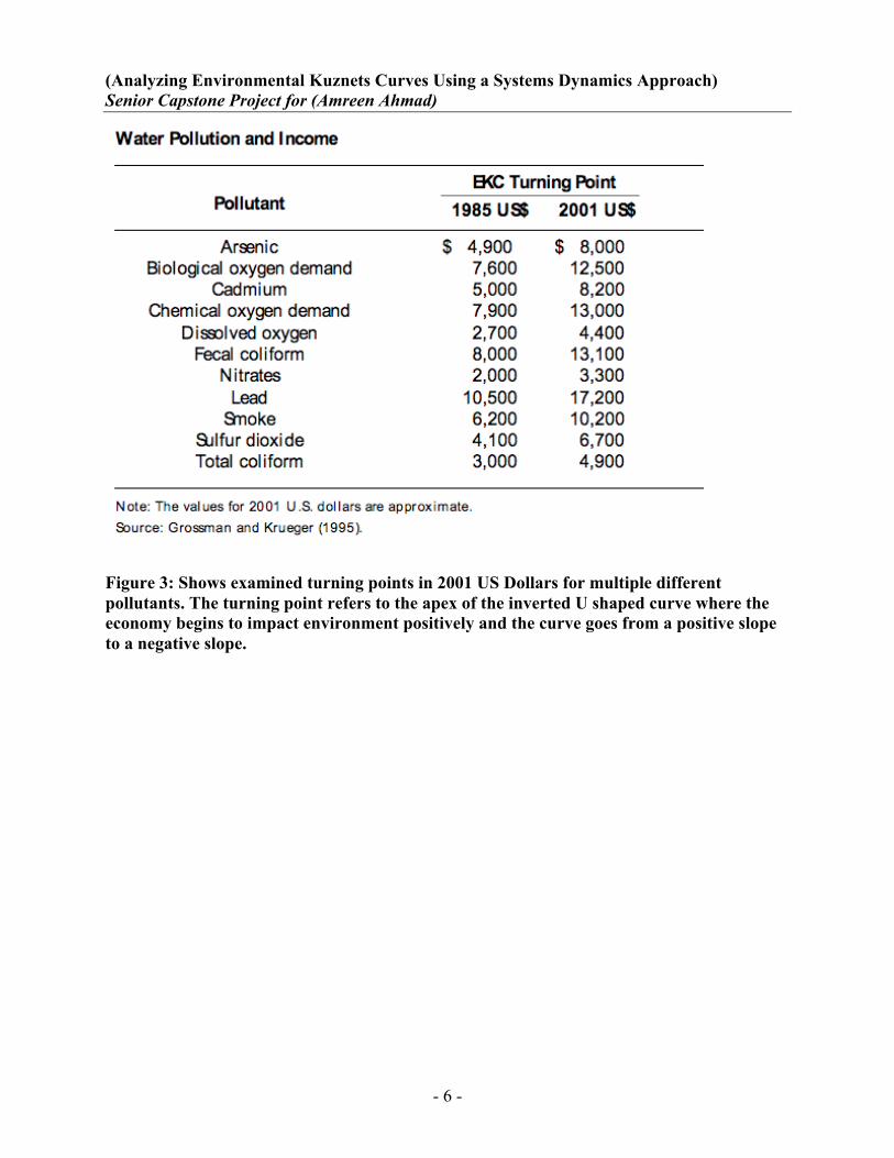
The below charts shows Grossman and Krueger’s estimations of turning points for different

pollutants. The second one is especially relevant as those pollutants have been more widely

studied and well measured, particularly CO2. (2)


- 6 -

Figure 3: Shows examined turning points in 2001 US Dollars for multiple different pollutants. The turning point refers to the apex of the inverted U shaped curve where the economy begins to impact environment positively and the curve goes from a positive slope to a negative slope.


- 7 -

Figure 4: Shows examined turning points in 2001 US Dollars for multiple different pollutants, these pollutants are the more globally recognized and better measured pollutants. One that is especially relevant to this study is the Carbon Dioxide Turning Point.

What we will be looking at in our study is what factors influence the dynamics of pollution and

the economy. We will be using the variables of CO2 emissions and GDP across different

countries to see what other factors may be affecting environmental degradation.

We plan on using Python (computer programming software) to be able to take a dynamical

systems approach to this question. Ranganathan and Swain (3) have used a dynamical approach

that sets the stage for what we would like to do. They looked at the relationship between

Greenhouse Gas Emissions and GDP per capita. One of their first steps was to fit equations for

the rate of change of each specific indicator as a function of the level of the indicator and other


- 8 -

levels of other indicators as well. They then use the best-fit model to predict greenhouse gas

emissions in 2020. They take their research a step further and actually use these predictions to

recommend ways to lower/ maintain emissions. Using the best-fit model they can test what

effects new environmental regulations and income will have on the environment. They found

results indicative of a Kuznets Curve however they list other factors that could explain results as

well. These include: greater environmental awareness, education, and preference for higher

environmental conditions in developed countries. 100 studies published in the past 25 years all

show the following effects:

• Scale effect: when all else is held equal, an increase in output yields a proportionate

increase in pollution

• Composition effect: if sectors with high emission intensities grow faster than sectors with

low emission intensities then subsequent emission will be pushed higher.

• Technical effect: attribute decreasing sector emission intensities to use of more efficient

production and environmentally friendly technologies.

Another previous work we will be relying heavily upon is a paper written collaboratively by

Bryant University Economic Student Jonathan Skaza and Bryant University Professor Brian

Blais about the relationship between economic growth and environmental degradation (10). They

explore models and question the existence of Kuznets curves in this paper. This working paper

examines a few different countries and whether or not the Environmental Kuznets Curve applies

in these diverse countries. We will make parameter comparisons in these cases to attempt to

figure out which conditions yield Kuznets curves and which conditions do not.


- 9 -

As mentioned before, there have been many confounding variables found while conducting

Kuznets Curve research. It is by no means a model that works across different countries with

varying economic development. What has become clear though is that the GDP vs. CO2 emission

data is well measured and well researched giving us a good starting point. This, coupled with a

slew of variables that have been examined throughout other preceding works, should allow us to

use our model to analyze this data further.

An article written by Jean-Thomas Bernard, Michael Gavin, Lynda Khalaf, Marcel Voia (4) is a

good way to start off our study as they use both parametric as well as nonparametric methods.

A small aside, parametric statistics refers to when a statistical test makes assumptions about the

parameters of a population. The parameters can be characteristics that describe the given

population. Data in your study comes from this population. In a non-parametric test, no

assumptions are made about the population.

They also break down their panels regionally, by trends and by temporal instability. They are

working off of literature that proposes that non-linearity of the EKC is not guaranteed. They

broke down countries depending on which ones are in the Organization for Economic

Cooperation and Development (OECD) and which ones are not. A quick note, the OECD is

considered to be a “rich man’s club” as all of the high-income, highly developed countries are

included in it.


- 10 -

OECD Countries BRICS Countries

Australia Austria Belgium Canada Chile Czech Republic Denmark Estonia Finland France Germany Greece Hungary Iceland Ireland Israel Italy Japan Korea Latvia Luxembourg Mexico Netherlands New Zealand Norway Poland Portugal Slovac Republic Slovenia Spain Sweden Switzerland Turkey UK US

Brazil Russia India China South Africa

Table 1: Shows the different countries included in the OECD and BRICS categories.

They were able to discover that the countries in the OECD have confirmed cases of an inverted

U-shape EKC curve whereas others do not. They looked at 114 countries for CO2 and 82 for SO2


- 11 -

from 1960-2007. They grouped countries into 6 groups, one of which contained all of the OECD

countries. When it comes to results, they found that the uncertainties were significant. Their data

shows that the EKC exist in OECD countries and some local-pollutant analyses showed evidence

of EKC’s in other countries. What they determined is that it is difficult to determine an

economically plausible tipping point. The parametric model is the model that they used as the

baseline and they used a nonparametric model as a specification check. The parametric model is

better respected and more valid, this will be the type of model we will use as well. (4)

The next paper that will be discussed is written by Robalino-Lopez and colleagues. They use

systems dynamics to look at the medium term period (1980-2025) of Ecuador to see whether or

not the EKC exists. They use a model that related GDP to productive sectoral structure and

energy mix with the CO2emissions.

The CO2 emissions are studied while quantifying the contributions of 5 factors:

1. global industrial activity

2. industry activity mix

3. sectoral energy intensity

4. sectoral energy mix

5. CO2 emission factors

What is interesting about this study as they are looking at the time period of 1980-2025. This

study gets into the predictive power of the EKC, which we are hoping to delve into as well. They


- 12 -

extrapolate the future trends by using the geometric growth rate. The below figure details the

layers of their model and all of the different variable and factors it includes.

Figure 5: The model used in this study has many subcomponents. This diagram shows the different economic, CO2 energy and intensity as well as energy consumption factors that are included in their model.

They used their model for four different scenarios:

1. Baseline scenario: the GDP, the energy matrix and the productive sectoral structure are

all extrapolated out to 2025 using the geometric growth model.


- 13 -

2. Doubling of the GDP.

3. Doubling of GDP and of the share of renewable energies.

4. Doubling of GDP, doubling of renewable energy share and improvement in the efficiency

of energy use.

The figure below shows the graphed results.

Figure 6: This graph shows the environmental degradation for the different scenarios as well as income elasticity of CO2 and GDP.


- 14 -

This data shows that Ecuador fulfills the EKC hypothesis. The elasticity between CO2 and GDP

leads to two groups. Baseline and Scenario 2 fall into one family whereas Scenarios 3 and 4 fall

into a different family. (5)

We will be relying heavily on the next paper as it is one we will be building our mathematical

model off of. This study is done by Coelho and associates. This paper introduces a framework

that works for both deterministic and stochastic models. This particular study actually focuses on

influenza-like illness rather than the EKC however we are using it because the framework it uses

is highly applicable to our study. This framework is based on the Bayesian Melding Method

which provides an inferential framework that takes into account any and all information related

to a model’s inputs and outputs. In this framework, time-series is a model output.

The extensions that these researchers made to the Melding Method include:

• The ability to use time-series data.

• The use of a multi-chain Markov-chain. This handles non-convex higher dimensional

parameter-spaces.

The Differential Evolution Adaptive Metropolis (DREAM) algorithm was used to sample some

joint posterior probability distributions. DREAM runs multiple adaptive chains at the same with

delayed rejection. In this study they used the simplest model formulation and got results that

corroborate other studies on the same topic. This means that the parameter estimation methods

they used were precise and accurate. The work “proposes a methodological framework to

perform parameter estimation in dynamical models where time series data is available for the


- 15 -

model to be fit against.” There are some limitations of this framework but they can be alleviated

by developing more powerful posterior sampling methods. (6)

The following study is done by Wang and colleagues. This work enhances the connection

between theoretical and empirical analysis while demonstrating the connection between

population growth and the environment. The question they were looking at specifically is how

population growth impacts environmental quality and the EKC. An overlapping generations

(OLG) model is used to deduce the EKC. Within this model, agents live two years and pollution

cannot be avoided. In the OLG there is a trade-off between environmental quality and economic

growth. When they graph their data, the inverted U shape appears. Population growth leads to

more consumption and production, which in turn creates higher levels of environmental

degradation. Under their model, the higher the rate of population growth, the steeper their

observed EKC and the more degradation the environment experiences. Boserup says that

population growth enhances economic development as it forces humans to innovate new

technologies and find ways to make scare factors last longer (7). We are also able to use new

innovations to keep up food production and produce just as much, or even more, with the same

supply of land. According to the Malthusian argument, as our population increases geometrically

and food production increased arithmetically, we will reach a point where we will have no more

arable land, energy and other resources will run out and pollution levels will rise above the

globe’s assimilative capacity. These researchers pooled much data and found that global

population change is positively correlated with increases in CO2 emissions. They also realized

that population change affects emissions much more in developing countries than in developed

countries. The study delved into two facets of environmental degradation including industrial


- 16 -

waste gas emission and industrial solid wastes. Their simulations provide evidence that higher

populations growths lead to a steeper EKC and a higher turning point. Results indicate that the

relationships for industrial waste gas and industrial solid waste exhibits an inverted U-shape like

the EKC. While they did find that when they add population growth into their simulation that the

pollution levels rise, it is at much slower rates within the developed countries. This means that a

population’s growth has a measurable but not very significant effect on pollution levels. (7) The

graphs below show their results:

Figure 7: The graphs above show the EKC that the study generated. They look at both solid waste and waste gas.

The following work to be discussed is written by Farhani and associates. This paper examines

the importance of sustainability related to the EKC. The study looks at two different EKC

specifications for 10 countries (in the Middle East as well as in North Africa) from the time

period of 1990 to 2010. The first specification for EKC that they look at is just a typical EKC


- 17 -

curve plotting income versus environmental degradation. In this data set they find that the

inverted U-shape appears. In the second specification for EKC they examine sustainability

related with human development. In this relationship they observed an inverted U shape as well.

Human development is now considered to be one of the main drivers of economic growth. The

study proposes to replace the income variable of the original EKC with the human development

index (HDI). Another replacement they propose is changing the dependent variable from

emissions to a measure that portrays macroeconomic sustainability such as the Genuine Saving

Index. Panel data methods were used to control for heterogeneity and colinearity among the

variables. The region of Middle East and North African countries was chosen because this

region is believed to have unsustainable economic growth as well as high impact on the

environment, their use of natural resources is unparalleled. The countries they included are

Algeria, Bahrain, Egypt, Iran, Jordan, Morocco, Oman, Saudi Arabia, Syria, and Tunisia. These

are the specifications the used for their two separate EKC models:

1. EKC- CO2 emissions measured in metric tons per capita. Real GDP per capita is

measured in USD Year 2000 levels of inflation. They used a combination of initial level

of life expectancy coupled with secondary education level as their Human Development

Index measure. Normally income is included in HDI but they took it out so as not to

interfere with the other variable which is the GDP per capita.

2. Modified EKC- negative Genuine Savings per capita in USD Year 2000 levels of

inflation. In this specification the HDI includes life expectancy and education like the

first one but also includes income as this time the GDP per capita is not being considered

as a variable. They also include rule of law as an important factor as it affects corruption

in the country when it comes to regulation of environmental issues.


- 18 -

Some other variables that are consistent across both specifications are

• energy consumption, measured in energy use in kg of oil equivalent per capita

• trade openness, measured in % of GDP

• manufacture value added, measured n % of GDP

They hypothesized that there would be an inverted U shaped relationship between CO2 emissions

per capita and per capita real GDP for the regular EKC specifications as well as the same style of

curve for the relationship between negative genuine savings per capita and HDI for the modified

EKC specifications. Both of these were found to be true.

What their EKC model predicts is that:

• as energy consumption per capita increases by 1%, CO2 emissions per capita increases by

about 1.82%

• as trade openness increases by 1%, CO2 emissions per capita increases by about 0.214%

• as manufacture value added increases by 1%, CO2 emissions per capita increases by

about 0.07%

• as Modified HDI increases by 1%, CO2 emissions per capita increases by about 2%

What their modified EKC model predicts is that:

• as energy consumption per capita increases by 1%, negative Genuine Saving (GS) per

capita increases by about 1.153%

• as trade openness increases by 1%, negative GS per capita increases by about 0.252%


- 19 -

• as manufacture value added increases by 1%, negative GS per capita increases by about

0.066%

• as rule of law increases by 1%, negative GS per capita decreases by about 0.019%

What is so impactful about this study is that they use a lot of the data they found to make policy

recommendations to countries. This highlights the significance of the work as this kind of data

and analysis shows how countries are impacting their environments and gives them specific

variables they can focus on to improve. (8)

The following journal article is written by Chow and Li. This paper looks at the persistence of

the use of CO2 when looking at EKC’s because CO2 impacts are indirect, global and long lasting.

Other pollutants such as SO2 and NOx are not as far reaching and long-lasting as CO2 which is

why CO2 tends to be the primary emission that is measured in the literature. This paper mentions

some important limitations of using panel data when estimating parameters.

These include:

• there are econometric problems associated with time series analysis and these crop up

when using panel data as well. What has been determined is that standard regression

analysis simply does not work for time series data

• the primary issue in these models is the existence of unit roots. Therefore, we need to

check the data before we start to discover whether or not there are any unit roots that will

cause issues.


- 20 -

For this analysis they used a t-test on the EKC. They used international data for CO2 emissions

from the International Energy Agency as well as GDP per capita data from the World Bank.

Their data spanned the years of 1992-2004 and looked at 132 countries. They use their t-test on

the EKC treating it as an empirical hypothesis, no theory involved. They did simple t-tests on the

cross-section estimates of the coefficient of the square of log(GDP per capita) in a regression of

log(emission of CO2 per capita). Their results show that the coefficient is negative thus

exhibiting the shape of the proposed EKC. (9)

MATERIALS AND METHODS:

Introduction to Methodology:

The Ranganathan and Swain study (3) used a Bayesian model selection approach to identify the

most accurate model, this is similar to our proposed methodology.

They consider log GDP per capita (G) and total Greenhouse Gas Emissions (E) as their

parameters. They then attempt to find the best-fit models for changes: dG, dE as a function of G

and E (t is the time variable):


- 21 -

In this case G/E is emission efficiency of a country’s economic output and the inverse, E/G is the

emission inefficiency level of the economy. After they set up these functions they make a

polynomial term that captures various linear and nonlinear effects.

They extracted their data from the World Bank. Like Ranganathan and Swain, we will be using

the Bayesian statistical inference approach on dynamical models which will give us best

estimates and uncertainties in parameters and forecasts. Systems dynamics is “a method for

modeling, simulating and analyzing complex systems and its main goal is to understand how a

given system evolves.” (5) This is what we are attempting to achieve.

When you do parameter estimations in nonlinear systems, the best and most widely used

approach is the Bayesian approach. In this case, using uniform priors the Bayesian method is

equivalent to using the maximum likelihood method/ least squares minimization regression.

However if we just did that, we wouldn’t have good estimates for uncertainties. Also in this case,

the methods don’t take into account suboptimal points whereas in the Bayesian methods, they do.

There are two statistical approaches you could take: Bayesian or Frequentist. When you use

uniform priors, they give the same results. When you use informative priors (where we know a

bit more about the parameters, which we do) the Bayesian approach yields superior results. The

Bayesian approach is the superior approach overall. The only time it is not followed is when it is

computationally inconvenient. In that case you can use a frequentist approach as an

approximation.

Mathematical models are used because they combine theory with data to predict empirical

observations. Data is provided in the form of rate parameters and time series and theory in the

form of model formulation. These are combined and provide insight about each other. Parameter

estimation and model selection can allow us to compare competing models and to estimate the


- 22 -

key quantities or parameters that make up these models. As a simple example, a one

dimensional linear model has a slope and an intercept, whereas a quadratic model has an

additional quadratic term. Model comparison techniques tell us which of the two models best

describes the data. Parameter estimation provides the best estimates for the slope, intercept, and

in the case of the quadratic model the strength of the quadratic term. This, combined with data

visualization, can deeply enhance our understanding of the theories. (6)

Experimental Methodology:

1. Bayesian parameter estimation. Based heavily on the model presented in Literature

Review article #6.

2. Data used was CO2 emissions as well as GDP per capita for 200 countries, including

groupings of countries (OECD, BRICS and all countries).

3. Model comparison (if two models fit the same data equivalently then the one that is

simpler is the one that is preferred. Complexity is penalized in these cases.)

4. Found optimal models based on BIC comparison between different models.

5. Searched for evidence of Kuznets curves. This would be a negative quadratic term that

appeared in our data, represented by the b4 term being negative.

6. Possible conclusions include: it could be there, it could be there but masked, it could

not be there, it could be there sometimes (depending on patterns).

The research started off with modeling the data against the original paper in order to see if we

could replicate their results. We were able to use their original formula and data to get similar

results. We then started by updating the data in order to be most current. We have used CO2


- 23 -

metric ton data and GDP per capita (in USD) data per country from 1950 through 2013 in our

research. This data was found on the World Bank website. After creating and modifying the

models in Python we started to analyze each variable in order to answer the following questions:

1. Which terms lead to growth, and why? Do they have to be positive or negative?

2. Which terms lead to decay, and why? Do they have to be positive or negative?

3. In the places where G grows, which terms in the E equation could possibly lead

to the Kuznets effects (increase followed by decrease) and why?

Parameter Explanation (Using Canada as an Example):

In order to better model the EKC and determine the bounds of each parameter, we will look

at an ideal example of the EKC, Canada. From this data we are able to determine the

parameters using the Markov Chain Monte Carlo Method (MCMC).

We started off with loading in the data, seen below in Figures 8 and 9.


- 24 -

Figure 8: Plot of Canada GDP Data.

Figure 9: Plot of Canada CO2 Data.

Then we created different types of models we would use:

Linear:

G’ = a0

E’ = b0

Exponential:

G’ = a0 + a1*G

E’ = b0 + b1*E


- 25 -

Feedback:

G’ = a0 + a4*E*G

E’ = b0 + b4*E*G

From there we looked at each individual parameter to see what would fit best within the

models.

The b0 parameter is one of the first ones we look at. Figure 10 shows that it is very clearly

positive with most of the distribution lying in the positive side. This is the slope of the E

line, the CO2 emissions data.

Figure 10: The graph shows the parameter distribution for b0.


- 26 -

B1 is another parameter with a negative value and small distribution. Figure 11 shows the

distribution.


B4 is one of the most important parameters we are looking at. It is responsible for the

downturn in the EKC which is what we are looking for. The entire range of values for B4 is

negative, shown in Figure 12, which it would need to be in order for the shape of the curve

to turn downwards after it hits the peak. The negative value demonstrated in the case of the

data shows exactly that.


- 27 -


A0 is a growth factor that very clearly has its whole distribution in the positive range, shown

in Figure 13. This accounts for the upwards trend present at the beginning of the EKC and

therefore must be positive to maintain the positive growth. This is the slope of the G line,

the GDP per capita data.

Figure 13: The graph shows the parameter distribution for a0.


- 28 -

A4 is the GDP feedback term and is also negative. Demonstrated by Figure 14.

Figure 14: The graph shows the parameter distribution for a4.

The following distributions, Figures 15 and 16, show the initial value for the GDP and CO2

parameters.

Figure 15: The graph shows the posterior probability distribution for the initial value of G, the variable corresponding to the log of the GDP. Here the best fit value is around G=6.6 a the peak of the distribution, and the range is approximately from G=5.5 up to G=8.


- 29 -

Figure 16: The graph shows the posterior probability distribution for the initial value of E, the variable corresponding to the CO2 emission data. Here the best fit value is around E=5.6 a the peak of the distribution, and the range is approximately from E=0 up to E=35.

Variation in Fits of Models (Using Canada as an Example): After doing the MCMC for each specific parameter we also looked at these graphs that show the

distribution of the lines of “best fit”. The darker the green line, that means there is more overlap

in the best fit line and that is a stronger model.

Starting off with the linear model, we see this figure:


- 30 -

Figure 17: This figure shows the linear E model overlaid on top of the CO2 data as well as the linear G model overlaid over the log GDP data. It is very clear that given the striations in the green line that this is not a good fit for the CO2 data but is a good fit for log GDP since the green line is very dark and has strong overlap. For the CO2 model you can tell it also does not follow the trend of the data.


- 31 -

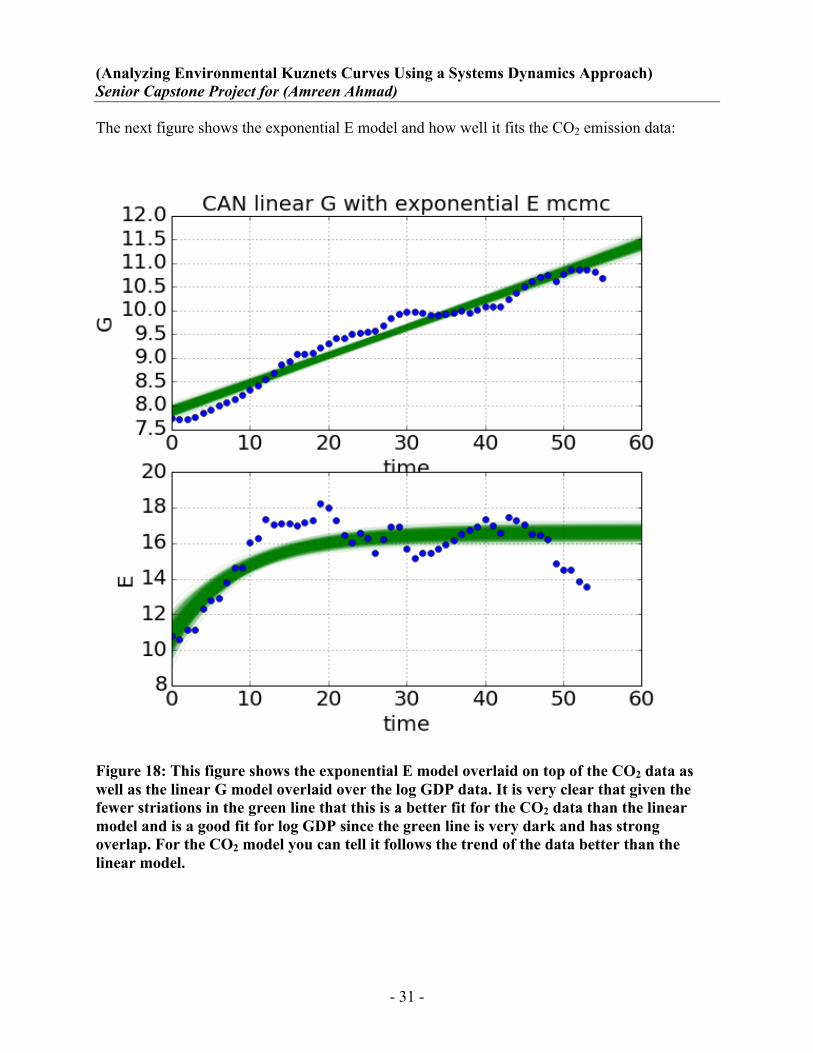
The next figure shows the exponential E model and how well it fits the CO2 emission data:

Figure 18: This figure shows the exponential E model overlaid on top of the CO2 data as well as the linear G model overlaid over the log GDP data. It is very clear that given the fewer striations in the green line that this is a better fit for the CO2 data than the linear model and is a good fit for log GDP since the green line is very dark and has strong overlap. For the CO2 model you can tell it follows the trend of the data better than the linear model.


- 32 -

This last figure shows the fit of the feedback model for E as well as the linear G model:

Figure 19: This figure shows the feedback E model overlaid on top of the CO2 data as well as the linear G model overlaid over the log GDP data. It is very clear that given the fewer striations in the green line that this is a better fit for the CO2 data than the linear model and is a good fit for log GDP since the green line is very dark and has strong overlap. For the CO2 model you can tell it follows the trend of the data better than the linear model, and is better than the exponential model since it follows the


- 33 -

downturn presented in the CO2 data.

Now we will go through the different terms in our equation and determine the parameters/

limits of each as well as whether it is a growth or decay factor. Some of these parameters of

analytical solutions, which are described below.

CO2 Parameters:

B0 =>

E' = b0

E = E0 + b0*t

The b0 term leads to linear growth. It must be a growth factor and must be positive. We refer

to this term henceforth as the linear term in regards to the E term.

B1 =>

E' = b0 + b1*E

E = E0 * eb1*t

This term leads to exponential growth in relation to time therefore it is a growth factor. It

must be negative in order to allow for a downturn that exists in the hypothetical EKC. In

order to have the initial growth we would need a term that is larger than this one that would

eventually be cancelled out through time. This term is referred to henceforth as the

exponential E term.


- 34 -

B4 =>

E' = b0 + b4*E*G

This is one of the most significant parameters we are looking at as it is the feedback term.

This is the term that allows for the downturn in the curve leading to the downward shaped U

curve indicative of an EKC. It must be negative in order for it to lead to the shape we are

looking for. We refer to this parameter as the feedback term throughout the paper. It is

masked at low levels of GDP but then eventually due to the magnitude of the E*G

relationship, it causes the downward turn in the curve.

GDP Parameters:

A0 =>

G' = a0

G’ = G0 + a0*t

This term is related to growth as well and must be positive. This term is referred to henceforth as

the linear G term and it is positive and present in every model as log GDP exhibits linear trends.

This is a growth factor.

A1 =>

G' = a0 + a1*G

This term is the exponential term with respect to GDP. We do not use it often but it is a

parameter we explored initially. This too is a growth factor.

A4 =>


- 35 -

G' = a0+a4*E*G

This term is the feedback term with respect to GDP. It is a decay factor and leads to the

downturn as the E*G value becomes larger.

Bayesian Information Criterion:

Next we will get into the Bayesian Information Criterion (BIC) which is the concept we will be

using to determine the efficacy of our models. The model with the lowest BIC is the one that is

preferred. As you add more parameters, the likelihood of the fit can increase but you are

penalized for adding more parameters. The model with added parameters has to have a better fit

to justify the penalties. In general, the lower the BIC, the better.

The Process in Python:

We used Python notebooks to explore our models. We started with one set of data for the USA

and looked at the GDP vs. CO2 data for that country. We used the equation mentioned in the

methodology section and changed parameter values by hand that would fit the data best. From

there, we used the MCMC method to find the distributions of parameter values that worked well.

We then used those distributions to be able to create an automation notebook from which we

would then run the data of the 200 countries. We used the distributions as values for the different

parameters and then ran the automation that would run the data for all of the different values for

the different models we had created. Each model had a few defined parameters that it would use.

We then collected the results and graphed the BIC’s against one another for different models.


- 36 -

RESULTS AND DISCUSSION

Visualization of Results- BIC Model Comparison:

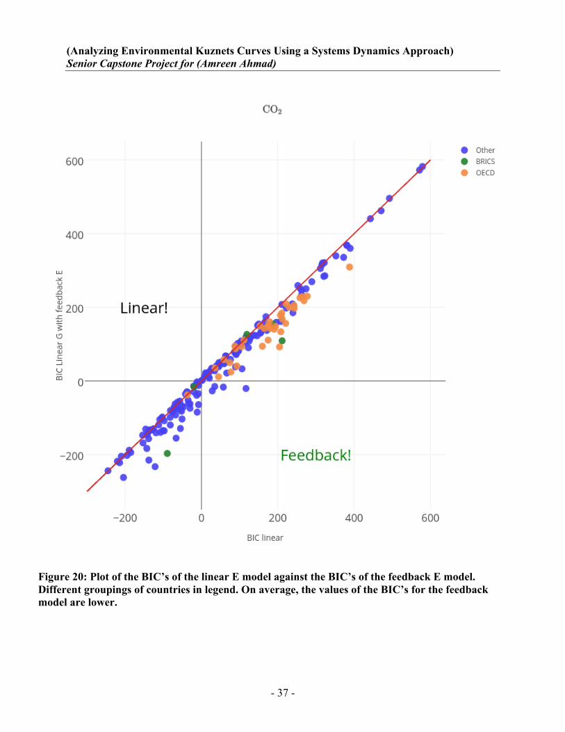
This first graph, Figure 20, plots the BIC’s of the linear model against the BIC’s of the CO2

feedback model. We put a y=x line on the graph to split it in half and visually represent the

differences. Note that points on the line mean that the BIC for the model plotted on the y-axis is

the same as the BIC for the model plotted on the x-axis – they are equivalently good models.

Likewise, points above the line favor the x-axis model and points below the line favor the y-axis

model. As is visible in the graph, the feedback model BIC’s tend to be lower on average than the

linear model BIC’s. This shows that there is some evidence of the Kuznets effect existing. Also,

the majority of the OECD countries are below the y=x line which also shows that there is

evidence of a Kuznets effect existing for those countries data.


- 37 -

Figure 20: Plot of the BIC’s of the linear E model against the BIC’s of the feedback E model. Different groupings of countries in legend. On average, the values of the BIC’s for the feedback model are lower.


- 38 -

The next graph, Figure 21, plots the BIC’s of the exponential model and BIC’s of the feedback

model against each other. On average, the feedback model BIC’s are lower than the exponential

model BIC’s. This graph also shows that there is some evidence of the Kuznets effect existing.


- 39 -

Figure 21: Plot of the values of the BIC of the feedback E model against the values of the BIC of the exponential E model. Different groupings of countries in legend. On average, the feedback model BIC’s are lower.


- 40 -

The next graph, Figure 22, plots the BIC’s of the linear model and BIC’s of the model with

feedback in the G and E terms against each other. On average, the double feedback model BIC’s

are lower than the exponential model BIC’s. This graph also shows that there is some evidence

of the Kuznets effect existing.


- 41 -

Figure 22: Plot of the values of the BIC of the feedback G/E model against the values of the BIC of the feedback E model. Different groupings of countries in legend. On average, the model of feedback G/E has lower BIC’s.


- 42 -

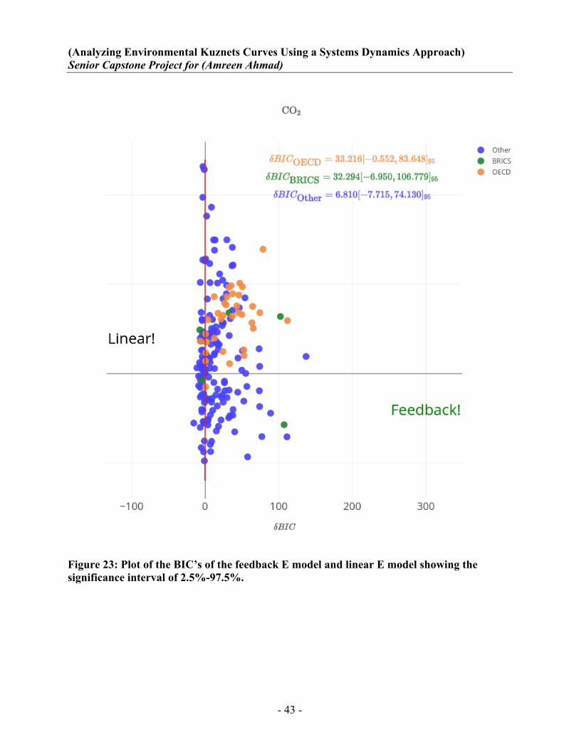
We can also plot the data with the 45 degree line vertically, that would mean a vertical y=x line

in an attempt to more easily visualize the differences between models. The following graphs,

figures 23-25, show the difference in the BIC values on the x-axis for two models with a vertical

y=x line. Deviations from the vertical denote a better fit for one of the models, labeled on the

plot itself. Also shown are the 2.5% and 97.5% interval ranges for these differences to help

determine if these differences are significant. The data is skewed right in favor of the feedback

model showing weak evidence of the Kuznets effect but it is not significant evidence.


- 43 -

Figure 23: Plot of the BIC’s of the feedback E model and linear E model showing the significance interval of 2.5%-97.5%.


- 44 -

Figure 24: Plot of the BIC’s of the feedback E model and exponential E model showing the significance interval of 2.5%-97.5%.


- 45 -

Figure 25: Plot of the BIC’s of the feedback E model and feedback G/E model showing the significance interval of 2.5%-97.5%.


- 46 -

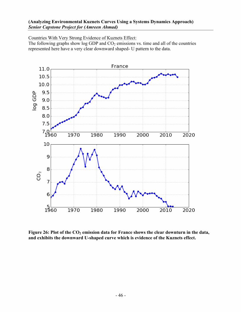
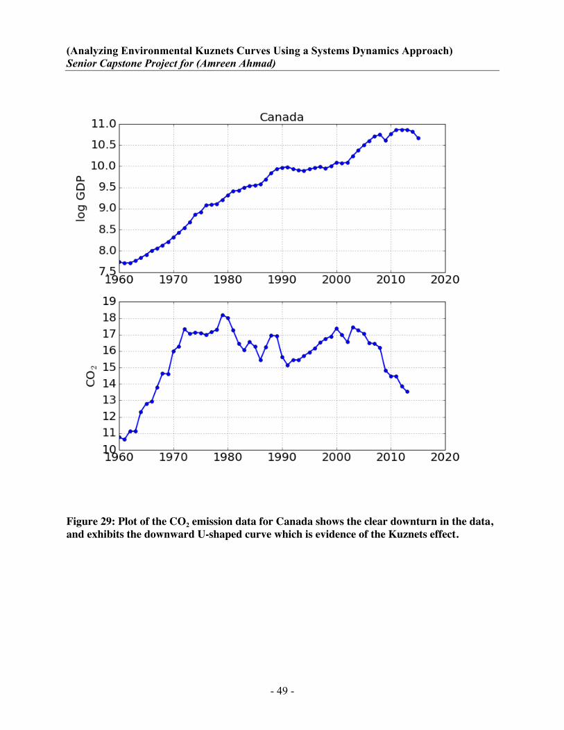
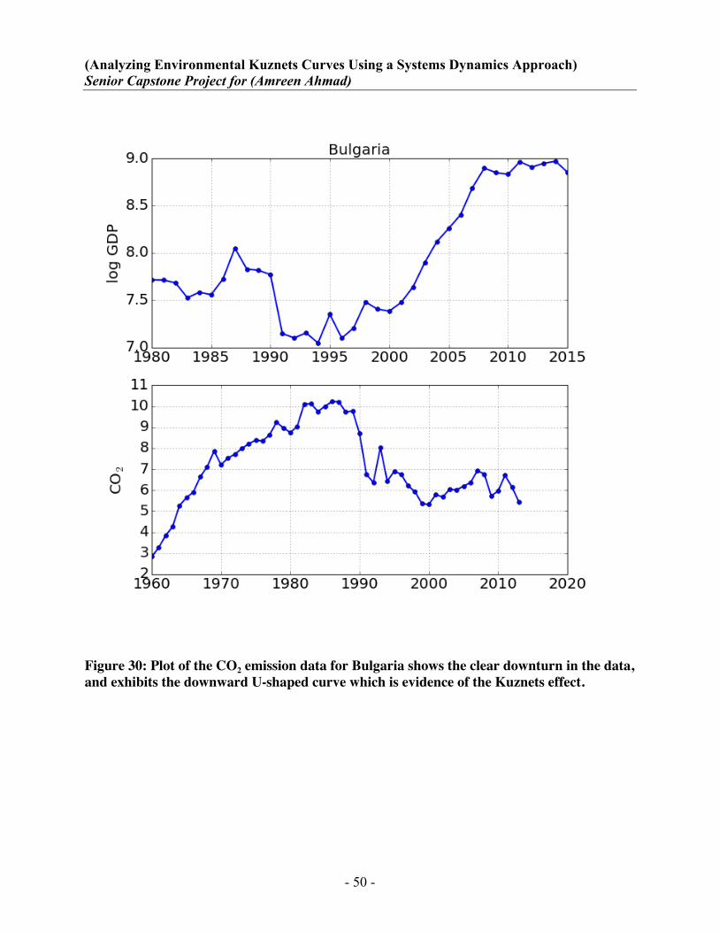
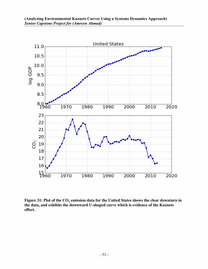
Countries With Very Strong Evidence of Kuznets Effect: The following graphs show log GDP and CO2 emissions vs. time and all of the countries represented here have a very clear downward shaped- U pattern to the data.

Figure 26: Plot of the CO2 emission data for France shows the clear downturn in the data, and exhibits the downward U-shaped curve which is evidence of the Kuznets effect.


- 47 -

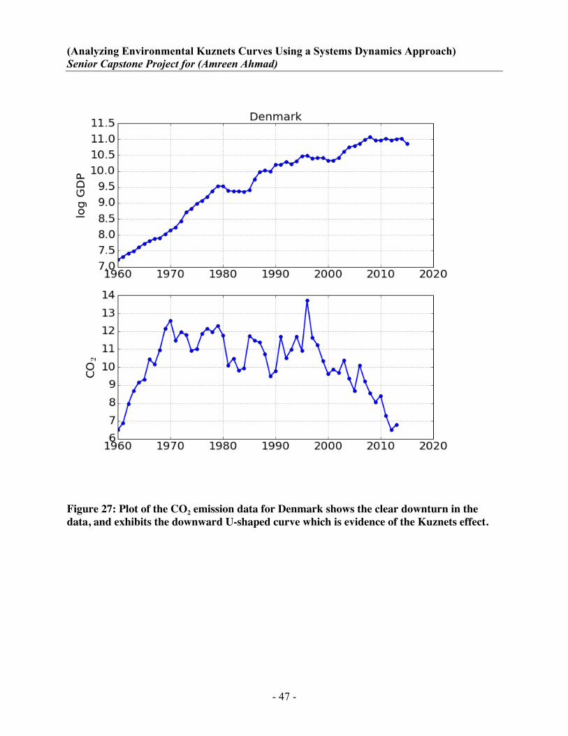
Figure 27: Plot of the CO2 emission data for Denmark shows the clear downturn in the data, and exhibits the downward U-shaped curve which is evidence of the Kuznets effect.


- 48 -

Figure 28: Plot of the CO2 emission data for Switzerland shows the clear downturn in the data, and exhibits the downward U-shaped curve which is evidence of the Kuznets effect.


- 49 -

Figure 29: Plot of the CO2 emission data for Canada shows the clear downturn in the data, and exhibits the downward U-shaped curve which is evidence of the Kuznets effect.


- 50 -

Figure 30: Plot of the CO2 emission data for Bulgaria shows the clear downturn in the data, and exhibits the downward U-shaped curve which is evidence of the Kuznets effect.


- 51 -

Figure 31: Plot of the CO2 emission data for the United States shows the clear downturn in the data, and exhibits the downward U-shaped curve which is evidence of the Kuznets effect.


- 52 -

FINAL CONCLUSION:

There is weak but no significant evidence for the Kuznets effect. This effect is more pronounced

in the OECD and BRICS countries but still not significant. We believe the methodology used

here raises new and unique questions regarding the systems dynamics approach and it’s

application to this problem.


- 53 -

References

1. Yandle B, Vijayaraghavan M, Bhattarai M (2002) The Environmental Kuznets Curve.

Property and Environment Research Center 2(1):1–21.

2. Grossman G, Krueger A (1995) Economic Growth and the Environment. The Quarterly

Journal of Economics:353–376.

3. Ranganathan S, Swain R Analysing Mechanisms for Meeting Global Emissions Target - A

Dynamical Systems Approach.

4. Bernard J-T, Gavin M, Khalaf L, Voia M (2015) Environmental Kuznets Curve: Tipping Points, Uncertainty and Weak Identification. Springer Science and Business Media Dordrecht 60:285–315. 5. Robalino-Lopez A, Garcia-Ramos J-E, Golpe A, Mena-Nieto A (2014) System Dynamics Modelling and the Environmental Kuznets Curve in Ecuador (1980-2025). Elsevier 67:923–931.

6. Coelho F, Codeco C, Gomes M (2011) A Bayesian Framework for Parameter Estimation in Dynamical Models. Plos One 6(5):1–6.

7. Wang S, Fu Y, Zhang Z Population Growth and the Environmental Kuznets Curve. Elsevier 36:146–165.

8. Farhani S, Mrizak S, Chaibi A, Rault C (2014) The Environmental Kuznets Curve and Sustainability: A Panel Data Analysis. Elsevier 71:189–198.

9. Chow G, Li J (2014) Environmental Kuznets Curve: Conclusive Econometric Evidence for CO2. Pacific Economic Review 19(1):1–7.

10. Skaza J, Blais B (2013) The Relationship between Economic Growth and Environmental

Degradation: Exploring Models and Questioning the Existence of an Environmental Kuznets

Curve.


- 54 -

11. Bilgili F, Kocak E, Bulut U (2016) The Dynamic Impact of Renewable Energy Consumption on CO2 Emissions: A Revisited Environmental Kuznets Curve Approach. Elsevier 54:838–845.

12. Akca H, Ozturk I, Karaca C (2012) Economic Development and Environment Pollution in High and Middle Income Countries: A Comparative Analysis of Environmental Kuznets Curve. Actual Problems of Economics 11(137):238–247.

13. Jula D, Dumitrescu C-I, Lie I-R, Dobrescu R-M (2015) Environmental Kuznets curve. Evidence from Romania. Theoretical and Applied Economics 22(602):85–96.

14. Kim KH (2013) Inference of the Environmental Kuznets Curve. Applied Economics Letters 20:119–122.

Analyzing Environmental Kuznets Curves Using a Systems ...

Documents

Transcript of Analyzing Environmental Kuznets Curves Using a Systems ...