Analyzing and modelling exchangerate data using VAR framework

Rokas Serepka

Royal Institute of Technology

A thesis submitted for the degree of

Master in Mathematical Statistics and Financial Mathematics

2012

Acknowledgements

I would like to thank KTH for giving me valuable education in field of financial

mathematics. Especially professor Tobias Rydn for his ideas, guidance and

patience during the time of my theses project.

I also would like to thank my family Lina and Ula for being there for me and

never stopping supporting me.

Abstract

In this report analysis of foreign exchange rates time series are performed. First,

triangular arbitrage is detected and eliminated from data series using linear

algebra tools. Then Vector Autoregressive processes are calibrated and used to

replicate dynamics of exchange rates as well as to forecast time series. Finally,

optimal portfolio of currencies with minimal Expected Shortfall is formed using

one time period ahead forecasts.

Contents

1 Introduction 1

2 Theoretical background 2

2.1 Linear Algebra . . . . . . . . . . . . . . . . . . . . . . . . . . . . . . . . . . 2

2.2 Time series . . . . . . . . . . . . . . . . . . . . . . . . . . . . . . . . . . . . 4

2.3 Portfolio optimization . . . . . . . . . . . . . . . . . . . . . . . . . . . . . . 7

3 Time series under study 10

4 Data projection 12

5 VAR modelling 14

6 Portfolio optimization 16

7 Conclusions 18

Bibliography 19

i

1 Introduction

Foreign exchange market is the largest financial market in the world [5]. With daily turnover

of $4 trillion, which makes it also most liquid one. Market grew by 20% from 2007 to 2010

and 51% since 2004. Spot rate trades increased from $1 trillion to $1.5 trillion from 2007 to

2010 which makes it biggest part of total increase for that period and making it 37.4% of

total turnover [1]. Therefore analysis of spot rates time series, arbitrage opportunities and

portfolio optimization is an interesting and relevant topic. Daily data is easily accessible

from the Internet and analysis can be carried out.

In Chapter 2 theoretical aspects, necessary for this work, are covered. Chapter will start

with linear algebra, which is needed for data preprocessing. Later projection matrices and

pesudoinvers are defined as they are of biggest interest for this work. Triangular arbitrage

will be introduced and linear constraints matrix with respect to arbitrage will be set up.

Vector Autoregressive (VAR) process and toolbox of its estimation, order selection and

stability testing methods will be presented later. Chapter ending with risk measure and

portfolio optimization with these measures.

Chaper 3 and 4 will present data for exchange rates under consideration and its main

qualities (series plots and correlation heat map). Then arbitrage elimination using linear

constraints matrix and linear projection will be done and results will be compared with data

before projection. In addition variances of original and projected data will be compared.

Chapter 5 covers VAR analysis, estimation and forecasting. From this part, just USD

exchange rates will be used. This will be done to have a reference currency and measure

portfolio value in next chapter. The USD is chosen as reference currency as it accounts

for as much as 84.9% (out of 200%) of daily trading turnover and can be still seen as the

biggest currency in the world. Thus in Chapter 6 forecasts from Chapter 5 are used for

portfolio optimization and trading simulations for currency portfolios.

1

2 Theoretical background

2.1 Linear Algebra

First, I will present some basic results from linear algebra. Most of them can be found, in

more details and examples, in the book by Axler (1997 [8]). These results will be used to

eliminate triangular arbitrage opportunities in downloaded data.

Definition 2.1 A vector space is a set V along with an addition on V and a scalar

multiplication on V such that the following properties hold:

commutativity u+ v = v + u, for all u, v ∈ V ,

associativity (u + v) + w = u + (v + w) and (ab)v = a(bv) for all u, v, w ∈ V and all

a, b ∈ R,

additive identity there exists an element 0 ∈ V such that v + 0 = v for all v ∈ V ,

additive inverse for every v ∈ V , there exists w ∈ V such that v + w = 0,

multiplicative identity 1v = v for all v ∈ V ,

distributive properties a(u + v) = au + av and (a + b)u = au + bu for all a, b ∈ Rand all u, v ∈ V .

Definition 2.2 A nonempty subset U of a vector space V is a subspace of V if

• x, y ∈ U ⇒ x+ y ∈ U ,

• x ∈ U ⇒ αx ∈ U,∀α ∈ R.

Data for daily exchange rates can be seen as vectors and all these vectors form a vector

space. Assume there are n currencies and let us denote them as ai, i = 1 . . . n. Then there

will be

(n

2

)= n(n− 1)/2 exchange rates

aiaj

, i, j = 1 . . . n stored in vectors

x =

(a1a2,a1a3,a1a4, . . . ,

a1an,a2a3,a2a4, . . . ,

an−1an

)T. (2.1)

Definition 2.3 A list (v1, . . . , vm) of vectors in V is called linearly independent if the only

choice of a1, . . . , am ∈ R that satisfies a1v1 + · · ·+ amvm = 0 is a1 = · · · = am = 0.

Definition 2.4 A basis of V is a list of vectors in V that is linearly independent and spans

V .

2

Definition 2.5 An inner product on V is a function that takes each ordered pair (u, v)

of elements of V to a number 〈u, v〉 ∈ R and has the following properties:

positivity 〈v, v〉 ≥ 0 for all v ∈ V ,

definiteness 〈v, v〉 = 0 if and only if v = 0,

additivity in first slot 〈u+ v, w〉 = 〈u,w〉+ 〈v, w〉 for all u, v, w ∈ V ,

homogeneity in first slot 〈av, w〉 = a〈v, w〉 for all a ∈ R and all v, w ∈ V ,

symmetry 〈v, w〉 = 〈w, v〉 or all v, w ∈ V .

Definition 2.6 For v ∈ V the norm of v, denoted ‖v‖ , by

‖v‖ =√〈v, v〉.

Definition 2.7 Two vectors u, v ∈ V are said to be orthogonal if 〈u, v〉 = 0.

Definition 2.8 A list of vectors is called orthonormal if the vectors in it are pairwise

orthogonal and each vector has norm 1. In other words, a list (e1, . . . , em) of vectors in V

is orthonormal if 〈ej , ek〉 equals 0 when j 6= k and equals 1 when j = k (for j, k = 1, . . . ,m).

Definition 2.9 An orthonormal basis of V is an orthonormal list of vectors in V that

is also a basis of V .

Now let’s go back to exchange rates. Exchange rates can be expressed in terms of each

other

(aiaj

)=

(aiak

)·(akaj

). If one of these relationships does not hold, there will be

triangular arbitrage opportunity. Which basically means, that with taking no risk, money

can be made, by buying and instantly selling currencies [2]. In practice, such opportunities

exist, even though they can be neglected due to transactions costs. Nevertheless, it would

be nice to take them away form data before modelling. Here is where linear algebra steps

in. Relationships

(aiaj

)=

(aiak

)·(akaj

)can be transformed to log-scale to make them

linear ln

(aiaj

)= ln

(aiak

)+ ln

(akaj

). Linear relationships can be rewritten in matrix form

AxT = 0 (2.2)

where

A =

−1{1,2} 1{1,3} 0 0 · · · −1{2,3} 0 · · · · · · 0

−1{1,2} 0 1{1,4} 0 · · · 0 −1{2,4} 0 · · · 0...

......

......

......

......

...0 −1{i,k} · · · 0 1{i,j} 0 · · · −1{k,j} 0 · · ·...

......

......

......

......

...

(2.3)

and x is defined as in (2.1). After having constructed matrix A it is possible to project data

onto the subspace where the linear constraints do hold.

3

Definition 2.10 Let A be an m× n matrix. The null and range space of A are the set of

vectorsN(A) :=

{x ∈ Rn|AxT = 0

}R(A) :=

{AxT ∈ Rm|x ∈ Rn

}Next definition is taken from [3].

Definition 2.11 For v ∈ V , let v = m+ n, where m ∈ U and n ∈ U⊥.

• m is called the orthogonal projection of v onto U .

• The projector PU onto U along U⊥ is called the orthogonal projector onto U .

• PU is the unique linear operator such that PU = m

Theorem 2.1 Let A be and m × n matrix. The pseudo inverse A+ is an n × m matrix

satisfying:

i. A+A = P is the orthogonal projector P : Rn → N(A)⊥ and AA+ = P is the orthogonal

projector P : Rm → R(A).

ii. The following formulas hold:

(a) A+A = (A+A)T

(b) AA+ = (AA+)T

(c) AA+A = A

(d) A+AA+ = A+

Proof of Theorem 2.1 can be found in [9]. For my purposes I will need the orthonormal

basis of matrix A and its pseudo-inverse.

2.2 Time series

Modelling the big amount of related time series individually is not an easy task if possible

at all. Using multivariate models makes it much easier. It also takes into account the

correlation between variables, which is very important with any amount of time series

under analysis. I will consider Vector Autoregressive (VAR) models for my data. Most

of the multivariate time series theory is taken from Lutkepohl (2005 [4]).

A VAR model of order p (VAR(p)) can be written as

yt = ν +A1yt−1 + · · ·+Apyt−p + ut, t = 0, 1, . . . (2.4)

where yt = (y1t, . . . , yKt)′ is a random vector, K is the process dimension, the Ai are

coefficient matrices, ν = (ν1, . . . , νK)′ is fixed vector of terms allowing for the possibility of

nonzero mean and ut = (u1t, . . . , uKt)′ is white noise with covariance matrix Σu.

First thing to do, when analysing the process itself, is to check its stability. If the

process is not stable it can explode or produce irrelevant results. The process in (2.4) is

stable, if its reverse characteristic polynomial has no roots in and on the complex unit circle

det(IK −A1z − · · · −Apzp) 6= 0 for |z| ≤ 1. (2.5)

4

For computational purposes I have used another (equivalent) definition of stability from

Tsay (2002 [10]). The VAR(p) can be written down as a VAR(1)

Yt = ν + AYt−1 + Ut (2.6)

where

Yt =

ytyt−1

...yt−p+1

, ν =

ν0...0

,

A =

A1 A2 . . . Ap−1 ApIK 0 . . . 0 00 IK . . . 0...

. . ....

...0 0 . . . IK 0

, Ut =

ut0...0

..

The process (2.6) will be stable when all eigenvalues of A are less than 1 in the modulus.

Let’s assume that time series y1, . . . , yT of currency rates are available and are generated

by a stable VAR(p) process as in (2.4), but now coefficients ν,Ai, and Σu are unknown.

By following [4], estimates can be achieved using multivariate least squares (LS) and

maximum likelihood (ML) methods. There will be p presample vectors y−p+1, . . . , y0 of

data needed and we define

µ =1

T

T∑t=1

yt

Y := (y1, . . . , yT ) (K × T ),B := (ν,A1, . . . , Ap) (K × (Kp+ 1)),

Zt :=

1yt...

yt−p+1

((Kp+ 1)× 1),

U := (Z0, . . . , ZT1) (K × T ),A := (A1, . . . , Ap) (K ×Kp),Y 0 := (y1, . . . , yT − µ) (K × T )

Y 0t :=

yt − µ...

yt−p+1 − µ

(Kp+ 1),

X := (Y 00 , . . . , Y

0T−1)

(2.7)

Using this notation (2.6) can be rewritten as

5

Y = BZ + U.

LS and ML estimates of B and Σu can be written down in a simple and nice matrix way

B = Y ZT (ZZT )−1

Σu =1

T(Y − BZ)(Y − BZ)T .

(2.8)

The log-likelihood function can be written as

Σu = −KT2

ln2π − T

2ln|Σu| −

1

2tr[(Y 0 −AX)′Σ−1u (Y 0 −AX)] (2.9)

where tr is matrix trace. Maximization of the log-likelihood function gives ML estimates.

It is shown in [4], that these estimates are asymptotically equivalent to the least squares

estimates. For my estimates I will use (2.8) for B and (2.9) for Σu.

In the discussion up until now, it was assumed that the VAR order p is known. In

practice, however, it is almost always unknown. I will consider a few methods for order

indication and selection. The principle behind all of them is: choose an upper limit of VAR

order, fit model to the data and compare fitted models.

The likelihood ratio test compares the maxima of the log-likelihood function over

the unrestricted and restricted parameter space. Test statistics have asymptotic χ2(K2)

distribution. In VAR case, given upper order bound M the sequence of null and alternative

hypotheses are tested:

H i0 : AM−i+1 = 0 versus H i

1 : AM−i+1 6= 0 |AM = · · · = AM−i+2 = 0, for i = 1 : M

The sequence is terminated when H i0 is rejected and order p = M − i + 1 is chosen. The

test statistic for the i’th null hypothesis is

λLR(i) = T [ln|Σu(M − i)| − ln|Σu(M − i+ 1)|]

For prediction purposes one would like to choose such an order that prediction error is

minimized. As one step ahead prediction error is determined by the covariance matrix of

residuals Σu (see [4]) quite a few criteria have been developed based on it. The Akaikes

Information Criterion (AIC), final prediction error (FPE), Hanna-Quinn criterion

(HQ) and Schwarz criterion (SC) are few of the most popular ones in practice.

AIC(m) = ln|Σu(m)|+ 2mK2

T,

FPE(m) =

[T +Km+ 1

T −Km− 1

]K|Σu(m)|,

HQ(m) = ln|Σu(m)|+ 2lnlnT

TmK2,

SC(m) = ln|Σu(m)|+ lnT

TmK2.

AIC and FPE tend to overestimate the process order with positive probability while

HQ and SC seem to be consistent. Nevertheless it does not necessarily mean that AIC and

FPE are worst. On the contrary, let’s say, for predicting purposes they suit better.

6

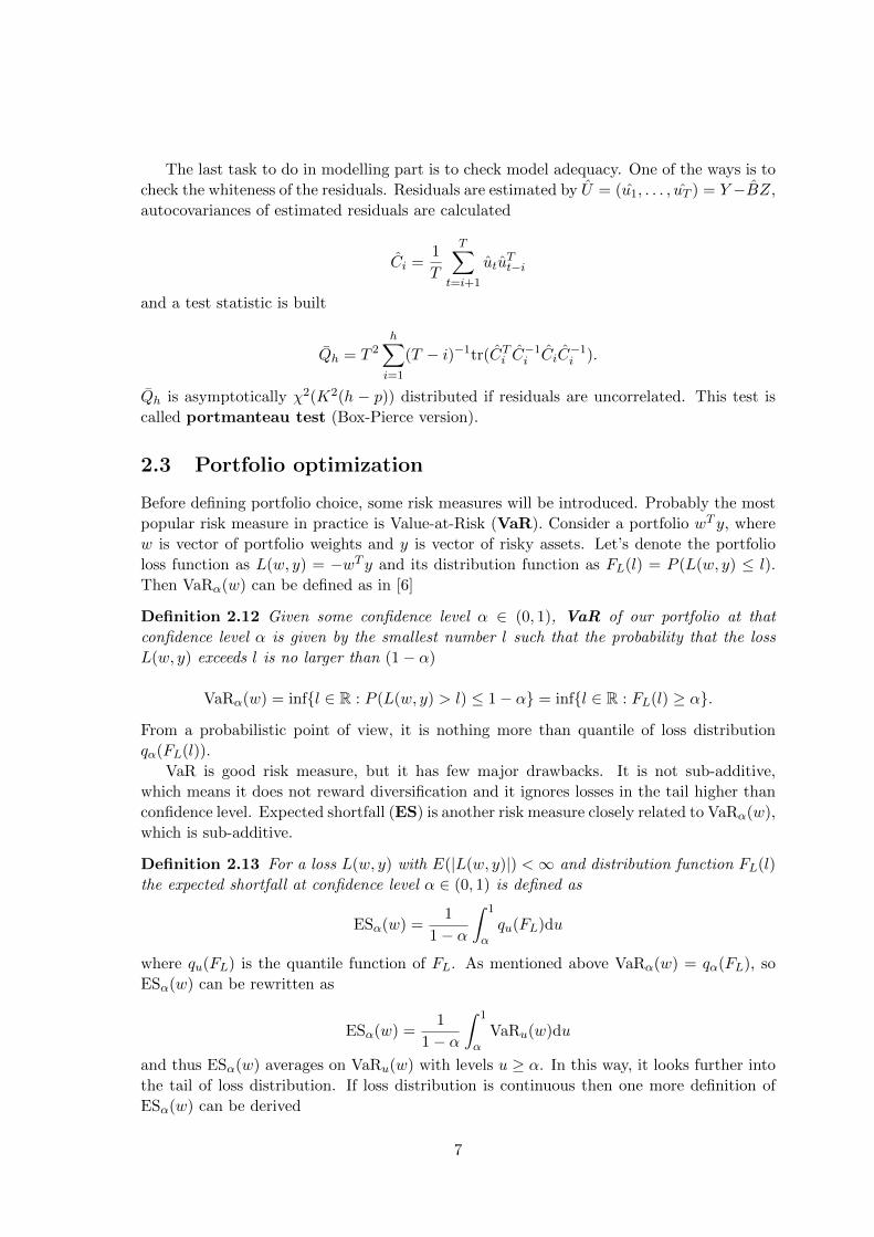
The last task to do in modelling part is to check model adequacy. One of the ways is to

check the whiteness of the residuals. Residuals are estimated by U = (u1, . . . , uT ) = Y −BZ,

autocovariances of estimated residuals are calculated

Ci =1

T

T∑t=i+1

utuTt−i

and a test statistic is built

Qh = T 2h∑i=1

(T − i)−1tr(CTi C−1i CiC−1i ).

Qh is asymptotically χ2(K2(h − p)) distributed if residuals are uncorrelated. This test is

called portmanteau test (Box-Pierce version).

2.3 Portfolio optimization

Before defining portfolio choice, some risk measures will be introduced. Probably the most

popular risk measure in practice is Value-at-Risk (VaR). Consider a portfolio wT y, where

w is vector of portfolio weights and y is vector of risky assets. Let’s denote the portfolio

loss function as L(w, y) = −wT y and its distribution function as FL(l) = P (L(w, y) ≤ l).

Then VaRα(w) can be defined as in [6]

Definition 2.12 Given some confidence level α ∈ (0, 1), VaR of our portfolio at that

confidence level α is given by the smallest number l such that the probability that the loss

L(w, y) exceeds l is no larger than (1− α)

VaRα(w) = inf{l ∈ R : P (L(w, y) > l) ≤ 1− α} = inf{l ∈ R : FL(l) ≥ α}.

From a probabilistic point of view, it is nothing more than quantile of loss distribution

qα(FL(l)).

VaR is good risk measure, but it has few major drawbacks. It is not sub-additive,

which means it does not reward diversification and it ignores losses in the tail higher than

confidence level. Expected shortfall (ES) is another risk measure closely related to VaRα(w),

which is sub-additive.

Definition 2.13 For a loss L(w, y) with E(|L(w, y)|) <∞ and distribution function FL(l)

the expected shortfall at confidence level α ∈ (0, 1) is defined as

ESα(w) =1

1− α

∫ 1

αqu(FL)du

where qu(FL) is the quantile function of FL. As mentioned above VaRα(w) = qα(FL), so

ESα(w) can be rewritten as

ESα(w) =1

1− α

∫ 1

αVaRu(w)du

and thus ESα(w) averages on VaRu(w) with levels u ≥ α. In this way, it looks further into

the tail of loss distribution. If loss distribution is continuous then one more definition of

ESα(w) can be derived

7

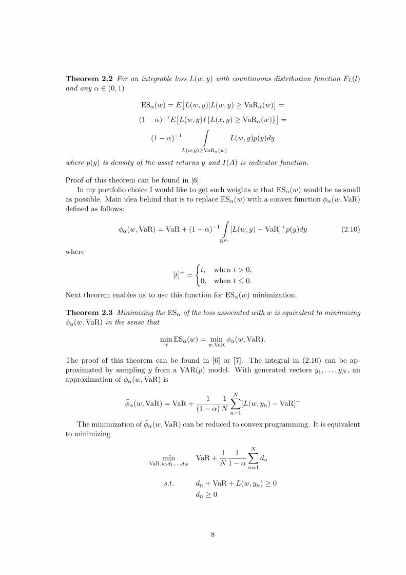
Theorem 2.2 For an integrable loss L(w, y) with countinuous distribution function FL(l)

and any α ∈ (0, 1)

ESα(w) = E[L(w, y)|L(w, y) ≥ VaRα(w)

]=

(1− α)−1E[L(w, y)I{L(x, y) ≥ VaRα(w)}

]=

(1− α)−1∫

L(w,y)≥VaRα(w)

L(w, y)p(y)dy

where p(y) is density of the asset returns y and I(A) is indicator function.

Proof of this theorem can be found in [6].

In my portfolio choice I would like to get such weights w that ESα(w) would be as small

as possible. Main idea behind that is to replace ESα(w) with a convex function φα(w,VaR)

defined as follows:

φα(w,VaR) = VaR + (1− α)−1∫Rm

[L(w, y)−VaR]+p(y)dy (2.10)

where

[t]+ =

{t, when t > 0,

0, when t ≤ 0.

Next theorem enables us to use this function for ESα(w) minimization.

Theorem 2.3 Minimizing the ESα of the loss associated with w is equivalent to minimizing

φα(w,VaR) in the sense that

minw

ESα(w) = minw,VaR

φα(w,VaR).

The proof of this theorem can be found in [6] or [7]. The integral in (2.10) can be ap-

proximated by sampling y from a VAR(p) model. With generated vectors y1, . . . , yN , an

approximation of φα(w,VaR) is

φα(w,VaR) = VaR +1

(1− α)

1

N

N∑n=1

[L(w, yn)−VaR]+

The minimization of φα(w,VaR) can be reduced to convex programming. It is equivalent

to minimizing

minVaR,w,d1,...,dN

VaR +1

N

1

1− α

N∑n=1

dn

s.t. dn + VaR + L(w, yn) ≥ 0

dn ≥ 0

8

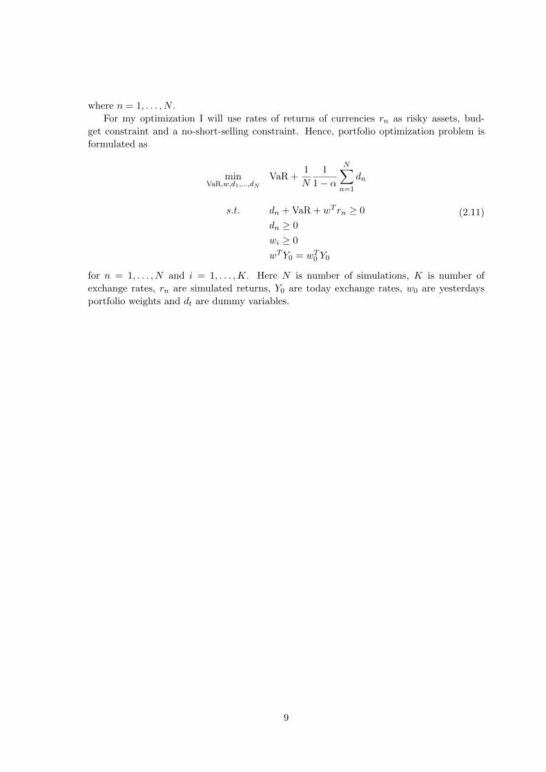
where n = 1, . . . , N .

For my optimization I will use rates of returns of currencies rn as risky assets, bud-

get constraint and a no-short-selling constraint. Hence, portfolio optimization problem is

formulated as

minVaR,w,d1,...,dN

VaR +1

N

1

1− α

N∑n=1

dn

s.t. dn + VaR + wT rn ≥ 0

dn ≥ 0

wi ≥ 0

wTY0 = wT0 Y0

(2.11)

for n = 1, . . . , N and i = 1, . . . ,K. Here N is number of simulations, K is number of

exchange rates, rn are simulated returns, Y0 are today exchange rates, w0 are yesterdays

portfolio weights and dt are dummy variables.

9

3 Time series under study

For modelling purposes multivariate data of exchange rates will be needed. 20 currencies

have been chosen and daily data of their exchange rates have been downloaded.

USD US Dollar INR Indian RupeeCAD Canadaian Dollar IDR Indonesian RupeeEUR European Euro KRW South Korean WonGBP Great Britain Pound MXN Mexican PesoJPY Japanese Yen NOK Norwegian KroneARS Argentine Peso RUB Russia RubleAUD Australian Dollar ZAR South Africa RandBRL Brazilian Real SEK Swedish KronaCNY Chinese Yuan CHF Swiss FrankHKD Hong Kong Dollar TRY Turkish Lira

Table 3.1: Currencies

Data is organised in the following manner to match the vector in (2.1)(USD

CAD,

USD

EUR,

USD

GBP, . . . ,

USD

TRY,CAD

EUR,CAD

GBP, . . . ,

CHF

TRY

)T.

(a) All rates (b) USD rates

Figure 3.1: Correlation between exchange rates. White arearepresents uncorrelated parts, while black area representsstrong (both positively and negatively) correlation.

This vector includes 190 exchange rates. Time period for data is between 2007-10-16 and

2011-10-16, which is 1004 consecutive trading days. Thus a 190-by-1004 matrix of data

10

is formed. After projection (next chapter) data will be divided into two samples: one for

model estimation, and another for forecasting and portfolio performance comparison. Data

will be also scaled to weekly (every 5’th trading day) and bi-weekly (every 10’th trading

day) samples, to see how exchange rate dynamics change for longer time periods. Some

examples of time series from the data set are plotted in Figure 3.2. The correlation matrix

of all 190 exchange rates and of the 19 first ones(USDCAD , . . . ,

USDTRY ,

)are plotted in Figure 3.1.

It can be seen that data is strongly correlated, which supports the choice of multivariate

modelling.

Figure 3.2: Daily data of exchange rates: USDCAD ,

USDEUR ,

USDGBP

(a) Weekly data (b) Bi-weekly

Figure 3.3: Weekly and bi-weekly data of exchange rates: : USDCAD ,

USDEUR ,

USDGBP

11

4 Data projection

As it was indicated before, a linear projection will be used to eliminate triangular arbitrage

opportunities. In Chapter 2 the matrix A of linear constraints (2.3) was constructed. In

our case (with 190 exchange rates) A ∈ R1140×190. We would like to project data to the

space where the linear constraints hold, hence the null space of A. One way of achieving it

is to find orthonormal basis (N) for the null space of A and its pseudo inverse N+. Now

matrix N is in R190×19, N+ ∈ R19×190 and projection PN(A) = NN+ ∈ R190×190.

Before applying the projection, our data matrix is log-scaled D = log(Data) and pre-

multiplied with matrix A to see, if there exists any arbitrage at all. Biggest arbitrage is

1.0532 × 10−4 which probably can be neglected due to transaction costs, but still exists.

Average arbitrage would be 1.3072× 10−5.

After projection is applied (PN(A)D), the resulting matrix is premultiplied with A. The

biggest arbitrage now is 4.3521× 10−14 and average would be 5.7346× 10−15. Such a small

number is approximately equal to zero in both economical and mathematical sense and is

due to rounding errors.

As P is an orthogonal projection and by using Definition 2.11 the following is true

||v||2 = ||Pv + n||2 = ||Pv||2 + 〈Pv, n〉+ 〈n, Pv〉+ ||n||2

= ||Pv||2 + ||n||2 ≥ ||Pv||2 ⇒ ||Pv||2 ≤ ||v||2 ⇒ 〈Pv, Pv〉 ≤ 〈v, v〉.

If we define 〈X,Y 〉 = E[XY ] and v = X − µ we get

E[(P (X − µ))2] ≤ E[(X − µ)2]⇒PE[(X − µ)2] ≤ E[(X − µ)2]⇒PV ar(X) ≤ V ar(X).

12

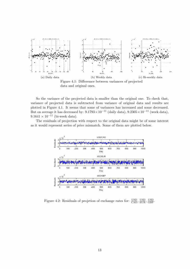
(a) Daily data (b) Weekly data (c) Bi-weekly data

Figure 4.1: Differemce between variances of projecteddata and original ones.

So the variance of the projected data is smaller than the original one. To check that,

variance of projected data is subtracted from variance of original data and results are

plotted in Figure 4.1. It seems that some of variances has increased and some decreased.

But on average it has decreased by: 9.1793×10−11 (daily data), 9.2305×10−11 (week data),

9.1641× 10−11 (bi-week data).

The residuals of projection with respect to the original data might be of some interest

as it would represent series of price mismatch. Some of them are plotted below.

Figure 4.2: Residuals of projetion of exchange rates for: USDCAD ,

USDEUR ,

USDGBP .

13

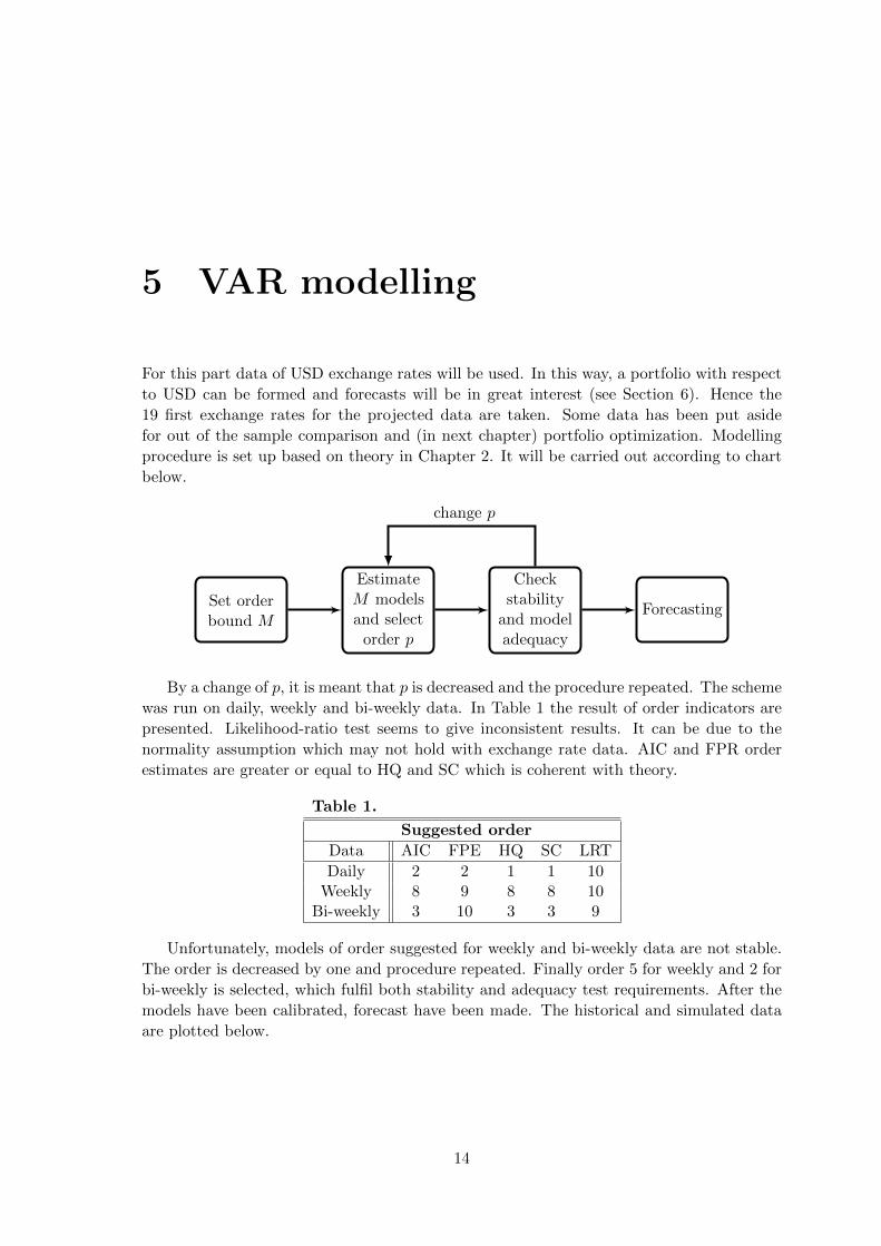
5 VAR modelling

For this part data of USD exchange rates will be used. In this way, a portfolio with respect

to USD can be formed and forecasts will be in great interest (see Section 6). Hence the

19 first exchange rates for the projected data are taken. Some data has been put aside

for out of the sample comparison and (in next chapter) portfolio optimization. Modelling

procedure is set up based on theory in Chapter 2. It will be carried out according to chart

below.

Set orderbound M

EstimateM modelsand select

order p

Checkstability

and modeladequacy

Forecasting

change p

By a change of p, it is meant that p is decreased and the procedure repeated. The scheme

was run on daily, weekly and bi-weekly data. In Table 1 the result of order indicators are

presented. Likelihood-ratio test seems to give inconsistent results. It can be due to the

normality assumption which may not hold with exchange rate data. AIC and FPR order

estimates are greater or equal to HQ and SC which is coherent with theory.

Table 1.

Suggested order

Data AIC FPE HQ SC LRT

Daily 2 2 1 1 10Weekly 8 9 8 8 10

Bi-weekly 3 10 3 3 9

Unfortunately, models of order suggested for weekly and bi-weekly data are not stable.

The order is decreased by one and procedure repeated. Finally order 5 for weekly and 2 for

bi-weekly is selected, which fulfil both stability and adequacy test requirements. After the

models have been calibrated, forecast have been made. The historical and simulated data

are plotted below.

14

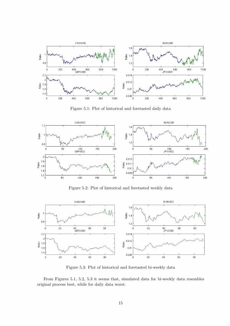
Figure 5.1: Plot of historical and foretasted daily data

Figure 5.2: Plot of historical and foretasted weekly data

Figure 5.3: Plot of historical and foretasted bi-weekly data

From Figures 5.1, 5.2, 5.3 it seems that, simulated data for bi-weekly data resembles

original process best, while for daily data worst.

15

6 Portfolio optimization

A portfolio of foreign currencies with respect to USD is formed. Scenarios one day ahead

are simulated from the VAR(p) model as in Chapter 5. Then optimal portfolio of min-ES as

in (2.11) are obtained. For the first optimization we set wT0 Y0 = 100 which means, that the

initial budget is 100$. Then data used for VAR model simulations is updated with historical

data (adding one day to existing data). Simulations one day ahead are made again and

optimization is repeated. For second and further optimizations the budget is what is left

form yesterday’s investment wT0 Y0.

Same framework is repeated for weekly data (every 5’th trading day) and bi-weekly data

(every 10’th trading day) and plots of portfolio value changes can be seen in Figure 6.1 and

Figure 6.2.

Figure 6.1: Portfolio value change (daily trading)

All portfolios perform similarly start quite well, but end up with a drop. It is due to

bigger negative move in a all 19 USD exchange rates. The average changes of all 19 assets

in last 50 trading days is −5.97%. Naturally the portfolio value will fall as all the assets

fall. In this case, the purpose of a portfolio with minimized risk is to make this fall as small

as possible. From the figures it can be seen, that the portfolio of weekly reallocations has

done best and bi-weekly worst.

16

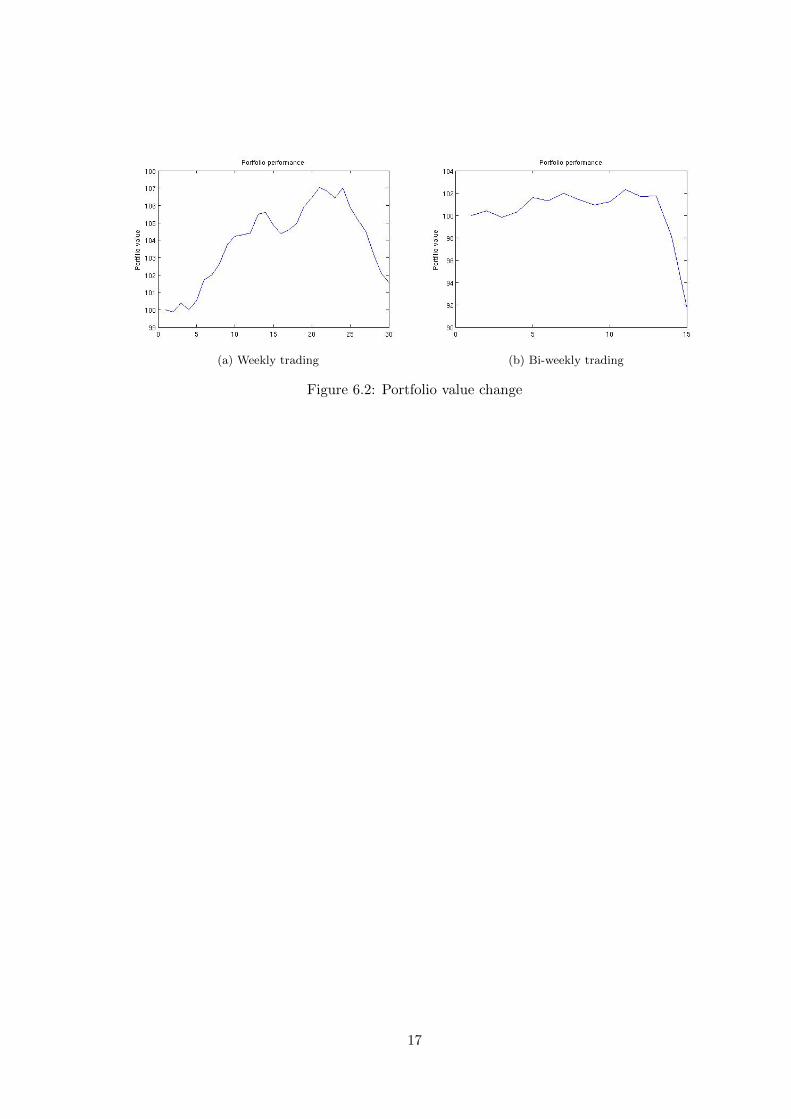
(a) Weekly trading (b) Bi-weekly trading

Figure 6.2: Portfolio value change

17

7 Conclusions

Modelling multivariate date, especially when the dimension is as high as 19, is a quite

complicated task. Main purpose of this report was to implement methods from different

mathematical fields to analyse and model currency data. After doing that some conclusions

on methods performance can be drawn.

First, and probably the most interesting part, is the elimination of triangular arbitrage

from data using linear projection. The matrix representation of linear constraints can be

used not only to transform the data to arbitrage free space, but also to identify arbitrage

opportunities and their values. The arbitrages discovered in this work seem to be too small

to make use of, due to transaction costs. However, currency trading is open 24 hours for

five days a week and is continuous in time. It can be suggested to look into higher frequency

data and apply the same methods. Arbitrages there could be big enough to make profit of.

It might be aslo interesting to analyse residuals of projection.

Biggest difference between modelling univariate and multivariate time series is that in

the univariate case one looks at partial autocorrelation or autocorrelation function for order

indication and in multivariate case it is not possible. Order selection relies on tests and

these differ in purposes and consistency. And even after deciding on which one to use, the

estimated coefficients can produce an unstable model. In the end two out of three model

order have been chosen just by reducing order from indicated one, until a stable process

is obtained. Nevertheless, the estimated models seemed to replicate dynamics of time

series quite well, especially for data with longer time steps. More complicated models like

VARMA, multivariate ARCH or GARCH could potentially improve replication of currency

rates dynamics and should be considered for future studies.

Finally, portfolio of min-ES was estimated using one time step forecasts. All three

portfolios performed quite similarly. The fall in its value is due to general fall in USD

value in world market. Portfolio of weekly reallocations has done best, as it made this fall

smoother, while bi-weekly has done worst. This type of portfolio optimization can searve as

suggestion for trader. Other types of portfolio choices could be considered, combined with

other models for scenarios generation.

18

Bibliography

[1] 2010 Triennial Central Bank Survey. Bank for International Settlements, 2010.

[2] Y. Aiba, N. Hatano, H. Takayasu, K. Marumo, and T. Shimizu. Triangular arbitrage

as an interaction among foreign exchange rates. Physica A, 310:467–479, 2002.

[3] G.H. Golub and C.F. van Loan. Matrix computations (3rd ed.). JHU, 1996.

[4] Luetkepohl H. New Introduction to Multiple Time Series Analysis. Springer, 2005.

[5] M.R. King and D. Rime. The $4 trillion question: what explains FX growth since the

2007 survey? Bank for International Settlements, 2010.

[6] Alexander J. McNeil, Rdiger Frey, and Paul Embrechts. Quantitative Risk Manage-

ment: Concepts, Techniques, and Tools. Princeton Series in Finance, 2005.

[7] R.T. Rockafellar and S. Uryasev. Conditional value-at-risk for general loss distributions.

Journal of Banking & Finance, 26:1443–1471, 2002.

[8] Axler S. Linear Algebra Done Right (2nd ed.). Springer, 1997.

[9] Bulirsch R. Stoer J. Introduction to Numerical Analysis. Springer, 2002.

[10] Ruey S. Tsay. Analysis of Financial Time Series. A Wiley-Interscience publication,

2002.

19