AnalyticalandComputationalStudiesofCorrelations of ... ·...

Commun. Comput. Phys.doi: 10.4208/cicp.OA-2017-0051

Vol. 23, No. 1, pp. 93-117January 2018

Analytical and Computational Studies of Correlations

of Hydrodynamic Fluctuations in Shear Flow

Xin Bian∗,†, Mingge Deng and George Em Karniadakis

Division of Applied Mathematics, Brown University, Providence, Rhode Island 02912,USA.

Received 11 March 2017; Accepted (in revised version) 28 April 2017

Abstract. We study correlations of hydrodynamic fluctuations in shear flow analyt-ically and also by dissipative particle dynamics (DPD) simulations. The hydrody-namic equations are linearized around the macroscopic velocity field and then solvedby a perturbation method in Fourier-transformed space. The autocorrelation func-tions (ACFs) from the analytical method are compared with results obtained from DPDsimulations under the same shear-flow conditions. Up to a moderate shear rate, var-ious ACFs from the two approaches agree with each other well. At large shear rates,discrepancies between the two methods are observed, hence revealing strong addi-tional coupling between different fluctuating variables, which is not considered in theanalytical approach. In addition, the results at low and moderate shear rates can serveas benchmarks for developing multiscale algorithms for coupling of heterogeneoussolvers, such as a hybrid simulation of molecular dynamics and fluctuating hydrody-namics solver, where thermal fluctuations are indispensable.

AMS subject classifications: 76M28, 82C22, 34F05

Key words: Hydrodynamic fluctuations, correlation functions, dissipative particle dynamics,shear flow.

1 Introduction

The complex behavior of many particles plays a significant role in atomic fluids [1, 2],chemical and biological processes [3, 4], granular materials [5], and astrophysics [6]. Onthe one hand, given interparticle potentials, a kinetic-theory type of description from first

∗Corresponding author. Email addresses: [email protected] (X. Bian), mingge [email protected] (M. Deng),george [email protected] (G. E. Karniadakis)†Present address: Lehrstuhl fur Aerodynamik und Stromungsmechanik, Technische Universitat Munchen,85748 Garching, Germany.

http://www.global-sci.com/ 93 c©2018 Global-Science Press

94 X. Bian, M. Deng and G. E. Karniadakis / Commun. Comput. Phys., 23 (2018), pp. 93-117

principles can be formulated, which, however, may be too complex to apply. On the otherhand, if physical quantities vary rather slowly in space and time, a local thermodynamicequilibrium may be valid. Therefore, the system can be represented by continuous hy-drodynamic fields described by the Navier-Stokes-Fourier (NSF) equations, which takeinto account the conservation of mass, momentum and energy. Although such partialdifferential equations (PDEs) are concise and practically powerful, the thermodynamicderivatives and transport coefficients must be obtained from a more fundamental theoryto complete the phenomenological description. Through the seminal efforts of Einstein,Onsager, Callen, Welton, Green, Kubo and many others [1, 7], a general linear responsetheory has been established. Furthermore, the transport coefficients are connected tothe corresponding correlation functions (CFs) of the microscopic fluctuating variables.These connections are all embraced in the fundamental Green-Kubo relations. At equi-librium or small deviations from equilibrium, a systematic connection between the CFsand the hydrodynamics equations has been established for the long wave-length andsmall-frequency hydrodynamic limit [1, 8, 9]. In this hydrodynamic limit, the effects ofthe solvent fluctuations on suspended Brownian particles have also been studied exten-sively [10]. A further extension for small wave-length of the fluid has been made, whichconnects the microscopic dynamics to the generalized hydrodynamic equations [9]. An-other breakthrough is the development of the fundamental fluctuation relations at tran-sient or stationary nonequilibrium state far from equilibrium, which was initiated byEvans et al. [11] and has later engaged many others [12–14]. Many of these works onstatistical mechanics are closely related to the large deviation theory in probability the-ory [15].

At a stationary nonequilibrium state, it seems relatively simpler to start with the phe-nomenological hydrodynamic equations and work reversely to obtain various CFs ofthe fluctuating variables [16–25]. This strategy has been applied by Lutsko&Dufty [26]and has been receiving continuous attention [27–29]. In the present work, we consideran isothermal shear flow at steady state as a typical setting for the nonequilibrium be-havior of many particles. Following the pioneering derivations of Lutsko&Dufty [26],the equations of fluctuating hydrodynamics are linearized around the steady state byassuming small fluctuations, before they are transformed into the Fourier space. There-after, an equivalent generalized eigenvalue problem is solved perturbatively to providethe temporal evolution of the hydrodynamic fluctuations. Finally, various autocorrela-tion functions (ACFs) can be constructed in the Fourier space and transformed into thereal space if needed. Some analytical ACFs have been recently compared with inelastichard-sphere simulations and multi-particle collision dynamics at low shear rates [27–29].As the first objective of this work, we aim to verify the analytical ACFs at low/moderateshear rates and search for deviations from the theory at large shear rates via numericalsimulations. We expect that our computations will reveal a transition from decouplingto the coupling of different fluctuating variables and may shed light on the possible ex-tension of the theory at large shear rates. To this end, we employ a mesoscopic methodcalled dissipative particle dynamics (DPD) to quantify such deviations.

X. Bian, M. Deng and G. E. Karniadakis / Commun. Comput. Phys., 23 (2018), pp. 93-117 95

The DPD method describes the behavior of many particles at mesoscale and was in-vented to bridge the gap between the microscopic dynamics and the macroscopic PDEs [30].In a DPD system, three pairwise-additive forces FC

ij , FDij and FR

ij are prescribed between

neighboring particles i and j and they correspond to the underlying conservative, dis-sipative and random process, respectively [31, 32]. By postulating a steady state solu-tion of the corresponding Fokker-Planck equations , FD

ij and FRij are found to correlate

with each other so that the fluctuation-dissipation theorem is satisfied and the canonicalensemble is warranted [31]. Given molecular dynamics (MD) trajectories, the pairwiseforces in DPD may be constructed via a coarse-graining procedure following the Mori-Zwanzig formalism [33–35]. Without data from a reference MD simulation, the param-eters of the pairwise forces are usually tuned to achieve static and dynamic propertiesof a target fluid empirically [36, 37]. Although the kinetic theory for the DPD particlescan qualitatively predict the transport coefficients [32, 38], a quantitative knowledge isonly available via a posteriori processing of the simulation results [32, 36, 39–43]. DPDtypically has a softer potential between particles than that of MD, therefore it allows fora larger time step. In the hydrodynamic limit with large spatial-temporal scales, it maybe considered as a Lagrangian discrete counterpart of the fluctuating hydrodynamics de-scribed by the Landau-Lifshitz-Navier-Stokes equations [42, 44]. At small wave-lengthand high frequency, it may be considered as the representation of the generalized hy-drodynamics [43, 45], especially when the pairwise forces of DPD are obtained via thecoarse-graining and non-Markovian effects are noneligible [46–48]. In addition to sim-ulations of simple fluid at mesoscale, DPD also finds wide applications in simulatingcomplex fluids such as colloidal suspension, polymer solution and red blood cells underflow [4, 32, 36, 49, 50]. As the second goal of this work, for the first time we evaluate vari-ous ACFs generated by DPD simulations under shear flow by comparing with analyticalsolutions. This would provide a solid evidence as to when DPD may be an effectivesolver of the fluctuating hydrodynamics at nonequilibrium.

Recently, multiscale coupling of heterogeneous solvers (e.g., molecular dynamics andNavier-Stokes solver) has been attracting a lot of attention [51–57]. Both the accuratedynamics of a fine model and the computational efficiency of a coarse model my beexploited in such a hybrid simulation. In the course of the coupling, from a contin-uum perspective the thermal fluctuations are treated very often as unwanted noises tobe filtered out. However, the fluctuations are unique hallmarks to micro-/meso-scopicphysics within a finite volume of material and their space-time correlations encode thefull dynamic information of the system [1]. Therefore, as the third goal of this work, weadvocate that the various ACFs should be taken as benchmarks for a hybrid simulationwhenever it is possible. For example, one transversal ACF was previously comparedamong different coupling algorithms for a shear flow, which led to uncovering certainartifacts of the specific coupling [58].

We shall proceed as follows. In Section 2 we shall revisit the linearized fluctuatinghydrodynamics and construct the temporal ACFs of the fluctuating variables in k-space.In Section 3 we will describe the DPD method with Lees-Edwards boundary conditions,


and further elaborate on some technical details on the implementation of DPD simula-tions. In Section 4, we compare the theory with simulations for two set of transversalautocorrelation functions (TACFs) and longitudinal autocorrelation functions (LACFs)for various wave vectors for a range of shear rates. Finally, we summarize our findingsin Section 5 with discussions. Extra details on the theoretical derivations are given inAppendices A and B.

2 Theory revisited

In this section, we follow the pioneering work of Lutsko&Dufty [26, 59] to derive analyt-ically the ACFs of fluctuating variables in shear flow. Some of the calculations have alsorecently been performed [27–29]. Firstly, we describe the equations of fluctuating hydro-dynamics in Section 2.1. Subsequently, in Appendix A we linearize the equations aroundthe macroscopic or averaged state by keeping only the first-order fluctuating variables.Thereafter, in Appendix B we perform a spatial Fourier transform of the linearized equa-tions. By applying a perturbation theory, we find the approximate solutions by solving ageneralized eigenvalue problem. Finally, we summarize various ACFs of the fluctuatingvariables in Section 2.2.

2.1 Fluctuating hydrodynamics

Due to the conservation of mass and momentum, the equations of continuity and dy-namics for an isothermal fluid read as,

(∂

∂t+v·∇

)ρ=−ρ∇·v, (2.1)

ρ

(∂

∂t+v·∇

)v=∇·Π, (2.2)

where ρ is the mass density, v is the velocity and Π is the stress tensor. By definingthe particle derivative as d

dt = ( ∂∂t +v·∇), we have the hydrodynamic equations in the

Lagrangian form as

dρ

dt=−ρ∇·v, (2.3)

ρdv

dt=∇·Π. (2.4)

The Lagrangian form of the hydrodynamic equations may be particularly useful to inter-pret the DPD method described in Section 3.

The stress tensor Πµσ may be considered as a linear combination of three components

Πµσ=ΠCµσ+ΠD

µσ+ΠRµσ. (2.5)


Each of the components is according to the reversible, irreversible, and stochastic process,respectively. Assuming that the pressure is isotropic and the viscous stress depends onlyon the first derivatives of velocity, ΠC and ΠD read as [44]

ΠCµσ=−pδµσ, (2.6)

ΠDµσ=η

(∂vµ

∂xσ+

∂vσ

∂xµ− 2

3δµσ

∂vǫ

∂vǫ

)+ζδµσ

∂vǫ

∂xǫ, (2.7)

where η and ζ are constant coefficients of the shear and bulk viscosity. Summation con-vention for Greek indices is adopted and δµσ is the Kronecker δ. Furthermore, the pres-sure p= p(ρ) is determined by an equation of state at equilibrium. This completes thedescription for the compressible Navier-Stokes equations

ρ

(∂

∂t+v·∇

)v=−∇p+η∇2v+

(η

3+ζ

)∇(∇·v) . (2.8)

For fluids at mesoscale, there are fluctuations in the state variables governed by theframework of thermodynamics, therefore local spontaneous stress does occur. By assum-ing an underlying Gaussian-Makovian process for the unresolved degrees of freedom,the conditions for the random stress tensor satisfying the fluctuation-dissipation theo-rem read as [44]

<ΠRµσ>=0, (2.9)

<ΠRµσ(x,t)ΠR

ǫι(x′,t′)>=2kBT∆µσǫlδ(x−x′)δ(t−t′), (2.10)

∆µσǫι =η(δµǫδσι+δµιδσǫ

)+

(ζ− 2

3η

)δµσδǫι. (2.11)

Here δ(x−x′) or δ(t−t′) is the Dirac δ function. This completes the description for theLandau-Lifshitz-Navier-Stokes equations, which sometimes are also referred to as theNavier-Stokes-Langevin equations [26].

2.2 Autocorrelation functions under shear flow

For a uniform shear flow, the macroscopic stationary state of the velocity field v0 reads as

v0µ(x,t)= γµσxσ, (2.12)

γµσ= γδµxδσy. (2.13)

This corresponds to a flow along the x direction, with velocity gradient γ in the y direc-tion, and vorticity along the z direction. By assuming small deviations from the averagedfields, the fluctuating hydrodynamic equations of Eqs. (2.1) and (2.2) may be linearizedas shown in Appendix A, where second-order terms in fluctuations are dropped off. Af-terwards, a system of linear equations may be spatial-Fourier transformed to obtain the


hydrodynamic equations (B.9) in k-space. The general solution to Eq. (B.9) is determinedfrom a generalized eigenvalue problem of Eq. (B.25). The latter is solved via a perturba-tion theory by expanding the size of wave vector k= |k| as a small parameter to secondorder in the continuum limit [26, 59]. Technical details of the derivations are elaboratedin Appendices A and B.

Here, we need to emphasize one important assumption of the perturbation method.The shear rate is assumed to be moderate so that γ . νk2 ≪ cTk. Hence, the term of γis treated as in the order of k2 during the perturbation. With the kinematic viscosity νfixed, we may expect the perturbation method to fail for a very large γ or very small k.For our simulations in a cubic box with length L in Section 4, the size of wave vector is|k|= |2π(nx,ny,nz)/L|, where ni is an integer and n2

x+n2y+n2

z ≥1. If a proper box lengthL is selected, there is a minimal infrared cut off as |k|=2π/L. Therefore, the shear rate γis the only free parameter in the DPD simulations that we perform to validate the theory.

Given the derivations in Appendix B, the longitudinal and two transversal ACFs arereadily constructed as follows [26, 28, 29]

CL(k,τ)=< δu1(k,t+τ)δu1(−k,t)>

< δu1(k,t)δu1(−k,t)>=

(k(τ)

k0

)1/2

e−ΓTα(k,τ)cos(cT β(k,τ)), (2.14)

CT1(k,τ)=

< δu2(k,t+τ)δu2(−k,t)>

< δu2(k,t)δu2(−k,t)>=

(k0

k(τ)

)e−να(k,τ), (2.15)

CT2(k,τ)=

< δu3(k,t+τ)δu3(−k,t)>

< δu3(k,t)δu3(−k,t)>= e−να(k,τ), (2.16)

where kinematic viscosity ν= η/ρ0, sound speed and attenuation coefficient are cT and

ΓT = (2η/3+ζ/2)/ρ0 . Here δu1(k,t) is the longitudinal component along wave vec-

tor, while δu2(k,t) and δu2(k,t) are two transversal components, as defined in Eq. (B.7).Therefore, CL(k,τ) is the normalized longitudinal autocorrelation function (LACF), whileCT1

(k,τ) and CT2(k,τ) are the normalized first and second transversal autocorrelation

functions (TACFs), respectively. As a matter of fact, the normalized ACFs are just thecorresponding propagator of Eq. (B.53). Moreover, α and β are defined as

α(k,t)= k20t−γkxkyt2+

1

3γ2k2

xt3, (2.17)

β(k,t)=1

2γkx

{kyk0−ky(t)k(t)−k2

⊥ ln

[ky(t)+k(t)

ky+k0

]}, (2.18)

where the wave vector is time dependent as k(t)= (kx,ky−γtkx,kz) to account for the ad-vection. It is simple to see that when γ=0, k(t)≡k(0)=k0 =(kx,ky,kz) and α(k,t)= k2t.Therefore, Eqs. (2.15) and (2.16) are identical and degenerate to the solutions for equilib-rium [1, 9, 42].

To have a better sense of how the shear flow alters the dissipation and frequency ofsound propagation, we plot the functions α(k,t) and β(k,t) for three representative wave


0

5

10

15

20

0 10 20 30 40

α(k

,t)

t

t

t3

•γ=0 •γ=0.1•γ=0.2•γ=0.5•γ=1.0

(a) k=(2π/L,0,0)

0

5

10

15

20

0 10 20 30 40

α(k

,t)

t

•γ=0 •γ=0.1•γ=0.2•γ=0.5•γ=1.0

(b) k=(√

2π/L,√

2π/L,0)

0

5

10

15

20

0 10 20 30 40

α(k

,t)

t

•γ=0 •γ=0.1•γ=0.2•γ=0.5•γ=1.0

(c) k=(√

2π/L,−√

2π/L,0)

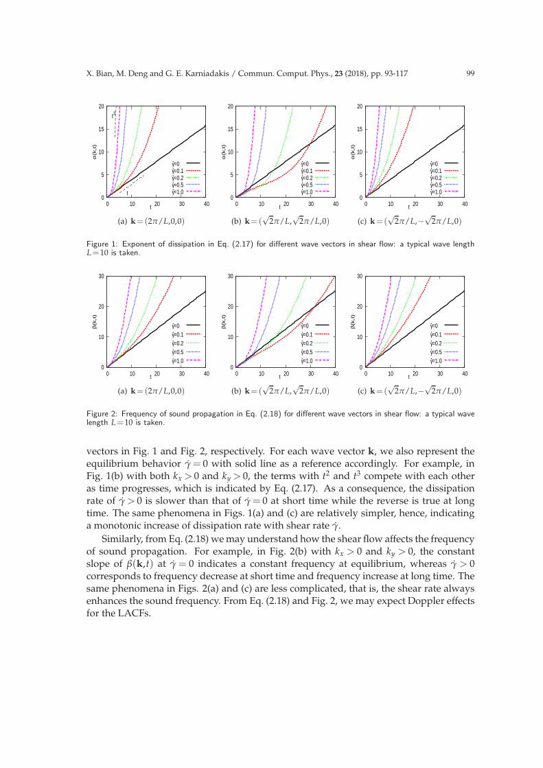
Figure 1: Exponent of dissipation in Eq. (2.17) for different wave vectors in shear flow: a typical wave lengthL=10 is taken.

0

10

20

30

0 10 20 30 40

β(k

,t)

t

•γ=0 •γ=0.1•γ=0.2•γ=0.5•γ=1.0

(a) k=(2π/L,0,0)

0

10

20

30

0 10 20 30 40

β(k

,t)

t

•γ=0 •γ=0.1•γ=0.2•γ=0.5•γ=1.0

(b) k=(√

2π/L,√

2π/L,0)

0

10

20

30

0 10 20 30 40

β(k

,t)

t

•γ=0 •γ=0.1•γ=0.2•γ=0.5•γ=1.0

(c) k=(√

2π/L,−√

2π/L,0)

Figure 2: Frequency of sound propagation in Eq. (2.18) for different wave vectors in shear flow: a typical wavelength L=10 is taken.

vectors in Fig. 1 and Fig. 2, respectively. For each wave vector k, we also represent theequilibrium behavior γ = 0 with solid line as a reference accordingly. For example, inFig. 1(b) with both kx > 0 and ky > 0, the terms with t2 and t3 compete with each otheras time progresses, which is indicated by Eq. (2.17). As a consequence, the dissipationrate of γ > 0 is slower than that of γ = 0 at short time while the reverse is true at longtime. The same phenomena in Figs. 1(a) and (c) are relatively simpler, hence, indicatinga monotonic increase of dissipation rate with shear rate γ.

Similarly, from Eq. (2.18) we may understand how the shear flow affects the frequencyof sound propagation. For example, in Fig. 2(b) with kx > 0 and ky > 0, the constantslope of β(k,t) at γ = 0 indicates a constant frequency at equilibrium, whereas γ > 0corresponds to frequency decrease at short time and frequency increase at long time. Thesame phenomena in Figs. 2(a) and (c) are less complicated, that is, the shear rate alwaysenhances the sound frequency. From Eq. (2.18) and Fig. 2, we may expect Doppler effectsfor the LACFs.


3 Dissipative particle dynamics

The method of dissipative particle dynamics (DPD) was invented two decades ago tosimulate rheological properties of complex fluids at mesoscale [30]. In this section, weshall briefly revisit the classical DPD method and its implementation of boundary condi-tions in shear flow.

3.1 Pairwise forces

For convenience, as reference we define some simple notations

rij = ri−rj,

vij =vi−vj, (3.1)

eij = rij/rij, rij = |rij|,

where ri, vi are position and velocity of particle i; rij, vij are relative position and velocityof particles i and j; rij is the distance between the two and eij is the unit vector pointing jto i. The three pairwise forces are described as follows [31, 32],

FCij = aWC(rij)eij, (3.2)

FDij =−γWD(rij)(eij ·vij)eij, (3.3)

FRij =σWR(rij)θijeijδt−1/2, (3.4)

where coefficients a, γ, and σ reflect the strength of individual forces; WC, WD, and WR

are weighting functions that monotonically decay with the relative distance rij; θij = θji isa Gaussian white noise with

< θij(t)>=0, (3.5)

< θij(t)θkl(t′)>=

(δikδjl+δilδjk

)δ(t−t′). (3.6)

The DPD version of the fluctuation-dissipation theorem reads as

WD(rij)=[WR(rij)

]2, (3.7)

2kBTγ=σ2, (3.8)

which warrants the canonical ensemble [31].Given the underlying force fields of molecular dynamics (MD), the actual forms of

the three pairwise forces may be constructed via the Mori-Zwanzig projection [33, 35].Without referring to any particular MD system, a typical empirical form of the weightingkernel is suggested as [32, 36]

WC,R(rij)=

{(1−rij/rc)k, rij < rc,

0, rij ≥ rc.(3.9)


Following [58], we take a= 25.0, σ= 3.0, γ= 4.5, rc = 1 and kBT = 1.0; k= 1 for WC andk=0.25 for WR to have a strong viscosity [41]; particle mass m=1, number density n=3.0and mass density ρ=mn= 3.0. For this particular set of input parameters, the dynamicviscosity, bulk viscosity and isothermal sound speed of the fluid are η=1.62, ζ=2.3 andcT =4.05 in DPD units [42]. The compressibility of DPD matches that of water [32]. Thevelocity Verlet time integrator is employed [32] and δt=0.005 is small enough for stability.

3.2 Boundary conditions

At nonequilibrium, the equal-time correlations of fluctuations are typically long-ranged [27] and we do not wish to introduce any extra complexities due to the boundaryeffects from the wall [60]. Therefore, we focus on the bulk behavior of the fluid in a peri-odic system, which also corresponds to the condition of the theory in Section 2. Supposethere is a simple shear flow defined as in Eq. (2.12), that is, the flow is in the x direction,the velocity gradient γ is along the y direction, and the vorticity is along the z direction.The usual periodic boundary conditions apply in the x and z directions while periodicboxes along the y direction shift ±Lyγt, above and below the principal box, respectively.Therefore, if a particle crosses y = Ly/2 to outside, it enters the principal box again aty=−Ly/2 with x shifted −Lyγt, and vx shifted by −Lyγ; if the particle crosses y=−Ly/2to outside, it enters the principal box again at y=Ly/2 with x shifted Lyγt, and vx shiftedby Lyγ. Furthermore, the x and z positions are always wrapped back into the princi-pal box due to the periodic boundaries. This is the so-called Lees-Edwards boundarycondition [12], which degenerates to the usual periodic box when γ=0.

In practice, we utilize an implementation of the deforming triclinic box for the peri-odic shear flow in the LAMMPS package [61]. In nonequilibrium MD, it is the so-calledSLLOD dynamics for the canonical ensemble [12]. The technical difference is that DPDhas a built-in pairwise thermostat while MD relies on other classical thermostats, such asthe Nose-Hoover thermostat.

4 Results

To compare the results of simulations with that of the theory, we perform DPD simula-tions in a box of [0,Lx]×[−Ly/2,Ly/2]×[0,Lz] so that the mean velocity vx = γy is con-sistent with the definition of the analytical solutions. The domain is a cube with sizeLx = Ly = Lz=10. Input parameters of DPD are given in Section 33.1. In the simulations,we define the fluctuating velocity under stationary shear flow as

δvµ(x,t)=vµ(x,t)−γδµxδσyxσ. (4.1)

The ACFs in k-space are calculated as

< δuσ(−k,t)δuσ(k,t+τ)>=1

Ns

Ns

∑s=1

< δuσ(−k,t)< δuσ(k,t+τ), (4.2)


where direction σ = 1, 2, and 3, and Ns is the number of independent simulation runs.The Fourier transform in space is defined as

δv(k,t)=1

Np

Np

∑j=1

δv(xj,t)eik(t)·xj(t), (4.3)

δuσ(k,t)= δv(k,t)·eσ, (4.4)

where j is particle index and Np is the number of particles in each simulation. Notethat fluctuating velocities are projected on unit vectors in the wave vector coordinate viaEq. (4.4) after transformed in Eq. (4.3).

At equilibrium, there is no time origin, therefore time averaging may be performedbefore ensemble averaging in Eq. (4.2) so that good statistics are obtained. At nonequi-librium, due to the time dependence of k(t), basis vectors eσ for wave vector coordinateis also time dependent (see Appendix B), and hence it is generally much more expensiveto reduce the statistical errors of ACFs. Previously we have demonstrated that when thewave k0 = (0,0,kz 6= 0) is along the vorticity direction [58], the two TACFs under shearflow degenerate to be isotropic just as that of equilibrium. Therefore, in the followingresults, we shall consider kz =0 and focus on the wave vectors within the shear plane.

4.1 Transversal autocorrelation functions: k0=(2π/Lx ,0,0)

If a wave vector along x direction as k0=(2π/Lx,0,0) is selected, the dissipation of TACFsaccording to Eq. (2.17) is

α(k,τ)= k20τ+

1

3γ2k2

xτ3. (4.5)

Therefore, it is expected that the dissipation resembles the equilibrium behavior ∼ τ atshort time while it is dominated by the advection behavior ∼τ3 at long time. The distinc-tion of two time regimes can be observed for both TACFs as shown in Fig. 3. Equilibriumresults with γ=0 are also shown as reference; with increasing shear rate γ, the dissipationrate is enhanced. We note that the two TACFs have different intercepts with the x axis, asthe extra term k0/k(τ) for CT1

(k,τ) in Eq. (2.15) causes a further stronger decay.For γ = 1.0, the condition of γ. νk2 ≈ 0.213 is violated and we can clearly see that

CT1(k,τ) of the simulations deviates from the theory of Eq. (2.15). For γ= 0.5, although

the condition of γ.νk2 is not strictly satisfied, γ can still be treated as in the order of k2

in the perturbation method. Therefore, the TACFs for γ≤0.5 from the simulations agreewith those from the theory very well.

4.2 Transversal autocorrelation functions: k0=(2π/Lx ,±2π/Ly,0)

If a wave vector is selected within the shear plane with both nonzero x and y components,the dissipation rate according to Eq. (2.17) is

α(k,τ)= k20τ−γkxkyτ2+

1

3γ2k2

xτ3. (4.6)


0.01

0.1

1

0 5 10 15 20

CT

1(k,τ

)

τ

incr

easin

g •γ

note

•γ=0

τ

τ3

0.01

0.1

1

0 5 10 15 20

CT

2(k,τ

)

τ

incr

easin

g •γ

•γ=0

τ

τ3

Figure 3: Transversal autocorrelation functions (TACFs) for k0=(2π/Lx,0,0). Left: CT1(k,t). Right: CT2

(k,t).γ= 1.0, 0.5, 0.2, 0.1 and 0 (at equilibrium). Lines are from theory and symbols are from DPD simulations.Linear scale is along the x axis and logarithmic scale is along the y axis.

0.01

0.1

1

0 5 10 15

CT

1(k,τ

)

τ

•γ=0

•γ=0.1

•γ=0.2

•γ=0.5•γ=1

note

0.01

0.1

1

0 5 10 15

CT

2(k,τ

)

τ

•γ=0

•γ=0.1

•γ=0.2

•γ=0.5•γ=1

Figure 4: Transversal autocorrelation functions (TACFs) for k0 = (2π/Lx,2π/Ly,0). Left: CT1(k,t). Right:

CT2(k,t). γ=1.0, 0.5, 0.2, and 0.1. Lines are from theory and symbols are from DPD simulations. For γ=0 at

equilibrium, only the theory is plotted in solid lines as reference. Linear scale is along the x axis and logarithmicscale is along the y axis.

If ky > 0, for example, k0 = (2π/Lx,2π/Ly,0), then the negative τ2 term competes withpositive τ and τ3 terms. Therefore, compared to the case of equilibrium, dissipation maydecrease or increase at different time regimes. This is well depicted for both CT1

(k,t) andCT2

(k,t) in Fig. 4. It is noteworthy that the discrepancy between CT1(k,t) of simulations

and that of theory at γ=1 is again apparent.

If a wave vector k0 = (2π/Lx,−2π/Ly,0) is selected, the three terms with differentpowers of τ in Eq. (4.6) are all positive. Therefore, only enhancement of dissipation isexpected compared to the case of equilibrium, which is confirmed in Fig. 5. A slightdiscrepancy is noted for CT1

(k,τ) between the simulations and the theory at γ=1.


0.01

0.1

1

0 3 6 9

CT

1(k,τ

)

τ

incre

asing

•γ

note

•γ=0

0.01

0.1

1

0 3 6 9

CT

2(k,τ

)

τ

incre

asing

•γ

•γ=0

Figure 5: Transversal autocorrelation functions (TACFs) for k0 =(2π/Lx,−2π/Ly,0). Left: CT1(k,t). Right:

CT2(k,t). γ=1.0, 0.5, 0.2, and 0.1. Lines are from theory and symbols are from DPD simulations. For γ=0 at

equilibrium, only the theory is plotted in solid lines as reference. Linear scale is along the x axis and logarithmicscale is along the y axis.

.

4.3 Longitudinal autocorrelation functions: k0=(2π/Lx ,0,0) andk0=(2π/Lx ,±2π/Ly,0)

In this section, we evaluate the LACFs from both the DPD simulations and the theory.As indicated in Eq. (2.14), the LACF has both damping and oscillating elements. Thedamping is primarily determined by the dissipation rate described by α(k,τ) functiongiven in Eq. (2.17) and much of its behavior has been seen in Sections 4.1 and 4.2. Herewe shall focus on the frequency of sound propagation, which is determined by the β(k,τ)function and it is repeated here

β(k,τ)=1

2γkx

{kyk0−ky(τ)k(τ)−k2

⊥ In

[ky(τ)+k(τ)

ky+k0

]}. (4.7)

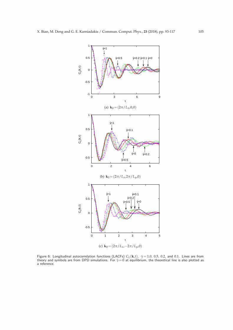
When the wave vector is k0 =(2π/Lx,0,0) along x direction, the sound frequency is ex-pected to increase monotonically with shear rate γ, as already indicated in Fig. 2(a). Wefurther show the LACFs of both DPD simulations and the theory for this wave vector inFig. 6(a). We clearly observe an overall agreement between the results of DPD simulationand the theory, and the sound frequency indeed increases monotonically with γ. A smalldiscrepancy between the simulation and the theory is observed for γ=1.

When the wave vector is k0=(2π/Lx,2π/Ly,0), it is already suggested in Fig. 2(b) thatthe sound frequency may increase or decrease at different time regimes. This is explicitlyconfirmed by the LACFs of both DPD simulations and the theory as shown in Fig. 6(b).We may observe that simulations agree with the theory at all shear rates considered.

When the wave vector is k0 = (2π/Lx,−2π/Ly,0), it is known from Fig. 2(c) thatsound frequency increases with γ. Again this can be observed in the LACFs in Fig. 6(c),where the results of the simulations agree with the theory at all shear rates considered.


-1

-0.5

0

0.5

1

0 3 6 9

CL(

k,τ)

τ

•γ=0•γ=0.1•γ=0.2•γ=0.5

•γ=1

(a) k0=(2π/Lx,0,0)

-0.5

0

0.5

1

0 2 4 6

CL(

k,τ)

τ

•γ=0

•γ=0.1

•γ=0.2

•γ=0.5

•γ=1

(b) k0=(2π/Lx,2π/Ly,0)

-0.5

0

0.5

1

0 1 2 3 4 5

CL(

k,τ)

τ

•γ=0

•γ=0.1•γ=0.2

•γ=0.5

•γ=1

(c) k0 =(2π/Lx,−2π/Ly,0)

Figure 6: Longitudinal autocorrelation functions (LACFs) CL(k,t). γ= 1.0, 0.5, 0.2, and 0.1. Lines are fromtheory and symbols are from DPD simulations. For γ=0 at equilibrium, the theoretical line is also plotted asa reference.


4.4 Small length scales at γ=1

Here we revisit various ACFs at γ=1, where some discrepancies between the simulationsand the theory have been observed for the largest length scale or smallest wave numberconsidered. For those cases, the condition γ. νk2 is not met. Instead, here we focus onwave vectors k0=(2nwπ/Lx,0,0) and k0=(2nwπ/Lx,±2nwπ/Ly,0), but with nw=2 or 3.Therefore, the condition γ.νk2 becomes valid again for the smaller length scales and weexpect that the perturbation method in deriving the analytical solutions is accurate. Thiscan be confirmed by the TACFs CT1

(k,t) for different wave vectors with nw =2 and 3, asshown in Fig. 7. The same results of nw=1 as in Figs. 3(a), 4(a) and 5(a) are plotted againin Fig. 7 for comparison.

Similarly for the LACFs at nw = 2 and 3, results of the simulations agree well withthose of the theory, since the condition γ . νk2 is valid, as shown in Fig. 8. The sameresults of nw =1 as in Fig. 6 are shown again in Fig. 8 for comparison.

It is noteworthy that at an even smaller scale (nw > 3), another type of discrepancybetween the simulations and the theory emerges. This is due to the fact that the classicalfluctuating hydrodynamics may not describe well the collective behavior of the DPD sim-ulations at this small scales [43, 45]. In this case, solutions of the generalized fluctuatinghydrodynamics may be required [9], which is beyond the scope of the current work.

5 Discussion and summary

We studied the autocorrelations (ACFs) of hydrodynamic fluctuations in k-space for anisothermal fluid under shear flow, which is driven by the Lees-Edwards periodic bound-ary condition. We compared results of the ACFs from the dissipative particle dynamics(DPD) simulations with the theoretical approximations. DPD is a particle-based meso-scopic method with three pairwise forces between neighboring particles. After specify-ing the conservative, dissipative and random forces, DPD is an effective simulator forthe compressible fluctuating hydrodynamics. Under the assumption of a local thermo-dynamic equilibrium, the dissipative and random forces act as an intrinsic thermostatand they satisfy the fluctuation-dissipation theorem. In principle, the DPD method isvalid for an arbitrarily large shear rate γ, so are its ACFs of fluctuations, as long as localthermodynamic equilibrium is valid.

In order to derive the analytical solutions for the various ACFs, a perturbationmethod is adopted to expand the eigenvalue and eigenvector as a power series of k,where the parameter k is the inverse of wave-length and it is very small in the hydrody-namic limit. In such regime, νk2≪cTk holds so that the rate of hydrodynamic dissipationis much smaller than the rate of sound propagation. Here ν and cT are the kinematicviscosity and isothermal sound speed, respectively. In the perturbation method, it is as-sumed that γ.νk2. Therefore, terms of γ are treated as in the order of k2. With such anassumption, the generalized eigenvalue problem was solved approximately and there-after the longitudinal and the two transversal ACFs were constructed as in Eqs. (2.14),


0.01

0.1

1

0 1 2 3 4

CT

1(k,τ

)

τ

incre

asing

|k|

•γ=0

•γ=0

•γ=0

(a) k0=(2nwπ/Lx,0,0)

0.01

0.1

1

0 1 2 3 4 5

CT

1(k,τ

)

τ

increasin

g |k|

•γ=0

•γ=0

•γ=0

(b) k0=(2nwπ/Lx,2nwπ/Ly,0)

0.01

0.1

1

0 1 2 3

CT

1(k,τ

)

τ

increasin

g |k|

•γ=0

•γ=0

•γ=0

(c) k0 =(2nwπ/Lx,−2nwπ/Ly,0)

Figure 7: Transversal autocorrelation functions (TACFs) CT1(k,t) at γ = 1: Wave number nw = 1,2, and 3.

Lines are from theory and symbols are from DPD simulations. The theoretical results for γ=0 at equilibriumare also plotted in solid lines for reference. Results of nw =1 are the same as in Figs. 3(a), 4(a), and 5(a).


-1

-0.5

0

0.5

1

0 1 2 3

CL(

k,τ)

τ

nw=1

nw=2nw=3

(a) k0=(2nwπ/Lx,0,0)

-0.5

0

0.5

1

0 1 2 3

CL(

k,τ)

τ

nw=1

nw=2nw=3

(b) k0=(2nwπ/Lx,2nwπ/Ly,0)

-0.5

0

0.5

1

0 0.5 1 1.5 2

CL(

k,τ)

τ

nw=1

nw=2nw=3

(c) k0=(2nwπ/Lx,−2nwπ/Ly,0)

Figure 8: Longitudinal autocorrelation functions (LACFs) CL(k,t) at γ= 1: Wave number nw = 1,2, and 3.Lines are from theory and symbols are from DPD simulations. Results of nw=1 are the same as in Fig. 6.


(2.15), and (2.16).

When the condition of γ . νk2 is met, that is, Reynolds number Re = γL2/ν . 4π2,various ACFs of the analytical solutions are accurate and agree very well with thoseof DPD simulations. We observed that the two transversal ACFs in shear flow are nolonger identical as in equilibrium and the dissipation rate is time dependent as well.Furthermore, depending on the individual wave vector k, enhancement or attenuationof sound frequency may take place and we observed the Doppler effects. Given theincreasing efforts on hybrid modeling of fluid flow, where usually a stochastic micro-scopic/mesoscopic solver is concurrently coupled with a continuum (Landau-Lifshitz-)Navier-Stokes solver [53, 58], the agreement between analytical and computational ap-proaches on the results is meaningful: the temporal correlations of fluctuating variablesprovide a fundamental benchmark for any proposed coupling algorithm.

When νk2< γ< cTk, some discrepancies between the ACFs of the analytical solutions

and those of the DPD simulations are observed. In this regime, besides the couplingbetween the advection and fluctuating variables, extra couplings between different fluc-tuating variables at equal time are expected to be significant. In our DPD simulationsthese extra couplings affect significantly both CT1

and CL, but have a negligible effecton CT2

. In this regime of shear rates, the perturbation theory is inaccurate and shouldbe modified to treat the terms of γ as in the order of k instead of k2. Furthermore, thecontributions from the stochastic stress on the temporal correlations are also expected toemerge. However, such modifications on the theory are nontrivial to accomplish and aresubjects of our future research. Nevertheless, the DPD simulations are in principle validand provide a few guidelines on how to improve the theory. In this regime, compari-son with results from other numerical methods such as the finite volume method withthermal fluctuations [62, 63] would also be helpful to confirm the results presented.

When the shear rate becomes even larger such as γ>cTk, we obtain a nonequilibriumstate far from equilibrium and additional couplings between different k are expected (re-sults are not shown). The local thermodynamic equilibrium is produced and enforcedby the frequent collisions between particles and the frequency is measured by the soundspeed cT divided by the length scale, that is cTk. Therefore, under such strong shear flowthe local thermodynamic equilibrium can no longer be restored in the length scale of 1/k.It would also be interesting to evaluate the probability of violating the Second law in sucha DPD system.

Acknowledgments

This work was supported by the Computational Mathematics Program within the De-partment of Energy office of Advanced Scientific Computing Research as part of theCollaboratory on Mathematics for Mesoscopic Modeling of Materials (CM4) and alsosupported by the ARO grant W911NF-14-1-0425. Part of this research was conductedusing computational resources and services at the Center for Computation and Visual-


ization, Brown University. An award of computer time was provided by the Innovativeand Novel Computational Impact on Theory and Experiment (INCITE) program. Thisresearch used resources of the Argonne Leadership Computing Facility, which is a DOEOffice of Science User Facility supported under contract DE-AC02-06CH11357. This re-search also used resources of the Oak Ridge Leadership Computing Facility, which is aDOE Office of Science User Facility supported under Contract DE-AC05-00OR22725. X.B. acknowledges discussions with Dr. Fanhai Zeng on the generalized eigenvalue prob-lem.

Appendices

A Linearization around uniform shear flow

The fluctuations on the state variables are defined as

z(x,t)= [δρ(x,t),δv(x,t)], (A.1)

with

δρ=ρ−ρ0 =ρ−<ρ>, (A.2)

δv=v−v0=v−<v>, (A.3)

where the macroscopic state variables are the averaged quantities denoted by “< >”.Therefore, the fluctuating hydrodynamic equations can be linearized as

(∂

∂t+γµσxσ

∂

∂xµ

)δρ+ρ0∇·δv=0, (A.4)

(∂

∂t+γµσxσ

∂

∂xµ

)δvµ+γµσδvσ+

c2T

ρ0

∂

∂xµδρ

−ν∇2δvµ−(

κ+ν

3

) ∂

∂xµ∇·δv=

1

ρ0

∂

∂xµΠR

µσ, (A.5)

where second-order terms in fluctuations are neglected. Kinematic viscosities are definedas ν = η/ρ0 and κ = ζ/ρ0. Furthermore, the equation of state is assumed to have theproperty of δp= c2

Tδρ, where cT is the isothermal sound speed.

B Hydrodynamic matrix

It proves to be convenient to solve such a linearized hydrodynamic equations ofEqs. (A.4) and (A.5) in Fourier space [1,8,9]. Hence, we define the fluctuations in k-spaceas the spatial Fourier transform of the fluctuations

z(k,t)=∫

z(x,t)eik·xdx. (B.1)


Suppose that the wave vector is defined as k= kxex+kyey+kzez =(kx,ky,kz), where ex,ey and ez are three basis vectors in the fixed Cartesian coordinate. The formulation of theproblem is very succinct, if the transformed velocity is decomposed into one componentparallel to k and the other two components perpendicular to k [26, 27]. Therefore, wedefine another three orthonormal vectors e1, e2 and e3 in such way that e1 is along k ande2,3 are perpendicular to k,

e1 =k/k, (B.2)

e2 =[ey−(e1 ·ey)e

1]

/k⊥, (B.3)

e3 =e1×e2. (B.4)

Here ey is taken as reference to define the first transversal direction e2 so that e2 is in thesame plane with e1 and ey, and e2 is perpendicular to e1; moreover, e3 is perpendicular to

both e1 and e2. Also k=|k|, k⊥=(k2−k2y)

1/2/k. Note that superscript 1, 2, or 3 refers to thepairwise orthonormal basis vectors in the wave vector coordinate or oblique coordinate,which are expressed in the fixed Cartesian coordinate.

We further define a vector of fluctuating variables in k-space as

z(k,t)=[

δρ(k,t), δu1(k,t), δu2(k,t), δu3(k,t)]

, (B.5)

where each element is related to the Fourier-transformed variable as

δρ(k,t)= cT δρ(k,t)/ρ0, (B.6)

δuµ(k,t)= δv(k,t)·eµ. (B.7)

The fluctuating velocity δv(k,t) in k-space is the spatial Fourier transform of the fluctuat-ing velocity δv(x,t) in real space. The latter is the peculiar or fluctuating velocity aroundthe macroscopic velocity field defined as

δvµ(x,t)=vµ(x,t)−γδµxδσyxσ. (B.8)

It is also simple to see that δu(k,t) is obtained by projecting δv(k,t) onto the basis direc-

tions of the wave vector. Hence, δu1(k,t) is called the longitudinal fluctuating compo-

nent, while δu2(k,t) and δu3(k,t) are the first and second transversal fluctuating compo-nents, respectively. Finally, the hydrodynamic equations in k-space are summarized in acompact form as

(∂

∂t−γµσkµ

∂

∂kσ

)zǫ(k,t)+Lǫι(k,γ,t)zι(k,t)= Rǫ(k,t), (B.9)

where the matrix L is defined as

L=−ikA+k2B+γC, (B.10)


with

A=

0 cT 0 0cT 0 0 00 0 0 00 0 0 0

, (B.11)

B=

0 0 0 00 νL 0 00 0 ν 00 0 0 ν

, (B.12)

C=

0 0 0 00 Φ11 Φ12 Φ13

0 Φ21 Φ22 Φ23

0 Φ31 Φ32 Φ33

. (B.13)

The longitudinal viscosity is defined as νL =4ν/3+κ=(4η/3+ζ)/ρ0 . Φµσ is defined by

γΦµσ=eµǫ (k)γǫιe

σι (k)−γǫιkǫe

µχ(k)

∂

∂kιeσ

χ(k). (B.14)

Given the definitions of the basis vectors from Eqs. (B.2), (B.3), and (B.4) in oblique coor-dinate, the elements of C read

Φ11=−Φ22 = kxky/k2, (B.15)

Φ12=−kx/k⊥, (B.16)

Φ31=−kykz/kk⊥ , (B.17)

Φ32=−kz/k, (B.18)

Φij =0, all others. (B.19)

The linear mode coupling is represented by the derivatives with respect to k.Finally, the stochastic terms are

Rǫ(k,t)= Rǫ(k,t)−< Rǫ(k,t)>, (B.20)

R1(k,t)=0, (B.21)

R2(k,t)=e1µ(k)ikσΠR

µσ(k,t)/ρ0, (B.22)


µσ(k,t)/ρ0, (B.23)


µσ(k,t)/ρ0. (B.24)

The general solution to the linearized hydrodynamic equation (Eq. (B.9)) can be de-termined from the nonlinear eigenvalue problem,

(−γµσkµ

∂

∂kσ+L

)ξ(µ)=λµξ(µ). (B.25)


The left eigenvectors χ(µ) are defined as(

χ(µ),ξ(σ))= χ

(µ)ǫ ξ

(σ)ǫ =δµσ, (B.26)

where χ(µ)ǫ means conjugate of χ

(µ)ǫ , and δµσ is the Kronecker δ

The eigenvalues λµ and eigenvectors ξ(µ) can be obtained via the perturbation theoryby the expansion of k to second and first order, respectively

λµ = kλµ,1+k2λµ,2+··· , (B.27)

ξ(µ)= ξ(µ)0 +kξ

(µ)1 +··· . (B.28)

Inserting Eqs. (B.27) and (B.28) into Eq. (B.9) and making use of the explicit form of Lin Eq. (B.10), we have the first-order perturbation theory involving A and second-orderperturbation theory involving A, B, and C all together. Assuming γ . νk2 ≪ cTk andtreating γ as in the order of k2, the two equations from the perturbation read [26, 59]

(−iA−λµ,1I

)ξ(µ)0 =0, (B.29)

(−iA−λµ,1I

)ξ(µ)1 =

(λµ,2I−B−γk−2C+k2γµσkµ

∂

∂kσ

)ξ(µ)0 . (B.30)

From Eq. (B.29), we find the first set of eigenvalues as follows

λ1,1=−icT, (B.31)

λ2,1=+icT, (B.32)

λ3,1=λ4,1=0. (B.33)

From Eq. (B.30), we find the second set of eigenvalues as follows

λ1,2==ΓT+1

2γk−2Φ11 =ΓT+

1

2γkxky/k4, (B.34)

λ2,2=λ1,1 (B.35)

λ3,2=ν+γk−2Φ22 =ν−γkxky/k4, (B.36)

λ4,2=ν, (B.37)

where sound attenuation coefficient ΓT =νL/2=(2η/3+ζ/2)/ρ0 .Inserting the expressions for λµ,1 and λµ,2 back into Eq. (B.27), finally the eigenvalues

are summarized as

λ1=−icTk+ΓTk2+1

2γkxky/k2, (B.38)

λ2=+icTk+ΓTk2+1

2γkxky/k2, (B.39)

λ3=νk2−γkxky/k2, (B.40)

λ4=νk2. (B.41)


Furthermore, the corresponding right eigenvectors are

ξ(1)=1√2(1,1,0,0)T , (B.42)

ξ(2)=1√2(0,0,0,1)T , (B.43)

ξ(3)=(0,0,1,M)T , (B.44)

ξ(4)=(0,0,0,1)T , (B.45)

where

M(k)=kkz

kxk⊥arctan

( ky

k⊥

), (B.46)

k⊥= k2−k2y. (B.47)

The corresponding left eigenvectors satisfying Eq. (B.26) are

χ(1)=1√2(1,1,0,0)T , (B.48)

χ(2)=1√2(0,0,0,1)T , (B.49)

χ(3)=(0,0,1,0)T , (B.50)

χ(4)=(0,0,−M,1)T . (B.51)

Given the eigenvalues and eigenvectors λµ, ξµ and χµ, the time evolution of fluctuat-ing variables is obtained as

zǫ(k(t),t)=4

∑ι=1

Gǫι(k(t),t)zι(k,0)+∫ t

0

4

∑ι=1

Gǫι(k(t−u),t−u)Rι(k,u)du, (B.52)

with a propagator defined as

Gǫι(k(t),t)=4

∑µ=1

ξ(µ)ǫ (k(t))χ

(µ)ι (k)e−

∫ t0 dτλµ(k(τ)). (B.53)

To account for the advection, the wave vector is time dependent k(t)= (kx,ky−γtkx,kz).Since the random terms do not contribute in this shear rate regime [26, 29], the correla-tions of the fluctuating variables are readily expressed as

Cǫι(k,−k,t)=< zǫ(k(t),t)zι(−k,0)>=4

∑µ=1

Gǫµ(k(t),t)< zµ(k,0)zι(−k,0)> . (B.54)

Given the values of λµ, ξµ and χµ,, we find that Gǫι=0 for ǫ 6= ι and Gǫι 6=0 for ǫ= ι.


References

[1] J. P. Hansen and I. R. McDonald. Theory of simple liquids. Elsevier, 4 edition, 2013.[2] G. E. Karniadakis, A. Beskok, and N. Aluru. Microflows and nanoflows: fundamentals and

simulation. Springer, New York, 2005.[3] J. Mewis and N. J. Wagner. Colloidal suspension rheology. Cambridge University Press, Cam-

bridge, 2012.[4] X. Li, Z. Peng, H. Lei, M. Dao, and G. E. Karniadakis. Probing red blood cell mechanics,

rheology and dynamics with a two-component multi-scale model. Phil. Trans. R. Soc. A,372(2021), 2014.

[5] H. M. Jaeger, S. R. Nagel, and R. P. Behringer. Granular solids, liquids, and gases. Rev. Mod.Phys., 68:1259–1273, Oct 1996.

[6] V. Springel. Smoothed particle hydrodynamics in astrophysics. Annu. Rev. Astron. Astrophys.,48:391–430, 2010.

[7] R. Kubo. The fluctuation-dissipation theorem. Rep. Prog. Phys., 29(1):255, 1966.[8] L. P. Kadanoff and P. C. Martin. Hydrodynamic equations and correlation functions. Ann.

Phys., 24:419 – 469, 1963.[9] J. P. Boon and S. Yip. Molecular hydrodynamics. Dover Publications, Inc., New York, 1991.

[10] X. Bian, C. Kim, and G. E. Karniadakis. 111 years of Brownian motion. Soft Matter, 12:6331–6346, 2016.

[11] D. J. Evans, E. G. D. Cohen, and G. P. Morriss. Probability of second law violations inshearing steady states. Phys. Rev. Lett., 71:2401–2404, 1993.

[12] D. J. Evans and G. Morriss. Statistical mechanics of nonequilibrium liquids. Cambridge Univer-sity Press, second edition, 2008.

[13] U. Seifert. Stochastic thermodynamics, fluctuation theorems and molecular machines. Rep.Prog. Phys., 75(12):126001, 2012.

[14] L. Bertini, A. De Sole, D. Gabrielli, G. Jona-Lasinio, and C. Landim. Macroscopic fluctuationtheory. Rev. Mod. Phys., 87:593–636, Jun 2015.

[15] U. M. B. Marconi, A. Puglisi, L. Rondoni, and A. Vulpiani. Fluctuation-dissipation: responsetheory in statistical physics. Phy. Rep., 461(4-6):111–195, 2008.

[16] J. Machta, I. Oppenheim, and I. Procaccia. Statistical mechanics of stationary states. v. fluc-tuations in systems with shear flow. Phys. Rev. A, 22:2809–2817, Dec 1980.

[17] A. M. S. Tremblay, M. Arai, and E. D. Siggia. Fluctuations about simple nonequilibriumsteady states. Phys. Rev. A, 23:1451–1480, Mar 1981.

[18] A. L. Garcia, M. Malek Mansour, G. C. Lie, M. Mareschal, and E. Clementi. Hydrodynamicfluctuations in a dilute gas under shear. Phys. Rev. A, 36:4348–4355, Nov 1987.

[19] M. Malek Mansour, John W. Turner, and Alejandro L. Garcia. Correlation functions for sim-ple fluids in a finite system under nonequilibrium constraints. Journal of Statistical Physics,48(5):1157–1186, 1987.

[20] B. F. Farrell and P. J. Ioannou. Stochastic forcing of the linearized navierstokes equations.Physics of Fluids A: Fluid Dynamics, 5(11):2600–2609, 1993.

[21] H. Wada. Shear-induced quench of long-range correlations in a liquid mixture. Phys. Rev. E,69:031202, Mar 2004.

[22] J. M. Ortiz de Zarate and J. V. Sengers. Transverse-velocity fluctuations in a liquid understeady shear. Phys. Rev. E, 77:026306, Feb 2008.

[23] J. M. Ortiz de Zarate and J. V. Sengers. Nonequilibrium velocity fluctuations and energyamplification in planar couette flow. Phys. Rev. E, 79:046308, Apr 2009.


[24] Jun Zhang and Jing Fan. Monte carlo simulation of thermal fluctuations below the onset ofrayleigh-benard convection. Phys. Rev. E, 79:056302, May 2009.

[25] J. M. Ortiz de Zarate and J. V. Sengers. Hydrodynamic fluctuations in laminar fluid flow. i.fluctuating orr-sommerfeld equation. J. Stat. Phys., 144(4):774–792, 2011.

[26] J. Lutsko and J. W. Dufty. Hydrodynamic fluctuations at large shear rate. Phys. Rev. A,32:3040–3054, Nov 1985.

[27] M. Otsuki and H. Hayakawa. Spatial correlations in sheared isothermal liquids: from elasticparticles to granular particles. Phys. Rev. E, 79:021502, Feb 2009.

[28] M. Otsuki and H. Hayakawa. Long-time tails for sheared fluids. J. Stat. Phys.: Theor. Exp.,2009(08):L08003, 2009.

[29] A. Varghese, C. Huang, R. G. Winkler, and G. Gompper. Hydrodynamic correlations in shearflow: multiparticle-collision-dynamics simulation study. Phys. Rev. E, 92:053002, Nov 2015.

[30] P. J. Hoogerbrugge and J. M. V. A. Koelman. Simulating microsopic hydrodynamics phe-nomena with dissipative particle dynamics. Europhys. Lett., 19(3):155–160, 1992.

[31] P. Espanol and P. Warren. Statistical mechanics of dissipative particle dynamics. Europhys.Lett., 30(4):191–196, May 1995.

[32] R. D. Groot and P. B. Warren. Dissipative particle dynamics: Bridging the gap betweenatomistic and mesoscopic simulation. J. Chem. Phys., 107(11):4423–4435, 1997.

[33] C. Hijon, P. Espanol, E. Vanden-Eijnden, and R. Delgado-Buscalioni. Mori-Zwanzig formal-ism as a practical computational tool. Farad. Discuss., 144:301–322, 2010.

[34] H. Lei, B. Caswell, and G. E. Karniadakis. Direct construction of mesoscopic models frommicroscopic simulations. Phy. Rev. E, 81:026704, 2010.

[35] Z. Li, X. Bian, B. Caswell, and G. E. Karniadakis. Construction of dissipative particle dynam-ics models for complex fluids via the Mori-Zwanzig formulation. Soft Matter, 10:8659–8672,2014.

[36] X. Fan, N. Phan-Thien, N. T. Yong, X. Wu, and D. Xu. Microchannel flow of a macromolec-ular suspension. Phys. Fluids, 15:11–21, 2003.

[37] Z. Li, X. Bian, X. Yang, and G. E. Karniadakis. A comparative study of coarse-grainingmethods for polymeric fluids: Mori-Zwanzig vs. iterative Boltzmann inversion vs. stochasticparametric optimization. J. Chem. Phys., 145(4), 2016.

[38] C. A. Marsh, G. Backx, and M. H. Ernst. Static and dynamic properties of dissipative particledynamics. Phys. Rev. E, 56:1676–1691, Aug 1997.

[39] J. A. Backer, C. P. Lowe, H. C. J. Hoefsloot, and P. D. Iedema. Poiseuille flow to measure theviscosity of particle model fluids. J. Chem. Phys., 122:154503, 2005.

[40] D. A. Fedosov, G. E. Karniadakis, and B. Caswell. Steady shear rheometry of dissipative par-ticle dynamics models of polymer fluids in reverse Poiseuille flow. J. Chem. Phys., 132:144103,2010.

[41] H. Lei, D. A. Fedosov, and G. E. Karniadakis. Time-dependent and outflow boundary con-ditions for dissipative particle dynamics. J. Comput. Phys., 230:3765–3779, 2011.

[42] X. Bian, Z. Li, M. Deng, and G. E. Karniadakis. Fluctuating hydrodynamics in periodicdomains and heterogeneous adjacent multidomains: Thermal equilibrium. Phys. Rev. E,92:053302, Nov 2015.

[43] D. Azarnykh, S. Litvinov, X. Bian, and N. A. Adams. Determination of macroscopic transportcoefficients of DPD solvent. Phys. Rev. E, 93:013302, 2016.

[44] L. D. Landau and E. M. Lifshitz. Fluid mechanics, volume 6 of Course of theoretical physics.Pergamon Press, Oxford, 1959.

[45] M. Ripoll, M. H. Ernst, and P. Espanol. Large scale and mesoscopic hydrodynamics for


dissipative particle dynamics. J. Chem. Phys., 115:7271–7284, 2001.[46] Z. Li, X. Bian, X. Li, and G. E. Karniadakis. Incorporation of memory effects in coarse-

grained modeling via the Mori-Zwanzig formalism. J. Chem. Phys., 143(24):243128, 2015.[47] H. Lei, N. A. Baker, and X. Li. Data-driven parameterization of the generalized langevin

equation. Proc. Nat. Acad. Sci., 113(50):14183–14188, 2016.[48] Z. Li, H. S. Lee, E. Darve, and G. E. Karniadakis. Computing the non-Markovian coarse-

grained interactions derived from the MoriZwanzig formalism in molecular systems: Ap-plication to polymer melts. J. Chem. Phys., 146(1):014104, 2017.

[49] W. Pan, B. Caswell, and G. E. Karniadakis. Rheology, microstructure and migration in Brow-nian colloidal suspensions. Langmuir, 26(1):133–142, 2009.

[50] X. Bian, S. Litvinov, R. Qian, M. Ellero, and N. A. Adams. Multiscale modeling of particle insuspension with smoothed dissipative particle dynamics. Phys. Fluids, 24(1):012002, 2012.

[51] W. E, B. Engquist, X. Li, W. Ren, and E. Vanden-Eijnden. Heterogeneous multiscale method:A review. Commun. Comput. Phys., 2(3):367–450, 2007.

[52] M. Praprotnik, L Delle Site, and K. Kremer. Multiscale simulation of soft matter: from scalebridging to adaptive resolution. Annu. Rev. Phys. Chem., 59:545–571, 2008.

[53] R. Delgado-Buscalioni. Tools for multiscale simulation of liquids using open molecular dy-namics. In B. Engquist, O. Runborg, and Y.-H. R. Tsai, editors, Numerical analysis of multiscalecomputations, volume 82 of Lecture Notes in Computational Science and Engineering, pages 145–166. Springer Berlin Heidelberg, 2012.

[54] M. K. Borg, D. A. Lockerby, and J. M. Reese. A hybrid molecular-continuum method forunsteady compressible multiscale flows. J. Fluid Mech., 768:388–414, 4 2015.

[55] X. Bian, Z. Li, and G. E. Karniadakis. Multi-resolution flow simulations by smoothed particlehydrodynamics via domain decomposition. J. Comput. Phys., 297(0):132 – 155, 2015.

[56] Y.-H. Tang, S. Kudo, X. Bian, Z. Li, and G. E. Karniadakis. Multiscale universal interface: Aconcurrent framework for coupling heterogeneous solvers. J. Comput. Phys., 297:13–31, 2015.

[57] P. Perdikaris, D. Venturi, J. O. Royset, and G. E. Karniadakis. Multi-fidelity modelling viarecursive co-kriging and Gaussian-Markov random fields. Proc. R. Soc. A, 471(2179), 2015.

[58] X. Bian, M. Deng, Y.-H. Tang, and G. E. Karniadakis. Analysis of hydrodynamic fluctuationsin heterogeneous adjacent multidomains in shear flow. Phys. Rev. E, 93:033312, 2016.

[59] J. F. Lutsko. Nonequilibrium fluctuations and transport in shear fluids. PhD thesis, University ofFlorida, 1986.

[60] J. M. Ortiz de Zarate and J. V. Sengers. Hydrodynamic fluctuations in laminar fluid flow. ii.fluctuating squire equation. J. Stat. Phys., 150(3):540–558, 2013.

[61] S. Plimpton. Fast parallel algorithms for short-range molecular dynamics. J. Comput. Phys.,117(1):1 – 19, 1995.

[62] G. De Fabritiis, M. Serrano, R. Delgado-Buscalioni, and P. V. Coveney. Fluctuating hydrody-namic modeling of fluids at the nanoscale. Phys. Rev. E, 75:026307, Feb 2007.

[63] A. Chaudhri, J. B. Bell, A. L. Garcia, and A. Donev. Modeling multiphase flow using fluctu-ating hydrodynamics. Phys. Rev. E, 90:033014, Sep 2014.

AnalyticalandComputationalStudiesofCorrelations of ... ·...

Documents

Transcript of AnalyticalandComputationalStudiesofCorrelations of ... ·...