Analytical Research Series - INSEADfaculty.insead.edu/joel-peress/documents/dynamics... ·...

Lehman Brothers International (Europe)

INTERNATIONAL FIXED INCOME RESEARCH

Analytical Research Series

Pub Code 403

October 1999

Jamil Baz, David Mendez-Vives,David Munves, Vasant Naik and

Joel Peress

DYNAMICS OF SWAP SPREADS:A CROSS-COUNTRY STUDY

2

Analytical Research Series October 1999

Lehman Brothers International (Europe)

We examine the empirical behaviour of swap spreads in Germany, Britainand the US over the last five years. Swap spreads of three maturities (2-, 5-and 10-year) are considered. The movements of swap spreads are explainedusing the movements in credit spreads, Libor-gc spreads, the shape of thegovernment curve and returns on equity market indices. We documentevidence for a regime shift in the dynamics of swap spreads over the last 12-15 months. The level and persistence of spreads and the volatility of changesin spreads are markedly higher now.

Moreover, their sensitivity to credit spreads and the cross-country correlationin spread changes have increased significantly. An increase in investor anddealer risk aversion, the reduction in leverage of risk capital employed byrelative-value hedge funds (which were typical receivers on swaps), a percep-tion of increased risk in asset markets and increases in spread volatility inducedby lower liquidity could be cited as factors that have contributed to the recentspread widening.

Euro-area swap spreads continue to remain at half the levels of their Britishand US counterparts. Lower credit spreads in Europe and lower Libor-gcspreads may partly explain this feature. The level of issuance of credit bondsin Europe, the risk appetite of dealers and hedge funds, the shrinking supplyof Treasury securities in the US, the performance of global (especially US)equity markets and cyclical movements in the US economy relative to theEuropean economy are likely to be the key drivers of swap spreads in thenear-to-intermediate term.

Jamil [email protected]+44 –(207) 260 2602David [email protected]+44 (207) 260 1634David [email protected]+44 (207) 260 2787Vasant [email protected]+44 (207) 260 2813Joel Peress

Summary

Acknowledgements The authors would like to thank Kasper Christoffersen, Joyce Kwong, Ravi Mattu,Andy Morton, Michal Oulik, David Prieul, Stefano Risa, Arran Rowsell, ThomasSiegmund, Vikrant Singal, Stuart Sparks and Stephane Vanadia for their comments,explanations, suggestions and assistance.


Lehman Brothers International (Europe) 3

I Introduction Few sectors of the financial market have undergone a faster rate of growth andchange over the last 15 years than the interest rate swap market. Swaps werefirst used in the mid-1980s as straightforward liability management tools, withmarket participants swapping fixed for floating rate interest streams. By 1990the notional outstanding amount of swaps had grown to $2.3 trillion, but theirrange of application was limited.

In this decade developments include the creation of a new asset class, assetswaps (fixed rate bonds swapped to floating rate for bank and other Libor-based investors) and swaptions (options on forward swaps). These instru-ments allow investors to take a view on future interest rate and yield curvemovements.

The use of swaps has also expanded. Hedge funds use swaps both to takeviews on credit spread direction and to profit from price movements in therepo market. Bond dealers are increasingly using swaps to hedge cash posi-tions. The notional amount of swaps outstanding is now over $50 trillion.The rate of growth has far outstripped that of any other financial market.Daily turnover in the swap market, estimated at about $5bn in 1990 is nowclose to $150bn.

Financial markets are interrelated, and swaps lie at the centre of many mar-ket relationships. Swap markets link government, corporate debt and moneymarkets across currencies (via basis swaps) and maturities. So, the variablesthat drive the underlying term structure of the government and credit curvesshould explain swap spread movements. At the same time, the dynamics ofswap spreads should be helpful in understanding bond markets. These con-siderations underline that a range of factors needs to be analysed in order tounderstand movements in swap spreads. Moreover, the importance of eachfactor, along with their interrelationships, most likely changes over time.

This study documents empirically the linkages between swap, government creditand volatility markets. We construct a model to enable us to assess quantitativelywhether movements in swap spreads are warranted by price changes in thesemarkets. This model can help investors determine the appropriate time to go longor short swap spreads. It could also be used by corporations, agencies and sover-eigns in timing debt issuance and in deciding whether or not to swap a particularissue.

This study also highlights international differences in the behaviour of swapspreads. We consider three countries — the US, Germany and the UK.Within each, we examine three maturities (2-, 5-year and 10-year). Our re-sults can provide useful inputs into decisions about international swap arbi-trages and cross-border issuance.

Our key findings on the drivers of swap spreads are as follows:

� Among the factors that help explain movements in swap spreads, the mostimportant are: credit spreads, the level of interest rates and the slope of theyield curve, and volatility and risk aversion in asset markets.

� There is evidence of a regime shift in the distribution of swap spreads sincethe financial crisis of autumn 1998. Swap spreads are now fluctuatingaround a higher mean and the volatility of spread movements is alsohigher. The sensitivity of swap spreads to credit spreads has also increasedsignificantly.


4 Lehman Brothers International (Europe)

� The reduction in risk capital devoted to relative-value trades that involvedshorting Treasuries against (receiver) swaps, the increasing specialness ofon-the-run Treasuries in the US market and perceptions of increased riskhave all contributed to spread widening. In the near-to-intermediate term,many of these factors are likely to persist and swap spreads could well re-main wider than their historical means.

� Euro swap spreads remain at half the level of their US and UK counter-parts. Lower credit and Libor-gc spreads (which in turn could be the resultof bank deposits being the dominant avenue for short-term investing inEurope, the somewhat higher credit quality of European banks and a dearthof European credit bonds) may partly explain this feature.

� Swap spreads show a mean-reversion tendency. This is stronger in the USand Germany than in the UK. The relative illiquidity of the UK market is areason for this feature.

� The correlation of swap spreads among countries has increased. In com-mon with many financial markets, it is especially high during volatile peri-ods.

This article has six sections. The next part provides a basic introduction toswap cash flows and the valuation of swaps. Section III presents salient fea-tures of the observed dynamics of swap spreads. A detailed description ofthe factors that drive swap spreads over time and across currencies is pro-vided in section IV while section V presents an econometric model thatseeks to explain changes in swap spreads for the period 1994-99. The finalsection summarises our conclusions.

II Interest Rate Swaps:Description andPricing

Before proceeding with an economic and econometric analysis of the dynamicsof swap spreads, we first show how the cash flows on an interest rate swap aredefined and discuss some basic swap pricing relations.

A swap contract is a contract between two counterparties to exchange onestream of cash flows for another. The most common interest rate swap is afixed for floating swap. The cash flows on this swap can be understood bythe following example.

Example 1 Consider a 4-year interest rate swap where a counterparty pays 5% and receivesthe one-year Euribor.1 The notional is 100 million euros. The Euribor fixing atswap inception is 4%. Euribor at the end of years 1, 2 and 3 turn out to be 3.5%,3% and 6% respectively. The net cash flows to the counterparty are:

Year 0 Year 1 Year 2 Year 3 Year 40 (1m) (1.5m) (2m) 1m

1 In reality swap cash flows are typically indexed to the 6-month Libor or 3-month Libor. We are using the 1-year Libor in this example. For simplicity, all rates follow the actual/actual convention.



The fixed rate on the above swap, 5%, would be the 4-year swap rate pre-vailing at the time of the inception of the swap.2 If the yield to maturity on a4-year par Treasury bond at this time is 4.5%, then one measure of the 4-year swap spread would be the difference between the 4-year swap rate andthe 4-year Treasury yield (50bp in this example).

Swap spread as aweighted average of for-ward TED spreads

How are swap rates and swap spreads determined? This is a complex question.In the following sections, we discuss a number of economic drivers of swapspreads. However, a useful starting point for thinking about swaps is a simpleand important relation between swap spreads and (forward) spreads between theinterest rates for short-term unsecured and secured lending. This relationship isbased on the fact that a portfolio of forward rate agreements, or FRAs, can repli-cate the cash flows on a swap. A FRA is a forward contract where the partiesagree that a certain interest rate will apply to a certain principal during a speci-fied future period of time. For example, a FRA initiated in year zero, maturingin year two, written on the 1-year Libor and with a notional amount of 100, is aclaim to the following cash flows:

Year 0 Year 1 Year 2 Year 3 Year 40 0 )]1()0([ 2,1 lf − 0 0

where )0(2,1f is a rate fixed at date 0. This fixed rate is the forward Libor

for lending and borrowing between years one and two (locked in at yearzero). Consider a trading strategy in which one receives fixed on a swap (andpays Libor) and takes an offsetting position in a series of FRAs (one for eachyear). The cash flows on this strategy are (for a 4-year swap):

Receiver swap (with notional of 100)

Year 0 Year 1 Year 2 Year 3 Year 40 [ )0(lc − ] )]1([ lc − )]2([ lc − )]3([ lc −

2 Using symbols in an interest rate swap contract, one of the counter-parties promises to pay cash flows equal tointerest at a predetermined fixed rate, c, on a notional principal, F, for a number of years, N. In return, thiscounterparty will receive cash flows equal to coupon at a floating rate on the same notional amount for the sameperiod of time. The floating rate applied to the cash flow in year t is determined by the (1-year) Libor rate inyear 1−t . No cash flows are exchanged at the inception of the swap. The swap has a zero net present valuewhen initiated. Thus net contracted cash flows to the party receiving fixed in a 4-year swap are

Year 0 Year 1 Year 2 Year 3 Year 40 Flc )]0([ − Flc )]1([ − Flc )]2([ − Flc )]3([ −

where payments are made at the beginning of each year and where )(tl denotes the 1-year Libor at the begin-

ning of year t .The N -year swap yield at date t , ),( Ntc , is defined to be the fixed rate c in an N -year swap

initiated at that date. The N -year swap spread at date t is defined as the difference between the swap yield

),( Ntc and the Treasury yield for the same date and maturity.



Offsetting FRAs (each with notional of 100)

Year 0 Year 1 Year 2 Year 3 Year 40 [ )0()0( 1,0fl − ] 0 0 0

0 0 [ )0()1( 2,1fl − ] 0 0

0 0 0 [ )0()2( 3,2fl − ] 0

0 0 0 0 [ )0()3( 4,3fl − ]

The net cash flows on the above strategy are riskless (as both c and

)0(1, +nnf are known as of time 0 ). Moreover, the strategy does not cost

any money up front (its present value is zero). Therefore, the present valueof the net cash flow from the strategy should also be zero, otherwise a risk-less arbitrage would exist between FRAs and swaps. This implies that theswap rate should equal

∑

∑

=

=−

= N

nn

N

nTTn

TtZ

tfTtZNtc

nn

1

1,

),(

)(),(),(

1

where tT =0 (the date of the initiation of the strategy), 1T is date of the

first cash flow on the swap, NT is the date of the last cash flow on the swap,

),( nTtZ is the discount factor prevailing at t for maturity nT

and )(,1tf

nn TT −is the forward Libor, determined in year t for lending and bor-

rowing between years 1−nT and nT .

Example 2 The 1-year Libors one year and two years forward are 5% and 5.5% respec-tively. The 1-year and 2-year discount factors are 0.95 and 0.895 respectively.The 2-year swap rate is therefore:

%2.5895.095.0

%)5.5895.0(%)595.0( =+

×+×

A similar equation holds for par Treasury yields, except the forward Libor isreplaced by the forward 1-year Treasury rate. Consequently, the swap spreadis a weighted average of the difference between forward Libor and forwardTreasury rates for various maturities3 (the forward TED spreads). Any de-viations between swap spreads and (forward) TED spreads would be arbitra-ged away by market participants.

This definitional exercise serves to underline the interrelationships betweenswap spreads and other financial markets and instruments.

3 We are assuming that the swap is fully collateralised so that default risk can be ignored. Hence, the discountfactors for swap and Treasury yields are the same.



III A First Look at theDynamics of SwapSpreads

Having defined swap spreads, we can now begin to examine the observed cross-country behaviour of swap spreads. In this section we first discuss how swapspreads are measured in our study. Next we discuss the important features of theobserved data on swap spreads in our sample period.

Measurement of swapspreads

Swap spreads are typically measured as the difference between the swap yieldand the yield to maturity on the benchmark Treasury bond with equivalent ma-turity. Two points should be noted about this convention. First, benchmarkTreasury bonds are generally more liquid than other bonds and often trade spe-cial in the repo market4. Therefore, they typically display a benchmark premium.Thus, one component of the swap spreads computed relative to benchmarks isthis specialness premium which on occasions can be quite large.

Second, the benchmark bond of which the yield is used to calculate swapspreads may not have the same maturity as the swap. Therefore, swapspreads as computed relative to benchmark yields also contain a componentrelated to the slope of the Treasury yield curve between the swap maturityand the maturity of the benchmarks.

Although these components are present in conventional measures of swapspreads, they are not directly related to the credit aspect of swap spreadswhich is the focus or our study. Consequently, we are measuring swapspreads as the difference between the swap yield for a given maturity less thefitted par Treasury yield for that maturity. Fitted Treasury yields are takenfrom Lehman Brothers’ database of Treasury yields for the US, Germanyand the UK.

These are constructed by fitting a continuous and smooth yield curve thatmatches closely the prices of Treasury bonds which are not special in therepo market. Since the fitted yields are computed excluding on-the-runbonds and since they are available for all maturities, our measure of swapspreads is free from the two biases previously mentioned. However, remem-ber that fitted yields are abstractions and may not be yields on any traded se-curity.

Our data consists of weekly observations of swap spreads over the periodJanuary 1994 to September 1999. The swap yields we use are the mid-quotes, as reported in Bloomberg. Treasury yields are taken from LehmanBrothers’ databases.

Behaviour of swapspreads from 1994onwards

We now provide key features of the time-series behaviour of swap spreads in thethree countries we consider. Figure 1 shows 10-year swap spreads in Germany,the UK and the US over the period January 1994-September 1999.

4 A bond trades special on repo when effectively the owner of this bond can borrow at below-market interestrates using the bond as a collateral. A bond that is not trading special can be used as a “general collateral”. Theinterest rate available for borrowing against general collateral is the gc repo rate.



Figure 1 10-year swap spreads in Germany, the UKand the US

The mean swap spread over the entire sample ranges between 15bp to 40bp forthe three countries. However, after the financial market turmoil of autumn1998, spreads widened in the three countries, with the most pronounced effectsin the UK and the US. The mean spread computed from July 1998 onwards inthe US and the UK is about 55-75bp. Figure 1 also shows that the spread inGermany has tended to be smaller than those in the US and the UK. In the postJuly 1998 period, for example, the 10-year swap spread in Germany averagedaround 26bp while this average was 75bp in the UK and 55bp in the US.5 (Toprovide a brief preview of the analysis of the following section, Box 1 dis-cusses why German swap spreads are so much lower than their US counter-parts.)

Table 1 provides key statistics describing the behaviour of swap spreads overour sample period. Inter-country differences in levels already mentioned areapparent in Table 1 for the three maturities we consider. A significant vola-tility in spread movements is also shown. The annualised basis point volatil-ity of spread changes has been around 20-30bp in Germany and in the USand as large as 30-50bp in the UK

5 Remember we measure swap spreads relative to fitted par yields. The 10-year US swap spread, computed withrespect to benchmark yields, averaged around 80bp over July 1998-September 1999.

0.00

20.00

40.00

60.00

80.00

100.00

120.00

140.00

Jan-94

Jul-94

Jan-95

Jul-95

Jan-96

Jul-96

Jan-97

Jul-97

Jan-98

Jul-98

Jan-99

Jul-99

bp

DEMSWSPR10 GBPSWSPR10 USDSWSPR10



Box 1: Why are euro swap spreads lowerthan US dollar swap spreads?

A number of factors explain why there is a persistent difference between theUS dollar and the euro swap spreads:� The difference between Libor and the riskless rate (say the gc repo rate) ismuch lower in Europe than in the US. At the end of August 1999, this spreadwas about 10bp in euros and about 30bp in US dollars. In section II we showthat swap spreads are weighted averages of forward Libor-gc spreads. There-fore, a lower Libor-gc spread will translate into smaller swap spreads. Thereason for a lower Libor-gc spread in Europe might be the higher perceivedcredit quality of European banks. Another possible reason for lower Libor-gcspreads in Europe could be the fact that there are numerous alternatives avail-able to investors in the US for short-term money market investments (T-bills,commercial papers, bankers’ acceptances and bank deposits). Such a varietyof instruments is not available in Europe. For example, T-bills have been onlyrecently issued in Germany —and only in relatively small quantities. If unse-cured bank deposits were the dominant avenue for short-term investments,then a consequence would be the lowering of the Libor-gc spread.� Supply of credit products is lower in Europe for a variety of institutionalreasons. These reasons include the fact that capital market financing domi-nates bank financing in the US, unlike Europe. Moreover, the number of largecorporate issuers suitable for public markets which are also agreeable to ob-taining a debt rating has been smaller in Europe. Finally, the European marketfor collateralised debt securities is not yet mature. These factors tend to lowercredit spreads in Europe. As we explain later, there is an important credit pre-mium component in swap spreads. Thus, a lower credit premium tends to re-sult in tighter swap spreads.� In Germany landesbanken, which are active players in capital markets ingeneral and swap markets in particular, have their indebtedness effectivelyguaranteed by each federal state, with support ultimately extended by the fed-eral government. As a result their credit ratings are in the high AA and AAAcategories. These banks are typically receivers in the swap market and maycontribute to a receiver bias there. Also, large German commercial banks havetended to be of higher credit quality than their US counterparts.� A factor that has been in play recently — and will probably become moreimportant in the future — has been the persistent specialness of certain Treas-ury issues (which in itself could be a reflection of the lessening supply for USTreasuries as the US budget surplus grows). The result has been extra wideswap spreads when computed with respect to benchmark bonds.� The (government) yield curve is much steeper in the euro area than in theUS. As we explain in section IV, this tends to tighten swap spreads.� Lastly, it could be argued the euro-area government debt itself contains acredit risk premium because national governments have ceded the control oftheir monetary policy to the European Central Bank under EMU.



Table 1 Summary statistics for swap spreads,January 1994-September 1999

Mean oflevels(bp)

Half-life ofspread levels(weeks)

Volability ofspread changes(annual bp)

Skewness ofspreadchanges

Excesskurtosis ofspreadchanges

Germany2-year 10.75 6.22 21.42 0.25 4.255-year 15.77 2.24 28.93 -0.58 6.0410-year 17.08 5.02 25.61 -0.20 6.59UK2-year 29.56 19.98 33.65 0.53 2.505-year 34.47 18.57 53.38 0.09 10.2610-year 38.14 31.21 36.58 0.25 6.01US2-year 27.80 13.89 28.78 -0.49 5.115-year 34.07 20.04 25.64 -0.49 5.9210-year 36.13 10.67 31.00 0.08 8.45

Note: Swap spreads computed with respect to fitted par yields.

These levels translate into a weekly basis point volatility of 2.5-4bp in Ger-many and the US and 4-7bp in the UK. Furthermore, there is evidence ofsignificant time variation in volatility (Figure 2). The distribution of spreadchanges appears to shift between regimes of different levels of volatility.Thus, volatility tends to be clustered, just as in many other financial time se-ries.

Figure 2 Volatility of changes in 10-year swap spreadsin Germany, the UK and the US

0.00

10.00

20.00

30.00

40.00

50.00

60.00

70.00

80.00

90.00

Jun-94

Dec-94

Jun-95

Dec-95

Jun-96

Dec-96

Jun-97

Dec-97

Jun-98

Dec-98

Jun-99

std

dev

(bp

p.a.

)

DDEMSWSPR10 DGBPSWSPR10 DUSDSWSPR10



The estimates of skewness indicate that the distribution of spread changestends to be symmetric. More importantly the distribution has significantlyfatter tails than the Normal distribution. This indicates a significant prob-ability of extreme values. Table 1 shows the evidence for fat tails is presentin all the markets considered.

Additionally, there is evidence of mean reversion in swap spreads. This isseen in the estimated half-life of swap spread levels (Table 1). The half-lifeis an estimate of the time it takes for a spread level to converge half-ways toits long-term mean. A lower value of estimated half-life implies strongermean-reversion or less persistent spread levels. Table 1 reports half-lives inthe region of 5-39 weeks6. The mean-reversion tends to be high in Germanyand the US, while UK spreads are relatively more persistent. The UK marketis smaller in size than the other two and probably has fewer relative-valueplayers seeking to profit from the deviation of spreads from their long-runequilibrium values. The resulting illiquidity contributes to a high persistenceof UK spreads. Moreover, the lack of liquidity also contributes to the vola-tility of spreads, which in turn keeps market participants away.

On average the term structure of swap spreads tends to be upward sloping7.However, there are significant time variations in the shape of this termstructure.

Effect of using fitted paryields instead ofbenchmark yields

Our study measures swap spreads relative to fitted par yields. Table 2 docu-ments the effect of using benchmark yields in place of fitted par yields and con-tains all the statistical measures reported in Table 1, except that here swapspreads are measured relative to benchmark yields as reported on Bloomberg.

The benchmark effect can also be seen in Figure 3. The mean levels ofspreads are higher when measured with respect to the benchmark than whenmeasured with respect to fitted yields. The difference between the twomeasures of the swap spread reflects the benchmark premium. This averagesaround 12bp in Germany and the US and 6bp in the UK in the 10-year sec-tor. The premium tends to be lower for smaller maturities.

The volatility of spread changes is in general slightly bigger for spreadsrelative to benchmark yields than for spreads relative to fitted yields but thedifference is small and sometimes negative as in the case of the 5-year in theUK.

6 It is instructive to test the hypothesis if the persistence of swap spreads is high enough to suggest that theyfollow a random walk. Random walks have the property that they drift off into infinity over a long time period.A process without a random walk component is stationary and remains well behaved at arbitrarily long hori-zons. Statistical tests for a random walk component are known as unit root tests. The results of unit root tests onGerman swap spreads tend to reject the hypothesis of a random walk, while US and UK swap spreads tend toshow up as having a random walk component. This is not surprising, given the estimates of half-lives (Table 1).The results of unit root tests need to be interpreted with caution, however. These tests tend not to reject the ran-dom walk hypothesis and cannot distinguish between a process that has a random walk component and one thatis close to a random walk but stationary. Also a time-series whose parameters have shifted during the samplemay look like one having a random walk component.7 One exception is the 10-30 year portion of the euro swap spread curve (not reported).



Table 2 Summary statistics for swap spreads,

January 1994-September 1999Mean oflevels (bp)


Volability ofspread changes(annual bp)


Excesskurtosis of spreadchanges

Germany

2-year 15.17 4.80 31.23 -0.73 3.875-year 32.53 10.72 31.50 -1.19 5.8210-year 31.05 8.47 26.80 0.14 2.62

UK

2-year 32.52 16.83 43.44 -0.32 14.965-year 41.77 26.10 40.01 0.87 6.7110-year 44.73 38.78 36.80 0.57 6.17

US

2-year 30.38 11.86 34.83 -0.11 8.675-year 38.95 25.85 31.11 -0.64 11.4410-year 48.33 28.82 34.03 0.65 10.49

Note: Swap spreads computed with respect to benchmark yields.

Figure 3 US 10-year swap spreads (with respect tobenchmark and fitted yields)

In fact the benchmark premium is roughly as volatile as spreads relative topar. However, the added volatility coming from the volatility of the bench-mark premium can be more than offset by the negative correlation betweenchanges in the swap spreads relative to the benchmark and changes in thebenchmark premium. The spreads tend to be more persistent, especially forlonger maturity. This reflects the persistence of the benchmark premium.

0.00

20.00

40.00

60.00

80.00

100.00

120.00

Jan-94

Jul-94

Jan-95

Jul-95

Jan-96

Jul-96

Jan-97

Jul-97

Jan-98

Jul-98

Jan-99

Jul-99

bp

spreads relative to fitted spreads relative to benchmarks



Financial crisis ofautumn 1998: a regimeshift in swap spreaddynamics

Panel A of Table 3 shows the statistics of spread changes that occurred over July1998-September 1999. These can be compared to the values in Panel B, wherethe statistics for the January 1994-June 1998 are shown. The effect of the largespread widening seen at the time of the financial crisis of autumn 1998 is evi-dent. Average spread levels doubled in the US and the UK over the last year.Likewise, volatilities are much larger across the board. Note also that the meanreversion of swap spreads computed in the two sub-periods tend to be higherthan those computed using the full sample. This supports the idea that the finan-cial crisis of autumn 1998 triggered a regime shift in the distribution of spreads.

Over the last year, there has been a significant reduction in the risk capitalemployed by relative-value hedge funds which were typical receivers onswaps. This risk aversion has contributed to the spread widening. Simultane-ously, the resulting reduction in liquidity has been a factor in the increase inthe volatility of spreads. Lately, these tendencies have been reinforced byY2K-related liquidity concerns, risk aversion among dealers and nervous-ness about the performance of US equity markets. If the reduction in the lev-erage employed by relative-value hedge funds is permanent, and there is fi-nally a cyclical slowdown in the US economy (possibly either led or fol-lowed by an equity market decline), then the new regime of higher spreadsand higher spread volatility is unlikely to be short-lived, at least in the US.

The fact the mean reversion of swap spreads is estimated to be low (espe-cially in the US and the UK) when we use the full sample could also be ex-plained by a regime shift in the distribution of spreads. This is because aprocess that switches among a few regimes but is highly mean revertingwithin a regime could wrongly be interpreted as a process with low mean-reversion, if structural breaks are not accounted for. There is also evidenceof an increase in the strength of mean-reversion in the July 1998-September1999 period in the US and the UK, although a relatively smaller number ofobservations in this period make the estimates of mean-reversion imprecise.

Later we show the financial crisis of last year also changed swap spread dy-namics in other respects. First, the correlation of swap spreads with spreadson credit products became much larger. This has brought new players intothe swap markets. Second, international correlations in swap spread move-ments increased during the crisis period, confirming the hypothesis that intimes of global crisis, financial markets move in sync, reducing the benefitsfrom international diversification. The high international correlations havepersisted through 1999. Finally, over the last year, the US market has wit-nessed a dramatic increase in the benchmark premia. This has contributed tothe widening of swap spreads relative to benchmark bonds (Box 2).



Table 3 Summary statistics for swap spreadsPanel A: July 1998-September 1999

Mean oflevels (bp)


Volatility ofspread changes(annual bp)


Excess kurto-sis of spreadchanges

Germany2-year 15.36 3.07 25.22 -0.46 0.635-year 17.49 1.54 33.44 -0.13 0.0810-year 26.01 2.62 38.03 -0.15 1.44

UK2-year 52.89 4.59 45.92 0.58 0.365-year 78.64 3.80 68.70 0.66 1.9410-year 75.04 3.73 60.67 0.16 2.07

US2-year 43.65 3.82 38.37 -0.63 3.005-year 55.77 3.50 43.25 -0.70 1.7910-year 54.92 6.53 33.32 -0.43 0.73

Panel B: January 1994-June 1998Mean oflevels (bp)


Volatility ofspread changes(annual bp)


Excess kurto-sis of spreadchanges

Germany

2-year 9.49 6.28 20.32 0.62 6.205-year 15.30 2.42 27.64 -0.78 9.1910-year 14.63 2.28 21.06 -0.31 11.59UK

2-year 23.15 14.11 29.52 0.45 3.755-year 22.33 5.40 48.51 -0.33 16.8110-year 28.00 7.12 26.57 0.09 2.49

US

2-year 23.44 8.60 25.61 -0.38 5.855-year 28.11 6.80 18.18 0.55 2.7910-year 30.97 2.19 30.40 0.25 11.48


Internationalco-movements inswap spreads

Table 5 shows that swap spreads across countries tend to move together. In Panel Awe report estimates of correlations of changes in swap spreads of various maturitiesfor the three countries over the entire sample period. Panels B and C contain thecorrelations computed from data observed before and after July 1998. These panelsreflect the increased correlation (especially at longer maturities) in spreads duringtimes of financial crisis. The high correlations seen during the crisis of autumn 1998did not disappear in 1999. The correlations computed for the first half of 1999 tendto be even larger than those computed for the last half of 1998. For comparison, Ta-ble 5 also provides an international correlation of changes in par yields.



Box 2: Increasing benchmark premium in US Treasuries

The benchmark premium is stable in Germany and the UK, while itincreased on average by 9bp in the US during the last 12-15 months.The increases in US benchmark premia is clear from Table 4, whereaverage differences between benchmark and fitted par yields are re-ported. Since last July benchmark US Treasury issues are com-manding benchmark premia which are almost twice their long-runaverage. These premia have also become much more volatile. This istrue for all maturities, but especially pronounced at longer maturities.Two reasons could explain this structural shift. First, it is a reflectionof the severity of the flight-to-quality moves of autumn 1998. Sec-ond, growing US budget surpluses are gradually reducing the supplyof US Treasury paper. Since the declining supply of US Treasuries islikely to be a permanent feature of the financial landscape for theyears to come, the increase in benchmark premia is also likely to belong-lived. US swap spreads computed relative to benchmark yields,therefore, would be increasingly affected by this premium.

Table 4 Benchmark premium in US Treasuries Panel A: Full sample (January 1994-September 1999) Maturity 2-year 5-year 10-year Mean 2.58 4.88 12.20 Standard Deviation of changes (bp, pa) 25.78 23.10 22.69

Panel B: July 1998-September 1999 Maturity 2-year 5-year 10-year Mean 6.55 13.34 25.30 Standard Deviation of changes (bp, pa) 41.26 39.57 39.28

IV EconomicDeterminants ofSwap Spreads

We now discuss the economic determinants of swap spreads. Chief among thesedeterminants are: the spread between interest rates for collateralised and non-collateralised borrowing; credit spreads, the level of yields, the slope of the yieldcurve and the level of volatility in interest rates and spread sectors and percep-tions of overall risk in the financial markets. Risk aversion among market par-ticipants and imbalances in the demand and supply of swaps also influence themovement of swap spreads. We now examine each of these determinants.

Libor gc spread In section II we showed that swap spreads are weighted averages of the forwardspreads between Libor and the short term riskfree rate. Therefore, movement inthe spread between Libor and the general collateral repo rates should generallybe associated with movements in swap spreads in the same direction.



Table 5 Cross-country correlations between swap spreadchanges and between fitted par yield changes (spreads com-puted with respect to fitted par yields)

Panel A: Full sample (January 1994-September 1999)Changes in swap spreads Changes in fitted par yields

2 year 5 year 10 year 2 year 5 year 10 yearGermany-UK -0.044 0.161 0.248 0.487 0.642 0.744Germany-US 0.128 0.203 0.197 0.510 0.546 0.597US-UK 0.144 0.189 0.201 0.492 0.560 0.596

Panel B: January 1994-June 1998

Changes in swap spreads Changes in fitted par yields2 year 5 year 10 year 2 year 5 year 10 year

Germany-UK -0.017 0.066 0.139 0.461 0.601 0.717Germany-US 0.179 0.209 0.073 0.399 0.515 0.565US-UK 0.056 -0.005 0.095 0.459 0.508 0.545

Panel C: July 1998-September 1999Changes in swap spreads Changes in fitted par yields2 year 5 year 10 year 2 year 5 year 10 year

Germany-UK -0.098 0.365 0.349 0.607 0.774 0.831Germany-US 0.029 0.223 0.445 0.534 0.639 0.685US-UK 0.284 0.415 0.388 0.630 0.734 0.760

The relation between Libor-gc spread and swap spread can be understoodusing a trading strategy that is commonly executed in fixed income marketswhen swap spreads are perceived to be too wide. This strategy is to receivefixed on swaps and short Treasuries (using the repo market). Typical users ofsuch strategies have been leveraged investors, such as hedge funds, at-tempting to monetise the swap spreads — or to express a view about spreadtightening — in exchange for assuming the risk of spread changes. The strat-egy — being leveraged in the repo market — requires a small up front in-vestment (or a “haircut”). The following stylised example describes the riskand returns on this strategy.

Example 3 An investor receives USD fixed and pays six-month LIBOR on a 10-year swapcontract, sells a 10-year US par Treasury bond short and receives a 6-monthrepo rate. All cash flows occurs semi-annually. The fixed swap rate is 6.80%and the Treasury rate is 6%. The initial Libor and repo rates are 5.5% and 5.3%.All rates follow the semi-annual bond convention in this example. The investorreceives on the first payment date [(6.8%-6%)-(5.5%-5.3%)]/2= 0.3% of thenotional. This amounts to the difference between the swap spread and the Libor-repo rate spread. The modified duration of both the bond and of the swap sixmonths forward is 7.5 years and the trade horizon is six months. The mark-to-market value (in per cent of notional) of the trade in six months is the negativeof the change in swap spread (%) x 7.5. Therefore, the carry element (30 centsof notional) will protect the trade to the extent the swap spread does not increaseby more than 4bp.



The cash flows of this strategy are represented in this diagram:

Investor

Liborgc

Short Treasuries onrepo

Receive on swap

Swap yield Treasury yieldi ld

For a given swap spread volatility, the lower the Libor-gc spread relative toswap spreads, the more attractive the strategy. A large-scale application ofsuch strategies would help eliminate any significant risk-adjusted carry ad-vantages.

Credit spreads Swap spreads are also intimately linked to credit spreads. Many market partici-pants view swap spreads as drivers of credit spreads. However, as shown by themarket interrelationships we discuss in this paper, it is difficult to disentanglethe direction of causality in the movements of credit and swap spreads. The co-movement in credit spreads and swap spreads is evident in Figure 4 where weplot a rolling moving average of 10-year swap spreads and AAA-spreads inGermany for 1994-99.

Figure 4 10-year swap and (AAA) credit spreads in Germany(12 week moving average)

˝

0.00

5.00

10.00

15.00

20.00

25.00

30.00

35.00

40.00

Jan-94 Jul-94 Jan-95 Jul-95 Jan-96 Jul-96 Jan-97 Jul-97 Jan-98 Jul-98 Jan-99

bp

DEMSWSPR10 DEMAAASPR10



The spread between Libor and gc repo rate we discussed above is also acredit spread as it impounds a risk premium for the creditworthiness of thebanking system as a whole. An important driver of the Libor-gc spread, andconsequently of swap spreads, is the credit risk premium for the bankingsystem.

Even though Libor-gc and credit spreads contain similar information, it isuseful to think of them as two separate drivers of swap spreads. The reasonsfor this are threefold. First, note that swap cash flows are indexed to Liborand, therefore, a variable directly linked to the level of Libor would be es-sential in explaining the behaviour of swap spreads. Second, while Libor-gcspread measures the credit risk premium at short maturities, credit spreadsmeasure this premium for longer maturities. As a result they are informativeabout investors’ long-term expectations of the credit premium in the future.Finally — and crucially — credit spreads capture potential shifts in supplyand demand of bonds. These shifts in turn will affect the supply and demandof swaps and the swap spread. Later we discuss supply and demand imbal-ances.

Excessive divergence between credit spreads and swap spreads is limited byissuer arbitrage. Corporate, sovereign and supranational issuers of debt securi-ties have incentives to time their debt issues when the difference betweencredit spreads and swap spreads becomes wide. This is illustrated in the fol-lowing example.

Example 4 The 10-year swap spread is at 100bp in US. The credit spread on a AAA-ratedbonds of supranational issuers stands at about 75bp. Thus, if a supranationalinstitution were to issue new paper at these levels and swap the issue into float-ing, it would have raised financing at Libor less 25bp. The following diagramclarifies the cash flows for the issuer:

Issuer

Tr.+100bpTr.+75bp

Issue AAA paperReceive on swap

Libor Libor

If the above issuer could turn around and invest the proceeds into short-termUSD bank deposits, it would pocket a positive carry of 25bp a year with lit-tle risk.8 This sort of activity is standard practice for many highly rated issu-ers. Issuer arbitrage, such as the one just described, would tend to limit largedifferences in credit and swap spreads. A similar arbitrage by issuers alsokeeps international differences in swap spreads and credit spreads roughly in

8 In example 4, the spread of 25bp compensates the issuer for investing the issue proceeds in an asset class ofinferior credit than its own.



line with each other. However, there are limits to the issuer arbitrage de-scribed here When spread volatility is high, investor demand for credit prod-ucts may decrease. This would reduce the scale at which new issues fromsupranational borrowers can be brought to the market.

As already discussed in Box 1, the differences in credit spreads across coun-tries may partly explain large international differences in swap spreads cur-rently observed. It is also worth noting that while movements in swapspreads and credit spreads should be positively correlated, the moves inswap spreads may be more muted than those in credit spreads. This may bebecause the corporate bond market is much less liquid than the swap market.Another possible reason is a “survivorship bias” in the construction of theLibor index. This is explained in Box 3.

The financial crisis of 1998 also heightened the recognition that swaps are aneffective hedge for credit products in general. Traditionally, the dealer com-munity hedged credit products using Treasuries. However, during the 1998crisis, the relationship between Treasuries and credit products was broken, asattested by the large negative correlation between Treasury yields and swapspreads (discussed later).

Box 3: Survivorship bias in the Libor indices

Libor is the average borrowing rate available to prime banks in a panel se-lected by the British Bankers Association (BBA) in London. The processgoes as follows: for each currency Libor, there is a sample of 16 banks.Every day the BBA surveys the rates and eliminates the top and bottom fourquotes, then averages the remaining eight. This average is the Libor fixingfor the day. If a bank is deemed of poor credit standing, it drops out of theLibor panel. There is a survivor bias in the Libor panel in that only banks ofgood credit standing will comprise it. Unlike the coupon on a corporate bondthat could go to zero in case of bankruptcy, an investor receives the Liborcoupon in a swap which is an average applying to survivors. This should,therefore, be less volatile. We illustrate the effect of survivorship biasthrough three stylised facts:� When two Japanese banks placed out of the JPY Libor panel early in

1999, the JPY swap spread decreased by 7bp, reflecting the lower thanexpected Libor coupons in a swap.

� The volatility of the credit spread of an average bank bond or of a cohortof banks is typically higher than that of the swap spread. Even more wefind the volatility of credit spreads to be higher than that of swapspreads.

� A typical bank may borrow at a spread over Libor on its floating ratedebt because a single bond, unlike Libor, does not benefit from a survi-vor bias.

It could, however, be argued that a survivor bias has been of greater impor-tance in the Japanese market where credit events have in fact led to banksplacing out of the Libor panel. In other currencies the changes in the Liborpanels have occurred because banks reduced their business activity in par-ticular money markets.



Table 6 Correlation between US agency spread changes andswap spread changes

2 year 5 year 10 year

Jan96-Sep99 0.026 0.379 0.344Jan96-Jun98 -0.113 0.047 0.092Jul98-Dec98 0.239 0.807 0.640Jan99-Sep99 0.141 0.706 0.853Note: All spreads are computed with respect to fitted par yields.

The increase in the benchmark premium made the experience especiallypainful for corporate bond dealers who hedged their positions with on-the-run government bonds. This led many dealers to increase the use of swaps asa hedging tool. As a result the spread products, notably US agency securities,became highly correlated with swap spreads precisely because both incorpo-rated a risk premium (Table 6).

In the post-crisis financial world, the correlation between swaps and creditbonds is inducing a stronger demand from dealers of corporate and agencypaper for swaps to hedge their inventories.

Level of Treasury yields The level of bond yields is another important factor that impacts on the move-ment of swap spreads. Nowhere is this more obvious than in a comparison of thevolatilities of changes in swap yield and of Treasury yield changes. Consider,for example, the realised volatility of changes in swap and Treasury yields (ofsimilar maturities). Table 7 provides these volatilities for our sample period andthose observed more recently.

Table 7 shows that Treasury volatilities tend to be of similar magnitude asswap volatilities. This implies that, on average, the changes in swap spreadsare negatively correlated with changes in Treasury yields. Table 7 alsoshows that this is indeed the case. Furthermore, the values reported in PanelB for the second half of 1998 show that swap and Treasury yields are likelyto diverge much more — especially when “flight-to-quality” moves takeplace as Treasuries outperform all other sectors and spreads widen. Panels B,C and D considered together reveal that the correlations were mild in overJanuary 1994-June 1998, then strongly negative during the financial crisis.This has persisted in the US (January-September 1999). This negative cor-relation was one reason behind the poor hedging performance of long posi-tions in credit bonds using Treasury securities during the 1998 financial cri-sis.

Even during a normal period, a negative correlation between Treasury yieldsand swap spreads could be due to the fact that the flow of funds into Treas-uries, consequent to portfolio reallocations by fund managers, typically takesplace at the expense of an outflow from spread products. This would simul-taneously reduce Treasury yields and increase spread sector yields (or in-crease spreads). A flight-to-quality move of the kind seen in autumn 1998 isan extreme example of such flows.

Another reason — possibly operating over a longer horizon — could be thata prolonged period of low interest rates may be associated with large in-creases in private borrowing, leading ultimately to a higher credit risk pre-mium.



Slope of the Treasurycurve

In a steep yield curve environment, borrowers who typically issue fixed-ratedebt have greater incentives to reduce the debt servicing cost by swapping intofloating. This would lead to a receiver bias in the swap market, which ought toreduce swap spreads. Conversely in a flat curve environment, the incentives toreceive fixed are less pronounced. Also the balance sheets and profitability ofbanks tends to be stronger in steep curve environment.

In addition, over business cycle frequencies, the slope of the yield curve is agood predictor of future economic growth and corporate profits. Invertedyield curves typically signal the onset of recessions9. This implies that asteep yield curve environment is associated with high expected growth(holding other variables fixed) and, therefore, superior creditworthiness ofthe economic sys tem.

This should be associated with lower swap spreads. Similarly, wider spreadsshould be expected in a flat (or inverted) yield curve setting. Table 8 illus-trates this feature.

Indeed, the correlation between changes in swap spreads and changes in theslope of the Treasury curve is generally negative and around -0.2. Further-more, Panels B, C and D show the dynamics of these correlations: they in-creased during the July-December 1998 period, and remained high in theJanuary-September 1999 period. Finally, comparing countries, correlationstend to be weaker in Germany than in the UK and US.

Table 7 Negative correlation of fitted par yield changes andswap spread changesPanel A: Full sample (January 1994-September 1999)

Volatility of fitted paryield changes(annual, bp)

Volatility of swapyield changes(annual, bp)

Correlation ofyield and spreadchanges

Germany74.05 73.12 -0.18881.51 82.94 -0.128

2-year5-year10-year 76.82 77.52 -0.139

UK103.76 100.48 -0.258109.63 107.62 -0.281

2-year5-year10-year 102.91 102.83 -0.180

US98.22 104.84 0.091106.59 105.53 -0.161

2-year5-year10-year 99.36 102.01 -0.069

9 See Harvey (1993) (“Term Structure Forecasts Economic Growth”, Financial Analysts Journal, May-June1993) for evidence on the US. Evidence on Germany is in Harvey (1991) (“Interest Rate Forecasts of GermanEconomic Growth”, Weltwirtschaftliches Archiv, 127). The recent experience in the UK is possibly an excep-tion, as curve inversion in the UK seems to be driven largely by the excess demand of long-dated gilts from in-surance companies and pension funds.



Panel B: July 1998-December 1998Volatility of fitted paryield changes(annual, bp)



Germany60.57 55.533 -0.39991.92 67.607 -0.763

2-year5-year10-year 95.02 77.104 -0.596

UK101.19 78.048 -0.651115.24 78.311 -0.734

2-year5-year10-year 122.79 81.761 -0.777

US113.46 108.915 -0.280142.24 115.381 -0.765

2-year5-year10-year 126.99 125.639 -0.174

Panel C: January 1999-September 1999Volatility of fitted paryield changes(annual, bp)



Germany68.50 66.194 -0.2782-year

5-year 84.77 94.187 0.14510-year 76.59 84.088 0.028

UK87.34 100.309 0.092100.10 117.611 0.046

2-year5-year10-year 88.74 94.262 -0.205

US

67.75 75.340 -0.13186.89 87.176 -0.260

2-year5-year10-year 91.96 91.987 -0.179

Panel D: January 1994-June 1998

Volatility of fitted paryield changes(annual, bp)



Germany76.02 75.56 -0.15679.17 81.98 -0.071

2-year5-year10-year 74.05 76.00 -0.049

UK104.69 100.53 -0.279109.04 107.82 -0.247

2-year5-year10-year 101.95 105.82 0.018

US100.27 108.24 0.196104.63 106.98 0.044

2-year5-year10-year 96.77 100.52 -0.031




Table 8 Negative correlation of changes in the slope of theyield curve (10y - 2y) and swap spread changes

Full sample July-December1998

January -September1999

January 1994- June 1998

Germany0.028 0.123 -0.266 0.059-0.132 -0.281 -0.245 -0.085

2-year5-year10-year -0.206 -0.330 -0.176 -0.182

UK0.161 0.290 -0.172 0.207-0.330 -0.174 -0.381 -0.369

2-year5-year10-year -0.259 -0.247 -0.402 -0.264

US-0.069 0.158 -0.067 -0.126-0.135 -0.116 -0.241 -0.122

2-year5-year10-year 0.076 0.094 -0.367 -0.021


Market volatility,financial crises andrisk aversion

Times of high volatility in financial markets are associated with investors de-manding an increased premium for holding risky assets. As a result one expectsa direct relation between perceptions of risk and swap spreads. For similar rea-sons increases in investor risk aversion will tend widen swap spreads. Increasesin the volatility of interest rates, credit spreads and returns on other aggregateassets such as equity markets are all likely to lead to increases in swap spreads.Example 3 (Libor-gc spreads) also clarifies this, showing that the risk of a strat-egy of receiving on swaps and shorting bonds is related to the volatility ofchanges in swap spreads. When this volatility is high, there should be less inter-est from risk-averse investors attempting to earn a positive carry by receiving onswaps against bonds. This should tend to move swap spreads higher. Also, adecrease in risk capital devoted to such strategies because of risk aversion willalso have the same effect.

Large declines in asset markets are typically associated with an increase inperceptions of risk and risk-aversion among investors. To capture this and tointroduce an explanatory variable not related directly to fixed-income mar-kets, our econometric analysis uses returns on broad-based equity indices asproxy for asset market volatility and risk aversion. One would expect thatreturns on equity indices would be strongly negatively correlated with swapspread changes10 .

Demand-supplyimbalance

Finally, institutional constraints and the idiosyncrasies of individual marketstructures can lead to a payer or receiver bias in particular areas of the swapcurve. These factors — and variation over time in their relative strengths — canbe powerful drivers of swap spreads both in the short and the medium term. Agood example of when demand and supply factors may have been important isthe swap spread widening in July-August (1999), especially in the US. Somehave argued, for example, that after the debacle of relative value hedge funds inautumn 1998, there is little risk capital available for trades where investors re-ceive on swaps and short Treasury paper, trying to profit from their views about

10 We have also experimented with implied volatility of equity index options as a proxy for risk and risk aver-sion. This yields similar results.



spreads and positive carry in return for assuming the risk of widening swapspreads11. As a result there is a shortage of natural receivers on swaps.

At the same time heavy corporate issuance has prompted dealers to hedge theirinventories by paying on swaps, as we said earlier. Also as we noted, this is arelatively recent phenomenon. These factors contributed to the dramatic widen-ing of US swap spreads in August 1999 to levels seen at the time of the financialcrisis of 199812. Other examples where demand-supply imbalances may be rele-vant are found in the UK market (Box 4).

Box 4: Why are UK swap spreads persistently high?

UK swap spreads have been consistently higher than their German counter-parts over the last five years, sometimes by as much as 100bp in some matur-ity buckets. There are several reasons:� First and foremost the UK government bond market is relatively expen-sive owing to declining fiscal deficits and hence declining supply of bonds.� Concurrently, government regulations require UK pension funds tomaintain their holdings of British government paper above a minimum level.This puts additional downward pressure on yields.� Swap spreads are particularly wide on certain parts of the curve. On the5-year portion, building societies pay fixed on swaps to hedge their fixed ratemortgage assets. In the 30-year sector, pension funds buy long bonds (butcannot use swaps for regulatory reasons) to match their high-duration annuityliabilities. Both these factors contribute toward wide swap spreads.

So, the UK Treasury could arbitrage the swap market in the following way:buy German government bonds, swap the proceeds into GBP and issue UKgovernment bonds. The resulting gain is approximately the difference be-tween the UK swap spread and the German swap spread. For example inSeptember 1999, the differential in 30-year swap spreads was about 55bp.With a modified duration of 14 years, the UK government can generate arbi-trage gains in the order of 7-8% of the notional swapped amount.

This completes our list of economic determinants of swap spreads. In assess-ing the effect of a given factor on swap spreads, our implicit assumption so farwas that all other variables are held fixed. In reality, of course, all variableschange simultaneously. Therefore, to study the effect of the above variables ina more realistic setting, we now undertake a multi-variate econometric analy-sis. The methodology and results of our econometric analysis are presented insection V.

11 See Sparks (1999) in Lehman Brothers Global Relative Value, various issues.12 Other factors that could be cited include Y2K-related liquidity concerns, increased risk in the Treasuries mar-ket (stemming from future Fed moves) and the vulnerability of equity markets.



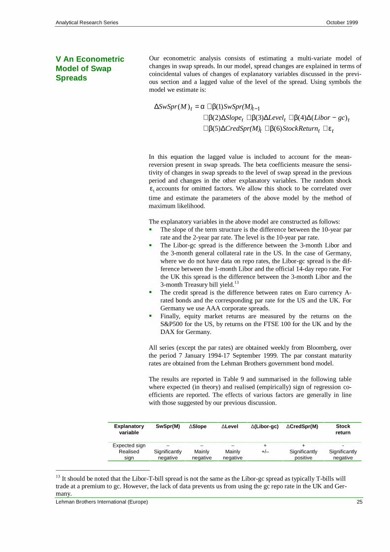
V An EconometricModel of SwapSpreads

Our econometric analysis consists of estimating a multi-variate model ofchanges in swap spreads. In our model, spread changes are explained in terms ofcoincidental values of changes of explanatory variables discussed in the previ-ous section and a lagged value of the level of the spread. Using symbols themodel we estimate is:

ttt

ttt

tt

ReturnStockCredSpr(M)

gcLiborLevelSlope

SwSpr(M)MSwSpr

ε+β+∆β+−∆β+∆β+∆β+

β+α=∆ −

)6()5(

)()4()3()2(

)1()( 1

In this equation the lagged value is included to account for the mean-reversion present in swap spreads. The beta coefficients measure the sensi-tivity of changes in swap spreads to the level of swap spread in the previousperiod and changes in the other explanatory variables. The random shock

tε accounts for omitted factors. We allow this shock to be correlated over

time and estimate the parameters of the above model by the method ofmaximum likelihood.

The explanatory variables in the above model are constructed as follows:� The slope of the term structure is the difference between the 10-year par

rate and the 2-year par rate. The level is the 10-year par rate.� The Libor-gc spread is the difference between the 3-month Libor and

the 3-month general collateral rate in the US. In the case of Germany,where we do not have data on repo rates, the Libor-gc spread is the dif-ference between the 1-month Libor and the official 14-day repo rate. Forthe UK this spread is the difference between the 3-month Libor and the3-month Treasury bill yield.13

� The credit spread is the difference between rates on Euro currency A-rated bonds and the corresponding par rate for the US and the UK. ForGermany we use AAA corporate spreads.

� Finally, equity market returns are measured by the returns on theS&P500 for the US, by returns on the FTSE 100 for the UK and by theDAX for Germany.

All series (except the par rates) are obtained weekly from Bloomberg, overthe period 7 January 1994-17 September 1999. The par constant maturityrates are obtained from the Lehman Brothers government bond model.

The results are reported in Table 9 and summarised in the following tablewhere expected (in theory) and realised (empirically) sign of regression co-efficients are reported. The effects of various factors are generally in linewith those suggested by our previous discussion.

Explanatoryvariable

SwSpr(M) ∆Slope ∆Level ∆(Libor-gc) ∆CredSpr(M) Stockreturn

Expected sign – – – + + -Realised

signSignificantly

negativeMainly

negativeMainly

negative+/– Significantly

positiveSignificantly

negative

13 It should be noted that the Libor-T-bill spread is not the same as the Libor-gc spread as typically T-bills willtrade at a premium to gc. However, the lack of data prevents us from using the gc repo rate in the UK and Ger-many.



Table 9 also shows the estimates of the coefficients for the sample beforeand after July 1998.

The lagged swap spread always has a negative and significant coefficient.These coefficients capture the mean reversion in swap spreads that wedocumented in the section IV. Moreover, as discussed in section III, themean-reversion tends to be lower before July 1998.

There is clear evidence that credit spreads are an economically significantdriver of swap spreads and that their role has increased markedly since thefinancial crisis of 1998. The negative relation of swap spreads and equityreturns is also shown in our estimates, although the high volatility of equityreturns relative to the spread volatility makes the estimates of this relationimprecise.

The slope of the yield curve and the level of yields both have a negative ef-fect, as expected. These effects are pronounced for longer maturities. The ef-fect of the Libor-gc spread is positive and significant for the shortest matur-ity. This is consistent with the idea that the swap spread carry trade — de-scribed in the section IV — is less risky for shorter maturities. One reasonwhy this spread does not show up with more significance may be the error intheir measurements for the UK and Germany where we do not have clean gcrepo rate data.

Since the lagged swap spreads, changes in credit spreads and equity marketreturns are the variables that are most significant in the above regression, weprovide in the appendix — the parameter estimates for a reduced modelwhich only has these variables as explanatory variables.

Overall we conclude that the variables we use explain a large portion of the

variance of swap spreads (2R in the range of 20 to 40%), and, broadlyspeaking, have regression coefficients of the expected sign. The F-test ofjoint significance always rejects the null hypothesis of no explanatory power.14

14 The auto-correlation co-efficient of the errors is estimated to be negative. This indicates that the deviations ofswap spreads from their theoretical values tend to correct themselves gradually over time.



Table 9 Full model regressionsGermanyChange in 2-year swap spreads

Constant SwSpr2(t-1) ∆Slope(t) ∆Level(t) ∆Libor-GC(t) ∆CredSpr2(t) StockRet(t) Estimated rho R2

Full sample 0.839 -0.071 0.002 -0.032 -0.001 0.052 3.555 -0.316 0.191Jan94-Jun98 0.760 -0.070 -0.003 -0.022 -0.019 0.042 -0.318 -0.345 0.203Jul98-Sep99 2.632 -0.170 0.028 -0.063 0.126 0.532 4.259 -0.001 0.371

Change in 5-year swap spreads

Constant SwSpr5(t-1) ∆Slope(t) ∆Level(t) ∆Libor-GC(t) ∆CredSpr5(t) StockRet(t) Estimated rho R2

Full sample 2.793 -0.172 -0.071 0.026 -0.023 0.138 -10.698 -0.309 0.278Jan94-Jun98 2.722 -0.168 -0.073 0.050 -0.035 0.118 -19.210 -0.284 0.285Jul98-Sep99 4.456 -0.253 -0.042 -0.044 0.025 0.563 -1.019 -0.323 0.469

Change in 10-year swap spreadsConstant SwSpr10(t-1) ∆Slope(t) ∆Level(t) ∆Libor-GC(t) ∆CredSpr10(t) StockRet(t) Estimated rho R2

Full sample 1.228 -0.067 -0.064 -0.018 0.004 0.079 -11.199 -0.303 0.186Jan94-Jun98 2.421 -0.164 -0.043 -0.002 0.003 0.040 -4.449 -0.298 0.226Jul98-Sep99 3.938 -0.147 -0.095 -0.055 0.004 0.523 -8.739 -0.379 0.385

United Kingdom


Full sample 0.879 -0.023 0.050 -0.053 0.038 0.154 -21.260 -0.252 0.217Jan94-Jun98 1.996 -1.688 1.299 -1.228 1.962 4.992 0.420 -0.313 0.261Jul98-Sep99 4.879 -0.094 0.039 -0.085 -0.013 0.431 -41.582 -0.137 0.303

Change in 5-year swap spreadsConstant SwSpr5(t-1) ∆Slope(t) ∆Level(t) ∆Libor-GC(t) DCredSpr5(t) StockRet(t) Estimated rho R2

Full sample 0.733 -0.014 -0.098 0.007 0.015 0.297 -57.103 -0.335 0.377Jan94-Jun98 1.260 -0.054 -0.150 0.107 0.007 0.266 14.184 -0.276 0.424Jul98-Sep99 5.395 -0.069 -0.074 -0.142 0.168 0.643 -60.617 -0.349 0.560


Full sample 0.527 -0.006 -0.073 -0.037 -0.020 0.088 -65.631 -0.367 0.236

Jan94-Jun98 1.764 -0.061 -0.104 0.046 -0.003 0.047 -2.355 -0.298 0.195

Jul98-Sep99 3.393 -0.042 -0.072 -0.123 0.000 0.569 -38.388 -0.473 0.598

United States


Full sample 1.240 -0.037 -0.069 0.019 0.024 0.084 -36.149 -0.195 0.107

Jan94-Jun98 1.240 -0.049 -0.126 0.038 0.055 0.126 -23.991 -0.397 0.295

Jul98-Sep99 16.469 -0.376 0.138 -0.087 0.014 0.036 -3.021 0.434 0.192


Full sample 0.987 -0.022 -0.048 -0.048 -0.008 0.080 -33.749 -0.189 0.119

Jan94-Jun98 1.852 -0.061 -0.073 -0.012 0.000 0.046 -30.383 -0.373 0.234

Jul98-Sep99 12.036 -0.213 0.126 -0.199 0.002 0.141 -4.521 0.204 0.376


Full sample 1.578 -0.036 -0.013 -0.042 -0.023 0.096 -43.772 -0.345 0.184

Jan94-Jun98 5.104 -0.158 -0.023 -0.032 -0.032 0.051 -34.927 -0.441 0.311

Jul98-Sep99 6.993 -0.123 0.021 -0.075 -0.009 0.206 -34.316 0.049 0.245

Note: Bold means significant at 5% level; italics means significant at 10% level. Rho denotes the auto-correlation coefficient of theerrors.



V Conclusions We have documented the dynamics of swap spreads across three countries,Germany, the UK and the US. We have also provided an analysis of the eco-nomic drivers of swap spreads. We have shown that the main economic driversof swap spread can be classified into:� credit risk premium related variables (Libor-gc spreads and credit spreads)� yield curve related variables (the level of yields and the slope of the gov-

ernment curve)� variables measuring the level of risk in financial markets.

In addition we have documented a number of institutional factors in themarkets we examined that give rise to demand-supply imbalances impingingon the dynamics of swap spreads. It has been shown that since the financialcrisis of autumn 1998 there may have been a regime shift in the behaviour ofthese spreads. Swap spread levels and volatilities have increased signifi-cantly, as have their correlations across countries and their correlation withcredit spreads. An increase in investor and dealer risk aversion, the reductionin leverage of risk capital employed by relative-value hedge funds (whichwere typical receivers on swaps), a perception of increased risk in asset mar-kets and increases in spread volatility induced by lower liquidity could all becited as factors that have contributed to the recent spread widening.

Euro-area swap spreads continue to remain at half the levels of their UK andUS counterparts. Lower credit spreads in Europe and lower Libor-gc spreads— which in turn could be the result of bank deposits being the dominantavenue for short-term investing in Europe, the somewhat higher credit qual-ity of European banks and a dearth of European credit bonds — may partlyexplain this feature. The issuance of credit bonds in Europe, the risk appetiteof dealers and hedge funds, the shrinking supply of Treasury securities in theUS, the performance of global (especially US) equity markets and cyclicalmovements in the US economy relative to the European economy are alllikely to be the key drivers of swap spreads in the near to intermediate term.

The importance of swaps is now recognised widely as hedging instruments,as instruments for implementing yield curve, credit spread and relative valueviews and as instruments linking treasury, credit and money markets glob-ally. Given this the findings documented here on their empirical behaviourare expected to be useful to investors participating broadly in swap and fixedincome markets.

Appendix This appendix reports the parameter estimates of the following reduced-formversion of our full regression model (section V):

ttt

tt

ReturnStockCredSpr(M)

SwSpr(M)MSwSpr

ε+β+∆β+β+α=∆ −

)3()2(

)1()( 1

Results are given in Table 10. These are consistent with those given in Table9. Additionally, parameters are estimated with greater precision.



Table 10 Reduced model regressions

GermanyChange in 2-year swap spreads

Constant SwSpr2(t-1) ∆CredSpr2(t) StockRet(t) Estimated rho R2

Full Sample 0.757 -0.063 0.065 5.859 -0.328 0.180Jan94-Jun98 0.694 -0.064 0.053 3.141 -0.358 0.195Jul98-Sep99 1.770 -0.116 0.628 5.950 -0.190 0.325Change in 5-year swap spreads


Full Sample 2.812 -0.175 0.124 -9.282 -0.322 0.262Jan94-Jun98 2.630 -0.163 0.092 -20.177 -0.312 0.261Jul98-Sep99 3.925 -0.227 0.642 -0.014 -0.356 0.444Change in 10-year swap spreads


Full Sample 1.366 -0.077 0.099 -7.160 -0.297 0.160Jan94-Jun98 2.560 -0.175 0.045 -0.821 -0.300 0.213Jul98-Sep99 4.198 -0.163 0.550 -6.971 -0.334 0.331

United KingdomChange in 2-year swap spreads


Full Sample 0.772 -0.020 0.179 -12.833 -0.245 0.194Jan94-Jun98 0.729 -0.025 0.148 10.846 -0.310 0.242Jul98-Sep99 5.211 -0.099 0.444 -45.934 -0.132 0.273Change in 5-year swap spreads


Full Sample 0.832 -0.016 0.324 -53.819 -0.357 0.359Jan94-Jun98 1.302 -0.047 0.277 -18.211 -0.344 0.367Jul98-Sep99 5.060 -0.066 0.699 -58.625 -0.344 0.480Change in 10-year swap spreads


Full Sample 0.640 -0.008 0.130 -52.202 -0.380 0.195Jan94-Jun98 1.595 -0.050 0.058 -14.406 -0.291 0.120Jul98-Sep99 3.559 -0.046 0.681 -30.553 -0.464 0.531

United StatesChange in 2-year swap spreads


Full Sample 1.269 -0.036 0.069 -38.196 -0.203 0.093Jan94-Jun98 1.214 -0.042 0.091 -38.847 -0.380 0.219Jul98-Sep99 14.219 -0.323 0.045 0.417 0.146 0.328Change in 5-year swap spreads


Full Sample 1.093 -0.026 0.089 -21.958 -0.195 0.076Jan94-Jun98 1.749 -0.056 0.048 -25.893 -0.352 0.197Jul98-Sep99 12.473 -0.222 0.204 6.617 0.055 0.194Change in 10-year swap spreads


Full Sample 1.573 -0.037 0.104 -34.002 -0.327 0.164Jan94-Jun98 4.861 -0.151 0.057 -21.975 -0.430 0.296Jul98-Sep99 7.376 -0.132 0.192 -24.232 0.138 0.198

Note: Bold means significant at 5% level; italics means significant at 10% level. Rho denotes the auto-correlationcoefficient of the errors.

Lehman Brothers International (Europe) is regulated by the Securities and Futures Authority. This document is for information purposes only and should not be regarded as an offer tosell or a solicitation of any offer to buy the products mentioned herein. The information in this document has been obtained from sources believed to be reliable, but we do not representthat it is accurate or complete and it should not be relied upon as such. Lehman Brothers International (Europe), its affiliated companies, shareholders, directors, officers, and/or employeesmay have long or short positions in the securities or commodities mentioned in this document, or in options, futures and other derivative instruments based thereon. It is possible thatthe individuals employed by Lehman Brothers International (Europe), or its affiliates may disagree with the recommendations or opinions in this document. Lehman Brothers International(Europe), or its affiliates may, from time to time, effect or have effected an own account transaction in, or make a market or deal as principal in or for, the securities or commodities mentionedin this document, or in options, futures or other derivative instruments based thereon. Lehman Brothers International (Europe), or its affiliates may have managed or co-managed a publicoffering of the securities mentioned in this document within the last three years, or may, from time to time, perform investment banking or other services for, or solicit investment bankingor other business from, any company mentioned in this document. ©1999 Lehman Brothers International (Europe), Lehman Brothers Inc.

Analytical Research Series - INSEADfaculty.insead.edu/joel-peress/documents/dynamics... ·...

Documents

Transcript of Analytical Research Series - INSEADfaculty.insead.edu/joel-peress/documents/dynamics... ·...