27TH

INTERNATIONAL CONGRESS OF THE AERONAUTICAL SCIENCES

1

Abstract

In this paper, a procedure to develop an analytical two-term truncated Volterra series for the low order flight subsystems is presented. The resultant models are given in the form of first and second kernels. A parametric study of the influence of each linear and nonlinear term on kernel structures is investigated. A step input is then employed to quantify and qualify the nonlinear response characteristics. Uniaxial surge and pitch motions are presented as examples of the low order flight dynamic systems. The proposed analytical Volterra-based model offers an efficient nonlinear preliminary design tool in qualifying the aircraft responses before computer simulation is invoked or available.

1 Introduction

Constructing an analytical model describing nonlinear aircraft dynamic behavior has been investigated using various approximation techniques. Three common approaches appear in the literature to predict nonlinear phenomena: bifurcation approach, describing function approach, and perturbation expansion approach. Bifurcation analysis has been applied to many nonlinear phenomena such as wing rock [1-5], spin entry [6-7], and pilot-induced oscillation [8]. Describing function analysis has been used mostly to generate limit cycle behavior in many flight dynamic models as reported in Refs. [8-12]. Since perturbation expansion analysis breaks down quickly in time or in parameter strength. One example is given in Ref. [13]. Although all these techniques show potential to understand and analyze nonlinear behavior of aircraft, these methods sometimes do not provide a precise cause-and-effect result, do not address transient behavior, or do not cover a sufficient range of time and/or parameter variation.

Volterra theory has emerged as a popular nonlinear modeling technique, primarily because of the underlying analytical framework and its extension of the impulse response concept from linear theory. Volterra theory dates back to 1887 with the first encompassing publication appearing in 1927 and later in 1958 [14-15]. An early use of this theory was made by Wiener and subsequent research was conducted at the Massachusetts Institute of Technology in the area of filtering and electronic circuits [16-18]. Few applications of the Volterra methodology to flight mechanics appear in the literature. References [19-20] are two notable exceptions. In these efforts, modeling the longitudinal dynamics of a high performance aircraft in limit cycling conditions has been explored via the Volterra approach. In Ref. [20], a differential form of a reduced third order Volterra series was considered. The approach proved the ability to capture the limit cycle. This work was extended in Ref. [19] to a global approach. An interesting application of Volterra theory in flight mechanics is presented in Ref. [21] to analytically define nonlinear flying quality metrics. However, most of these trials date back to the 1980s and early 1990s. Recently, in Refs. [22-23], the authors bring back the utilization of Volterra theory to flight mechanics through a global piecewise approach. This approach facilitates the use of Volterra theory in a piecewise fashion for strong nonlinearity. Continuing this effort of utilizing Volterra theory in flight mechanics research, a new trial to use the theory in analytically predicting nonlinear behavior is investigated herein.

This paper presents an analytical framework to predict the nonlinear behavior of the first and second order SDOF flight subsystems. Section 2 shows that the essence of aircraft nonlinear behavior in multi-axis motion can be rendered with simple first order and second order single degree of freedom (SDOF) submodels. In Sections 4, the outline of developing a closed

ANALYTICAL NONLINEAR ANALYSIS METHODOLOGY FOR REDUCED AIRCRAFT DYNAMICAL SYSTEMS

Ashraf Omran and Brett Newman

Department of Aerospace Engineering, Old Dominion University, Norfolk, VA 23529

Keywords: Volterra theory, Uniaxial Motion, Nonlinear Dynamics.

Ashraf Omran and Brett Newman

2

form solution based on Volterra theory is briefly discussed. Sections 4-5 provide generalized closed form solutions to the first and second order SDOF systems previously developed in Section 2. More specifically, the nonlinear step response of the low order systems is investigated in Section 6-7 to qualify and quantify these low order subsystems behavior. In Section 8, numerical examples are presented to assess the proposed Volterra-based models. The work is finally concluded in Section 9.

2 Low order uniaxial flight subsystems

This section shows how the full order aircraft dynamic model can be represented as a set of low order flight dynamic subsystems while preserving the link to the more general model. The two low order system examples: surge and pitch motions, are offered herein as demonstrations. Each example represents a SDOF uniaxial motion. Reference [24] contains a frequently cited full order dynamic model of a high performance aircraft. This model is considered under many assumptions: the aircraft is a rigid body with six degrees of freedom (6DOF) except for an internal constant spinning engine rotor, the aircraft mass is constant, the aircraft body is symmetric about the XZ plane, the atmosphere is stationary, and the earth is flat with constant gravity. Based on those assumptions the nonlinear equations of motion, derived from Newtonian mechanics, are

m

TC

m

Sqgqwrvu

TX sin (1)

TYCm

Sqgrupwv sincos (2)

TZCm

Sqgpvquw coscos

(3)

TL

XX

XZ

X

ZY CI

Sbqpqr

I

Iqr

I

IIp

(4)

rHCI

cSqpr

I

Ipr

I

IIq eM

YY

XZ

Y

XZ

T

22 (5)

qHCI

Sbqqrp

I

Ipq

I

IIr eN

ZZ

XZ

Z

YX

T

(6)

The aerodynamic and engine data used in the aircraft model have been developed by a test at NASA Langley Research Center in 1979 as listed in Ref. [24]. This test was conducted in low-speed wind tunnel facilities. The model data represents the total aerodynamic coefficients (

TTTTTT NMLZYX CCCCCC ,,,,, ) as function of angle of attack α, sideslip angle β, elevator deflection δe, aileron deflection δa, and

rudder deflection δr as look-up tables. However, the model is computationally expensive. In Ref. [25], a simplified model of the aerodynamic coefficients is represented. The new model has the capability to reduce the computational cost with an acceptable accuracy, but the simplicity of this model restricts the angle of attack range to -10

o /+45

o and the sideslip angle range to -

30o/+30

o. The equivalent aerodynamic tables of

this model are given in Ref. [25]. All tabular data are valid only for the limits on the angle of attack, sideslip angle, and control surfaces (|δe| < 25, | δa| < 25, and | δr | < 25). The maximum thrust (T) of the afterburner turbofan engine model is given as a function of altitude H, Mach number M, and throttle deflection δth. The numerical values of the engine model are given in Refs. [24-25].

The dominant behavior of a conventional aircraft can be fairly well described by a symmetric motion (longitudinal) and an asymmetric motion (lateral-directional), if the engine angular momentum He is assumed zero. In the case of symmetric longitudinal flight, the lateral-directional variables are exactly zero due to airplane symmetry about the XZ plane. Using the stability axes and the relations w = V sin(α), u = V cos(α), and V

2 = u

2 + w

2, one can replace

the surge u and heave w equations by the total velocity V and the angle of attack α equations. A reduced nonlinear longitudinal model can then describe the aircraft motion as

sin,,,

cosgC

m

SqHMT

mV eDth (7)

cos,,,

sin

V

gC

mV

SqHMT

mVq eLth

(8)

eM

YT

CI

cSqq ,0, (9)

q (10)

where

sincos

sincos

TT

TT

XZL

ZXD

CCC

CCC

(11)

If an autopilot is assumed to hold the altitude to a constant value Ho and the flight path angle γo = θo - αo at zero value, then the total velocity variation is given as

ˆ,,

,2

,,cos 2

th

eooDtho

o

Vf

Cm

SVHVT

mV

(12)

where αo and eo are the trimmed angle of

attack and elevator deflection, which are determined by the specified parameter vector ̂ = [Ho Vo]

T. Equation (12) represents a first

order SDOF system for total velocity with the throttle deflection as the input. The perturbation

3

ANALYTICAL NONLINEAR ANALYSIS ETHODOLOGY FOR REDUCED AIRCRAFT DYNAMICAL SYSTEMS

form of Eq. (12) is given by introducing the derivatives of the function f as

ˆ !2

1ˆ

ˆ!2

1ˆˆ

2

2

22

2

2

2

th

th

th

th

th

th

fV

V

f

VV

ffV

V

fV

(13)

The two perturbed quantities ΔV and Δδth, not necessarily small, are measured from the nominal values defined at the operating condition. Since the aerodynamic and engine models of the aircraft are given in the form of look-up tables, a finite difference technique is the proper choice to compute the derivatives appearing in Eq. (13). Another example of a longitudinal low order flight subsystem is the nonlinear pitching motion. In this pitching motion, the total velocity is assumed constant in magnitude (V = Vo) and direction (γ = γo = 0, θ = α). The pitch motion is then described by a second order SDOF subsystem as

ˆ,,,,, eeM

Y

qfqCI

cSqq

q

T

(14)

The parameter vector ̂ is introduced through q . Expanding the nonlinear function f around the nominal point, defined by ̂ , leads to

2

2

22

222

2

2

2

2

2

ˆ!2

1 ˆ

ˆˆ ˆ!2

1

ˆ!2

1ˆˆˆ

e

e

e

e

e

e

e

e

fq

q

f

fq

q

fq

q

f

ffq

q

ffq

q

(15)

The perturbed quantities Δθ, Δq and Δδe are defined from the nominal value determined by the operating condition ̂ = [Ho Vo]

T.

The two uniaxial flight examples of surge and pitch motions represent the aircraft behavior as a SDOF first or second order system. In Ref. [29], the authors developed another two equivalent examples for the lateral motion. The nonlinearity herein appears in the high order aerodynamic and propulsive derivatives with respect to the input and state signals. The linear theory offers an analytical solution for such low order systems, which counts the first order derivatives only. When the aircraft operates at unusual attitudes, the first order derivatives are insufficient to render the behavior. Volterra theory is used herein as a nonlinear approximate technique to develop an analytical solution in order to count these high order derivatives for the first and second order SDOF systems as shown in the next Sections.

3 Volterra theory

Many physical systems can be described across a set of nonlinear differential and algebraic equations between the input signal

mRu , the state signal nRx , and the output

signal pRy . A commonly used representation is the nonlinear state space form

tutxtgty

tutxtftx

,,

,,)(

(16)

Vectors nRf and pRg denote the system

nonlinearities and 1Rt is time. Volterra theory represents the input-output relation of a nonlinear system as an infinite sum of multi-dimensional convolution integrals [15].

ii

k

k

i

kko dtuhthty

1 0 0 0 1

21 ,...,,.... (17)

In Eq. (17), kkh ,...,, 21 denotes the kth

order Volterra kernel. Volterra kernels are casual functions with respect to their argument [15]. For developing analytical Volterra kernels from the nonlinear differential equation, the variational expansion form, also called the differential form, is used. Variational method was initially developed based on a perturbation point of view with the first notable application in Ref. [27] and it showed the capability to capture the aircraft behavior in many nonlinear phenomena in Refs. [19-23]

Before applying the differential method to the low order flight systems in Section 2, the outline of the method for a single input case is first given to show the mechanism by which the analytical kernels can be constructed. The method assumes the state vector derivative x is expandable as an infinite power series in terms of the state vector

nRx and scalar input 1Ru around an arbitrary point, defined by

(xo,uo), as

0 0

~,

i j

ji

ij uxKuxfx ,

1

1

i

k

i xxx (18)

In Eq. (18), is the Kronecker product. The Kronecker product for two matrices P of dimension NPMP and Q of dimension NQMQ is defined as [15]

QPQP

QPQP

QP

PpP

P

MNN

M

1

111

(19)

The resultant matrix QP is of the size (NP

NQ) (MPMQ). The matrix ijK

~ of size nni is

defined as

Ashraf Omran and Brett Newman

4

,,,, i,j

KK

KK

K

ijnnijn

ijnij

ij

i

i

210 ,~

1

111 (20)

Note00

~K has a null value. Thus, the expansion

holds around an equilibrium point ( x = 0). The matrix

ijK~ represents the derivatives of the

vector function f(x,u) with respect to x(i)

and uj

at point (xo,uo). The input u is generalized to be αu(t), where α is any arbitrary constant. In this case, the response x(t) can be expanded in terms of α as

1i

i

i xx (21)

By substituting in Eq. (18) and rearranging according to the coefficients of equal α

i (i = 1, 2,

…), a set of differential equations is generated as

122120

)3(

1303103

2

02111

)2(

1202102

011101

~~~

~~~~

~~

xxxxKxKxKx

uKuxKxKxKx

uKxKx

(22)

Equation (22) represents the system as an infinite set of differential equations. Although this expansion extends the n-dimensional problem to infinite dimension, the original nonlinearity of the system is broken down into a sequence of pseudo-linear time invariant (PLTI) systems, which are solvable. The input of each PLTI system is a nonlinear function of all previous system states and the input u. Figure 1 shows the schematic diagram of the method for the PLTI systems through the k

th term. The first

PLTI system has a linear transition matrix Φ(t-t0) based on the square matrix 10

~K , which is

excited by input u multiplied the column vector

01K~ . The state response of this system, x1, in

closed-form is a convolution integration in terms of u and t, which is mapped to the next system by a nonlinear function f1(x1,u). This sequence is repeated for a certain number k, which provides satisfactory results. Note that fi-1

(x1,x2,…,xi-1,u), where i = 1,2,…,k, automatically keeps the order of input u to the power i. For example, f1(x1,u) is a sum of u

2,

x1u, and )2(

1x . By substituting for x1 as a convolution integral of u, the bilinear term, x1u, and the state quadratic term, )2(

1x , become a function of u

2. Then, x2 is defined as a

convolution integral of u2. In general, this

condition is not essential to the method, but it is necessary to extract the kernels. Thus, each state response of the PLTI systems, xi, conceptually yields the kernel hi(τ1,.., τi) as described in the next two Sections.

Figure 1 Variational expansion method schematic diagram

3 First order system generalized solution

The surge motion in Eq. (13) and another roll motion presented in Ref. [29] are examples of the SDOF first order flight system. The generalized equation of motion of such systems is

3

03

2

12

2

02

2

21

1101

3

30

2

2010

0 0

ukxukukuxk

xukukxkxkxkuxkx ji

i j

ij (23)

where kij is the corresponding coefficient to the term x

iu

j and i, j = 0,1,2,3,…. and k00 = 0. Based

on the global Volterra approach in Refs. [22-23], a small set of linear and nonlinear terms is enough to specify the system characteristics in a certain domain. Therefore, the quadratic state, bilinear state-input, and quadratic input terms in addition to the linear terms in Eq. (23) are considered to be sufficient. As a function of these terms, the system is

2

0211

2

2001 ukxukxkukaxx (24)

Note the linear state term coefficient has been re-symbolized by a instead of k10. This re-symbolization has the purpose to emphasize the uniqueness of this term more than others, as clearly indicated later in this Section.

The variational method is now applied to develop the Volterra kernels. The state x can be then expressed as a

3

3

2

2

1 xxxx (25)

By substituting in Eq. (24) and equating αi

coefficients, where i = 1,2,3, … , a set of pseudo differential equations is generated as

2

112

2

121211212033

2

02111

2

12022

0111

2 uxkuxkuxkxxkaxx

ukuxkxkaxx

ukaxx

(26)

The solution of the first differential equation of

x1 with a zero initial condition is

duekx

t

ta

0

011 (27)

5

ANALYTICAL NONLINEAR ANALYSIS ETHODOLOGY FOR REDUCED AIRCRAFT DYNAMICAL SYSTEMS

The solution of x2 is then given as

qibsiqs

t

ta

t

ta

t

ta

xxx

duek

duxekdxekx

222

2

0

02

0

111

0

2

1202

(28)

where qibsiqs xxx 222 ,, represent the quadratic state, bilinear state-input, and quadratic input components of x2. Using the convolution solution of x1 from Eq. (27) and substituting in Eq. (28), the quadratic state component qsx2

and the bilinear state-input component bsix2

, are then given as

2121

0

,max

0

2

01202

2121 1 dduueee

a

kkx

t

ttata

t

ta

qs

(29)

t t

ttabsi dduuekk

x0 0

2121

,max0111

221

2

(30)

where max(x,y) refers to the maximum values between x and y. Note the authors documented the required mathematical manipulations to derive Eqs. (29-30) in Refs. [29-31]. The quadratic input component qix2

yields to the standard Volterra form as

2121

0 0

2102

2

0

022

1

dduuek

duekx

t t

ta

t

taqi

(31)

where δ(τ1-τ2) is the impulse function. Adding the quadratic and bilinear

components to the linear term offers an approximate solution of x as

2102

,max0111

,max2

0120

222212011

0 0

2121212

0

1

121

2121

2

1

,,

where

,

aa

aaa

qibsiqsa

t t

t

ekekk

eeea

kk

hhhhekh

dduutth

duthx

(32)

The resultant approximate solution is given by the two kernels h1 and h2. For any arbitrary input u(t), one can compute the response x using convolution integrals or the pseudo state space

representation. These kernels are a unique signature of the first order SDOF system. To understand how the system behavior varies with these parameters, their influence on each kernel is presented next.

The first kernel h1 is an exponential function with a gain k01 and a power factor a. It is clear that this power factor a controls the divergence or convergence of the first kernel histories. In the case of a > 0, the value of h1 keeps increasing with time to be infinite as time tends to infinity. This observation concludes that the system has a divergent or unstable response for any input. If a is null, the first kernel is constant with time, which means that the system linear response is the input integration. In the case of a < 0, at time zero, the value of h1 is k01. This value keeps decreasing with time, yielding zero at time equal to infinity. Figure 2 shows the normalized generic shape of h1 in the case of a < 0. The normalized kernel starts at 1 heading downward with an angle υ = arctan(a). This slope is an indication of the initial or maximum speed by which the system responds to any arbitrary input. If a 2% value is considered as a tolerance for approximate steady state, the required time to be inside this zero vicinity is labeled here as the linear kernel settling time

lks

. This time is computed as a function of a to be

0 < afor

402.0ln

aa

l

ks

(33)

The second kernel has three components: quadratic state kernel

qsh2 , bilinear state-input kernel

bsih2 , and quadratic input kernelqih2 . Each

component is a two dimensional surface as a function of τ1 and τ2. The quadratic state kernel

qsh2 has three exponential terms. The linear coefficient a controls the divergence and convergence of this surface. In the case of a= 0, the surface is defined by

2

0120kk max(τ1, τ2) using l’Hopital’s rule. This maximum operator represents two ramp surfaces τ1 and τ2 merged at the diagonal line, which implies that if the system is critically stable in the linear sense (a = 0), the state quadratic term has a divergent kernel shape (instability). Such a conclusion is not accessible using the linear analysis. When a > 0, the surface starts at the zero value heading upwards to a divergence referring to unstable behavior for any external excitation. If the value of a is negative, the surface starts at zero and diminishes at infinite time arguments τ1 and τ2. The exponential term with the maximum operation in the exponent works on directing the surface upward and enforcing the surface edges to be zero, while the two regular exponential

Ashraf Omran and Brett Newman

6

terms of τ1 and τ2 work on heading the surface downward. The irregular exponential term competes with the two regular terms reaching a maximum surface value at τ1 = τ2 = ln(2)/|a|≈ 0.7/|a|, beyond which this effect diminishes. The two standard exponential terms then dominate the shape of the surface, yielding zero as the two arguments τ1 and τ2 go to infinity. One example of this surface is given in Figure 3, where a = -5 1/s. The overall shape of this kernel is determined by its diagonal (τ1 = τ2). The normalized general shape of this diagonal is shown in Figure 4. The surface has a maximum value 0.25 akk /2

0120 at timeqs

km = ln(2)/|a| ≈ 0.7/|a|. The required time by which the surface is considered as zero is referred to here as the quadratic state kernel’s settling time aqs

ks /4 The surface of the bilinear state-input kernel

component bsih2 is an exponential function,

which includes a maximum operator in the power. The surface heads to zero (stable or convergent) as τ1 and τ2 tend to infinity in the case of a < 0, or head to infinity (unstable or divergent) in the case of a > 0. When a = 0, the normalized surface is a flat one with a value 0.5. Figure 5 shows an example of the bilinear state-input kernel at a = -5 1/s. The diagonal shape of this kernel is the same as the linear first kernel in Figure 2 with a different gain of k01k11/2, but with the same initial slope angle υ = arctan(a) and the same settling time al

ks

bsi

ks /4 . The surface of the quadratic input kernel component

qih2 is an exponential impulse sheet oriented vertically on the diagonal line τ1 = τ2, which has the same shape and characteristics of the first kernel in Figure 2, but with a gain of k02 instead of k01.

Figure 2 First order system first kernel in the case of a < 0

Figure 3 First order system quadratic state second kernel at a = -5

1/s

Figure 4 first order system quadratic state second diagonal kernel in

the case of a < 0

Figure 5 First order system bilinear state-input second kernel at a =

-5 1/s

4 Second order system generalized solution

The pitch motion in Eq. (15) in addition to another yaw motion documented in Ref. [29] are examples of the SDOF second order flight systems. The generalized equations of motion of such systems are

2

002011101001

2

020110

2

200

2

2

ukvukxukuk

vkxvkxkvxv

vx

nn

(34)

7

ANALYTICAL NONLINEAR ANALYSIS ETHODOLOGY FOR REDUCED AIRCRAFT DYNAMICAL SYSTEMS

Parameter klmn is the corresponding coefficient to the term nml uvx and l, m, n = 0,1,2. Note that the linear terms have been re-symbolized by - 2δωn instead of k010 and

2n instead of k100.. This

re-symbolization is for the purpose of keeping the discussion in the sense of undamped natural frequency ωn and damping ratio δ from the linear theory. The variational method is now applied to Eq. (34) to develop the kernels. The method assumes that the input is αu where α is any arbitrary constant. The state position x and state rate v can then be expressed as a sum of infinite terms.

3

3

2

2

1

3

3

2

2

1

vvvv

xxxx

(35)

By equating αi coefficient, a set of pseudo

differential equations is generated:

3

3

2

3

3

2

0021011

1101

2

102011110

2

12002

2

2

2

2

0011

1

2

1

1

2

10

00

00

0

0

2

10

0

2

10

v

x

v

x

ukuvk

uxkvkvxk

xkv

x

v

x

ukv

x

v

x

nn

nn

nn

(36)

The solution of the first linear pseudo subsystem [x1 v1]

T for a zero initial condition is then

computed as

cos

sin1

sin

1

02

0011

0

0011

dutek

v

dutek

x

t

d

t

t

d

t

d

(37)

where n denotes the system’s damping factor and 21 nd

is the damped natural frequency.

For the second pseudo subsystem [x2 v2]T,

the solution of x2 is sought as a sum of six components

qibribsiqrbsrqs xxxxxxx 2222222 (38)

where ,,,,, 22222

bribsiqrbsrqs xxxxx and qix2 are quadratic state, bilinear state-rate, quadratic rate, bilinear state-input, bilinear rate-input, and

quadratic input component respectively. The second pseudo state space is then rewritten as

2

002

1

011

1

101

2

1

020

11

110

2

1

2002

2

2

2

2

0

0

0

0

0

0

2

10

uk

uvk

uxk

vk

vxk

xkv

x

v

x

qibri

bsiqrbsr

qs

BB

BBB

BA

nn

(39)

Substituting the convolution solutions of x1 and v1 from Eq. (37) into Eq. (39), the convolution solutions of the six components of x2 are derived as [29-31]:

213

212211

4

2

001200

212

212121

0 0

22

sin

coscos

2,

,

21

d

dd

d

qs

t t

qsqs

M

MM

eekk

h

dduutthx

(40)

213

212211

32

2

001110212

212121

0 0

22

sin

coscos

12,

,

21

d

dd

d

bsr

t t

bsrbsr

M

MM

eekk

h

dduutthx

(41)

2sin

2coscos

12,

,

213

212211

22

2

001020

212

212121

0 0

22

21

d

dd

d

qr

t t

qrqr

M

MM

eekk

h

dduutthx

(42)

212121

,max

2

101001

212

212121

0 0

22

,min,maxsin,minsin

2,

,

21

ddd

d

bsi

t t

bsibsi

ekk

h

dduutthx

(43)

212121

,max

2

001011

212

212121

0 0

22

,min,maxsin,minsin

12,

,

21

ddd

d

bri

t t

bribri

ekk

h

dduutthx

(44)

Ashraf Omran and Brett Newman

8

211002

212

212121

0 0

22

sin,

,

1

d

d

qi

t t

qiqi

ekh

dduutthx

(45)

where

ˆ,min3cos89

1892

1

,mincos12

1,

ˆ,min3sin99

891

892

13

,minsin1

12

1,

,minsin1

11,

21

,min2

2

2

21

,min2

213

21

,min

2

2

2

2

212

,min2

212

212

,min2

211

21

21

21

21

21

d

d

d

d

d

e

eM

e

eM

eM

and 289/ˆcos . The authors provided a full derivation to the expressions of Eqs. (40-45) in Ref. [29-3129].

The overall second kernel is a sum of the six components quadratic state qsh2

, bilinear state-rate bsrh2

, quadratic rate qrh2, bilinear state-input

bsih2, bilinear rate-input brih2

, and quadratic input qih2

. The resultant second kernel along with the first kernel represents an approximate Volterra-based model for the second order SDOF system.

qibribsiqrbsrqs

t t

t

hhhhhhh

dduutth

duthx

2222222

0 0

2121212

0

1

,

(46)

The Volterra-based model presents the system as two analytical kernels. The analytical expressions of these kernels are used to understand each kernel characteristic as a function of system parameters for the second order SDOF system.

The first kernel h1 is an exponential sinusoidal function with a gain k001/ωd , frequency ωd , and a damping factor σ. If the damping factor is less than zero, then the system lacks the damping required to stabilize the response for any excitation. Thus, the positive exponential power shapes a divergent kernel. When taking the damping factor off (null damping factor), the remaining sine term keeps the kernel shape as an oscillatory one. In the

case of positive damping factor σ > 0, it is better to parameterize the kernel by the damping ratio δ = σ/ωn . If the damping ratio is more than or equal to unity, then the sine term diminishes and the resultant first kernel is a sum of two exponential terms, which is the case in the first order system. These two exponential terms become equal at δ = 1. For less than unity damping ratio 0 < δ < 1, the generic shape of the first kernel is shown in Figure 6. In this case (0 < δ < 1), the kernel starts at zero and oscillates around zero. The amplitude of such oscillation decreases with time, where the loci of minimum and maximum points are located along the envelope functions h1max and h1min.

, 001min1

001max1

t

d

t

d

ek

thek

th

(47)

The maximum points occur at times (2nπ+υ)/ωd, while the minimum points occur at times ((2n+1)π+υ)/ωd, where n = 0,1,2,… The kernel h1 settles down inside a 2% band around zero at time

402.0ln

l

ks (48)

Figure 6 Second order system first kernel in the case of 0 < ζ < 1

The second kernel has six components: qibribsiqrbsrqs hhhhhh 222222 and ,,,,, . Each component

is a two dimensional surface in τ1 and τ2. In the case of negative damping factor σ, all the surfaces have zero edges heading upwards to infinity as τ1 and τ2 go to infinity. These divergent surfaces have a sinusoidal waveform with a frequency ωd in the case of -1 < δ < 0 (oscillatory divergent). This sinusoidal waveform diminishes when δ -1 (non-oscillatory divergent). All surfaces become a constant amplitude two-dimensional sinusoidal surface in the case of zero damping ratio δ = 0 (oscillatory). No parametric studies are given to the unstable or critically stable cases, since these cases have a divergent response, which

9

ANALYTICAL NONLINEAR ANALYSIS ETHODOLOGY FOR REDUCED AIRCRAFT DYNAMICAL SYSTEMS

does not require to be characterized. Thus, the characterization is sought for a stable behavior for the design and control purposes. If the damping ratio is more than unity δ 1 (non-oscillatory convergent), all the surfaces turn to a sum of two exponential functions and the analysis of the first order system in Section IV can then be used. In the case of 0 < δ < 1 (oscillatory convergent), which is the frequent case of the aircraft low order motions, all the surfaces have a two-dimensional damped sinusoidal waveform. One example is given in Figures 7-11 at δ = 0.1 and ωn = 2 rad/s. The quadratic input component , as a special case, is an impulsive surface over the diagonal line τ1= τ2 having the same shape as the first kernel but with a gain of k002/ωd.

Figure 7 Second order system quadratic state kernel at ζ = 0.1and

ωn = 2 rad/s

Figure 8 Second order system bilinear state-rate kernel at ζ = 0.1

and ωn = 2 rad/s

Figure 9 Second order system quadratic rate kernel at ζ = 0.1 and

ωn = 2 rad/s

Figure 10 Second order system bilinear state-input kernel at ζ = 0.1

and ωn = 2 rad/s

Figure 11 Second order system bilinear rate-input kernel at ζ = 0.1

and ωn = 2 rad/s

In order to characterize each surface in the case of 0 < δ < 1, the diagonal waveform

,2

jh , where j = {qs, bsr, qr, bri}, is considered, while the diagonal waveform of

5.0,2

bsih is considered. Thus, the diagonal line of ,2

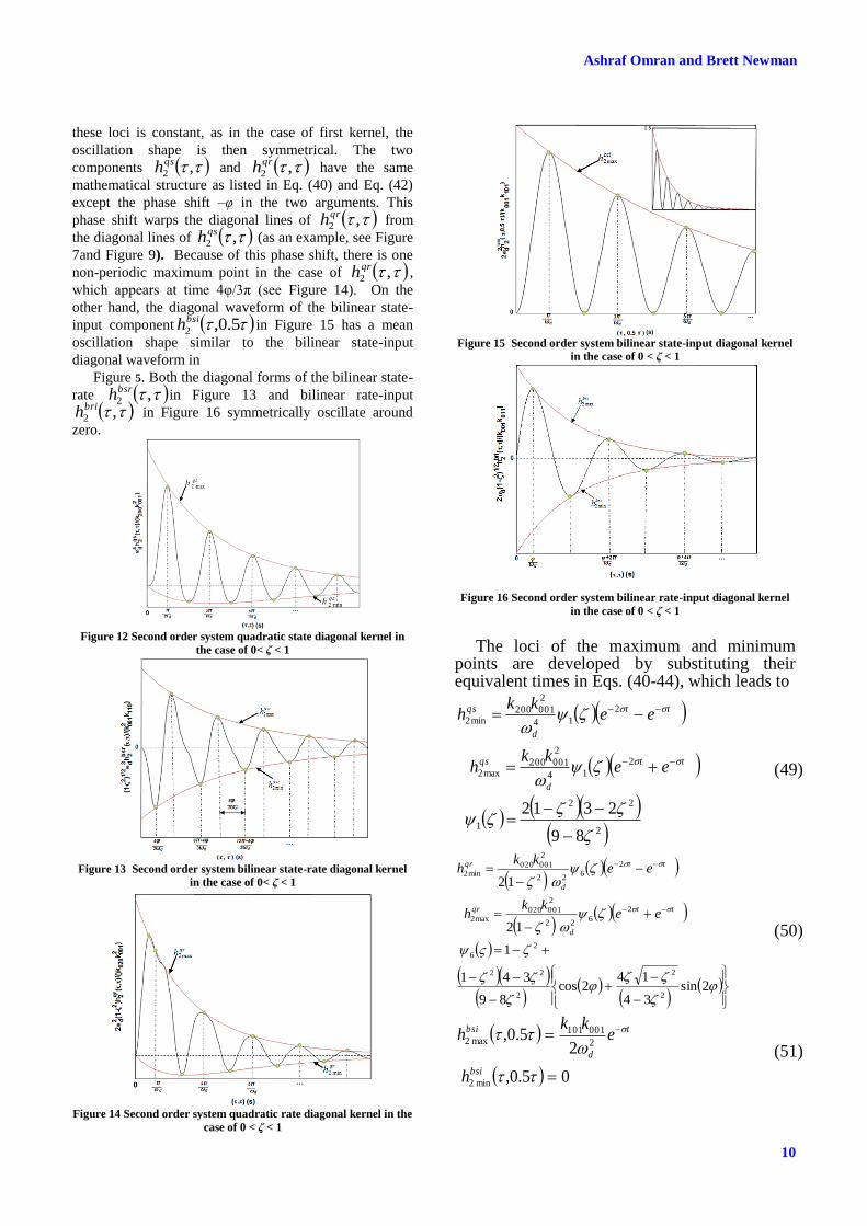
bsih has a zero waveform. Figures 12-16 show the generic shapes of these diagonal waveforms. All the diagonal histories start at zero value and oscillate by a frequency ωd generating a set of minimum and maximum value at times listed in Table 1.

Table 1 The times of maximum and minimum values of the second

kernel’s components, where n = 0, 1, 2, …

Although all the diagonal waveforms settle at zero by

time t = , the equivalent oscillation shapes to reach

this zero value are not the same. Both quadratic state

,2

qsh in Figure 12 and quadratic rate ,2

qrh in

Figure 14 do not symmetrically oscillate around the zero

value. The mean oscillation shapes of ,2

qsh and

,2

qrh are similar to the one in Figure 4 (the quadratic

state diagonal kernel of the first order system). The mean

oscillation shape is sought here as the average of the

maximum and minimum points’ loci. If the average of

Ashraf Omran and Brett Newman

10

these loci is constant, as in the case of first kernel, the

oscillation shape is then symmetrical. The two

components ,2

qsh and ,2

qrh have the same

mathematical structure as listed in Eq. (40) and Eq. (42)

except the phase shift –υ in the two arguments. This

phase shift warps the diagonal lines of ,2

qrh from

the diagonal lines of ,2

qsh (as an example, see Figure

7and Figure 9). Because of this phase shift, there is one

non-periodic maximum point in the case of ,2

qrh ,

which appears at time 4φ/3π (see Figure 14). On the

other hand, the diagonal waveform of the bilinear state-

input component 5.0,2

bsih in Figure 15 has a mean

oscillation shape similar to the bilinear state-input

diagonal waveform in

Figure 5. Both the diagonal forms of the bilinear state-

rate ,2

bsrh in Figure 13 and bilinear rate-input

,2

brih in Figure 16 symmetrically oscillate around

zero.

Figure 12 Second order system quadratic state diagonal kernel in

the case of 0< ζ < 1

Figure 13 Second order system bilinear state-rate diagonal kernel

in the case of 0< ζ < 1

Figure 14 Second order system quadratic rate diagonal kernel in the

case of 0 < ζ < 1

Figure 15 Second order system bilinear state-input diagonal kernel

in the case of 0 < ζ < 1

Figure 16 Second order system bilinear rate-input diagonal kernel

in the case of 0 < ζ < 1

The loci of the maximum and minimum

points are developed by substituting their equivalent times in Eqs. (40-44), which leads to

89

2312

2

22

1

2

14

2

001200max2

2

14

2

001200min2

tt

d

qs

tt

d

qs

eekk

h

eekk

h

(49)

2sin34

142cos

89

341

1

12

12

2

2

2

22

2

6

2

622

2

001020max2

2

622

2

001020min2

tt

d

qr

tt

d

qr

eekk

h

eekk

h

(50)

05.0,

2

5.0,

min2

2

001101max2

bsi

t

d

bsi

h

ekk

h

(51)

11

ANALYTICAL NONLINEAR ANALYSIS ETHODOLOGY FOR REDUCED AIRCRAFT DYNAMICAL SYSTEMS

ˆ3/sin89

1

3/7sin23/4sin2

1

3/11sin14

3/11cos438989

1

3

4sin

89

1

2

1

ˆ3

7sin

2

1

3sin1

3

5sin

89

14

3

5cos

89

4311

12

12

2

2

5

2

22

2

2

4

2

2

2

3

2

2/32

2

222

2

5

2

432

2

001110min2

3

2

232

2

001110max2

tt

d

bsr

tt

d

bsr

eekk

h

eekk

h

(52)

t

d

bri

t

d

bri

ekk

h

ekk

h

2

001011min2

2

001011max2

12,

12,

(53)

where jh min2 and jh max2

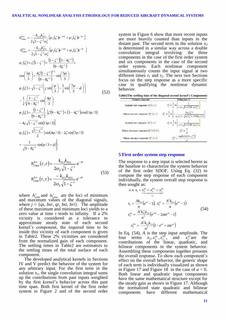
are the loci of minimum and maximum values of the diagonal signals, where j = {qs, bsr, qr, bsi, bri}. The amplitude of these maximum and minimum loci yields to a zero value at time τ tends to infinity. If a 2% vicinity is considered as a tolerance to approximate steady state of each second kernel’s component, the required time to be inside this vicinity of each component is given in Table2. These 2% vicinities are considered from the normalized gain of each component. The settling times in Table2 are estimators to the settling times of the total surface of each component.

The developed analytical kernels in Sections IV and V predict the behavior of the system for any arbitrary input. For the first term in the solution x1, the single convolution integral sums up the contributions from past inputs weighted by the first kernel’s behavior across this past time span. Both first kernel of the first order system in Figure 2 and of the second order

system in Figure 6 show that more recent inputs are more heavily counted than inputs in the distant past. The second term in the solution x2 is determined in a similar way across a double convolution integral involving: the three components in the case of the first order system and six components in the case of the second order system. Each nonlinear component simultaneously counts the input signal at two different times τ1 and τ2. The next two Sections focus on the step response as a more specific case in qualifying the nonlinear dynamic behavior.

Table2The settling time of the diagonal second kernel’s Components

5 First order system step response

The response to a step input is selected herein as the baseline to characterize the system behavior of the first order SDOF. Using Eq. (32) to compute the step response of each component individually, the system overall step response is then sought as:

atatbsi

atatqs

atqiat

x

qibsiqs

ateea

kkAx

ateea

kkAx

ea

kAxe

a

Akx

xxxxx

1

12

1 ,1

2

1101

2

2

2

3

20

2

01

2

2

02

2

201

1

2221

2

(54)

In Eq. (54), A is the step input amplitude. The four terms x1,

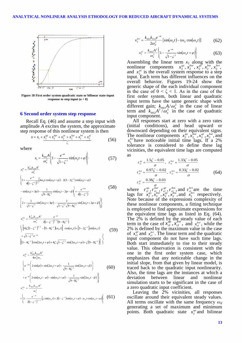
qsx2 , bsix2 , and qix2 are the contributions of the linear, quadratic, and bilinear components in the system behavior. Assembling these components together presents the overall response. To show each component’s effect on the overall behavior, the generic shape of each term is individually visualized as shown in Figure 17 and Figure 18 in the case of a < 0. Both linear and quadratic input components have the same mathematical structure except for the steady gain as shown in Figure 17. Although the normalized state quadratic and bilinear components have different mathematical

Ashraf Omran and Brett Newman

12

structure, both yield the same generic shape as shown in Figure 18 but with different parameters.

All responses start at zero and head upward. The initial slope of the normalized linear and input bilinear terms is tan(υ) = a, while both the normalized state quadratic and bilinear terms have a zero initial slope. This observation indicates that both state quadratic and bilinear terms have no influence on the initial rate in which the system behaves for any input excitation. The initial rate 0x is a function of the ratio between the linear coefficient k01 and the quadratic input coefficient k02 in addition to the input amplitude A. For example, if input quadratic coefficient k02 has a negative sign and the coefficient k01 has a positive sign, the total initial rate is then less than the expected one from the linear analysis and there may be an undershoot phenomena that appears in the case when the input quadratic coefficient k02 is more dominant or at a high input amplitude A.

Both the state quadratic and bilinear responses have a noticeable lag. The duration of lag in the state quadratic term is longer than in the case of the bilinear term, but its transient rise is steeper. Thus, the quadratic kernel has zero edges and the bilinear kernel has non-zero edges. Referring to these two lags as qs

rl and bsi

rl , if 2% is considered as the required threshold to leave the vicinity of such a lag, then these two lags are approximately found to be 0.45/|a| and 0.2/|a|. Note that the quadratic and bilinear step responses include a ramp function multiplied by an exponential function, which sets hurdles in computing their lag times analytically; a reason for which numerical fitting is considered. These time lags are the instances at which a deviation between linear and nonlinear simulation starts to be significant in the case of a zero input quadratic coefficient, which is frequently observed in aircraft applications.

The deviation between linear and nonlinear responses can be positive or negative depending on the difference in signs between the linear coefficient and both the qs

x2 and bsix2 coefficients. This deviation widens due to an increase in the slopes of the state quadratic and bilinear terms, after the two terms exit from their lag vicinity. This increasing slope reaches a maximum at time qs

rm = 1.6/|a| and bsi

rm = 1/|a| for qs

x2 and bx2respectively, which are computed

using numerical fitting. After reaching these maximum slopes, a rapid decrease in each term’s rate leads to an offset difference between the linear and nonlinear responses. Sequentially, each term settles to its steady gain at equivalent

settling times lrs = qi

rs = 4/|a| in the case of the linear and input quadratic terms, qs

rs = 6.6/|a| in the case of the state quadratic term, and bsi

rs = 5.8/|a| in the case of the bilinear term. The overall response settles at

a

kA

a

kkA

aa

kkA

a

Akxss

02

2

2

1101

2

2

20

2

01

2

01 (55)

The time for reaching this steady value depends on the ratio between the coefficients of each term and the input amplitude. For example, if the system has only a state quadratic nonlinearity and this term has a negative sign, which means negative qs

x2 , the settling time in this case is less than the linear settling time, since the system settles before the steady value of the linear term. Such observation reveals that nonlinearity sometimes may improve the system behavior.

The resultant analytical Volterra-based model for the first order SDOF system illuminates many of the nonlinearities usually observed in experimental and numerical results such as the amplitude-dependency response, or how the system becomes non-homogenous with increasing input amplitude. Hence, changing the amplitude not only changes the steady value of the output, but also changes the shape through which the system reaches this steady value. Also, the linear coefficient a not only controls the stability of the system, but also controls the system nonlinearity strength. For example, in the case of a highly damped system, if the system is weakly nonlinear or the nonlinear terms are neglected compared to the linear terms, the system then behaves close to a linear one. On the other hand, if the system lacks sufficient damping, the nonlinearity cannot be neglected even though the nonlinear terms are small. Thus, the low stability gain a increases the significance of the second order quadratic state kernel and instability arises possibly before the condition a = 0.

Figure 17 First order system linear or quadratic input response to

step input (a < 0)

13

ANALYTICAL NONLINEAR ANALYSIS ETHODOLOGY FOR REDUCED AIRCRAFT DYNAMICAL SYSTEMS

Figure 18 First order system quadratic state or bilinear state-input

response to step input (a < 0)

6 Second order system step response

Recall Eq. (46) and assume a step input with amplitude A excites the system, the approximate step response of this nonlinear system is then

2

2222221

x

qibribpiqrbprqp xxxxxxxx (56)

where

teAk

x d

t

n

sin1

122

0011

(57)

ˆ22sin891

1 32sin

1

12

14ˆ2sin

89

13sin

sin)23(2cos414

1

222

2

2

2

2

23

2

6

2

200

2

0012

tt

ett

ttte

Akkx

dd

t

dd

ddd

t

n

qs

(58)

892sin142cos43

1

sin 23cos 89116

8912

222

2

222/32

22/325

2

110

2

001

2

tt

e

ttt

eAkkx

dd

t

ddd

t

n

bsr

(59)

ˆ2sin89

1sinsin2

ˆ2sin89

12sinsin2

4

2

2

2

3

2

020

2

001

2

ttte

tte

Akkx

ddd

t

dd

t

nd

qr

(60)

tttte

Akkx

dddd

t

n

bsi

cossin12sin

12

1 2

2/32

4

2

101001

2

(61)

tttekk

x ddd

d

tbri

cossin2 3

011001

2

(62)

teAk

x d

t

n

qi sin1

122

2

002

2

(63)

Assembling the linear term x1 along with the nonlinear components ,,,,, 22222

bribsiqrbsrqs xxxxx and qix2 is the overall system response to a step input. Each term has different influences on the overall behavior. Figures 19-24 show the generic shape of the each individual component in the case of 0 < ζ < 1. As in the case of the first order system, both linear and quadratic input terms have the same generic shape with different gain; 2

001 / nAk in the case of linear term and 22

002 / nAk in the case of quadratic input component.

All responses start at zero with a zero rates (initial conditions), and head upward or downward depending on their equivalent signs. The nonlinear components ,,,, 2222

bsiqrbsrqs xxxx and brix2 have noticeable initial time lags. If a 2%

tolerance is considered to define these lag vicinities, the equivalent time lags are computed as

0.0338.0

0.0233.0 ,

0.0297.0

0.051.33 ,

0.051.5

qr

rl

bri

rl

bsi

rl

bsr

rl

qs

rl

(64)

where ,,,, bsi

rl

qr

rl

bsr

rl

qs

rl and bri

rl are the time lags for ,,,, 2222

bsiqrbsrqs xxxx and brix2 respectively. Note because of the expressions complexity of these nonlinear components, a fitting technique is employed to find approximate expressions for the equivalent time lags as listed in Eq. (64). The 2% is defined by the steady value of each term in the case of ,, bsr

rl

qs

rl xx and bsi

rlx , while the 2% is defined by the maximum value in the case of qr

rlx and bri

rlx . The linear term and the quadratic input component do not have such time lags. Both start immediately to rise to their steady value. This observation is consistent with the one in the first order system case, which emphasizes that any noticeable change in the initial slope, from that given by linear model, is traced back to the quadratic input nonlinearity. Also, the time lags are the instances at which a deviation between linear and nonlinear simulation starts to be significant in the case of a zero quadratic input coefficient.

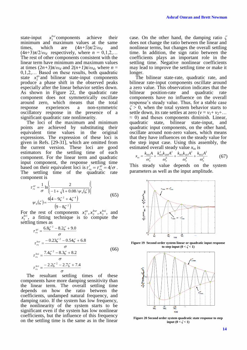
Leaving the 2% vicinities, all responses oscillate around their equivalent steady values. All terms oscillate with the same frequency ωd generating a set of maximum and minimum points. Both quadratic state qsx2 and bilinear

Ashraf Omran and Brett Newman

14

state-input bsix2components achieve their

minimum and maximum values at the same times, which are (4n+5)π/2/ωd and (4n+3)π/2/ωd respectively, where n = 0,1,2,… The rest of other components consistent with the linear term have minimum and maximum values at times (2n+3)π/ωd and 2(n+1)π/ωd, where n = 0,1,2,… Based on these results, both quadratic state qsx2

and bilinear state-input components produce a phase shift in the observed peaks especially after the linear behavior settles down. As shown in Figure 22, the quadratic rate component does not symmetrically oscillate around zero, which means that the total response experiences a non-symmetric oscillatory response in the presence of a significant quadratic rate nonlinearity.

The loci of the maximum and minimum points are achieved by substituting their equivalent time values in the original expressions. The expression of these loci is given in Refs. [29-31], which are omitted from the current version. These loci are good estimators for the settling time of each component. For the linear term and quadratic input component, the response settling time based on their equivalent loci is 4 qi

rs

l

rs . The settling time of the quadratic rate component is

2

42

9

9

89

4946

/08.011

2ln

1

qr

rs

(65)

For the rest of components ,,, 222

bsibsrqs xxx andbrix2 , a fitting technique is to compute the

settling times as

4.77.22.2

2.83.84.7

8.654.023.0

0.92.88.6

2

2

2

2

bri

rs

bsi

rs

bsr

rs

qs

rs

τ (66)

The resultant settling times of these components have more damping sensitivity than the linear term. The overall settling time depends on how the ratio between the coefficients, undamped natural frequency, and damping ratio. If the system has low frequency, the nonlinearity of the system starts to be significant even if the system has low nonlinear coefficients, but the influence of this frequency on the settling time is the same as in the linear

case. On the other hand, the damping ratio δ does not change the ratio between the linear and nonlinear terms, but changes the overall settling time. In addition, the sign ratio between the coefficients plays an important role in the settling time. Negative nonlinear coefficients may lead to improve the settling time or make it longer.

The bilinear state-rate, quadratic rate, and bilinear rate-input components oscillate around a zero value. This observation indicates that the bilinear position-rate and quadratic rate components have no influence on the overall response’s steady value. Thus, for a stable case δ > 0, when the total system behavior starts to settle down, its rate settles at zero (v = v1+ v2+… ≈ 0) and theses components diminish. Linear, quadratic state, bilinear state-input, and quadratic input components, on the other hand, oscillate around non-zero values, which means that they have influences on the steady value for the step input case. Using this assembly, the estimated overall steady value xss is

2

2

002

4

2

101001

6

2

200

2

001

2

001

nnnn

ss

AkAkkAkkAkx

(67)

This steady value depends on the system

parameters as well as the input amplitude.

Figure 19 Second order system linear or quadratic input response

to step input (0 < ζ < 1)

Figure 20 Second order system quadratic state response to step

input (0 < ζ < 1)

15

ANALYTICAL NONLINEAR ANALYSIS ETHODOLOGY FOR REDUCED AIRCRAFT DYNAMICAL SYSTEMS

Figure 21 Second order system bilinear state-rate response to step

input (0 < ζ < 1)

Figure 22 Second order system quadratic rate response to step

input (0 < ζ < 1)

Figure 23 Second order system bilinear state-input response to step

input (0< ζ < 1)

Figure 24 Second order system bilinear rate-input response to step

input (0 < ζ < 1)

7 Low order motion examples

In this Section, numerical examples of surge and pitch motions are presented to show the capability of the developed Volterra-based model to understand and predict aircraft behavior. For each motion, the trim values of the total nonlinear aircraft model are computed at certain operating conditions. These conditions are selected to represent the behavior of the aircraft near the boundaries of the flight envelope. The low order flight systems are then extracted from the overall model. These low order systems still have the aerodynamic-propulsive coefficients represented by look-up tables. After that, the finite difference technique generates both first and second order stability and control derivatives around the previously considered operating conditions. These derivatives are passed to linear-based and Volterra-based models, while the look-up tables are used for the nonlinear simulation.

In the surge motion example, consider the aircraft flies levelly at an altitude Ho = 10 kft with a constant total velocity Vo = 300 ft/s. The required angle of attack and elevator deflection to lift the aircraft and balance the pitching moment are αo = 15.85 deg and δeo = -11.07 deg, while the required thrust is generated by adjusting the throttle deflection to δtho = 28%. These state and input values are computed using the trim subroutine of F-16 full model in a rectilinear motion. Recall equation (13) and use the finite difference to calculate the derivatives at this flight condition, the equivalent surge equation of motion is

104.06

104.5744.130.0285

11

200110

3-

2-5

th

k

k

th

kka

V

VVV

(68)

In Eq. (68), the quadratic throttle deflection is zero (k02 = 0). Thus, in F-16 engine model, the thrust is linearly related to the throttle deflection.

The surge motion’s first kernel is an exponential function starts at k01 = 13.44 and heads downward with an angle υ = arctan(a) = 1.6 deg reaching zero at time infinity. The required time to settle this first kernel inside a 2% band is s 4.140||/4 al

ks (see Eq. (37) ). The surge motion’s second kernel has two components: quadratic velocity component qsh2

and bilinear velocity-throttle component bsih2.

The linear term a (k10 = -0.0285 1/s) has a relatively low value indicating that the quadratic component qsh2

is more dominant than the bilinear component bsih2

according to Eq. (35). Thus, the quadratic component is proportional

Ashraf Omran and Brett Newman

16

to akk /2

0120 = 0.29 ft/s/rad

2, while the bilinear

component is proportional to k11k01 = 0.0273 ft/s/rad

2. This fact makes the shape of the

second kernel look close to the quadratic state kernel shape in Figure 4. The second kernels’ components settle at about the same time:

bsi

ks

qs

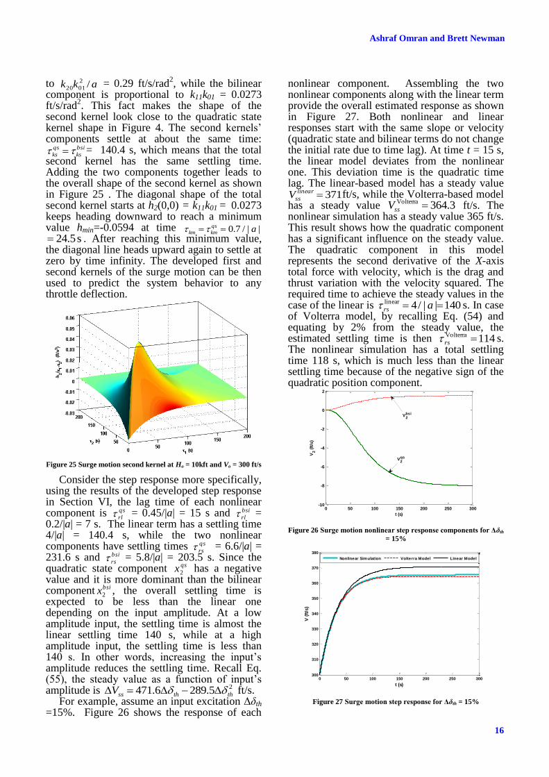
ks = 140.4 s, which means that the total second kernel has the same settling time. Adding the two components together leads to the overall shape of the second kernel as shown in Figure 25 . The diagonal shape of the total second kernel starts at h2(0,0) = k11k01 = 0.0273 keeps heading downward to reach a minimum value hmin=-0.0594 at time

||/7.0 aqs

kmkm s 5.24 . After reaching this minimum value,

the diagonal line heads upward again to settle at zero by time infinity. The developed first and second kernels of the surge motion can be then used to predict the system behavior to any throttle deflection.

Figure 25 Surge motion second kernel at Ho = 10kft and Vo = 300 ft/s

Consider the step response more specifically, using the results of the developed step response in Section VI, the lag time of each nonlinear component is qs

rl = 0.45/|a| = 15 s and bsi

rl =

0.2/|a| = 7 s. The linear term has a settling time 4/|a| = 140.4 s, while the two nonlinear components have settling times qs

rs = 6.6/|a| =

231.6 s and bsi

rs = 5.8/|a| = 203.5 s. Since the quadratic state component qsx2 has a negative value and it is more dominant than the bilinear component bsix2 , the overall settling time is expected to be less than the linear one depending on the input amplitude. At a low amplitude input, the settling time is almost the linear settling time 140 s, while at a high amplitude input, the settling time is less than 140 s. In other words, increasing the input’s amplitude reduces the settling time. Recall Eq. (55), the steady value as a function of input’s amplitude is 25.2896.471 ththssV

ft/s.

For example, assume an input excitation Δδth

=15%. Figure 26 shows the response of each

nonlinear component. Assembling the two nonlinear components along with the linear term provide the overall estimated response as shown in Figure 27. Both nonlinear and linear responses start with the same slope or velocity (quadratic state and bilinear terms do not change the initial rate due to time lag). At time t = 15 s, the linear model deviates from the nonlinear one. This deviation time is the quadratic time lag. The linear-based model has a steady value

371linear

ssV ft/s, while the Volterra-based model has a steady value 3.364Volterra ssV ft/s. The nonlinear simulation has a steady value 365 ft/s. This result shows how the quadratic component has a significant influence on the steady value. The quadratic component in this model represents the second derivative of the X-axis total force with velocity, which is the drag and thrust variation with the velocity squared. The required time to achieve the steady values in the case of the linear is 140||/4linear ars s. In case of Volterra model, by recalling Eq. (54) and equating by 2% from the steady value, the estimated settling time is then 114Volterra rs s. The nonlinear simulation has a total settling time 118 s, which is much less than the linear settling time because of the negative sign of the quadratic position component.

Figure 26 Surge motion nonlinear step response components for Δδth

= 15%

Figure 27 Surge motion step response for Δδth = 15%

0 50 100 150 200 250 300-10

-8

-6

-4

-2

0

2

t (s)

V2 (

ft/s

)

Vqs2

Vbsi2

0 50 100 150 200 250 300300

310

320

330

340

350

360

370

380

t (s)

V (

ft/s

)

Nonlinear Simulation Volterra Model Linear Model

17

ANALYTICAL NONLINEAR ANALYSIS ETHODOLOGY FOR REDUCED AIRCRAFT DYNAMICAL SYSTEMS

The second example represents the pitch motion at an altitude Ho = 40 kft and total velocity Vo = 530 ft/s. For a rectilinear motion, the computed trimming variables are θo = αo = 15.6 deg, δeo = -2.6 deg, and δtho = 98.8%. Using the finite difference technique, the reduced pitch equations of motion, equivalent to Eq. (15), are

2

2

002101110

200001010100

0.001429.016.0

05.115.336.079.0

e

k

e

kk

k

e

kkk

q

qq

q

(69)

In Eq. (69), the quadratic rate coefficient k020 = 0 and the bilinear rate-input coefficient k011 = 0. Thus, both plunge force and pitch moment coefficients are linear related to the pitch rate q with a zero correlation to the elevator deflection δe. The pitch motion model has a damping ratio δ = 0.2, damping factor σ = 0.18 1/s, undamped natural frequency ωn = 0.89 rad/s, and damped natural frequency ωd = 0.87 rad/s. The first kernel starts at zero with a negative slope and keeps oscillating zero with a frequency ωd = 0.87 rad/s. The amplitude of this oscillation decreases with time and settles inside a 2% band of the gain |k001/ ωn| = 3.45 at time ||/4 l

ks 22.2 s. The second kernel has four components. Based on Eqs. (40-45), the influence of each component on the total second kernel, from highest to lowest, is: quadratic state component

qsh2 (with a weight 42

001200 2/ dkk = 6.86), bilinear state-rate component bsrh2

(with a weight 232

001110 12/ dkk = 1.18), bilinear state-input component bsih2

(with a weight 2

001101 2/ dkk = -0.59), and quadratic input component qih2

(with a weight dk /002

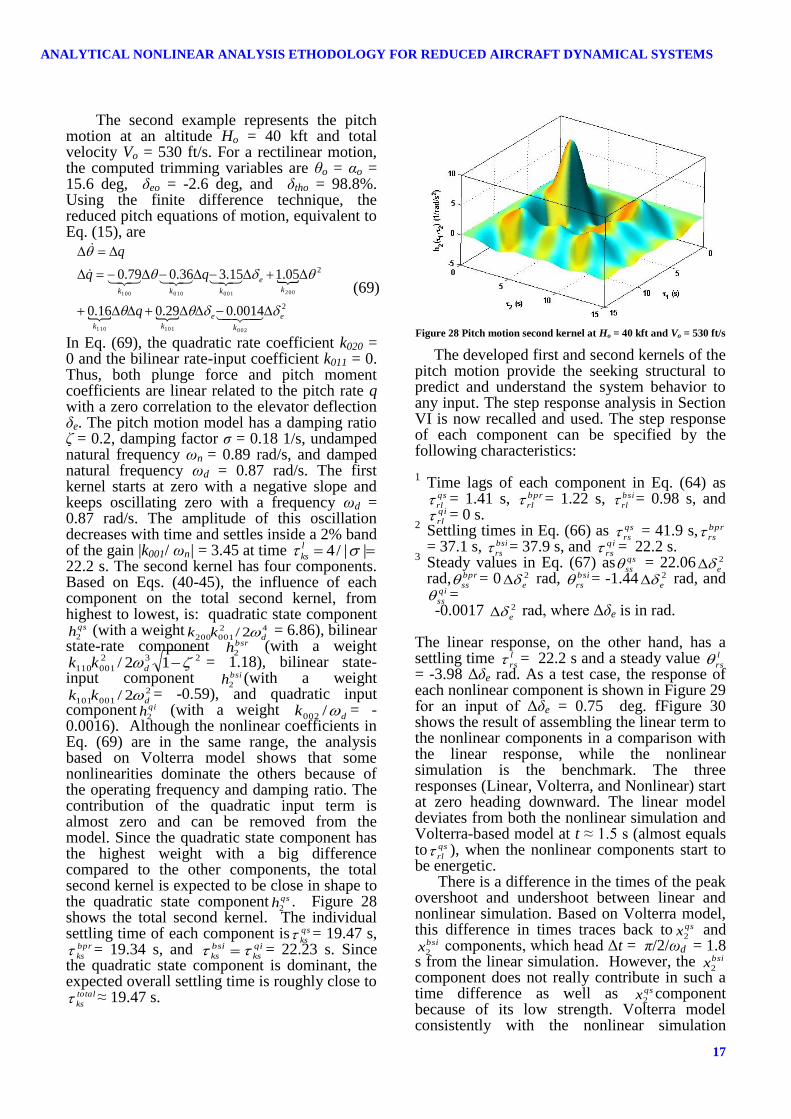
= -0.0016). Although the nonlinear coefficients in Eq. (69) are in the same range, the analysis based on Volterra model shows that some nonlinearities dominate the others because of the operating frequency and damping ratio. The contribution of the quadratic input term is almost zero and can be removed from the model. Since the quadratic state component has the highest weight with a big difference compared to the other components, the total second kernel is expected to be close in shape to the quadratic state component qsh2

. Figure 28 shows the total second kernel. The individual settling time of each component is qs

ks = 19.47 s, bpr

ks = 19.34 s, and qi

ks

bsi

ks = 22.23 s. Since the quadratic state component is dominant, the expected overall settling time is roughly close to

total

ks ≈ 19.47 s.

Figure 28 Pitch motion second kernel at Ho = 40 kft and Vo = 530 ft/s

The developed first and second kernels of the pitch motion provide the seeking structural to predict and understand the system behavior to any input. The step response analysis in Section VI is now recalled and used. The step response of each component can be specified by the following characteristics:

1 Time lags of each component in Eq. (64) as

qs

rl = 1.41 s, bpr

rl = 1.22 s, bsi

rl = 0.98 s, and qi

rl = 0 s. 2 Settling times in Eq. (66) as qs

rs = 41.9 s, bpr

rs= 37.1 s, bsi

rs = 37.9 s, and qi

rs = 22.2 s. 3 Steady values in Eq. (67) as qs

ss = 22.06 2

erad, bpr

ss = 0 2

e rad, bsi

rs = -1.44 2

e rad, and qi

ss = -0.0017 2

e rad, where Δδe is in rad.

The linear response, on the other hand, has a settling time l

rs = 22.2 s and a steady value l

rs= -3.98 Δδe rad. As a test case, the response of each nonlinear component is shown in Figure 29 for an input of Δδe = 0.75 deg. fFigure 30 shows the result of assembling the linear term to the nonlinear components in a comparison with the linear response, while the nonlinear simulation is the benchmark. The three responses (Linear, Volterra, and Nonlinear) start at zero heading downward. The linear model deviates from both the nonlinear simulation and Volterra-based model at t ≈ 1.5 s (almost equals to qs

rl ), when the nonlinear components start to be energetic.

There is a difference in the times of the peak overshoot and undershoot between linear and nonlinear simulation. Based on Volterra model, this difference in times traces back to qsx2

and bsix2

components, which head Δt = π/2/ωd = 1.8 s from the linear simulation. However, the bsix2

component does not really contribute in such a time difference as well as qsx2

component because of its low strength. Volterra model consistently with the nonlinear simulation

Ashraf Omran and Brett Newman

18

provides the times of the first three overshoot peaks at: 6.76s, 13.67s, and 20.47 s. The linear model, on the other hand, provides these times at: 7.22s, 14.43s, and 21.64s. It is clear how the time difference propagates with time to reach a phase shift 90 deg by the third cycle. The equivalent percentage maximum overshoots at these times are: [7.5% 3.2% 1.5%] based on the linear model and [8.0% 3.9% 2.1%] based on the Volterra model, which is the same as the nonlinear simulation. The differences in estimating the maximum overshoot values and their equivalent times emphasize that developed analytical models based on Volterra theory provides a better tool in predicting the transient response of the aircraft especially for tracking applications when these differences are a matter of concern. The developed analytical Volterra model not only proves the capability to render the transient response but also the steady response as volterra

ss 12.79 deg compared to

linear

ss 12.6 deg from the linear model with an error 7%. The estimated settling time to reach this value is 4.19linear

st s and 6.24linear

st s.

Figure 29 Pitch motion nonlinear step response components for Δδe

= 0.75 deg

fFigure 30 Pitch motion step response for Δδe = 0.75 deg

8 Conclusion

A procedure to analytically assemble the constituents of the dynamic response of simple low order nonlinear systems based on multi-dimensional convolution expansion theory has been offered. The procedure provides closed-form expressions for the convolution integral kernels, which in turn lead to expressions for the time response for a step input. The explicit nature of the relational expressions allow cause-and-effect insights between nonlinearities present in the state space model and corresponding response traits. The procedure facilitates system prediction before employing computer simulation and/or system analysis after computer simulation. At this point in time, the procedure has only been developed for first and second order single degree of freedom systems. Expanding this framework to multi-axis motions is of future interest. Application to single state and dual state uni-axis aircraft motion exposed the source of differences between nonlinear and linear responses, specifically initial departure time, maximum and steady offsets, differences in settling times, and oscillation frequency and phasing shifts

References

1. Liebst, S. and Nolan, C., “A Simplified Wing Rock

Prediction Method,” AIAA-1993-3662, Atmospheric

Flight Mechanic Conference, Monterey, CA, August

1993.

2. Jahnke, C. and Culick, C., “Application of

Bifurcation Theory to the High-Angle-of-Attack

Dynamics of the F-14,” Journal of Aircraft, Vol. 31,

No. 1, January-February 1994, pp. 26-34.

3. Ananthkrishnan, N. and Sudhakar, K.,

“Characterization of Periodic Motions in Aircraft

Lateral Dynamics,” Journal of Guidance, Control,

and Dynamics, Vol. 19, No. 3, May-June 1996, pp.

680-685.

4. Nandan , S., “Applications of Bifurcation Methods to

F-18 HARV Open-Loop Dynamics in Landing

Configuration,” Defense Science Journal, Vol. 52,

No. 2, April 2002, pp. 103-115.

5. Go, T. and Ramnath, R., “Analytical Theory of

Three-Degree-of-Freedom Aircraft Wing Rock,”

Journal of Guidance, Control, and Dynamics Vol. 27,

No. 4, July-August 2004, pp. 657-664.

6. James, C. and Raman, M., “Bifurcation Analysis of

Nonlinear Aircraft Dynamics,” Journal of Guidance,

Control, and Dynamics, Vol. 5, No. 5, September-

October 1982, pp. 529-536.

7. Raghavendra, P., Sahai, T., Kumar, P., Chauhan, M.,

and Ananthkrishnan, N., “Aircraft Spin Recovery,

with and without Thrust Vectoring, Using Nonlinear

0 5 10 15 20 25 30 35-0.2

-0.1

0

0.1

0.2

0.3

0.4

0.5

0.6

0.7

t (s)

2 (

deg

)

2qs

2bsr

2bsi

2qi

0 2 4 6 8 10 12 14 16 18 2011

11.5

12

12.5

13

13.5

14

14.5

15

15.5

16

t (s)

(

deg

)

Nonlinear Simulation

Volterra Model

Linear Model

19

ANALYTICAL NONLINEAR ANALYSIS ETHODOLOGY FOR REDUCED AIRCRAFT DYNAMICAL SYSTEMS

Dynamic Inversion,” Journal of Aircraft, Vol. 42,

No. 6, November-December 2005, pp. 1492-1503.

8. Mehra, K., Woburn, M., Prasanth, K., and Woburn,

M., “Bifurcation and Limit Cycle Analysis of

Nonlinear Pilot Induced Oscillations,” AIAA

Atmospheric Flight Mechanics Conference, Boston,

MA, August 1998.

9. Newman, B., “Dynamics and Control of Limit

Cycling Motions in Boosting Rockets,” Journal of

Guidance, Control, and Dynamics, Vol. 18, No. 2,

March-April 1995, pp. 280-286.

10. Duda, H., “Effects of Rate Limiting Elements in

Flight Control Systems a New PIO-Criterion,” AIAA

Guidance, Navigation and Control Conference,

Baltimore, MD, August 1995.

11. Klyde, H., McRuer, T., and Myers, T., “PIO Analysis

with Actuator Rate Limiting,” AIAA Atmospheric

Flight Mechanics Conference, San Diego, CA, July

1996.

12. Go, T., “Lateral-Directional Aircraft Dynamics under

Static Moment Nonlinearity,” Journal of Guidance,

Control, and Dynamics, Vol. 32, No. 1, January–

February 2009, pp. 305-309.

13. Mehra, K., Washburn, B., and Carrol, V., “A Study

of the Application of Singular Perturbation Theory,”

NASA CR-3167, 1979.

14. Volterra, V., “Theory of Functionals and of Integral

and Integro-Differential Equations,” Dover, New

York, 1958.

15. Rugh, J. W., “Nonlinear System Theory: The

Volterra/Wiener Approach,” John Hopkins

University Press, 1981.

16. Wiener, N., “Response of a Nonlinear Device Noise,”

Massachusetts Institute of Technology Radiation

Laboratory, Technical Report No. 165, Cambridge,

MA, 1942.

17. Brilliant, M., "Theory of the Analysis of Nonlinear

Systems," Massachusetts Institute of Technology

Radiation Laboratory, Technical Report No. 345,

Cambridge, MA, 1958.

18. George, D., "Continuous Nonlinear Systems,"

Massachusetts Institute of Technology Radiation

Laboratory, Technical Report No. 355, 1959.

19. Mohler, R. R., “Nonlinear Stability and Control

Study of Highly Maneuverable High Performance

Aircraft,” NASAOSU-ECE Report No. 91-01, 1991.

20. Stalford, H., Baumann, W., Garrett, E. F., and

Herman, T., “Accurate Modeling of Nonlinear

System Using Volterra Series Submodels,” AACC

American Control Conference, Vol. 2, Minneapolis,

MN, July 1987, pp. 886-891.

21. Suchomel, C. F., “Nonlinear Flying Qualities - One

Approach,” AIAA Aerospace Sciences Meeting,

Reno, NV, January 1987.

22. Omran, A. and Newman, B., “Global Aircraft

Dynamics Using Piecewise Volterra Kernels,” AIAA

Atmospheric Flight Mechanics Conference,

Honolulu, HI, August 2008.

23. Omran, A. and Newman, B., “Piecewise Global

Volterra Nonlinear Modeling and Characterization

for Aircraft Dynamics,” Journal of Guidance,

Control, and Dynamics, Vol. 32, No. 3, May-June

2009, pp. 749-759.

24. Nguyen, L., Ogburn, M., Gilbert, W., Kibler, K.,

Brown, P., and Deal, P., “Simulator Study of

Stall/Post-Stall Characteristics of a Fighter Airplane

with Relaxed Longitudinal Static Stability,” NASA

TP-1538, 1979.

25. Stevens, B. and Lewis, F., Aircraft Control and

Simulation, John Wiley & Sons, New York, 1992.

26. Franz, M. and Scholkopf, B., “A Unifying View of

Wiener and Volterra Theory and Polynomial Kernel

Regression,” Neural Computation, Vol. 18, No. 12,

December 2006, pp. 3097-3118.

27. Gilbert, E., “Functional Expansions for the Response

of Nonlinear Differential Systems,” IEEE

Transactions on Automatic Control, Vol. 22, No. 6,

December 1977, pp. 909-921.

28. Nguyen, T., Whipple, D., and Brandon, J., “Recent

Experience of Unsteady Aerodynamic Effect on

Flight Dynamics at High Angle of Attack,” AGARD

Conference Proceedings, Symposium on Unsteady

Aerodynamics-Fundamentals and Applications to

Aircraft Dynamics, Gottingen, Germany, May 1985.

29. Omran, A., and Newman, B., “On Dynamical

Assembly of Nonlinear Uniaxial Atmospheric Flight

Mechanics,” Proceedings of AIAA Atmospheric

Flight Mechanics Conference, Chicago, Illinois,

August 2009.

30. Omran A. and Newman B., “Analytical Response for

the Prototypic Nonlinear Mass-Spring-Damper

System,” ESDA2010 Proceedings of the ASME2010

10th Biennial Conference on Engineering System

Design and Analysis, Istanbul, Turkey, July 12-14,

2010.

31. Omran A. and Newman B., “Nonlinear Cause-Effect

Analysis for a Second Order System using Volterra

Kernels,”ACC2010, IEEE American Control

Conference, Baltimore, Maryland, June 30 - July 2,

2010.

Copyright Statement

The authors confirm that they, and/or their company or

organization, hold copyright on all of the original material

included in this paper. The authors also confirm that they

have obtained permission, from the copyright holder of

any third party material included in this paper, to publish

it as part of their paper. The authors confirm that they

give permission, or have obtained permission from the

copyright holder of this paper, for the publication and

distribution of this paper as part of the ICAS2010

proceedings or as individual off-prints from the

proceedings.