HAL Id: hal-01401907https://hal.archives-ouvertes.fr/hal-01401907

Submitted on 24 Nov 2016

HAL is a multi-disciplinary open accessarchive for the deposit and dissemination of sci-entific research documents, whether they are pub-lished or not. The documents may come fromteaching and research institutions in France orabroad, or from public or private research centers.

L’archive ouverte pluridisciplinaire HAL, estdestinée au dépôt et à la diffusion de documentsscientifiques de niveau recherche, publiés ou non,émanant des établissements d’enseignement et derecherche français ou étrangers, des laboratoirespublics ou privés.

Distributed under a Creative Commons Attribution| 4.0 International License

Analytical modeling of synthetic fiber ropes subjected toaxial loads. Part I: A new continuum model for

multilayered fibrous structuresSeyed Reza Ghoreishi, Patrice Cartraud, Peter Davies, Tanguy Messager

To cite this version:Seyed Reza Ghoreishi, Patrice Cartraud, Peter Davies, Tanguy Messager. Analytical modeling ofsynthetic fiber ropes subjected to axial loads. Part I: A new continuum model for multilayered fi-brous structures. International Journal of Solids and Structures, Elsevier, 2007, 44 (9), pp.2924-2942.�10.1016/j.ijsolstr.2006.08.033�. �hal-01401907�

Analytical modeling of synthetic fiber ropes subjectedto axial loads. Part I: A new continuum model

for multilayered fibrous structures

Seyed Reza Ghoreishi a, Patrice Cartraud a, Peter Davies b, Tanguy Messager c

a Institut de recherche en Genie civil et Mecanique (GeM), Ecole Centrale de Nantes, 1, Rue de la Noe, BP92101,

44321 Nantes Cedes 03, Franceb IFREMER, Materials and Structures group BP70, 29280 Plouzane, France

c Universite de Nantes, Nantes Atlantique Universites, Institut de recherche en Genie civil et Mecanique (GeM),

Ecole Centrale de Nantes, BP92101, 44321 Nantes, France

Synthetic fiber ropes are characterized by a very complex architecture and a hierarchical structure. Considering the fiberrope architecture, to pass from fiber to rope structure behavior, two scale transition models are necessary, used insequence: one is devoted to an assembly of a large number of twisted components (multilayered), whereas the second issuitable for a structure with a central straight core and six helical wires (1 + 6). The part I of this paper first describesthe development of a model for the static behavior of a fibrous structure with a large number of twisted components. Testswere then performed on two different structures subjected to axial loads. Using the model presented here the axial stiffnessof the structures has been predicted and good agreement with measured values is obtained. A companion paper presents thesecond model to predict the mechanical behavior of a 1 + 6 fibrous structure.

Keywords: Fiber rope; Yarn; Aramid; Multilayered structures; Analytical model; Testing

1. Introduction

Synthetic fiber rope mooring systems, which are often composed of steel chain at the ends and a centralsynthetic fiber rope, are increasingly finding applications as offshore oil exploration goes to deeper sites. Pre-vious researchers have shown that such mooring lines provide numerous advantages over steel mooring lines

1

(steel wire ropes and chains), particularly in deep water applications for which the large self-weight of steellines is prohibitive (Beltran and Williamson, 2004; Foster, 2002). It is therefore essential to be able to modelthe mechanical behavior of very long synthetic mooring lines in order to reduce the need for expensive testsunder varying parameters and operating conditions.

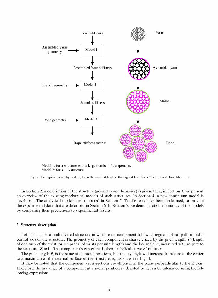
Large synthetic fiber ropes are assemblies of millions of fibers and characterized by a very complex archi-tecture and a hierarchical structure in which the base components (fiber or yarn) are modified by twistingoperations. This structure is then a base component for the next higher structure. Its hierarchical structureleads to the hierarchical approach where the top is the fiber rope and the bottom is the base components, withseveral different types of elements between the base component and the fiber rope, i.e. yarn, assembled yarnand strand. Fig. 1 illustrates this hierarchical structure.

Considering the fiber rope architecture, it consists of two different types of structure: one is a structure witha central straight core and six helical components (1 + 6), whereas the second is an assembly of a large numberof twisted components (multilayered), see Fig. 2. So to pass from fiber to rope structure, two scale transitionmodels are necessary, used in sequence. The results of the model at each level can be used as input data for themodel at the next higher level. Use of this approach from the lowest level, at which mechanical properties aregiven as input, to the highest level of the rope determines the rope properties. Based on this strategy, the tran-sition models can be used to analyze synthetic fiber ropes of complex cross-section. Fig. 3 shows the typicalhierarchy ranking from the smallest level to the highest level for a 205 ton break load fiber rope.

The focus of this paper is the modeling of the static behavior of a fibrous structure with a large number oftwisted components subjected to axial loads, starting from the mechanical behavior of the base component,and the geometric description of the rope structure.

Cross section A-A

A A

Yarn

Fiber

Strand

Assembled yarn

Fig. 1. Synthetic fiber rope structure. (a) Fiber robe with 1 + 6 strands and (b) construction of a strand.

Fig. 2. Cross-section of a synthetic fiber rope (205 ton break load); the rope represents a 1 + 6 structure, core and strands are assemblies ofa large number of twisted components.

2

In Section 2, a description of the structure (geometry and behavior) is given, then, in Section 3, we presentan overview of the existing mechanical models of such structures. In Section 4, a new continuum model isdeveloped. The analytical models are compared in Section 5. Tensile tests have been performed, to providethe experimental data that are described in Section 6. In Section 7, we demonstrate the accuracy of the modelsby comparing their predictions to experimental results.

2. Structure description

Let us consider a multilayered structure in which each component follows a regular helical path round acentral axis of the structure. The geometry of each component is characterized by the pitch length, P (lengthof one turn of the twist, or reciprocal of twists per unit length) and the lay angle, a, measured with respect tothe structure Z axis. The component’s centerline is then an helical curve of radius r.

The pitch length P, is the same at all radial positions, but the lay angle will increase from zero at the centerto a maximum at the external surface of the structure, ae, as shown in Fig. 4.

It may be noted that the component cross-sections are elliptical in the plane perpendicular to the Z axis.Therefore, the lay angle of a component at a radial position ri, denoted by ai can be calculated using the fol-lowing expression:

Yarn stiffness

Model 1Assembled yarns

geometry

Model 1Strands geometry

Rope geometry

Assembled Yarn stiffness

Strands stiffness

Rope stiffness matrix

Yarn

Assembled yarn

Strand

Rope

Model 2

Model 1: for a structure with a large number of components.Model 2: for a 1+6 structure.

Fig. 3. The typical hierarchy ranking from the smallest level to the highest level for a 205 ton break load fiber rope.

3

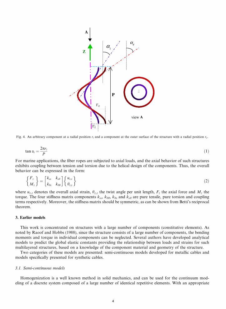
tan ai ¼2pri

Pð1Þ

For marine applications, the fiber ropes are subjected to axial loads, and the axial behavior of such structuresexhibits coupling between tension and torsion due to the helical design of the components. Thus, the overallbehavior can be expressed in the form:

F z

Mz

� �¼

kee keh

khe khh

� �uz;z

hz;z

� �ð2Þ

where uz,z denotes the overall axial strain, hz,z the twist angle per unit length, Fz the axial force and Mz thetorque. The four stiffness matrix components kee, khh, khe and keh are pure tensile, pure torsion and couplingterms respectively. Moreover, the stiffness matrix should be symmetric, as can be shown from Betti’s reciprocaltheorem.

3. Earlier models

This work is concentrated on structures with a large number of components (constitutive elements). Asnoted by Raoof and Hobbs (1988), since the structure consists of a large number of components, the bendingmoments and torque in individual components can be neglected. Several authors have developed analyticalmodels to predict the global elastic constants providing the relationship between loads and strains for suchmultilayered structures, based on a knowledge of the component material and geometry of the structure.

Two categories of these models are presented: semi-continuous models developed for metallic cables andmodels specifically presented for synthetic cables.

3.1. Semi-continuous models

Homogenization is a well known method in solid mechanics, and can be used for the continuum mod-eling of a discrete system composed of a large number of identical repetitive elements. With an appropriate

Fig. 4. An arbitrary component at a radial position ri and a component at the outer surface of the structure with a radial position re.

4

choice of the material parameters, one can accurately represent the global behavior of the real system. Thismethod was first applied to cable modeling by Hobbs and Raoof (1982). It is the orthotropic sheet modelthat has been described in detail by Raoof (1983) and then extended by Raoof and his associates over twodecades.

In this model the classical twisted rod theories for the behavior of helical laid wires has been extended toinclude a set of kinematic compatibility conditions. The individual layer of wires is replaced by an equivalentcylindrical orthotropic sheet, which is assumed to be thin and to be in a plane stress state.

As in the case of composite laminates, four elastic constants are necessary. Two of them are obtaineddirectly from the mechanical properties of the wires. The other two are related to the contact stiffness betweenadjacent wires in the layer. The complete structure is then treated as a discrete set of concentric orthotropiccylinders. The orthotropy axes correspond to those of a fiber composite material in which the fibers have thesame lay angle as the wires in the corresponding layer.

Another semi-continuous model was developed by Blouin and Cardou (1989), and later extended by Jolic-oeur and Cardou (1994, 1996). This also consists of replacing each layer with a cylinder of orthotropic, trans-versely isotropic material. In this model the elastic constants can be used as free, adjustable, parameters, orelse estimated rationally from contact mechanics equations as in the case of the orthotropic sheet model.

Once the cable is modeled using such continuum approach, analytical solutions for elementary loadings canbe derived (Crossley et al., 2003a,b).

These semi-continuous models take into account friction between constituents. However, some elastic con-stants are obtained from contact mechanics, considering layer components have circular cross-section. It canbe seen from Fig. 2 that this is not the case for fiber ropes. Moreover, due to the homogenization process, theaccuracy of this model increases when the number of wires in a given layer increases. Lastly, these models aretedious to use, and since they are non-linear, they require numerical solving.

Despite these limitations, the model of Raoof and Hobbs (1988), briefly presented in Section 3.3, will beapplied here in section 5.

3.2. Synthetic fiber ropes models

In this category the simplest model is that of Hoppe (1991) in which the structure and the components areassumed to be subjected to pure tensile forces, the bending and torsional stiffness for both of them beingneglected. Contact and friction between the components are also neglected, but such an approximation is jus-tified for monotonic axial loading. It should be noted that this analytical model provides only the overall ten-sile behavior.

Leech et al. (1993), presented a more complex quasi-static analysis of fiber ropes and included it in a com-mercial software: fiber rope modeller or FRM (2003). Their analysis is based on the principle of virtual workand can take frictional effects into account. The program computes tension and torque from their dependenceon elongation and twist.

Another model was developed by Rungamornrat et al. (2002), and later extended by Beltran et al. (2003)and Beltran and Williamson (2004). These models are very similar with that of Leech but they have concen-trated on a damage model to take into account the degradation of rope properties as a function of loadinghistory.

Leech’s model appears to be very sophisticated, with an accurate mechanical modeling of the componentsof the fiber ropes behavior and their interactions. Moreover, the cross-section geometry can be described usingdifferent forms of arrangement of components (see Section 3.5). Therefore, Leech’s model can be considered asa reference model, but it requires resolution.

Hereafter, the synthetic fiber ropes models of Hoppe (1991) and Leech et al. (1993) are briefly presented andthen a new continuum model will be developed from the Hoppe’s one to analysis the structure with a largenumber of twisted components.

3.3. Raoof’s model

Raoof and his associates have worked extensively on the behavior of metallic structures with a large num-ber of wires so that the bending moments and torque in individual wires become much less significant than

5

they are in six and seven wire cables (Hobbs and Raoof, 1982; Raoof, 1983; Raoof and Hobbs, 1988; Raoof,1991; Raoof and Kraincanic, 1995a; Raoof and Kraincanic, 1995b). In these studies a great deal of attentionhas been paid to the inter-wire contact phenomena and friction has been taken fully into account. By treatingeach layer of wires as an orthotropic sheet with non-linear properties determined using the mechanical contacttheories and assuming Coulomb friction, it has been possible to establish the stiffness matrix in the presence ofan axial load.

The main features of this model are presented hereafter, in the case of metallic multilayered structure withan isotropic material.

These authors have established a set of non-linear simultaneous equations to analyse the kinematics of eachlayer of wires, providing a set of compatible strains in the anisotropic cylinder with a core (for more details seeRaoof and Hobbs (1988)). The elastic behavior of each orthotropic sheet in the local coordinate system(t,b,n), see Fig. 5, can be expressed in the following matrix form:

ett

ebb

etb

8><>:

9>=>; ¼

S11 S12 0

S12 S22 0

0 0 S66

8><>:

9>=>;

rtt

rbb

rtb

8><>:

9>=>; ð3Þ

where Sij, e and r are the compliance, the strains and stresses referred to the axes of orthotropy parallel andnormal to the wire axes, respectively.

The compliance parallel to the wire axis S11 is straightforward, reflecting the ratio between the sheet areaand the wire area (4/p):

S11 ¼4

pEð4Þ

where E is the Young’s modulus for the wire material, and the coupling term S12 is given by

S12 ¼ �mS11 ð5Þ

where m is Poisson’s ratio.

Fig. 5. Local and global coordinate systems for a layer of wires.

6

The compression compliance, S22, has been expressed as

S22 ¼1

pE4ð1� m2Þ 1

3þ ln

1:25D

P cDð1�m2ÞE

� �1=2

264

375� 2ð1� m2Þ

0B@

1CA ð6Þ

where D is the wire diameter and, Pc is the contact load per unit length on the contact area which is obtainedfrom Hertzian contact theory for the contact of two parallel cylinders. The contact load, Pc, is determinednumerically by using an iterative method.

The shear compliance, S66, is determined from other results of the contact theory (Mindlin, 1949):

S66 ¼S22

1� m1� dl

dlmax

� �1=2

ð7Þ

where dl is the line contact displacement for a given total perturbation in structure axial strain, and dl max is thecorresponding displacement at the onset of full-sliding condition.

The stiffness (or compliance) has been shown to be a function of the amplitude of the load variation aboutthe mean. For small changes of axial force the stiffness is larger than it is for bigger variations. Small changesdo not overcome the inter-wire friction, while larger changes do, causing sliding and a lower effective modulus.

In this study, the stiffness matrix results of this model for two extreme cases are presented: the lower boundor full-slip, correspond to dl = dl max and the upper bound or no-slip for dl = 0.

Once the stiffness matrix of all the layers (for a given axial preload) has been found, in order to obtain thebehavior of the structure, the stiffness matrix of each layer is transformed into the global coordinate system ofthe structure (t 0, b 0, n 0), see Fig. 5, and the summation of the stiffness of all the layers enables the global behav-ior of the structure to be established.

It should be noted that to apply this model to a multilayered fibrous structure, Young’s modulus of thecomponent material is obtained from axial stiffness of components in the direction of their axis, see section4. In addition, Poisson’s ratio, m, according to the volume constant deformation assumption, has been setto 0.5.

3.4. Hoppe’s model

The work of Hoppe (1991) based on purely geometrical considerations, allows a model of behavior of thistype of structure under a simple tensile force to be determined. This model requires the knowledge of the ten-sile properties of the components and the construction parameters of the structure, i.e. the number of layers,the number of components in each layer and the lay angle of each layer. This model is based on the followinghypotheses: the geometry of the structure is multilayered with the helical component having circular section; atthe local and global levels, the base components and the structure work only in traction in the direction oftheir axis (bending and torsion are neglected); the section of the structure remains plane, and perpendicularto its axis after deformation; deformation of the structure is at constant volume; strains and friction effectsdue to contact between components are neglected.

Using these hypotheses, the elongation of each component is determined as a function of those of the struc-ture, and then the axial force in each component is determined. The projection of the force on the structureaxis and summing for all the components enables a closed-form expression for the global behavior (only axialstiffness) of the structure to be established. In section 4, a closed-form analytical solution, for stiffness matrixcomponents, will be developed which is based on Hoppe’s model.

3.5. Leech’s model

Leech et al. (1993) presented a model whose formulation is based on the principle of virtual work to ana-lyze fiber ropes. This model is integrated in a commercial software (FRM, 2003) to predict the behavior ofthe synthetic cables subjected to an axial load. This model differs from Hoppe’s model by the followingaspects: at the global level, the behavior of the structure is characterized by coupling between tension andtorsion phenomena using a 2 · 2 stiffness matrix; friction effects due to contact and the relative motions

7

between components are considered; the geometry of the structure is multilayered, and two extreme ropegeometry descriptions in transverse deformation have been considered: Layered packing geometry andWedge geometry, see Fig. 6.

For layered packing geometry, it is assumed that a bundle of parallel identical components with circularcross-section is twisted in the assembly to form a structure with a core, surrounded by a layer of equallywound components, this layer enclosed by another layer and so on until all the components are used. Eachlayer is a helical structure of many components and each helix has the same pitch length but a different layangle.

For wedge geometry, the components in the same level are allowed to deform transversely and change theirshape to a wedge or truncated wedge. The equivalent helix radius is the radius of the center of area of thewedge. Within each layer the packing factor (PF) is introduced to take into account the presence of the voidsin the layer that can be defined by the ratio of the area of material to the layer cross-sectional area. It can beexpressed by

PF i ¼niAc= cos ai

2priW ið8Þ

where ni, Ac and Wi are the number of components in layer i, component cross-section area and the width ofthe layer i respectively. It should be noted that for a given PF, the width of the layer will be defined and viceversa.

The estimation of the frictional forces that develop between the components in a structure is based on theclassical slip-stick model where the friction force is assumed to develop between two contact surfaces in thedirection opposite to the relative slip of these two surfaces. Six sliding modes have been presented and itwas noted that, for the twisted structure under axial loading, the only significant frictional contribution(and even that is small) comes from the axial sliding mode (Leech et al., 1993; Leech, 2002).

In the present study, FRM software was used to obtain the results for Leech’s model, with the wedge geom-etry option. First, the structure is defined. Essentially, this consists of specifying the number of components ineach layer with the appropriate twist and the nature of the packing at that layer. Second, the dimensional andtensile properties of the components must be provided. Most are single parameters, but the non-linear force–strain relations can be defined in the software by the coefficients of fourth order polynomials. In this study theforce–strain relations were considered linear and derived from test data.

The stiffness matrix is obtained in two steps. First, we let hz,z = 0 and vary the axial strain, uz,z, about agiven value (0.01), to calculate Fz and Mz through the FRM software, which leads to kee and khe from Eq.(1). In the same way, keh and khh will be obtained by setting to 0 the axial strain, uz,z, and varying hz,z.

Fig. 6. Multilayered geometry of structure for various models: (a) Raoof, Hoppe and Leech (layered packing geometry) and (b) Leech(wedge geometry).

8

4. Continuum model

All the models presented above require the construction parameters of the structure such as number of lay-ers, number of components in each layer (see Fig. 6) and lay angle of each layer (see Fig. 5). These are notalways easy to define precisely for fiber rope structures, see Fig. 2, where it appears difficult to model thestrand cross-section as a multilayered structure. In addition, these models are integrated in programs andnumerical analysis is necessary (except for the Hoppe model which presented a closed-form expression butonly for the pure tensile behavior of the structure with no torsion and coupling terms).

Here, an analytical model with a closed-form expression and model geometry more in agreement with thereal geometry of the structure will be established. This involves an extension of Hoppe’s model (Hoppe, 1991)which is based on the same hypotheses, as in the initial model, with an exception which is detailed in the nextparagraph.

In the literature, the structures are described using a multilayered geometry, but in the present model we donot consider them like an assembly of layers, but rather as a continuum formed by a set of coaxial helixes.These helixes have the same number of turns per unit length, and their section amounts to a material point,and that describe the geometry of a constituent element. It is in this sense that this model is termed a contin-uum model. Moreover, within the structure the packing is assumed to be uniform. Therefore, the geometricinput data for this model are restricted to the external structure radius, the pitch length and a packing factorvalue. In addition, the present model can describe coupling behavior between traction and torsion.

The stress–strain (force–strain) properties of the material which are introduced into the model are, in general,taken to correspond to the actual force–strain properties of the component as obtained from experiments. Therelation between force–strain is assumed linear and Young’s modulus of the component material is given by

Ec ¼ kc=Ac ð9Þ

where kc is the component axial stiffness (slope of the force–strain curve) and Ac is the cross-section area of thecomponent.

4.1. Axial strain of components

In the present model, the components are assumed to be subjected to pure tensile forces, the bending andtorsion stiffness are neglected. In axial loading, with traction and torsion, the axial strain of each component iscomposed of two different parts: the first results from the elongation of the structure, whereas the second isdue to its rotation. For small strains, it is possible to separate these phenomena, the axial deformation ofthe component is expressed therefore by

ett ¼ eAtt þ eR

tt ð10Þ

where t is the tangent to the component center line, eAtt and eR

tt are the axial strains of the component due to theelongation and to the rotation of the structure respectively.

4.1.1. Elongation

Let kz be the extension ratio (ratio of deformed length to initial length of the structure) measured along thestructure axis, and kr the corresponding extension ratio for a component whose initial and final radial posi-tions are r0 and r, respectively, see Fig. 7(a). The extension ratios, kz and kr, are defined as follows:

kz ¼ LL0¼ 1þ uz;z

kr ¼ ll0¼ 1þ eA

tt

(ð11Þ

As the volume is supposed to remain constant, the initial and final radial positions of each component can berelated by the following expression:

kz ¼r0

r

� �2

ð12Þ

9

If a0 is the lay angle of this component in the initial state, one has:

tan a0 ¼2pr0

P 0

ð13Þ

since after deformation the pitch length, P, determined by P = P0kz, the corresponding lay angle a in the de-formed state is given by

tan a ¼ tan a0

k3=2z

ð14Þ

Let us consider a structure having the initial length L0, and bounded by planes perpendicular to the struc-ture axis. The initial length of a component of lay angle a0 is

l0 ¼ L0= cos a0 ð15Þ

the axial length in the deformed state being kzL0, the corresponding component length in the deformed state is

l ¼ ðkzL0Þ= cos a ð16Þ

using Eqs. (13)–(16), the component extension ratio kr can be expressed as follows:

k2r ¼ kz

cos a0

cos a

� �2

¼ k2z cos2 a0 þ

sin2 a0

kzð17Þ

which yields eAtt from (11)2.

4.1.2. Rotation

When the structure undergoes a relative rotation, hz, between the two end sections of length L0, the axialstrain of the component due to this rotation is expressed by

eRtt ¼

Dll0

ð18Þ

where Dl is defined by (see Fig. 7(b))

Dl ¼ rhz sin a ð19Þ

substituting (12 ), (15 ) and (19) into expression (18), we obtain:

eRtt ¼

r0ffiffiffiffikz

p hz;z sin a cos a0 ð20Þ

Fig. 7. Component before and after deformation; (a) elongation and (b) rotation of the structure.

10

where hz,z is the twist angle per unit length defined by

hz;z ¼hz

L0

ð21Þ

However, in general, for a given structure, its outer diameter, reo, is known, as well as the value of the lay angleon the outer layer, aeo. Since for all the components the pitch length, P, is the same, the lay angle of an arbitrarycomponent with a radial position of ro, can be written as a function of the parameters of the outer layer:

tan ao ¼ro

reo

tan aeo ð22Þ

using Eqs. (14) and (22), one obtains:

cos2 a ¼ r2eok

3z

r2eok

3z þ r2

o tan2 aeo

sin2 a ¼ r20 tan2 aeo

r2eok

3z þ r2

o tan2 aeo

8>>><>>>:

ð23Þ

While taking into account the expressions (11) and substituting relations (17) and (20) into Eq. (10), the totalaxial strain of the component is given by

ett ¼ eAtt þ eR

tt ¼

ffiffiffiffiffiffiffiffiffiffiffiffiffiffiffiffiffiffiffiffiffiffiffiffiffiffiffiffiffiffiffiffiffiffiffiffiffiffik2

z cos2 ao þsin2 ao

kz

s� 1

24

35þ roffiffiffiffi

kz

p hz;z sin a cos ao ð24Þ

where sina is given according to Eq. (23)2, which are functions of extension ratio, kz, and the outer layerparameters associated to the initial geometry (reo and aeo). Otherwise, cosao and sinao are given by substitut-ing kz = 1 into the relation (23). Therefore, for an arbitrary point at a radial position ro, the axial strain in thelocal coordinate system, ett, is a function of two independent variables, kz and ro.

4.2. Stiffness matrix derivation

In this model the components are assumed to be purely tensile elements with a uniaxial behavior that can berepresented by

rtt ¼ Eett ð25Þwhere t is the tangent to the component centerline (see Fig. 5). In order to obtain the stiffness matrix the stressin the local coordinate system, rtt, is transformed to the global cylindrical coordinate system (r,h,z):

rzz ¼ rtt cos2 a

rzh ¼ rtt cos a sin a

�ð26Þ

therefore, the total axial force and torque are obtained by integration of the stresses on the cross-section areaof the structure in the initial state:

F z ¼ PF g

R 2p0

R reo

0rtt cos2 a ro dro dh

Mz ¼ PF g

R 2p0

R reo

0 rtt cos a sin ar2o dro dh

(ð27Þ

where rtt is obtained from (24) and (25) and cosa and sina from (23). The global packing factor (PFg) is intro-duced to take into account the presence of the voids in the whole of the cross-sectional area of the structure. Itcan be expressed by

PF g ¼ NAc

R 2p0

R reo

0 ro dro dhR 2p0

R reo

0cos aoro dro dh

" #,ðpr2

eoÞ ð28Þ

where N is the total number of components in the structure.After integration of the relations (27) using the MapleTM software, and rewriting the results in the matrix

form, Eq. (2), the stiffness matrix components, for the linear material, are expressed as follows:

11

kee ¼ 2pEcr2eoPF gk

2:5z

ln1

2þ tan2 aeo þ

k3z

2þ

ffiffiffiffiffiffiffiffiffiffiffiffiffiffiffiffiffiffiffiffiffiffiffiffiffiffiffiffiffiffiffiffiffiffiffiffiffiffiffiffiffiffiffiffiffiffiffiffiffiffiffiffiffiffiffiffið1þ tan2 aeoÞðk3

z þ tan2 aeoÞq�

tan2 aeoðkz � 1Þ

2664

�

ffiffiffiffikz

plnðk3

z þ tan2 aeoÞ þ ln 12þ k3

z2þ k1:5

z

� ��

ffiffiffiffikz

plnðk3

z Þtan2 aeoðkz � 1Þ

35

keh ¼ 2pEcr3eoPF gk

4:5z

lnðk3z þ tan2 aeoÞ þ

k3z

ðk3z þ tan2 aeoÞ

� lnðk3z Þ � 1

tan3 aeo

26664

37775

khe ¼ 23pEcr3

eoPF g

� 1

4kzð�1� k3

z Þ ln1

2þ tan2 aeo þ

k3z

2þ

ffiffiffiffiffiffiffiffiffiffiffiffiffiffiffiffiffiffiffiffiffiffiffiffiffiffiffiffiffiffiffiffiffiffiffiffiffiffiffiffiffiffiffiffiffiffiffiffiffiffiffiffiffiffiffiffið1þ tan2 aeoÞðk3

z þ tan2 aeoÞq�� �

þ2ffiffiffiffiffiffiffiffiffiffiffiffiffiffiffiffiffiffiffiffiffiffiffiffiffiffiffiffiffiffiffiffiffiffiffiffiffiffiffiffiffiffiffiffiffiffiffiffiffiffiffiffiffiffiffiffið1þ tan2 aeoÞðk3

z þ tan2 aeoÞq

� 1

2k1:5

z ðtan2 aeo � k3z lnðk3

z þ tan2 aeoÞÞ

� � 1

4kzð�1� k3

z Þ ln1

2þ k3

z

2þ k1:5

z

� þ 2k1:5

z

� � 1

2k4:5

z lnðk3z Þ�=½tan3 aeoðkz � 1Þ�

khh ¼ 23pEcr4

eoPF gk3z

tan2 aeo �k6

z

k3z þ tan2 aeo

þ k3z � 2k3

z ðlnðk3z þ tan2 aeoÞ � lnðk3

z ÞÞ" #

tan4 aeo

8>>>>>>>>>>>>>>>>>>>>>>>>>>>>>>>>>>>>>>>>>><>>>>>>>>>>>>>>>>>>>>>>>>>>>>>>>>>>>>>>>>>>:

ð29Þ

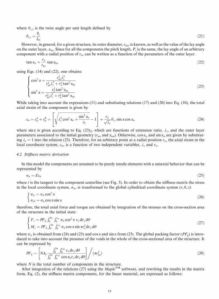
the stiffness matrix is a function of only the extension ratio of the structure, kz, global packing factor, PFg, andthe outer layer geometrical parameters of the structure in the initial state (reo and aeo). Since the stiffness ma-trix components depend on the strain, this model is essentially non-linear, but for the interval [1.001 1.04] ofextension ratio (practical strain range for aramid), kz, the results can be considered as constant. In the follow-ing, the results for the same axial strain (kz = 1.01) are presented.

5. Models comparison

The previous models have been applied to a strand of a 205 ton aramid cable of known constructionparameters (given by the cable supplier) shown in Table 1.

Table 1Available construction parameters for strand of 205 T aramid cable

Outer diameter 18.3 (mm)Pitch length 275 (mm)Components number 42Component axial stiffness, kc

a 346.1 kN

a kc obtained from experiments.

Table 2Necessary input data for all models

Models Input data

Raoof and Hoppe Pitch length, number of layers, components number per layer, component radius, Young’s modulus of component

Leech Pitch length, number of layers, component number per layer, components radius, component axial stiffness, kc, PFfor each layer

Continuum Strand radius, Pitch length, Young’s modulus of component, PFg

12

Table 2 shows the input data necessary for all models.Comparing Tables 1 and 2 shows that input data are missing for all the models. A sensitivity analysis has

been performed elsewhere by Ghoreishi (2005), and the results have shown that the overall behavior is notsensitive to these missing values for the practical structures of interest here (aeo 6 15�). Some illustrative partsof this sensitivity analysis are reported hereafter.

As it has been previously mentioned, it is practically difficult to represent the strand cross-section with amultilayered structure. Therefore, several multilayered discretizations can be a priori defined. From the valueof the strand radius and assembled yarn surface, it has been considered that the strand was made with fourlayers. The results obtained with the Leech’s model corresponding to three different multilayered discretiza-tions are given in Table 3, with very small differences.

The influence of the packing factor has also been studied, since this parameter is not defined at the localscale (i.e. in each layer) when the Leech’s model is used. A four layers discretization with respectively 1, 6,14 and 21 assembled yarns in each layer, has been considered, with three different values of the radius ofthe assembled yarn. For a given value of this radius, the packing factor of the layers 2–4 was constant andcalibrated in order to obtain a cross-section radius consistent with the strand radius value. The results arelisted in Table 4, where it can be checked that they are slightly sensitive to the packing factor values.

Therefore, for the present study, the values for the missing data were taken as follows:Number of layers is chosen to be 4.Component numbers for each layer are 1, 6, 14 and 21 and the PF in each layer are 1, 0.75, 0.88 and 0.89

respectively.On the other hand, Eq. (28) gives a global packing factor, PFg = 0.86. This value is in agreement with the

previous values used in the Leech’s model, which shows that both models have the same quantity of materialin the cross-section of the structure.

Table 3Results obtained for Leech’s model for different multilayer discretizations of the strand made of 42 assembled yarns distributed in fourlayers

Multilayered discretization kee (103 kN) keh (kN m) khe (kN m) khh (N m2)

1 + 6 + 14 + 21 14.1 13.3 13.0 21.71 + 7 + 14 + 20 14.1 13.1 12.8 21.43 + 8 + 13 + 18 14.1 13.0 12.7 21.5

Table 4Results obtained for Leech’s model for different values of Packing factor

Assembled yarn radius (mm) PF of layers 2–4 kee (103 kN) keh (kN m) khe (kN m) khh (N m2)

1.31 0.866 14.1 13.3 13.0 21.71.35 0.921 14.1 12.9 12.7 21.11.38 0.958 14.1 12.9 12.7 21.0

Table 5Results obtained for different models applied to the strand of 205 T aramid cable

Models kee (103 kN) keh (kN m) khe (kN m) khh (N m2) keh�khekehð%Þ

Raoof Full slip 14.1 13.5 13.7 19.0 1.48No-slip 14.7 7.72 9.27 105 20

Hoppe 14.1 – – – –Leech l = 0 14.1 13.3 13.0 21.7 2.26

l = 0.15 14.1 13.3 13.5 22.1 1.50l = 0.3 14.2 13.4 13.9 22.9 3.73

Continuum model 14.1 13.2 13.1 16.5 0.76

13

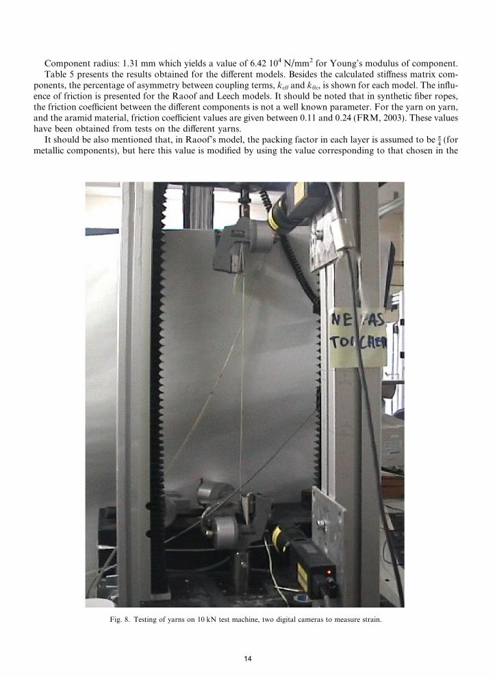
Component radius: 1.31 mm which yields a value of 6.42 104 N/mm2 for Young’s modulus of component.Table 5 presents the results obtained for the different models. Besides the calculated stiffness matrix com-

ponents, the percentage of asymmetry between coupling terms, keh and khe, is shown for each model. The influ-ence of friction is presented for the Raoof and Leech models. It should be noted that in synthetic fiber ropes,the friction coefficient between the different components is not a well known parameter. For the yarn on yarn,and the aramid material, friction coefficient values are given between 0.11 and 0.24 (FRM, 2003). These valueshave been obtained from tests on the different yarns.

It should be also mentioned that, in Raoof’s model, the packing factor in each layer is assumed to be p4

(formetallic components), but here this value is modified by using the value corresponding to that chosen in the

Fig. 8. Testing of yarns on 10 kN test machine, two digital cameras to measure strain.

14

FRM software, as well as the global packing factor for the continuum model. Indeed, the same structure isdefined for all the models (same material quantity in the structure).

The main conclusion from Table 5 is that all the models yield very similar results for the axial stiffness, kee.The difference for the coupling terms is visible. Only the torsion term results, khh, are significantly different forthe different models.

To show which model gives more reliable results (particularly for the torsion term, khh), it would be nec-essary to be able to compare them to experimental results.

In Raoof’s model, the structure in the no-slip case is much stiffer than in full-slip, however the couplingterms are smaller in the no-slip case. On the other hand, except for the axial stiffness where the two limit caseresults are similar, the differences between the two cases are significant, particularly for the torsion term. It isinteresting to note that the orthotropic sheet theory presented for the multilayered metallic cables by Raoof,and based on the contact theory between the metallic components with circular cross-section, yields resultscompletely comparable with those obtained from other specific models for synthetic cables.

The model of Hoppe provides a similar value for the axial stiffness but does not allow the other stiffnessterms to be obtained.

The results from Leech’s model show that the friction effect can be neglected for axial loading. However, itshould be mentioned that while the friction effect plays a small role in global stiffness behavior of such struc-tures, the effect of friction on the long-term performance and durability of a structure under cyclic loading canbe significant.

Then, the theoretical predictions will be compared to experimental results which are obtained from tractiontest on two different structures.

6. Experimental results

Experimental studies have been performed at two scale levels, first on yarns to determine the base compo-nent properties and then on two different assembled yarns which represent the multilayer structure.

Tensile tests at the yarn level give an indication of the material behavior without the effects of twist andconstruction. They were performed on a 10 kN test machine at an applied crosshead displacement rate of50 mm/min. Elongation was measured using two digital cameras, which record the movements of marks onthe yarns, as shown in Fig. 8. The test procedure for these and all subsequent tests was to apply five bed-ding-in load–unload cycles up to 50% of the nominal break load, before the load cycle which was used forthe modeling. This is standard practice in rope testing and stabilizes the material and construction.

An example of the yarn test results including the five bedding-in cycles and the test to failure is shown inFig. 9.

0

100

200

300

400

500

600

0 0.5 1 1.5 2 2.5 3

Forc

e (N

)

Strain (%)

Fig. 9. Force–strain plot for tensile test on 336 tex aramid yarn (Twaron 1000), five cycles to 50% of break load followed by test to failure.

15

Chailleux and Davies (2003) have also used yarn tests to identify the intrinsic viscoelastic and viscoplasticbehaviour of the aramid fibers used in the present study (Twaron 1000).

In order to provide data for correlation with the models, tests were then performed on two different assem-bled yarns taken from a 25 ton break load rope, Fig. 10 (at least five specimens were characterized for each),for which the construction parameters are given in Table 6. All the samples were made with the same aramidfiber grade. The load was introduced through cone and spike end connections. Tests involved applying fiveinitial bedding-in cycles, as for the yarn tests, by loading the samples to 50% of their nominal break loadat a loading and rate of 50 mm/min then unloading at the same rate. The same image analysis system wasused, measuring the displacements of two marks bonded to the assembled yarn (Fig. 10). From the tests

Fig. 10. Test on assembled yarn sample on 200 kN test machine, showing sample and two digital cameras to measure strain.

16

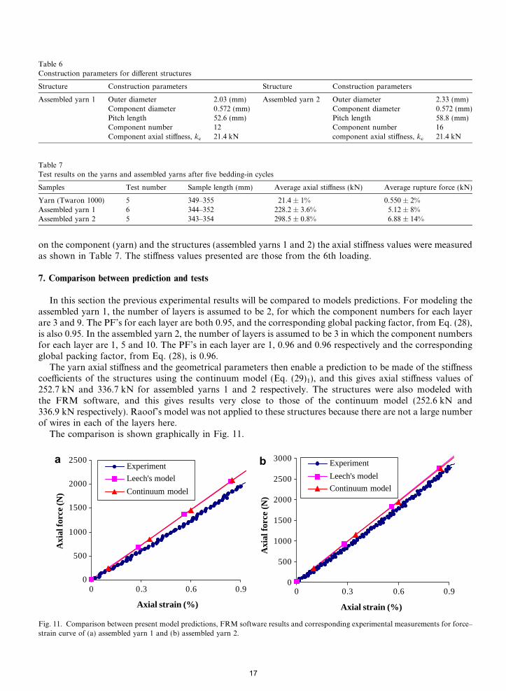
on the component (yarn) and the structures (assembled yarns 1 and 2) the axial stiffness values were measuredas shown in Table 7. The stiffness values presented are those from the 6th loading.

7. Comparison between prediction and tests

In this section the previous experimental results will be compared to models predictions. For modeling theassembled yarn 1, the number of layers is assumed to be 2, for which the component numbers for each layerare 3 and 9. The PF’s for each layer are both 0.95, and the corresponding global packing factor, from Eq. (28),is also 0.95. In the assembled yarn 2, the number of layers is assumed to be 3 in which the component numbersfor each layer are 1, 5 and 10. The PF’s in each layer are 1, 0.96 and 0.96 respectively and the correspondingglobal packing factor, from Eq. (28), is 0.96.

The yarn axial stiffness and the geometrical parameters then enable a prediction to be made of the stiffnesscoefficients of the structures using the continuum model (Eq. (29)1), and this gives axial stiffness values of252.7 kN and 336.7 kN for assembled yarns 1 and 2 respectively. The structures were also modeled withthe FRM software, and this gives results very close to those of the continuum model (252.6 kN and336.9 kN respectively). Raoof’s model was not applied to these structures because there are not a large numberof wires in each of the layers here.

The comparison is shown graphically in Fig. 11.

Table 6Construction parameters for different structures

Structure Construction parameters Structure Construction parameters

Assembled yarn 1 Outer diameter 2.03 (mm) Assembled yarn 2 Outer diameter 2.33 (mm)Component diameter 0.572 (mm) Component diameter 0.572 (mm)Pitch length 52.6 (mm) Pitch length 58.8 (mm)Component number 12 Component number 16Component axial stiffness, kc 21.4 kN component axial stiffness, kc 21.4 kN

Table 7Test results on the yarns and assembled yarns after five bedding-in cycles

Samples Test number Sample length (mm) Average axial stiffness (kN) Average rupture force (kN)

Yarn (Twaron 1000) 5 349–355 21.4 ± 1% 0.550 ± 2%Assembled yarn 1 6 344–352 228.2 ± 3.6% 5.12 ± 8%Assembled yarn 2 5 343–354 298.5 ± 0.8% 6.88 ± 14%

0

500

1000

1500

2000

2500

0 0.3 0.6 0.9

Axial strain (%)

Axi

al fo

rce

(N)

Experiment

Leech's model

Continuum model

0

500

1000

1500

2000

2500

3000

0 0.3 0.6 0.9

Axial strain (%)

Axi

al f

orce

(N

)

Experiment

Leech's model

Continuum model

a b

Fig. 11. Comparison between present model predictions, FRM software results and corresponding experimental measurements for force–strain curve of (a) assembled yarn 1 and (b) assembled yarn 2.

17

So far all the tests performed have concentrated on the axial stiffness kee by testing structures with fixed endloading conditions. However, a small number of tests have shown that there is not measurable tension–torsioncoupling terms and torsion stiffness for the small diameter assembled yarns at this level. In order to determinethe other coefficients (coupling terms and torsion term) and to compare them with predicted values test resultsfor the higher level such as strands of 205 T fiber rope would be necessary.

8. Conclusion

A non-linear elastic continuum model has been developed for the analysis of the overall axial stiffness offibrous structures with a large number of twisted components. By contrast with multilayered approaches,the structure under consideration is herein depicted as a set of coaxial helixes only characterized by their exter-nal lay angle and corresponding radius. The constitutive material is assumed to be linear. Static monotonicaxial loads are considered, the inter-fiber friction effects are not taken into account. Moreover, the studiedstructures exhibiting small lay angles, the overall diametral contractions are neglected, which may contributeto the overestimation of stiffness. The analytical model developed leads to useful closed-form expressions thusallowing rope constructions to be optimized.

Due to lack of published experimental data, the model has first been compared with models of the litera-ture. The results obtained, have shown that all the models give results that agree reasonably well with eachother, except with respect to the torsion stiffness, for which there is a significant difference. In addition, stiff-ness matrices of all the models deviate slightly from symmetry and this lack of symmetry is due to a certainlack of consistency in the various simplifying hypotheses.

Tensile tests have then been performed on aramid fiber assemblies with two structures, to obtain the axialstiffness. The preliminary test results indicate a good correlation with the model. Additional test data, espe-cially to examine tension–torsion and pure torsion loading, are needed to gauge performance of the models.The integration of these results in a model for a large aramid wire rope and comparison with tension and ten-sion–torsion coupling test results will be described in Part II (Ghoreishi et al., in press) of this paper.

References

Beltran, J.F., Rungamornrat, J., Williamson, E.B., 2003. Computational model for the analysis of damage ropes. In: Proceedings of Thethirteenth International Offshore and Polar Engineering Conference, Honolulu, Hawai, USA.

Beltran, J.F., Williamson, E.B., 2004. Investigation of the damage-dependent response of mooring ropes. In: Proceedings of TheFourteenth International Offshore and Polar Engineering Conference Toulon, France.

Blouin, F., Cardou, A., 1989. A study of helically reinforced cylinders under axially symmetric loads mathematical modelling.International Journal of Solids and Structures. 25 (2), 189–200.

Chailleux, E., Davies, P., 2003. Modelling the non-linear viscoelastic and viscoplastic behaviour of aramid fiber yarns. Mechanics of TimeDependent Materials Journal 7 (3–4), 291–303.

Crossley, J.A., Spencer, A.J.M., England, A.H., 2003a. Analytical solutions for bending and flexure of helically reinforced cylinders.International Journal of Solids and Structures 40 (4), 777–806.

Crossley, J.A., England, A.H., Spencer, A.J.M., 2003b. Bending and flexure of cylindrically monoclinic elastic cylinders. InternationalJournal of Solids and Structures 40 (25), 6999–7013.

Foster, G.P., 2002. Advantages of fiber rope over wire rope. Journal of Industrial Textiles 32 (1), 67–75.FRM, Fibre Rope Modeller, version 1.1.5, 2003. Software development for Tension Technology International Ltd. (TTI).Ghoreishi, S.R., 2005. Modelisation analytique et caracterisation experimentale du comportement de cables synthetiques. Ph.D. Thesis,

Ecole Centrale de Nantes, France.Ghoreishi, S.R., Davies, P., Cartraud, P., Messager, T., in press. Analytical modeling of synthetic fiber ropes, part II: A linear elastic

model for 1 + 6 fibrous structures. International Journal of Solids and Structures, doi:10.1016/j.ijsolstr.2006.08.032.Hobbs, R.E., Raoof, M., 1982. Interwire slippage and fatigue prediction in stranded cables for TLP tethersBehaviour of Offshore

Structures, 2. Hemisphere publishing/McGraw-Hill, New York, pp. 77–99.Hoppe, L.F.E., 1991. Modeling the Static Behavior of Dyneema in Wire-rope Construction. MTS RTM.Jolicoeur, C., Cardou, A., 1994. An analytical solution for bending of coaxial orthotropic cylinders. Journal of Engineering Mechanics 120

(12), 2556–2574.Jolicoeur, C., Cardou, A., 1996. Semicontinuous mathematical model for bending of multilayered wire strands. Journal of engineering

Mechanics 122 (7), 643–650.Leech, C.M., 2002. The modeling of friction in polymer fibre rope. International Journal of Mechanical Sciences. 44, 621–643.

18

Leech, C.M., Hearle, J.W.S., Overington, M.S., Banfield, S.J., 1993. Modelling tension and torque properties of fibre ropes and splices. In:Proceeding of the Third International Offshore and Polar Engineering Conference Singapore.

Mindlin, R.D., 1949. Compliance of elastic bodies in contact. Journal of Applied Mechanics 16, 259–268.Raoof, M., 1983. Interwire contact forces and the static, hysteretic and fatigue properties of multi-layer structural strands. Ph.D. Thesis,

Imperial College of Science and Technology, London, UK.Raoof, M., 1991. Method for analysing large spiral strands. Journal of Strain Analysis 26 (3), 165–174.Raoof, M., Hobbs, R.E., 1988. Analysis of multilayered structural strands. Journal of engineering Mechanics 114 (7), 1166–1182.Raoof, M., Kraincanic, I., 1995a. Simple derivation of the stiffness matrix for axial/torsional coupling of spiral strands. Computers and

Structures 55 (4), 589–600.Raoof, M., Kraincanic, I., 1995b. Analysis of large diameter steel ropes. Journal of Engineering Mechanics 121 (6), 667–675.Rungamornrat, J., Beltran, J.F., Williamson, E.B., 2002. Computational model for synthetic-fiber rope response. In: Proceeding of

Fifteenth Engineering Mechanics Conference. ASCE, New York.

19