ANALYTICAL METHODS APPLIED TO THE MEASUREMENTS OF DEFLECTIONS AND WAVE VELOCITIES ON HIGHWAY PAVEMENTS: PART 1,

MEASUREMENTS OF DEFLECTIONS

By

W. H. Cogill Research Associate

Research Report 32-14

Extension of . AASHO Road Test Results

Research Project Number 2-8-62-32

Sponsored By

The Texas Highway Department In Cooperation with the

U. S. Department of Transportation Federal Highway Administration

Bureau of Public Roads

March, 1969

TEXAS TRANSPORTATION INSTITUTE Texas A&M University

College Station, Texas

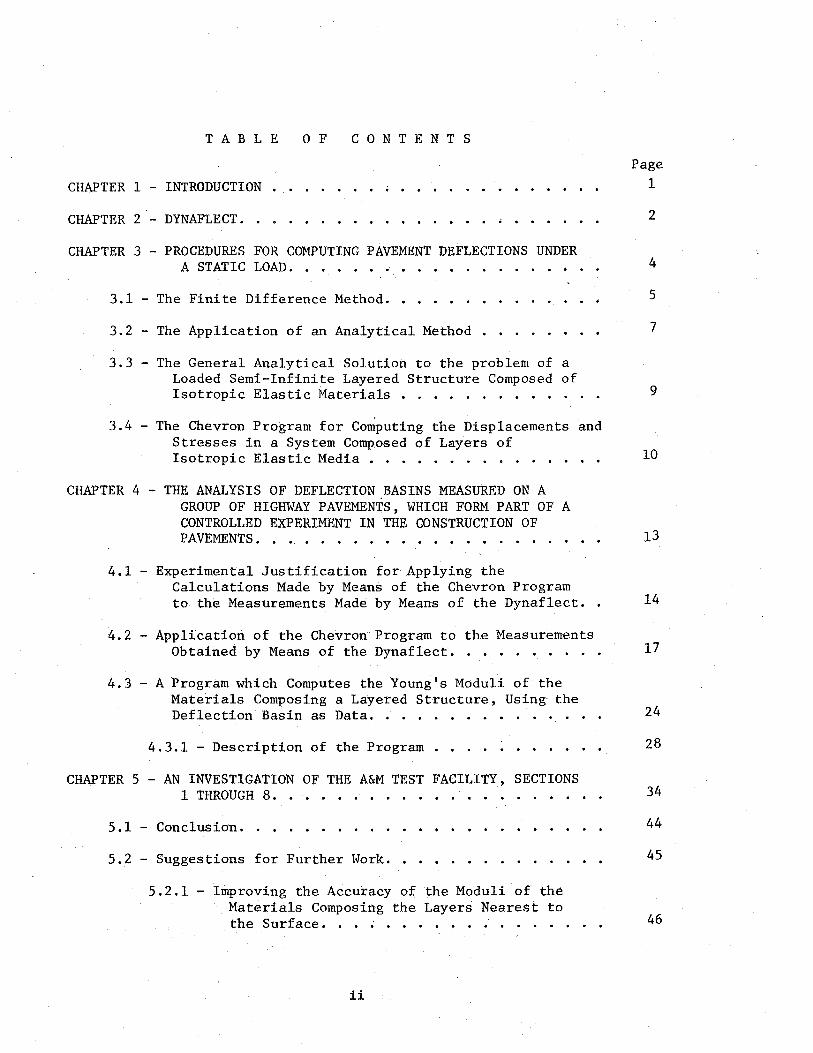
TABLE 0 F C 0 N T E N T S

CHAPTER 1 - INTRODUCTION

CHAPTER 2 - DYNAFLECT.

CHAPTER 3 - PROCEDURES FOR COMPUTING PAVEMENT DEFLECTIONS UNDER A STATIC LOAD ..••...•

3.1 - The Finite Difference Method ..

3.2 - The Application of an Analytical Method

3.3- The General Analytical Solution to the problem of a Loaded Semi-Infinite Layered Structure Composed of Isotropic Elastic Materials • • . . . . . . .

3.4 - The Chevron Program for Computing the Displacements and Stresses in a System Composed of Layers of Isotropic Elastic Media . • . . . • . . .

CHAPTER 4 - THE ANALYSIS OF DEFLECTION BASINS MEASURED ON A GROUP OF HIGHWAY PAVEMENTS, WHICH FORM PART OF A CONTROLLED EXPERIMENT IN THE CONSTRUCTION OF PAVEMENTS. . . • . • . • • . • • • • • . . .

4.1 - Experimental Justification for Applying the Calculations Made by Means of the Chevron Program to the Measurements Made by Means of the Dynaflect ..

4.2 - Application of the Chevron Program to the Measurements Obtained by Means of the Dynaflect. . ••.

4.3 -A Program which Computes the Young's Moduli of the Materials Composing a Layered Structure, Using the Deflection Basin as Data. . • •

4.3.1 - Description of the Program

CHAPTER 5- AN INVESTIGATION OF THE A&M TEST FACILITY, SECTIONS 1 THROUGH 8. . . . . . . . . . .

5.1 - Conclusion.

5.2 - Suggestions for Further Work.

5.2.1 - Improving the Accuracy of the Moduli of the . Materials Composing the Layers Nearest to

the Surface. . . . . • . . . • _. • . . . .

ii

Page 1

2

4

5

7

9

10

13

14

17

24

28

34

44

45

46

5.2.2 - Extension of the Work in Order That the Loading Conditions May Correspond With Those Imposed

Page

By Traffic. . . • . . • . . . 4 7

APPENDIX A - THE OPERATION OF THE CHEVRON PROGRAM 48

A.l - The Accuracy of the Chevron Program. . 49

A.l.l - The Accuracy of Representing the Applied Load 50

A.l.2 - The Accuracy of Representing the Vertical Settlements at the Free Surface • 52

APPENDIX B - FAULT TRACING IN THE CONVERGENCE PROGRAM 54

B.l - First Operational Suggestion •

B.2 - Second Operational Suggestion.

APPENDIX C - A NOTE ON THE SOLUTIONS OF THE EQUATIONS REPRESENTED BY THE "C" AND "D" MATRICES.

APPENDIX D - COMPARISON BETWEEN THE DEFLECTIONS CAUSED IN A · STRUCTURE REPRESENTING A HIGHWAY PAVEMENT BY A

TRUCK WHEEL WITH THOSE CAUSED BY THE DYNAFLECT AND

56

56

58

BY A 12 II PLATE . • . • . . . • . . . • . 59

APPENDIX E - LIST AND DESCRIPTIONS OF THE COMPUTER PROGRAMS ASSOCIATED WITH PART 1 OF THIS REPORT.

APPENDIX F - THE PLOTTING OF THE CROSS SECTION OF THE DEFLECTIONS BASIN IN A PAVEMENT WHICH IS SUBJECTED TO A

63

POINT LOAD • . • • . . • . • . . . . . • . • . . • 65

iii

LIST OF FIGURES

Figure Page

1 Results of Pavement Deflection Measurements Obtained by Means of

2

3

4

5

6

7

8

9

the Dynaflect. Operation over a Range of Frequencies. 15

Observed Pavement Deflections (circled points) Compared With Calculations Made by Means of the Chevron Program, Using the Values shown for the Young's Moduli of the Materials Used in the Construction . . • . . • . • .

Values of the Estimated E's P:Lot~ed Against the "b's" Determined by Scrivner and Moore . . . . . • . . . .

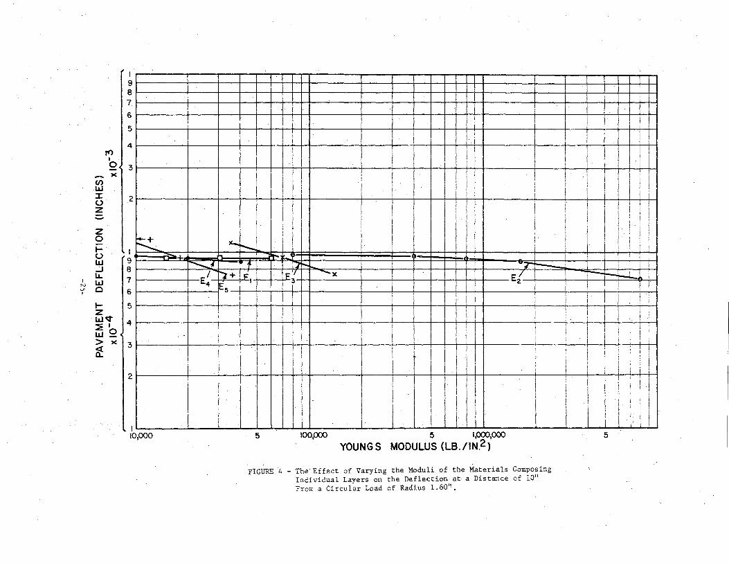
The Effect of Varying the Moduli. of the Materials Composing Individual Layers on the Deflection at a Distance of 10" From a Circular Load of Radius 1. 60" . . . . . . . . . .

Block Diagram of the Computer Program Used to Interpolate by Iteration the values of the Young's Moduli for the Individual Layers in order that the Calculated Deflections May Correspond with the Measured Deflection Basin •••..

Values of Young's Modulus for the Materials Composing the Layers of the Structures, Sections 1 Through 8 ..

The Correspondence Between A Specified Vertical Load and the Vertical Direct Stresses Calculated by the Chevron Program in the Vicinity of the Load .....

The Effect of Changes in the Young's Moduli of the Materials Composing a Two-Medium Structure on the Deflections Measured by Means of (1) a Truck Wheel (2) a Dynaflect (3) a 12-Inch Plate ••.•.••.....•..•

Hypothetical Plot of the Results of the Measurements of the Deflections on the Surrace of a Pavement Subjected to a

· Point Load . . . . . . . . . . . . . . . . . . . . . . . .

.. iv

18

23

25

29

39

51

60

66

LIST OF TABLES

Table

1 Table of Values of E Selected for the Initial Computations Required for Section 3 of the A&M Test Facility • •

2 Data Cards for Input to the Convergence Prograrit wHC36 and

26

the Data Checking Program WHC35 • • • • • • • • ~ • • 31

3 Typical Output from the Data Checking Program WHC35 33

4 Typical Output from the Convergence Program WHC36 • • • 35

5 Root Mean Square Residuals Used for Checking the Performance of the Convergence Program. Data from the A&M Test Facility, Sections 1 through 8. • • • • • • • • • • • • • • • • • • • 3 7

6 Values of Young's Modulus for the Materials Composing the Layers of the Structures, Sections 1 through 8 • • • • • • • • • • • • 38

7 The Effect of Halving the )'oung's Modulus of the Materials Composing each of the Layers on Pavement Deflection Measured at a Distance of 10" from the Load. Table 7 (a) .... Section 2, Table 7 (b) -Section 6 • . . . . . . . . • . . . . . . . . . . . . . . . . . 41

8 A Comparison Between the Vertical Settlements at the Surface of a Layered Structure Calculated by Means of the Chevron Program, and the True Settlements for a Similar System • • • • • • • • • 53

v

ACKNOWLEDGEMENTS

The research reported herein was done by the Texas Transportation

Institute, Texas A&M University in cooperation with the Texas Highway

Department, and was sponsored jointly by the Texas Highway Department

and the Department of Transportation, Federal Highway Administration,

Bureau of Public Roads.

The opinions, findings, and conclusions expressed in this publica­

tion are those of the author and not necessarily those of the Bureau of

Public Roads.

vi

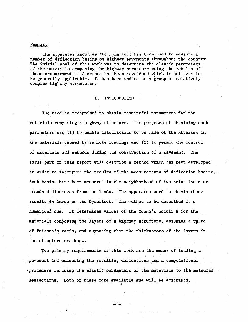
Sunnnary

The apparatus known as the Dynaflect has been used to measure a number of deflection basins on highway pavements throughout the country. The initial goal of this work was to determine the elastic parameters

· of the materials composing the highway structure using the results of these measurements. A method has been developed which is believed to be generally applicable. It has been tested on a group of relatively complex highway structures.

1. INTRODUCTION

The need is·recognized to obtain meaningful parameters for the

materials composing a highway structure. The purposes of obtaining such

parameters are (1) to enable calculations to be made of the stresses in

the materials caused by vehicle loadings and (2) to permit the control

of materials and methods during the construction of a pavement. The

first part of this report will describe a method which has been developed

in order to interpret the results of the measurements of deflection basins.

Such basins have been measured in the neighborhood of two point loads at

standard distances from the loads. The apparatus used to obtain these

results is known as the Dynaflect. · The method to be described is a

numerical one. It determines values of the Young's moduli E for the

materials composing the layers of a highway structure, assuming a value

of Poisson's ratio, and supposing that the thicknesses of the layers in

the structure are know.

Two primary requirements of this work are the means of loading a

pavement and measuring the resulting deflections and a computational

·procedure relating the elastic parameters of the materials to the measured

deflections. Both of these were available and will be described.

-1-

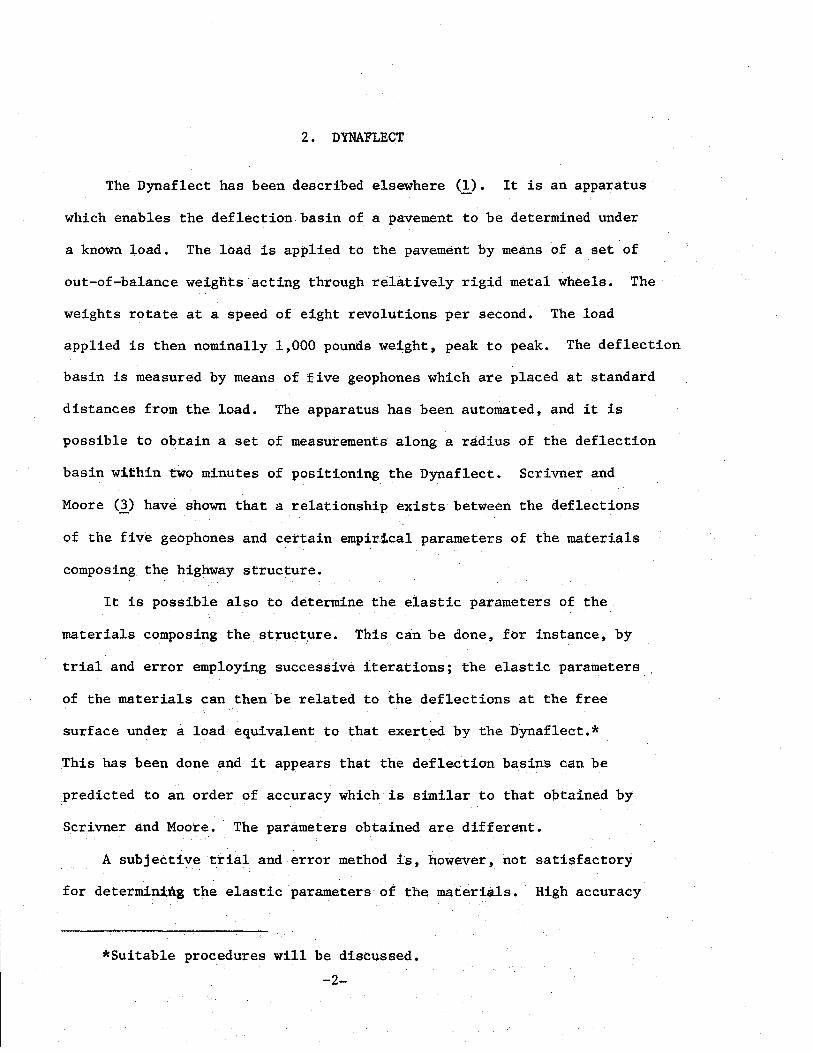
2. DYNAFLECT

The Dynaflect has been described elsewhere (1). It is an apparatus

which enables the deflection basin of a pavement to be determined under

a known load. The load is applied to the pavement by means of a set of

out-of-balance weignts·acting through relatively rigid metal wheels. The

weights rotate at a speed of eight revolutions per second. The load

applied is then nominally 1,000 pounds weight, peak to peak. The deflection

basin is measured by means of five geophones which are placed at standard

distances from the load. The apparatus has been automated, and it is

possible to obtain a set of measurements along a radius of the deflection

basin within two minutes of positioning the Dynaflect. Scrivner and

Moore (~) have shown that a relationship exists between the deflections

of the five geophones and certain empiri.cal parameters of the materials

composing the highway structure.

It is possible also to determine the eiastic parameters of the

materials composing the structure. This can be done, for instance, by

trial and error employing successive iterations; the elastic parameters

of the materials can then be related to the deflections at the free

surface under a load equivalent to that exerted by the D)rnaflect.*

This has been done and it appears that the deflection basins can be

predicted to an order of accuracy which is similar to that obtained by

Scrivner and Moore. The parameters obtained are different.

A subjective trial and error method is, however, not satisfactory

for determin:b\g the elastic parameters of the materials. High accuracy

*Suitable procedures will be discussed.

-2-

cannot be achieved. An objective method is needed in order to determine

values of the elastic parameters which yield a deflection basin closely

approximating the measured one.

-3-

3. PRO.CEDURES FOR COMPUTING PAVEMENT DEFLECTIONS UNDER A STATIC LOAD

There is no direct method for calculating the elastic parameters of

a layered structure such as a highway pavement. However, there are two

distinct methods available for calculating the surface displacements when

the parameters of the materials composing the structure are given. These

methods will be discussed in the sections which follow. The first, a

finite difference method, enables the required quantities to be determined

at discrete mesh points within the system, but readily incorporates non­

linear stress-strain behavior. The second, an analytical method, provides

a solution which is defined at all points in the coordinate system, although

the associated definition of the applied load is arduous. The method of

solution and the handling of data vary ... The choice of method is governed

by the input data available and the results which are required.

-4-

3.1 The Finite Difference Method

The differential equations of elasticity, which are assumed to govern

the displacements within a highway structure, are solved by considering

the particle displacements at the modal points of a mesh (!). For this

purpose the differential equations are expressed not in terms of continuous

space coordinates (x, y, z), but in terms of the spacing between the mesh

points. The particle displacements (u, v, w) in the direction of the

axes are, therefore, regarded as varying·not continuously but in discrete

steps when passing from one mesh point to the next. The difference between

the coordinates of neighboring mesh points is finite, not infinitesimal

as in the solution by analytical methods.

The problem becomes the solution of a large number of simultaneous.

equations (three for each mesh point), in order that the differential

equations of elasticity may be satisfied.

As the mesh points are made successively closer, the finite difference

solution approaches the solution obtained by analytical means. The finite

difference method can be used in cases where the elastic parameters vary in

an arbitrary way; variation from one nodal point to the next can be specified

as part of the problem data. This can be done with no essential complication

to the computing program. Non-linearity in a stress-strain response can be

similarly handled, or the stress-strain relationship can be defined in a

subroutine to save the labor of data punching.

The spacing between the mesh points can be varied to provide a greater

density of information in significant regions. In the transition from a

region of coarse to one of fine spacing, however, the displacements at

-5-

points at the zone interface need careful consideration; these represent

the boundary conditions of a zone of relatively fine mesh, and the accuracy

requirements may differ from those within a coarse mesh.

-6-

3.2 The Application of an Analytical Method

The deflections on the surface of a semi-infinite isotropic elastic

solid may be determined by analytical means. If the solid is uniform,

closed analytical solutions are available for certain simple loading

systems. The case of a point load applied at the free surface has been

discussed by Timoshenko (~). The result is obtained by using a trial

solution of the equations of elasticity, which involves two arbitrary

constants. One of these is eliminated by means of the physical condition

that the shearing stress in a vertical plane at the free surface must be

zero. In order to determine the second in terms of the applied load,

elementary annuli of wedge-shaped cross section are considered; these

annuli form a hemisphere centereD on the point at the surface at which

the load is applied. The net vertical forces acting on these annuli

are summed and equated to the applied load, thus fixing the second of

the constants. The deflection at the free surface is inversely proportional

to the distance from the point at the surface at which the load acts.

By means of a formal solution of the equations of elastic equilibrium,

Love (~) obtained expressions for the displacements at any point on or

within such a medium; the force is considered to be applied to a point on

the free surface. The deflection at the free surface is inversely pro­

portional to the distance from the line of action of the load.

Perhaps the clearest solution to the problem is given by Filenko­

Borodich (l). As in the solution given by Timoshenko, a hemisphere is

-7-

considered which is centered on the load point at the free surface. The

sum of the vertical forces acting on the elements of this surface are

equated to the applied load. Only one arbitrary constant is introduced

throughout. Its value is found, as indicated, in terms of the applied

load. The vertical deflection at the .free surface is, as before, inversely

proportional to the distance frotn the point at which the load is applied.

This solution for the elementary case of a::continuous~homogeneous

semi-infinite isotropic elastic solid suggests a method of plotting the

results (§). If the logarithm of the deflection is plotted against the

logarithm of the spacing (the distance between the applied load and the

point at which deflection is measured on the free surface), the graph

will have a slope of 45°; If however (deflection x spacing) is plotted

against spacing on double logarithmic paper, the gr-aph will have a

constant ordinate for the (deflection x spacing).product. This provides

a useful basis for judging the departure from homogeneity of any real

structure.

-8-

3. 3 The General Analytical Solution to the Problem of a Loaded Semi-Infinite Layered Structure Composed of Isotropic Elastic Materials

Using the equations of elasticity in cylindrical coordinates,

Burmister (~) obtained expressions for the stresses and displacements

in a structure composed of layers of materials having dissimilar elastic

parameters. The vertical stress at the free surface is assumed to be a

Bessel function of the radial spacing. This choice of stress as a boundary

condition makes it possible to satisfy the differential equations of

elasticity using relatively simple stress functions. Particular ap-

plications of the resulting solutions to two- and three-layer structures

are considered. Any form of surface loading can be represented by adding

a series of Bessel functions, such as Burmister assumed as a basic surface

stress. The loading can be synthesised analytically by means of a Fourier-

Bessel transform (10). Alternatively, it can be represented by a sum of

a number of Bessel functions, each with a different weighting coefficient.

-9-

3.4 The Chevron Program for Computing the Displacements and Stresses in a System Composed of Layers of Isotropic Elastic Media

The Chevron program (11, 12) for the computation of stresses and

displacements in a layered medium such as a highway structure has been

written using Burmister's theory as the starting point. The authors of

the program have extended Burmister's wor~ to permit the analysis of a

structure consisting of any number of layers supported by a foundation

which is of infinite depth and infinite lateral extent. The radially

synunetric differential equation of elastic equilibrium in cylindrical

coordinates (r, z), namely

is satisfied by a potential function <jl.(r, z, m) of the form l.

where m is a parameter, as it is in Burmister's papers (~),and i denotes

the ith medium in the layered structure.

The stresses and displacements in the system can then be expressed in

terms of the potential function <!r(r,z,m) by means of standard expressions

of elasticity (.2_, £, ]) . Beyond this point the approach adopted by the

authors of the Chevron program differs from that of Burmister. The stresses

and displacements, in terms of the arbitrary constants A., B., C1. and D.

l. l. l.

are written in matrix form in order to make the algebra more easy to grasp;

there is one set of constants Ai' Bi, Ci and Di for each layer denoted by

the subscript "i". The matrix expressions for the stresses and displHcements

at the bottom of layer "i" are

-10-

equated to those for the top of layer (i + 1}, This process can be continued

until the underlying semi-infinite medium is reached when i = n. The matrix

expression for the stresses and displacements in the nth medium has only

two arbitrary constants; the remaining two must be zero because both stresses

and displacements vanish at infinite depth. All of the A. 1 s, B. Is' C. IS and 1. ]_ 1.

D. 1 s may then be written in terms of the two arbitrary constants associated 1.

with the semi-infinite medium C and D . A and B are zero for the reason n n' n n

just given. In particular, the A1 , B1 , c1 and D1

can be written in terms

of C and D n n

(Because of the complexity of the expression, we should not

like--indeed we should not attempt--to write down the expressions for A1 ,

B1 , c1 and D1

in full: fortunately the computer does it for us, in carrying

out the successive matrix operations.) We are able to say something about

the arbitrary constants associated with the first layer, remembering that

they are now expressed in terms of only two unknown quantities, C and D . n n

They are related to the shear stress at the free surface in the (r,z) plane.

This shear stress must everywhere be zero, because of the way in which the

system is loaded. Second, the vertical stress at the free surface is defined

at all points on the surface. It is equal to a Bessel function of the radius,

multiplied by a weighting function, p(m). Using these two additional

boundary conditions the problem is so;lved.

It is possible to repeat this calculation using a series of values of

m; the vertical surface stresses are then superposed in proportion to their

weighting functions p(m). Using a method similar to that employed to determine

a Fourier series, it is possible to determine a spectrum of weighting functions

p(m) which will represent any desired surface loading (10). This is done in

-11-

a subsequent stage of the Chevron program. The surface load which is

represented is a circular area on which the vertical pressure is every­

where the same, and the surface shear stresses are zero. The load thus

corresponds with that exerted by a flexible plate which is able to follow

the deformed shape of the surface of the structure being loaded.

When the weighting coefficients have been determined, the stresses

and displacements obtained for each value of "m" are superposed. This

yields the final result. See the Appendix for a description of the

operating method for the Chevron program.

-12-

4. THE ANALYSIS OF DEFLECTION BASINS MEASURED ON A GROUP OF HIGHWAY PAVEMENTS, WHICH FORM PART OF A

CONTROLLED EXPERIMENT IN THE CONSTRUCTION OF PAVEMENTS

There is a need to determine the elastic constants of the materials

used in constructing highway and airfield pavements. These depend on th~

state of compaction, as well as on the moisture content of the materials;

they are affected by ~hysical and chemical changes which occur during

the service life, such as comminution of the granular substances composing

the structure and the weathering action of the atmosphere. Laboratory

tests to determine the elastic parameters are, therefore, difficult to

apply in the field, as the exact field conditions and the history after

a period of use are so complex that they cannot be simulated.

Methods have been developed for the purpose of determining the elastic

' parameters of layered systems. Most of these depend, in principle, on the

measurement of a mechanical admittance (the measurement of a displacement

caused by a load). In the case of the Benkelman Beam, for example, the

load is effectively static (it is maintained at a fixed value for long

enough to allow any vibrations which it causes in the pavement to decay),

and the deflection is measured at a point in the neighborhood of the load.

The deflection basin caused by a static load can be measured by the same

or similar apparatus. This yields more information about the pavement

than a single point deflection.

-13-

4.1 Experimental justification for applying.the calculations made by means of the Chevron program to the measurements made by means of the Dynaflect ·

The calculations made by means of the Chevron program are based on

the assumption of isotropic, elastic substances under static load. The

effects of intertia and "viscous" damping do not need to be considered

as they do not affect the results. However, the Dynaflect applies a

load to the surface of the pavement which is not static but varies with

time. The variation is approximately sinusoidal, at a repetitive rate

of eight applications per second. The effects 'of inertia and material

damping are not necessarily negligihle, and some indication of their

effect is needed before applying calculations based on static conditions

to the Dynaflect measurements.

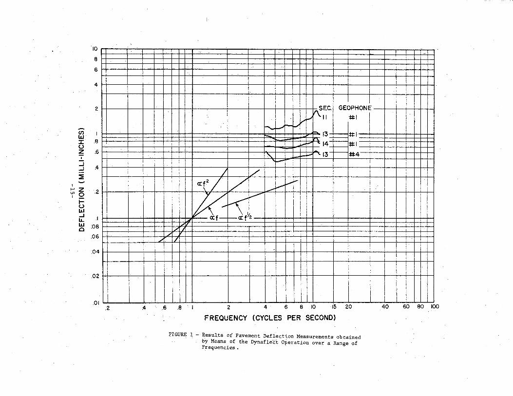
In order to estimate the effect of the applied load being other

than static, some experiments were carried out on a few highway structures

which have been constructed for experimental purposes. The surfaces of

selected sections were loaded by means of the Dynaflect and the deflection

basins measured according to the normal procedure used with the apparatus.

After modifications to the loading and measuring equipment, the same load

was applied at repetition rates varying from 4 c/s to 12 c/s. The deflection

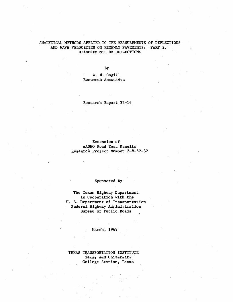
basins were measured at a number of frequencies of loading. The deflections

for a given spacing were plotted as a function of frequency of application

of the load. Typical results are shown in Figure 1. It appears that the

vertical deflections at the free surface are independent of the frequency

within the range of frequencies employed. The local increase of deflection

near 12 c/s is believed to be due to a mechanical resonance in the loading

-14-

C/) w ::r:: (.) z • ~ ~ -:?!

I 1-' z U1 0 I

1-(.) w ~ IJ... w 0

10

8

6

4

2

I

.8

.6

.2

I

:08

.06

.04

.0 2

.0 I

I I I

I I

I I

.2 4

I

I I I SEC., GEOPHONE

I I ~II :1:1:1

I - ....... ~~--' I -..... ~ 1-o.. 13-r---#I - t---

l,..ooo !""' '14-t--- #I ·- ,___ 13-r-+--' #4 I ··" -+-

' -I

/ /I

I oc(2/ L~ _l~ "" 1--'"

I v I i I

I I I i(_ :s;l !

I i ! I I I I A

/ !/

./i ~ Ll

I I .

I I ! I I

i

I

I I

I I .6 .8 2 4 6 8 10 15 20

FREQUENCY (CYCLES PER SECOND)

FIGURE 1 - Results of Pavement Deflection Measurements obtained by Means of the Dynafle-~i: Operation over a Range of Frequencies •

I

I I

l

I I I

1

'"

'

I I

I I

I I

I I I

I I

I

I

I

I I I

40 60 80 I 00

system of the Dynaflect. If effects of inertia were dominant, the deflections

should decrease with increasing frequency according to the square of the

frequency. The slope of the deflection-frequency curve should then be

downward and have a value of two decades vertical to one decade horizontal.

If a viscous type of damping were dominant, the curves would have a down­

ward slope of one decade vertical to one decade of horizontal change. No

such changes in deflections are observed, however. It is deduced that

both effects are unimportant within the range of frequencies investigated.

In particular, this is evidence that such effects are unimportant below

the upper limit of frequency investigated here; we shall, therefore, apply

the results of calculations, based on the assumption of static conditions,

to the measurements obtained by means of the Dynaflect.

In what follows, we shall investigate .. what is effectively the iteration

of the Chevron program, altering the Young's moduli of the materials composing

the layers until the calculated and measured deflection basins agree; the

f·inal values of the Young's moduli obtained are used as the moduli for

the materials. In order to save execution time, the actual Chevron program

was not iterated. Instead an approximation to the Chevron results was

established, which is simpler in form than the complete expressions for

deflections used in the Chevron program. This approximation, valid over

a limited range of values of the Young's moduli of the materials, was used

as the basis of an iterative solution for the moduli.

-16-

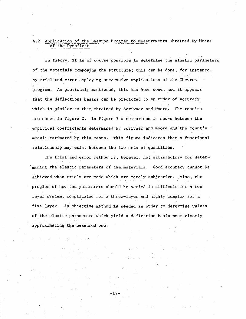
4.2 Application of the Chevron Program to Measurements Obtained by Means of the Dynaflect

In theory, it is of course possible to determine the elastic parameters

of the materials composing the structure; this can be done, for instance,

by trial and error employing succe~sive applications of the Chevron

program. As previously mentioned, this has been done, and it appears

that the deflections basins can be predicted to an order of accuracy

which is similar to that obtained by S.crivner and Moore. The results

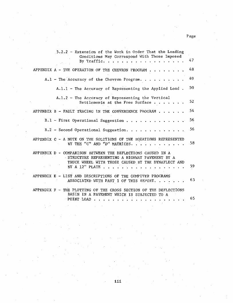
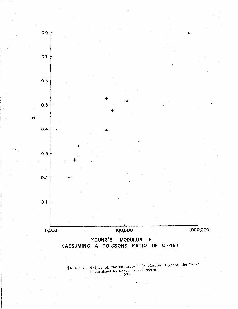
are shown in Figure 2. In Figure 3 a comparison is shown between the

empirical coefficients determined by Scrivner and Moore and the Young's

moduli estimated by this means. This figure indicates that a functional

relationship may exist between the two sets o:C quantities.

The trial and error method is, howev.er, not satisfactory for deter- .

mining the elastic parameters of the materials. Good accuracy cannot be

achieved when trials are made which are merely subjective. Also, the

proglem of how the parameters should be varied is difficult for a two

layer system, complicated for a three-layer and highly complex for a

five-layer. An objective method is needed in order to determine values

of the elastic parameters which yield a deflection basin most closely

approximating the measured one.

-17-

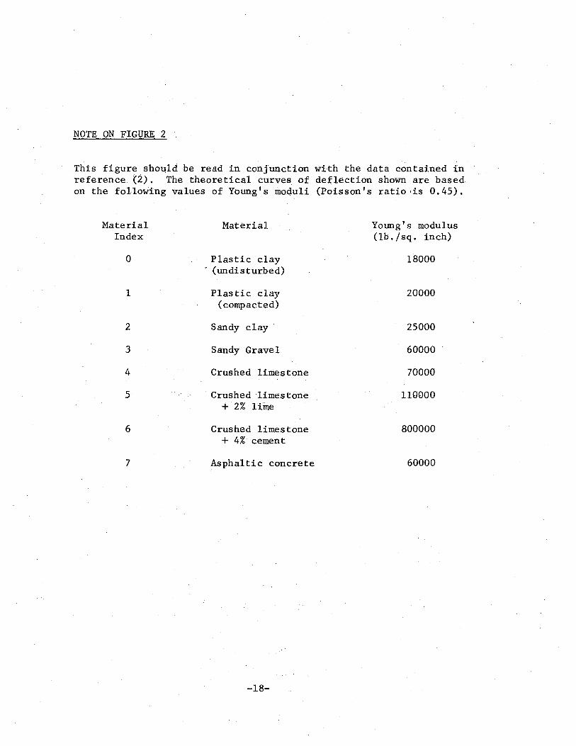
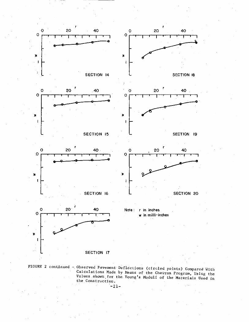
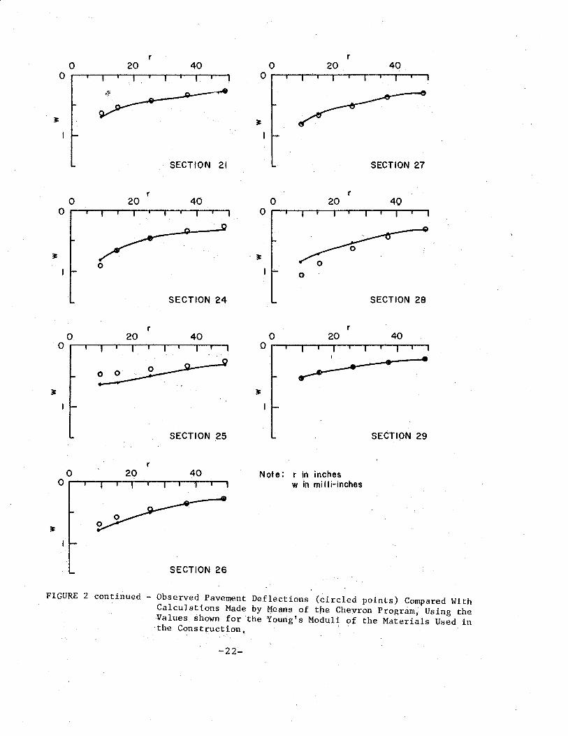
NOTE ON FIGURE 2

This figure should be read in conjunction with the data contained in reference (2). The theoretical curves of deflection shown are based on the following values of Young's moquli (Poisson's ratio ·is 0.45).

Material Index

0

1

2

3

4

5

6

7

Material

Plastic clay · (undisturbed)

Plastic clay (compacted)

Sandy clay

Sandy Gravel

Crushed limestone

Crushed limes tone + 2% lime

Crushed limestone + 4% cement

Asphaltic concrete

-18-

Young's modulus (lb. I sq. inch)

18000

20000

25000

60000

70000

110000

800000

60000

0 0

~I

2

0 0

~

o· 0

r r 20 40 0 20 40

0

0

0

0 ~I 0

0

0

0 SECTION I 2 SECTION 5

r 40

r 0 20 40

0

SECTION 2

r ~I 0

40 0

2 SECTION 6

Note : r in inches SECTION 3 w in miiiHnches

SECTION 4

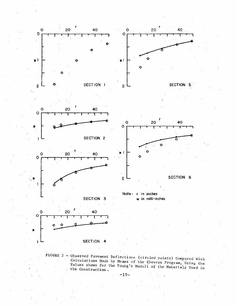
FIGURE 2 - Opserved Pavement Deflections (circled points) Compared With Calculations Made by Means of the Ghevron Program,Using the Values shown for the Young Is Moduli of the Materials Used in the Construction •

-19-

r r 0 20 40

0 r-~-r--~~-T~r--r~--~~

SECTION 7 SECTION II

r r

0 0

SEGTION 8 SECTION 12

r 0 20 40

0 ~~~--r--r-,--~-r~r-.--,

0 0

0

SECTION 9 SECTION .13

r 20 40 Note: r in inches

w in milli- inches

SECTION 10

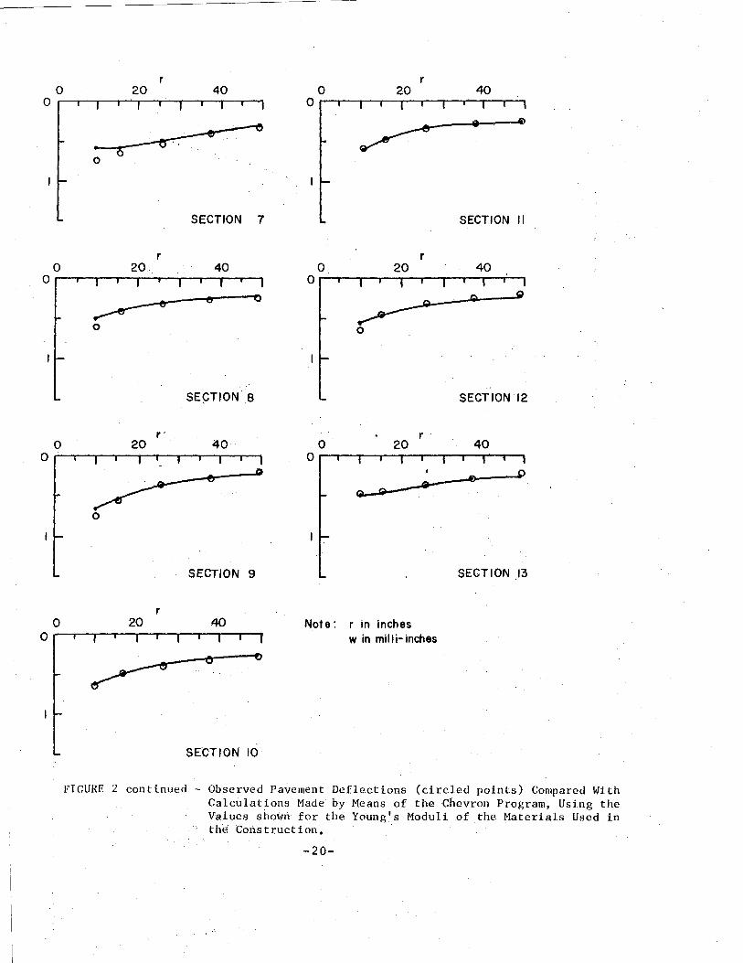
FIGURE 2 continued - Observed Pavement Deflections (circled points) Compared With Calculations Made by Means of the Chevron Program, Usi.ng the Values shown for the Young's Moduli of the Materials Used in the Construction.

-20-

r 0 20 40

0 --~~~~~r-~,--.-.-,

SECTION 14

SECTION 15

SECTION 16

SECTION 17

r

r 20

Note : r in inches w in miiiHnches

SECTION 18

40

SECTION 19

SECTION 20

FIGURE 2 continued -. Observed Pavement Defiections (circled points) Compared With Calculations Made by Means of the Chevron Program, Usiil.g the Values shown. for the. Young's Moduli of the Materials Used in the Construction.

-21-

r r

SECTION 21 SECTION 27

r r

0 0

SECTION 24 SECTION 28

r r

SECTION 25 SECTION 29

r Note; r in inches

w in mi IIi-inches

SECTION 26

FIGURE 2 continued - Observed Pavement Deflections (circled points) Compared With Calculations Made by l'.feans of the Chevron Prog.ram; Using the Values shown for the Young's Moduli of the Materials Used in the Construction.

-22~

0.9 +

0.7

0.6

+ + 0.5

+ ..Q

0.4 +

+ 0.3

+

0.2 +

0.1

10,000 100,000 1,000,000

YOUNG'S MODULUS E (ASSUMING A POISSONS RATIO OF 0 · 45)

' d. A i t the "b 's" FIGURE 3 - Values of the Estimated E s Plotte ga ns

Determined by Scrivner and Moore. -23-

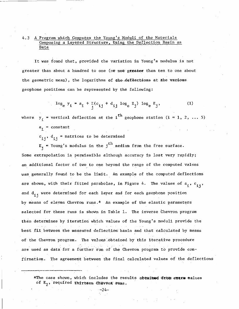
4.3 A Program which Computes the Young's Moduli of the Materials Composing a Layered Structure, Using the Deflection Basin as Data

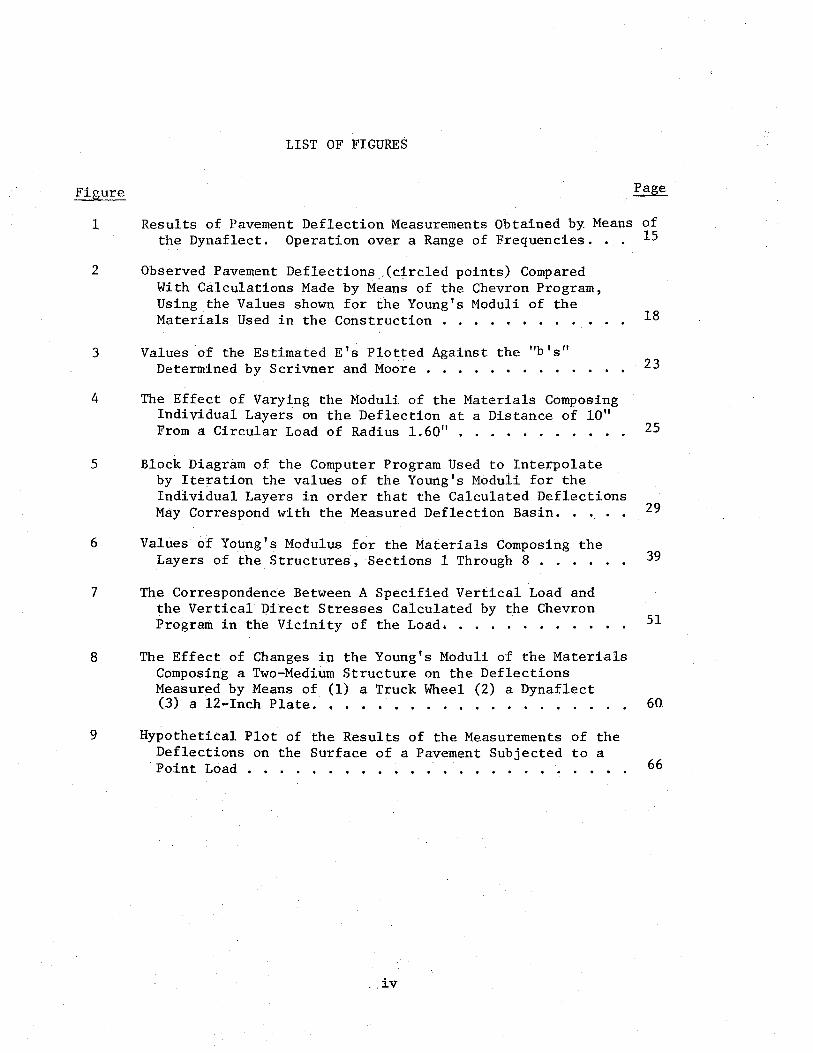
It was found that, provided the variation in Young's modulus is not

greater than about a hundred to one (o~ no~ g£eaner than ten to one about

the geometric mean) , the logarithms of nhe· ~clefilectihoas at the -vard:oas

geophone positions can be represented by the following:

loge yi = ai + rcij + dij loge Ej) loge Ej, (1)

where yi =vertical deflection at the ith geophone station (i = 1, 2, ... 5)

a. = constant 1

cij' dij =matrices to be determined

E. = Young's modulus in the jth medium from the free surface. J

Some extrapolation is permissible although accuracy is lost very rapidly;

an additional factor of two to one beyond the range of the computed values

was generally found to be the limit. An example of the computed deflections

are shown, with their fitted parabolae, in Figure 4. The values of a., c .. , 1 1]

and dij were determined for each layer and for each geophone position

by means of eleven Chevron runs.* An example of the elastic parameters

selected for these runs is shown in Table 1. The inverse Chevron program

then determines by iteration which values of the Young's moduli provide the

best fit between the measured deflection.basin and that calculated by means

of the Chevron program. The values obtained by this iterative procedure

are used as data for a further run of the Chevron program to provide con-

firmation. The agreement between the final calculated values of the deflections

*The case shown, which includes the results n~~iaed ~~~ e~~~ ~alues of E2 , required thir1t@en ebe'V~o1i·ttfins.

-24-

I 9 8 7

6

5

4

3

2

I 9 8 7

6

5

4

3

2

K

I 10,000

)(..,

~

E/ Cl_+ 4 E5

I i 1

i ! !

I I

I I

I I

I

I

I I I !

I ' I

l \ I I I I I

I I I I I I I I i I i ! I

I

I !

I I i I 1 I I I i I !

-[ i I

i i

I

I I

I I

I I

' I

r--.. I

I i ! ......

~ i '

t !") r-. .... I -II -iF1 E'3 ""x I I E/ j

I 2

i i I i

I

I i i

' I I i

I

I

I I !

I I I ! I

! I ! I i I

r I ' ! !

I i I I I I

! I

I I i I !

I I i ' I

I I

! l

I I i I ! I

I '

I I I I

i I 5 100,000 5 1,000,000

YOUNGS MODULUS (LB./IN.2)

FIGURE ·4 - The· Effect of Varying the Moduli of the Materials Composing Individual Lavers on the Deflection. at· a Distance of 10" From a Circul~r Load of Radius 1.60 1 ~.

I

:

! I

I I I

!

I I I I

I !

I i I ! I

l I I ! I l I i I

I I

I I

I i i i

I r I I

I i

I i

I ' '

1-i--L.. ' I I

i I ! I I

! i 1 I

I ! I I ! I I i i I I ! I I

i i ' i I I

I ' i I i I I i I I I

1 ! ! i i i I ! i

; I ' i I i

' I ! i

I i I

I

l I 5

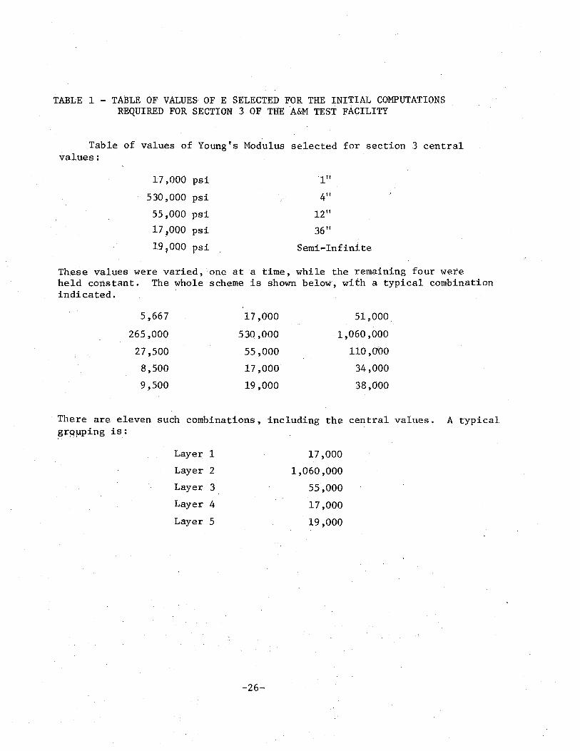
TABLE 1 - TABLE OF VALUES OF E SELECTED FOR THE INITIAL COMPUTATIONS REQUIRED FOR SECTION 3 OF THE A&M TEST FACILITY

Table of values of Young's Modulus selected for section 3 central values:

17,000 psi 1"

530,000 psi 4"

55,000 psi 12"

17,000 psi 36 II

19JOOO psi Semi-Infinite

These values were varied, one at a time, while the remaining four were held constant. The whole scheme is shown below, with a typical combination indicated.

5,667 17,000 51,000

265,000 530,000 1,060,000

27,500 55,000 110,0'00

8,500 17,000 34,000

9,500 19,000 38,000

There are eleven such combinations, including the central values. A typical ~:J:"QJ.Jping is:

Layer 1 17,000

Layer 2 1,060,000

Layer 3 55,000

Layer 4 17,000

Layer 5 19,000

-26-

--- - -------- ~-~-~~· ----

and those measured in the field indicates the sufficiency of the model

represented by equation 1. Greater accuracy could be achieved by employing

terms of the third order in log E., or by intrJoddcing terms involving cross J

products of the log E.'s. Comparison between the final calculated and J . . R

the observed values of the deflections shows the agreement is better than

a unit in the least significant digit in the measured values. The accuracy

achieved by means of the present expression is adequate.

-27-

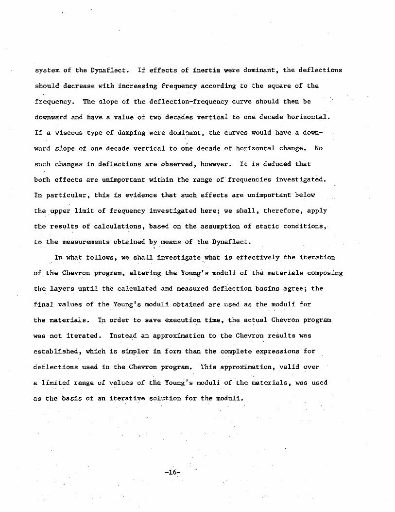
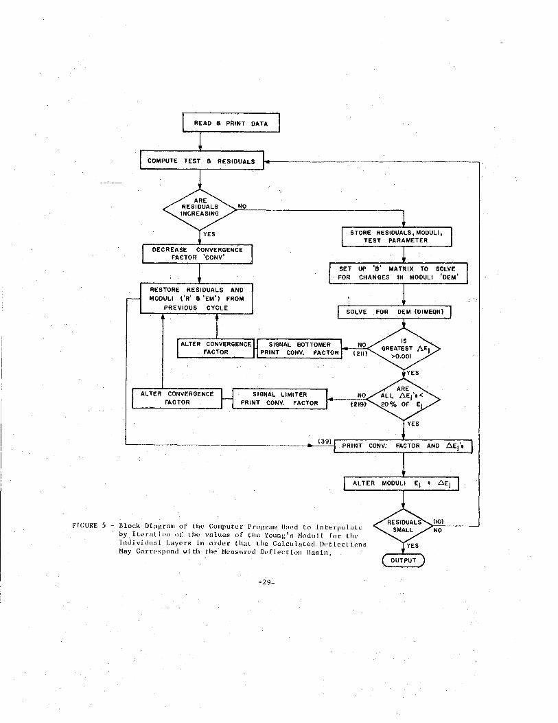
4.3.1 Description of the Pr<;>gram

A block diagram of the main routine of_ the convergence program WHC36

is shown in Figure 5. The program consists of a main routine and two

subroutines DIMEQN and COEFFT. DIMEQN is a subroutine which inverts a

matrix, and is used to solve five simultaneous equations; COEFFT is a

subroutine which calculates the elements of the matrices C(I,J) and

D(I,J) using as input data the grid of values of deflections Y(1,J)

which are calculated by means of the Chevron program.

The program operates as follows.- The vector A(I) and the matrices

C(I,J) and D(I,J) are calculated as described. The trial values of E(J)

are used to calculate the Y(I) vector. The calculated Y vector is

subtracted from the measured Y vector. The result, the R vector, is

used in the following set of simultaneous equations:

(C(l,l)+2*D(l,l)*EM(l))*DELTA(EM(l))+ ••.

••• +C(l,J)+2*D(l,J)*EM(J))*DELTA(EM(J))=-R(l)

(C(J ,1)+2*D(J ,1) *EM(J) *DELTA(EM(J) )+ •••

.•. +(C(J,J)+2*D(J,J)*EM(J)*DELTA(EM(J))=-R(J),

which are solved for DELTA (EM(K)), (K = 1, •• ,J) the correction to be

applied to EM(K), the logarithm of Ek. On the first cycle of iteration,

the trial E vector is placed in the EM(K)'s, and the change DELTA(EM(K))

in the EM(K)'s is calculated which is necessary to make the R vector zero,

i.e. to make the calculated Y's agree with the measured Y's. A fraction of

the calculated changes in the EM(K) 's is added•.' to1;the trial· values .of, EM.(K} -~,

-28-

COMPUTE TEST 8 RESIDUALS r-----------------------..,

No

DECREASE CONVERGENCE FACTOR 'CONV'

RESTORE RESIDUALS AND MODULI ( 'R' 8 'EM') FROM

PREVIOUS CYCLE

SIGNAL BOTTOMER PRINT CONV.

ALTER CONVERGENCE FACTOR

SIGNAL LIMITER PRINT CONV. FACTOR

SET UP '8' MATRIX TO SOLVE FOR CHANGES IN MODULI 'OEM'

SOLVE FOR

~--------------------------------------.__ll_g~)r--PR_I_N_T __ C_O_N_V_: __ F_A~C-TO_R ___ A_N_D--~~EJ7'a-,

ALTER MODULI Ej t 6Ej

FLGURE 5 - Block Dingram of the Con~uter Program Used to Interpolate by Itcratlon ,,r the values of the Young's Moduli for the lndl viduaL Lnyc rs in order that the Cal.cu luted Deflections May Correspond with the Measured Deflettion Basin,

-29:...

and the operation is repeated, until the solution criterion is satisfied.

It is necessary to use only a small fraction of the calculated changes

in the EM(K)'s as a correction to the trial EM(K)'s in order to prevent

oscillation. Other safeguards were included, such as discontinuing the

program when the changes in the calculated Y become too small, and also

when some varieties of saddle point are reached.

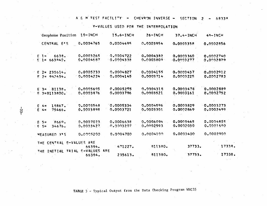
The input data are complicated, and a program has been written (WHC35)

in order to assist with checking it for numerical and sorting errors. The

input data are as shown in Table 2. A typical output from the checking

program is shown in Table 3.

Normal functioning of the program leads to values of EM(K)'s for the

materials composing the layers; the values yield the correct deflections

(those measured in the field)wwhen used as input data to the Chevron

program. If the·discrepancies are larger than the errors of the observed

(field) deflections, then the program is hot functioning properly. See

the section concerning fault tracing.

-30-

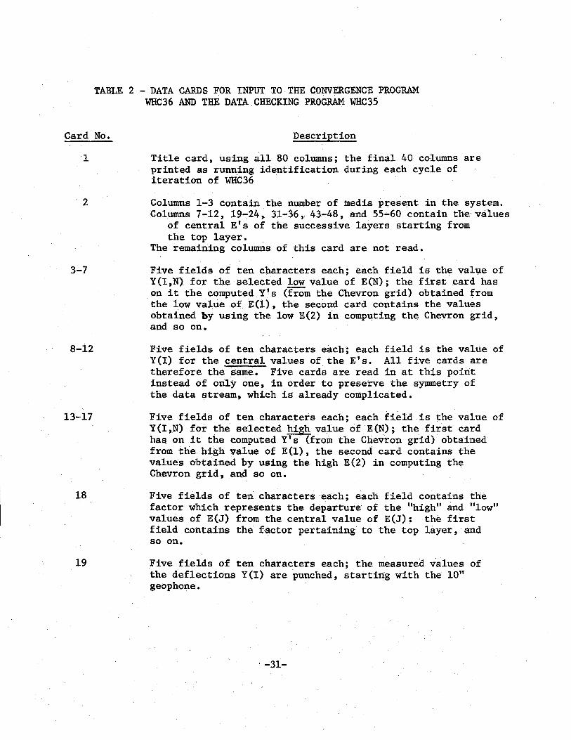
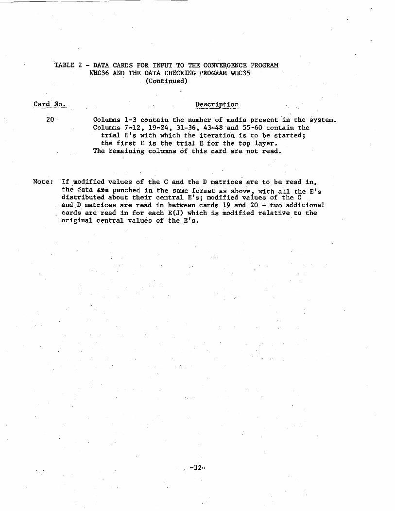
TABLE 2 - DATA CARDS FOR INPUT. TO THE CONVERGENCE PROGRAM WHC36 AND THE DATA CHECKING PROGRAM WHC35

Card No. Description

1

2

3-7

8-12

13-17

18

19

Title card, using all 80 columns; the final 40 columns are printed as running identification during each cycle of iteration of WHC36

Columns 1-3 contain the number of media present in the system. Columns 7-12, 19-24, 31-36, 43-48, and 55-60 contain theva1ues

of central E's of the successive layers starting from the top layer. .

The remaining columns of this card are not read.

Five fields of ten characters each; each field is the value of Y(I,N) for the selected low value of E(N); the first card has on it the computed Y's (from the Chevron grid) obtained from the low value of E(l), the second card contains the values obtained by using the low E(2) in computing th~ Chevron grid, and so on.

Five fields of ten characters each; each field is the value of Y(I) for the central values of the E's. All five cards are therefore the same. Five cards are read in at this point instead of only one, in order to preserve the symmetry of the data stream, which is already complicated.

Five fields of ten characters each; each field is the value of Y(I,N) for the selected hiSh value of E(N); the first card has on it the computed Y's (from the Chevron grid) obtained from the high value of E(l), the second card contains the values obtained by using the high E(2) in computing the Chevron grid, and so on.

Five fields of ten characters each; each field contains the factor which represents the departure of the "high" and "low" values of E(J) from the central value of E(J): the first field contains the factor pertaining to the top layer, and so on.

Five fields of ten characters each; the measured values of the deflections Y(I) are punched, starting with the 10" geophone.

'..;31-

----------------------------

TABLE 2 - DATA CARDS FOR INPUT TO THE CONVERGENCE PROGRAM WHC36 AND THE DATA CHECKING PROGRAM WHC35

(Continued)

Card No. Description

20 Columns 1-3 contain the number of media present in the system. Columns 7-12, 19-24, 31-36, 43-48 arid 55-60 contain the

trial E's with which the iteration is to be started; the first E is the trial E for the top layer.

The remaining columns of this card are not read.

Note: If modified values of the C and the D matrices are to be read in, the data •re punched in the same format as above, with all the E's distributed about their central E's; modified values of the C and D matrices are read in between cards 19 and 20 - two additional cards are read in for each E(J) which is modified relative to the original central values of the E's.

I -32-

A ~ M TEST FACILITY CHEVR')N INVERSE - SECTION 2 6833~

Y-VALUES USED FOR THE INTERPOLATION

Geophone Position 10-INCH 15.6- INCH 26-INCH 37.4-INCH 49·..YNCH

CENT~AL E'S 0.0004765 0.000449~ 0.1)003954 0.00033~A 0.00028.56

E 1= 66'38. 0.0003265 0.1)004722 0.0004382 0.0003360 0.0002740 '= 1= 663~40. 0.()004687 0.01)0433~ 0.0003809 0.01')03277 o.o0o2a~<:l

E 2= 235614. 0.0005233 0.0004827 0.0004155 o. 00034.3 7 0 .• 0002912 f. 2= <:l42454. 0.0004224 0.0004145 0.0003714 0.0003225 0.0002783

..

E 3: 81138. 0.0005695 0.0005255 0.00043!8 0.0003478 0.0002889 E 3=8113800. 0.0003876 0;.0003796 0.0003521 0.0003161 0.0002752

E 4= 18867. 0.0005548 0.0005334 0.00045<)6 0.0003829 0.0003273 I

E 75466 •. o.ono3898 0.0003721 0.0003301 0.0002869 0.0002499 VJ 4= VJ I

E 5= 8669. 0.00070~3 0.0006638 0.0006094 0.0005465 0.0004855 f 5= 346 76. 0.0003427 n.QOf')3207 0.0002593 0.0002030 0.')0016<:10

MEASURED v•s 0.0005200 0.0004700 0.0004100 0.0003400 0.0002900

THE CENTRAL E-VALUES A~E 663$34. 471227. 811380. 37733. 17338.

THE INITIAL TRIAL F.-VALUES A~E

66384. 235613. 811380. 31733. 17338.

TABLE 3 - Typical Output from the Data Checking Program WHC35

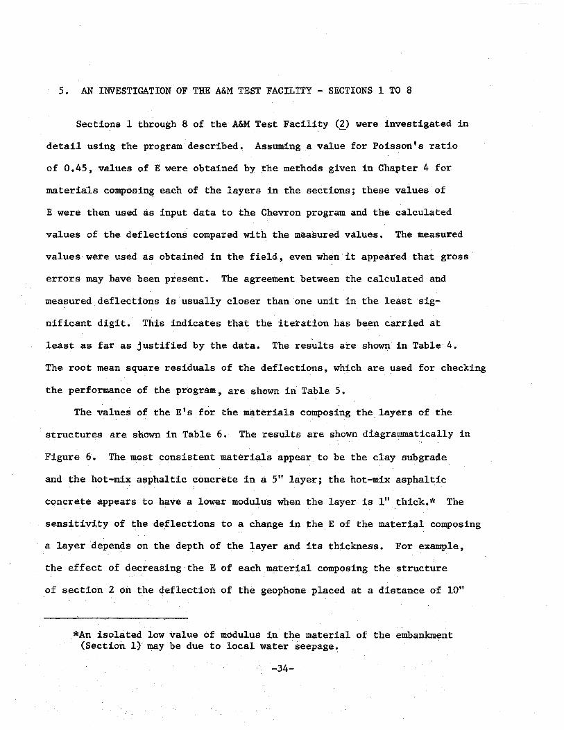
5. AN INVESTIGATION OF THE A&M TEST FACILITY - SECTIONS 1 TO 8

Sections 1 through 8 of the A&M Test Facility (2) were investigated in

detail using the program described. Assuming a value for Poisson's ratio

of 0.45, values of E were obtained by the methods given in Chapter 4 for

materials composing each of the layers in the sections; these values of

E were then used as input data to the Chevron program and the calculated

values of the deflections compared with the measured values. The ~easured

values were used as obtained in the field, even when it appeared that gross·

errors may have been present. The agreement between the calculated and

measured deflections is usually closer than one unit in the least sig-

nificant digit. This indicates that the iteration has been carried at

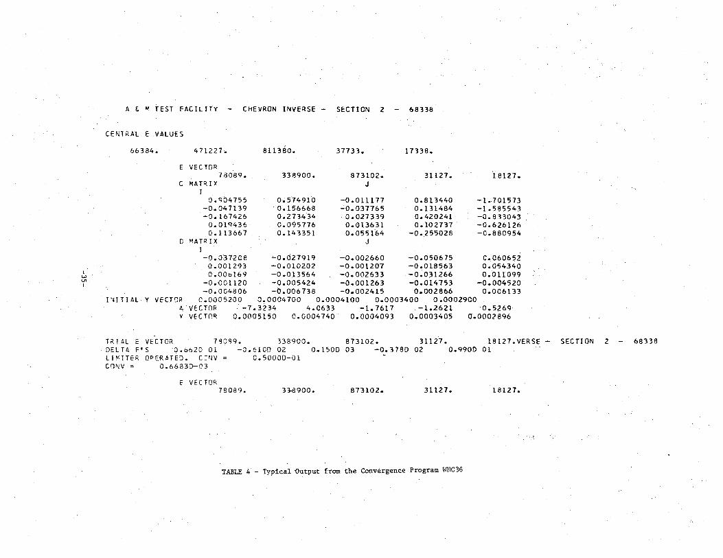
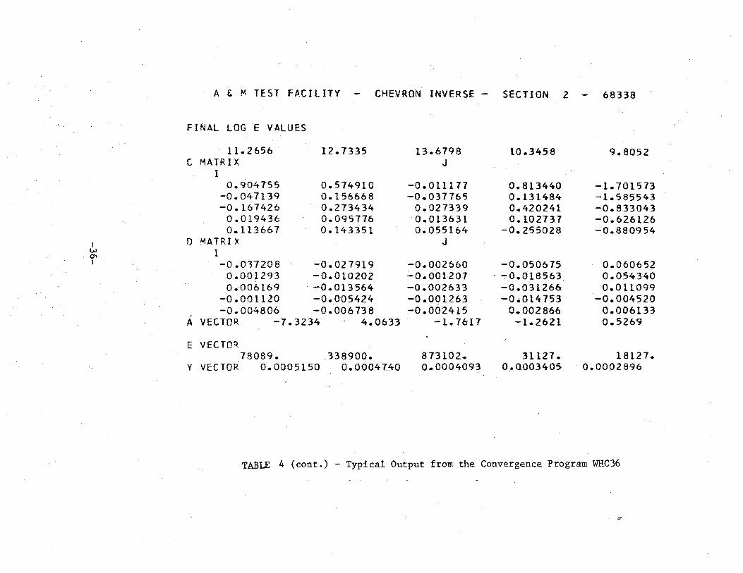
least as far as justified by the data. The results are shown in Table 4.

The root mean square residuals of the deflections, which are used for checking

the performance of the program, are shown in Table 5.

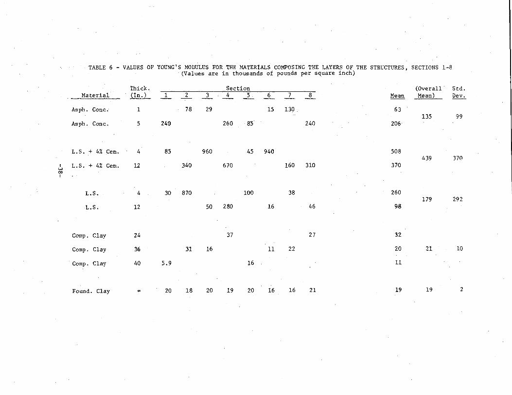
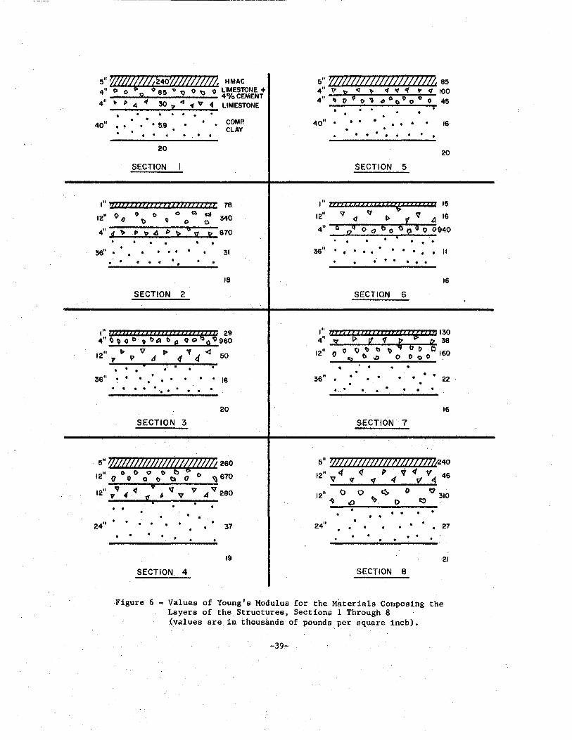
The values of the E's for the materials composing the layers of the

structures are shown in Table 6. The results are shown diagrammatically in

Figure 6. The most consistent materials appear to be the clay subgrade

and the hot-mix asphaltic concrete in a 5" layer; the hot-mix asphaltic

concrete appears to have a lower modulus when the layer is 1" thick.* The

sensitivity of the deflections to a change in the E of the material composing

a layer depends on the depth of the layer and its thickness. For example,

the effect of decreasing the E of each material composing the structure

of section 2 on the deflection of the geophone placed at a distance of 10"

*An isolated low value of modulus in the material of the embankment (Section 1) may be due to local water seepage.

-34-

I ...., \J1 I

A fi ~TEST FACILITY - CHEVRON INVERSE- SECTION 2 68338

CE~TRAL E VALUES

!>6 3 84. 471227.

E VECTOR 78089.

C MATtl.lX I

0.904755 -0.047139 -0.167426

0.019436 0.113667

G ~ATRIX I

811380.

338900.

0.574910 0.156668 0.273434 0.095776 0.143351

-0.037208 -0.027919 0.001293 -0.010202 O.DOal69 -0.013564

-O.D01120 -0.005424 -0.004806 -0.006738

37733.

873102. J

-o .011111 -0.037765

0.027339 0.013631 0.0551.64

J

17338.

31127.

0.813440 0.131484 0.420241 0.102737

-0.255028

-0.002660 -0.050675 -0.001207 -0.018563 -0.002633 -0.031266 -0.001263 -0.014753 -0.002415 0.002866

18127.

-1.701573 -1.585543 -o. 8 33043 -0.626126 -0.880954

0.060652 0.054340 0.011099

-0.004520 0.006133

I,ITIAL Y VECTOR 0.0005200 0.0004700 A'VECTOR -7.3234

0.0004100 0.0003400 0.0002900

Y VECTn~ 0.0005150

TK 1 AI.. E VECTOR 7'30'l9.

4.0633 -1.7617 ~1.2621

0.0004740 0.0004093 0.0003405

338900. 873102. 31127.

0.5269 0.000?896

18127.VERSE-DEL H F'S 0.6620 01 -0.610[) 02 0.1500 03 -o.:n8o 02 0.9900 01 Ll"'lTER OPERATED. c:~N 0.50000-01 -C<JI.;V = 0.66830-03

f VECTOR 78089. 33-8900. 873102. 31127. 18127.

TABLE 4 - Typical Output from the Convergence Program ~~C36

SECTION 2 68338

A & M TEST FACILITY CHEVRON INVERSE - SECTION 2 68338

FINAL LOG E VALUES

11.2656 12.7335 13.6798 10.3458 9.8052 c MATRIX J

I 0.904755 0.574910 -0.011177 0.813440 -1.7015 73

-0.047139 0.156668 -0.037765 0.131484 -1.585543 -0.167426 0.273434 0.027339 0.420241 -0.833043

0.019436 0.095776 0.013631 0.102737 -0.626126 0.113667 0.143351 0.055164 -0.255028 -0.880954

I D MATRIX J w I 0\ I -0.0~7208 -0.027919 -0.002660 -0.050675 0.060652

0.001293 -0.010202 .;_0. 001207 ' -0.018563 0.054340 0.006169 -0.013564 -0.002633 -0.031266 0.011099

-0.001120 -0.005424 -0.001263 ---o.ol4753 -0.004520 -0.004806 -0.006738 -0.002415 0.002866 0.006133 .

A VECTOR -7.3234 4.0633 -1.7617 -1.2621 0.5269

E VECTOQ. 78089. 338900. 873102. 31127. 18127.

y VECTOR 0.0005150 0.0004740 o.ooo4093 0.0003405 0.0002896

TABLE 4 (cont.) - Typical Output from the Convergence Program WHC36

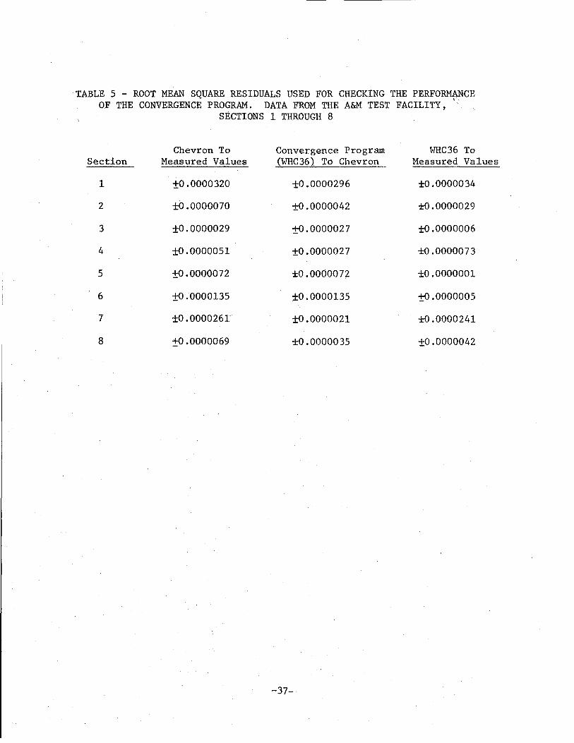
TABLE 5 - ROOT MEAN SQUARE RESIDUALS USED FOR CHECKING THE PERFORMANCE t'•

OF THE CONVERGENCE PROGRAM. DATA FROM THE A&M TEST FACILITY, SECTIONS 1 THROUGH 8

Chevron To Convergence Prbgram WHC36 To Section Measured Values (WHC36) To Chevron Measured Values

1 ±0.0000320 ±0.0000296 ±0.0000034

2 ±0.0000070 ±0.0000042 ±0.0000029

3 ±0.0000029 ±0.0000027 ±0.0000006

4 ±0.0000051 ±0.0000027 ±0 .0000073

5 ±0 .0000072 ±0 .0000072 ±0.0000001

6 ±0.0000135 ±0.0000135 ±0.0000005

7 ±0.0000261 ±0.0000021 ±0.0000241

8 ±<L0000069 ±0.0000035 ±0.0000042

-37-

I w (X)

I

TABLE 6 -VALUES OF YOUNG'S MODULUS FOR THE MATERIALS COMPOSING THE LAYERS OF THE STRUCTl~ES, SECTIONS 1-8 (Values are in thousands of pounds per square inch)

Thick. Section (Overall Std. Material (In.) 1 2 3 4 5 6 7 8 Mean Mean) Dev.

Asph. Cone. 1 78 29 15 130 63 135 99

Asph. Cone. 5 24:0 260 85 240 206

L.S. + 4% Cern. 4 85 960 45 940 508 439 370

L.S. + 4% Cern. 12 340 670 160 310 370

L.S. 4 30 870 100 38 260 179 292

L.S. 12 50 280 16 46 98

Comp. Clay 24 37 27 32.

Cornp. Clay 36 31 16 11 22 20 21 10

Cornp. Clay 40 5.9 16 11

Found. Clay "' 20 18 20 19 20 16 16 21 19 19 2

5" @Jfl(lll124oV)IftiiJ/Z HMAC 4" Q o 0 85 9 ~ o ~ 9 LIMESTONE +

o 4%CEMENT 4" .- • 4 4 30 t 4 ~ V 4 LIMESTONE

4011 .. • • 5.9 . . 20

SECTION

. . • •

COMP. CLAY

1" uzzzzzzzzzzzzzzzzlzzzzzzzz 78 0 0 <> ~

1211 00 \) 0 0

4" ~ " I> 2;4 l> k . 36" . . ••

• . •

SECTION 2

1211 ,. . . .

36" •• . . . . . . . . SECTION 3

Sl

. .

c=J 0

340

IZ 870

• 31

18

• 16

20

s" W)llj/J/7Jf//l/ll{(l !1/li 260

1211 0 I> () I> b 0 670 (10QC)t)0 ~

12" v "q 4 ill ' • tq v v 4 v 280 ll, . .

24" . . 37

19

SECTION 4

5" zm;]llllllllllJIW/1, 85 4" \)" 'ljr 4 ~ ~ ., "( ~ ~ 100 4" ~ t> 6 0 '\\ ~ Q Ct 0 0 '\) 0 45 . .

40" • • • • • • 16 . . • • •

20

SECTION 5

1" z z z z z z z z z rz z z z z z f$' z z t t '.I" 1~

1211 v <;f v 16 <1 t> 1 .d 4" 0

0 d o a 6 o ~ o o o 0940 . . . 36" • . . • • • • • II .- . . . . .

16

SECTION 6

" I yzzzzzzzzzzzzzzzzzzz'Jzzzz.130 4

11 y t'> V' 1 ~ {) 38

12" 0 I? Q ~ ll ~ 6 " . t3 160 9 «>.o OOoO

.. 36" . .

16

SECTION 7

5" lfiWl/ll//WdWZWv240 1211 4 <1 P' v <( v 46 v v '(/ 4 'ff 4

1211 () 0 ~ 0 'i7 310 ~ !(;) lb 0 co

• . • . 2411

27 . • 21

SECTION 8

Figure 6 - Values of Young's Modulus for the Materials Composing the Layers of the Structures, Sections 1 Through 8 (values are in thousands of pounds per square inch).

-39-

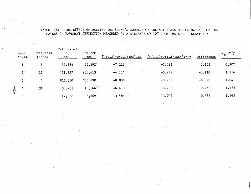
from the load can be calculated; this is done by means of the elements

C(l,J) and D(l,J) for values of J from one to five. The results are

shown in Table 7(a). Decreasing the Young's modulus of the material

composing the top layer (the hot-mix asphaltic concrete) actually

decreases the deflection at a distance of 10"--in all other cases the

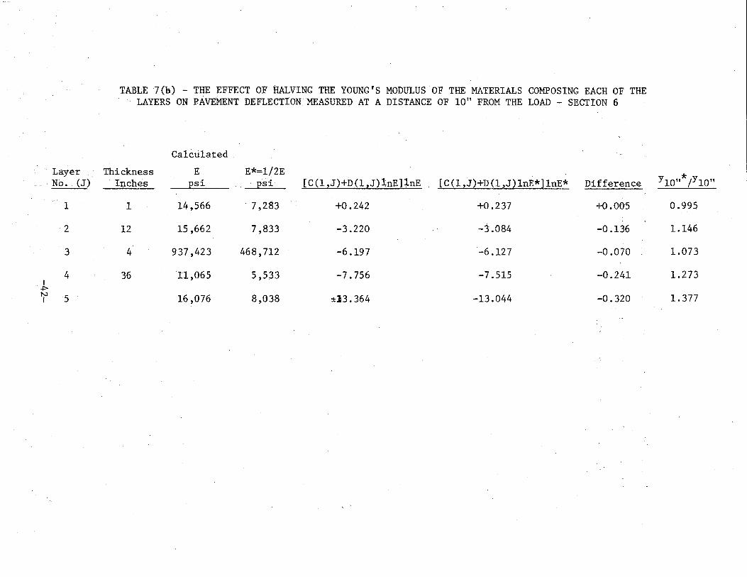
deflection is increased. Section 6 has the same thickness distribution

and placement of the layers but hhe moduli of all the materials except

that composing the subgrade are different from those. composing the structure

of Section 2. Table 7(b) shows that a decrease in the E of the top layer

of Section 6 leads to a decrease in the deflection measured at ten inches

from the load; decreases in the moduli of any of the materials composing

the other layers leads to an increase in the value of this deflection.

'This is qualitatively the same as in the case of Section 2.

The corresponding ratios obtained using the deflections at 49" from

the load are as follows:*

Section 2:

Section 6:

Layer 1

0.988,

0.997,

Layer 2

1.019'

0.919,

Layer 3

m. !198,

0.998,

Layer 4

1.156'

1.191'

Layer 5

1.696

1.839

These figures indicate that the 49" deflection is relatively sensitive to

changes in the moduli of the material composing the subgrade; the sensitivity

decreases for the upper layers.

By comparing the figures above with those in Tables ~(a) and ~(b), it

can be seen that the deflection of the 1011 geophone is less sensitive than

*The meaning of these figures is, for example, "The ratio of the 49" defJ_ection for '·half the calculated value of E (5) in Section 2 to the deflection for the calculated value of E (5) is 1. 696".

-40-

Layer No. (J)

1

2

3

I 4 ~ 1-' I

5

TABLE 7(a) - THE EFFECT OF HALVING THE YOUNG'S MODULUS OF THE MATERIALS COMPOSING EACH OF THE LAYERS ON PAVE:IYIENT DEFLECTION MEASURED AT A DISTANCE OF 10" FROH THE LOAD - SECTION 2

Calculated ';rhickness E E*=l/2E

Inches psi psi . [C(l,J)+D(l,J)lnE]lnE [C(l,J)+D(l,J)lnE*]lnE* Difference

1 66,384 33,192 +7 .116 +7.013 0.103

12 471,227 235,613 -4.054 -3.944 -0.110

4 811,380 405,690 -0.808 -0.768 -0.040

36 36 '733 18,366 -6.490 -6.236 -0.253

17,338 8,669 -13.586 . -13.202 -0.384

ylO"*/ylO"

0.902

1.116

1.041

1.288

1.468

Layer No. (J)

1

2

3

4 I ~ N 5 I

TABLE 7 (h) - THE EFFECT OF HALVING THE YOUNG'S MODULUS OF THE MATERIALS COMPOSiNG EACH OF THE LAYERS ON PAVEMENT DEFLECTION MEASURED AT A DISTANCE OF 10" FROM THE LOAD - SECTION 6

Calculated

Thickness E E*=l/2E Inches psi psi [ C (1 ,J)+D(l ,J) lnE]lnE [ C (1 ,J)+D (1 ,J) .lnE*] lnE* Difference

1 14,566 7,283 +0.242 +0.237 +0.005

12 15,662 7,833 -3.220 -3.084 -0.136

4 937,423 468 '712 -6.197 -6.127 -0.070

36 11,065 5,533 -7.756 -7.515 -0.241

16,076 8,038 ~13.364 -13.044 -0.320

Yl011*/yl0"

0.995

1.146

1.073

1.273

1.377

the deflection of the 49" geophone to changes in the subgrade modulus.

Both the 10" and the 49" geophone are relatively insensitive to changes

in the moduli of the upper three layers.

-:-43-

5.1 Conclusion

The need exists to determine the elastic moduli of the materials

composing the structure of a highway pavement. The knowledge of the

moduli provides a means of calculating the stresses in the subsurface

layers caused by loads on the surface. In this part of the report a

method of estimating the required moduli from the measured surface

deflections has been discussed. The surface deflections were obtained

from the results of measurements made by means of the Dynaflect apparatus,

discussed in Chapter 2. A deflection basin, as determined by elastic

theory, was fitted to the measured deflections. When a good fit was

achieved, the values of the elastic parameters were assumed to be those

of the materials composing the pavement structure.

The loading system of the Dynaflect may be a cause of significant

error. Owing to resonances in the Dynaflect chassis, it is likely that

the load actually applied to the pavement is less than calculated from

the simple dynamics of the loading system. The elastic moduli for the

materials would then be lower than those obtained here.

-44-

5.2 Suggestions for Further Work

The work reported herein suggests the desirability of certain

further work.

-45-

5.2.1 Improving the Accuracy of the Moduli of the Materials Composing The Layers Nearest to the Surface

It is a weakness of the present work that the moduli of the materials

composing the layers close to the surface cannot be found with accuracy;

this is evidenced by the elements of the C and D matrices relating to

these layers - large changes in the moduli of the materials composing

the layers lead to only small changes in the measured points of the

deflection basin. The changes in the moduli of the deeper layers have,

however, an appreciable effect on the measured deflections. Generally

it appears that the effectiveness of a change in modulus at depth d is

a maximum at a spacing of approximately d.

In order, therefore, to determine accurately the moduli of the

materials within the layers close to the surface, basin points should

be determined at spacings much smaller than those so far employed. The

program discussed here is directly applicable if shorter spacings are

used. The matrix elements will, however, be such that the measured

deflections will have a far greater influence on the values of the

surface moduli than is at present the case.

-46...:

5.2.2 Extension of the work in order that the loading conditions may correspond with those induced by traffic

The deflection basins could be measured over a range of frequencies

up to the highest of those which occur due to traffic loading. This

will enable the moduli to be determined under conditions which are more

truly representative of the actual traffic loading conditions. If this

were done, inertia and damping would· probably have to be taken into

account. The Chevron program used in the present work would not neces-

sarily be adequate as a confirmation for trial values of the moduli.

A program which could be adapted for use under these conditions will

be discussed in Part 2 of this peport.

-47-

; ' APPENDIX A - THE OPERATION OF THE CHEVRON PROGRAM

-48-

-------------------------------------------------------------------------------------

A.l The Accuracy of the Chevron Program

The following are two main causes of error in the results obtained

from the Chevron program. The accuracy of the Bessel function in the

subroutine BESSEL may be insufficient; this can be improved if required

by taking additional terms in the numerical integration. Second, the

number of terms ITN of Bessel functions used to approximate the applied

load can be increased. This is set at 46, and any increase would lead

to an increase in execution time in proportion to ITN, as the integration

is the major operation of the program. The accuracy is probably better

than the 5% claimed by the authors, as shown by the following checks.

-49-

------------------------~----------------

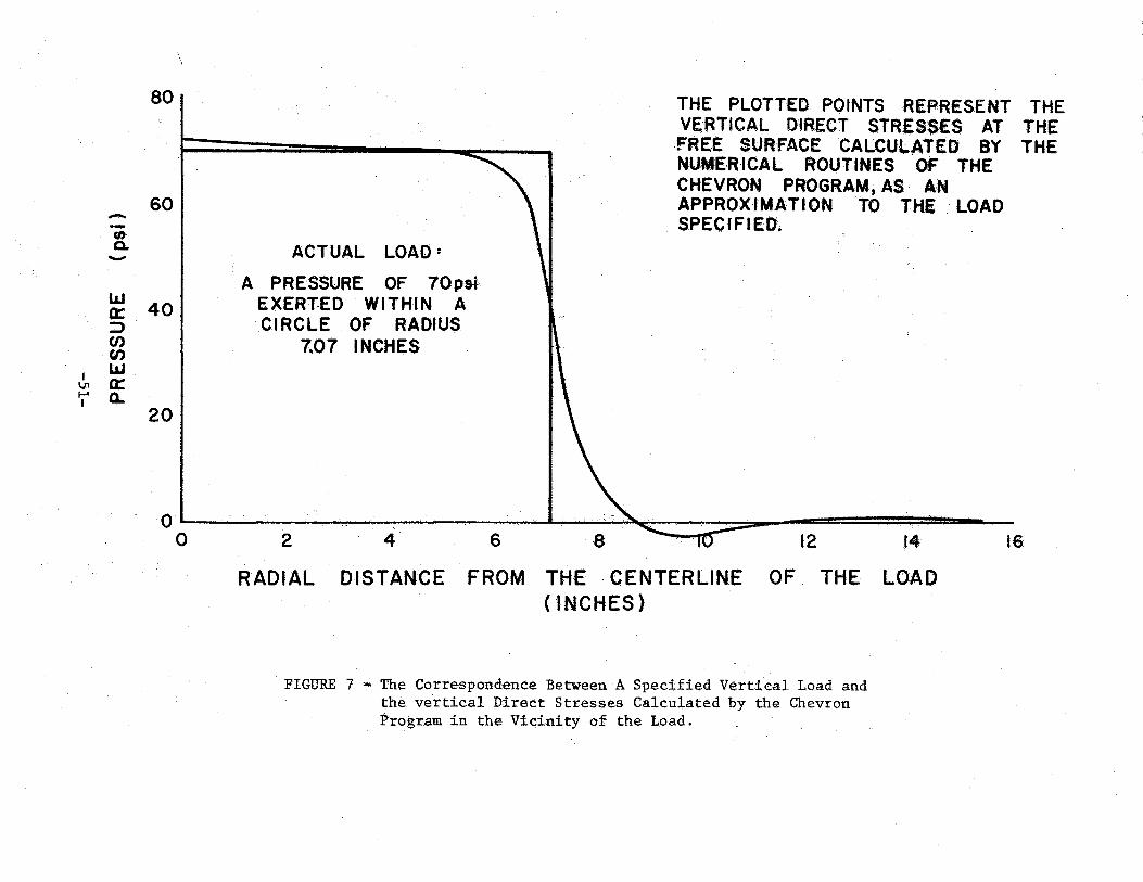
_A.l.l The Accuracy of Representing the Applied Load

The Chevron program was used to calculate the vertical direct

st.resses at the free surface of a semi-infinite medium, loaded by means

of a circular load with a radius of 7.07 inches and exerting a constant

pressure over the loaded area of 70 pounds per square inch. The results

of the calculations are shown in Figure 7. The figure shows the actual

load represented by a rectangle, and the approximation to it represented

by fl 1 smootih:'aarte. It appears that the accuracy of ·the ealculat:lqns b

sufficient for almost all engineering purposes.

-50-

--(I)

Q. -LaJ a: :::> en (,/)

I LIJ \J1 a:: 1-' a.. I

80

60

A

40

20

ACTUAL LOAD:

PRESSURE OF 70psl EXERT-EO WITHIN A CIRCLE OF RADIUS

7.07 INCHES

THE PLOTTED POINTS REPRESENT THE VERTICAL DIRECT STRESSES AT THE FREE SURFACE CALCULATED BY THE NUMERICAL ROUTINES OF THE CHEVRON PROGRAM; AS AN APPROXIMATION TO THE . LOAD SPECIFIED.

oL-~~--~~----~~--~~~~~----~----=========----0 2 4 6 8 12 14 16

RADIAL DISTANCE FROM THE ·CENTERLINE OF THE LOAD (INCHES)

FIGURE 7 "" The Correspondence Between A Specified Vertical Load and the. vertical Direct Stresses Calculated by the Chevron Program in the Vicinity of the Load.

A.l.2 The Accuracy of Representing the Vertical Settlements at the Free Surface

The accuracy of representing the vertical settlements at the free

surface is less easy to establish, because it is less easy to determine

what these should be. However, certain closed solutions are available

which may be used to check in a limited way the results of the Chevron

computations. Biot (14) has determined the stresses within an elastic

layer bounded by a rigid $Urface at its base. These results were

presented in a more general form by Pickett (15). The stresses in such

systems were expressed by means of integrals which can be evaluated by

approximate methods or by numerical integration. As a check on the

accuracy of the vertical settlements calculated by means of the Chevron

program, it is suggested that the Boussinesq solution should be used;

the spacing should be large compared with the radius of the loaded

circle for which the Chevron calculations are made. Table 8 is an

example of the use indicated.

The results given in Table 8 indicate that the calculations made

by means of the Chevron program are probably accurate to 5% or less

within a spacing equal to ten radii of the applied load; the accuracy

is better at small spacings than at large spacings.

-52-

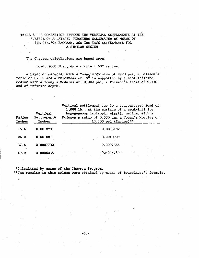
TABLE 8 - A COMPARISON BETWEEN THE VERTICAL SETTLEMENTS AT THE SURFACE OF A LAYERED STRUCTURE CALCULATED BY MEANS OF

THE CHEVRON PROG"AAM, AND THE TRUE SETTLEMENTS FOR A SlMILAR SYSTEM

The Chevron calculations are based upon:

Load: 1000 lbs., on a circle 1.60" radius.

A layer of material with a Young's Modulus of 9990 psi, a Poisson's ratio of 0.330 and a thickness of 18" is supported by a semi-infinite medium with a Young's Modulus of 10,000 psi, a Poisson's ratio of 0.330 and of infinite depth.

Vertical Radius Settlement* Inches Inches

15.6 0.001823

26.0 0.001081

37.4 0.0007730

49.0 0.0006035

Vertical settlement due to a concentrated load of 1,000 lb., at the surface of a semi-infinite homogeneous isotropic elastic medium, with a

Poisson's ratio of 0.330 and a Young's Modulus of l<r;ooo psi (Inches)**

0.0018182

0.0010909

0.0007666

0 .(Ji005789

*Calculated by means of the Chevron Program. **The results in this column were obtained by means of Boussinesq's formula.

-53-

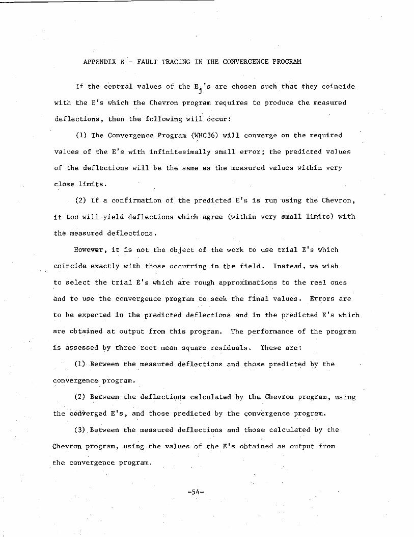
APPENDIX B - FAULT TRACING IN THE CONVERGENCE PROGRAM

If the central values of the E.'s are chosen such that they coincide J

with the E's which the Chevron program requires to produce the measured

deflections, then the following will occur:

(1) The Convergence Program (WHC36) will converge on the required

values of the E's with infinitesimally small error; the predicted values

of the deflections will be the same as the measured values within very

close limits.

(2) If a confirmation of the predicted E's is run using the Chevron,

it too will yield deflections which agree (within very small limits) with

the measured deflections.

However, it is not the object of the work to use trial E's which

coincide exactly with those occurring in the field. Instead, we wish

to select the trial E's which are rough approximations to the real ones

and to use the convergence program to seek the final values. Errors are

to be expected in the predicted deflections and in the predicted E's which

are obtained at output from this program. The performance of the program

is assessed by three root mean square residuals. These are:

(1) Between the measured deflections and those predicted by the

convergence program.

(2) Between the deflections calculated by the Chevron program, using

the corlverged E's, and those predicted by the convergence program.

(3) Between the measured deflections and those calculated by the

Chevron program, using the values of the E's obtained as output from

the convergence program.

-54-

If the program does not perform well, its faults may be diagnosed

by reference to those three root mean square residuals. See TableS.

First, there must be good agreement between the measured deflections

and those predicted by the convergence program. The extent of this

agreement is shown by comparing the Y - vector obtained at the final

cycle of iteration with the "INITIAL Y VECTOR" which is printed before

iteration conunences. See Table 4. If the root mean square residual between

those two sets of Y's is greater than the experimental error of the measured

deflections, i.e. if the predictions are less accurate than the experimental

results, there are two possible causes:

(a) The central E's may have been chosen too far from those E's which

the Chevron program requires to yield the measured deflections. In a very

bad case of this error, in which the error is more than 20% of the measured

deflections, the solution is to use the predicted values of the E's (the

E's obtained as the result of the iteration) as central values for a new

grid of calculations--in other words, to start again.

(b) The iteration may have reached a saddle point, rather than a

true minimum. If this is the case, one or more of the values of E is

incorrect; the process can be continued by providing a trial E which is

more nearly the true one, a decision requiring engineering judgement.

The mean square error at this stage must be made small before any

further fault tracing is undertaken.

Second, there should be good agreement between the deflections

predicted b¥ the convergence program and those calculated by the Chevron

-55-

program. If this is not the case, the fault is assumed to be in the

convergence ptogram and must be due to the inherent inaccuracies of the

logarithmic model which is employed. To correct the fault, one of the

following improvements may be made.

B.l First Operational Suggestion

One or more of the factors governing the choice of the "high E"

and the "low E" are incorrect. These factors may be either too high,

causing the convergence program to calculate a model which does not

represent the actual effect produced by the variation of the particular

E; this case occurs particularly when attempting to find the value of

E in the top layer--a change in the factor often alters the concavity

of the particular element of the model from upwards to downwards, or

the other way round. The factors may be too low, forcing the convergence

program to select E's which are outside the calculated grid, i.e. forcing

extrapolation. The allowable extrapolation depends on the accuracy required.

It seems advisable to reject extrapolations outside a factor of two beyond

the calculated grid. This type of error can be corrected by altering the

factor, and recalculating the portion of the grid affected by means of the

Chevron program. To be sure that this fault is eliminated, the predicted

E should be near a grid point but see the following operational suggestion.

B.2 Second·Operational Suggestion

If a particular E is outside the calculated Chevron grid, it is possible

to converge upon the correct value without recalculating the complete grid.

This may he done as follows. Use the Chevron program .. to. !ctalOJiJtate . :tlrree' ·sets of

--56-

Y's, centered on the expected value of E for the particular layer.

Then calculate the C(I,J)'s and the D(I,J)'s by means of the Wang

program 684. The subscript J here denotes the layer number, •

increasing downwards with the top layer as number one, and I denotes

the deflection station increasing outwards with the 10" geophone as

station number one. Therefore, if the N'th layer is the one with the

faulty value of E, the elements of the C and D matrices which are

calculated will be the C(I,N) 'sand the D(Iijij)'s where I variep from

one to five. These matrix elements are then read .in by the READ

statements following line 217 in the subroutine COEFFT. The results of

the calculations of the C(I,N)'s and the D(I,N)'s are punched on two

cards (for each N), with the C's on one card and the D's on the second

card; the two cards are inserted in the data stream after the card

containing the measured Y's and before the card containing the trial

values of the E's. The program will then calculate an A vector different

from that which would have been obtained using the originally chosen

centralE's and the corresponding factors; apart from this addition,

the data is read in as before, using those values of C(I,J) and D(I,J)

which led previously to malfunctioning.

Third in the process of fault-tracing, the mean square error between

the measured deflections and those calculated by means of the Chevron

program should be re-calculated. This error will be small if the two

errors discussed above have been made small.

APPENDIX C - A NOTE ON THE SOLUTIONS OF THE EQUATIONS REPRESENTED BY THE 'C' and 'D' MATRICES

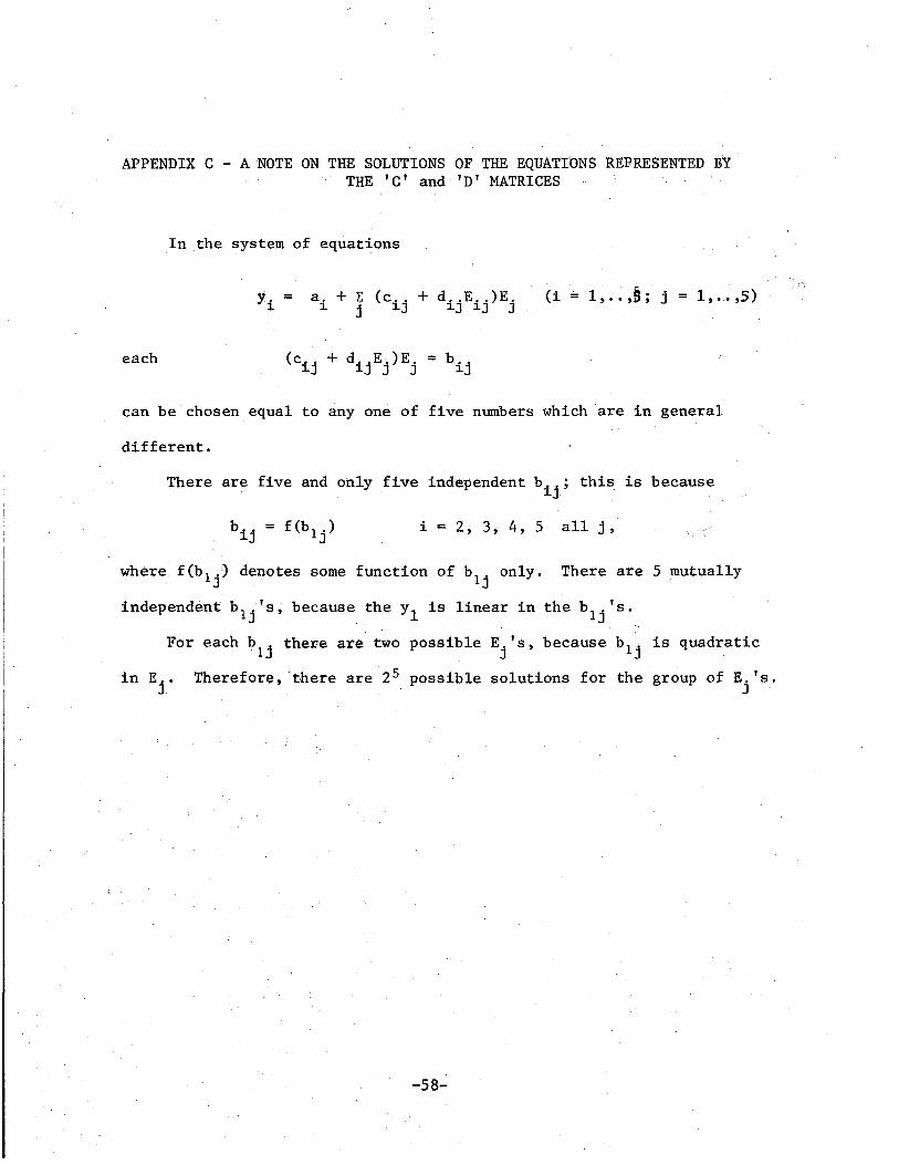
In the system of equations

a. + L: (c .. + d .. E .. )E. 1. j l.J l.J l.J J

(i "" 1' .. ,§; j = 1' .. ,5)

each

can be chosen equal to any one of five numbers which are in general

different.

There are five and only five independent b .. ; this is because l.J

i = 2, 3, 4, 5 all j ,

where f(b 1j) denotes some function of b1j only. There are 5 mutually

independent b1j's, because the y1

is linear in the b 1 . 's. . J

For each b1

j there are two possible Ej 's, because b 1 j is quadratic

Therefore, there are 25 possible solutions for the group of E.'s. J

-58-

APPENDIX D - COMPARISON BETWEEN THE DEFLECTIONS CAUSED IN A STRUCTURE REPRESENTING A HIGHWAY PAVEMENT BY A TRUCK WHEEL

WITH THOSE CAUSED IN THE SAME PAVEMENT BY THE DYNAFLECT AND iw A 12" PLATE

The effect of varying the moduli of the materials composing the layers

of the pavement was con$~de~ed.

Computations were performed for two structures:

(1) a 5 11 layer overlying a semi-infinite medium.

(2) a 25" layer overlying a semi-infinite medium.

The moduli of the materials composing the layer and the semi-infinite medium

were 200,000 and 10,000 psi respectively.

The loadings were represented as follows:

Truck Wheel - Two loads of 4,500 pounds exerting uniform

pressures of 100 psi, spaced 24" apart; the

deflection was calculated at the mid-point

of the line joining the load centers.

Dynaflect A total load of 1,000 pounds exerted on a

circle of radius 1.60"; the deflection was

calculated at a distance of 10" from the load.

12" Plate A uniform pressure of 100 psi exerted on a

plate 12" in diameter; the deflection was

calculated at the center of the plate.

For each layer, the effect was investigated of decreasing the modulus

of elasticity of the materials composing the layers by 5%. The decrease

was applied to each layer separately and then to both the layers simul-

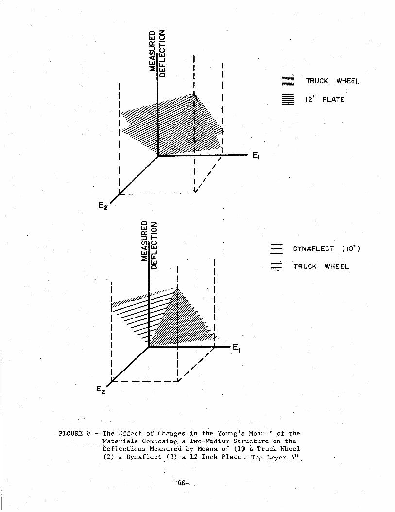
taneously. The results are plotted in Figure 8. From this figure the

-59·-

cz UJO o:::­::::>1-~fd I.LJ..J ::Elt

c ~· · TRUCK WHEEL

I I

'I I, _JI

------ 12" PLATE

DYNAFLECT ( to")

I I I I I I I I

~----+-----.,"--- E, /

/ /

/ -----..V

TRUCK WHEEL

FIGURE 8 - The Effect of Changes in the Young's Moduli of the Materials Composing a Two-Medium Structure on ·the Deflections Measured by Means of (101 a Truck Wheel (2) a Dynaflect. (3) a 12-Inch Plate . Top Layer 5"

-64)-

0 z w 0

§ t; <n w <( ..J w LL. :e w

0 z IJJ 0 0: I­;:) (.) <n LIJ <( ..J LIJ LL. 2 w

0

0

I / I / I//

----- __v

.

. . ·. TRUCK WHEEL

~- 12" PlATE

-· · •. TRUCK WHEEL

OYNAFLECT (10")

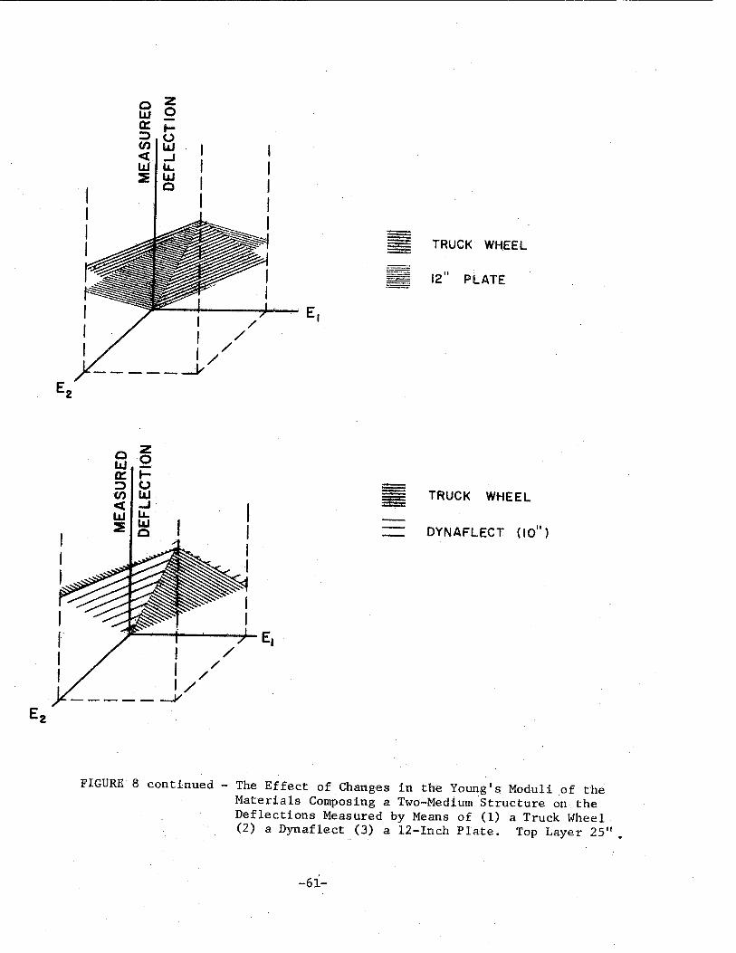
FIGURE 8 continued - The Effect of Changes in the Young's Moduli of the Materials Composing a Two-Medium 'structure on the Deflections Measured by Means of (1) a Truck Wheel (2) a Dynaflect (3) a 12-Inch Plate. Top Layer 25".

-61-

follow~ng appears:

(1) A change in the modulus of the top layer (E1) produces a greater

effect on all measurements if the top layer is thicker.

(2) The Dynaflect represents the behavior of the truck wheel more

closely than the measurements obtained from the 12" plate,

(3) The me·asurements of the deflections of the truck wheel are le&s

affected than those obtained from either the Dynaflect or the

12" plate by a change in E1 •

(4) The measurements of the deflections of the truck wheel are nicor.e

affected than those obtained from either the Dynaflect or the

12" plate by a change in E2 •

Conclusions (3) and (4) are not necessarily related.

-62-

APPENDIX E - LIST AND DESCRIPTIONS OF THE COMPUTER PROGRAMS ASSOCIATED WITH PART I OF THIS REPORT

Fortran Programs

The Fortran programs used in this work are intended for use with a

Watfor compiler but can be operated with only minor changes on an IBM/360/65

Fortran IV compiler.

Designation

WHC35

WHC36

Wang Programs

Description

Data checking program for the input to WHC 36. Supplies

a print-out of the input data in tabular form suitable

for rapid checking; requires less than a tenth of a

second for operation, and is an insurance against

wasted time when the longer running WHC 36 is operated.

Interpolates values of E. (j = 1 through 5), the Young's J

moduli of the materials composing the layers of a system

corresponding with a highway pavement. Requires about

twenty seconds to converge and contains some safety

features to prevent non-productive running.

(See Part 2 of this report for a description of the Wang computer)

Designation Description

6S4.xx where xx is a two digit parameter. This program has

been written in order to compute the elements of the

C and D matrices. As input to the program, a central

-63·-

Description

value of E is required. Values of Y are also needed;

they are computed by means of the Chevron program for

the central E and also for two neighboring E's which

are evenly spa~ed about the central E on a logarithmic

scale of E. The spacing is, therefore, denoted by a

factor, xx in the program designation. This factor

is to be punched in the Wang-program card in columns

2 and 3, and again in columns 18 and 19. Two columns

are thus available for the factor. If only a single

digit factor is required, punch the factor followed

by a decimal point, or a zero followed by the factor.

Details of operation: All input is in natural logarithms. The central E

value is placed in SRa; the Y's are placed in successively higher storage

registers, starting with the Y which corresponds with the lowest E. At

the end, the C element is read, and the D element from ~' if the Y's

are inserted in the reverse order from that specified above, the D elements

will be correct for use with WHC36, although the C's will not.

~64-

APPENDIX F - THE PLOTTING OF THE CROSS SECTION OF THE DEFLECTION BASIN IN A PAVEMENT WHICH IS SUBJECTED TO A POINT LOAD

It has been mentioned in the text that, for the case of a semi-

infinite homogeneous medium subjected to a point load perpendicular to

the free surface, the plot of (deflection x spacing) against spacing is

a horizontal straight line of ordinate equal to the product (deflection x

spacing). This is due to the relationship between deflection and spacing,

one of inverse proportionality (13). The plot obtained is indicated in

Figure, 9.

The systems which are of practical interest are not homogeneous

however. They consist of layers of materials which may be approximated

by isotropic elastic substances having a wide range of elastic moduli.

The layers may be composed of stiff and compliant materials, and may be

superposed in any order of stiffness.

Consider first the case of a layer of a compliant material overlying

a semi-infinite medium which is composed of a stiffer material. At spacings

which are large compared with the thickness of the layer, a horizontal

straight line is obtained; the ordinate of this line repre~ents a compliance

parameter of the material composing the underlying semi-infinite medium.*

Similarly, at spacings which are small compared with the thickness of the

layer, a horizontal straight line is obtained the ordinate of which represents

the same parameter relating to the layer. At spacings which are of the order

*This parameter is (1 ~ ~ 2 )/TIE per unit load (13), where E is the Young's modulus of the material and vis its Poisson's ratio.

-65-

~

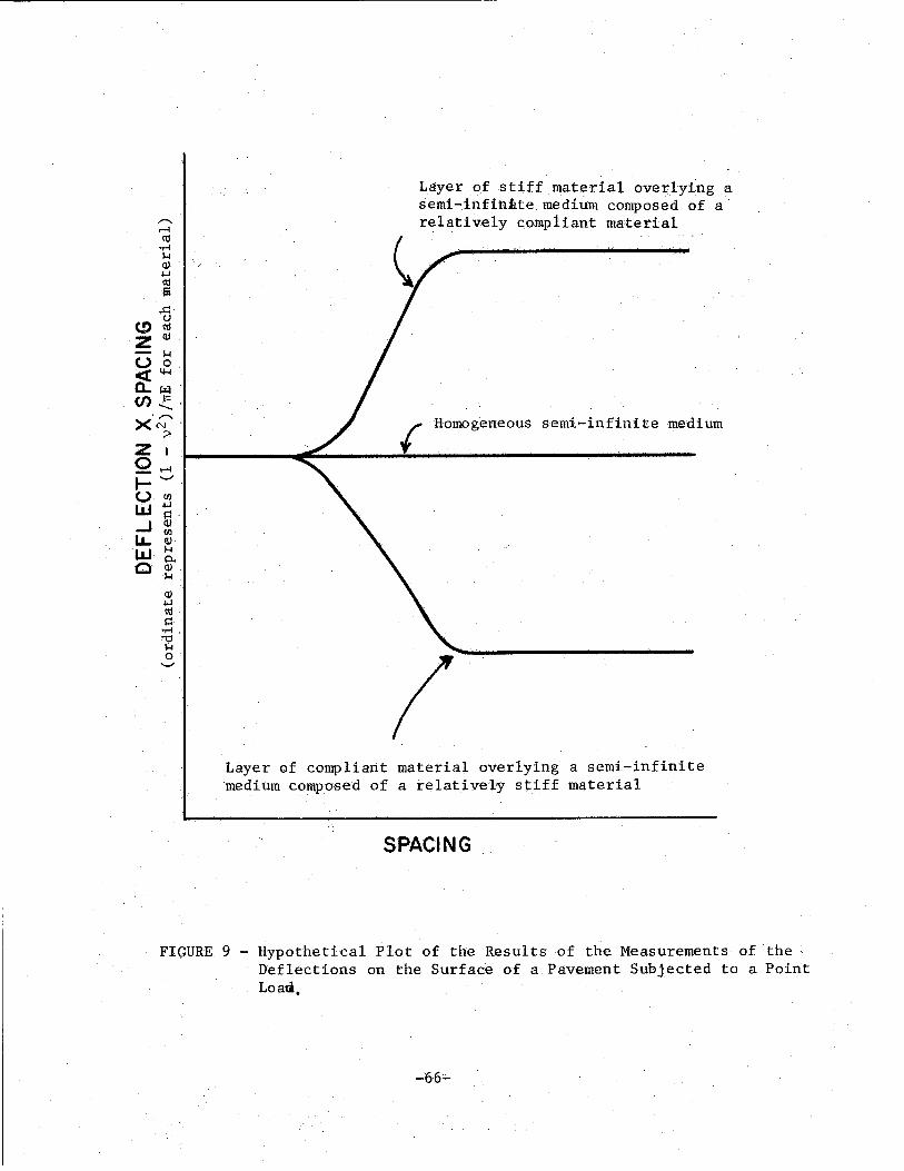
Layer of stiff material overlying a semi-infinite medium composed of a relatively compliant material

{ Homogeneous semi-infinite medium

I Layer of compliant material overlying a semi-infinite medium composed of a relatively stiff material

SPACING

FIGURE 9 - Hypothetical Plot of the Results of the Measurements of the · Deflections on the Surface of a Pavement Subjected to a Point Loali.

-66;;..

of the thickness of the layer a transition occurs; points, on the' curve,

including the transition, may be calculated by means of the Chevron

program (11, 12). The relationship is sketched in Figure 9.

If the overlying layer is composed of a stiffer material than the

semi-infinite medium, the form of the plot is reversed. At short spacings

the ordinate of the line represents the same parameter as before related

to the compliance of the layer. For large spacings, the ordinate represents

the parameter relating to the.underlying medium. The shape of the curve

is sketched in Figure 9; and points on the curve may be calculated if

required.

Although highway structures are not usually as simple as the ideal

system discussed here, some may be made to approximate such a structure.

Alternatively, this method may be applied to highway structures provided

the errors induced (usually by treating all the constructed layers as a

single one) are not important.

-67-

-----------------------------------------------------

LIST OF REFERENCES

1. Scrivner, F. H., Swift, Gilber,t and Mc:>ore_., W. M. "A New Resear~h Tool for Measuring Pavement Deflection," Highw-ay Res~arch. Record No. 129, 1966, pp. 1-11.

2. Scrivner~ F. H. and Moore, W. · M._ "Evaluation of the Stiffness -of _ Individual Layers in a Specially Designed Pavement Facility fro.m Surface Deflections," Research Report 32-8, Texas A&M University.

3. Scrivner, F. H. and Moore, W. M. "An Empirical Equation for Predicting Pavement Deflections," Texas Transportation Institute, College Station, Texas, October, 1968.

4. Cumming, D. A. and Gerrard, c. M. "Computation of Stresses in Pavements," Proceedings of the Second Conference ARRB, 2, Part 2, 729 (1964).

5. Timoshenko, S. P. "Theory of Elasticity," McGraw-Hill, 1951, Paragraph 123, Page 362.

6. Love, A. E. H. "The Mathematical Theory of Elasticity," New York. Dover. 1944, Paragraph 132, Page 186.

7. Filenko-Borodich, M., "Theory of Elasticity," New York. Dover. 1965. Paragraph 63. Page 280.

8. Swift, Gilbert. Private Communication.

9. Burmister, D. M. "The General Theory of Stresses and Displacements in Layered Soil Systems," J. Appl. Physics 16, (1945) , Part 1, pp. 89-94, Part 2, pp. 126-127, Part 3, pp. 296-302.

10. Kreysig, E., "Advanced Mathematics for Engineers," New York, Wiley, 1967. Page 485.

11. Michelow, J. "Analysis of Stresses and Displacements in anN-Layered Elastic System Under a Load Uniformly Distributed over a Circular Area," California Rese~rch Corporation, Richmond, California, September, 1963. · ·

12. Warren, H. and Dieckmann, W. L. "Numerical Computation of Stresses and Strains in a Multiple-Layered Asphalt Pavement System," California Research Corporation, Richmond, California, September, 1963.

13. Timoshenko, S. P. and Goodier, J. N. "Theory of Elasticity," New York, McGraw-Hill, 1951. Eqlfation 205, Page 365.

-68-

LIST OF REFERENCES (continued)

14. Biot, M. A. "Effect of Certairi Discontinuities on the Pressure Distribution in a Loaded Soil~" Eqysti:s 6, 367-375 (1935).

15. Pickett, G. "Stress Distributions in a Loaded Soil with Some Rigid Boundaries," Proceedings of 18th Annual Meeting of the Highway Research Board (1938), Part 2, pp. 35-48.

-69-