ANALYTICAL EXPRESSION OF THE MAGNETIC FIELD · PDF fileFIELD CREATED BY TILE PERMANENT MAGNETS...

Progress In Electromagnetics Research B, Vol. 13, 309–328, 2009

ANALYTICAL EXPRESSION OF THE MAGNETICFIELD CREATED BY TILE PERMANENT MAGNETSTANGENTIALLY MAGNETIZED AND RADIAL CUR-RENTS IN MASSIVE DISKS

R. Ravaud and G. Lemarquand

Laboratoire d’Acoustique de l’Universite du Maine, UMR CNRS 6613Avenue Olivier Messiaen, 72085 Le Mans, France

Abstract—In this paper, we present new expressions for calculatingthe magnetic field produced by either tile permanent magnetstangentially magnetized or by radial currents in massive disks. Theseexpressions are fully analytical, that is, we do not use any specialfunctions for calculating them. In addition, they are three-dimensionaland can be used for calculating the magnetic field for all regularpoints in space. The expressions commonly used for calculating themagnetic field produced by radial currents in massive disks are oftenbased on elliptic integrals or semi-analytical forms. We propose inthis paper an alternative analytical method that can also be used fortile permanent magnets. Indeed, by using the analogy between thecoulombian model and the amperian current model, radial currentsin massive disks can be represented by using the fictitious magneticpole densities that are located on two faces of a tile permanent magnettangentially magnetized. The two representations are equivalent andthus, the shape of magnetic field produced is the same for all pointsin space, with a smaller value in the case of it is produced by radialcurrents in massive disks. Such expressions can be used for realizingeasily parametric studies.

1. INTRODUCTION

The calculation of the magnetic field produced by radial currents inmassive disks has been studied by Babic, Akyel, Salon and Kincic [1, 2].Indeed, they obtained semi-analytical forms of the magnetic field

Corresponding author: G. Lemarquand ([email protected]).

310 Ravaud and Lemarquand

produced by radial current in massive disks by using the Biot-Savart Law. We propose in this paper to use another approachfor calculating the three components of the magnetic field producedby radial current in massive disks. Indeed, we use the Coulombianmodel instead of the Biot-Savart Law. By using the analogy betweenthe coulombian model and the amperian current model, we canshow that radial currents in massive disks can be represented astile permanent magnets whose polarization is perfectly tangential.In this case, the shape of the magnetic field produced by radialcurrent in massive disks is exactly the same as the one producedby a tile permanent magnet tangentially magnetized. However, itis noted that magnetic fields produced by radial currents are alwaysweaker than the ones produced by permanent magnets. Some previouscalculations of the magnetic field produced by tile or arc-shapedpermanent magnets were determined with the coulombian model [3–6]. In addition, other authors have proposed three-dimensional semi-analytical expressions for calculating the magnetic field produced bythick annular conductors [7–9]. More generally, such semi-analyticalexpressions can be employed for optimizing devices using cylindricalpermanent magnets [10–18]. The expressions obtained are oftenbased on one or two numerical integrations or elliptic integrals [19–21]. Consequently, some authors have proposed the use of toroidalfunctions for the computation of the external magnetic field producedby cylindrical permanent magnets [22–24].

The knowledge of the magnetic field produced by arc-shapedpermanent magnets is always interesting for the design of actuatorsor sensors [25–36].

This paper is composed in two parts.The first part deals with the analytical calculation of the magnetic

field produced by a tile permanent magnet tangentially magnetized.The three expressions of the magnetic components are determined byusing the coulombian model. Studying the magnetic field producedby tile permanent magnets tangentially magnetized can be interestingbecause such tile permanent magnets can be used for the designof magnetic couplings. We have represented in Fig 1 an exampleof structure using tile permanent magnets whose polarizations areperfectly tangential but with alternate polarizations. In addition,such tile permanent magnets can be used for the design of electricalmachines. Indeed, in a classical electrical machine, the radial fieldcreated by the stator constituted by an assembly of tile permanentmagnets whose polarizations are often radial can also be optimizedby adding tile permanent magnets tangentially magnetized in thisstructure. This way of assembling tile permanent magnets with several

Progress In Electromagnetics Research B, Vol. 13, 2009 311

H ( r, , z )

0 u ruz

u

Figure 1. Representation of an assembly of tile permanent magnetstangentially magnetized with alternate polarizations.

magnetizations allow one to optimize more easily the shape of the radialfield produced. Moreover, the magnetic field created by assemblies oftile permanent magnets radially and tangentially magnetized allow oneto obtain more intense magnetic fields inside such structures. This isinteresting for ironless structures with ferrofluid seals or for realizingmagnetic couplings. Furthermore, such tile permanent magnets areused for realizing Halbach structures. These kinds of structures arevery interesting because they allow us to create an uniform and intensefield inside a ring of tile permanent magnets. Eventually, we think thatsuch tile permanent magnets will be more and more used for realizingunconventional structures of stacked permanent magnets.

In the second part of this paper, we discuss the possibility ofusing the expressions of the magnetic field components created by atile permanent magnet tangentially magnetized for the case of massivedisks with radial currents. By comparing the coulombian model andthe amperian current model, we show that the two calculations arethe same. Such an analogy is interesting because the expressions ofthe magnetic field components produced by a tile permanent magnettangentially magnetized are fully analytical whereas the ones createdby radial currents in massive disks use elliptic integrals and one termmust be solved numerically [1]. Consequently, we show that it seemsto be possible to obtain a fully analytical expression of the magneticfield produced by radial currents in massive disks.


Ju

uz

ru0

2

1r2r1

z1

z2

Figure 2. Representation of the geometry considered. The tile innerradius is r1, the tile outer radius is r2, its angular width is θ2 − θ1. Itsmagnetic polarization is �J and its height is z2 − z1.

2. STUDY OF THE MAGNETIC FIELD PRODUCED BYA TILE PERMANENT MAGNET TANGENTIALLYMAGNETIZED

2.1. Notation and Geometry

The geometry considered and the related parameters are shown inFig. 2. The inner radius of the tile is r1, its outer radius is r2. Itsangular width equals θ2 − θ1 with θ2 > θ1. It height is z2 − z1 withz2 > z1. Its magnetic polarization is denoted �J and verifies for allpoints in tile tile permanent magnet the following equation:

�J = J�uθ (1)

This implies that the polarization of the tile permanent magnetis perfectly tangential. The magnetic field produced by such a tilepermanent magnet can be determined by using the coulombian model.Indeed, according to the Coulombian model, this tile permanentmagnet generates a magnetic field that can be deducted from itsmagnetic potential Φ(�r ) for all points in space. This magneticpotential is given by:

Φ(�r ) =1

4πμ0

⎛⎝∑

i

∫∫(Si)

�J · dSi∣∣∣�r − �̃r∣∣∣ +

∫∫∫(V )

−�∇ · �J∣∣∣�r − �̃r∣∣∣dV

⎞⎠ (2)

where Si represents one surface of the tile permanent magnet and V

its volume. In addition,∣∣∣�r − �̃r

∣∣∣ represents the distance between a


41n

n2

n

n

5

6

u

uz

ru

n3

0

n

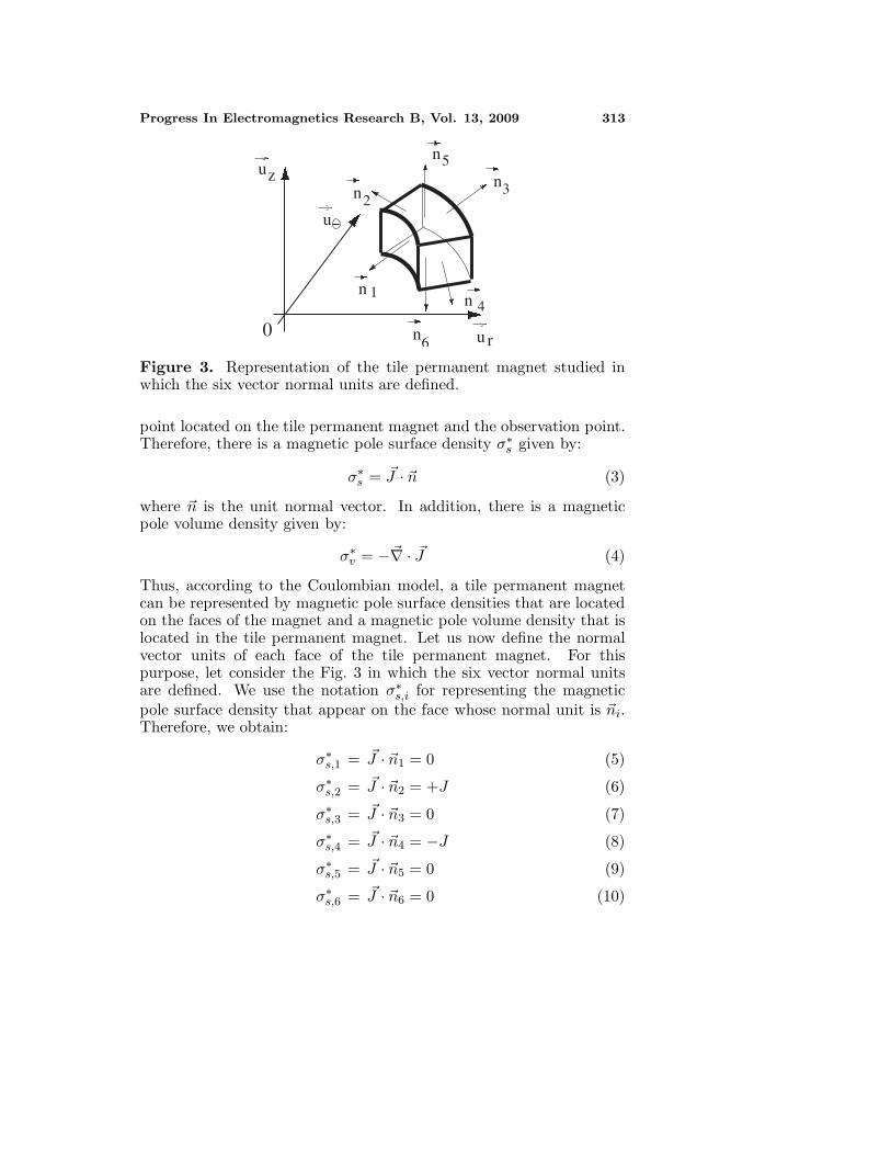
Figure 3. Representation of the tile permanent magnet studied inwhich the six vector normal units are defined.

point located on the tile permanent magnet and the observation point.Therefore, there is a magnetic pole surface density σ∗

s given by:

σ∗s = �J · �n (3)

where �n is the unit normal vector. In addition, there is a magneticpole volume density given by:

σ∗v = −�∇ · �J (4)

Thus, according to the Coulombian model, a tile permanent magnetcan be represented by magnetic pole surface densities that are locatedon the faces of the magnet and a magnetic pole volume density that islocated in the tile permanent magnet. Let us now define the normalvector units of each face of the tile permanent magnet. For thispurpose, let consider the Fig. 3 in which the six vector normal unitsare defined. We use the notation σ∗

s,i for representing the magneticpole surface density that appear on the face whose normal unit is �ni.Therefore, we obtain:

σ∗s,1 = �J · �n1 = 0 (5)

σ∗s,2 = �J · �n2 = +J (6)

σ∗s,3 = �J · �n3 = 0 (7)

σ∗s,4 = �J · �n4 = −J (8)

σ∗s,5 = �J · �n5 = 0 (9)

σ∗s,6 = �J · �n6 = 0 (10)


The magnetic pole volume density σ∗v can be determined by using the

definition of the divergence in cylindrical coordinates. We deduct that:

σ∗v = −�∇ · �J = 0 (11)

Consequently, only two magnetic pole surface densities appear on thetile permanent magnet tangentially magnetized. The first one −J islocated on the face whose angular abscissa equals θ1. The second one+J is located on the face whose angular abscissa equals θ2. We showa cross-section of the tile permanent magnet tangentially magnetizedwith its magnetic pole surface densities in the (R, θ) plane in Fig. 4.

J

u

ru

n

n

n

2

3

4

1n

1

2

r

r1

2

uz

Figure 4. Representation of the geometry considered. The tile innerradius is r1, the tile outer radius is r2, its angular width is θ2 − θ1. Itsmagnetic polarization is �J , its height is z2 − z1.

2.2. Three-dimensional Analytical Expression of theMagnetic Potentail Created by the Tile Permanent MagnetTangentially Magnetized

The reciprocal distance, in cylindrical coordinates, between the sourcepoint (r̃, θ̃, z̃) and the observation point (r, θ, z) is expressed as follows:

R(r̃, θ̃, z̃

)=

1∣∣∣�r − �̃r∣∣∣ =

1√r2 + r̃2 − 2rr̃ cos

(θ − θ̃

)+ (z − z̃)2

(12)

where �̃r represents the position vector of the source point and �r is theposition vector of the observation point. It is emphasized here thatthis reciprocal distance is not regular for all points in space. Thereis a discontinuity of this reciprocal distance when the magnetic field


is determined on the permanent magnet surfaces. Several approachescan be used for solving this problem. One method has been proposedby [3] with the use of the Lambda’s function. Another possibilityis to use the Cauchy principal value. By using the Gauss’ theorem,the magnetic field value can be easily verified when the observationpoint is placed on the permanent magnet surfaces. However, it can benoted that the magnetic field is rarely determined on the permanentmagnets but rather outside of the tile permanent magnets and alsoinside the permanent magnet for studying the demagnetizing field.All the analytical expressions presented in this paper can be used forstudying the three magnetic field components in the near-field.

Therefore, the magnetic potential Φ(r, θ, z) produced by a tilepermanent magnet tangentially magnetized is given by:

Φ(r, θ, z) =J

4πμ0

∫ r2

r1

∫ z2

z1

R (r̃, θ2, z̃) dr̃dz̃

− J

4πμ0

∫ r2

r1

∫ z2

z1

R (r̃, θ1, z̃) dr̃dz̃ (13)

After integrating according to r̃ and z̃, the magnetic potentialΦ(r, θ, z) can be expressed as follows:

Φ(r, θ, z) =J

4πμ0

2∑i=1

2∑j=1

2∑k=1

(−1)(i+j+k)φ(ai,j, bi,j , ck) (14)

where

φ(ai,j , bi,j , ck) =−zk −√

bi,j − a2i,j arctan

⎡⎣ ck√

bi,j − a2i,j

⎤⎦

+√

bi,j − a2i,j arctan

⎡⎢⎣ ai,jck√

bi,j − a2i,j

√bi,j + c2

k

⎤⎥⎦

−ck log[ai,j +

√bi,j+c2

k

]−ai,j log

[ck+

√bi,j+c2

k

](15)

and

ai,j = ri − r cos(θ − θj) (16)

bi,j = r2 + r2i − 2rri cos(θ − θj) (17)

ξk = z − zk (18)


Eq. (13) is in fact a special case in which the magnetic potentialhas a fully analytical form. It is emphasized here that this is rarelythe case for tile permanent magnets. Though the components of themagnetic field created by tile permanent magnets radially or axiallymagnetized can often be expressed in terms of elliptic integrals of thefirst, second and third kind, their magnetic scalar potential is oftenmore difficult to determine in a semi-analytical form. Moreover, it canbe easier to determine the magnetic field created by such tile permanentmagnets without using the vector or scalar potentials. We present inthe next section the expressions of the three components created bythe tile permanent magnet tangentially magnetized in fully analyticalexpressions.

2.3. Magnetic Field Produced by the Tile PermanentMagnet Tangentially Magnetized

A way of calculating the magnetic field produced by a tile permanentmagnet tangentially magnetized is to determine first the magneticpotential Φ(r, θ, z) for all points in space. We keep the notationξk (Eq. (18)) for the equations of the three magnetic componentsHr(r, θ, z), Hθ(r, θ, z) and Hz(r, θ, z).

2.4. Derivation of the Three Components

The magnetic field created by the tile permanent magnet tangentiallymagnetized can be deducted by calculating the following expression:

H = −�∇Φ(r, θ, z) (19)

and the three components are given respectively by:

Hr(r, θ, z) = −�∇Φ(r, θ, z) · �ur (20)

Hθ(r, θ, z) = −�∇Φ(r, θ, z) · �uθ (21)

Hz(r, θ, z) = −�∇Φ(r, θ, z) · �uz (22)

The three expressions obtained are also given in a fully analytical form.

2.5. Radial Component Hr(r, θ, z)

The radial component Hr(r, θ, z) is expressed as follows:

Hr(r, θ, z) =J

4πμ0

2∑i=1

2∑j=1

2∑k=1

(−1)(i+j+k)hr(i, j, k) (23)


where

hr(i, j, k) =

(−ei,j + cos (θ − θj)

2 fj

)√

fj(fj + bi,j)tanh−1

⎡⎣ ξk

√fj + bi,j√

fj

√bi,j + ξ2

k

⎤⎦

− cos (θ − θj)2 log

[ξk +

√bi,j + ξ2

k

](24)

withfj =

r

riei,j =

r

ri

(rri

(−1 + cos (θ − θj)

2))

(25)

We represent in Fig. 5 the radial component of the magnetic fieldproduced by a tile permanent magnet tangentially magnetized versusthe angle θ with the following parameters: r1 = 0.025 m, r2 = 0.028 m,r = 0.024 m, θ1 = − π

16 rad, θ2 = + π16 rad, z1 = 0 m, z2 = 0.003 m,

z = 0.0015 m, J = 1 T.

−0.4 −0.2 0 0.2 0.4Angle [rad]

−100000

−50000

0

50000

100000

Hr

[A/m

]

Figure 5. Representation of the radial component Hr versus the angletheta θ with the following parameters: r1 = 0.025 m, r2 = 0.028 m,r = 0.024 m, θ1 = − π

16 rad, θ2 = + π16 rad, z1 = 0 m, z2 = 0.003 m,

z = 0.0015 m, J = 1 T.

2.6. Azimuthal Component Hθ(r, θ, z)

The azimuthal component Hθ(r, θ, z) of the magnetic field produced bya tile permanent maget tangentially magnetized is expressed as follows:

Hθ(r, θ, z) =J

4πμ0

2∑i=1

2∑j=1

2∑k=1

(−1)(i+j+k)hθ(i, j, k) (26)


−0.4 −0.2 0 0.2 0.4Angle [rad]

−40000

−20000

0

20000

40000

Hth

eta

[A/m

]

Figure 6. Representation of the azimuthal component Hθ versusthe angle theta θ with the following parameters: r1 = 0.025 m,r2 = 0.028 m, r = 0.024 m, θ1 = − π

16 rad, θ2 = + π16 rad, z1 = 0m,

z2 = 0.003 m, z = 0.0015 m, J = 1T.

with

hθ = −yjcj + di,j√

cj (bi,j + cj)tanh−1

⎡⎣ ξk

√bi,j + cj√

cj

(bi,j + ξ2

k

)⎤⎦

+yj log[ξk +

√bi,j + ξ2

k

](27)

where

yj = sin(θ − θj) (28)

di,j = r2 − rri cos(θ − θj) (29)

cj = r2((cos (θ − θj))

2 − 1)

(30)

We represent in Fig. 6 the azimuthal component of the magnetic fieldproduced by a tile permanent magnet tangentially magnetized versusthe angle θ with the following parameters: r1 = 0.025 m, r2 = 0.028 m,r = 0.024 m, θ1 = − π

16 rad, θ2 = + π16 rad, z1 = 0 m, z2 = 0.003 m,

z = 0.0015 m, J = 1 T.


−0.4 −0.2 0 0.2 0.4Angle [rad]

−15000

−10000

−5000

0

5000

10000

15000

Hz

[A/m

]

Figure 7. Representation of the axial component Hθ versus the angletheta θ with the following parameters: r1 = 0.025 m, r2 = 0.028 m,r = 0.024 m, θ1 = − π

16 rad, θ2 = + π16 rad, z1 = 0 m, z2 = 0.003 m,

z = 0.001 m, J = 1 T.

2.7. Axial Component Hz(r, θ, z)

The axial component Hz(r, θ, z) of the magnetic field produced by atile permanent maget tangentially magnetized is expressed as follows:

Hz(r, θ, z) =J

4πμ0

2∑i=1

2∑j=1

2∑k=1

(−1)(i+j+k)hz(i, j, k) (31)

with

hz(i, j, k) = log[ri − r cos(θ − θj) +

√bi,j + ξ2

k

](32)

We represent in Fig. 7 the axial component of the magnetic fieldproduced by a tile permanent magnet tangentially magnetized versusthe angle θ with the following parameters: r1 = 0.025 m, r2 = 0.028 m,r = 0.024 m, θ1 = − π

16 rad, θ2 = + π16 rad, z1 = 0 m, z2 = 0.003 m,

z = 0.001 m, J = 1T.

2.8. Application of the Expressions Determined for theStudy of Ironless Structures Using Tile Permanent MagnetsTangentially Magnetized

All the expressions determined previously can be used easily for thestudy of the magnetic field produced by ironless structures usingassemblies of tile permanent magnets tangentially magnetized. Indeed,their computational cost is very low and they are very accurate. We


have represented the three-dimensional representations of the radialand azimuthal components of the magnetic field produced by anassembly of tile permanent magnets tangentially magnetized as shownin Figs. 8 and 9 respectively.

−0.02

0

0.02r m

−0.02

0

0.02

r [ m ]

−100

0

100Hr [kA/m]

0.02

0

0 02r [ m ]

Figure 8. Three-dimensional representation of the radial componentHr versus r in polar coordinates with the following parameters: r1 =0.025 m, r2 = 0.028 m, z1 = 0m, z2 = 0.003 m, z = 0.001 m, J = 1 Tand 8 tile permanent magnets are used.

−0.02

0

0.02r m

−0.02

0

0.02

r [ m ]

−500

50Htheta [ kA/ m]

0.02

0

0 02r [ m ]

Figure 9. Three-dimensional representation of the azimuthalcomponent Hθ versus r in polar coordinates with the followingparameters: r1 = 0.025 m, r2 = 0.028 m, z1 = 0 m, z2 = 0.003 m,z = 0.001 m, J = 1T and 8 tile permanent magnets are used.


3. MAGNETIC FIELD PRODUCED BY RADIALCURRENT IN MASSIVE DISKS WITH THECOULOMBIAN MODEL

We explain in this section how to calculate the magnetic field producedby radial currents in massive disks by using the coulombian model.Several authors have studied the magnetic field produced by suchstructures [1, 9]. In this paper, we study the particular case in whichboth surface current densities and a volume current density appear inmassive disks. Therefore, strictly speaking, our calculation does nottreat exactly the same configurations as [1] and [9] but the expressionsestablished in the first part of this paper can also be used for calculatingthe three components of the magnetic field created by radial currentsin massive disks. In fact, there is an analogy between our configurationstudied in the first part of this paper and the configurations studiedin [1] and [9]. We present in the next section this analogy.

3.1. Basic Equations

It is well known that the magnetic field produced by either a permanentmagnet or a current distribution can be determined by using either thescalar magnetic potential Φ(r, θ, z) or the vector magnetic potential�A(r, θ, z). We have shown in the first part that a tile permanent magnettangentially magnetized generates a scalar magnetic potential for allpoints in space. Let us now consider the magnetic vector potentialcreated by the tile permanent magnet tangentially magnetized studiedin the first part of this paper. This vector magnetic potential �A(r, θ, z)that is expressed as follows:

�A =μ0

4π

⎛⎝∫∫

(S)

�Jμ0

∧ dS∣∣∣�r − �r′∣∣∣ +

∫∫∫(V )

∇∧(

�Jμ0

)dV∣∣∣�r − �r′∣∣∣

⎞⎠ (33)

Therefore, we can say that there is a surface current density given by:

�k∗ =�J ∧ �n

μ0(34)

In addition, there is a volume current density given by:

�j∗ =∇∧ �J

μ0(35)


3.2. Application to a Tile Permanent Magnet TangentiallyMagnetized

Let us now apply the previous relations the configuration presented inFig. 2. According to the Amperian current model, a tile permanentmagnet tangentially magnetized can be represented by using (34)and (35). We find:

KS1 =J

μ0�uθ ∧ (−�ur) = − J

μ0�uz (36)

KS2 =J

μ0�uθ ∧ �uθ = 0 (37)

KS3 =J

μ0�uθ ∧ (�ur) = +

J

μ0�uz (38)

KS4 =J

μ0�uθ ∧ (−�uθ) = 0 (39)

KS5 =J

μ0�uθ ∧ (�uz) = +

J

μ0�ur (40)

KS6 =J

μ0�uθ ∧ (−�uz) = − J

μ0�ur (41)

In addition, the volume current density is expressed as follows:

�j∗ =∇μ0

∧ J�uθ =1μ0

1r

(∂(rJ)

∂r

)�uz =

J

r�uz (42)

We represent in Fig. 10 the surface current densities that are locatedon four faces of the tile permanent magnet and in Fig. 11 the surfacecurrent density that is located in the tile permanent magnet. Aninteresting point to say is that current on the face S1 and the currenton the face S3 are not the same because S3 > S1. This is why we cansay that a volume current density appears inside the tile permanentmagnet. This allows us to obtain a charge equilibrium of the magnet.Therefore, the three magnetic components peuvent also be determinedby using the following relation:

Hr(r, θ, z) =�∇μ0

∧ �A(r, θ, z).�ur (43)

Hθ(r, θ, z) =�∇μ0

∧ �A(r, θ, z).�uθ (44)

Hz(r, θ, z) =�∇μ0

∧ �A(r, θ, z).�uz (45)


r

uz

0

u

u

Figure 10. Representation of the surface current densities that appearon a tile permanent magne tangentially magnetized with the amperiancurrent model.

u

0 u r

uz

Figure 11. Representation of the volume current density thatappears inside a tile permanent magne tangentially magnetized withthe amperian current model.

In short, by assuming that there are radial currents in massive disksthat are characterized by both surface current densities k∗ and volumecurrent densities j∗, we can use directly the coulombian model byusing the transformations j∗ = �∇∧ �J

μ0and k∗ = �J∧�n

μ0. These two

transformations allow us to define the equivalent value of∣∣∣ �J ∣∣∣ that

correspond to a tile permanent magnet tangentially magnetized. Theinterest of such an approach lies in the fact that the expressions ofthe three magnetic components created by a tile permanent magnettangentially magnetized are fully analytical. Consequently, we can also


find in a fully analytical form the three magnetic components createdby radial currents in massive disks.

3.3. Illustration: Comparison with the Biot-Savart Law

The relations determined in the previous section can be compared withthe well-known Biot-Savart Law. For this purpose, let us consider theprevious configuration shown in Figs. 10 and 11 in which both a volumecurrent density �j∗ and four surface current densities kS1 , kS3 , kS5 andkS6 are considered. It is emphasized here that this configuration differsfrom the one studied in [1] and [9]. The magnetic field produced bysuch a current distribution is given by:

�H(�r) =14π

∫ r2

r1

∫ θ2

θ1

∫ z2

z1

�j∗dv ∧ (�r − �r′)∣∣∣�r − �r′∣∣∣3

+14π

∫ θ2

θ1

∫ z2

z1

�kS1dS1 ∧ (�r − �r′)∣∣∣�r − �r′∣∣∣3

+14π

∫ θ2

θ1

∫ z2

z1

�kS3dS3 ∧ (�r − �r′)∣∣∣�r − �r′∣∣∣3

+14π

∫ r2

r1

∫ θ2

θ1

�kS5dS5 ∧ (�r − �r′)∣∣∣�r − �r′∣∣∣3

+14π

∫ r2

r1

∫ θ2

θ1

�kS6dS6 ∧ (�r − �r′)∣∣∣�r − �r′∣∣∣3

(46)

For our numerical simulation, we take a surface current density∣∣∣�kSi

∣∣∣that equals 104 A/m2 and i is the surface i of the tile, r1 = 0.025 m,r2 = 0.028 m, z1 = 0 m, z2 = 0.003 m, θ1 = 0 rad, θ2 = π

8 rad,

and∣∣∣�j∗∣∣∣ that equals 104

r A/m3, θ = π7 rad, z = 0 m. We use the

magnetic induction field �B for the simulations and its calculation hasbeen performed by numerical means. We represent in Fig. 12 the radialcomponent of the magnetic induction field versus the radial observationpoint with the previous parameter values. Figure 12 confirms thevalidity of the coulombian model for calculating the magnetic fieldproduced by radial currents in massive disks.


0.026 0.028 0.03 0.032 0.034r m

0.6

0.4

0.2

0

0.2

0.4

0.6

BrmicroT

[ ]

[]

−

−

−

Figure 12. Representation of the radial component of the magneticinduction field �B determined with the coulombian model (thick line)and with the Biot-Savart Law (points). We take

∣∣∣�kSi

∣∣∣ = 104 A/m2

where i is the surface i of the tile, r1 = 0.025 m, r2 = 0.028 m, z1 = 0m,z2 = 0.003 m, θ1 = 0 rad, θ2 = π

8 rad,∣∣∣�j∗∣∣∣ = 104

r A/m3, θ = π7 rad,

z = 0m.

4. CONCLUSION

We have presented new expressions for calculating the magnetic fieldproduced by either a tile permanent magnet tangentially magnetized,or by radial currents in massive disks. All the expressions determinedin this paper are presented in a fully analytical form, that is,without any special functions as elliptic integrals. Consequently, suchexpressions have a very low computational cost and are accuratebecause all the expressions have been determined without anysimplifying assumptions. The analogy between the coulombian modeland the amperian current model allows us to calculate with the sameexpressions the magnetic field produced by tile permanent magnetswhose polarization is tangential or by radial currents in massive disks.

REFERENCES

1. Babic, S., C. Akyel, S. Salon, and S. Kincic, “New expressions forcalculating the magnetic field created by radial current in massivedisks,” IEEE Trans. Magn., Vol. 38, No. 2, 497–500, 2002.

2. Babic, S. and M. M. Gavrilovic, “New expression for calculatingmagnetic fields due to current-carrying solid conductors,” IEEETrans. Magn., Vol. 33, No. 5, 4134–4136, 1997.


3. Babic, S. and C. Akyel, “Improvement in the analytical calculationof the magnetic field produced by permanent magnet rings,”Progress In Electromagnetics Research C, Vol. 5, 71–82, 2008.

4. Ravaud, R., G. Lemarquand, V. Lemarquand, and C. Depollier,“Analytical calculation of the magnetic field created bypermanent-magnet rings,” IEEE Trans. Magn., Vol. 44, No. 8,1982–1989, 2008.

5. Ravaud, R., G. Lemarquand, V. Lemarquand, and C. Depollier,“The three exact components of the magnetic field createdby a radially magnetized tile permanent magnet,” Progress InElectromagnetics Research, PIER 88, 307–319, 2008.

6. Ravaud, R., G. Lemarquand, V. Lemarquand, and C. Depollier,“Discussion about the analytical calculation of the magnetic fieldcreated by permanent magnets,” Progress In ElectromagneticsResearch B, Vol. 11, 281–297, 2009.

7. Azzerboni, B. and E. Cardelli, “Magnetic field evaluation for diskconductors,” IEEE Trans. Magn., Vol. 29, No. 6, 2419–2421, 1993.

8. Azzerboni, B., E. Cardelli, M. Raugi, A. Tellini, and G. Tina,“Magnetic field evaluation for thick annular conductors,” IEEETrans. Magn., Vol. 29, No. 3, 2090–2094, 1993.

9. Azzerboni, B. and G. Saraceno, “Three-dimensional calculationof the magnetic field created by current-carrying massive disks,”IEEE Trans. Magn., Vol. 34, No. 5, 2601–2604, 1998.

10. Furlani, E. P., Permanent Magnet and Electromechanical Devices:Materials, Analysis and Applications, Academic Press, 2001.

11. Furlani, E. P., S. Reznik, and A. Kroll, “A three-dimensonal fieldsolution for radially polarized cylinders,” IEEE Trans. Magn.,Vol. 31, No. 1, 844–851, 1995.

12. Furlani, E. P. and M. Knewston, “A three-dimensional fieldsolution for permanent-magnet axial-field motors,” IEEE Trans.Magn., Vol. 33, No. 3, 2322–2325, 1997.

13. Furlani, E. P., “A two-dimensional analysis for the coupling ofmagnetic gears,” IEEE Trans. Magn., Vol. 33, No. 3, 2317–2321,1997.

14. Furlani, E. P., “Field analysis and optimization of ndfeb axial fieldpermanent magnet motors,” IEEE Trans. Magn., Vol. 33, No. 5,3883–3885, 1997.

15. Mayergoyz, D. and E. P. Furlani, “The computation ofmagnetic fields of permanent magnet cylinders used in theelectrophotographic process,” J. Appl. Phys., Vol. 73, No. 10,5440–5442, 1993.


16. Elies, P. and G. Lemarquand, “Analytical optimization of thetorque of a permanent-magnet coaxial synchronous coupling,”IEEE Trans. Magn., Vol. 34, No. 4, 2267–2273, 1998.

17. Lemarquand, V., J. F. Charpentier, and G. Lemarquand,“Nonsinusoidal torque of permanent-magnet couplings,” IEEETrans. Magn., Vol. 35, No. 5, 4200–4205, 1999.

18. Lang, M., “Fast calculation method for the forces and stiffnessesof permanent-magnet bearings,” 8th International Symposium onMagnetic Bearing, 533–537, 2002.

19. Babic, S. and C. Akyel, “An improvement in the calculation ofthe magetic field for an arbitrary geometry coil with rectangularcross section,” International Journal of Numerical Modelling:Electronic Networks, Devices and Fields, Vol. 18, 493–504,November 2005.

20. Babic, S., C. Akyel, and S. Salon, “New procedures for calculatingthe mutual inductance of the system: filamentary circular coil-massive circular solenoid,” IEEE Trans. Magn., Vol. 39, No. 3,1131–1134, 2003.

21. Babic, S., C. Akyel, and M. M. Gavrilovic, “Calculationimprovement of 3d linear magnetostatic field based on fictitiousmagnetic surface charge,” IEEE Trans. Magn., Vol. 36, No. 5,3125–3127, 2000.

22. Selvaggi, J. P., S. Salon, O. M. Kwon, M. V. K. Chari, andM. DeBortoli, “Computation of the external magnetic field, near-field or far-field from a circular cylindrical magnetic source usingtoroidal functions,” IEEE Trans. Magn., Vol. 43, No. 4, 1153–1156, 2007.

23. Selvaggi, J. P., S. Salon, O. M. Kwon, and M. V. K. Chari,“Computation of the three-dimensional magnetic field fromsolid permanent-magnet bipolar cylinders by employing toroidalharmonics,” IEEE Trans. Magn., Vol. 43, No. 10, 3833–3839, 2007.

24. Selvaggi, J. P., S. Salon, O. M. Kwon, and M. V. K. Chari,“Calculating the external magnetic field from permanent magnetsin permanent-magnet motors — An alternative method,” IEEETrans. Magn., Vol. 40, No. 5, 3278–3285, 2004.

25. Ravaud, R., G. Lemarquand, V. Lemarquand, and C. Depollier,“Ironless loudspeakers with ferrofluid seals,” Archives of Acous-tics, Vol. 33, No. 4, 3–10, 2008.

26. Wang, J., G. W. Jewell, and D. Howe, “Design optimisation andcomparison of permanent magnet machines topologies,” IEE Proc.Elect. Power Appl., Vol. 148, 456–464, 2001.


27. Yonnet, J. P., “Permanent magnet bearings and couplings,” IEEETrans. Magn., Vol. 17, No. 1, 1169–1173, 1981.

28. Zhu, Z., G. W. Jewell, and D. Howe, “Design considerationsfor permanent magnet polarised electromagnetically actuatedbrakes,” IEEE Trans. Magn., Vol. 31, No. 6, 3743–3745, 1995.

29. Abele, M., J. Jensen, and H. Rusinek, “Generation of uniformhigh fields with magnetized wedges,” IEEE Trans. Magn., Vol. 33,No. 5, 3874–3876, 1997.

30. Baran, W. and M. Knorr, “Synchronous couplings with sm co5magnets,” 2nd Int. Workshop on Rare-Earth Cobalt PermanentMagnets and Their Applications, 140–151, Dayton, Ohio, USA,1976.

31. Remy, M., G. Lemarquand, B. Castagnede, and G. Guyader,“Ironless and leakage free voice-coil motor made of bondedmagnets,” IEEE Trans. Magn., Vol. 44, No. 11, 2008.

32. Berkouk, M., V. Lemarquand, and G. Lemarquand, “Analyticalcalculation of ironless loudspeaker motors,” IEEE Trans. Magn.,Vol. 37, No. 2, 1011–1014, 2001.

33. Blache, C. and G. Lemarquand, “High magnetic field gradientsin flux confining permanent magnet structures,” Journal ofMagnetism and Magnetic Materials, Vol. 104, 1111–1112, 1992.

34. Blache, C. and G. Lemarquand, “New structures for lineardisplacement sensor with hight magnetic field gradient,” IEEETrans. Magn., Vol. 28, No. 5, 2196–2198, 1992.

35. Charpentier, J. F. and G. Lemarquand, “Optimization ofunconventional p.m. couplings,” IEEE Trans. Magn., Vol. 38,No. 2, 1093–1096, 2002.

36. Lemarquand, G., “Ironless loudspeakers,” IEEE Trans. Magn.,Vol. 43, No. 8, 3371–3374, 2007.

ANALYTICAL EXPRESSION OF THE MAGNETIC FIELD · PDF fileFIELD CREATED BY TILE PERMANENT MAGNETS...

Documents

Transcript of ANALYTICAL EXPRESSION OF THE MAGNETIC FIELD · PDF fileFIELD CREATED BY TILE PERMANENT MAGNETS...