ANALYTICAL AND NUMERICAL STUDIES OF

EFFECTIVE MEDIUM MIXING PROBLEMS IN ELECTROMAGNETICS

An Undergraduate Research Scholars Thesis

by

NICHOLAS N. MAI

Submitted to the Office of Honors and Undergraduate Research Texas A&M University

in partial fulfillment of the requirements for the designation as

UNDERGRADUATE RESEARCH SCHOLAR

Approved by Research Advisor: Dr. Gregory Huff

May 2013

Major: Electrical Engineering

1

TABLE OF CONTENTS

Page

TABLE OF CONTENTS………………………………………………………………………….1

ABSTRACT…………………..…………………………………………………………………...2

DEDICATION…………….………………………………………………………………………4

ACKNOWLEDGEMENTS……………………………………………………………………….5

NOMENCLATURE………………………………………………………………………...…….7

CHAPTER

I INTRODUCTION………………………………………………………………………...8

II THEORETICAL BACKGROUND……………………………………………………...11

Review of the theory of electromagnetics and dielectric materials……………...11 Classical mixing theory……………………………………………………..........13

III ANALYTICAL APPROACH…………………………………………………………...15

Single layered dielectric inclusions……………………………………………...15 Two layered dielectric inclusions………………………………………………..18 Field perturbation analysis………………………………………………………21

IV NUMERICAL SIMULATIONS…………………………………………………………23

COMSOL simulation setup and governing equations…………………………...26 CST Microwave Studio setup…………………………………………………....28 Results from COMSOL simulations……………………………………………..31

V CONCLUSIONS AND FUTURE WORK………………………………………………36

REFERENCES…………………………………………………………………………………..37

2

ABSTRACT

Analytical and Numerical Studies of Effective Medium Mixing Problems in Electromagnetics (May 2013)

Nicholas Mai Department of

Electrical & Computer Engineering Texas A&M University

Research Advisor: Dr. Gregory Huff

Department of Electrical & Computer Engineering

Electromagnetically Functionalized Colloidal Dispersions (EFCDs) have been utilized in several

applications in electromagnetics such as reconfigurable antennas. The colloidal dispersions vary

the electrical properties depending on the volume fraction relative to the background fluid. The

classical Maxwell-Garnett mixing formulas are an effective medium theory that provides a

capable framework for approximating the effective electromagnetic properties of these EFCD

mixtures. However, the theory only accounts for first-order interactions of the mixed inclusions

at lower volume fractions, so deviations from the theory occur at high volume fraction. Thus,

accurately modeling and predicting the effective permittivity of a mixture is still a problem to be

solved.

This thesis presents an analytical and numerical study of the effective properties for EFCDs. An

analysis in the quasi-static regime leads to the development of a new model that adds higher-

order interactions to the Maxwell Garnett theory. Additionally, finite-element simulations using

both COMSOL and Computer Simulation Technology Microwave Studio are performed to

compute the effective medium permittivity. Several particle distributions are analyzed using a

3

frequency dependent potential boundary condition to validate the analytical model as well as

study the effects of percolation at high volume fractions. These results will show that the

Maxwell-Garnett theory clearly breaks down at higher volume fractions.

4

DEDICATION

To my ALL of family and friends.

5

ACKNOWLEDGEMENTS

I would like to thank my research advisor, Dr. Gregory Huff, for his guidance and support

throughout the course of this most interesting project. My work would not have been possible if

not for the numerous resources he provided.

I am also deeply appreciative towards all of the members of the Huff Research Group. They

treated me as an equal despite all being much wiser and more experienced in the field of

electromagnetics.

In particular, I thank Franklin Drummond for the spending the countless hours (in particular,

Saturday March 23, 2013) helping me analyze and model this problem; without his assistance

and previous work, much of this thesis would not have been possible. I thank Michael Kelley for

providing much needed social support and mutual commiseration. I thank Kristopher Buchanan

for letting me use his own office space to do my research and work in the laboratory. I thank

Nicholas Brennan for allowing a second Nick in the lab and helping me finish computer related

tasks. I thank Joel D. Barrera for his assistance in handling the finer details of modeling RF

problems. I think David Rolando for being my office neighbor and listening to my many

mathematical ramblings.

I could not have finished this work without the support of my friends at this university, for they

never let me forget the importance of all work and no play.

6

Finally, my s would not have been possible if not for the sacrifices my family made to let me

come to this university.

7

NOMENCLATURE

AC Alternating Current

BCC Body-Centered Cubic

BSTO Barium Strontium Titanate

CST Computer Simulation Technology

CST-MWS Computer Simulation Technology – Microwave Studio

EFCD Electromagnetically Functionalized Colloidal Dispersions

EMT Effective Medium Theory

EQS Electro Quasi-Static

FCC Face-Centered Cubic

TE Transverse Electric

VSWR Voltage Standing-Wave Ratio

8

CHAPTER I

INTRODUCTION

The problem of characterizing a material’s electrical properties is extremely important to the

field of electromagnetics. The design of many high frequency components such as antennas and

transmission lines requires the knowledge of how electromagnetic fields affect and are affected

by a medium. For example, the attenuation and propagation constants in any transmission line

are directly related to the square root of the line’s dielectric permittivity [1].

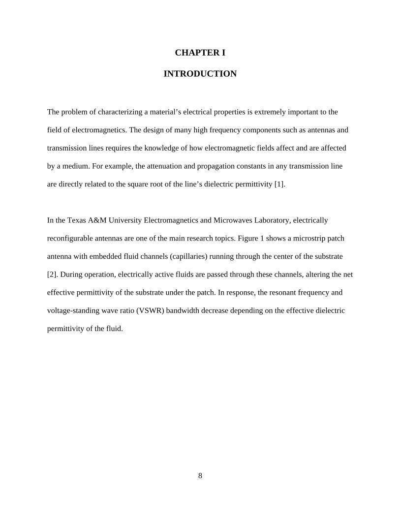
In the Texas A&M University Electromagnetics and Microwaves Laboratory, electrically

reconfigurable antennas are one of the main research topics. Figure 1 shows a microstrip patch

antenna with embedded fluid channels (capillaries) running through the center of the substrate

[2]. During operation, electrically active fluids are passed through these channels, altering the net

effective permittivity of the substrate under the patch. In response, the resonant frequency and

voltage-standing wave ratio (VSWR) bandwidth decrease depending on the effective dielectric

permittivity of the fluid.

9

Figure 1. Microfluidic reconfigurable patch antenna. Fluids passing through the channels beneath the patch antenna can alter the resonant frequency and VSWR bandwidth.

Figure 2 shows a cross-section of a typical fluid channel used in the laboratory. The fluid is

highly inhomogeneous and composed of electromagnetically functionalized colloidal dispersions

(EFCDs) mixed in with a background liquid. If there is a high contrast between the electrical

properties of these inclusions and the liquid, there is a change in the fluid’s net effective

electromagnetic properties according to a “mixing rule.” In general, the mixing rule is dependent

on the shape of the inclusion as well as the volume fraction relative to the background liquid [3].

Thus, when these fluids are used in the channels of patch antenna in Figure 1, reconfiguration

can be achieved by varying the inclusion types and volume fraction, which in turn vary the net

effective electromagnetic properties [2].

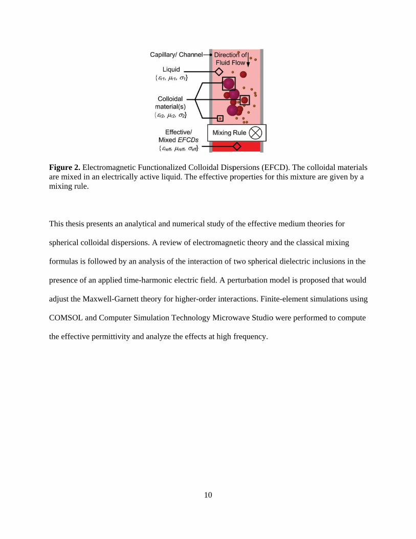
Figure 2are mixedmixing ru

This thes

spherical

formulas

presence

adjust the

COMSO

the effect

2. Electromagd in an electule.

sis presents a

l colloidal di

is followed

of an applie

e Maxwell-G

L and Comp

tive permitti

gnetic Functtrically activ

an analytical

ispersions. A

by an analy

ed time-harm

Garnett theor

puter Simula

ivity and ana

tionalized Coe liquid. The

l and numeri

A review of e

ysis of the int

monic electri

ry for higher

ation Techno

alyze the effe

10

olloidal Dispe effective p

ical study of

electromagn

teraction of

c field. A pe

r-order intera

ology Microw

fects at high

persions (EFproperties for

f the effectiv

etic theory a

two spherica

erturbation m

actions. Fini

wave Studio

frequency.

FCD). The cor this mixtur

ve medium th

and the class

al dielectric

model is prop

ite-element s

o were perfor

olloidal matere are given b

heories for

sical mixing

inclusions in

posed that w

simulations u

rmed to com

erials by a

n the

would

using

mpute

11

CHAPTER II

THEORETICAL BACKGROUND

This chapter lays the theoretical foundations for our analytical and numerical studies of effective

medium properties. The fundamental equations of electromagnetics are reviewed, and the

definition of dielectric materials and permittivity are explained in detail. Additionally, the

Maxwell-Garnett mixing rule is presented as the classical effective medium theory (EMT).

Review of the theory of electromagnetics and dielectric materials

In the field of electromagnetics engineering, the four most important partial differential

equations are the time-harmonic Maxwell’s equations [4]:

E j H

(1.1)

H j E J

(1.2)

·D

(1.3)

· 0B

(1.4)

Equations (1.1) and (1.2) are known as Ampere’s Law and Faraday’s Law, respectively; they

describe the coupling between the electric field E

and magnetic field H

fields in a given system.

Equations (1.3) and (1.4) are the Gauss’s laws for electric and magnetic fields; they state that the

point sources of electric fields are charges and that the point sources of magnetic fields do not

exist. Because these four equations govern electromagnetic fields, all of the problems in

electromagnetics can theoretically be solved by considering the equations with their proper

boundary conditions [4].

12

Equations (1.3) and (1.4) contain the field quantities D

and B

in place of the standard field

quantities because they describe the flux densities of the electric and magnetic fields. The

constitutive equations give the relation between the two sets of field quantities:

D E

(1.5)

B H

(1.6)

Here, the constants and represent the dielectric permittivity and magnetic permeability,

which are material properties that measure how a given medium responds to an electromagnetic

field. These two material quantities are often referred to by the relative quantities, r and r ,

whereby

0r (1.7)

0r (1.8)

and 0 and 0 are the properties for a vacuum.

Physically, the dielectric permittivity (or relative permittivity) is a measure of the polarizability

of a medium in the presence of an applied electric field. As an example, consider two parallel

plates with a medium in between such as in Figure 3. An electrical potential difference applied

across the two plates creates an electric field that passes through the sandwiched medium. The

field induces small dipole moments in the bound charge of the medium; altogether, the dipole

moments induce an electric field anti-parallel to the applied field. This “polarizing” effect is

what defines a dielectric medium.

13

Figure 3. Two parallel plates sandwiching a dielectric medium. When the potential difference V is applied across the plates, the internal bound and free charges align in the direction of the

applied field.

For dielectric materials, the constitutive relation, Equation (1.5), has an additional term:

D E P

(1.9)

where P

is the average polarization vector (or average dipole moment), which is parallel to the

direction of charge separation. In general, the relative dielectric permittivity of an anisotropic

material is a rank-2 tensor whose elements depend on the direction of the applied field. This can

become quite complicated, especially from a high-level, so the quantity “effective permittivity”

or “net permittivity” is often used to describe materials.

Classical mixing theory

The topic of this thesis is the calculation and characterization of the effective dielectric constant

eff for mixtures. Consider a simple model of anisotropy—isotropic particles dispersed in an

isotropic medium such as in Figure 2— and assume an electro quasi-static (EQS) regime, where

the time varying components such as charge and current are approximately stationary [5]. The

assumption requires that the size of the domain of interest is much smaller than one wavelength.

Then, Maxwell’s equations reduce to

14

0E

(1.10)

·D

(1.11)

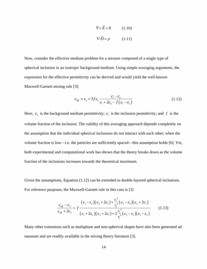
Now, consider the effective medium problem for a mixture composed of a single type of

spherical inclusion in an isotropic background medium. Using simple averaging arguments, the

expression for the effective permittivity can be derived and would yield the well-known

Maxwell-Garnett mixing rule [3]:

32

i eeff e e

i e i e

ff

(1.12)

Here, e is the background medium permittivity; i is the inclusion permittivity; and f is the

volume fraction of the inclusion. The validity of this averaging approach depends completely on

the assumption that the individual spherical inclusions do not interact with each other; when the

volume fraction is low—i.e. the particles are sufficiently spaced—this assumption holds [6]. Yet,

both experimental and computational work has shown that the theory breaks down as the volume

fraction of the inclusions increases towards the theoretical maximum.

Given the assumptions, Equation (1.12) can be extended to double-layered spherical inclusions.

For reference purposes, the Maxwell-Garnett rule in this case is [3]

32

1 2 1 2 1 131

32

1 2 1 2 1 131

22

2

2 2

2e eeff e

eff ee e

r

r

fr

r

(1.13)

Many other extensions such as multiphase and non-spherical shapes have also been generated ad

nauseam and are readily available in the mixing theory literature [3].

15

CHAPTER III

ANALYTICAL APPROACH

This chapter discusses the analytical approach to develop an effective permittivity formula that

accounts for the multi-particle interactions. In the laboratory applications, the standard dielectric

mixture are high dielectric Barium Strontium Titanate (BSTO) spherical inclusions dispersed in a

low dielectric silicone oil or electrically active fluid such as Flourinert FC-70. The oil or inert

fluid coats the outside of the spherical BSTO particles, forming a conductive shell. A conductive

(lossy) dielectric double-layer models the shell.

Single layered dielectric inclusions

Consider a layered dielectric sphere in the presence of an applied AC electric field such as in

Figure 4.

Figure 4. A layered dielectric sphere in the presence of a z -directed applied AC electric field. The outer layer is assumed to be lossy. As the electric field passes through the dielectric particle, a uniform internal field is induced, parallel to the direction of the primary field. Moreover, a net polarization is induced inside the layers.

16

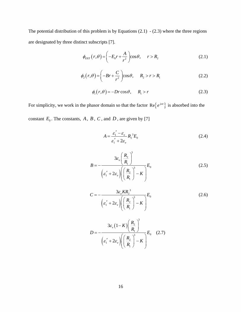
The potential distribution of this problem is by Equations (2.1) - (2.3) where the three regions

are designated by three distinct subscripts [7].

0 22, , cosEXT

Ar E r

rr R

(2.1)

22 2 1, , c s o C

r Br rr

R R

(2.2)

11 , cos , r Dr rR (2.3)

For simplicity, we work in the phasor domain so that the factor Re j te is absorbed into the

constant 0E . The constants, A , B , C , and D , are given by [7]

312 0

1 2e

e

A ER

(2.4)

3

2

103

21

1

3

2 e

e

R

ER

BR

KR

(2.5)

3

203

21

1

3

2 e

eKRC

RK

R

E

(2.6)

3

2

103

21

1

3 1

2 e

e

RK

R

RK

R

ED

(2.7)

17

Here, 1 is the effective permittivity of the double-layered particle, and K is the Clausius-

Mossotti factor. They are used instead of explicitly referring to the three different permittivities

to ensure that the mathematical expressions remain manageable [7]. Their values are given by

3

2 1 2

1 1 21 2 3

2 1 2

1 1 2

22

22

RR

RR

(2.8)

1

1 2e

e

K

(2.9)

Additionally, the permittivities can be complex valued, 0

n

nn r j

. From Equations (2.1)

through (2.3), the corresponding electric field is simply computed as ,E r , where the

gradient is taken in cylindrical coordinates.

0 30 3

2 ˆˆ ˆcos cos s, sin inEXT

A Ar E

rE r E r

r

(2.10)

32 3ˆˆ

2ˆcos c, s o sinin s

C Cr B

rE r B r

r

(2.11)

1 ˆcos, sinE D rr D

(2.12)

The electric field expressions above are written in a form that separates the 3

1

r dependency in

the various terms. Examining the expression for the external field, we can see that the field is

given by the superposition of the applied field and the perturbation in the presence of the layered

dielectric sphere. Mathematically, we can then write

, , ,EXT APP PERTURBED rE Er rE

(2.13)

18

As one gets far enough away from the layered sphere, the field appears uniform. In the rest of

this thesis, an approximation is made that when 210r R , the field can be considered uniform

because the perturbing field will have been reduced by 310 , or -3 dB.

Two layered dielectric inclusions

Now consider a system of two layered dielectric particles, spaced a distance dR from each other

(see Figure 5).

Figure 5. Two layered dielectric spheres separated by a distance dR .

Just as before, the applied electric field induces a polarization inside each particle. Physically,

this causes the free charge from the lossy surface to reorient along the edges, such as in Figure 6.

As dR gets smaller, the particles become closer, which models an increased volume fraction.

This charge separation then induces a second order interaction between the two particles,

modeled as an induced polarization anti-parallel to the direction of the applied field.

19

Figure 6. Induced polarization on both spheres. A charge separation is formed on the surface and distributes itself in the direction of the induced polarization.

Figure 7. Polarization induced by the charge separation on surface of the spheres.

Mathematically, suppose that he first particle is located at the center of a cylindrical coordinate

system; the second particle would then be a vertical displacement dR away. Figure 8 displays the

geometrical setup. Then, the relation between the primed and unprimed coordinate systems is

given by

2 2 2 cosd dr r R rR (2.14)

20

1

2 2

2 cos

2 2 coscos d

d d

R r

r R rR

(2.15)

The external potential generated by shifted dielectric sphere is

2 20 2 2

, 2 cos cos2 cosd

d dE dXT

Ar E r R rR

r R rR

(2.16)

Now, recalling the trigonometric identity relating a shifted cosine term, the term cos becomes

1

2 2 2 2

2 cos 2 coscos

2cos cos

2 cos 2 2 cosd d

d d d d

R r R r

r R rR r R rR

(2.17)

To evaluate the external field, one can either evaluate the gradient on the shifted external

potential or substitute the coordinate transformations. The final expression for the external field

of the shifted dielectric is a complex expression in terms of the original spherical coordinates.

1

e 2 ,

r

1

2 ,

dR

r

jt

EEz

e0ˆ Re{

}

Figure 8. Geometry of the shifted second particle.

21

If the distance between these particles is greater than the limit defined in the previous subsection,

the total external electric field appears uniform, and the interaction between the particles is

negligible.

Field perturbation analysis

Using the two-particle framework developed in the previous subsection, consider the problem of

the two dielectric spheres as they approach one another. This physically occurs in the fluid

mixture as the volume fraction approaches the percolation threshold, and the interactions

between each of the particles are no longer negligible. Using the radial limit defined in the prior

subsection, let the electric field outside of a given particle be given by

, 10, , 10

, , 10, , 10,

EXTEXT UNIFORM pp

INTEXT INTEXTEXT pp

Er

E

E r rr r rE

r r rr r rE

(2.18)

where the field is now divided into two regions, inside and outside of the radial limit.

If the two dielectric spheres are far enough apart, the field seen at the center point between the

particles is approximately just the uniformly applied field. Now consider the situation when the

two particles are close enough such that the center point between the two fields is inside of the

radial limit of both particles. In this overlapping region, the electric field is a positive

perturbation on the normal field inside the radial limit. This perturbed interaction is a model for

the two-particle interaction as the volume fraction of the spherical inclusions increases to and

past the percolation threshold.

22

With some physical intuition, this perturbation can be modeled as the inclusion of a high

dielectric prolate spheroid between the particles. As the volume fraction increases, there is

deviation from the Maxwell-Garnett theory, and the measured effective permittivity is greater

than the predicted value. Currently, this model is not completely resolved. However, the

technique would be to analyze the perturbation back-calculate what the dimensions and

permittivity of the induced prolate spheroid should be that would resemble the deviation from

Maxwell-Garnett. Then, a new effective medium formula can be derived using a standard

multiphase mixture analysis.

23

CHAPTER IV

NUMERICAL SIMULATIONS

This chapter discusses the finite-element simulations performed to compute the effective

permittivity of various particle geometries and compare them with the classical Maxwell-Garnett

effective medium theories. Two different finite-element programs were used: COMSOL

Multiphysics and Computer Simulation Technology - Microwave Studio (CST-MWS). In

COMSOL, the setup consisted of modeling a periodic unit-cell and applying a bias voltage

between two the two faces; the volume-average electric field and electric displacement fields

were computed to solve for the effective permittivity. This method is adopted from Lee et al. [8]

During the analysis, COMSOL failed at lower-frequencies and yielded some numerical

inaccuracies, so CST-MWS was chosen as a secondary benchmark. Following the material

measurements technique used in the laboratory, transverse electric (TE) plane-wave incidence on

the periodic unit cell was simulated using a Floquet analysis, and the effective permittivity was

extracted from the computed de-embedded 21S parameter.

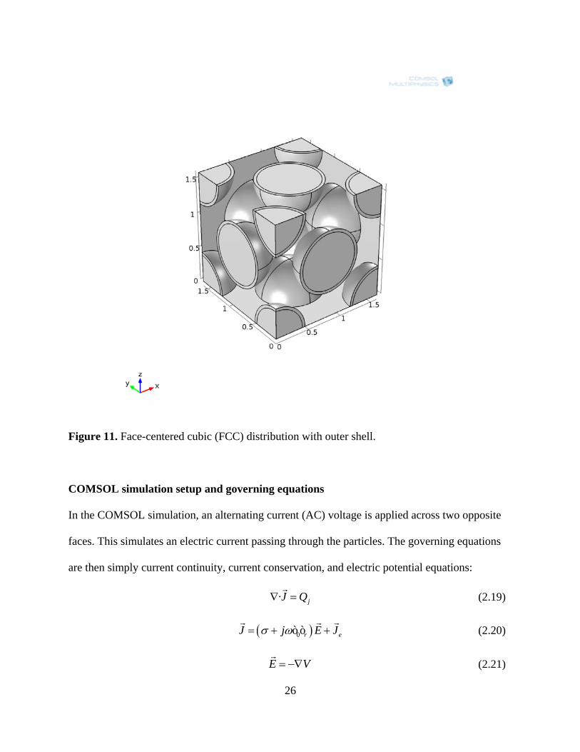
To model a large distribution of colloidal dispersions, a periodic unit cell was analyzed for

various known crystal lattice configurations. These consist of the simple-cubic, body-centered

cubic, and face-centered cubic lattices. The domain is then the particles aligned according to one

of the distributions and a background fluid. Periodic boundary conditions applied on four

adjacent faces simulate an infinite extension in two dimensions while an applied AC voltage or

incident wave excites the structure. Figures 8-10 show the various distributions as they were in

COMSOL. The CST-MWS model was geometrically the same.

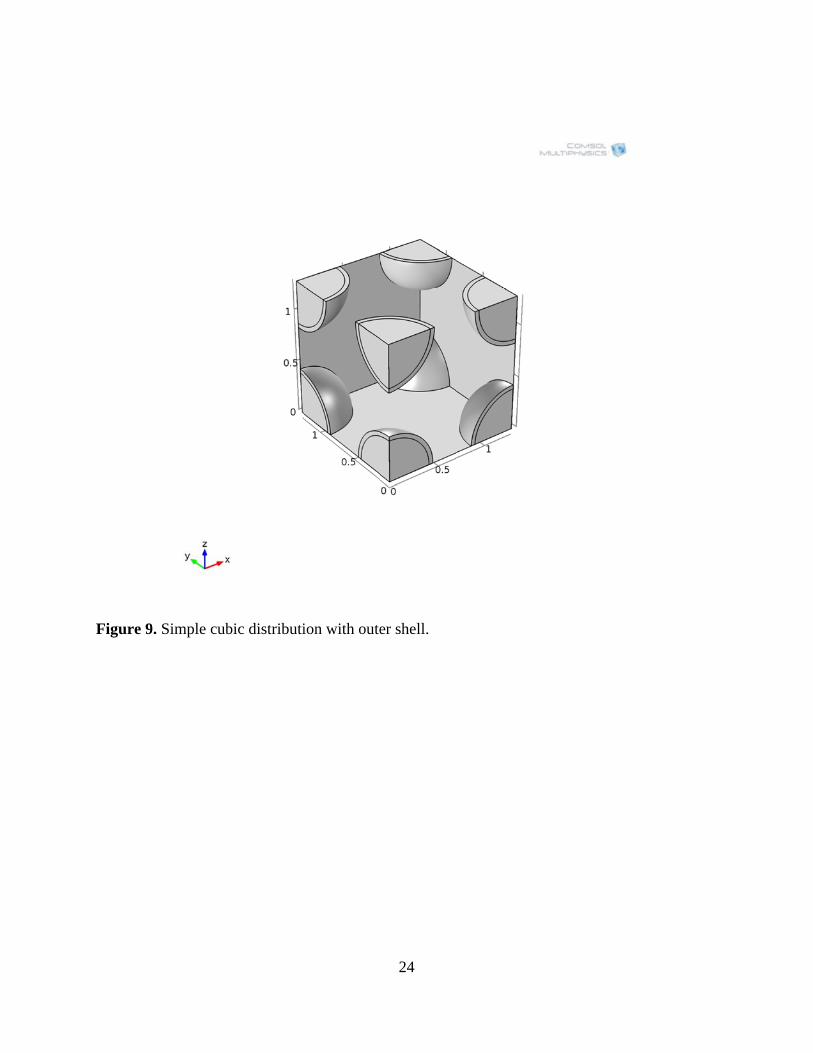
Figure 9

9. Simple cubbic distributiion with oute

24

er shell.

Figure 1

0. Body-cenntered cubic (BCC) distr

25

ibution withh outer shell.

26

Figure 11. Face-centered cubic (FCC) distribution with outer shell.

COMSOL simulation setup and governing equations

In the COMSOL simulation, an alternating current (AC) voltage is applied across two opposite

faces. This simulates an electric current passing through the particles. The governing equations

are then simply current continuity, current conservation, and electric potential equations:

· jJ Q

(2.19)

0 r eJ j E J

ò ò (2.20)

E V

(2.21)

27

The effective permittivity of a single unit cell can be extracted from the basic constitutive

relation Equation (1.5). In order for this method to be valid, all of the materials are assumed to be

linear and isotropic. In matrix form, the constitutive relation is

x xx xy xz x

y yx yy yz y

z zx zy zz z

D E

D E

D E

(2.22)

The assumption of isotropy and linearity leads to a symmetric permittivity matrix. Furthermore,

since the field is applied in a single direction, the exciting vector field E

can be approximated

by

0

0

xE

E

(2.23)

This simplifies Equation (2.22) yielding

0

0

x xx x

y yx

z zx

D E

D

D

(2.24)

Equation (2.24) is dependent on the location within the discretized unit cell. Taking a volumetric

average of the four field quantities in Equation (2.24) extracts the volumetric average

permittivity components.

0

0

x xx x

y yx

zxz

D E

D

D

(2.25)

Since the particle distribution consists of uniformly shaped spherical inclusions, the total

effective permittivity has only one non-zero component, xx . The analysis above assumes an

excitation in the x direction. A similar setup with excitations in the y and z directions results

28

in the other diagonal components of the permittivity matrix, yy and zz . Finally, by symmetry

arguments,

yyx zzx (2.26)

up to numerical accuracy of the discretization.

CST Microwave Studio setup

In contrast to the volumetric averaging technique in COMSOL, the effective property simulation

with CST-MWS is based on the material measurements technique used in the laboratory [9]. An

unknown material is placed between two known materials. A plane-wave is excited at the first

boundary, which transmits and reflects through the material. Floquet ports with only the TE00

modes model the incident plane wave. The frequency domain solver is used. CST-MWS can

extract the scattering parameters of the system. The remaining task is to extract the material

permittivity from the parameters.

Computing Material Properties from Scattering Parameters

Consider a three-part scattering problem modeled as a two-port transmission line network, such

as in Figure 12. An electromagnetic plane wave incident to the material under test (MUT)

reflects and transmits through both boundaries of the medium. The two-port scattering

parameters capture the physics of the bouncing reflections and transmissions on both interfaces.

The reflection coefficient between the first outer-MUT interfaces is

29

1

11

1

1

s

s

r r

r rs

s r r

r r

Z Z

Z Z

Z Z

Z Z

(2.27)

where sZ and Z are the sample and boundary impedances, respectively, normalized to the

impedance of air, 0 .

rs

r

Z

(2.28)

Figure 12. Two-port network model to measure material properties.

1

1

r

r

Z

(2.29)

In general, the material properties and are complex quantities. For the purposes of this

analysis, the outer material is assumed to be lossless. The reflection coefficient at the second

MUT-outer boundary is 12 . The transmission coefficient through the MUT is

30

0 0

2r r

r rs

j dj dj dT e e e

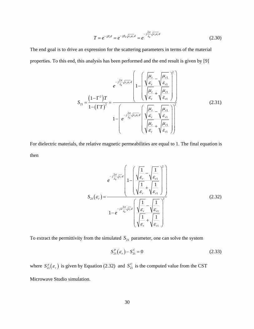
(2.30)

The end goal is to drive an expression for the scattering parameters in terms of the material

properties. To this end, this analysis has been performed and the end result is given by [9]

0

0

2

1

1

1

21

21 2 2

2

1

1

1

1

2

1

1

1

1r r

r r

r r

j dr r

r r

r r

r r

j dr r

r r

r r

T

e

TS

e

(2.31)

For dielectric materials, the relative magnetic permeabilities are equal to 1. The final equation is

then

0

0

2

1

1

21 2

21

1

2

2

1 1

1 1

1

1

1

11 1

r

r

j dr r

r r

r

j dr r

r r

e

S

e

(2.32)

To extract the permittivity from the simulated 21S parameter, one can solve the system

21 21 0rP CS S (2.33)

where 21 rpS is given by Equation (2.32) and 21

CS is the computed value from the CST

Microwave Studio simulation.

Results f

In both c

distributi

double la

be a silic

was inclu

frequency

In all of t

they all r

Figure 1

from COMS

onfiguration

ions. The inc

ayer had a lo

one oil with

uded for the

y were perfo

the COMSO

resemble Fig

3. Potential

SOL simula

ns, various si

clusions con

ossy conduct

h a dielectric

silicone oil.

ormed.

OL cases, the

gure 13, vary

distribution

ations

imulations w

sisted of eith

tivity. In both

constant of

Parametric

e field solutio

ying only slig

across a BC

31

were run for

her a single o

h simulation

2.1. In the C

sweeps over

ons were plo

ghtly depend

CC particle d

the BCC, FC

or double lay

ns, the backg

CST-MWS c

r particle rad

otted over th

ding on the c

distribution.

CC, and sing

yer dielectri

ground fluid

case, a small

dii, particle p

he special dom

chosen partic

gle particle

c, where the

was chosen

conductive

permittivity,

main. In gen

cle distributi

e

to

loss

and

neral,

ion.

32

Figure 14. BCC COMSOL Computed Permittivity at 3GHz and 500r .

33

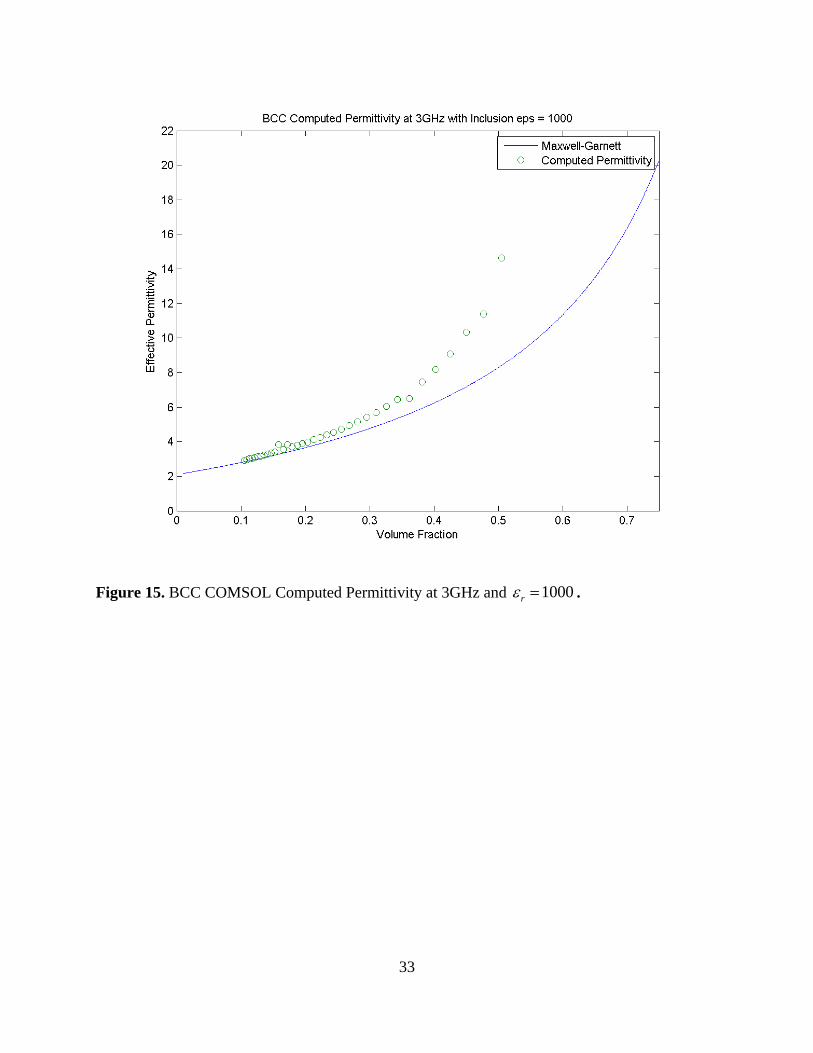
Figure 15. BCC COMSOL Computed Permittivity at 3GHz and 1000r .

34

Figure 16. FCC COMSOL Computed Permittivity at 3GHz and 500r .

35

Figure 17. FCC COMSOL Computed Permittivity at 3GHz and 1000r .

Figures 14-17 above show the computed results from the COMSOL simulations at 3GHz for two

different particle permittivities. Clearly, a deviation from Maxwell-Garnett is seen as the volume

fraction increases above 30%.

Currently, the simulation results from CST-MWS are still being analyzed, so they are not

available.

36

CHAPTER V

CONCLUSIONS AND FUTURE WORK

The analytical model presented in this thesis provides insight into modeling the interactions

between multiple particles in a mixed medium. Modeling of the prolate inclusions will modify

the standard Maxwell-Garnett formulas and likely account for the increase in effective

permittivity seen by the numerical simulations. COMSOL Multiphysics proved to be problematic

at handling low-frequency calculations, but at 3GHz, the results clearly indicate a deviation from

Maxwell-Garnett.

Future work includes finishing the perturbation analysis on the two-particle inclusion to compute

a new effective medium formula. Additionally, further investigation into how COMSOL

numerically solve the partial differential equations will be performed to verify the validity of the

software package. Further, the analysis on the CST-MWS studio will be completed to examine

the computed effective permittivity with this method. Laboratory analysis using the material

measurements system will be undertaken to serve as a final comparison between the classical

theory, new model, and numerical results.

37

REFERENCES

[1] David M. Pozar, Microwave Engineering, 4th ed. Hoboken, New Jersey: John Wiley &

Sons, 2012.

[2] Sean Goldberger et al., "Frequency Reconfiguration of a Small Array Enabled by Functionalized Dispersions of Colloidal Material," in 23rd Annual Conference on Small Satelites, Logan, UT, 2009.

[3] Ari Sihvola, Electromagnetic Mixing Formulas, 1st ed. London, United Kingdom: The Institution of Electrical Engineers, 1999.

[4] Julias A. Stratton, Electromagnetic Theory. Hoboken, New Jersey: John Wiley & Sons, 2007.

[5] Roger F. Harrington, Time-Harmonic Electromagnetic Fields. Hoboken, New Jersey: John Wiley & Sons, 2001.

[6] A. Alexopoulos, "Effective-medium theory of surfaces and metasurfaces containing two-dimensional binary inclusions," Physical Review E, vol. 81, no. 046607, pp. 1-12, April 2010.

[7] Thomas B. Jones, Electromechanics of Particles, 1st ed. Cambridge, United Kingdom: Cambridge University Press, 1995.

[8] J., J. Lee, J. G. Boyd, and D. C. Lagoudas, "Effective Properties of Three-Phase Electro-Magneto-Elastic Composites," International Journal of Engineering Science, vol. 43, pp. 790-825, 2005.

[9] A. M. Nicholson and G. F. Ross, "Measurement of the Intrinsic Properties of Materials by Time-Domain Techniques," IEEE Transactions on Instrumentation and Measurement, vol. 19, no. 4, pp. 377-382, November 1970.

[10] Franklin Drummond, "Finite Element Studies of Colloidal Mixtures Influenced by Electric Fields," Texas A&M University, August 2011.