Analytic and simulation methods in computer network design*

by LEONARD KLEINROCK

University of California Los Angeles, California

INTRODUCTION

The Seventies are here and so are computer networks! The time sharing industry dominated the Sixties and it appears that computer networks will play a similar role in the Seventies. The need has now arisen for many of these time-shared systems to share each others' resources by coupling them together over a communica­tion network thereby creating a computer network. The mini-computer will serve an important role here as the sophisticated terminal as well as, perhaps, the message switching computer in our networks.

I t is fair to say that the computer industry (as is true of most other large industries in their early de­velopment) has been guilty of "leaping before looking"; on the other hand "losses due to hesitation" are not especially prevalent in this industry. In any case, it is clear that much is to be gained by an appropriate mathematical analysis of performance and cost measures for these large systems, and that these analyses should most profitably be undertaken before major design commitments are made. This paper attempts to move in the direction of providing some tools for and insight into the design of computer networks through mathe­matical modeling, analysis and simulation. Frank et al.,4 describe tools for obtaining low cost networks by choosing among topologies using computationally efficient methods from network flow theory; our ap­proach complements theirs in that we look for closed analytic expressions where possible. Our intent is to provide understanding of the behavior and trade-offs available in some computer network situations thus creating a qualitative tool for choosing design options and not a numerical tool for choosing precise design parameters.

* This work was supported by the Advanced Research Projects Agency of the Department of Defense (DAHC15-69-C-0285).

THE ARPA EXPERIMENTAL COMPUTER NETWORK—AN EXAMPLE

The particular network which we shall use for pur­poses of example (and with which we are most familiar) is the Defense Department's Advanced Research Projects Agency (ARPA) experimental computer network.2 The concepts basic to this network were clearly stated in Reference 11 by L. Roberts of the Advanced Research Projects Agency, who originally conceived this system. Reference 6, which appears in these proceedings, provides a description of the his­torical development as well as the structural organiza­tion and implementation of the ARPA network. We choose to review some of that description below in order to provide the reader with the motivation and understanding necessary for maintaining a certain degree of self containment in this paper.

As might be expected, the design specifications and configuration of the ARPA network have changed many times since its inception in 1967. In June, 1969, this author published a paper8 in which a particular network configuration was described and for which certain analytical models were constructed and studied. That network consisted of nineteen nodes in the con­tinental United States. Since then this number has changed and the identity of the nodes has changed and the topology has changed, and so on. The paper by Frank et al.,4 published in these proceedings, describes the behavior and topological design of one of these newer versions. However, in order to be consistent with our earlier results, and since the ARPA example is intended as an illustration of an approach rather than a precise design computation, we choose to con­tinue to study and therefore to describe the original nineteen node network in this paper.

The network provides store-and-forward communica­tion paths between the set of nineteen computer re-

569

570 Spring Joint Computer Conference, 1970

Figure 1—Configuration of the ARPA network in Spring 1969

search centers. The computers located at the various nodes are drawn from a variety of manufacturers and are highly incompatible both in hardware and soft­ware ; this in fact presents the challenge of the network experiment, namely, to provide effective communica­tion among and utilization of this collection of incom­patible machines. The purpose is fundamentally for resource sharing where the resources themselves are highly specialized and take the form of unique hard­ware, programs, data bases, and human talent. For example, Stanford Research Institute will serve the function of network librarian as well as provide an efficient text editing system; the University of Utah provides efficient algorithms for the manipulation of figures and for picture processing; the University of Illinois will provide through its ILLIAC IV the power of its fantastic parallel processing capability; UCLA will serve as network measurement center and also provide mathematical models and simulation capability for network and time-shared system studies.

The example set of nineteen nodes is shown in Figure 1. The traffic matrix which describes the message flow required between various pairs of nodes is given in Reference 8 and will not be repeated here. An under­lying constraint placed upon the construction of this network was that network operating procedures would not interfere in any significant way with the operation of the already existing facilities which were to be con­nected together through this network. Consequently, the message handling tasks (relay, acknowledgment, routing, buffering, etc.) are carried out in a special purpose Interface Message Processor (IMP) co-located with the principal computer (denoted HOST com­puter) at each of the computer research centers. The communication channels are (in most cases) 50 kilobit per second full duplex telephone lines and only the IMPs are connected to these lines through data sets.

Thus the communication net consists of the lines, the IMPs and the data sets and serves as the store-and-forward system for the HOST computer network. Mes-ages which flow between HOSTs are broken up into small entities referred to as packets (each of maximum size of approximately 1000 bits). The IMP accepts up to eight of these packets to create a maximum size message from the HOST. The packets make their way individually through the IMP network where the ap­propriate routing procedure directs the traffic flow. A positive acknowledgment is expected within a given time period for each inter-IMP packet transmission; the absence of an acknowledgment forces the trans­mitting IMP to repeat the transmission (perhaps over the same channel or some other alternate channel). An acknowledgment may not be returned for example, in the case of detected errors or for lack of buffer space in the receiving IMP. We estimate the average packet size to be 560 bits; the acknowledgment length is assumed to be 140 bits. Thus, if we assume that each packet transmitted over a channel causes the generation of a positive acknowledgment packet (the usual case, hopefully), then the average packet transmission over a line is of size 350 bits. Much of the short interactive traffic is of this nature. We also anticipate message traffic of much longer duration and we refer to this as multi-packet traffic. The average input data rate to the entire net is assumed to be 225 kilobits per second and again the reader is referred to Reference 8 for further details of this traffic distribution.

So much for the description of the ARPA network. Protocol and operating procedures for the ARPA com­puter network are described in References 1 and 6 in these proceedings in much greater detail. The history, development, motivation and cost of this network is described by its originator in Reference 12. Let us now proceed to the mathematical modeling, analysis and simulation of such networks.

ANALYTIC AND SIMULATION METHODS

The mathematical tools for computer network design are currently in the early stages of development. In many ways we are still at the stage of attempting to create computer network models which contain enough salient features of the network so that behavior of such networks may be predicted from the model behavior.

In this section we begin with the problem of analysis for a given network structure. First we review the author's earlier analytic model of communication net­works and then proceed to identify those features which distinguish computer networks from strict communica-

Analytic and Simulation Methods 571

tion networks. Some previously published results on computer networks are reviewed and then new im­provements on these results are presented.

We then consider the synthesis and optimization question for networks. We proceed by first discussing the nature of the channel cost function as available under present tariff and charging structures. We con­sider a number of different cost functions which attempt to approximate the true data and derive relationships for optimizing the selection of channel capacities under these various cost functions. Comparisons among the optimal solutions are then made for the ARPA network.

Finally in this section we consider the operating rules for computer networks. We present the results of simulation for the ARPA network regarding certain aspects of the routing procedure which provide im­provements in performance.

A model from queueing theory—Analysis

In a recent work8 this author presented some com­puter network models which were derived from his earlier research on communication networks.7 An attempt was made at that time to incorporate many of the salient features of the ARPA network described above into this computer network model. I t was pointed out that computer networks differ from com­munication networks as studied in Reference 7 in at least the following features: (a) nodal storage capacity is finite and may be expected to fill occasionally; (b) channel and modem errors occur and cause retransmis­sion; (c) acknowledgment messages increase the mes­sage traffic rates; (d) messages from HOST A to HOST B typically create return traffic (after some delay) from B to A; (e) nodal delays become im­portant and comparable to channel transmission delays; (f) channel cost functions are more complex. We in­tend to include some of these features in our model below.

The model proposed for computer networks is drawn from our communication network experience and in­cludes the following assumptions. We assume that the message arrivals form a Poisson process with average rates taken from a given traffic matrix (such as in Reference 8), where the message lengths are expo­nentially distributed with a mean l/p of 350 bits (note that we are only accounting for short messages and neglecting the multi-packet traffic in this model). As discussed at length in Reference 7, we also make the independence assumption which allows a very simple node by node analysis. We further assume that a fixed routing procedure exists (that is, a unique allowable

path exists from origin to destination for each origin-destination pair).

From the above assumptions one may calculate the average delay Ti due to waiting for and transmitting over the *th channel from Equation (1),

Ti = "T^T (1)

where A; is the average number of messages per second flowing over channel i (whose capacity is d bits per second). This was the appropriate expression for the average channel delay in the study of communication nets7 and in that study we chose as our major per­formance measure the message delay T averaged over the entire network as calculated from

T = £ - Ti (2) .• y

where y equals the total input data rate. Note that the average on T{ is formed by weighting the delay on channel C» with the traffic, A*-, carried on that channel. In the study of communication nets7 this last equation provided an excellent means for calculating the aver­age message delay. That study went on to optimize the selection of channel capacity throughout the network under the constraint of a fixed cost which was assumed to be linear with capacity; we elaborate upon this cost function later in this section.

The computer network models studied in Reference 8 also made use of Equation (1) for the calculation of the channel delays (including queueing) where param­eter choices were 1/n = 350 bits, d = 50 kilobits and A; = average message rate on channel i (as determined from the traffic matrix, the routing procedure, and ac­counting for the effect of acknowledgment traffic as mentioned in feature (c) above). In order to account for feature (e) above, the performance measure (taken as the average message delay T) was calculated from

T= Z - ( 7 \ - + 1 0 - 3 ) (3) i y

where again y = total input data rate and the term 10~3 = 1 millisecond (nominal) is included to account for the assumed (fixed) nodal processing time. The result of this calculation for the ARPA network shown in Figure 1 may be found in "Reference 8.

The computer network model described above is essentially the one used for calculating delays in the topological studies reported upon by Frank, et al., in these proceedings.4

A number of simulation experiments have been carried out using a rather detailed description of the ARPA network and its operating procedure. Some of

572 Spring Joint Computer Conference, 1970

60

50 -

« 40 2E

3 0

20

1 0 ' -

THEORY CORRECTED AND WITH PRIORITIES

THEORY WITH CORRECT ACKNOWLEDGE ADJUSTMENT AND PROPAGATION DELAYS

SIMULATION

THEORY WITHOUT ACKNOWLEDGE ADJUSTMENT

5 0 6 0 70 8 0 9 0 TRAFFIC IN % OF FULL DATA RATE

100

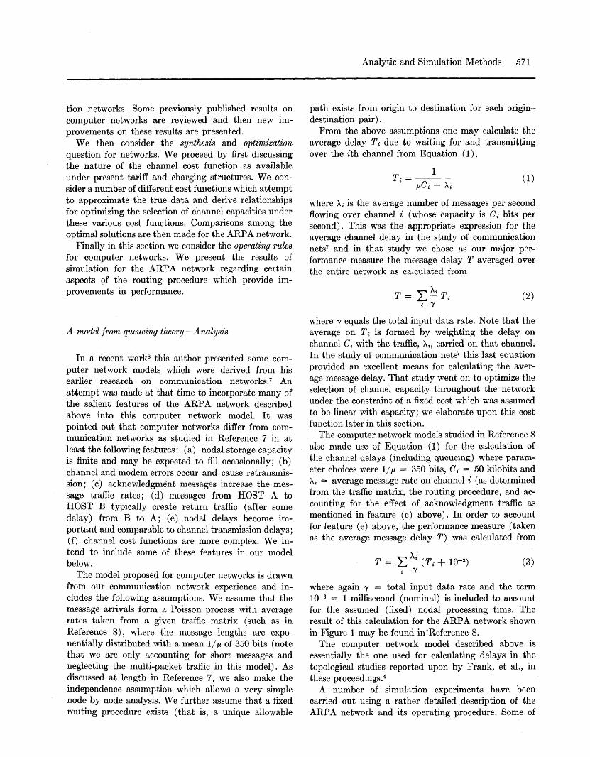
Figure 2—Comparison between theory and simulation for the ARPA network

these results were reported upon in Reference 8 and a comparison was made there between the theoretical results obtained from Equation (3) and the simulation results. This comparison is reproduced in Figure 2 where the lowest curve corresponds to the results of Equation (3). Clearly the comparison between simula­tion and theory is only mildly satisfactory. As pointed out in Reference 8, the discrepancy is due to the fact that the acknowledgment traffic has been improperly included in Equation (3). An attempt was made in Reference 8 to properly account for the acknowledg­ment traffic; however, this adjustment was unsatis­factory. The problem is that the average message length has been taken to be 350 bits and this length has averaged the traffic due to acknowledgment messages along with traffic due to real messages. These acknowl­edgments should not be included among those messages whose average system delay is being calculated and yet acknowledgment traffic must be included to properly account for the true loading effect in the network. In fact, the appropriate way to include this effect is to recognize that the time spent waiting for a channel is dependent upon the total traffic (including acknowledg­ments) whereas the time spent in transmission over a channel should be proportional to the message length of the real message traffic. Moreover, our theoretical

equations have accounted only for transmission delays which come about due to the finite rate at which bits may be fed into the channel (i.e., 50. kilobits per second); we are required however to include also the propagation time for a bit to travel down the length of the channel. Lastly, an additional one millisecond delay is included in the final destination node in order to deliver the message to the destination HOST. These additional effects give rise to the following expression for the average message delay T.

T= E + ^i/v-Ci

nCi — \i PLi + 10-3) + 10-

(4)

where 1/V = 560 bits (a real message's average length) and PLi is the propagation delay (dependent on the channel length, Li) for the *th channel. The first term in parentheses is the average transmission time and the second term is the average waiting time. The result of this calculation for the ARPA network gives us the curve in Figure 2 labeled "theory with correct acknowl­edge adjustment and propagation delays." The corre­spondence now between simulation and theory is un­believably good and we are encouraged that this ap­proach appears to be a suitable one for the prediction of computer network performance for the assumptions made here. In fact, one can go further and include the effect on message delay of the priority given to acknowl­edgment traffic in the ARPA network; if one includes this effect, one obtains another excellent fit to the simulation data labeled in Figure 2 as "theory cor­rected and with priorities."

As discussed in Reference 8 one may generalize the model considered herein to account for more general message length distributions by making use of the Pollaczek-Khinchin formula for the delay Ti of a

TABLE 1—Publicly Available Leased Transmission Line Costs from Reference 3

Speed

45 bps 56 bps 75 bps

2400 bps 41 KB 82 KB

230 KB 1 MB

12 MB

Cost/mile/month (normalized to

1000 mile distance)

$ .70 .70 .77

1.79 15.00 20.00 28.00 60.00

287.50

Analytic and Simulation Methods 573

channel with capacity d, where the message lengths have mean 1/p bits with variance <r2, where X* is the average message traffic rate and />* = \i/nCi which states

1 Ti = ——h

Pi(l + A 2 ) (5)

This expression would replace the first two terms in the parenthetical expression of Equation (4); of course by relaxing the assumption of an exponential distribu­tion we remove the simplicity provided by the Marko-vian property of the traffic flow. This approach, how­ever, should provide a better approximation to the true behavior when required.

Having briefly considered the problem of analyzing computer networks with regard to a single performance measure (average message delay), we now move on to the consideration of synthesis questions. This in­vestigation immediately leads into optimal synthesis procedures.

Optimization for various channel cost functions— Synthesis

We are concerned here with the optimization of the channel capacity assignment under various assump­tions regarding the cost of these channels. This opti­mization must be made under the constraint of fixed cost. Our problem statement then becomes:*

Select the {d} so as to minimize T

subject to a fixed cost constraint (6)

where, for simplicity, we use the expression in Equa­tion (2) to define T.

We are now faced with choosing an appropriate cost function for the system of channels. We assume that the total cost of the network is contained in these channel costs where we certainly permit fixed termina­tion charges, for example, to be included. In order to get a feeling for the correct form for the cost function let us examine some available data. From Reference 3 we have available the costing data which we present in Table 1. From a schedule of costs for leased com­munication lines available at Telpak rates we. have the data presented in Table 2.

We have plotted these functions in Figure 3. We

* The dual to this optimization problem may also be considered: "Select the {C,} so as to minimize cost, subject to a fixed message delay constraint." The solution to this dual problem gives the optimum C»- with the same functional dependence on X» as one obtains for the original optimization problem.

TABLE 2—Estimated Leased Transmission Line Costs Based on Telpak Rates.*

Cost Cost/mile/month (termination + mileage) (normalized to

Speed /month 1000 mile distance)

150 2400 7200

19.2 50

108 230.4 460.8

bps bps bps KB KB KB KB KB

1.344 MB

f 77.50 + $ .12/mile 232 810 850 850

2400 1300 1300 500

+ .35/mile + .35/mile + 2.10/mile + 4.20/mile + 4.20/mile + 21.00/mile + 60.00/mile + 75.00/mile

$ .20 .58

1.16 2.95 5.05 6.60

22.30 61.30 80.00

*These costs are, in some cases, first estimates and are not to be considered as quoted rates.

must now attempt to find an analytic function which fits cost functions of this sort. Clearly that analytic function will depend upon the rate schedule available to the computer network designer and user. Many analytic fits to this function have been proposed and in particular in Reference 3 a fit is proposed of the form:

Cost of line = 0.1C?-44 $/mile/month (7)

Based upon rates available for private line channels, Mastromonaco10 arrives at the following fit for line costs where he has normalized to a distance of 50 miles (rather than 1000 miles in Equation (7))

Cost of line = 1.08C?-316 $/mile/month (8)

Referring now to Figure 3 we see that the mileage

FROM TABLE I

ooro

I I I l l l l l l I I I Hl l l l » ' » ' " I I I I I I I I I I I 10* 10s

CAPACITY (bp»)

Figure 3—Scanty data on transmission line costs: $/mile/month normalized to 1000 mile distance

574 Spring Joint Computer Conference, 1970

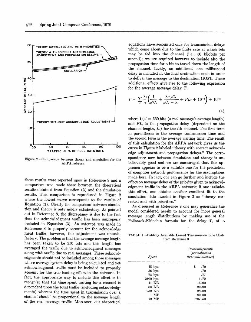
costs from Table 2 rise as a fractional exponent of capacity (in fact with an exponent of .815) suggesting the cost function shown in Equation (9) below

Cost of line = Ad°-m $/mile/month (9)

These last three equations give the dollar cost per mile per month where the capacity C» is given in bits per second. It is interesting to note that all three functions are of the form

Cost of line = ACf $/mile/month (10)

It is clear from these simple considerations that the cost function appropriate for a particular application depends upon that application and therefore it is difficult to establish a unique cost function for all situations. Consequently, we satisfy ourselves below by considering a number of possible cost functions and study optimization conditions and results which follow from those cost functions. The designer may then choose from among these to match his given tariff schedule. These cost functions will form the fixed cost constraint in Equation (6). Let us now consider the collection of cost functions, and the related optimiza­tion questions.

1. Linear cost function. We begin with this case since the analysis already exists in the author's Reference 7, where the assumed cost constraint took the form

D= J^diCi (11) i

where D = total number of dollars available to spend on channels, di = the dollar cost per unit of capacity on the ith channel, and d once again is the capacity of the ith. channel. Clearly Equation (11) is of the same form as Equation (10) with a = 1 where we now consider the cost of all channels in the system as having a linear form. This cost function assumes that cost is strictly linear with respect to capacity; of course this same cost function allows the assumption of a constant (for example, termination charges) plus a linear cost function of capacity. This constant (termination charge) for each channel may be subtracted out of total cost, D, to create an equivalent problem of the form given in Equation (11). The constant, di, allows one to account for the length of the channel since di may clearly be proportional to the length of the channel as well as anything else regarding the particular channel involved such as, for example, the terrain over which the channel must be placed. As was done in Reference 7, one may carry out the minimization given by Equa­tion (6) using, for example, the method of Lagrangian undetermined multipliers.5 This procedure yields the

following equation for the capacity

M \di / 2^ V%- dj j

where

D. = D-Z—>0 (13) i M

When we substitute this result back into Equation (2) we obtain that the performance measure for such a channel capacity assignment is

where

Ex/ * X

n — == - = average path length (15) 7 7

The resulting Equation (12) is referred to as the square root channel capacity assignment; this particular assignment first provides to each channel a capacity equal to Xi/n which is merely the average bit rate which must pass over that channel and which it must obviously be provided if the channel is to carry such traffic. In addition, surplus capacity (due to excess dollars, De) is assigned to this channel in proportion to the square root of the traffic carried, hence the name. In Reference 7 the author studied in great detail the particular case for which di = 1 (the case for which all channels cost the same regardless of length) and considerable information regarding topological design and routing procedures was thereby obtained. How­ever, in the case of the ARPA network a more reason­able choice for di is that it should be proportional to the length Lf of the ith channel as indicated in Equation (10) (for a = 1) which gives the per mileage cost; thus we may take di = A Li. This second case was con­sidered in Reference 8 and also in Reference 9. The interpretation for these two cases regarding the de­sirability of concentrating traffic into a few large and short channels as well as minimizing the average length of lines traversed by a message was well discussed and will not be repeated here.

We observe in the ARPA network example since the channel capacities are fixed at 50 kilobits that there is no freedom left to optimize the choice of channel capacities; however it was shown in Reference 8 that one could take advantage of the optimization procedure in the following way: The total cost of the network

Analytic and Simulation Methods 575

using 50 kilobit channels may be calculated. One may then optimize the network (in the sense of minimizing T) by allowing the channel capacities to vary while maintaining the cost fixed at this figure. The result of such optimization will provide a set of channel capac­ities which vary considerably from the fixed capacity network. It was shown in Reference 8 that one could improve the performance of the network in an efficient way by allowing that channel which required the largest capacity as a result of optimization to be increased from 50 kilobits in the fixed net to 250 kilobits. This of course increases the cost of the system. One may then provide a 250 kilobit channel for the second "most needy" channel from the optimization, increasing the cost further. One may then continue this procedure of increasing the needy channels to 250 kilobits while increasing the cost of the network and observe the way in which message delay decreases as system cost in­creases. I t was found that natural stopping points for this procedure existed at which the cost increased rapidly without a similar sharp decrease in message delay thereby providing some handle on the cost-performance trade-off.

Since we are more interested in the difference between results obtained when one varies the cost function in more significant ways, we now study additional cost functions.

2. Logarithmic cost functions. The next case of interest assumes a cost function of the form

D = J^dilogeOtCi (16) i

where D again is the total dollar cost provided for constructing the network, di is a coefficient of cost which may depend upon length of channel, a is an appropriate multiplier and C» is the capacity of the ith channel. We consider this cost function for two reasons: first-, because it has the property that the in­cremental cost per bit decreases as the channel size increases; and secondly, because it leads to simple theoretical results. We now solve the minimization problem expressed in Equation (6) where the fixed cost constraint is now given through Equation (16). We obtain the following equation for the capacity of the ith. channel

c'-;h^+(ii+(di)Y\ (17)

In this solution the Lagrangian multiplier /3 must be adjusted so that Equation (16) is satisfied when C» is substituted in from Equation (17). Note the unusual simplicity for the solution of C», namely that the channel capacity for the ith. channel is directly proportional to the traffic carried by that channel, X*//z- Contrast this

result with the result in Equation (12) where we had a square root channel capacity assignment. If we now take the simple result given in Equation (17) and use it in Equation (2) to find the performance measure T we obtain

r - ? U + l£ + faii)J) (18)

In this last result the performance measure depends upon the particular distribution of the internal traffic {Xt/ju} through the constant /3 which is adjusted as described above.

3. The power law cost function. As we saw in Equa­tions (7), (8), and (9) it appears that many of the existing tariffs may be approximated by a cost function of the form given in Equation (19) below.

D = Z did* (19) i

where a is some appropriate exponent of the capacity and di is an arbitrary multiplier which may of course depend upon the length of the channel and other perti­nent channel parameters. Applying the Lagrangian again with an undetermined multiplier /3 we obtain as our condition for an optimal channel capacity the following non-linear equation:

d--- Cp-o^gi = 0 (20) M

where

\M7i3o: dj

Once again, /J must be adjusted so as to satisfy the constraint Equation (19).

It can be shown that the left hand side of Equation (20) represents a convex function and that it has a unique solution for some positive value C;. We assume that a is in the range

0 < a < 1

as suggested from the data in Figure 3. We may also show that the location of the solution to Equation (20) is not especially sensitive to the parameter settings. Therefore, it is possible to use any efficient iterative technique for solving Equation (20) and we have found that such techniques converge quite rapidly to the optimal solution.

4. Comparison of solutions for various cost functions. In the last three subsections we have considered three different cost functions: the linear cost function; the logarithmic cost function; and the power law cost function. Of course we see immediately that the linear

576 Spring Joint Computer Conference, 1970

60 70 80 90 100 110 120 130 140 PERCENTAGE OF FULL DATA RATE

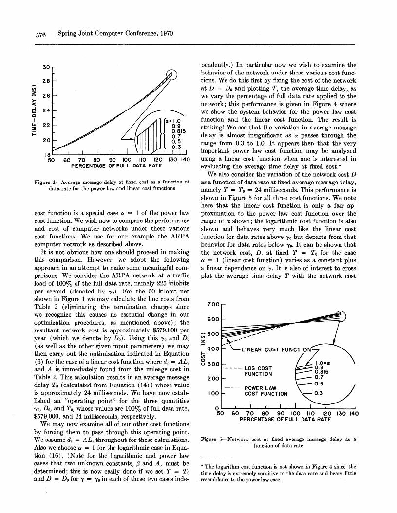
Figure 4—Average message delay at fixed cost as a function of data rate for the power law and linear cost functions

cost function is a special case a = 1 of the power law cost function. We wish now to compare the performance and cost of computer networks under these various cost functions. We use for our example the ARPA computer network as described above.

It is not obvious how one should proceed in making this comparison. However, we adopt the following approach in an attempt to make some meaningful com­parisons. We consider the ARPA network at a traffic load of 100% of the full data rate, namely 225 kilobits per second (denoted by 70). For the 50 kilobit net shown in Figure 1 we may calculate the line costs from Table 2 (eliminating the termination charges since we recognize this causes no essential change in our optimization procedures, as mentioned above); the resultant network cost is approximately $579,000 per year (which we denote by Do)- Using this 70 and D0

(as well as the other given input parameters) we may then carry out the optimization indicated in Equation (6) for the case of a linear cost function where di — ALi and A is immediately found from the mileage cost in Table 2. This calculation results in an average message delay T0 (calculated from Equation (14)) whose value is approximately 24 milliseconds. We have now estab­lished an "operating point" for the three quantities 70, Do, and T0, whose values are 100% of full data rate, $579,000, and 24 milliseconds, respectively.

We may now examine all of our other cost functions by forcing them to pass through this operating point. We assume di = ALi throughout for these calculations. Also we choose a = 1 for the logarithmic case in Equa­tion (16). (Note for the logarithmic and power law cases that two unknown constants, /3 and A, must be determined; this is now easily done if we set T = T0

and D = Do for 7 = 70 in each of these two cases inde­

pendently.) In particular now we wish to examine the behavior of the network under these various cost func­tions. We do this first by fixing the cost of the network at D = Do and plotting T, the average time delay, as we vary the percentage of full data rate applied to the network; this performance is given in Figure 4 where we show the system behavior for the power law cost function and the linear cost function. The result is striking! We see that the variation in average message delay is almost insignificant as a passes through the range from 0.3 to 1.0. I t appears then that the very important power law cost function may be analyzed using a linear cost function when one is interested in evaluating the average time delay at fixed cost.*

We also consider the variation of the network cost D as a function of data rate at fixed average message delay, namely T = T0 = 24 milliseconds. This performance is shown in Figure 5 for all three cost functions. We note here that the linear cost function is only a fair ap­proximation to the power law cost function over the range of a shown; the logarithmic cost function is also shown and behaves very much like the linear cost function for data rates above 70 but departs from that behavior for data rates below 70. It can be shown that the network cost, D, at fixed T = T0 for the case a = 1 (linear cost function) varies as a constant plus a linear dependence on 7. I t is also of interest to cross plot the average time delay T with the network cost

700 1-

50 60 70 80 90 100 110 120 130 140 PERCENTAGE OF FULL DATA RATE

Figure 5—Network cost at fixed average message delay as a function of data rate

* The logarithm cost function is not shown in Figure 4 since the time delay is extremely sensitive to the data rate and bears little resemblance to the power law case.

Analytic and Simulation Methods 577

D. This we do in Figure 6 for the class of power law cost functions. In Figures 6a and 6b we obtain points along the vertical and horizontal axes corresponding to fixed delay and fixed cost, respectively. These loci are obtained by varying y and we connect the points for equal y with straight lines as shown in the figure (how­ever, we in no way imply that the system passes along these straight lines as both T and D are allowed to vary simultaneously). We note the increased range of D as a varies from 0.3 to 1.0, but very little change in the range of T. In Figure 6c we collect together the behavior in this plane for many values of a where the lines labeled with a particular value of a correspond to the 50% data rate case in the lower left-hand portion of the figure and to the 130% data rate case in the upper right-hand portion of the figure. From Figure 6c we clearly observe that for fixed cost the time delay range varies insignificantly as a changes (as we emphasized in discussing Figure 4). Similarly, we observe the moderate variation at fixed time delay of network cost as a ranges through its values (this we saw clearly in Figure 5).

These studies of network optimization for various cost functions need further investigation. Our aim in this section has been to exhibit some of the performance characteristics under these cost functions and to com­pare them in some meaningful way.

Simulated routing in the ARPA network—Operating procedure

We have examined analysis and synthesis procedures for computer networks above. We now proceed to exhibit some properties of the network operating pro­cedure, in particular, the message routing procedure.

The ARPA network uses a routing procedure which is local in nature as opposed to global. Some details of this procedure are available in Reference 6 in these proceedings and we wish to comment on the method used for updating the routing tables. For purposes of routing, each node maintains a list which contains for each destination an estimate of the delay a message would encounter in attempting to reach that destina­tion node were it to be sent out over a particular channel emanating from that node; the list contains an entry for each destination and each line leaving the node in which this list is contained. Every half second (ap­proximately) each node sends to all of its immediate neighbors a list which contains its estimate of the shortest delay time to pass to each destination; this list therefore contains a number of entries which is one less than the number of nodes in the network. Upon receiving this information from one of its neighbors,

'18 20 22 24 26 28 18 20 22 24 26 28 30 TIME-DELAY (MS)

Figure 6—Locus of system performance for the power law cost function

the IMP adds to this list of estimated delays a measure of the current delays in passing from itself to the neigh­bor from whom it is receiving this list; this then pro­vides that IMP an estimate of the minimum delay required to reach all destinations if one traveled out over the line connected to that neighbor. The routing table for the IMP is then constructed by combining the lists of all of its neighbors into a set of columns and choosing as the output line for messages going to a particular destination that line for which the estimated delay over that line to that destination is minimum. What we have here described is essentially a periodic or synchronous updating method for the routing tables as currently used in the ARPA network. It has the clear advantages of providing reasonably accurate data regarding path delays as well as the important advantage of being a rather simple procedure both from an operational point of view and from an over­head point of view in terms of software costs inside the IMP program.

We suggest that a more efficient procedure in terms of routing delays is to allow asynchronous updating; by this we mean that routing information is passed from a node to its nearest neighbors only when signifi­cant enough changes occurr in its own routing table to warrant such an information exchange. The defini­tion of "significant enough" must be studied carefully

578 Spring Joint Computer Conference, 1970

200

1150

PlOO

50 -

LOOPS NOT SUPPRESSED -

LOOPS SUPPRESSED

FASTEST ZERO-LOAD PATH FIXED ROUTING - \

SYNCHRONOUS UPDATING

ASYNCHRONOUS UPDATING

1.0 2.0 3.0

AVERAGE PATH LENGTH

4.0 5.0

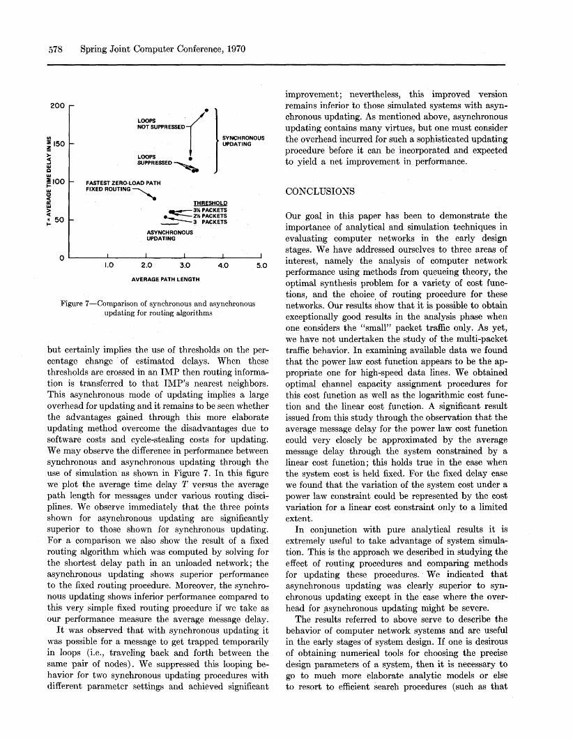
Figure 7—Comparison of synchronous and asynchronous updating for routing algorithms

but certainly implies the use of thresholds on the per­centage change of estimated delays. When these thresholds are crossed in an IMP then routing informa­tion is transferred to that IMP's nearest neighbors. This asynchronous mode of updating implies a large overhead for updating and it remains to be seen whether the advantages gained through this more elaborate updating method overcome the disadvantages due to software costs and cycle-stealing costs for updating. We may observe the difference in performance between synchronous and asynchronous updating through the use of simulation as shown in Figure 7. In this figure we plot the average time delay T versus the average path length for messages under various routing disci­plines. We observe immediately that the three points shown for asynchronous updating are significantly superior to those shown for synchronous updating. For a comparison we also show the result of a fixed routing algorithm which was computed by solving for the shortest delay path in an unloaded network; the asynchronous updating shows superior performance to the fixed routing procedure. Moreover, the synchro­nous updating shows inferior performance compared to this very simple fixed routing procedure if we take as our performance measure the average message delay.

I t was observed that with synchronous updating it was possible for a message to get trapped temporarily in loops (i.e., traveling back and forth between the same pair of nodes). We suppressed this looping be­havior for two synchronous updating procedures with different parameter settings and achieved significant

improvement; nevertheless, this improved version remains inferior to those simulated systems with asyn­chronous updating. As mentioned above, asynchronous updating contains many virtues, but one must consider the overhead incurred for such a sophisticated updating procedure before it can be incorporated and expected to yield a net improvement in performance.

CONCLUSIONS

Our goal in this paper has been to demonstrate the importance of analytical and simulation techniques in evaluating computer networks in the early design stages. We have addressed ourselves to three areas of interest, namely the analysis of computer network performance using methods from queueing theory, the optimal synthesis problem for a variety of cost func­tions, and the choice of routing procedure for these networks. Our results show that it is possible to obtain exceptionally good results in the analysis phase when one considers the "small" packet traffic only. As yet, we have not undertaken the study of the multi-packet traffic behavior. In examining available data we found that the power law cost function appears to be the ap­propriate one for high-speed data lines. We obtained optimal channel capacity assignment procedures for this cost function as well as the logarithmic cost func­tion and the linear cost function. A significant result issued from this study through the observation that the average message delay for the power law cost function could very closely be approximated by the average message delay through the system constrained by a linear cost function; this holds true in the case when the system cost is held fixed. For the fixed delay case we found that the variation of the system cost under a power law constraint could be represented by the cost variation for a linear cost constraint only to a limited extent.

In conjunction with pure analytical results it is extremely useful to take advantage of system simula­tion. This is the approach we described in studying the effect of routing procedures and comparing methods for updating these procedures. We indicated that asynchronous updating was clearly superior to syn­chronous updating except in the case where the over­head for asynchronous updating might be severe.

The results referred to above serve to describe the behavior of computer network systems and are useful in the early stages of system design. If one is desirous of obtaining numerical tools for choosing the precise design parameters of a system, then it is necessary to go to much more elaborate analytic models or else to resort to efficient search procedures (such as that

Analytic and Simulation Methods 579

described in Reference 4) in order to locate optimal designs.

ACKNOWLEDGMENTS

The author is pleased to acknowledge Gary L. Fultz for his assistance in simulation studies as well as his contributions to loop suppression in the routing pro­cedures; acknowledgment is also due to Ken Cher}, for his assistance in the numerical solution for the per­formance under different cost function constraints.

REFERENCES

1 S CARR S CROCKER V C E R F Host to host communication protocol in the ARPA network These proceedings

2 P A DICKSON ARPA network will represent integration on a large scale Electronics pp 131-134 September 30 1968

3 R G GOULD Comments on generalized cost expressions for private-line communications channels I E E E Transactions on Communication Technology V Com-13 No 3 pp 374-377 September 1965 also R P E C K H E R T P M KELLY A program for the development of a computer resource sharing network Internal Report for Kelly Scientific Corp Washington D C February 1969

4 H FRANK I T FRISCH W CHOU Topological considerations in the design of the ARPA computer network These proceedings

5 F B HILDEBRAND Methods of applied mathematics Prentice-Hall Inc Englewood Cliffs N J 1958

6 F E HEART R E KAHN S M ORNSTEIN W R CROWTHER D C WALDEN The interface message processor for the ARPA network These proceedings

7 L KLEINROCK Communication nets; stochastic message flow and delay McGraw-Hill New York 1964

8 L KLEINROCK Models for computer networks Proc of the International Communications Conference pp 21-9 to 21-16 University of Colorado Boulder June 1969

9 L KLEINROCK Comparison of solutions methods for computer network models Proc of the Computers and Communications Conference Rome New York September 30-October 2 1969

10 F R MASTRQMONACO Optimum speed of service in the design of customer data communications systems Proc of the ACM Symposium on the Optimization of Data Communications Systems pp 127-151 Pine Mountain Georgia October 13-16 1969

11 L G ROBERTS Multiple computer networks and intercomputer communications ACM Symposium on Operating Systems Principles Gatlinburg Tennessee October 1967

12 L G ROBERTS B D WESSLER Computer network developments to achieve resource sharing These proceedings