BIOMETRICS 57, 571-576 June 2001

Analyte Identification in Multivariate Calibration

Geoffrey Jones Institute of Information Sciences and Technology, Massey University,

Palmerston North, New Zealand

and

David M. Rocke Center for Image Processing and Integrated Computing, University of California, Davis, California 95616, U.S.A.

email: dmrocke@ucdavis.edu

SUMMARY. In calibration experiments, an estimated relationship between covariate information for a sam- ple and an observed response is used to infer the covariate information for unknown samples from their responses. In some situations, this covariate information comprises a nominal variable (e.g., identity of a chemical, sex of an animal) and a real-valued variable (e.g., concentration of the chemical, age of animal). If the calibrating relationship can be estimated separately for each candidate identity, the first step in analyzing unknown samples is to correctly determine their identity. A discrimination statistic is suggested for use in this situation and its asymptotic distribution is derived. The investigation is motivated by the possibility of using multiple immunoassays in environmental monitoring to identify and quantitate contaminated samples in situations where there are several candidate pollutants that cross-react significantly t o single assays. An example is given of the use of a four-antibody assay for the simultaneous monitoring of the levels in water samples of several of the commonly used triazine herbicides and their derivatives.

KEY WORDS: Cross-reactivity; Discrimination; Environmental monitoring; Four-parameter log-logistic model; Immunoassay; Multivariate calibration; Nonlinear regression.

1. Introduction Suppose we have a multivariate bioassay system in which the individual component assays are not specific for a particu- lar target analyte but respond with varying sensitivities to a number of different analytes. Such a situation can occur with immunoassays when antibodies developed for one target an- alyte cross-react significantly with other similar compounds. For example, in the environmental monitoring of the levels of s-triazine herbicides in water samples, it may be desirable to use an array of nonspecific immunoassays to detect, identify, and quantitate the members of this class of similar chemi- cals simultaneously. A simple example is illustrated in Figure 1, showing the bivariate response from a two-antibody sys- tem to varying concentrations of the herbicides atrazine and terbutryn together with the response from an unknown sam- ple. We wish to identify the chemical in the sample and esti- mate its concentration. Intuitively one might use the distance from the sample response to the response path specific to each chemical, but the metric for this distance must be chosen to incorporate what is known, or can be assumed, about the uncertainty in the responses. In reality, the class of possible analytes might be much larger. We have used the methods described here to investigate, in collaboration with chemists

and toxicologists, the use of an array of four antibodies for identifying eight s-triazines in water samples in concentra- tions of 0.5-100 ppb (parts per billion). Because our analysis extends to the possibility of simple mixtures of analytes, we denote the concentration by the r x 1 vector x so that, if we are looking for two-component mixtures, T = 2 and there are 28 possible identities.

We assume that the vector response of the assay system to concentration 2 of analyte j can be modeled as

Yj = f j ( O j , z ) + E , (1)

where yj is a q x 1 response vector, fj is a function assumed known to within a fixed p x 1 parameter vector O j , and E is a zero-mean error term. The dependence of fj on the analyte identity j may be only through the parameter vector O j , or it may be more general. We shall assume that E is normally distributed with positive-definite covariance matrix E.

Given training data {(yij, zij) : i = 1,. . . , nj} for each analyte identity j = 1,. . . , J , we can obtain consistent esti- mates dj of 0, and S of Z provided that certain smoothness and identifiability conditions are met. If we have an observed response from a sample of known identity but unknown con- centration, standard calibration theory may be used (Brown,

571

Biometrics. June 2001 572

0.8

0.7

0.6

0.5

0.4

0.3

0.2

0.1

0

0 Atrazine standards 8 Tnbutrynsta~~dards

Unknown sample

P d7

I d

B Y

0 0.1 0.2 0.3 0.4 0.5 0.6 0.7 0.8 *i 0.9

Figure 1. Response paths for atrazine and terbutryn as- sayed with two antibodies. Y1 and Y2 are the observed re- sponses (an optical density) from each of the two assays on two sets of standard concentrations and one unknown sample.

1993; Oman, 1999). Suppose, however, that we have an ob- served response yo from a sample for which the identity j and concentration z o are both unknown. We discuss in this article the problem of identifying the analyte by examining the compatibility of yo with estimated response curves Cj =

If we define the distance to the point on Cj at concentra- tion z as Rj(z) = [yo - f j (d j ,~ ) ]~S- ' [yo - fj(6j,z)], then the conditional least squares estimator of 20, assuming ana- lyte j , is the minimizer of this distance, hoj = argmin Rj(z). The use of this minimum value Rj ( P o j ) as a diagnostic statis- tic has been discussed in the literature for the case of linear calibration (Brown and Sundberg, 1989; Martens and Naes, 1989), but the distributional results used do not allow for un- certainty in the estimate 8. We discuss in Section 2 the nor- malization of this distance to allow for parameter uncertainty in the linear case. Extension to nonlinear calibration curves is considered in Section 3. In Section 4, we illustrate the use of the minimum normalized distance Rj* in the identification of s-triazine herbicides by multiple immunoarray.

The approach we take is to report all possible identities j for which R; is probabilistically small. If a point estimate of j were required, it would be natural to choose j so that Rj is minimized. The concentration ZO, conditional on the identity, could also be given as a point or interval estimate. These and other issues are discussed in Section 5 .

Details of proofs and simulations are omitted. The inter- ested reader is referred for these to Jones and Rocke (1997).

2. Linear Case Suppose we have a linear multivariate calibration experiment with training data (X,Y), where the responses Y form an n x q matrix, where each row is an independent observation of a q-variate response and the rows of the n x p design matrix X give the corresponding values of the p covariates. We assume the multivariate linear model Y = l n a T + XB + E, where aqXl is a vector of unknown constants, B p x q is the matrix of unknown slope parameters, and E n x q is an error matrix whose rows are independently distributed as N(Oq, X) , with

{fj(dj,Z) : z E B+T}, j = 1 , . . . , J .

X an unknown q x q positive definite covariance matrix. We assume further that the columns of X have been centered (i.e., that each covariate is measured from its mean) so that

We denote the usual estimates of the model parameters by 6, B, and S (cf., Anderson, 1984, pp. 287-291). Now suppose we have e replicates of an unknown with covariate values 20

and mean response yo. Brown (1982) showed that

XTln = 0,.

(yo - 6 - BTzo)TS-l(yo - h - BTz,) 5 1 + ; + z;(XTX)-Izo

q P N (n - p - 1) Fn -p- q . n - p - q

Williams (1959) suggested that, with the conditional least squares estimator 20 replacing 50, the above result holds with the numerator degrees of freedom in the F-distribution and scaling factor replaced by q - p. His suggestion seems to be based on the intuition that estimating the p parameters in z o will reduce the degrees of freedom by that amount. A more careful intuition notes the complementary effect on the denominator degrees of freedom, as in the derivation of the multivariate T 2 distribution (Anderson, 1984, pp. 161-162), and suggests the denominator degrees of freedom to be n - q. This is confirmed by the large-n a;symptotic expansions for R [yo - f (d , P)ITS-' [yo - f(0,2)] of Fujikoshi and Nishi (1984) and Davis and Hayakawa (1987). Their results, however, depend on 20, and they cannot justify replacing this by P o since the variance of PO does not decrease as n increases. We could circumvent this difficulty by insisting that f2 be large, but this severely limits the practical applicability of the result. Instead, we follow Brown and Sundberg (1987) in using small- sigma asymptotics so that our result applies for moderate amounts of training data and any number of replicates of unknowns, provided that the errors are reasonably small.

THEOREM 1 : Let X = m-'&, where XO is a fixed positive definite symmetric q x q matrix. Then, as m .+ 00, the statistic R* defined by

where PO = (BS-lBT)-lBS-lyo has

2, q - p P P FnZq R* - (n - p - 1)-

n - q (4)

and F:I;(.) denotes the F-distribution function with ( q - p) and (n - q) d.f.

The validity of this approximation depends on BE1/' be- ing large. This is similar to Brown's (1982) condition for in- evitability of a prediction region; intuitively, one requires the slope to be large relative to statistical uncertainty. Simula- tion suggests, however, that the approximation is remarkably good even for moderate-sized X. In practice, n will also be moderate sized so that the two asymptotic approaches work together.

If another estimator of X is available, such as is obtained by pooling S with the residuals from the unknowns, an analo- gous result is obtained by adjusting the denominator degrees of freedom in the F-distribution, provided that this estimator

Analyte Identification an Multivariate Calibration 573

is still independent of yo and B. If there are many additional degrees of freedom, then the distribution of R* can be re* sonably approximated by xi-,.

To investigate the practical applicability of our asymptotic result, simulation was used to generate empirical distribu- tions for R* and R, and these were compared with postu- lated distributions using the Kolmogorov-Smirnoff statistic max I&'(.) - F(.)l and the observed rates of exceedance of the nominal 95th and 99th percentiles for various values of n, q, p, and m. Williams's proposal for R* was compared with ours and a large-n simplification R* N x i F p ; we also investi- gated Brown and Sundberg's (1989) large-n asymptotic result

Full details of the simulation results are available in a tech- nical report (Jones and Rocke, 1997). To summarize, Wil- liams's proposal behaves poorly but expectedly less so as n gets larger. Our approximation, on the other hand, performs remarkably well even for small m (corresponding to large X): if all the slope parameters are O(l) , the approximation is good for m = 4. The large-n approximation to our result turns out to be inadequate until n approaches 50 and then only for small Q . Brown and Sundberg's (1989) asymptotic result us- ing R is not applicable when there is only a moderate amount of training data.

3. Nonlinear Extensions The general nonlinear multiresponse model (equation (1)) is very difficult to analyze since, unlike the linear case, estima- tion of cannot in general be separated from estimation of C and 6 and S are not independent. Analogous results to the linear case (equations (2) and (4)) appear to be intractable for the general nonlinear model. With appropriate regular- ity conditions (cf., Seber and Wild, 1989, pp. 581-585), the large-sample distribution of n1/2 (8 - 6 ) is asymptotically nor- mal with zero mean and a covariance matrix that can be esti- mated consistently from the data. However, using small-sigma asymptotics, with X = y-lZo, the asymptotic covariance matrix, VO say, of rn1/2(6 - 6 ) cannot be estimated consis- tently and neither can XO.

However, because of our assumption (equation (1)) that X does not depend on j , the calibration data for each analyte may be combined to give a pooled estimate of the variance. If there are many replicated unknowns, this further increases the degrees of freedom for S. Thus, the effective sample size for the estimation of X will often be much larger than that used in estimating 6. In such cases, we may treat Co as known, in which case VO is consistently estimated by mV, say, from the calibration data. The asymptotic distribution of m 1 / 2 [ f ( 6 , 50) - f (6, ZO)] is given via the delta method as N,(O, Go), where

R (1/l)Xgp.

is consistently estimated by replacing 8 by 8_and Vo by m V . Writing the estimator of the variance of f(6,zo) as G , it is easily seen that

which gives a nonlinear equivalent of equation (2). However,

the distributional result is now only approximate and depends on C being small.

Next we consider replacing zo by the conditional least squares estimator 20 to derive the distribution of a statis- tic for discriminating between candidate calibration models. In the simpler case where 8 is known, or estimated precisely, we have the following.

THEOREM 2: Let X = rn-lCo, where CO is a positive definite covariance matrix. Then, as m -+ oc), R = [yo -

V f (6 , *o)lTE-l [YO - f (0 , *0)1 - (lll)x&..

Finally, we consider how the above result is adapted to allow for uncertainty in the parameter estimate 8. Letting

where V is the estimated covariance of 6 , we have the follow- ing for the situation of Theorem 2.

THEOREM 3: R* = [yo - f(8,20)]T(!-1x + G)-'[y0 - f (8 , *o)l --$ v 2 xq - r .

The statistic R* again represents a normalized distance from the response of an unknown to an estimated calibra- tion model. It can be used as a diagnostic statistic to decide whether an unknown sample belongs to the same popula- tion as a set of calibration data, the population here being {f(z) E Wq : z E In the next section, we illustrate an application of the above results to the problem of determining the identity and concentration of contaminated environmental samples by multiple immunoassay.

4. Multiple Immunoassay 4.1 Single Unknown Analyte Immunoassay is a form of chemical analysis that uses antibodies to detect and quantitate a target compound or analyte. A common model (Rodbard, 1981) for the response Y at concentration x is

+ D ) + E , (6) A - D

log Y = log

where E N N(0, 02) , the log transform being applied to correct for heteroscedasticity and skewness.

It often happens that an antibody developed to bind specifically to a particular target molecule will also bind, perhaps less strongly, to similar molecules in the same class of compounds. The s-triazine herbicides, eg. , are a commonly used class of similar compounds, a number of which have been finding their way into ground water and may pose a human health hazard. Large-scale monitoring requires an assay methodology that, like immunoassay, is quick, precise, and cheap, but the development of completely specific antibodies for each member of the class is extremely costly and the subsequent monitoring of each by a different assay inefficient and slow.

One alternative is to use a panel of less specific antibodies to achieve simultaneous identification and quantitation. Our example uses four antibodies to discriminate between eight analytes. The format is such that standard concentrations of each candidate analyte are assayed together with unknown samples on a microtiter plate, as in Figure 2. One such

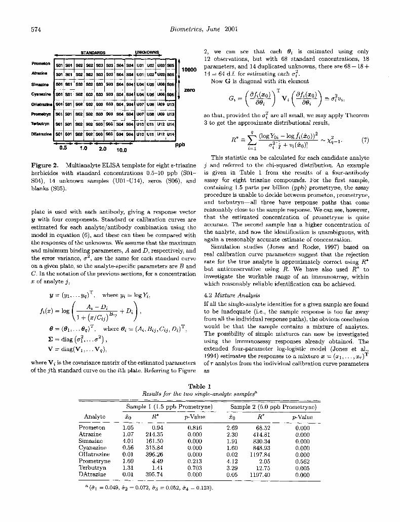
574 Biometrics, June 2001

UNKNOWNS c- STANDARDS

SO1 SO1 $02 SO2 SO3 503 SO4 SO4 U10 U11 U12 U14

SolISO1 I SOPI SO21 so31 so31 so4ls041 u10l U l l I u12lu14

10000 I f zero

Figure 2. Multianalyte ELISA template for eight s-triazine herbicides with standard concentrations 0.5-10 ppb (Sol- S04), 14 unknown samples (UOl-U14), zeros (S06), and blanks (S05).

plate is used with each antibody, giving a response vector y with four components. Standard or calibration curves are estimated for each analyte/antibody combination using the model in equation (6), and these can then be compared with the responses of the unknowns. We assume that the maximum and minimum binding parameters, A and D, respectively, and the error variance, u’, are the same for each standard curve on a given plate, so the analyte-specific parameters are B and C . In the notation of the previous sections, for a concentration x of analyte j,

T y = (y1, . . . yq ) , where yi = log y Z ,

8 = T , where& =(Ai,Bi j ,Ci j ,Di)T,

E = d i a g ( a l , 2 . . . u 2 ) ,

V = diag(V1 , . . . Vq),

where Vi is the covariance matrix of the estimated parameters of the j t h standard curve on the i th plate. Referring to Figure

2, we can see that each 8i is estimated using only 12 observations, but with 68 standard concentrations, 18 parameters, and 14 duplicated unknowns, there are 68 - 18 + 14 = 64 d.f. for estimating each uz.

Now G is diagonal with i th element

so that, provided the a? are all small, we may apply Theorem 3 to get the approximate distributional result,

This statistic can be calculated for each candidate analyte j and referred to the chi-squared distribution. An example is given in Table 1 from the results of a four-antibody assay for eight triazine compounds. For the first sample, containing 1.5 parts per billion (ppb) prometryne, the assay procedure is unable to decide between prometon, prometryne, and terbutryn-all three have response paths that come reasonably close to the sample response. We can see, however, that the estimated concentration of prometryne is quite accurate. The second sample has a higher concentration of the analyte, and now the identification is unambiguous, with again a reasonably accurate estimate of concentration.

Simulation studies (Jones and Rocke, 1997) based on real calibration curve parameters suggest that the rejection rate for the true analyte is approximately correct using R* but anticonservative using R. We have also used R* to investigate the workable range of an immunoarray, within which reasonably reliable identification can be achieved.

4.2 Mixture Analysis If all the single-analyte identities for a given sample are found to be inadequate (i.e., the sample response is too far away from all the individual response paths), the obvious conclusion would be that the sample contains a mixture of analytes. The possibility of simple mixtures can now be investigated using the immunoassay responses already obtained. The extended four-parameter log-logistic model (Jones et al.,

of r analytes from the individual calibration curve parameters as

1994) estimates the responses to a mixture s = (21,. . . , 2,) T

Table 1 Results f o r the two single-analyte samples”

Sample 1 (1.5 ppb Prometryne) Sample 2 (5.0 ppb Prometryne)

Analyte 20 R*

Prometon 1.05 0.94 Atrazine 1.07 214.35 Simazine 4.01 161.50 Cyanazine 0.56 315.84 OHatrazine 0.01 396.26 Prometryne 1.60 4.49 Terbutryn 1.31 1.41 DAtrazine 0.01 395.74

p-Value

0.816 0.000 0.000 0.000 0.000 0.213 0.703 0.000

R* pValue

2.69 2.30 1.91 1.60 0.02 4.12 3.29 0.05

68.52 414.81 830.34 848.93

1197.84 2.05

12.75 1197.40

0.000 0.000 0.000 0.000 0.000 0.562 0.005 0.000

~~

a (8, = 0.049, 82 = 0.072, 83 = 0.052, 84 = 0.123).

Analyte Identification in Multivariate Calibration 575

Table 2 Binary mixture analysis for 1

p p b atrazine + 1 ppb cyanazine

Analyte 1 Analyte 2 501 502 R* pValue

Atrazine Cyanazine 0.35 1.61 1.41 0.494 Simazine Cyanazine 0.38 1.84 1.28 0.527 Cyanazine DIatrazine 2.03 2.46 1.16 0.560

with

where Bf is the geometric mean of the slope parameters. If no single-analyte identity is found to be plausible for a

sample using the method of Section 4.1, we can next examine the possibility of two-component mixtures. We again search through the possible identities and test their plausibility using R* as defined in Theorem 3, now with r = 2.

This procedure has been investigated using binary mix- tures of 1 ppb of each of two analytes chosen from eight can- didate triazine compounds. Samples containing binary mix- tures of analytes are, as expected, more difficult to identify. Often there were a number of possible identities for the sam- ples, with the problem of confusion within subgroups being compounded. Thus, e.g., a mixture of atrazine and prometon might look like simazine and terbutryn or atrazine and prome- tryne. In most cases, mixtures were clearly identified as such, i.e., not as single analytes, although mixtures of prometon and terbutryn or prometryne and terbutryn were incorrectly classified as containing terbutryn only. Table 2 shows the ac- ceptable results for a mixture of 1 ppb atrazine with 1 ppb cynazine. There were 8 candidate analytes and thus 28 pos- sible binary mixtures. The computer searches through all 28, looking for acceptable solutions. There were three acceptable solutions found, one being the correct identity.

5. Discussion We have presented a statistic for discriminating between an- alytes in multivariate calibration and have derived an ap- proximating distribution using small-sigma asymptotics. This statistic incorporates uncertainty in the estimated model pa- rameters. In the nonlinear case, we have assumed a known co- variance matrix, which in some applications is not altogether unreasonable since it can be estimated much more precisely than can the individual model parameters. Extension to incor- porate the uncertainty in the covariance does not here seem to be as simple as merely substituting an F-distribution for a chi-squared, as is done in the linear case.

Our approach is based on the use of the classical or condi- tional least squares estimator for the unknown covariate 20. Brown and Sundberg (1987) showed that, in the linear case, the minimizer of equation (2) is actually the maximum like- lihood estimator, but simulations suggest that this is not a reliable way of getting the maximum likelihood estimation

(MLE) for nonlinear f ( . ) . Clarke (1992) uses a profile like- lihood method for the nonlinear case. A full maximum like- lihood analysis would be extremely complex with multiple unknowns, especially since the correct model for each is un- known. One could use the solution from our procedure as the starting point of a maximum likelihood analysis, perhaps proceeding sequentially by adding each unknown to the a p propriate calibration set to reestimate the parameters, then reapplying our procedure. Given, however, the discrete nature of the decisions being made (choice of analyte), it is easy to imagine such a system failing t o converge.

Our approach has been to report all possible identities com- patible with the data, i.e., for which Rj* is probabilistically small. Using this approach, we can find the range of concen- trations of each analyte for which reliable identification is pos- sible. For example, from the results of Table 1, we see that our immunoarray can distinguish prometryne at some concentra- tions but not others. In some applications, it may be necessary to make an unequivocal choice of identity, in which case one would choose the smallest R;, but the error rate will be high in cases where there is more than one plausible candidate. If prior information is available on the likelihood of the different analytes (e.g., application records in the herbicide example) this could easily be incorporated into the analysis. If inter- val estimates are required for the concentration in addition to the list of plausible analytes, R*(zo) of equation ( 5 ) could be used to determine a plausible range of concentrations for each analyte. Perhaps here a full Bayesian analysis would be preferable, with priors specified on the model parameters and on zcg as well as on the candidate analytes themselves. This is one direction of our future research in this area.

ACKNOWLEDGEMENTS This research was supported by the National Science Foun- dation (DMS 95-10511) and the National Institute for Envi- ronmental Health Science (P42 ES04699). We would like to thank Bruce Hammock and Monika Wortberg €or providing ELISA data. We are grateful to two referees and an associate editor for their careful reading of the original manuscript and for their helpful comments.

RESUMB Dans des experiences de calibration, une relation estimBe en- tre une information de type covariable pour un Cchantillon et une rBponse observee est utilisbe pour infBrer l’information covariable pour des Bchantillons pour lesquelles elle n’est pas connue 8. partir de leurs rkponses. Dans certaines situations, l’information covariable comprend une variable nominale (par exemple, identit6 d’un corps chimique, sexe d’un animal) et une variable 8. valeurs rBelles (par exemple, concentration du corps chimique, Bge de l’animal). Si la relation de calibration peut 6tre estimee sBparement pour chaque identit6 potentielle, la premikre &ape dans l’analyse d’Bchantillons inconnus est de determiner correctement leur identit6. Une statistique de dis- crimination est proposee pour traiter ce cas, et sa distribution asymptotique est calculbe. Le but de ce travail a BtB motive par la possibilitk, en suivi de l’environnement, d’utiliser des tests immunologiques multiples pour identifier et quantifier des Bchantillons contamin&, dans des situations ou il existe plusieurs polluants potentiels qui interagissent significative- ment dans des tests monofactoriels. Un exemple d’utilisation est donnk, avec un test utilisant quatre anticorps pour le suivi

576 Biometrics, June 2001

simultane du niveau de plusieurs triazines (herbicides) com- munement utilisees et de leurs derives dans des Bchantillons d'eau.

REFERENCES Anderson, T. W. (1984). An Introduction to Multivariate Sta-

tistical Analysis, 2nd edition. New York: Wiley. Brown, P. J. (1982). Multivariate calibration. Journal of the

Royal Statistical Society, Series B 44, 287-321. Brown, P. J. (1993). Measurement, Regression and Calibra-

tion. Oxford: Clarendon. Brown, P. J. and Sundberg, R. (1987). Confidence and conflict

in multivariate calibration. Journal of the Royal Statis- tical Society, Series B 49, 46-57.

Brown, P. J. and Sundberg, R. (1989). Prediction diagnostics and updating in multivariate Calibration. Biometrika 76,

Clarke, G. P. Y . (1992). Inverse estimates from a multire- sponse model. Biometrics 48, 1081-1094.

Davis, A. W. and Hayakawa, T. (1987). Some distribution theory relating to confidence regions in multivariate cal- ibration. Annals of the Institute of Statistical Mathemat-

349-361.

Jones, G. and Rocke, D. M. (1997). A discrimination statistic in multivariate calibration. Massey University Informa- tion and Mathematical Sciences Reports. Massey Uni- versity, New Zealand.

Jones, G., Wortberg, M., Kreissig, S. B., Gee, S. J., Ham- mock, B. D., and Rocke, D. M. (1994). Extension of the four-parameter logistic model for ELISA to multianalyte analysis. Journal of Immunological Methods 177, 1-7.

Martens, H. and Naes, T. (1989). Multivariate Calibration. New York: Wiley.

Oman, S. D. (1999). Multivariate calibration. In Multivariate Analysis, Design of Experiments, and Survey Sampling, S . Ghosh (ed). New York: Marcel Dekker.

Rodbard, D. (1981). Mathematics and statistics of ligand as- say: An illustrated guide. In Ligand Assay: Analysis of International Developments on Isotopic and Nonisotopic Immunoassay, J. Langan and J. J. Clapp (eds). New York: Masson.

Seber, G. A. F. and Wild, C. J. (1989). Nonlinear Regression. New York: Wiley.

Williams, E. J. (1959). Regression Analysis. New York: Wiley. Z C S 39, 141-152.

Fujikoshi, Y . and Nishi, R. (1984). On the distribution of a statistic in multivariate inverse regression analysis. Hi- roshima Mathematical Journal 14, 215-225.

Received October 1999. Revised August 2000. Accepted September 2000.