Analysisoftaskschedulingformulti-core embeddedsystems926952/FULLTEXT01.pdf ·...
118
Analysis of task scheduling for multi-core embedded systems Analys av schemaläggning för multikärniga inbyggda system JOSÉ LUIS GONZÁLEZ-CONDE PÉREZ, MASTER THESIS Examiner: Martin Törngren, KTH Supervisor: De-Jiu Chen, KTH Detlef Scholle, XDIN AB Barbro Claesson, XDIN AB MMK 2013:49 MDA 462
Transcript of Analysisoftaskschedulingformulti-core embeddedsystems926952/FULLTEXT01.pdf ·...
Analysis of task scheduling for multi-coreembedded systems
Analys av schemaläggning för multikärniga inbyggda system
JOSÉ LUIS GONZÁLEZ-CONDE PÉREZ, MASTER THESIS
Examiner:Martin Törngren, KTH
Supervisor:De-Jiu Chen, KTH
Detlef Scholle, XDIN ABBarbro Claesson, XDIN AB
MMK 2013:49 MDA 462


Acknowledgements
I would like to thank my supervisors Detlef Scholle and Barbro Claesson for givingme the opportunity of doing the Master thesis at XDIN. I appreciate the kindnessof Barbro chatting with me in Spanish and the support of Detlef no matter howmuch time it was required. I want to thank Sebastian, David and the other peopleat XDIN for the nice environment I lived in during these 20 weeks. I would like tothank the support and guidance of my supervisor at KTH DJ Chen and the helpof my examiner Martin Törngren in the last stage of the thesis.
I want to thank very much the other thesis colleagues at XDIN Joanna, Cheuk,Amir, Robin and Tobias. You have done this experience a lot more enriching. Iwould like to say merci! to my friends from Tyresö Benoit, Perrine, Simon, Audrey,Pierre, Marie-Line, Roberto, Alberto, Iván, Vincent, Olivier, Achour, Maxime, Si-mon, Emilie, Adelie, Siim and all the others. I have had great memories with youduring the first year at KTH. I thank Osman and Tarek for this year in Midsom-markransen.
I thank all the professors and staff from the Mechatronics department Mike,Bengt, Chen, Kalle, Jad and the others for making this programme possible, es-pecially Martin Edin Grimheden for his commitment with the students. I want tothank my friends from Mechatronics Eidur, René, Erik, Joanna, Marcus, Andreas,Mazda, Henrik, Oskar, Daniel and all the others. I would also like to thank otherfriends at KTH Lars, Hari, Maria, Sofia, Carl-Johan, Magnus, Ali and my tandemDaniel.
I want to thank my friends from Spain Héctor, Javi, Dani, Rubén, Raúl, Sil-via, Jesús, Emilio, Carolina, Marga, Belén, Juanjo, David, Luis and all the othersbecause you are a big part of my life.
Finally, I would like to thank the support of my parents Joselé and Maite andmy grandparents Domingo and Carmen because it makes me stronger in the difficulttimes. The love of my sisters Raquel and Cristina reminds me how lucky I am. Iwant to thank all my family because you have always given me the best.

AbstractThis thesis performs a research on scheduling algorithms for parallel appli-
cations. The main focus is their usage on multi-core embedded systems’ appli-cations. A parallel application can be described by a directed acyclic graph.A directed acyclic graph is a mathematical model that represents the parallelapplication as a set of nodes or tasks and a set of edges or communicationmessages between nodes.
In this thesis scheduling is limited to the management of multiple coreson a multi-core platform for the execution of application tasks. Tasks aremapped onto the cores and their start times are determined afterwards. Atoolchain is implemented to develop and schedule parallel applications on aEpiphany E16 developing board, which is a low-cost board with a 16 core chipcalled Epiphany. The toolchain is limited to the usage of offline schedulingalgorithms which compute a schedule before running the application.
The programmer has to draw a directed acyclic graph with the main at-tributes of the application. The toolchain then generates the code for the targetwhich automatically handles the inter-task communication. Some metrics areestablished to help evaluate the performance of applications on the target plat-form, such as the execution time and the energy consumption. Measurementson the Epiphany E16 developing board are performed to estimate the energyconsumption of the multi-core chip as a function of the number of idle cores.
A set of 12 directed acyclic graphs are used to verify that the toolchainworks correctly. They cover different aspects: join nodes, fork nodes, morethan one entry node, more than one exit node, different tasks weights anddifferent communication costs.
A use case is given, the development of a brake-by-wire demonstrationplatform. The platform aims to use the Epiphany board. Three experimentsare performed to analyze the performance of parallel computing for the usecase. Three brake-by-wire applications are implemented, one for a single coresystem and two for a multi-core system. The parallel application scheduledwith a list-based algorithm requires 266% more time and 1346% more energythan the serial application. The parallel application scheduled with a taskduplication algorithm requires 46% less time and 134% more energy than theserial application.
The toolchain system has proven to be a useful tool for developing paral-lel applications since it automatically handles the inter-task communication.However, future work can be done to automatize the decomposition of serialapplications from the source code. The conclusion is that this communicationsystem is suitable for coarse granularity, where the communication overheaddoes not affect so much. Task duplication is better to use for fine granularitysince inter-core communication is avoided by doing extra computations.

SammanfattningDetta examensarbete utför en studie av om schemaläggningsalgoritmer för
parallella applikationer. Huvudfokus är deras användning för flerkärniga in-byggda systemapplikationer. En parallell applikation kan beskrivas genom enriktad acyklisk graf. En riktad acyklisk graf är en matematisk modell somrepresenterar den parallella applikationen som en uppsättning av noder, elleruppgifter, och en uppsättning av pilar, eller meddelanden, mellan noder.
I denna uppsats är schemaläggning begränsad till hanteringen av flerakärnor på en multikärnig plattform för genomförandet av applikationens uppgif-ter. Uppgifter mappas på kärnorna och deras starttider bestäms efteråt. Enspeciell verktygskedja kallad ett ”toolchain system” har tagits fram för attutveckla och schemalägga parallella applikationer på ett Epiphany E16 kort,vilket är ett billigt kort med ett 16-kärnigt chip som kallas Epiphany. Toolchainsystemet är begränsat till användningen av offline schemaläggningsalgoritmersom beräknar ett schema innan du kör programmet.
Programmeraren måste rita en riktad acyklisk graf med de viktigaste at-tributen. Toolchain systemet genererar därefter kod som automatiskt hanterarkommunikationen mellan uppgifterna. Ett antal prestandamått defineras föratt kunna utvärdera applikationer på målplattformen, såsom genomförandetidoch energiförbrukning. Mätningar på Epiphany E16 kortet genomförs för attuppskatta energiförbrukningen som en funktion av antalet lediga kärnor.
En uppsättning av 12 riktade acykliska grafer används för att kontrolleraatt toolchain systemet fungerar korrekt. De täcker olika aspekter: noder somgår ihop, noder som går isär, fler än en ingångsnod, fler än en utgångsnod,olika vikter på uppgifterna och olika kommunikationskostnader.
Ett användningsfall ges, utveckling av en brake-by-wire demonstrationsplattform. Plattformen syftar till att använda Epiphany kortet. Tre experi-ment utförs för att analysera resultatet av parallella beräkningar för använd-ningsfallet. Tre brake-by-wire applikationer genomförs, en för ett enda kärn-system och två för ett multikärnigt system. Den parallella applikationen somvar schemalagd med en algoritm baserad på listor kräver 266% mer tid och1346% mer energi än den seriella applikationen. Den parallella applikationensom var schemalagd med en uppgiftsduplicerings-algoritm kräver 46% mindretid och 134% mer energi än den seriella applikationen.
Toolchain systemet har visat sig att vara ett användbart verktyg för attutveckla parallella applikationer eftersom det automatiskt hanterar kommu-nikation mellan uppgifter. Däremot kan framtida arbete göras för att automa-tisera nedbrytningen av seriella program från källkod. Slutsatsen är att dettakommunikationssystem är lämpligt för grovkorning parallellism, där kommu-nikationskostnaden inte påverkar lika mycket. Uppgiftsdupliceringen är bättreatt använda för finkorning parallellism eftersom kommunikation mellan kärnorundviks genom att göra extra beräkningar.

Contents
Contents
List of Figures
List of Tables
List of Abbreviations
I Analytical phase 1
1 Introduction 31.1 Background . . . . . . . . . . . . . . . . . . . . . . . . . . . . . . . . 31.2 Problem statement . . . . . . . . . . . . . . . . . . . . . . . . . . . . 41.3 System requirements . . . . . . . . . . . . . . . . . . . . . . . . . . . 51.4 Team goal . . . . . . . . . . . . . . . . . . . . . . . . . . . . . . . . . 51.5 Method . . . . . . . . . . . . . . . . . . . . . . . . . . . . . . . . . . 6
1.5.1 Analytical phase . . . . . . . . . . . . . . . . . . . . . . . . . 61.5.2 Practical phase . . . . . . . . . . . . . . . . . . . . . . . . . . 6
1.6 Delimitation . . . . . . . . . . . . . . . . . . . . . . . . . . . . . . . . 6
2 Use case description and requirements 92.1 Introduction to brake-by-wire . . . . . . . . . . . . . . . . . . . . . . 102.2 Use case description . . . . . . . . . . . . . . . . . . . . . . . . . . . 11
2.2.1 Control view . . . . . . . . . . . . . . . . . . . . . . . . . . . 112.2.2 Physical view . . . . . . . . . . . . . . . . . . . . . . . . . . . 12
2.3 Use case requirements . . . . . . . . . . . . . . . . . . . . . . . . . . 122.3.1 Real-time guarantees . . . . . . . . . . . . . . . . . . . . . . . 122.3.2 Fault-tolerance . . . . . . . . . . . . . . . . . . . . . . . . . . 122.3.3 Energy efficiency . . . . . . . . . . . . . . . . . . . . . . . . . 13
2.4 Summary . . . . . . . . . . . . . . . . . . . . . . . . . . . . . . . . . 13
3 Parallel computing 153.1 Introduction to parallel computing . . . . . . . . . . . . . . . . . . . 15
CONTENTS
3.1.1 Parallel system . . . . . . . . . . . . . . . . . . . . . . . . . . 153.2 Task models . . . . . . . . . . . . . . . . . . . . . . . . . . . . . . . . 16
3.2.1 Task model for independent tasks . . . . . . . . . . . . . . . . 163.2.2 Task model for interdependent tasks with communication costs 17
3.3 Examples of parallel applications . . . . . . . . . . . . . . . . . . . . 193.3.1 LU decomposition graph . . . . . . . . . . . . . . . . . . . . . 193.3.2 Laplace algorithm graph . . . . . . . . . . . . . . . . . . . . . 203.3.3 FFT algorithm graph . . . . . . . . . . . . . . . . . . . . . . 203.3.4 Stencil algorithm graph . . . . . . . . . . . . . . . . . . . . . 21
3.4 Application decomposition and dependency analysis . . . . . . . . . 213.5 Task scheduling . . . . . . . . . . . . . . . . . . . . . . . . . . . . . . 22
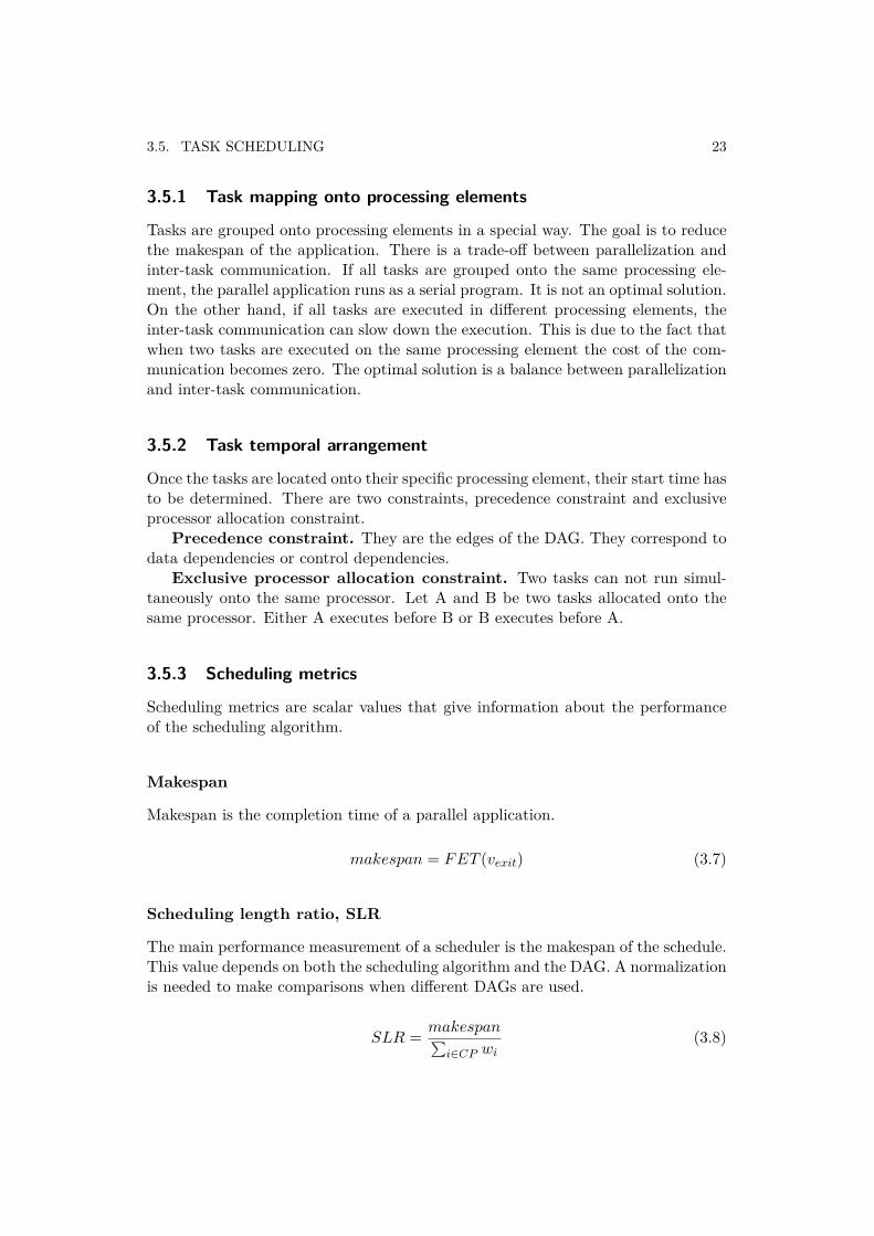
3.5.1 Task mapping onto processing elements . . . . . . . . . . . . 233.5.2 Task temporal arrangement . . . . . . . . . . . . . . . . . . . 233.5.3 Scheduling metrics . . . . . . . . . . . . . . . . . . . . . . . . 233.5.4 Optimality, feasibility and schedulability . . . . . . . . . . . . 24
3.6 Related technology . . . . . . . . . . . . . . . . . . . . . . . . . . . . 243.6.1 OpenMP . . . . . . . . . . . . . . . . . . . . . . . . . . . . . 243.6.2 MPI . . . . . . . . . . . . . . . . . . . . . . . . . . . . . . . . 253.6.3 OpenHMPP . . . . . . . . . . . . . . . . . . . . . . . . . . . . 253.6.4 OpenACC . . . . . . . . . . . . . . . . . . . . . . . . . . . . . 263.6.5 CAPS compilers and CodeletFinder . . . . . . . . . . . . . . 26
3.7 Summary . . . . . . . . . . . . . . . . . . . . . . . . . . . . . . . . . 27
4 Scheduling for interdependent tasks with communication costs 294.1 List-based algorithms . . . . . . . . . . . . . . . . . . . . . . . . . . 30
4.1.1 Highest level first with estimated times, HLFET . . . . . . . 304.1.2 Modified Critical Path, MCP . . . . . . . . . . . . . . . . . . 304.1.3 Earliest time first, ETF . . . . . . . . . . . . . . . . . . . . . 314.1.4 Dynamic Level Scheduling, DLS . . . . . . . . . . . . . . . . 314.1.5 Cluster ready Children First, CCF . . . . . . . . . . . . . . . 314.1.6 Hybrid Re-mapper minimum partial completion time Static
Priority, Hybrid Re-mapper PS . . . . . . . . . . . . . . . . . 314.2 Clustering algorithms . . . . . . . . . . . . . . . . . . . . . . . . . . 31
4.2.1 Edge-Zeroing or Single Edge, EZ or SE . . . . . . . . . . . . 334.2.2 Linear Clustering, LC . . . . . . . . . . . . . . . . . . . . . . 344.2.3 Dominant Sequence Clustering, DSC . . . . . . . . . . . . . . 354.2.4 Mobility Directed, MD . . . . . . . . . . . . . . . . . . . . . . 374.2.5 Dynamic Critical Path, DCP . . . . . . . . . . . . . . . . . . 37
4.3 Arbitrary processor network algorithms, APN . . . . . . . . . . . . . 384.3.1 Mapping Heuristic, MH . . . . . . . . . . . . . . . . . . . . . 394.3.2 Bottom-Up, BU . . . . . . . . . . . . . . . . . . . . . . . . . 40
4.4 Duplication algorithms . . . . . . . . . . . . . . . . . . . . . . . . . . 404.4.1 Contention-aware scheduling algorithm with task duplication 41
4.5 Summary . . . . . . . . . . . . . . . . . . . . . . . . . . . . . . . . . 42

CONTENTS
5 Discussion and conclusions for scheduling 435.1 Requirements analysis . . . . . . . . . . . . . . . . . . . . . . . . . . 435.2 Performance comparison . . . . . . . . . . . . . . . . . . . . . . . . . 455.3 Design decisions . . . . . . . . . . . . . . . . . . . . . . . . . . . . . 47
II Practical phase 49
6 System design and architecture: Toolchain 516.1 Graph editor . . . . . . . . . . . . . . . . . . . . . . . . . . . . . . . 516.2 Xgml parser module . . . . . . . . . . . . . . . . . . . . . . . . . . . 526.3 Clustering algorithm module . . . . . . . . . . . . . . . . . . . . . . 536.4 Code generator module . . . . . . . . . . . . . . . . . . . . . . . . . 546.5 Application development . . . . . . . . . . . . . . . . . . . . . . . . . 55
7 System design and architecture: Epiphany application 577.1 Epiphany module . . . . . . . . . . . . . . . . . . . . . . . . . . . . . 577.2 Interrupts module . . . . . . . . . . . . . . . . . . . . . . . . . . . . 587.3 File system module . . . . . . . . . . . . . . . . . . . . . . . . . . . . 607.4 Mailbox module . . . . . . . . . . . . . . . . . . . . . . . . . . . . . . 617.5 Host communication module . . . . . . . . . . . . . . . . . . . . . . 627.6 Profiler module . . . . . . . . . . . . . . . . . . . . . . . . . . . . . . 63
8 Implementation 658.1 Power management . . . . . . . . . . . . . . . . . . . . . . . . . . . . 658.2 Inter-core communication . . . . . . . . . . . . . . . . . . . . . . . . 66
9 Results 699.1 Toolchain testing . . . . . . . . . . . . . . . . . . . . . . . . . . . . . 699.2 Brake by wire application . . . . . . . . . . . . . . . . . . . . . . . . 719.3 Collected data . . . . . . . . . . . . . . . . . . . . . . . . . . . . . . 74
9.3.1 Power consumption’s data . . . . . . . . . . . . . . . . . . . . 749.3.2 Timers’ data . . . . . . . . . . . . . . . . . . . . . . . . . . . 749.3.3 Single core application’s data . . . . . . . . . . . . . . . . . . 759.3.4 Parallel application’s data . . . . . . . . . . . . . . . . . . . . 779.3.5 Parallel application with task duplication’s data . . . . . . . 79
9.4 Data analysis . . . . . . . . . . . . . . . . . . . . . . . . . . . . . . . 819.4.1 Timers analysis . . . . . . . . . . . . . . . . . . . . . . . . . . 819.4.2 Single core application analysis . . . . . . . . . . . . . . . . . 819.4.3 Parallel application analysis . . . . . . . . . . . . . . . . . . . 819.4.4 Parallel application with task duplication analysis . . . . . . 82
9.5 Requirements evaluation . . . . . . . . . . . . . . . . . . . . . . . . . 829.6 Summary . . . . . . . . . . . . . . . . . . . . . . . . . . . . . . . . . 83
10 Conclusions and future work 85

CONTENTS
10.1 Conclusions . . . . . . . . . . . . . . . . . . . . . . . . . . . . . . . . 8510.2 Limitations . . . . . . . . . . . . . . . . . . . . . . . . . . . . . . . . 8510.3 Future work . . . . . . . . . . . . . . . . . . . . . . . . . . . . . . . . 85
A Epiphany power consumption test application
B Brake-by-wire application: single core
C Brake-by-wire application: tasks
D Brake-by-wire application with task duplication: tasks
Bibliography

List of Figures
2.1 Design of automotive control applications . . . . . . . . . . . . . . . . . 92.2 Brake system technologies . . . . . . . . . . . . . . . . . . . . . . . . . . 102.3 Brake-by-wire control structure . . . . . . . . . . . . . . . . . . . . . . . 11
3.1 A sample Directed Acyclic Graph (DAG) . . . . . . . . . . . . . . . . . 183.2 Parallel algorithms . . . . . . . . . . . . . . . . . . . . . . . . . . . . . . 203.3 OpenMP parallelization . . . . . . . . . . . . . . . . . . . . . . . . . . . 253.4 OpenHMPP model . . . . . . . . . . . . . . . . . . . . . . . . . . . . . . 263.5 CodeletFinder . . . . . . . . . . . . . . . . . . . . . . . . . . . . . . . . . 273.6 CAPS compiler . . . . . . . . . . . . . . . . . . . . . . . . . . . . . . . . 27
4.1 List-based scheduling algorithms’ comparison, taken from [1]. B-rowsstand for better performance than the compared algorithm. E-rowsstand for equal performance as the compared algorithm. W-rows standfor worse performance than the compared algorithm. . . . . . . . . . . . 32
4.2 Edge-Zeroing . . . . . . . . . . . . . . . . . . . . . . . . . . . . . . . . . 344.3 Linear Clustering . . . . . . . . . . . . . . . . . . . . . . . . . . . . . . . 354.4 MD, MCP, DSC, DLS and DCP comparison . . . . . . . . . . . . . . . . 374.5 Arbitrary processor network algorithm . . . . . . . . . . . . . . . . . . . 384.6 Task duplication . . . . . . . . . . . . . . . . . . . . . . . . . . . . . . . 404.7 Origin duplication . . . . . . . . . . . . . . . . . . . . . . . . . . . . . . 414.8 Destination duplication . . . . . . . . . . . . . . . . . . . . . . . . . . . 41
6.1 Toolchain . . . . . . . . . . . . . . . . . . . . . . . . . . . . . . . . . . . 516.2 yEd graph . . . . . . . . . . . . . . . . . . . . . . . . . . . . . . . . . . . 526.3 Node and edge structures . . . . . . . . . . . . . . . . . . . . . . . . . . 526.4 Generated code . . . . . . . . . . . . . . . . . . . . . . . . . . . . . . . . 54
7.1 Software modules stack . . . . . . . . . . . . . . . . . . . . . . . . . . . 577.2 Board memory . . . . . . . . . . . . . . . . . . . . . . . . . . . . . . . . 587.3 Interrupt Service Routine (ISR) operation . . . . . . . . . . . . . . . . . 607.4 Fat_table and the Root_directory . . . . . . . . . . . . . . . . . . . . . 617.5 Send_message function . . . . . . . . . . . . . . . . . . . . . . . . . . . 627.6 Retrieve_message function . . . . . . . . . . . . . . . . . . . . . . . . . 62

7.7 Profiler functions . . . . . . . . . . . . . . . . . . . . . . . . . . . . . . . 63
8.1 Epiphany schematic . . . . . . . . . . . . . . . . . . . . . . . . . . . . . 66
9.1 Toolchain testing set . . . . . . . . . . . . . . . . . . . . . . . . . . . . . 699.2 Alternative DAG with shorter makespan . . . . . . . . . . . . . . . . . . 709.3 Brake-by-wire physical view . . . . . . . . . . . . . . . . . . . . . . . . . 719.4 Brake-by-wire epiphany application . . . . . . . . . . . . . . . . . . . . . 729.5 Brake-by-wire host application . . . . . . . . . . . . . . . . . . . . . . . 739.6 Epiphany power consumption . . . . . . . . . . . . . . . . . . . . . . . . 749.7 Brake-by-wire application (single core) . . . . . . . . . . . . . . . . . . . 769.8 Brake-by-wire application timing . . . . . . . . . . . . . . . . . . . . . . 789.9 Brake-by-wire application with task duplication . . . . . . . . . . . . . . 80
List of Tables
4.1 HLFET, MCP, ETF and DLS performance evaluation . . . . . . . . . . 314.2 MCP, ETF, MD and DSC comparison . . . . . . . . . . . . . . . . . . . 364.3 ETF, EZ and DSC performance evaluation . . . . . . . . . . . . . . . . 36
5.1 List-based algorithms and clustering algorithms: Performance comparison 465.2 Arbitrary processor network: Performance comparison . . . . . . . . . . 465.3 First prototype specification . . . . . . . . . . . . . . . . . . . . . . . . . 475.4 Ideal system specification . . . . . . . . . . . . . . . . . . . . . . . . . . 48
7.1 Me structure’s fields . . . . . . . . . . . . . . . . . . . . . . . . . . . . . 59
9.1 Summary of the evaluated aspects with each example DAG . . . . . . . 719.2 Single core application’s task and core profiler . . . . . . . . . . . . . . . 769.3 Single core application’s timing . . . . . . . . . . . . . . . . . . . . . . . 769.4 Parallel application’s core profiler . . . . . . . . . . . . . . . . . . . . . . 779.5 Number of idle cycles . . . . . . . . . . . . . . . . . . . . . . . . . . . . 779.6 Parallel application’s task profiler . . . . . . . . . . . . . . . . . . . . . . 799.7 Parallel application with task duplication’s core profiler . . . . . . . . . 809.8 Parallel application with task duplication’s task profiler . . . . . . . . . 809.9 Performance comparison between brake-by-wire applications . . . . . . . 84


List of Abbreviations
ABS Anti-lock Braking System
AEST Absolute Earliest Start Time
ALAP As Late As Possible
ALST Absolute Latest Start Time
AMP Asymmetric MultiProcessing
API Application Programming Interface
ARTEMIS Advanced Research & Technology for EMbedded Intelligence and Sys-tems
ASAP As Soon As Possible
CCR Communication to Computation Ration
CP Critical Path
CPU Central Processing Unit
DAG Directed Acyclic Graph
DL Dynamic Level
DMA Direct Memory Access
DS Dominant Sequence
ECU Electronic Control Unit
EEST Earliest Execution Start Time
ESP Electronic Stability Program
EST Earliest Start Time

LIST OF ABBREVIATIONS
FET Finishing Execution Time
FPU Floating-Point Unit
GPU Graphics Processing Unit
GUI Graphical User Interface
HWA HardWare Accelerator
ISR Interrupt Service Routine
ITEA2 Information Technology for European Advancement
IVT Interrupt Vector Table
LST Latest Start Time
MANY MANY-core programming and resource management for high-performanceembedded systems
MBAT combined Model-Based Analysis and Testing of embedded systems
MIMD Multiple Instruction, Multiple Data streams
MISD Multiple Instruction, Single Data stream
OS Operating System
PaPP Portable and Predictable Performance on heterogeneous embedded many-cores
RPC Remote Procedure Call
RTOS Real-Time Operating System
SIMD Single Instruction, Multiple Data streams
SISD Single Instruction, Single Data stream
SLR Scheduling Length Ratio
SMP Symmetric MultiProcessing
TCS Traction Control System
TG Topology Graph
Part I
Analytical phase
1


Chapter 1
Introduction
1.1 Background
The thesis work has been conducted at XDIN AB, an engineering and IT consultingfirm. The main customers belong to the energy, telecommunication, manufacturingand automotive industries. The thesis is part of the MANY-core programming andresource management for high-performance embedded systems (MANY), combinedModel-Based Analysis and Testing of embedded systems (MBAT) and Portable andPredictable Performance on heterogeneous embedded manycores (PaPP) projects.MANY is hosted by Information Technology for European Advancement (ITEA2).MBAT and PaPP are hosted by Advanced Research & Technology for EMbeddedIntelligence and Systems (ARTEMIS) (industry association and joint undertakingin the field of embedded systems).
Traditionally computing architectures have been made up of one processingunit. This paradigm was good enough to cope with the software requirements.Factors such as the growing software complexity and size or the amount of data tobe processed demanded processors with higher frequency. Hardware manufactureswere able to launch to the market faster processors until a limit was reached.
The dynamic power that a chip consumes is given by the equation P = ACV 2F .Where A is the activity factor, C is the switched capacitance, V is the supply voltageand F is the clock frequency. This means that the power consumed by the chipis proportional to the clock frequency. Therefore higher frequency processors aremore power greedy.
This is reflected by the fact that Intel canceled Tejas and Jayhawk processorsin May 2004 [2]. The power consumption of the chip became prohibitive. Anotherside effect was the increase of heat. The required architectures to dissipate the heatbecame too complex and expensive. Frequency scaling was not viable any more.
Chip makers such as Intel and AMD started to develop multi-core architec-tures. Multi-core architectures are composed of more than one processing unit.The speed up of the application is achieved by parallel computing, a new paradigmin programming. Applications are able to run faster in more energy efficient ar-
3

4 CHAPTER 1. INTRODUCTION
chitectures. However, effective parallel computing has a cost. It requires eithermore programming expertise or to develop automatic code generation tools [3]. Inthe first approach the programmer has to specify in the code which parts can beparallelized and on which processing elements they will run. The second approachis to come up with new tools that abstract the programmers from parallelizing theapplication and from scheduling it onto the platform. The goal is to go for thesecond approach but more work has to be done by the academy and the industryin order to cope with problems such as hardware heterogeneity.
Embedded systems are often required to be real-time and energy efficient. Theyare broadly used in space and military applications for executing specific tasks thatare time constrained. A wide range of control and signal processing applications inthe industry are run on them. They are also found in everyday life such as consumerelectronics.
Embedded systems with multi-core processors are growing due to the diversityof applications they can run. Industrial applications with high potential are ma-chine vision, CAD systems, CNC machines, automated test systems and motioncontrol [4]. Some of them do a lot of math computations over a given dataset andcan be decomposed into smaller tasks by applying data partitioning. Multi-coreplatforms are specially appropriate for battery-powered embedded systems. Multi-ple energy-efficient cores can give the same performance as a powerful core with asmaller budget of energy [5] and [6]. They also offer other benefits such as boundeddeterminism, dedicated CPU cores, decreased clock jitter, expanded resources forscaling and optimal contention for resources [7].
Parallel computing is a concept to be explored in the embedded systems’ world.A variety of new programming languages, compilers and scheduling strategies arearising for parallel computing ([8] and [9]). It is especially interesting the area ofscheduling. Scheduling has become a complex issue since there is now more than oneprocessing element. It handles the mapping of application tasks onto the processorsand the determination of their start times.
1.2 Problem statement
The first goal of the thesis is to make an in-depth study of the state of the artscheduling algorithms for parallel computing in embedded systems. The secondgoal is to design and implement a scheduling algorithm based on the previous studyto deploy tasks on the target platform for a brake-by-wire application.
The scheduler will be implemented in a Epiphany E16 developing board. Thefinal target is a low cost parallel platform called Parallella from Adapteva. The maincomponents of the architecture are a Xilinx Zynq7000 FPGA and the Epiphany chip.The Xilinx Zynq7000 has a Dual-Core ARM-A9 programmed inside and a bus tocommunicate to the Epiphany chip. The Epiphany chip is a 16-core co-processor.It contains an e-Mesh Network-on-Chip which connects a 2D array of e-Nodes.
The demonstration platform is made up of one Epiphany E16 developing board

1.3. SYSTEM REQUIREMENTS 5
among other things. Communication between tasks will be based on message pass-ing. The following questions are of special interest:
• Which scheduling algorithm is going to be used? Why?
• Which metrics are going to be used to measure the performance of the sched-uler?
1.3 System requirementsThis section states the requirements that the ideal scheduler should fulfill. Theserequirements were set up during the whole analytical phase. To set up the require-ments it was necessary to have a good understanding of scheduling and parallelcomputing. Chapter 5 will elaborate and clarify the requirements. The aim ofthe thesis is to design and implement a system that complies with the followingrequirements:
REQ_1 The scheduler shall cope with both serial and parallel applications.
REQ_2 The scheduler shall do automatic parallelization of the application. Par-allelization shall be transparent to the programmer.
REQ_3 The scheduler shall parallelize tasks as much as possible.
REQ_4 The scheduler shall avoid communication as much as possible.
REQ_5 The scheduler shall provide to an application an end-to-end guarantee.An end-to-end guarantee is a kind of timing requirement that might be givenby a control requirement of the application, such as stability or settling time.
REQ_6 The scheduler shall generate a schedule with the minimum execution time.
REQ_7 The scheduler shall be energy efficient.
REQ_8 The scheduler shall be target independent. The algorithm shall be easilyportable to other platforms.
Some of the requirements, such as REQ_3 and REQ_4, may actually be inconflict. Section 5.1 will present how this requirements can be fulfilled and to whichdegree.
1.4 Team goalThere are four master thesis workers at XDIN in the spring of 2013, all workingseparately but within the same topic. The goal for the team is to in the end com-bine their knowledge and implement their respective work on the same distributedembedded system. The aim is to implement a brake-by-wire system based on a newmiddle-ware layer.

6 CHAPTER 1. INTRODUCTION
1.5 Method
The thesis is split into two main phases: the analytical part and the practical part.
1.5.1 Analytical phase
A study about task scheduling on a multi-core embedded system will be carriedout. Documentation about the subject will be read and analyzed. The result of thisphase will be a report presenting the state of the art and some conclusions for thenext phase.
1.5.2 Practical phase
A design and an implementation of a task scheduler for a multi-core embeddedsystem will be performed based on the knowledge gained in the analytical phase.The system developing method will be SCRUM. The result of this phase will be ademonstration of the system through a Graphical User Interface (GUI) and a reportpresenting the results of the scheduling algorithm.
1.6 Delimitation
The time limit for the thesis work is 20 weeks in which the analytical phase, thepractical phase and the presentation shall be completed. The hardware platformconsidered for the demonstration is a prototype board from Adapteva. Design,implementation and testing will be done according to XDIN AB standards. Thisthesis aims to make a design of a toolchain for developing parallel applications andto implement the required features to make a demonstration. This work shouldserve as a foundation for future Master thesis works.
The scheduling is limited to the management of multiple cores on a multi-coreplatform for the execution of multiple application tasks. Tasks will be mappedonto the cores and their start times will be determined afterwards. The toolchainis limited to the usage of offline scheduling algorithms which compute a schedulebefore running the application.
According to the Flynn’s taxonomy [10] there are for kinds of computer archi-tectures:
• Single Instruction, Single Data stream (SISD). A single processingelement processes a single data stream.
• Single Instruction, Multiple Data streams (SIMD). Multiple process-ing elements process multiple data streams against a single instruction stream.
• Multiple Instruction, Single Data stream (MISD). Multiple processingelements process a single data stream against multiple instruction streams.

1.6. DELIMITATION 7
• Multiple Instruction, Multiple Data streams (MIMD). Multiple pro-cessing elements process multiple data streams against multiple instructionstreams.
The toolchain is limited to MIMD architectures, because it needs multiple coresexecuting different instructions on different data.


Chapter 2
Use case description and requirements
There are many embedded system applications that could take advantage of a multi-core platform. Brake-by-wire has been decided to be the use case. This chapterprovides a detailed description of a brake-by-wire system. Then the requirementsof the system will be extracted and discussed.
Some efforts has been done by the academy in order to introduce multi-coreplatforms in the automotive industry. A modern vehicle can have more than ahundred Electronic Control Units (ECUs) [11] and in the future some of them willbe likely replaced by multi-core ECU for high safety and reliability applications[12]. The behavior has to be predictable and thorough timing and schedulabilityanalysis are carried out. The complexity of novel control applications require theuse of multi-core processors (see Figure 2.1, taken from [13]).
At the same time the automotive industry is pushing for replacing mechanical,hydraulic or pneumatic transmissions by the drive-by-wire technology. Traditionalsystems are substituted by electronic controllers coupled to electromechanical actu-ators and human-machine interfaces. Even though a car equipped with this tech-nology is today more expensive than a traditional car it provides a number of ad-vantages such as weight reduction, space saving, no problems with wear or leakage,shorter response time and reduction of vibrations and noise.
Figure 2.1: Design of automotive control applications
9

10 CHAPTER 2. USE CASE DESCRIPTION AND REQUIREMENTS
(a) Traditional brake system (b) Brake-by-wire system
Figure 2.2: Brake system technologies
Some ECUs in the vehicle are in charge of providing safety functionalities such asthe Anti-lock Braking System (ABS), the Electronic Stability Program (ESP) andthe Traction Control System (TCS). They run complex control structures and filterssuch as Kalman Filters. This kind of algorithms do a lot of math calculations, forinstance matrix operations and signal processing. Many of them are subject to beparallelized in order to speed up the performance or reduce the energy consumption.In [14] a study is performed to evaluate the suitability of a multi-core for an ABSsystem. They compared a TMS470 single core with a TMS570 dual core. The testwas performed for three different speeds: 60, 80 and 90 km/h. The stopping time ofthe dual core outperformed by 180, 130 and 41%, inversely related with the speedof the vehicle. The consumption was bigger for the dual-core due to peripheralssuch as the CAN interface unit. However, the processor cores consumed much lesspower. Multi-core platforms for automotive applications is a field where currentresearch is being done ([15], [16], [17], [18], [19], [20], [21] and [22])
2.1 Introduction to brake-by-wire
Brake-by-wire is a system that tries to replace the traditional brake system (seeboth technologies in Figure 2.2, taken from [23] and [24]). The traditional brakesystem has been proven to work correctly along the years. The main componentsare the brake pedal, the master cylinder, the hydraulic circuit, the four calipersand the four brake disks. The mechanism is operated by pressing the brake pedal.The master cylinder then transforms the pressure from the pedal into hydraulicpressure. The hydraulic circuit transmits the pressure to the brake cylinders insidethe calipers. The brake cylinders push the brake pads against the brake disk causinga brake force that decelerates the vehicle.
Brake-by-wire aims to substitute the hydraulic mechanism by using electric wiresand electric actuators. This approach enhance the already available safety features,such as ABS, ESP, TCS, ACC and so on. There is a reduction in space and weight

2.2. USE CASE DESCRIPTION 11
Figure 2.3: Brake-by-wire control structure
and the weight is easier to distribute. Therefore the fuel efficiency increases. Finallythere is more operational accuracy and a lot less maintenance since there are lessmoving parts and no circuit leakages.
However, traditional brake systems are still cheaper than using brake-by-wire.The reason behind this is that the system is more complex. Exhaustive verificationsand validations have to be done before launching a new system to the market. Thesafety requirements to be met are strict. Redundant hardware components aredeployed in order the ensure the fault-tolerant capabilities. Thus the overall processis expensive. The question is whether the users are willing to pay this overprice.
2.2 Use case description
Complex systems cannot be described from only one point of view. The full de-scription of the system is given by a set of views. In the brake-by-wire the controlview and physical view are needed to get an overview of the system.
2.2.1 Control view
Several control schemes have been suggested for the brake-by-wire application. Agood example is described in [24]. There are three main kinds of control blocks:the vehicle central controller block, the braking force distribution block and four in-stances of an actuator controller block (one per wheel). The vehicle central controllerand the braking force distribution form the central brake control and managementunit.
A sensor transforms the pressure in the brake pedal into a electrical signalwhich is sent to the central ECU. The inertial navigation system is made up ofgyroscopes and accelerometers that are used to estimate to state of the vehicle.That information is also fed back to the central ECU. The vehicle central controllerthen calculates how the vehicle should brake. The braking force distribution modulecalculates the braking force that should be applied to each wheel. A block diagramcontrol structure is shown in Figure 2.3, taken from [24].

12 CHAPTER 2. USE CASE DESCRIPTION AND REQUIREMENTS
2.2.2 Physical view
The physical view of the system has been presented in Figure 2.2. It describes adistributed system with five nodes: one central ECU and four local ECU locatedat each wheel. They are connected via a network that runs a hard real-time com-munication protocol such as FlexRay or TTP/C [25]. The communication has tobe deterministic and support fault-tolerant features (redundant buses). There is acommunication interface in every node to access the medium. The central brakecontrol and management unit is allocated in the central ECU. Whereas the actuatorcontrollers are allocated in the local ECUs. A wheel plus the electrical actuator plusthe local ECU plus the communication interface form the wheel electromechanicalbrake system.
2.3 Use case requirements
The brake-by-wire system is a safety-critical system. A failure may cause loss of hu-man lives or serious injures. The development of a brake-by-wire system has to com-ply with regulations such as IEC 61508, ISO 26262, and EC directive 71/320/EECor UN/ECE Regulations 13. IEC 61508 is an international standard for functionalsafety of electrical/electronic/programmable electronic safety-related systems. ISO26262 is an adaptation of IEC 61508 for automotive electric/electronic systems. ECdirective 71/320/EEC and UN/ECE Regulations 13 are the conventional brakingregulations.
Functional and real-time requirements can be extracted from the regulations.Based on this regulations and the stakeholders the non-functional requirements ofour application are going to be defined.
2.3.1 Real-time guarantees
In real-time systems tasks are activated by events. Events come from internal timers,internal interrupts and external interrupts. Tasks have real-time constraints, thatare defined by deadlines. There exists relative deadlines (budget of time from therelease time of the task) and absolute deadlines (an absolute time point).
Another type of time constraints are end-to-end latencies ([26] and [27]). Anend-to-end latency is the required time by a task/message chain. Timing require-ments such as deadlines/WCETs and end-to-end latencies are given by control re-quirements such as stability or the settling time [28].
2.3.2 Fault-tolerance
As it was mentioned before brake-by-wire is a safety critical system [29]. This kindof systems shall still work after a component failure, known as fault-tolerance. Thisis often achieved by using redundancy at different levels. There are sensor redun-
2.4. SUMMARY 13
dancy, signal redundancy an hardware redundancy. When the output of redundanthardware is contradictory a voting algorithm is used to decide.
2.3.3 Energy efficiencyThe brake-by-wire system should be energy efficient for economical and environ-mental reasons. If we take into account the whole life of the car and multiply bythe number of sold cars, it can make a difference. Multi-core platforms should beinvestigated as a mean to reduce the energy consumption [30].
Another reason is to decrease the amount of heat generated, which is propor-tional to the power consumed. Heat increases failure rate of electronic componentsand shortens their lifespan [31].
2.4 SummaryThe brake-by-wire technology will be deployed at large scale in future vehicles. Abrake-by-wire system has to comply with international standards and regulationsto prove that it provides real-time guarantees and fault-tolerant capabilities.


Chapter 3
Parallel computing
This chapter provides the basic concepts of parallel computing and an overalloverview of the development process of a parallel application.
3.1 Introduction to parallel computing
In the early days of computer science computations were performed sequentially.There were mainly two reasons. First, there was only one processing element. Sec-ond, programs were not thought to run in parallel. The situation has changed overthe years. Nowadays multiprocessor platforms and distributed systems surroundus. Exploiting all their power has become a challenge.
Parallel systems have potential to be more energy-efficient than a powerfulsingle-core system. Reducing the frequency by two the power is reduced by eightand the energy by four. If we assume perfect level of parallelization, two processorsrunning at half the frequency can substitute a normal processor. Half of the energyhas been consumed for the same amount of work.
The decrease of energy consumption is not free. Serial applications need to bemodified and Operating Systems (OSs) have to provide new services. Contentionof resources such as the memory or the communication network can degrade theperformance.
Parallel computing is an extensive field and there is no book covering all thedetails. A classic reference book on the subject is [32]. It covers all the basicsalthough other alternatives are recommended, such as [33]. Books that are alsoworth a look are [34], [35] and [36]. They cover some of the related technology.
3.1.1 Parallel system
A parallel system is a system composed of two or more processing elements. Whenthe processing elements are located in the same platform, the system is called multi-core platform (a few processing elements) or many-core platform. The processingelements are connected via a network that usually is very fast. If the processing
15

16 CHAPTER 3. PARALLEL COMPUTING
elements are located in different platforms connected via a network, the system iscalled distributed system. For instance, the brake-by-wire application runs over afive node distributed system (a central ECU and four local ECU). When all theprocessing units are the same, the system is homogeneous. Otherwise the system isheterogeneous.
In parallel computing there are two ways to model a parallel system: the classicmodel and the contention aware model. They are presented below.
Classic model
The system is composed of P processors connected via a network. Full connectionbetween processors is provided. Communication and computation can be performedconcurrently thanks to a dedicated communication system.
Contention aware model
The topology of the system and its communication is represented by a TopologyGraph (TG)= (P,L). Processors P are modelled by nodes and communication linksL by edges [37]. This model is closer to reality at expense of more complexity.
3.2 Task modelsA task model is a description of the kind of tasks running in the system and theirattributes. This section introduces two task models: a task model for independenttasks and a task model for interdependent tasks with communication costs. Thefirst model is used for real-time applications, whereas the second model is used inparallel computing applications. The algorithms presented in the next chapter willuse the second model.
3.2.1 Task model for independent tasks
This model is used for real-time systems. In real-time systems tasks have to beexecuted with both logical correctness and temporal correctness. This model doesnot consider interdependencies between tasks such as communications.
Task τi Set of instructions that have to be executed insequence.
Task set τ Set of tasks τi that must be executed on thesystem.
Job J Execution of a task.
Classification of tasks according to their releasing pattern:
• Periodic task: A new job is released every period.

3.2. TASK MODELS 17
• Sporadic task: The time between two consecutive jobs is equal or greaterto the minimum inter-arrival time.
• Aperiodic task: An aperiodic task does not have a period or minimuminter-arrival time. They usually model non real-time tasks.
Real-time tasks are defined by a set of attributes:
Release time ri Time when a task is asked to be executed.Period Ti Fixed amount of time between two consecutive
releases of a periodic task.Minimum inter-arrivaltime Ti
Minimum amount of time between two consec-utive releases of a sporadic task.
Worst-case executiontime Ci
It is the maximum execution time of a job. Itcan vary in function of the structure of the pro-gram, the hardware platform, Real-Time Oper-ating System (RTOS) and its scheduling policy,and state of the system and data to be treated.
Deadline Di Time constrain that defines when a job must becompleted.
3.2.2 Task model for interdependent tasks with communication costs
A parallel application is a set of tasks in which two or more can be executed inparallel. Often the tasks present dependencies among each other that prevent themto execute in parallel. This dependencies can be precedence constraints, intertaskdata dependencies and exclusive relations. A parallel application can be modeledby a DAG. A DAG is a mathematical tool that is used in many parallel applicationscheduling algorithms (see Figure 3.1). The first number in a node is the node idand the second one is its weight. The number on the edges are the communicationcosts.
Directed acyclic graph G(V, E, C, W)
A DAG is used when the characteristics of an application are known a priori (staticknowledge). Nodes represent the application tasks and edges the precedence con-straints and inter-task data dependencies. Some typical topologies are: out-tree,in-tree, fork, join, fork-join, series-parallel and mixes of the previous ones. A DAGis described by the following attributes [1]:

18 CHAPTER 3. PARALLEL COMPUTING
Figure 3.1: A sample DAG
vi Node. A node without a parent is and entrynode and a node without a child is an exit node.
V Set of vi nodes.wi Execution time of vi.W Set of wi execution times.ei,j Communication edge from the parent node vi
to the child node vj . vj cannot start until vi isfinished.
E Set of ei,j communication edges.suc(vi) Successors of vi. Set of vj nodes such there exists
ei,j .pred(vi) Predecessors of vi. Set of vj nodes such there
exists ej,i.ci,j Communication cost associated to ei,j . Its value
is given by ci,j = S + µi,j/R.S Cost of starting the communication.µi,j Amount of data transmitted from vi to vj .R Speed of the communication channel.C Set of ci,j communication costs.
Some parameters will now be defined:
• t− level(vi) is the length of the longest path from the top to vi (excluding vi).
t− level(vi) = maxvm∈pred(vi)
t− level(vm) + wm + cm,i (3.1)
• b− level(vi) is the length of the longest path from vi to the bottom.
b− level(vi) = wi + maxvm∈succ(vi)
b− level(vm) + ci,m (3.2)

3.3. EXAMPLES OF PARALLEL APPLICATIONS 19
• static b− level(vi) is the same as the b− level(vi) but without the communi-cation costs.
static b− level(vi) = wi + maxvm∈succ(vi)
static b− level(vm) (3.3)
• As Soon As Possible (ASAP) or Earliest Start Time (EST) of vi to be started.
EST (vi) = maxvm∈pred(vi)
EST (vm) + wm + cm,i (3.4)
• As Late As Possible (ALAP) or Latest Start Time (LST) of vi to be started.
LST (vi) = minvm∈suc(vi)
LST (vm)− ci,m − wi (3.5)
• Critical Path (CP) is the longest path from the entry node to the exit node.
• Earliest Execution Start Time (EEST) of vi to be started, being vi a readynode. A ready node is a node with all its parents completed.
• Dynamic Level (DL) is the difference between the static b− level(vi) and theEEST (vi).
• Finishing Execution Time (FET) of vi.
• Communication to Computation Ration (CCR) measures the importance ofcommunication versus the computation.
CCR =
∑ci,j∈C
ci,j∑wi∈W
wi
(3.6)
3.3 Examples of parallel applicationsIn this section some well known algorithms will be introduced (see Figure 3.2, takenfrom [38]). They have one thing in common, they have been adapted to make useof parallel systems. This kind of algorithms are very suitable for embedded systemapplications. They are fed with some input data which is processed and producean output. Processing the data involves a lot of small and easy operations that canbe parallelized.
3.3.1 LU decomposition graphLU decomposition has three main applications. They are solving systems of linearequations, inverting a matrix and computing a determinant.

20 CHAPTER 3. PARALLEL COMPUTING
(a) LU decomposition graph (b) Laplace algorithm graph
(c) FFT algorithm graph (d) Stencil algorithm graph
Figure 3.2: Parallel algorithms
3.3.2 Laplace algorithm graph
Laplace algorithm is used to solve differential equations and to solve circuit analysisproblems.
3.3.3 FFT algorithm graph
The FFT algorithm is a key tool in the field of signal processing. There is a widevariety of applications, especially for sound and image processing. Audio signalprocessing is performed in phones, sound synthesizers and audio players. Imageprocessing has been developed a lot but still has a huge potential. Medical imagingor cameras in the automotive industry are some examples. It can also be applied tosolve partial differential equations or perform quick multiplications of large integers.

3.4. APPLICATION DECOMPOSITION AND DEPENDENCY ANALYSIS 21
3.3.4 Stencil algorithm graph
Stencil algorithm is used for linear and non-linear image processing operations,such as linear convolution and non-linear noise reduction. It also computes explicitsolutions to partial differential equations. Other application which is out of ourscope is the simulation and seismic reconstruction.
3.4 Application decomposition and dependency analysis
Application decomposition is the process of dividing the application into smallertasks that can be run in parallel. How this decomposition is done has a hard relationwith the performance of the parallelized application. In this process it is veryimportant the size of the partitions, which is called granularity. Fine granularityhas high parallelization but high communication overhead. Coarse granularity haslow communication overhead but low parallelization. It is necessary to find the rightbalance.Manual decomposition. It is more error prone. The code is usually divided intotasks that communicate each other by means of message passing. Communicationis used to synchronize or transfer data.Automatic decomposition. The desire of the industry is to automatize theprocess by having an intermediate tool. The tool shall abstract the developer sothat he does his job as it was a serial program. All the applications in the automotiveindustry has been developed for single core ECUs. The manual migration of thecode to multi-core platforms is very costly and error prone as it is stated in [21].
There are some systematized ways of doing the decomposition [32]. A generalclassification is shown below:
• Data decomposition. When the amount of data to process is large. Firstthe data is partitioned. Second the application is partitioned according tothe data. Either input, intermediate or output data is partitioned. The ap-plication is partitioned into tasks that are in charge of a specific block ofdata. They are intensively used in scientific applications with high load ofmathematical operations.
• Recursive decomposition. When the problem that has to be solved can besplit into subproblems (divide-and-conquer). Some examples are quicksort,finding the minimum.
• Exploratory decomposition. When the problem to solve is a search of aspace of solutions, normally represented by a tree.
• Speculative decomposition. When the next step is one of many possibleactions, and it is only known when the current task ends. This decompositionassumes it is known and executes some of the next steps.

22 CHAPTER 3. PARALLEL COMPUTING
• Hybrid decomposition. The aforementioned strategies can be combinedtogether.
Depending on the result of the decomposition, some dependencies between tasksemerge. For instance, precedence constraints are represented by edges in the DAG.They fall into two families, data dependencies and control dependencies [39]. Con-trol dependencies can be transformed into data dependencies for doing analysis.
An example of data dependencies is shown in the following sample program,x = a ∗ 2 + a ∗ 3. b and c depend on a, whereas x depends on b and c.
a = 1;b = a * 2;c = a * 3;x = b + c;
In control dependencies there is not transference of data. They are produced bycontrol statement such as if-else statements.
if (a = 1) b = a * 2; else b = a * 3;
3.5 Task scheduling
In a serial application task scheduling consists in determining the start time of thetask/application. If another application with higher priority becomes ready for ex-ecution and there is a preemptive scheduler, the running application is preempted.The preempted application continues the execution when the one with highest pri-ority is finished or blocked. For parallel computing we are not going to considerpreemptive scheduling because of its complexity. Besides an increase of performanceis not very clear since there is overhead. In parallel applications as in serial appli-cations the scheduler determines the start time of the tasks. In order to do that,tasks first need to be mapped onto the processing elements.
Static scheduling. The processing element selection and the start times aredecided at compile time. The advantage of this approach is that the schedulingoverhead is low. The disadvantage is that is very rigid and can not take advantageof the run-time state of the system.
Dynamic scheduling. Processing element selection is done at run-time. Loadbalancing enhance the performance of the system. This approach is used withindependent tasks.
3.5. TASK SCHEDULING 23
3.5.1 Task mapping onto processing elements
Tasks are grouped onto processing elements in a special way. The goal is to reducethe makespan of the application. There is a trade-off between parallelization andinter-task communication. If all tasks are grouped onto the same processing ele-ment, the parallel application runs as a serial program. It is not an optimal solution.On the other hand, if all tasks are executed in different processing elements, theinter-task communication can slow down the execution. This is due to the fact thatwhen two tasks are executed on the same processing element the cost of the com-munication becomes zero. The optimal solution is a balance between parallelizationand inter-task communication.
3.5.2 Task temporal arrangement
Once the tasks are located onto their specific processing element, their start time hasto be determined. There are two constraints, precedence constraint and exclusiveprocessor allocation constraint.
Precedence constraint. They are the edges of the DAG. They correspond todata dependencies or control dependencies.
Exclusive processor allocation constraint. Two tasks can not run simul-taneously onto the same processor. Let A and B be two tasks allocated onto thesame processor. Either A executes before B or B executes before A.
3.5.3 Scheduling metrics
Scheduling metrics are scalar values that give information about the performanceof the scheduling algorithm.
Makespan
Makespan is the completion time of a parallel application.
makespan = FET (vexit) (3.7)
Scheduling length ratio, SLR
The main performance measurement of a scheduler is the makespan of the schedule.This value depends on both the scheduling algorithm and the DAG. A normalizationis needed to make comparisons when different DAGs are used.
SLR = makespan∑i∈CP wi
(3.8)

24 CHAPTER 3. PARALLEL COMPUTING
Speedup
Speedup is a ratio that shows the gain of performance by executing tasks in parallelinstead of in sequence.
Speedup = makespanserial execution
makespanparallel execution(3.9)
3.5.4 Optimality, feasibility and schedulabilityA scheduling algorithm for parallel applications is optimal if the makespan is theminimum possible. Feasibility and schedulability are terms applied to task modelsfor independent tasks in real-time applications. They can also be applied to parallelapplications in case that deadlines are defined for the whole application or for theindividual tasks.
Feasibility
An application is said to be feasible, if there exists a schedule that respects thedeadlines.
Schedulability
An application is said to be schedulable by a given algorithm S, if the scheduleconstructed by S respects all the deadlines.
3.6 Related technology
3.6.1 OpenMPOpenMP is an Application Programming Interface (API) for multi-platform shared-memory parallel programming in C/C++ and Fortran (see Figure 3.3, taken from[40]). The range of platforms supported includes Unix-based systems and WindowsNT systems. OpenMP aims for portability and scalability. These goals are measuredby the simplicity and flexibility that OpenMP offers to the developer during theimplementation phase. OpenMP is basically a specification for a set of compilerdirectives, library routines and environment variables.
In the early 90´s there were several vendors providing their specifications forparallel programming shared-memory Symmetric MultiProcessing (SMP) architec-tures. OpenMP was then born because the industry was claiming for standardiza-tion. OpenMP ARB is a non-profit consortium taking care of the development ofOpenMP. Consortium partners include AMD, IBM, Intel, Cray, HP, Fujitsu, Nvidia,NEC, Microsoft, Texas Instruments and Oracle Corporation.
The parallel programming model defined by OpenMP can be extended to nonshared-memory parallel programming, for instance by using message passing. Typ-ical non shared-memory systems are computer clusters. Two solutions have been

3.6. RELATED TECHNOLOGY 25
Figure 3.3: OpenMP parallelization
proposed. The first solution stands for the use of MPI. The second one advocatesto use new OpenMP extensions.
3.6.2 MPI
It is a standard message passing system that aimed to work in parallel computingapplications. The standard currently supports message-passing programs in For-tran, C and C++. Two implementations of the MPI standard will be introduced.
MPICH
It is a very popular and free implementation of MPI. It is thought for distributedmemory applications and is supported in Unix-based systems and Windows OS.There is an implementation of the MPI-2 standard called MPICH2 or simply MPICHand another of the MPI-3.0 standard called MPICH v3.0.
Open MPI
It is other popular open source implementation of MPI. Three previous big MPIprojects merged into Open MPI. They are FT-MPI, LA-MPI and LAM/MPI. Manysupercomputers are currently using it.
3.6.3 OpenHMPP
OpenHMPP stands for Hybrid Multicore Parallel Programming. CAPS, a Many-Core Programming company, started the project in 2007. It is a set of directives anda compiler that ease the use of HardWare Accelerators (HWAs) such as GraphicsProcessing Units (GPUs) to the developers. Computations are offloaded to HWAsbecause their architecture is specialized for parallel computations (see Figure 3.4,taken from [41]). The transference of procedures and data from the general purposeprocessor to the HWA is hardware dependent. OpenHMPP provides a standard

26 CHAPTER 3. PARALLEL COMPUTING
(a) Synchronous versus asynchronousRPC
(b) OpenHMPP Memory Model
Figure 3.4: OpenHMPP model
API for reducing the complexity. Its directives provide a specification of the RemoteProcedure Calls (RPCs) on the HWA.
3.6.4 OpenACC
OpenACC is a set of directives and a compiler to manage HWAs. OpenHMPP isa superset of the OpenACC API with additional features. At the present there arenew languages for programming HWAs, such as CUDA and OpenCL. OpenACCbasically provides a new layer of abstraction to ease the use of HWAs. It is used tospecify loops and parallel regions of the code to be offloaded to the HWA.
3.6.5 CAPS compilers and CodeletFinder
CAPS compilers support the OpenHMPP standard. It allows to build portableapplications for many-core platforms, such as Nvidia GPU, AMD GPU and IntelMIC. The workflow of the compiler is described in Figure 3.6, taken from [42] and[43]. CAPS compilers try to partition the code into standalone pieces that can runin parallel, called codelets. The process have two auto-tuning phases. The first oneis done offline by a tool called CodeletFinder. It identifies the hotspots and isolatesthem in order to check if they can be parallelized (see Figure 3.5, taken from [43]).The second phase is done by using machine learning techniques with online profiledata.
Performance optimization and portability are conflicting requirements. Thisapproach tackles both problems. OpenHMPP provides the portability and the twostep-compiler the performance optimization for a specific target.

3.7. SUMMARY 27
Figure 3.5: CodeletFinder
(a) CAPS compiler model (b) CAPS compiler workflow
Figure 3.6: CAPS compiler
3.7 SummaryIn this section the automatic development of a parallel application will be described.First, the programmer writes the code of the application according to his design.The next step is to compile the code. Here, there is a big difference respect toserial applications. The programmer has placed some directives in the code to helpthe compiler to partition and schedule the application. The compiler breaks theapplication into blocks called tasks. New instructions are inserted in the code tomanage the transfer of data from one task to another and to synchronize the tasks.All this process is transparent to the programmer. The compiler also makes a staticmapping of the tasks onto the processing elements and arranges their temporalexecution. The outputs are binary files for the processing elements involved.


Chapter 4
Scheduling for interdependent taskswith communication costs
Research has been performed on the scheduling complexity of DAGs [44]. The differ-ent formulations of the scheduling problem have been classified into three complexityclasses: P, NP-complete and NP-hard. P contains decision problems that can besolved by a deterministic Turing machine in polynomial time in the input size. NPis a class of decisions problems that can be solved by a non-deterministic Turingmachine in polynomial time. NP-complete is a subset of NP, for which no fast so-lution is known yet. NP-hard problems are decision problems, search problems andoptimization problems that are at least as hard as the hardest problems in NP.
The first formulations of the scheduling problem did not consider any com-munication cost. Scheduling on a limited number of processors was proved to beNP-complete by [45]. However, a polynomial time solution exists for an unlimitednumber of processors.
Nowadays the formulations consider communication costs in the model. Schedul-ing on a limited number of processors is NP-hard [46]. The same problem with anunlimited number of processors is still NP-complete [47].
Several tens of algorithms have been developed for scheduling on multi-processorsystems. They are based on heuristics and use some assumptions in order to dealwith the otherwise NP-hard problem. A taxonomy has been created in order toclassify them. More information about them can be found in [48], [49], [50] and[51]. This chapter presents four families of algorithms to schedule a DAG intoa multi-core system. Some comparisons done by researchers on the field will beintroduced in order to have an overview of their performance. The families that weare talking about are the following.
• List-based algorithms: Schedule the tasks onto a limited number of pro-cessing elements.
• Clustering algorithms: Schedule the tasks onto an unlimited number ofprocessing elements.
29

30CHAPTER 4. SCHEDULING FOR INTERDEPENDENT TASKS WITH
COMMUNICATION COSTS
• Arbitrary processor network algorithms: Schedule the tasks taking intoaccount the network architecture.
• Duplication algorithms: Schedule the tasks by duplicating some of themin order to enhance the performance.
4.1 List-based algorithmsList-based algorithms are meant to schedule the nodes of the DAG into a limitednumber of processors. They are a popular approach for their low complexity andtheir good results. They give each node a priority and sort them in a list [1]. Thisfamily of algorithms can be further divided into two subfamilies.
• Static list-based algorithms. Node priorities are computed before schedul-ing and do not change during the scheduling process.
– Highest level first with estimated times, HLFET.– Modified Critical Path, MCP.
• Dynamic list-based algorithms. Node priorities are subject to changeduring the scheduling process.
– Earliest time first, ETF.– Dynamic Level Scheduling, DLS.– Cluster ready Children First, CCF.– Hybrid Re-mapper minimum partial completion time static priority.
Some list-based algorithms will be explained in the following. Parameters fromsubsection 3.2.2 will be used in order to describe them.
4.1.1 Highest level first with estimated times, HLFETIt is a static b-level based algorithm proposed in [52]. It schedules a task to aprocessor that allows the EST. Scheduling first the nodes with highest b-level givesmore priority to the critical path nodes.
The complexity of the algorithm is O(PV 2). This means that the algorithm com-putes the schedule in polynomial time. The required time is linearly proportional tothe number of processors (P) and quadratically proportional to the number of nodes(V). In the following, the complexity of the other algorithms should be interpretedin the same way.
4.1.2 Modified Critical Path, MCPIt is a ALAP based algorithm presented in [53]. The complexity of the algorithmis O(V 2log(V )).

4.2. CLUSTERING ALGORITHMS 31
Ranking Position 1 Position 2 Position 3 Position 4Average makespan DLS ETF HLFET MCPAverage speedup DLS ETF HLFET MCPAverage SLR ETF DLS MCP HLFETBest results DLS ETF MCP HLFETComplexity HLFET&MCP DLS&ETF
Table 4.1: HLFET, MCP, ETF and DLS performance evaluation
4.1.3 Earliest time first, ETFIt is a EEST based algorithm introduced in [54]. Processors are kept as busy aspossible. It computes the EEST of all ready nodes and selects the one having thelowest value. The complexity of the algorithm is O(PV 2).
4.1.4 Dynamic Level Scheduling, DLSIt is a DL based scheduling proposed in [55]. It behaves like HLFET in the firststeps and like ETF in the last steps of the process. The complexity of the algorithmis O(PV 3).
A performance comparison between HLFET, MCP, ETF and DLS was carriedout in [1]. 90k random DAG were generated with CCR values between 0.5 and 2.According to those results the algorithms were ranked, see Table 4.1. The algorithmwith the lowest position in the ranking is the one with the best performance. Onthe other side, the algorithm with the highest position is the one with the worstperformance. A one to one comparison was also presented (see Figure 4.1, takenfrom [1]).
4.1.5 Cluster ready Children First, CCFIt is a dynamic scheduling algorithm based on lists [56]. The graph is visited intopological order, and tasks are submitted as soon as scheduling decisions are taken.
4.1.6 Hybrid Re-mapper minimum partial completion time StaticPriority, Hybrid Re-mapper PS
It is a dynamic list scheduling algorithm for heterogeneous distributed systems [56].The set of tasks is partitioned into blocks so that tasks in a block do not have anydata dependencies among them. Blocks are executed sequentially.
4.2 Clustering algorithmsThese algorithms are meant to group the nodes of the DAG to an unbounded num-ber of clusters. A cluster is a virtual processor. Clustering algorithms initially

32CHAPTER 4. SCHEDULING FOR INTERDEPENDENT TASKS WITH
COMMUNICATION COSTS
(a) Algorithm complexity disregarded
(b) Algorithm complexity regarded
Figure 4.1: List-based scheduling algorithms’ comparison, taken from [1]. B-rowsstand for better performance than the compared algorithm. E-rows stand for equalperformance as the compared algorithm. W-rows stand for worse performance thanthe compared algorithm.

4.2. CLUSTERING ALGORITHMS 33
schedule a node onto a different cluster. Then clusters are merged in an iterativeprocess in order to reduce the makespan of the DAG. This is due to the fact that theedges across two merged clusters are zeroed, since the inter-process communicationcost within the same processor is negligible. When clusters belonging to the CP aremerged, the completion time of the DAG decreases. But merging has to be donecarefully. Nodes inside the same cluster are executed sequentially. Merging mayreduce the parallelism of the application and therefore increase the completion time.Optimal scheduling is a trade-off between minimizing inter-processor communica-tion and maximizing the concurrency of the tasks. The goal of clustering algorithmsis to reduce the length of the CP as much as possible by merging clusters.
It can happen that the required number of clusters or virtual processors is greaterthan the number of physical processors. A clustering based scheduling algorithmis a scheduling algorithm that makes use of a clustering algorithm. They scheduleclusters into a bounded number of processors. They are comprised of three steps:
• Use a clustering algorithm to find a clustering.
• Map clusters to physical processors.
• Set the start time of each node based on the precedence constraints and theexclusive processor allocation constraints (see Section 3.5).
Precedence constraint. Let eij and vj be a communication edge and a nodethat receives communication data. vj can not start until eij has completed.
Exclusive processor allocation constraint. Let vi and vj be two nodesassigned to the same processor. Either vi is executed before vj or vj is executedbefore vi. They can not overlap.
Some clustering algorithms will be explained in the following. Parameters fromsubsection 3.2.2 will be used in order to describe them.
4.2.1 Edge-Zeroing or Single Edge, EZ or SEEdge-zeroing was introduced by V. Sarkar in [57]. Initially every task is assignedto a different cluster. The edges of the DAG are given a priority according to somesort of heuristic, such as the cost of eij or “the b-level of eij”. The algorithm iteratesover each edge and sets it to zero. If the resulting schedule length is smaller thanor equal to the current schedule length, the clusters linked by the edge are mergedtogether.
An example is shown in Figure 4.2. The CP consists of nodes 1, 3 and 4. TheCP length is 35. The algorithm first tries to zero e13. The resulting schedule lengthis 29. Since the schedule length is shorter, cluster 1 and cluster 3 are merged. Nowe23 is zeroed. Nodes in a cluster are executed sequentially. Therefore a clustercontaining 1, 2 and 3 takes 24 time units to be executed. The resulting schedulelength is 37, greater than 29. Thus that configuration is discarded. e25 is thenzeroed. The schedule length is still 29, therefore the new configuration is accepted.Finally e34 is zeroed.

34CHAPTER 4. SCHEDULING FOR INTERDEPENDENT TASKS WITH
COMMUNICATION COSTS
(a) Initial clustering (b) e13 is edge-zeroed
(c) e25 is edge-zeroed (d) e34 is edge-zeroed
Figure 4.2: Edge-Zeroing
The schedule and CP length are 24 and 35 respectively. Thus the SchedulingLength Ratio (SLR) is 0.69. The algorithm started with an initial configuration offive clusters and finished with a configuration of two clusters. The initial configura-tion is slower because of the inter-task communication. A configuration with onlyone cluster is slower because there is no parallelism. This algorithm finds a solu-tion which is a trade-off between inter-task communication and parallelism. Thecomplexity is O(E(V + E)).
4.2.2 Linear Clustering, LCLinear clustering was proposed in [58]. Firstly it is necessary to define what alinear cluster is. A cluster is linear if there exists a path that connect all the nodesbelonging to the cluster. Linear clustering is an algorithm based on this concept.Basically, it decomposes the DAG into linear clusters. The algorithm starts byassigning one cluster to each node. Afterwards the CP is found and their nodes aremerged into one cluster. These nodes and their communication edges are ignoredhereafter. The CP of the remaining DAG is found and their nodes are merged intoanother cluster. The algorithm continues until all edges are explored.
Figure 4.3 shows this algorithm. Initially the CP consists of nodes 1, 3, 6 and10. They are merged into one cluster. From now on the nodes and edges of thiscluster are ignored. The CP of the remaining graph is calculated. In this case there

4.2. CLUSTERING ALGORITHMS 35
(a) Initial clustering (b) Nodes 1, 3, 6 and 10 are clustered
(c) Nodes 4, 7 and 11 are clustered (d) Nodes 2, 5 and 9 are clustered
Figure 4.3: Linear Clustering
are two solutions. The first solution is nodes 4, 7 and 11. The second solution isnodes 4, 8 and 11. The first solution is taken although the second one is also valid.Nodes 4, 7 and 11 are merged. Subsequently the algorithm merges nodes 2, 5 and9 into another cluster. Node 8 is left alone.
The final solution consists of 4 linear clusters. In this case the length of theschedule is 36. The length of the CP is 44. Therefore the SLR is 0.82. Thecomplexity is O(V (V + E)).
4.2.3 Dominant Sequence Clustering, DSC
Dominant sequence clustering was presented in [59]. The algorithm introduces theconcept of scheduled DAG. The scheduled DAG is the original DAG plus a new setof edges with zero cost. The new edges link two independent nodes inside a cluster.They transform a non-linear cluster into a linear cluster. The schedule of a linearcluster is univocally defined. This concept serves to define the Dominant Sequence(DS). The DS is the CP of the scheduled DAG.
The algorithm incrementally explores the DAG with the help of two lists. One forthe explored nodes and another one with the unexplored nodes. At every iterationa node is tried to merge with one or more predecessors, the node with highest

36CHAPTER 4. SCHEDULING FOR INTERDEPENDENT TASKS WITH
COMMUNICATION COSTS
MCP ETF MD DSCTask priority b-level t-level relative mobility t-level+b-levelDS task first no no yes yesProcessorselection
processor forEEST
processorforEEST
First processorsatisfyingmoving intervalcondition
minimizationprocedure
Complexity O(V 2log(V )) O(PV 2) O(PV (V + E)) O((V +E)logV )Join/Fork no no optimal optimalCoarse grainin-tree
optimal optimal no optimal
Table 4.2: MCP, ETF, MD and DSC comparison
1− makespan(DSC)makespan(ET F ) 1− makespan(DSC)
makespan(EZ)Average group 3.30% 20.74%Coarse grain group 0.06% 5.56%Fine grain group 2.36% 19.39%Average all 1.91% 15.23%
Table 4.3: ETF, EZ and DSC performance evaluation
priority among the unexplored free nodes and the unexplored partially free nodes.A free node is a node in which all its predecessors have been explored and a partialfree node is a node in which at least one has been explored. The node is mergedwith the successors that minimize the t-level as long as it does not increase thet-level and satisfies the Dominant Sequence Length Reduction Warranty. Finallythe priorities of its successors are updated. The algorithm iterates until the DAGis fully explored.
The algorithm provides optimal solutions for a subset of DAGs, namely fork,join, coarse grain trees and some fine grain trees. It has low complexity and highperformance. The complexity is O((V + E)logV ).
T. Yang and A. Gerosoulis made a comparison of DSC with MCP, ETF andMD. It is shown in Table 4.2 and Table 4.3. They performed simulations with 180graphs to evaluate the performance of DSC versus ETF and EZ. DSC and MD werenot compared due to fact that they use similar strategies, thus the performance isexpected to be similar. The graphs were divided in three subsets: average group(0.8-1.2 CCR), coarse grain group (3-10 CCR) and fine grain group (0.1-0.3). DSCperformed better than ETF 56.67% of the times and better than EZ 93.89% of thetimes. It performed worse than ETF 20% of the times and worse than EZ 6.11% ofthe times.
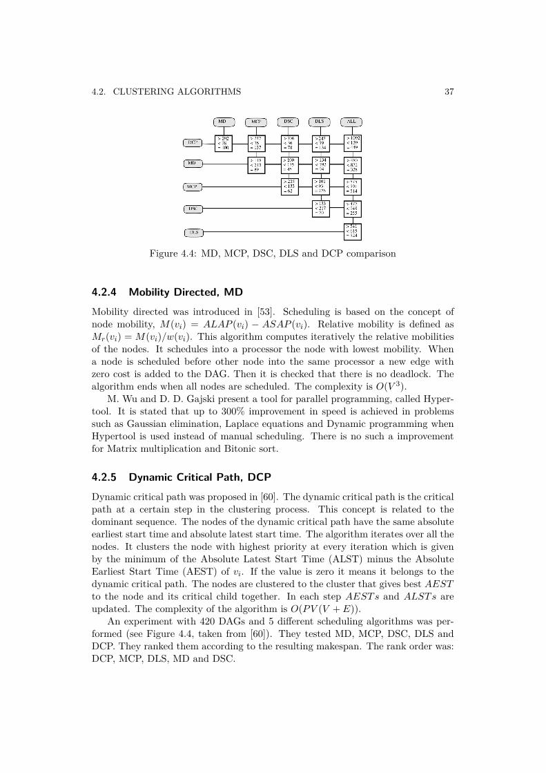
4.2. CLUSTERING ALGORITHMS 37
Figure 4.4: MD, MCP, DSC, DLS and DCP comparison
4.2.4 Mobility Directed, MD
Mobility directed was introduced in [53]. Scheduling is based on the concept ofnode mobility, M(vi) = ALAP (vi) − ASAP (vi). Relative mobility is defined asMr(vi) = M(vi)/w(vi). This algorithm computes iteratively the relative mobilitiesof the nodes. It schedules into a processor the node with lowest mobility. Whena node is scheduled before other node into the same processor a new edge withzero cost is added to the DAG. Then it is checked that there is no deadlock. Thealgorithm ends when all nodes are scheduled. The complexity is O(V 3).
M. Wu and D. D. Gajski present a tool for parallel programming, called Hyper-tool. It is stated that up to 300% improvement in speed is achieved in problemssuch as Gaussian elimination, Laplace equations and Dynamic programming whenHypertool is used instead of manual scheduling. There is no such a improvementfor Matrix multiplication and Bitonic sort.
4.2.5 Dynamic Critical Path, DCP
Dynamic critical path was proposed in [60]. The dynamic critical path is the criticalpath at a certain step in the clustering process. This concept is related to thedominant sequence. The nodes of the dynamic critical path have the same absoluteearliest start time and absolute latest start time. The algorithm iterates over all thenodes. It clusters the node with highest priority at every iteration which is givenby the minimum of the Absolute Latest Start Time (ALST) minus the AbsoluteEarliest Start Time (AEST) of vi. If the value is zero it means it belongs to thedynamic critical path. The nodes are clustered to the cluster that gives best AESTto the node and its critical child together. In each step AESTs and ALSTs areupdated. The complexity of the algorithm is O(PV (V + E)).
An experiment with 420 DAGs and 5 different scheduling algorithms was per-formed (see Figure 4.4, taken from [60]). They tested MD, MCP, DSC, DLS andDCP. They ranked them according to the resulting makespan. The rank order was:DCP, MCP, DLS, MD and DSC.
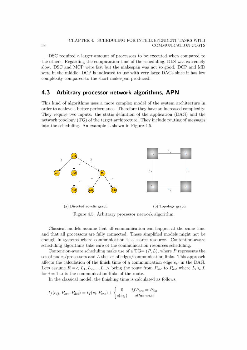
38CHAPTER 4. SCHEDULING FOR INTERDEPENDENT TASKS WITH
COMMUNICATION COSTS
DSC required a larger amount of processors to be executed when compared tothe others. Regarding the computation time of the scheduling, DLS was extremelyslow. DSC and MCP were fast but the makespan was not so good. DCP and MDwere in the middle. DCP is indicated to use with very large DAGs since it has lowcomplexity compared to the short makespan produced.
4.3 Arbitrary processor network algorithms, APNThis kind of algorithms uses a more complex model of the system architecture inorder to achieve a better performance. Therefore they have an increased complexity.They require two inputs: the static definition of the application (DAG) and thenetwork topology (TG) of the target architecture. They include routing of messagesinto the scheduling. An example is shown in Figure 4.5.
(a) Directed acyclic graph (b) Topology graph
Figure 4.5: Arbitrary processor network algorithm
Classical models assume that all communication can happen at the same timeand that all processors are fully connected. These simplified models might not beenough in systems where communication is a scarce resource. Contention-awarescheduling algorithms take care of the communication resources scheduling.
Contention-aware scheduling make use of a TG= (P,L), where P represents theset of nodes/processors and L the set of edges/communication links. This approachaffects the calculation of the finish time of a communication edge eij in the DAG.Lets assume R =< L1, L2, ..., Ll > being the route from Psrc to Pdst where Li ∈ Lfor i = 1...l is the communication links of the route.
In the classical model, the finishing time is calculated as follows.
tf (eij , Psrc, Pdst) = tf (vi, Psrc) +
0 ifPsrc = Pdst
c(eij) otherwise

4.3. ARBITRARY PROCESSOR NETWORK ALGORITHMS, APN 39
In the contention model, the communication edges of the DAG have to be sched-uled in the TG.
tf (eij , Psrc, Pdst) =tf (vi, Psrc) ifPsrc = Pdst
tf (eij , Ll) otherwise
Some arbitrary processor network algorithms will be explained in the following.Parameters from subsection 3.2.2 will be used in order to describe them.
4.3.1 Mapping Heuristic, MH
The mapping heuristic algorithm was presented in [61]. It uses a list-based schedul-ing algorithm that has been modified in order to produce a schedule which is suitablefor a target machine with an arbitrary network topology. It has in mind the effectsof different communication delays depending on the selected route and contentionproblems. Both scheduling and routing are done at every step. A new parametercalled average degree was introduced, AD=number of edges/number of nodes. BothAD and CCR show the weight of the communication in the application.
An ideal model of the network is not good enough in communication intensiveapplications. MH introduces a more advanced model of the communication costs:
c(eij , p1, p2) =(Data(eij)
R+ I
)·H(p1, p2) +D(p1, p2) (4.1)
where the following terms stand for
Data(eij) Amount of sent dataR Speed of the linkI Time to initiate the transmissionH(p1, p2) Number of hops between p1 and p2D(p1, p2) Contention time. Time which the transmission
is delayed due to previously routed transmis-sions.
In the MH algorithm there is a routing table in every processor. The table keepstrack of the communication links usage. It serves to avoid contention problems. Thetable has an entry for each processor of the system. An entry has three data cells.The first one contains the number of hopes to reach the processor. The second onehas the preferred outgoing link to reach the processor. The third one is the delaydue to contention. These tables are used to route the communication edges. Thecomplexity of the algorithm is O(P 3V 2 + PV 2 + P 3), and O(V 2) for a constantnumber of processors.
H. El-Rewini and T. G. Lewis performed simulations with a tool called Task Gra-pher with different network topologies such as ring, star, mesh, hypercube and fullyconnected networks. They proved that in hypercubes the effects of communicationshould be taken into account due to the effect of contention in the communication
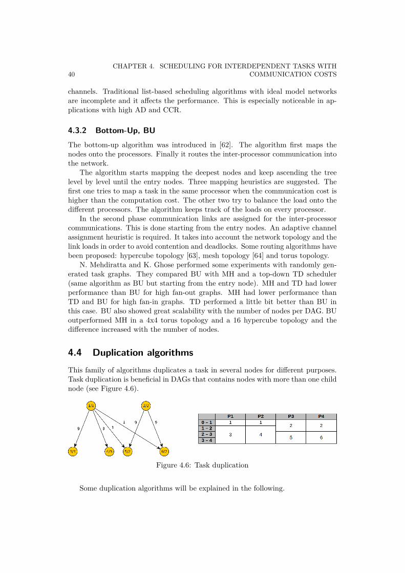
40CHAPTER 4. SCHEDULING FOR INTERDEPENDENT TASKS WITH
COMMUNICATION COSTS
channels. Traditional list-based scheduling algorithms with ideal model networksare incomplete and it affects the performance. This is especially noticeable in ap-plications with high AD and CCR.
4.3.2 Bottom-Up, BU
The bottom-up algorithm was introduced in [62]. The algorithm first maps thenodes onto the processors. Finally it routes the inter-processor communication intothe network.
The algorithm starts mapping the deepest nodes and keep ascending the treelevel by level until the entry nodes. Three mapping heuristics are suggested. Thefirst one tries to map a task in the same processor when the communication cost ishigher than the computation cost. The other two try to balance the load onto thedifferent processors. The algorithm keeps track of the loads on every processor.
In the second phase communication links are assigned for the inter-processorcommunications. This is done starting from the entry nodes. An adaptive channelassignment heuristic is required. It takes into account the network topology and thelink loads in order to avoid contention and deadlocks. Some routing algorithms havebeen proposed: hypercube topology [63], mesh topology [64] and torus topology.
N. Mehdiratta and K. Ghose performed some experiments with randomly gen-erated task graphs. They compared BU with MH and a top-down TD scheduler(same algorithm as BU but starting from the entry node). MH and TD had lowerperformance than BU for high fan-out graphs. MH had lower performance thanTD and BU for high fan-in graphs. TD performed a little bit better than BU inthis case. BU also showed great scalability with the number of nodes per DAG. BUoutperformed MH in a 4x4 torus topology and a 16 hypercube topology and thedifference increased with the number of nodes.
4.4 Duplication algorithmsThis family of algorithms duplicates a task in several nodes for different purposes.Task duplication is beneficial in DAGs that contains nodes with more than one childnode (see Figure 4.6).
Figure 4.6: Task duplication
Some duplication algorithms will be explained in the following.

4.4. DUPLICATION ALGORITHMS 41
4.4.1 Contention-aware scheduling algorithm with task duplication
This algorithm belongs to both the arbitrary processor network family and theduplication family. The purpose of this algorithm is to avoid inter-node commu-nication as much as possible (contention-aware scheduling). This can be done bymeans of task duplication (duplication scheduling). Task duplication increases itsbenefits in a contention-aware context.
There are two different approaches: origin duplication (see Figure 4.7) and des-tination duplication (see Figure 4.8). Both can be combined to improve the perfor-mance.
Figure 4.7: Origin duplication
Figure 4.8: Destination duplication
In [65], the implementation of this algorithm is explained. The algorithm firstfinds the critical parent of a task, the critical parent of the critical parent and soon. The critical parent of a node is the predecessor with highest finish time of thecommunication edge. The next step is to recursively duplicate the critical parentto minimize the finish time, which is done by tentative scheduling and redundanttask/edge removal.
The complexity is O(|P |2|V |2|E|2O(routing)). Where O(routing) is the com-plexity of the routing algorithm.
Contention-aware scheduling with task duplication’s benefits are more noticeablein applications with high amount of communications and networks that are far fromthe ideal case.

42CHAPTER 4. SCHEDULING FOR INTERDEPENDENT TASKS WITH
COMMUNICATION COSTS
4.5 SummaryIn this chapter many algorithms have been presented along with some comparisonsbetween them. Some algorithms get better results than the others but are compu-tationally more complex. Clustering algorithms get reasonably good results at anaffordable complexity.
Arbitrary network processor algorithms and task duplication algorithms shouldbe considered for high performance applications where communication is a bottle-neck.

Chapter 5
Discussion and conclusions forscheduling
This chapter makes use of the knowledge gained in order to provide ideas on howto design and implement a scheduler that fulfills the requirements that were set upin Chapter 1.
5.1 Requirements analysis
An analysis of the requirements list given in Section 1.3 is performed below:
REQ_1 The scheduler shall cope with both serial and parallel applica-tions.The algorithms presented in Chapter 4 are by design able to cope with parallelapplications. A serial application can be seen as a special case of a parallel applica-tion. A serial application is a parallel application with just one task and no edges.Therefore the algorithms presented in Chapter 4 can be easily adapted to cope withserial applications as well.
REQ_2 The scheduler shall do automatic parallelization of the applica-tion. Parallelization shall be transparent to the programmer.Automatic parallelization requires two complex activities. The first one is the de-composition of the application into small tasks with the right granularity. Gran-ularity is a key factor that seriously affects the trade-off between parallelizationand communication. The second activity is to handle the dependencies. A tool forautomatic parallelization has to insert commands in the code for communicationand synchronization of tasks. There is not in the market a tool that completelyabstracts the programmer from this activities. OpenMP is a very popular tool thatwas presented in Chapter 3. In OpenMP the programmer specifies the sections ofcode that can be parallelized by using compiler directives, which is a clean way
43

44 CHAPTER 5. DISCUSSION AND CONCLUSIONS FOR SCHEDULING
since it does not modify the code. The approach of CAP’s compilers is to makea two step decomposition. The first step identifies the hotspots and tries to iso-late them in independent pieces of code, called codelets. The second step is toprofile the application and use machine learning techniques in order to improvethe decomposition. This idea sounds very interesting and has an important benefit.It can adapt to different target platforms thanks to the machine learning techniques.
REQ_3 The scheduler shall parallelize tasks as much as possible.REQ_4 The scheduler shall avoid communication as much as possible.REQ_6 The scheduler shall generate a schedule with the minimum ex-ecution time.Scheduling is a trade-off between parallelization and communication. The optimalschedule finds the right balance. It takes a lot of time to compute the optimalschedule, thus heuristics are used in order to find a solution with a performanceclose to the one of the optimal solution. The algorithms presented in Chapter 4 arenot optimal, they use heuristics. One of the main advantages of the algorithms ofChapter 4 is that if two tasks are mapped to the same processing unit the commu-nication cost is zero. This is true if the output of the predecessor is stored in thelocal memory of the processing unit. In that case the successor retrieves the outputfrom the local memory. It reduces communication and increases performance. Inthe implementation the output of a predecessor shall be stored in local memory.
REQ_5 The scheduler shall provide to an application an end-to-end guar-antee.The DAG is a tool to model parallel applications. This tool can be used to calculateend-to-end latencies in multi-core systems. The makespan of the application is whatgives the end-to-end latency. In real-time systems the end-to-end latency shall besmaller than a deadline.
REQ_7 The scheduler shall be energy efficient.There are two ways of increasing energy efficiency. The first method is by increas-ing parallelization. Two small energy efficient cores can perform the same task asa powerful processor with less energy. The second method is by using the powersaving mechanisms provided by the target platform. The prototype board providesan idle mode to sleep cores if they are not used.
REQ_8 The scheduler shall be target independent. The algorithm shallbe easily portable to other platforms.List-based algorithms, clustering algorithms and duplication-based algorithms donot have dependencies with the platform. It means that the algorithms are easilyportable from a target system to a different target system. However, arbitrary pro-cessor network algorithms are target dependent. These algorithms need an extrainput, the TG. Extra performance is gained in exchange of portability.

5.2. PERFORMANCE COMPARISON 45
5.2 Performance comparisonThere are two basic parameters to measure the performance of the algorithms: thecomplexity and the makespan. The complexity tells how much time is needed toconstruct the schedule. The makespan is the length of the schedule produced.
List-based algorithms are based on very simple ideas or heuristics. However,the makespan and the time to construct the schedule is not very good. Clusteringalgorithms are normally based on list-based algorithms. Their complexity is usuallylower than the one of list-based algorithms and the produced makespan is still good.This is due to the fact that they assume an unlimited number of processors toschedule the tasks. LC is an algorithm that gives optimal solutions for coarse grainin-tree and join/fork DAGs at a low complexity (see table 5.1).
Arbitrary processor network algorithms are recommended to be used in appli-cation with high CCR and where the communication network is far from the idealcase. The complexity of the implementation is greater than in the other algorithmfamilies, specially with complex network topologies. Only the previous conditionsjustify their usage. BSA is the algorithm with better performance among the algo-rithms studied according to [66] (see table 5.2).
Duplication-based algorithms are more complex in order to reduce the makespan.They should be used only in cases where a very short makespan is required.
Novel algorithms combined the ideas from arbitrary processor network andduplication-based algorithms [65]. It turns out that there is a synergy betweenthe ideas and quite good results are obtained.

Source List-based ClusteringHLFET MCP ETF DLS EZ LC DSC MD DCP
[1] Makespan Longest Medium-long Medium-short Shortest N/A N/A N/A N/A N/AComplexity O(PV 2) O(PV 2) O(PV 3) O(PV 3) N/A N/A N/A N/A N/A
[59] Makespan N/A Optimal in-tree Optimal in-tree N/A N/A Optimal in-tree/join-fork
Optimal join-fork N/A N/A
Complexity N/A O(V 2 log V ) O(PV 2) N/A N/A O((V + E) log V ) O(PV (V + E)) N/A N/A
Table 5.1: List-based algorithms and clustering algorithms: Performance comparison
Source Arbitrary processor network Reduction of makespan by using BSA
[65]MH 40%DLS 50%BU 71%
Table 5.2: Arbitrary processor network: Performance comparison

5.3. DESIGN DECISIONS 47
5.3 Design decisions
The aim of this thesis is to implement a code generation toolchain for parallelapplications. In this section the design decisions to fulfill the requirements will belisted. The implementation process will be iterative.
The aim is to use a simple algorithm first in order to get to know the hardware.A simple algorithm is also simpler to debug. Once the first prototype is workingnew features will be implemented.
The first algorithm to be implemented is linear clustering. In table 5.3 the mainfeatures of the toolchain are listed and mapped with the requirements they meet.REQ_2 is only partially fulfilled because the dependencies are handled but thedecomposition has to be done manually by the programmer.
Item Description Fulfilledrequirements
Implementation ofLC on the prototypeboard
LC provides optimum schedules foroptimal coarse grain in-tree andjoin/fork DAGs. The algorithm is alsoindependent from the target platform.
REQ_3,REQ_4,REQ_6 andREQ_8
Adaptation for serialapplications
REQ_1
Utilization of thetarget energy modes
Energy modes will sleep the coreswhen not being used.
REQ_7
Implementation of aDAG generator
The output DAG from the generatorwill be the input to the scheduler.The DAG is drawn by theprogrammer in a GUI.
REQ_2(partially)
Offline calculation ofthe makespan
The calculation will serve as anend-to-end latency guarantee.
REQ_5
Table 5.3: First prototype specification
A new prototype will be implemented once the first prototype works correctly.There is room for improvement changing the scheduling algorithm. A duplicationbased algorithm could reduce the makespan. The algorithm would duplicate taskswith more than one successor.
The ideal system would be an arbitrary processor network algorithm with taskduplication (see table 5.4). The Epiphany network-on-chip would be taken intoaccount in order to avoid communication contention due to the side-effects of inter-task communication. Something important to notice is that this prototype wouldnot meet REQ_8. This is accepted because the previous prototype met REQ_8.The programmer would implement the application as a serial application and thetoolchain would identify the optimal decomposition of the application into tasks

48 CHAPTER 5. DISCUSSION AND CONCLUSIONS FOR SCHEDULING
and would handle their scheduling and dependencies. No graph would be neededto draw. One possibility to be considered is that the final system would run severalalgorithms and select the one with the best performance.
Item Description Fulfilledrequirements
Customizedscheduler for theprototype board
Arbitrary processor network + taskduplication algorithm
REQ_3,REQ_4 andREQ_6
Adaptation for serialapplications
REQ_1
Utilization of thetarget energy modes
Energy modes will sleep the coreswhen not being used.
REQ_7
Implementation of aDAG generator
The output DAG from the generatorwill be the input to the scheduler.The DAG is generated from the serialversion of the application.
REQ_2
Offline calculation ofthe makespan
The calculation will serve as anend-to-end latency guarantee.
REQ_5
Table 5.4: Ideal system specification

Part II
Practical phase
49


Chapter 6
System design and architecture:Toolchain
The system to be implemented has been thought as a toolchain. The main use caseof the system consists in giving a graph representing a parallel application as theinput and getting some files with the skeleton of the application as the output. Anode is a part of code that cannot run in parallel but sequentially on a specific core.Figure 6.1 shows the toolchain modules and how they are connected together. Italso shows the outputs of each module, which are the inputs to the next module.
Figure 6.1: Toolchain
6.1 Graph editor
The graph editor used is yEd. It is a freeware software that runs on Windows, Linuxand Mac OS. The program is able to load and save diagrams from/to XML-basedformat files.
Figure 6.2 shows an example of a graph drawn in yEd. It has 6 nodes and 7edges. Each node contains the node id and the node weight separated by the slashcharacter. Each edge has the communication cost.
51

52 CHAPTER 6. SYSTEM DESIGN AND ARCHITECTURE: TOOLCHAIN
Figure 6.2: yEd graph
Figure 6.3: Node and edge structures
6.2 Xgml parser moduleThe xgml parser initializes the DAG. It reads the xgml file generated by the grapheditor and generates two linked lists: a node list and an edge list (see Figure 6.3).
The module uses libxml2, which is a software library written in C for parsingXML documents. It was developed for the GNOME project and is available underthe MIT License.
A node is a structure with a graph id, an id, a weight, a top level, a bottom leveland a pointer to the next node in the linked list. The graph id is a field defined bythe graph editor and that is required to identify the edges that link nodes. The idis a number given by the user. The weight is the execution time of the task. Thetop level and the bottom level are two fields used by the linear clustering algorithm.
An edge is a structure with a predecessor, a successor, a cost and a pointer tothe next edge in the linked list. The predecessor is the source node where the edgestarts from. The successor is the sink node where the edge is pointing at. The costis the communication time.

6.3. CLUSTERING ALGORITHM MODULE 53
6.3 Clustering algorithm moduleThe clustering algorithm module implements linear clustering, proposed by [58].Many algorithms are described in [46], among them linear clustering. Its descriptionis presented below.
Algorithm 1 Linear clusteringEunex: set of unexamined edgesVunex: set of nodes v ∈ V on which edges Eunex are incidentCreate initial clustering C0: allocate each node v ∈ V to a distinct cluster C ∈ C|C| = |V|Eunex ← Ewhile Eunex 6= ∅ doFind a critical path cp of graph Gunex = (Vunex,Eunex)Merge all nodes Vcp of cp into one clusterEunex ← Eunex − eij ∈ Eunex : vi ∈ Vcp ∨ vj ∈ Vcp
end while
In order to find the critical path of the DAG, the top level and the bottom level ofeach node are calculated. To do that it is necessary to sort the nodes topologically.The implementation uses the algorithm proposed by [67]. The complexity of thealgorithm is O(|V |+ |E|).
Algorithm 2 Topological sortingL← Empty list that will contain the sorted elementsS← Set of all nodes with no incoming edgeswhile S 6= ∅ doRemove a node v from SInsert v into Lfor all node m with an edge e from v to m doRemove edge e from the graphif m has no other incoming edges thenInsert m into S
end ifend forif graph has edges thenReturn error (graph has at least one cycle)
elseReturn L (a topologically sorted order)
end ifend while
The output of this module is a linked list per cluster and a list with the headnodes of the clusters. Each cluster contains a list of tasks that will be mapped to a

54 CHAPTER 6. SYSTEM DESIGN AND ARCHITECTURE: TOOLCHAIN
Figure 6.4: Generated code
specific core.
6.4 Code generator moduleThe code generator module is in charged of generating the skeleton code of theapplication. Once it is generated, it has to be loaded onto the Epiphany projects.
Figure 6.4 shows the generated code for the brake-by-wire application. It iscreated in a folder called generated_code. Inside generated_code there are threekinds of folders: common, core_i and host. The application shown in the figurerequires 6 cores for the execution.
The code in folder common goes to a common project for all the cores. It con-tains the software modules that allow us to run the parallel application on Epiphany.The core_i folder contains specific code for a core, mainly the tasks that the corehas to execute. The host folder is the generated code that the host computer hasto run to start Epiphany and fetch the results once Epiphany has finished.

6.5. APPLICATION DEVELOPMENT 55
6.5 Application developmentAfter the skeleton code has been generated, the user has to define the followingsections.
• The inputs of the parallel application.
• The outputs of the parallel application.
• The calculations section of the tasks.
• The communication edges between tasks.
The inputs and the outputs are empty structures. Inside the structures theprogrammer creates the fields for the specific application.
1 typedef struct 23 input_i_t ;45 typedef struct 67 output_j_t ;
Below it is presented an example of the code generated for a task. The sectionsinside a task are always the same: input, output, retrieve the input, start task profiler,calculations, end task profiler and transmit results. All sections are generated bythe code generator module except the calculations section that is specific of theapplication.
1 void task_j (void )2 3 // Input4 edge_ij_t edge_i j ;56 // Output7 edge_jk_t edge_jk ;89 // Ret r i eve the input
10 while (0 != retr i eve_message ( i , j , &edge_i j ) )11 __asm__( "IDLE ; " ) ;1213 s t a r t_ta sk_pro f i l e r ( ) ;1415 // Do c a l c u l a t i o n s and s t o r e the r e s u l t s16 // input = f ( output ) ;

56 CHAPTER 6. SYSTEM DESIGN AND ARCHITECTURE: TOOLCHAIN
17 //18 // User code1920 Log_tasks_core [ j ] = end_task_pro f i l e r ( ) ;2122 // Transmit the r e s u l t s23 send_message ( s izeof ( edge_jk_t ) , j , k , &edge_jk ,
CORE_NUMBER_k) ;24 return ;25
The last step is to define the communication edges, which are also empty struc-tures where the user creates customized fields.
1 typedef struct 23 edge_ij_t , ∗pointer_edge_ij_t ;

Chapter 7
System design and architecture:Epiphany application
In this chapter it will be described the software modules that allow us to run aparallel application on Epiphany. The system is made up of six software modules:epiphany module, file system module, interrupts module, mailbox module, host com-munication module and profiler module. Figure 7.1 shows the stack diagram of thesystem.
Figure 7.1: Software modules stack
Some software modules requires the definition of a set of data structures in thelocal memory. The location of these data structures is specified in a linker definitionfile. That file also tells the compiler to place the stack in the local memory instead ofthe external DRAM and to place the Interrupt Vector Table (IVT) at the beginningof the local memory. Figure 7.2 shows how the local memory of a core and the sharedmemory of the board are used.
7.1 Epiphany moduleThis module defines a global variable called Me. Me contains relevant informationabout the core that is used by other modules, see Table 7.1.
57

58CHAPTER 7. SYSTEM DESIGN AND ARCHITECTURE: EPIPHANY
APPLICATION
Figure 7.2: Board memory
7.2 Interrupts module
The interrupts module is where the ISRs of the system are declared and defined.An ISR is a callback function which is triggered by an interrupt. An interrupt is asignal to the processor indicating the arrival of a new event. There are two kinds ofinterrupts depending on the nature of the event: hardware interrupts and softwareinterrupts.
Hardware interrupt: is generated by either an internal peripheral or an ex-ternal peripheral to the processor. The hardware interrupts in epiphany are: syn-chronization/reset, timer 0 expired, timer 1 expired, Direct Memory Access (DMA)channel 0 end of transfer and DMA channel 1 end of transfer.
Software interrupt: is generated by an exceptional condition or a specialinstruction. The software interrupts in epiphany are: software exception, memoryprotection fault and software interrupt.
Each core has an interrupt controller that is in charged of executing the appro-priate ISR depending on the interrupt generated. Figure 7.3, taken from [68], showsthe operation workflow. ILAT is a system register that records all interrupt events.IMASK is a system register for blocking interrupts. IPEND is a system register
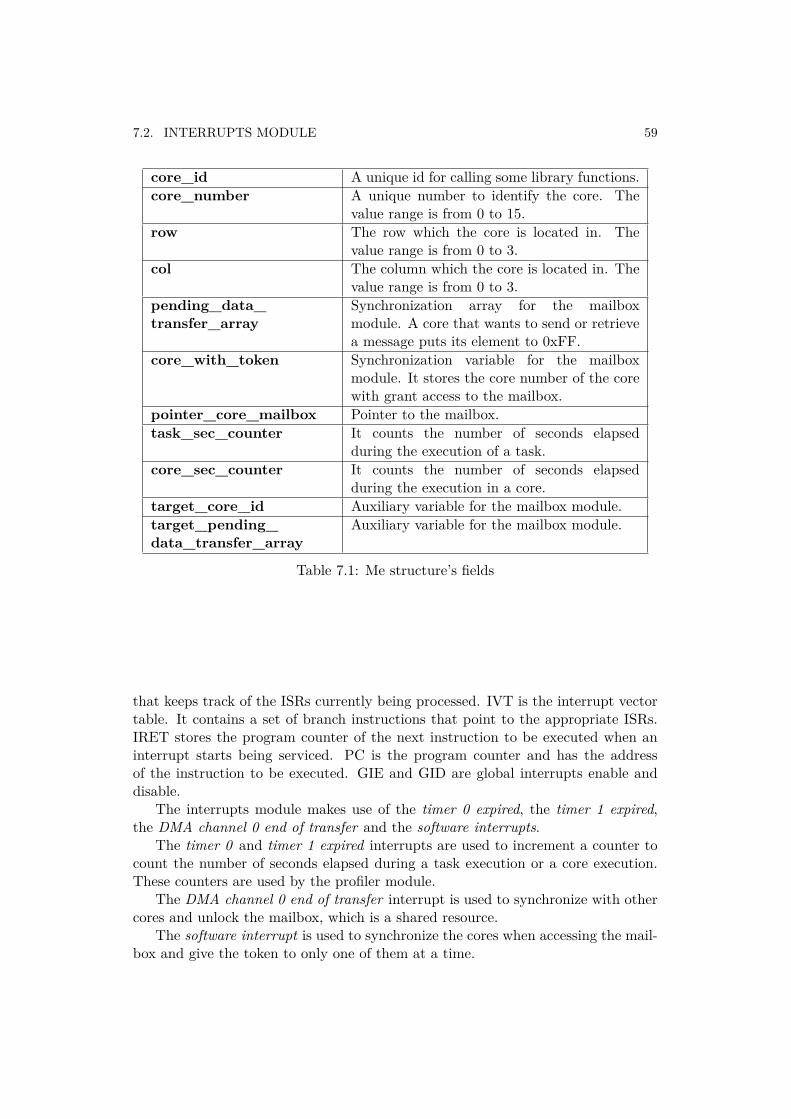
7.2. INTERRUPTS MODULE 59
core_id A unique id for calling some library functions.core_number A unique number to identify the core. The
value range is from 0 to 15.row The row which the core is located in. The
value range is from 0 to 3.col The column which the core is located in. The
value range is from 0 to 3.pending_data_transfer_array
Synchronization array for the mailboxmodule. A core that wants to send or retrievea message puts its element to 0xFF.
core_with_token Synchronization variable for the mailboxmodule. It stores the core number of the corewith grant access to the mailbox.
pointer_core_mailbox Pointer to the mailbox.task_sec_counter It counts the number of seconds elapsed
during the execution of a task.core_sec_counter It counts the number of seconds elapsed
during the execution in a core.target_core_id Auxiliary variable for the mailbox module.target_pending_data_transfer_array
Auxiliary variable for the mailbox module.
Table 7.1: Me structure’s fields
that keeps track of the ISRs currently being processed. IVT is the interrupt vectortable. It contains a set of branch instructions that point to the appropriate ISRs.IRET stores the program counter of the next instruction to be executed when aninterrupt starts being serviced. PC is the program counter and has the addressof the instruction to be executed. GIE and GID are global interrupts enable anddisable.
The interrupts module makes use of the timer 0 expired, the timer 1 expired,the DMA channel 0 end of transfer and the software interrupts.
The timer 0 and timer 1 expired interrupts are used to increment a counter tocount the number of seconds elapsed during a task execution or a core execution.These counters are used by the profiler module.
The DMA channel 0 end of transfer interrupt is used to synchronize with othercores and unlock the mailbox, which is a shared resource.
The software interrupt is used to synchronize the cores when accessing the mail-box and give the token to only one of them at a time.
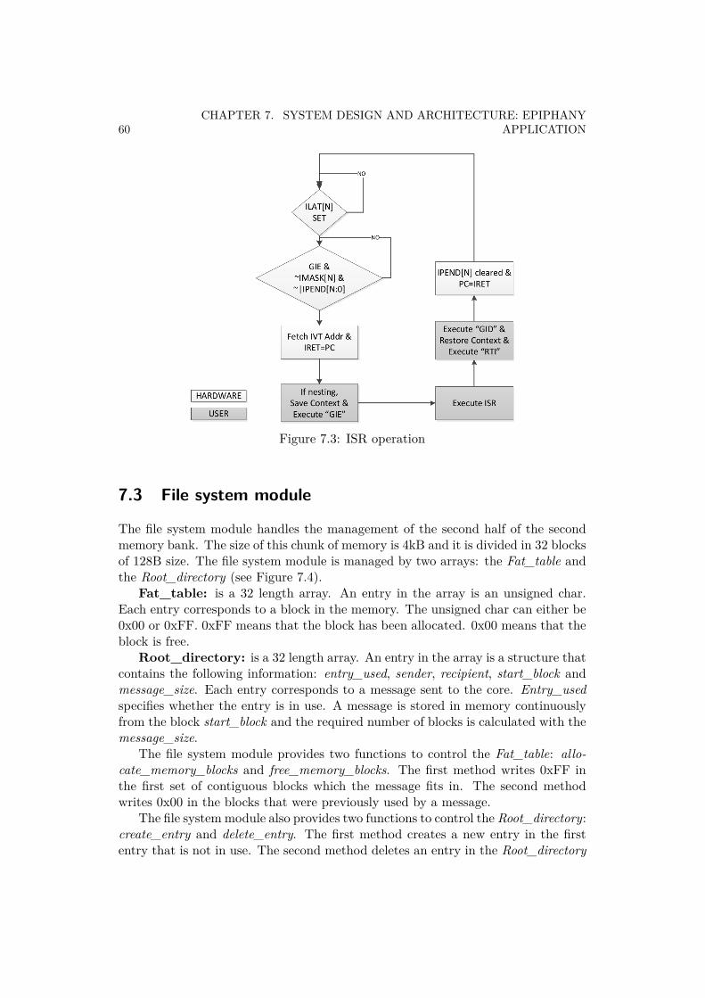
60CHAPTER 7. SYSTEM DESIGN AND ARCHITECTURE: EPIPHANY
APPLICATION
Figure 7.3: ISR operation
7.3 File system module
The file system module handles the management of the second half of the secondmemory bank. The size of this chunk of memory is 4kB and it is divided in 32 blocksof 128B size. The file system module is managed by two arrays: the Fat_table andthe Root_directory (see Figure 7.4).
Fat_table: is a 32 length array. An entry in the array is an unsigned char.Each entry corresponds to a block in the memory. The unsigned char can either be0x00 or 0xFF. 0xFF means that the block has been allocated. 0x00 means that theblock is free.
Root_directory: is a 32 length array. An entry in the array is a structure thatcontains the following information: entry_used, sender, recipient, start_block andmessage_size. Each entry corresponds to a message sent to the core. Entry_usedspecifies whether the entry is in use. A message is stored in memory continuouslyfrom the block start_block and the required number of blocks is calculated with themessage_size.
The file system module provides two functions to control the Fat_table: allo-cate_memory_blocks and free_memory_blocks. The first method writes 0xFF inthe first set of contiguous blocks which the message fits in. The second methodwrites 0x00 in the blocks that were previously used by a message.
The file system module also provides two functions to control the Root_directory:create_entry and delete_entry. The first method creates a new entry in the firstentry that is not in use. The second method deletes an entry in the Root_directory

7.4. MAILBOX MODULE 61
Figure 7.4: Fat_table and the Root_directory
by putting the field entry_used into not in use.
7.4 Mailbox module
The mailbox module provides a system service to send and receive inter-core mes-sages. This communication service has a high level of abstraction. Beneath it usesthe interrupts module and the file system module. It implements two functions:send_message and retrieve_message.
The mailbox system stores the messages in the memory space managed by thefile system module. It is a 4kB memory area located at address 0x5000. All the coreshave access to the mailbox of a specific core. This fact makes it a shared resource.Therefore special precautions have to be taken. A synchronization mechanism needsto be implemented. The synchronization mechanism designed is made up of twovariables in each core: pending_data_transfer_array and core_with_token.
pending_data_transfer_array: is an sixteen-size array. The first elementof the array corresponds to the first core, the second element to the second core andso on. When a core wants to send or retrieve a message from another core, it hasto write 0xFF into its element. Once the operation has been completed the corewrites 0x00 back into the element.
core_with_token: contains the number of the core with grant access to sendor retrieve messages. The value of this variable is re-evaluated every time there isa software interrupt.
The function send_message is used to transfer a message into a specific core.Figure 7.5 shows a description of the send_message function.

62CHAPTER 7. SYSTEM DESIGN AND ARCHITECTURE: EPIPHANY
APPLICATION
Figure 7.5: Send_message function
Figure 7.6: Retrieve_message function
The function retrieve_message is used to retrieve a message from the mailbox.Figure 7.6 shows a description of the retrieve_message function.
7.5 Host communication module
The host communication module is the place where the programmer defines theinputs and the outputs of the parallel application.
The module defines the variable Mailbox_host_epiphany in external DRAM(address 0x81000000), which contains the inputs, the outputs, the input flag andthe output flags.
The flags are variables to synchronize the cores with the host. The cores do notstart the execution until the input flag is set to 1. The host do not fetch the resultsuntil all the output flags are set to 1.

7.6. PROFILER MODULE 63
Figure 7.7: Profiler functions
7.6 Profiler moduleThe profiler module measures the execution time of the cores and the executiontime of the tasks (see Figure 7.7). The measurements are stored in a log.
A core has two available timers: timer 0 and timer 1. A timer has a 32-bit reg-ister to count and the frequency of the clock is 600Mhz. Both timers are configuredto generate an interrupt every second. The interrupts increment a counter.
Timer 1 is used to profile a core. Start_core_profiler is a function that resetsthe counter and starts the timer. It is called just after the input flag is set to 1.After the core has executed all task assigned to it, the timer value is recorded inthe log with the function record_core_time. The value of the timer is given in clockticks. Therefore it has to be scaled to nanosecond when storing it into the log.
Timer 0 is used to profile the tasks in a core. Start_task_profiler function resetsthe counter and starts the timer. Record_task_time records its value.
Two arrays are allocated in external DRAM. Log_cores_ram (address 0x81001000)stores the cores’ execution time. 8 bytes are needed for each of the 16 cores.Log_tasks_ram (address 0x81001000) stores the tasks’ execution times. Writinginto the external RAM adds extra traffic into the e-mesh, therefore the tasks’ execu-tion times are first stored into Log_tasks_core (address 0x6160) located in internalRAM and after moved to Log_cores_ram.


Chapter 8
Implementation
This chapter provides the decisions taken during the implementation phase that arenot covered in Chapters 6 or 7.
8.1 Power managementThe Epiphany chip provides the IDLE instruction to put a core into a low-power orstandby state. After a reset a core is in idle. An external interrupt event activatesthe core. The core keeps active until an IDLE instruction. The core returns to thenormal execution after another interrupt event.
Every core has a 32-bit STATUS register that contains information regardingthe execution status. Bit 0 is a flag called ACTIVE. 0 indicates that the core is idleand 1 indicates that the core is active. When the core is in the standby state, theclocks are disabled and the power consumption is minimized.
This mode is used when retrieving messages from the mailbox. If the messagehas not arrived by the time it has been tried to be retrieved, the core is deactivated.The actual implementation is shown below.
1 // Ret r i eve the input2 while (0 != retr i eve_message ( i , j , &edge_i j ) )3 __asm__( "IDLE ; " ) ;
The core is woken up when another core sends a message to him. First thesender raises a remote interrupt to get the token. The recipient goes to the idlemode again since the transfer is not completed yet. Once the transfer is completedthe sender raise another remote interrupt to the recipient. This time the messageis in the mailbox and the core can resume the execution.
1 // Send i n t e r r u p t to r e c i p i e n t2 e_irq_remote_raise ( coreID , (E_SW_INT + SOFF) ) ;34 // Wait u n t i l the token i s go t
65

66 CHAPTER 8. IMPLEMENTATION
5 while (Me. core_number != ∗ target_core_with_token )6 __asm__( "IDLE ; " ) ;78 // Copy the data to the d e s t i n a t i o n9
10 // Send i n t e r r u p t to r e c i p i e n t a f t e r the t r an s f e r11 e_irq_remote_raise ( coreID , (E_SW_INT + SOFF) )
8.2 Inter-core communicationEach core is equipped with a DMA engine. Its function is to offload a core fromdata movement. It is capable of a double word transaction on every clock cycle ata 600Mhz frequency, which means a sustained data transfer rate of 8 GB/sec.
A high level of abstraction schematic for the epiphany chip is given in Figure8.1, taken from [68].
Figure 8.1: Epiphany schematic
The engine has two independent channels, channel 0 and channel 1. Channel 0is used for sending and retrieving messages, while channel 1 stays unused. It hasbeen configured as a master and it generates an event interrupt when the transferfinishes. A data movement does not start until a previous data movement completesand the channel is free.

8.2. INTER-CORE COMMUNICATION 67
The configuration of the DMA to send or retrieve a message is shown below.
1 // Copy the data2 e_tcb_t usr_tcb ;3 usr_tcb . c on f i g = E_DMA_ENABLE | E_DMA_MASTER | E_DMA_IRQEN
| E_DMA_BYTE;4 usr_tcb . i nne r_s t r i d e = 0x00010001 ;5 usr_tcb . count = 0x10000 | s i z e ;6 usr_tcb . oute r_s t r ide = 0x00000000 ;7 usr_tcb . src_addr = source ;8 usr_tcb . dst_addr = de s t i n a t i on ;9 e_dma_start (E_DMA_0, &usr_tcb ) ;

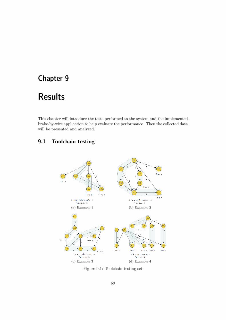
Chapter 9
Results
This chapter will introduce the tests performed to the system and the implementedbrake-by-wire application to help evaluate the performance. Then the collected datawill be presented and analyzed.
9.1 Toolchain testing
(a) Example 1 (b) Example 2
(c) Example 3 (d) Example 4
Figure 9.1: Toolchain testing set
69

70 CHAPTER 9. RESULTS
The toolchain testing procedure has consisted in introducing representative DAGsinto the toolchain. The results have been compared with the expected result inorder to verify the system (see Figure 9.1).
The first example is a 6-node DAG. The toolchain divides it into three clusters.It also calculates the critical path length and the makespan, 17 and 16 respectively.There are some interesting aspects. For instance, node 1 forks into four brancheswhereas two branches join into node 5. It can also be highlighted that there is morethan one exit node, three in this case.
Example 2 is rather similar to example 1 but with a higher degree of complexity.The critical path length and the makespan are 25 and 21. Example 3 is more specialbecause there is more than one entry node, two in this case. The critical path lengthand the makespan are 29 and 25.
Example 4 is the one used for the brake-by-wire application. The DAG containsthree entry nodes and five exit nodes (one for the traction motor and four thebrake motors at the wheels). The critical path length and the makespan are 17 and17. In this case the makespan is not shorter than the critical path length. Linearclustering does not obtain an optimal solution. There exist other solutions thatoutperform the one obtained by the toolchain. The solution presented in Figure 9.2has a makespan of 16, one time unit less.
Figure 9.2: Alternative DAG with shorter makespan
The toolchain has been evaluated with 12 DAGs in total. Four representativeexamples have been shown in this section. In each example different aspects wereevaluated. The covered aspects are join nodes, fork nodes, entry nodes, exit nodes,different tasks weights and different communication costs. A summary of the eval-uated aspects is presented in Table 9.1. The last column of the table correspondsto the other 8 DAGs that are not presented in this report.

9.2. BRAKE BY WIRE APPLICATION 71
Ex. 1 Ex. 2 Ex. 3 Ex. 4 Rest of DAGsJoin nodes 3 3 3 3 3
Fork nodes 3 3 3 3 3
More than oneentry node
7 7 3 3 3
More than oneexit node
3 3 7 3 3
Different weights 7 3 3 7 3
Different costs 7 7 7 7 3
Table 9.1: Summary of the evaluated aspects with each example DAG
9.2 Brake by wire application
Figure 9.3: Brake-by-wire physical view
A brake-by-wire application has been implemented for the final demonstrationplatform. The application runs on the Epiphany E16 development board. Thesystem’s physical view is presented in Figure 9.3. It is made up of the followingphysical components.
• A brake pedal sensor and a throttle pedal sensor.
• A main motor and its controller.
• A brake motor and its controller.
• Four Arduino boards.

72 CHAPTER 9. RESULTS
Figure 9.4: Brake-by-wire epiphany application
• Four Raspberry Pi.
• A desktop computer.
• A Epiphany E16 development board.
The inputs of the parallel application are the required brake torque, the requiredthrottle torque and the wheel speeds in rpm. The inputs are obtained from the threesensors: the two pedal sensors and the hall sensors from the main motor. A pedalsensor consist of a potentiometer. The voltage value is read by a Arduino boardand processed to get a percentage value. The motor controller has been configuredto have an output whose voltage is proportional to the main motor speed. Thevoltage value is read by another Arduino board and processed to get a percentagevalue (100% represents 3400 rpm). The speed of the other three wheels is simulatedwith a random function.
Figure 9.4 shows a graph of the brake-by-wire application. The code for theEpiphany E16 development board is generated automatically by the toolchain. Thecalculation’s part of each task has to be fill in by the programmer. The code used inthe test is attached in Appendix C. A short description of the tasks is given below.
• Task 1: transforms the throttle percentage value to the real value.
• Task 2: calculates the electrical signal for the main motor.
• Task 3: transforms the brake percentage value to the real value.
• Task 4: calculates the speed of the car (average speed of the four wheels).
• Task 5, 6, 7 and 8: calculates the slip value of one wheel.

9.2. BRAKE BY WIRE APPLICATION 73
Figure 9.5: Brake-by-wire host application
• Task 9, 10, 11 and 12: calculates the electrical signal for the brake motorof one wheel.
Both the execution time of the tasks and the communication time between themare unknown. Therefore it is assumed that all the tasks have the same executiontime, 5 time units. The second assumption is that the communication time is alwaysthe same, 1 time unit.
On the host computer there is other deployed program (see Figure 9.5). Thisprogram has three monitor variables protected by pthread mutexes: Input_data,Output_data and Log_data. There are also three threads: epiphany_host_thread,mosquitto_client_thread and linx_peer_thread. The mosquitto_client_thread isin charged of updating the Input_data with the information published by theMosquitto server, which runs on the main Raspberry Pi node. The epiphany_host_thread is in charged of starting the execution of epiphany and updating the Out-put_data and Log_data when the execution has completed. The linx_peer_threadsends the Output_data and Log_data to the trace server, which runs on the mainRaspberry Pi node.

74 CHAPTER 9. RESULTS
9.3 Collected data
9.3.1 Power consumption’s dataThe Epiphany chip is equipped with a current sense resistor. The value of theresistor is 0.02Ω. The sense gain of the system is 50. Therefore, the voltage measuredon the measurement point Vcore(A) is equal to the core current. The voltage supplyfor Epiphany is Vcore, 1089mV. The power consumption is given by the followingexpression.
PEpiphany = Vcore · Icore
= Vcore · Vcore(A) = 1.089 · Vcore(A)
Figure 9.6 shows the power consumption in Epiphany as a function of the idlecores. The power consumption when all the cores are in idle is 382.239mW. Thepower saving when idling a core is between 21.79mW and 22.869mW. It means a5.98% of the static consumption per core and about a 98% with all the cores. Theprogram used to test Epiphany is attached in Appendix A.
Figure 9.6: Epiphany power consumption
9.3.2 Timers’ dataThe profiler module has to kind of functions: start_core_profiler/start_task_profilerand record_core_time/record_task_time. A core is using timer 1 to profile and atask is using timer 0 to profile.
Some tests have been performed to measure the accuracy of the profiling system.In the first test the time when no operation is performed is measured. time_1 is101ns.
1 s t a r t_co r e_p ro f i l e r ( ) ;

9.3. COLLECTED DATA 75
2 log_t time_1 = record_core_time ( ) ;
The next test starts the other timer. time_1 is 245ns. Therefore the timenecessary for executing start_task_profiler is 144ns (101ns subtracted).
1 s t a r t_co r e_p ro f i l e r ( ) ;2 s t a r t_ta sk_pro f i l e r ( ) ;3 log_t time_1 = record_core_time ( ) ;
The next test starts the task timer and record a time. time_1 is 105ns andtime_2 is 6008ns (if task and core functions are inverted the result is 100ns and5986ns). Therefore the time to start a timer and record a value is 5907ns (101ns sub-tracted). Then 144ns are subtracted for start_task_profiler, 5763ns. The countercounted 105ns. It means that the timer did not start until 5658ns (105ns sub-tracted).
1 s t a r t_co r e_p ro f i l e r ( ) ;2 s t a r t_ta sk_pro f i l e r ( ) ;3 log_t time_1 = record_task_time ( ) ;4 log_t time_2 = record_core_time ( ) ;
The last test consists of recording the task time twice. time_1 is 105ns, time_2is 5870ns and time_3 is 11658ns. Therefore record_task_time takes 5788ns. Thisseems to be correct since 5788ns is very close to 5658ns plus 105ns (5763ns).
1 s t a r t_co r e_p ro f i l e r ( ) ;2 s t a r t_ta sk_pro f i l e r ( ) ;3 log_t time_1 = record_task_time ( ) ;4 log_t time_2 = record_task_time ( ) ;5 log_t time_3 = record_core_time ( ) ;
The times can be summarized as follows:
• start_task_profiler: 144ns.
• timer start time after start_task_profiler: 5658ns.
• record_task_time: 5788ns.
9.3.3 Single core application’s dataIn order to evaluate the performance of the parallel application it is necessary tocollect data of an equivalent serial application (see Figure 9.7). The code is attachedin Appendix B.

76 CHAPTER 9. RESULTS
Figure 9.7: Brake-by-wire application (single core)
Both core profiler and task profiler are used at the same time. The task profileronly measures the time for the calculations whereas the core profiler measures thetime to fetch the input, send the output and put the output_flag to 1 as well.The measurement of the core profiler is affected by the task profiler measurement.Therefore another experiment is performed without the task profiler. The result isaround 6000ns less, see 9.2.
Task profiler Core profiler Core prof. aloneMean time [ns] 13368 22627 16623
Table 9.2: Single core application’s task and core profiler
Other experiments are performed in order to identify where the other 3000nsare spent. The results are shown in Table 9.3.
Mean time [ns]Before fetching input data 123After fetching input data 3128Before sending output data 16529After sending output data 16602After setting output flag to 1 16623
Table 9.3: Single core application’s timing
The times can be summarized as follows:
• Calculations: 13368ns.

9.3. COLLECTED DATA 77
• Application: 16623ns.
• Fetching input data: 3105ns.
• Sending output data: 73ns.
• Setting output flag to 1: 21ns.
The energy consumption is:
Energy =(Poweridle
16 + Power1core
)· time
=(382mW
16 + 22mW)· 16623ns = 0.762µJ
9.3.4 Parallel application’s data
The execution times of the cores are shown in Table 9.4.
Core 0 Core 1 Core 2 Core 3 Core 4 Core 5Mean time [ns] 35126 45399 24182 55508 52824 60908
Table 9.4: Parallel application’s core profiler
The total execution time of the application is 60908ns. The energy consumptionof the application is calculated as follows.
Energy =∑(
Poweridle
16 + Power1core
)· timecorei
=∑(382mW
16 + 22mW)· timecorei
= 12.567µJ
When the idle capability is included in the code, the energy consumption isdecreased. The cores get into the idle mode because they are blocked waiting for amessage. There is an option in the timers to count the number of idle cycles. Theresults are shown in Table 9.5.
Core 0 Core 1 Core 2 Core 3 Core 4 Core 5Idle time [ns] 7589 2906 6141 12233 15403 26042
Table 9.5: Number of idle cycles

78 CHAPTER 9. RESULTS
The idle time needs to be included in the calculations of the energy consumption.The following equation is used.
Energy =∑ Poweridle
16 · timecorei + Power1core · (timecorei − idle_timecorei)
=∑ 382mW
16 · timecorei + 22mW · (timecorei − idle_timecorei)
= 11.020µJ
Figure 9.8: Brake-by-wire application timing
Figure 9.8 shows the timing of the parallel application measured with the timers.The colored edges represent inter-core communication and make use of the mailboxsystem. At the departing point there are two rows. The first row contains thesystem time in microseconds before sending the message. The second row containsthe system time after sending the message. At the arrival point there are anothertwo rows. The first row contains the system time at which the core first tries toretrieve the message. The second row contains the system time after retrieving themessage. Sometimes the measured value is not constant, then the minimum andmaximum measured value are put instead.
Table 9.6 shows the time elapsed in each task.

9.3. COLLECTED DATA 79
Mean time [ns]Task 1 350Task 2 190Task 3 373Task 4 2853Task 5 2301Task 6 2301Task 7 2301Task 8 2308Task 9 990Task 10 988Task 11 988Task 12 988
Table 9.6: Parallel application’s task profiler
9.3.5 Parallel application with task duplication’s data
Another parallel application has been implemented (see Figure 9.9). The code isattached in Appendix D. The functionality and the calculations are the same. Itis based on a different approach, task duplication. The goal is to avoid inter-corecommunication. A short description of the tasks is given below.
• Task 1: transforms the brake percentage value to the real value.
• Task 2: transforms the throttle percentage value to the real value and calcu-lates the electrical signal for the main motor (if the brake is more than 10%activated the throttle is deactivated).
• Task 3: calculates the speed of the car (average speed of the four wheels).
• Task 4: calculates the slip value of one wheel and the electrical signal for thebrake motor of the same wheel.
• Task 5: calculates the slip value of one wheel and the electrical signal for thebrake motor of the same wheel.
• Task 6: calculates the slip value of one wheel and the electrical signal for thebrake motor of the same wheel.
• Task 7: calculates the slip value of one wheel and the electrical signal for thebrake motor of the same wheel.
The execution times of the cores are shown in Table 9.7.

80 CHAPTER 9. RESULTS
Figure 9.9: Brake-by-wire application with task duplication
Core 0 Core 1 Core 2 Core 3 Core 4Mean time [ns] 2813 8985 9006 9017 9019
Table 9.7: Parallel application with task duplication’s core profiler
The total execution time of the application is 9019ns. In this case tasks do notget blocked and the idle capability is not used. The energy consumption of theapplication is calculated as follows.
Energy =∑(
Poweridle
16 + Power1core
)· timecorei
=∑(382mW
16 + 22mW)· timecorei
= 1.781µJ
Table 9.8 shows the time elapsed in each task.
Mean time [ns]Task 1 355Task 2 430Task 3 2466Task 4 3170Task 5 3170Task 6 3170Task 7 3170
Table 9.8: Parallel application with task duplication’s task profiler

9.4. DATA ANALYSIS 81
9.4 Data analysis
9.4.1 Timers analysis
The data collected from the timers is very relevant for the analysis of the otherparts’ data, since they constitute the profiling system. The performance is worsethan expected because it takes around 6µs to read a timer. The effects of theseresults were very severe. The profiler module had to be removed in order not toaffect the performance of the brake-by-wire application. It was not possible tocompare the serial application with the parallel application otherwise.
In order not to perturb the measurements a timer was only used once in theapplication. This made the measurement process much more tedious.
9.4.2 Single core application analysis
This experiment highlighted that reading from shared DRAM is more time consum-ing than writing in shared DRAM. It took about 3µs to read and about 0.1µs towrite. The difference is about one order of magnitude.
9.4.3 Parallel application analysis
The parallel application has an execution time that is 266% greater than the onefrom the serial application and is 1346% more energy consuming using the idlemode. The energy saving achieved by using the idle instruction is about 12.3%.The performance is far worse than the one from the serial application.
The explanation is that the communication time is greater than the computationtime. The brake-by-wire application is very simple and the computation time of thetasks is very small. Therefore the overhead of the communication system cannotbe neglected. Node 3 in Figure 9.8 needs around 10µs to transmit a message toother cores. It has to transmit the same message to four different cores, thus thecommunication delay is around 40µs. Node 4 is in a similar situation. It has totransmit a message to three different cores. The transmission cannot be done inparallel but sequentially. The order in which the messages are sent affects greatlyto the performance of the application, because the delays are accumulated.
Other point to be remarked is that the mailbox is a complex and non-time-deterministic mechanism. For instance, core 1 is receiving the message e39 fromcore 3 while it is sending the message e46 to core 0. Receiving the message requiresto raise an interrupt in core 1 from core 3. That it is why there is a variability inthe times.
The mailbox is a shared resource that can lock the communication. This factadds non deterministic extra delays. For example, core 3 has to wait while sendingmessage e311 to core 4. This happens because core 1 is already sending message e47to core 4.

82 CHAPTER 9. RESULTS
9.4.4 Parallel application with task duplication analysis
Task duplication is a good alternative for applications with low computation com-pared to the communication. Instead of executing a task and transmitting theresults to the successors, the task is replicated in each core and the results are gotlocally. The mailbox is not used. In this case the application needs 45.7% less timebut 133.7% more energy.
9.5 Requirements evaluationAn evaluation of the requirements list given in Section 1.3 and analyzed in Section5.1 is performed below:
REQ_1 The scheduler shall cope with both serial and parallel applica-tions.This requirement has been fulfilled. A serial application can be modeled as a singlenode parallel application.
REQ_2 The scheduler shall do automatic parallelization of the applica-tion. Parallelization shall be transparent to the programmer.This requirement has been partially fulfilled. As mentioned in Section 5.1, auto-matic parallelization takes care of the application decomposition and the handlingof dependencies. In the implemented prototype, the programmer has to draw theDAG with the execution and communication times of the tasks as a first step. Inthis sense, the first part of the automation process has not been accomplished. How-ever, the toolchain generates the code for the target which automatically handlesthe inter-task communication. The programmer only has to fill in the content ofthe tasks and the communication interfaces between them.
The profiler module improves the parallelization of the application by feedingback the actual execution and communication times of the tasks. This means thatthe parallelization may change once the real execution and communication timesare used in a second iteration of the toolchain.
REQ_3 The scheduler shall parallelize tasks as much as possible.REQ_4 The scheduler shall avoid communication as much as possible.REQ_6 The scheduler shall generate a schedule with the minimum ex-ecution time.This requirement has been partially fulfilled. The toolchain is limited by the schedul-ing algorithm, linear clustering. Better results could be achieved with other algo-rithms. The toolchain could use several algorithms and choose the one that givesthe shortest makespan.
REQ_5 The scheduler shall provide to an application an end-to-end guar-antee.

9.6. SUMMARY 83
This requirement has been fulfilled. The toolchain provides the theoretical makespanof the application. Then there is a profiler module to get the real computation weightof the nodes and the communication costs to feed back the toolchain. However, ithas been proved that the profiler module can alter the performance of the applica-tion. It is especially noticeable if the computation times of the tasks are very small.
REQ_7 The scheduler shall be energy efficient.This requirement has been partially fulfilled. The use of the idle mode saves energycompared to the case of not using the idle mode. However, energy savings have notbeen achieved by parallelizing. Parallelization can only reduce the execution timeof the brake-by-wire application.
REQ_8 The scheduler shall be target independent. The algorithm shallbe easily portable to another platform.This requirement has been partially fulfilled. The graph editor, the xgml parsermodule and the scheduler module with the linear clustering algorithm are targetindependent. However, the code generator module is dependent on the developingboard. This module should be implemented again for another target. The inputinterface of that module would be the same: the nodes list, the edges list and theclusters lists.
9.6 Summary
The toolchain system has shown to be a useful tool for developing parallel applica-tions. Linear clustering was not the best scheduling algorithm for the brake-by-wireapplication because the makespan was 17 and an alternative solution was presentedin this chapter that had a lower makespan. Apart from that, the programmer cangenerate error-free parallel code very quickly.
Regarding the Epiphany code, the mailbox system is quite heavy for the brake-by-wire application because the granularity of the tasks is very fine. The executiontime of the serial application is around 16µs and transmitting a message costsaround 10µs. Therefore no more than two messages can be sent in a non-parallel wayto get a smaller execution time. Besides, messages are not transmitted in parallelfrom the same node, but sequentially. The conclusion is that this communicationsystem is suitable for coarse granularity tasks, where the communication overheaddoes not affect so much.
In applications with fine granularity tasks is advisable to go for other approachessuch as task duplication, where inter-core communication is avoided by doing extracomputations. A comparison of the parallel applications with the serial applicationis shown in the Table 9.9.
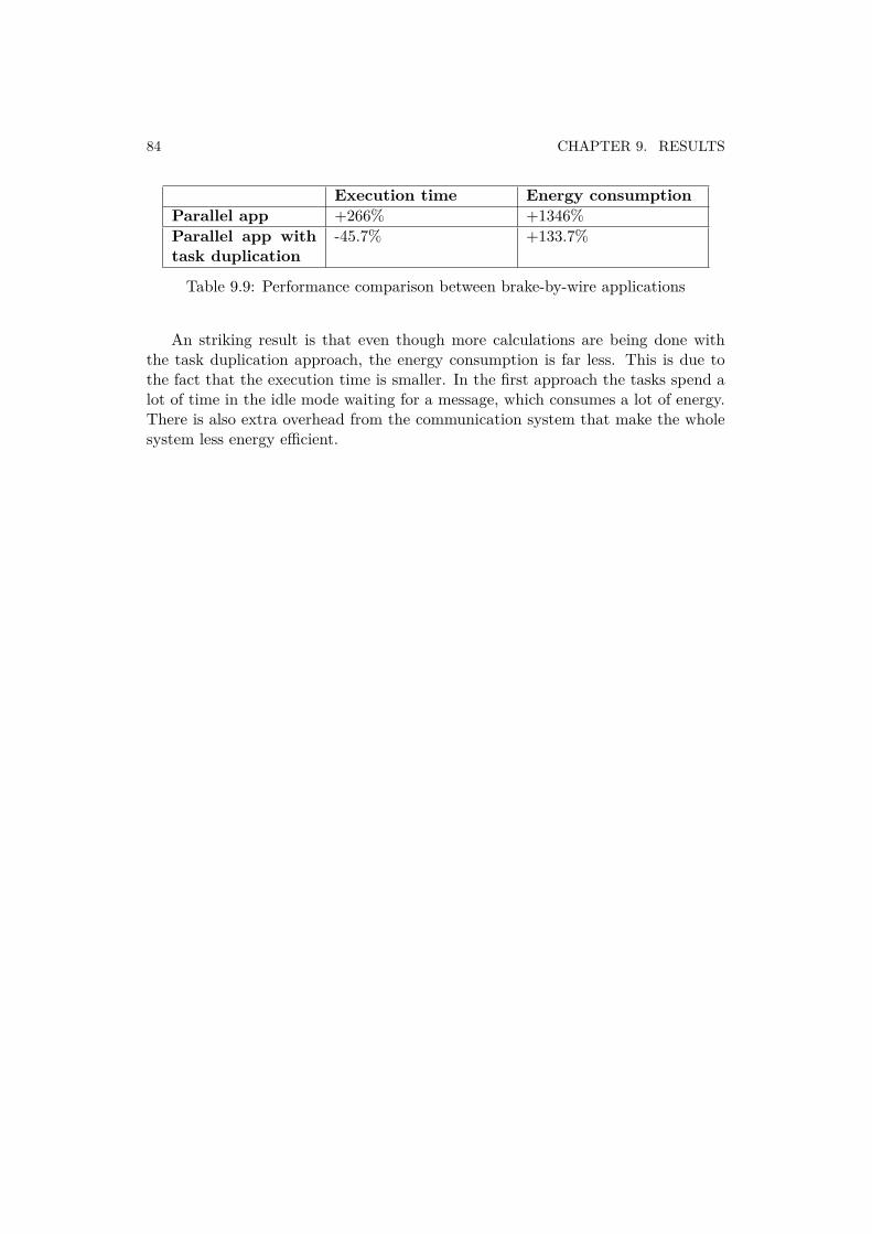
84 CHAPTER 9. RESULTS
Execution time Energy consumptionParallel app +266% +1346%Parallel app withtask duplication
-45.7% +133.7%
Table 9.9: Performance comparison between brake-by-wire applications
An striking result is that even though more calculations are being done withthe task duplication approach, the energy consumption is far less. This is due tothe fact that the execution time is smaller. In the first approach the tasks spend alot of time in the idle mode waiting for a message, which consumes a lot of energy.There is also extra overhead from the communication system that make the wholesystem less energy efficient.

Chapter 10
Conclusions and future work
10.1 ConclusionsThe goal of this project was to research scheduling algorithms for multi-core embed-ded systems and to make an implementation of a scheduler for a parallel application.In the analytical phase several algorithms have been studied and compared. Thelinear clustering algorithm was chosen to be implemented.
In the practical phase a toolchain for programming parallel applications wasimplemented. The target platform was the Epiphany E16 development board. Dif-ferent software modules for that target had to be implemented: epiphany module,file system module, interrupts module, mailbox module, host communication moduleand profiler module.
Several experiments were carried out in order to help evaluate the performanceof the system. Parallel computing should only be used when there is enough com-putation to be parallelized. If there is little parallelization to be done, the mailboxsystem is not worthy to use. However, the execution can still be sped up by usingalgorithms based on task duplication. A mailbox system is worthy to use in appli-cations with a lot of parallelization because the communication overhead can thenbe neglected.
10.2 LimitationsAt the current stage there are some limitations in the system:
• An application with more than 16 clusters cannot be handled since only onecluster is assigned to a core.
• No more than 32 blocks or 32 messages can be stored in the mailbox.
10.3 Future workSome lines of future research are:
85

86 CHAPTER 10. CONCLUSIONS AND FUTURE WORK
• Evaluation of the toolchain on other applications with different characteristics,such as execution times, communication times, CCR or DAG topology.
• Design of a more scalable system (limitation to 16 clusters, limitation to 32messages simultaneously in the mailbox).
• Implementation of other scheduling algorithms in the toolchain. Selection ofthe algorithm with the shortest makespan for each case.
• Automation of the generation of DAGs by extracting parallelism from thesource code of serial applications. This could be done by profiling the appli-cation at run-time (hotspots in the code, accesses to the memory) and usingmachine learning techniques.
• Implementation of an automatic feedback mechanism with the profiled data.It would get hold of the real execution and communication times of the ap-plication, assuming constant execution times. The original DAG would beupdated with these values increasing its fidelity. These feedback mechanismwould also validate the parameters in each execution.
• Dealing with varying execution and communication times in the system.
• Implementation of a multicast service in order not to send the same messageseveral times.
• Dynamic loading of tasks and evaluation of its performance.

Appendix A
Epiphany power consumption testapplication
In this appendix the program to measure the power consumption of the Epiphanychip as a function of the number of idle cores is attached. The program has been run17 times, changing the number of cores in idle. The cores that are not in idle stateperform operations in the Floating-Point Unit (FPU). The timers are also startedin order to consume more.
Power consumption test
1 int mc_core_common_go ( )2 3 int s t a tu s = 0 ;45 int core Id = e_get_coreid ( ) ;67 i f ( core_num( core Id )>=0)8 9 asm volat i le ( " i d l e " ) ;
10 else 11 double i , k , l , m , n ;1213 l =3.14;14 m = 3 .14567 ;15 n = 3 . 0 1 4 ;16 k = 0 ;17 i = 1 . 3 4 ;1819 while (1 )20 21 m = ( i ∗ 3 . 14 ) / 0 .57 + 32 . 5 45 ;
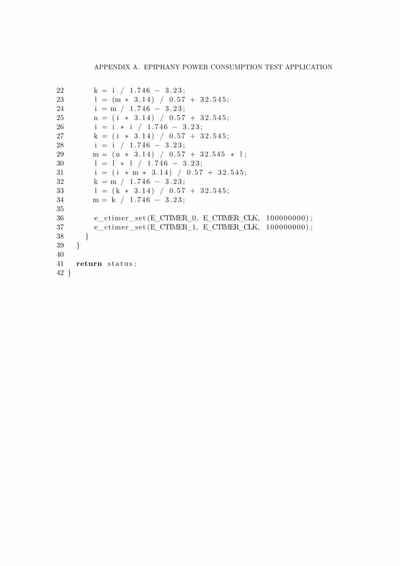
APPENDIX A. EPIPHANY POWER CONSUMPTION TEST APPLICATION
22 k = i / 1 .746 − 3 . 2 3 ;23 l = (m ∗ 3 . 14 ) / 0 .57 + 32 . 5 45 ;24 i = m / 1.746 − 3 . 2 3 ;25 n = ( i ∗ 3 . 14 ) / 0 .57 + 32 . 5 45 ;26 i = i ∗ i / 1 .746 − 3 . 2 3 ;27 k = ( i ∗ 3 . 14 ) / 0 .57 + 32 . 5 45 ;28 i = i / 1 .746 − 3 . 2 3 ;29 m = (n ∗ 3 . 14 ) / 0 .57 + 32.545 ∗ l ;30 l = l ∗ l / 1 .746 − 3 . 2 3 ;31 i = ( i ∗ m ∗ 3 . 14 ) / 0 .57 + 32 . 5 45 ;32 k = m / 1.746 − 3 . 2 3 ;33 l = (k ∗ 3 . 14 ) / 0 .57 + 32 . 5 45 ;34 m = k / 1.746 − 3 . 2 3 ;3536 e_ctimer_set (E_CTIMER_0, E_CTIMER_CLK, 100000000) ;37 e_ctimer_set (E_CTIMER_1, E_CTIMER_CLK, 100000000) ;38 39 4041 return s t a tu s ;42

Appendix B
Brake-by-wire application: single core
In this appendix a serial version of the brake-by-wire application is attached.
Single core application
1 int driver_required_brake_torque = (MAX_BRAKE_TORQUE ∗input_1 . brake_pedal_percentage ) / 100 ;
2 int dr ive r_requ i red_throt t l e_torque =(MAX_THROTTLE_TORQUE ∗input_1 . thrott l e_peda l_percentage ) / 100 ;
34 int wheel_torque = −1;5 i f (MAX_BRAKE_TORQUE/10 > driver_required_brake_torque )6 7 wheel_torque = dr iver_requ i red_throt t l e_torque / 4 ;8 else 9 wheel_torque = 0 ;
10 11 output_1 . e l_s ignal_tract ion_motor = ( wheel_torque ∗
245) /750 + 10 ;1213 int wheel_1_speed_rpm = (MAX_RPM ∗
input_1 . wheel_1_speed_rpm_percentage ) / 100 ;14 int wheel_2_speed_rpm = (MAX_RPM ∗
input_1 . wheel_2_speed_rpm_percentage ) / 100 ;15 int wheel_3_speed_rpm = (MAX_RPM ∗
input_1 . wheel_3_speed_rpm_percentage ) / 100 ;16 int wheel_4_speed_rpm = (MAX_RPM ∗
input_1 . wheel_4_speed_rpm_percentage ) / 100 ;1718 double vehicle_speed_mps = (wheel_1_speed_rpm +
wheel_2_speed_rpm + wheel_3_speed_rpm +

APPENDIX B. BRAKE-BY-WIRE APPLICATION: SINGLE CORE
wheel_4_speed_rpm)19 ∗ WHEEL_RADIOUS ∗ 2 ∗ 3 .14 / 1000 / 60 / 4 ;2021 double wheel_1_slip = ( vehicle_speed_mps −
wheel_1_speed_rpm ∗ WHEEL_RADIOUS ∗ 2 ∗ 3 .14 / 60 /1000) / vehicle_speed_mps ;
22 i f (0 > wheel_1_slip )23 wheel_1_slip = 0 ;24 double wheel_2_slip = ( vehicle_speed_mps −
wheel_2_speed_rpm ∗ WHEEL_RADIOUS ∗ 2 ∗ 3 .14 / 60 /1000) / vehicle_speed_mps ;
25 i f (0 > wheel_2_slip )26 wheel_2_slip = 0 ;27 double wheel_3_slip = ( vehicle_speed_mps −
wheel_3_speed_rpm ∗ WHEEL_RADIOUS ∗ 2 ∗ 3 .14 / 60 /1000) / vehicle_speed_mps ;
28 i f (0 > wheel_3_slip )29 wheel_3_slip = 0 ;30 double wheel_4_slip = ( vehicle_speed_mps −
wheel_4_speed_rpm ∗ WHEEL_RADIOUS ∗ 2 ∗ 3 .14 / 60 /1000) / vehicle_speed_mps ;
31 i f (0 > wheel_4_slip )32 wheel_4_slip = 0 ;3334 int abs_brake_torque_1 , abs_brake_torque_2 ,
abs_brake_torque_3 , abs_brake_torque_4 = −1;3536 i f ( (10 <= vehicle_speed_mps ∗3600/1000) && (0 . 2 <
wheel_1_slip ) )37 38 abs_brake_torque_1 = 0 ;39 else 40 abs_brake_torque_1 = driver_required_brake_torque / 4 ;41 42 output_1 . el_signal_brake_motor_1 = ( abs_brake_torque_1 ∗
245) /750 + 10 ;43 i f ( (10 <= vehicle_speed_mps ∗3600/1000) && (0 . 2 <
wheel_2_slip ) )44 45 abs_brake_torque_2 = 0 ;46 else 47 abs_brake_torque_2 = driver_required_brake_torque / 4 ;48 49 output_1 . el_signal_brake_motor_2 = ( abs_brake_torque_2 ∗

245) /750 + 10 ;50 i f ( (10 <= vehicle_speed_mps ∗3600/1000) && (0 . 2 <
wheel_3_slip ) )51 52 abs_brake_torque_3 = 0 ;53 else 54 abs_brake_torque_3 = driver_required_brake_torque / 4 ;55 56 output_1 . el_signal_brake_motor_3 = ( abs_brake_torque_3 ∗
245) /750 + 10 ;57 i f ( (10 <= vehicle_speed_mps ∗3600/1000) && (0 . 2 <
wheel_4_slip ) )58 59 abs_brake_torque_4 = 0 ;60 else 61 abs_brake_torque_4 = driver_required_brake_torque / 4 ;62 63 output_1 . el_signal_brake_motor_4 = ( abs_brake_torque_4 ∗
245) /750 + 10 ;


Appendix C
Brake-by-wire application: tasks
In this appendix the calculations’ sections of the tasks are listed. Task 6, 7 and 8are omitted due to their similarity to task 5. Task 10, 11 and 12 are omitted dueto their similarity to task 9.
Task 1
1 edge_12 . dr iver_requ i red_throt t l e_torque =(MAX_THROTTLE_TORQUE ∗input_1 . thrott l e_peda l_percentage ) / 100 ;
Task 2
1 int wheel_torque = −1;2 i f (MAX_BRAKE_TORQUE/10 >
edge_32 . dr iver_required_brake_torque )3 4 wheel_torque = edge_12 . dr ive r_requ i red_throt t l e_torque /
4 ;5 else 6 wheel_torque = 0 ;7 8 output_2 . e l_s ignal_tract ion_motor = ( wheel_torque ∗
245) /750 + 10 ;
Task 3
1 int driver_required_brake_torque = (MAX_BRAKE_TORQUE ∗input_3 . brake_pedal_percentage ) / 100 ;
2 edge_32 . dr iver_required_brake_torque =driver_required_brake_torque ;
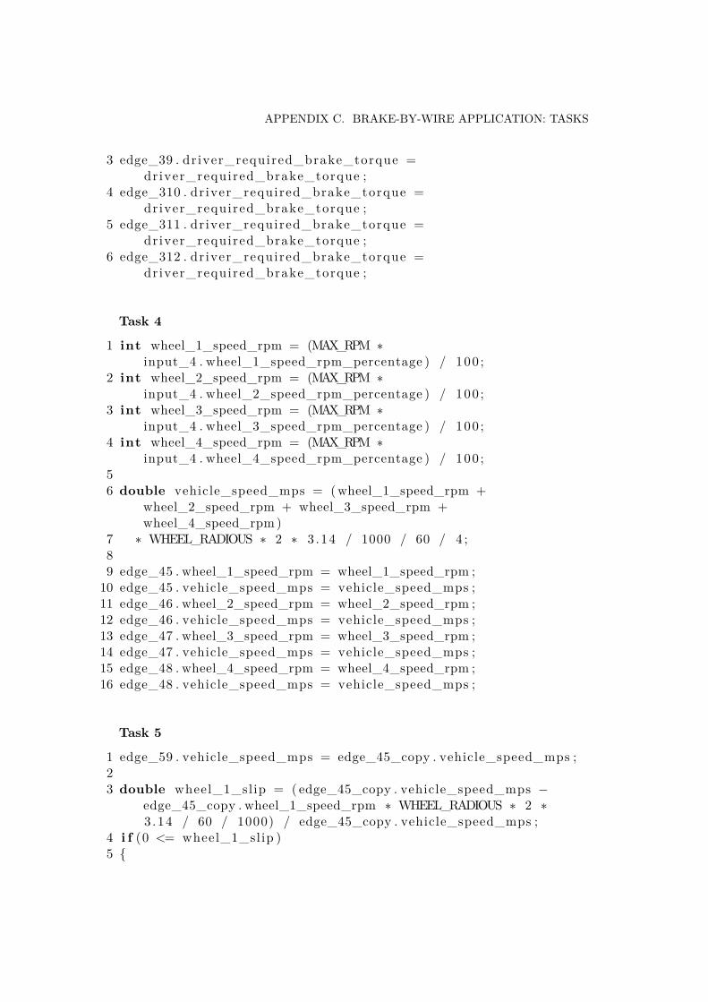
APPENDIX C. BRAKE-BY-WIRE APPLICATION: TASKS
3 edge_39 . dr iver_required_brake_torque =driver_required_brake_torque ;
4 edge_310 . dr iver_required_brake_torque =driver_required_brake_torque ;
5 edge_311 . dr iver_required_brake_torque =driver_required_brake_torque ;
6 edge_312 . dr iver_required_brake_torque =driver_required_brake_torque ;
Task 4
1 int wheel_1_speed_rpm = (MAX_RPM ∗input_4 . wheel_1_speed_rpm_percentage ) / 100 ;
2 int wheel_2_speed_rpm = (MAX_RPM ∗input_4 . wheel_2_speed_rpm_percentage ) / 100 ;
3 int wheel_3_speed_rpm = (MAX_RPM ∗input_4 . wheel_3_speed_rpm_percentage ) / 100 ;
4 int wheel_4_speed_rpm = (MAX_RPM ∗input_4 . wheel_4_speed_rpm_percentage ) / 100 ;
56 double vehicle_speed_mps = (wheel_1_speed_rpm +
wheel_2_speed_rpm + wheel_3_speed_rpm +wheel_4_speed_rpm)
7 ∗ WHEEL_RADIOUS ∗ 2 ∗ 3 .14 / 1000 / 60 / 4 ;89 edge_45 . wheel_1_speed_rpm = wheel_1_speed_rpm ;
10 edge_45 . vehicle_speed_mps = vehicle_speed_mps ;11 edge_46 . wheel_2_speed_rpm = wheel_2_speed_rpm ;12 edge_46 . vehicle_speed_mps = vehicle_speed_mps ;13 edge_47 . wheel_3_speed_rpm = wheel_3_speed_rpm ;14 edge_47 . vehicle_speed_mps = vehicle_speed_mps ;15 edge_48 . wheel_4_speed_rpm = wheel_4_speed_rpm ;16 edge_48 . vehicle_speed_mps = vehicle_speed_mps ;
Task 5
1 edge_59 . vehicle_speed_mps = edge_45_copy . vehicle_speed_mps ;23 double wheel_1_slip = ( edge_45_copy . vehicle_speed_mps −
edge_45_copy . wheel_1_speed_rpm ∗ WHEEL_RADIOUS ∗ 2 ∗3 .14 / 60 / 1000) / edge_45_copy . vehicle_speed_mps ;
4 i f (0 <= wheel_1_slip )5

6 edge_59 . wheel_1_slip = wheel_1_slip ;7 else 8 edge_59 . wheel_1_slip = 0 ;9
Task 9
1 int abs_brake_torque = −1;2 i f ( (10 <= edge_59_copy . vehicle_speed_mps ∗3600/1000) && (0 . 2
< edge_59_copy . wheel_1_slip ) )3 4 abs_brake_torque = 0 ;5 else 6 abs_brake_torque = edge_39 . dr iver_required_brake_torque /
4 ;7 8 output_9 . el_signal_brake_motor_1 = ( abs_brake_torque ∗
245) /750 + 10 ;


Appendix D
Brake-by-wire application with taskduplication: tasks
In this appendix the calculations’ sections of the tasks are listed. Task 5, 6 and 7are omitted due to their similarity to task 4.
Task 11 int driver_required_brake_torque = (MAX_BRAKE_TORQUE ∗
input_1 . brake_pedal_percentage ) / 100 ;2 edge_1 . dr iver_required_brake_torque =
driver_required_brake_torque ;
Task 21 int wheel_torque = −1;2 int dr ive r_requ i red_throt t l e_torque = (MAX_THROTTLE_TORQUE
∗ input_2 . thrott l e_peda l_percentage ) / 100 ;3 i f (MAX_BRAKE_TORQUE/10 >
edge_1 . dr iver_required_brake_torque )4 5 wheel_torque = dr iver_requ i red_throt t l e_torque / 4 ;6 else 7 wheel_torque = 0 ;8 9 output_2 . e l_s ignal_tract ion_motor = ( wheel_torque ∗
245) /750 + 10 ;
Task 31 int wheel_1_speed_rpm = (MAX_RPM ∗
input_3456 . wheel_1_speed_rpm_percentage ) / 100 ;

APPENDIX D. BRAKE-BY-WIRE APPLICATION WITH TASK DUPLICATION:TASKS
2 int wheel_2_speed_rpm = (MAX_RPM ∗input_3456 . wheel_2_speed_rpm_percentage ) / 100 ;
3 int wheel_3_speed_rpm = (MAX_RPM ∗input_3456 . wheel_3_speed_rpm_percentage ) / 100 ;
4 int wheel_4_speed_rpm = (MAX_RPM ∗input_3456 . wheel_4_speed_rpm_percentage ) / 100 ;
56 double vehicle_speed_mps = (wheel_1_speed_rpm +
wheel_2_speed_rpm + wheel_3_speed_rpm +wheel_4_speed_rpm)
7 ∗ WHEEL_RADIOUS ∗ 2 ∗ 3 .14 / 1000 / 60 / 4 ;89 edge_34 . wheel_1_speed_rpm = wheel_1_speed_rpm ;
10 edge_34 . vehicle_speed_mps = vehicle_speed_mps ;
Task 4
1 double wheel_1_slip = ( edge_34 . vehicle_speed_mps −edge_34 . wheel_1_speed_rpm ∗ WHEEL_RADIOUS ∗ 2 ∗ 3 .14 /60 / 1000) / edge_34 . vehicle_speed_mps ;
2 i f (0 > wheel_1_slip )3 4 wheel_1_slip = 0 ;5 67 int abs_brake_torque = −1;8 i f ( (10 <= edge_34 . vehicle_speed_mps ∗3600/1000) && (0 . 2 <
wheel_1_slip ) )9
10 abs_brake_torque = 0 ;11 else 12 abs_brake_torque = edge_1 . dr iver_required_brake_torque /
4 ;13 14 output_4 . el_signal_brake_motor_1 = ( abs_brake_torque ∗
245) /750 + 10 ;

Bibliography
[1] T. Hagras and J. Janeek, “Static vs. dinamic list-scheduling performance com-parison,” Acta Polytechnica, vol. 43, no. 6, 2003.
[2] J. Markoff, “Intel’s big shift after hitting technical wall,” New York Times,2004.
[3] M. J. Bridges, N. Vachharajani, Y. Zhang, T. Jablin, and D. I. August, “Revis-iting the sequential programming model for multi-core,” in Microarchitecture,2007. MICRO 2007. 40th Annual IEEE/ACM International Symposium on,pp. 69–84, IEEE, 2007.
[4] C. E. Frank J. Bartos, P.E., “Growing applications for multi-core processors.”http://www.controleng.com/index.php?id=483&cHash=081010&tx_ttnews%5Btt_news%5D=42947.
[5] D. Geer, “Chip makers turn to multicore processors,” Computer, vol. 38, no. 5,pp. 11–13, 2005.
[6] C. E. Frank J. Bartos, P.E., “Computing power:Multi-core processors help industrial automation.”http://www.controleng.com/index.php?id=483&cHash=081010&tx_ttnews[tt_news]=43096.
[7] I. C. Ian Gilvarry, “Insights on multi-core processors.”http://www.controleng.com/single-article/insights-on-multi-core-processors/db06fb5f14b0f011155f96c80259038b.html.
[8] Y. Choi, Y. Lin, N. Chong, S. Mahlke, and T. Mudge, “Stream compilation forreal-time embedded multicore systems,” in Code Generation and Optimization,2009. CGO 2009. International Symposium on, pp. 210–220, IEEE, 2009.
[9] C. LUCAR, Dataflow Programming for Systems Design Space Exploration forMulticore Platforms. PhD thesis, ÉCOLE POLYTECHNIQUE FÉDÉRALEDE LAUSANNE, 2011.
[10] M. J. Flynn, “Very high-speed computing systems,” Proceedings of the IEEE,vol. 54, no. 12, pp. 1901–1909, 1966.

BIBLIOGRAPHY
[11] C. W. page, “Autosar.” http://www.autosar.org.
[12] A. Sangiovanni-Vincentelli and M. Di Natale, “Embedded system design forautomotive applications,” Computer, vol. 40, no. 10, pp. 42–51, 2007.
[13] S. Chakraborty, M. Di Natale, H. Falk, M. Lukasiewycz, and F. Slomka, “Tim-ing and schedulability analysis for distributed automotive control applications,”in Proceedings of the ninth ACM international conference on Embedded soft-ware, pp. 349–350, ACM, 2011.
[14] S. K. Jena and M. Srinivas, “On the suitability of multi-core processing forembedded automotive systems,” in Cyber-Enabled Distributed Computing andKnowledge Discovery (CyberC), 2012 International Conference on, pp. 315–322, IEEE, 2012.
[15] A. Monot, N. Navet, B. Bavoux, F. Simonot-Lion, et al., “Multicore schedulingin automotive ecus,” in Embedded Real Time Software and Systems-ERTSS2010, 2010.
[16] N. Navet, A. Monot, B. Bavoux, F. Simonot-Lion, et al., “Multi-source andmulticore automotive ecus-os protection mechanisms and scheduling,” in In-ternational Symposium on Industrial Electronics-ISIE 2010, 2010.
[17] A. Monot, N. Navet, B. Bavoux, and F. Simonot-Lion, “Multisource software onmulticore automotive ecus—combining runnable sequencing with task schedul-ing,” Industrial Electronics, IEEE Transactions on, vol. 59, no. 10, pp. 3934–3942, 2012.
[18] H. Kopetz, R. Obermaisser, C. El Salloum, and B. Huber, “Automotive soft-ware development for a multi-core system-on-a-chip,” in Software Engineeringfor Automotive Systems, 2007. ICSE Workshops SEAS’07. Fourth Interna-tional Workshop on, pp. 2–2, IEEE, 2007.
[19] S. Schliecker, J. Rox, M. Negrean, K. Richter, M. Jersak, and R. Ernst, “Systemlevel performance analysis for real-time automotive multicore and network ar-chitectures,” Computer-Aided Design of Integrated Circuits and Systems, IEEETransactions on, vol. 28, no. 7, pp. 979–992, 2009.
[20] N. Böhm, D. Lohmann, W. Schröder-Preikschat, and F. Erlangen-Nürnberg,“Multi-core processors in the automotive domain: An autosar case study,”Proceedings Work-in-Progress Session, 2010.
[21] J. Schneider, M. Bohn, and R. Rößger, “Migration of automotive real-time soft-ware to multicore systems: First steps towards an automated solution,” in theProceedings of the Work-in-Progress Session of the 22nd Euromicro Conferenceon Real-Time Systems (ECRTS), 2010.

BIBLIOGRAPHY
[22] T. Wei, Z. Qiu, C. Young, and D. Chang, “Development of heterogeneous mul-ticore embedded platform for automotive applications,” in 2011 InternationalConference on Circuits, System and Simulation (IPCSIT), vol. 7, 2011.
[23] 2carpros Web page, “How abs anti-lock brake systems work.”http://www.2carpros.com/articles/how-abs-anti-lock-brakes-work.
[24] W. Xiang, P. C. Richardson, C. Zhao, and S. Mohammad, “Automobile brake-by-wire control system design and analysis,” Vehicular Technology, IEEETransactions on, vol. 57, no. 1, pp. 138–145, 2008.
[25] T. Nolte, H. Hansson, and L. L. Bello, “Automotive communications-past,current and future,” in Emerging Technologies and Factory Automation, 2005.ETFA 2005. 10th IEEE Conference on, vol. 1, pp. 8–pp, IEEE, 2005.
[26] A. Davare, Q. Zhu, M. Di Natale, C. Pinello, S. Kanajan, and A. Sangiovanni-Vincentelli, “Period optimization for hard real-time distributed automotivesystems,” in Proceedings of the 44th annual Design Automation Conference,pp. 278–283, ACM, 2007.
[27] A. Rajeev, S. Mohalik, M. G. Dixit, D. B. Chokshi, and S. Ramesh, “Schedula-bility and end-to-end latency in distributed ecu networks: formal modeling andprecise estimation,” in Proceedings of the tenth ACM international conferenceon Embedded software, pp. 129–138, ACM, 2010.
[28] D. Goswami, R. Schneider, and S. Chakraborty, “Co-design of cyber-physicalsystems via controllers with flexible delay constraints,” in Proceedings of the16th Asia and South Pacific Design Automation Conference, pp. 225–230, IEEEPress, 2011.
[29] P. Sinha, “Architectural design and reliability analysis of a fail-operationalbrake-by-wire system from iso 26262 perspectives,” Reliability Engineering &System Safety, vol. 96, no. 10, pp. 1349–1359, 2011.
[30] A. Suleman, “Q & a: Do multicores save energy? not re-ally.” http://www.futurechips.org/chipdesignforall/amulticoresaveenergy.html,2011.
[31] B. Kreeley and S. Coulton, “Increasing the lifes-pan and reliability of electrical components.”http://www.ospmag.com/files/pdf/whitepaper/Kooltronics_WP.pdf.
[32] A. Grama, Introduction to parallel computing. Addison Wesley, 2003.
[33] P. Pacheco, An introduction to parallel programming. Morgan Kaufmann, 2011.
[34] G. R. Andrews, “Foundations of multithreaded, parallel, and distributed pro-gramming. 2000,” Wesley, University of Arizona, USA.

BIBLIOGRAPHY
[35] T. G. Mattson, B. A. Sanders, and B. L. Massingill, Patterns for parallel pro-gramming. Addison-Wesley Professional, 2004.
[36] W. Barry, Parallel Programming: Techniques and Applications Using Net-worked Workstations and Parallel Computers, 2/E. Pearson Education India,2006.
[37] O. Sinnen, L. A. Sousa, and F. E. Sandnes, “Toward a realistic task schedulingmodel,” Parallel and Distributed Systems, IEEE Transactions on, vol. 17, no. 3,pp. 263–275, 2006.
[38] A. Olteanu and A. Marin, “Generation and evaluation of scheduling dags: Howto provide similar evaluation conditions,” Computer Science Master Research,vol. 1, no. 1, pp. 57–66, 2011.
[39] U. Banerjee, R. Eigenmann, A. Nicolau, and D. A. Padua, “Automatic programparallelization,” Proceedings of the IEEE, vol. 81, no. 2, pp. 211–243, 1993.
[40] Wikipedia, “Openmp.” http://en.wikipedia.org/wiki/OpenMP.
[41] Wikipedia, “Openhmpp.” http://en.wikipedia.org/wiki/OpenHMPP.
[42] C. T. M.-C. P. Company, “Caps compilers.” http://www.caps-entreprise.com/products/caps-compilers/.
[43] C. C. F. Bodin, “Programming heterogeneous many-cores using directives.”http://cs.ioc.ee/etaps12/invited/bodin-slides.pdf.
[44] J. D. Ullman, “< i> np</i>-complete scheduling problems,” Journal of Com-puter and System sciences, vol. 10, no. 3, pp. 384–393, 1975.
[45] M. T. C. S. JIS, “Computers and intractability a guide to the theory of np-completeness,” 1979.
[46] O. Sinnen, Task scheduling for parallel systems, vol. 60. Wiley-Interscience,2007.
[47] P. Chrétienne, “Task scheduling with interprocessor communication delays,”European Journal of Operational Research, vol. 57, no. 3, pp. 348–354, 1992.
[48] I. Ahmad, Y.-K. Kwok, and M.-Y. Wu, “Analysis, evaluation, and comparisonof algorithms for scheduling task graphs on parallel processors,” in Parallel Ar-chitectures, Algorithms, and Networks, 1996. Proceedings. Second InternationalSymposium on, pp. 207–213, IEEE, 1996.
[49] Y.-K. Kwok and I. Ahmad, “Benchmarking and comparison of the task graphscheduling algorithms,” Journal of Parallel and Distributed Computing, vol. 59,no. 3, pp. 381–422, 1999.
BIBLIOGRAPHY
[50] Y.-K. Kwok and I. Ahmad, “Static scheduling algorithms for allocating directedtask graphs to multiprocessors,” ACM Computing Surveys (CSUR), vol. 31,no. 4, pp. 406–471, 1999.
[51] N. Arora, “Analysis and performance comparison of algorithms for schedulingdirected task graphs to parallel processors,” ANALYSIS, vol. 4, no. 2, 2012.
[52] T. L. Adam, K. M. Chandy, and J. Dickson, “A comparison of list schedulesfor parallel processing systems,” Communications of the ACM, vol. 17, no. 12,pp. 685–690, 1974.
[53] M.-Y. Wu and D. D. Gajski, “Hypertool: A programming aid for message-passing systems,” Parallel and Distributed Systems, IEEE Transactions on,vol. 1, no. 3, pp. 330–343, 1990.
[54] J.-J. Hwang, Y.-C. Chow, F. D. Anger, and C.-Y. Lee, “Scheduling precedencegraphs in systems with interprocessor communication times,” SIAM Journalon Computing, vol. 18, no. 2, pp. 244–257, 1989.
[55] G. C. Sih and E. A. Lee, “A compile-time scheduling heuristic forinterconnection-constrained heterogeneous processor architectures,” Paralleland Distributed Systems, IEEE Transactions on, vol. 4, no. 2, pp. 175–187,1993.
[56] A. Olteanu, F. Pop, C. Dobre, and V. Cristea, “A dynamic rescheduling algo-rithm for resource management in large scale dependable distributed systems,”Computers & Mathematics with Applications, vol. 63, no. 9, pp. 1409 – 1423,2012.
[57] V. Sarkar, Partitioning and scheduling parallel programs for multiprocessors.MIT press, 1989.
[58] S. Kim and J. Browne, “A general approach to mapping of parallel computationupon multiprocessor architectures,” in International Conference on ParallelProcessing, vol. 3, p. 8, 1988.
[59] T. Yang and A. Gerasoulis, “Dsc: Scheduling parallel tasks on an unboundednumber of processors,” Parallel and Distributed Systems, IEEE Transactionson, vol. 5, no. 9, pp. 951–967, 1994.
[60] Y.-K. Kwok and I. Ahmad, “A static scheduling algorithm using dynamic crit-ical path for assigning parallel algorithms onto multiprocessors,” in ParallelProcessing, 1994. ICPP 1994. International Conference on, vol. 2, pp. 155–159, IEEE, 1994.
[61] H. El-Rewini and T. G. Lewis, “Scheduling parallel program tasks onto arbi-trary target machines,” Journal of parallel and Distributed Computing, vol. 9,no. 2, pp. 138–153, 1990.
BIBLIOGRAPHY
[62] N. Mehdiratta and K. Ghose, “A bottom-up approach to task scheduling ondistributed memory multiprocessors,” in Parallel Processing, 1994. ICPP 1994.International Conference on, vol. 2, pp. 151–154, IEEE, 1994.
[63] K. Ghose and N. Mehdiratta, “A universal approach for task scheduling fordistributed memory multiprocessors,” in Scalable High-Performance Comput-ing Conference, 1994., Proceedings of the, pp. 577–584, IEEE, 1994.
[64] N. Mehdiratta and K. Ghose, “Scheduling task graphs onto distributed memorymultiprocessors under realistic constraints,” PARLE’94 Parallel Architecturesand Languages Europe, pp. 589–600, 1994.
[65] O. Sinnen, A. To, and M. Kaur, “Contention-aware scheduling with task dupli-cation,” Journal of Parallel and Distributed Computing, vol. 71, no. 1, pp. 77–86, 2011.
[66] Y.-K. Kwok and I. Ahmad, “Bubble scheduling: A quasi dynamic algorithm forstatic allocation of tasks to parallel architectures,” in Parallel and DistributedProcessing, 1995. Proceedings. Seventh IEEE Symposium on, pp. 36–43, IEEE,1995.
[67] A. B. Kahn, “Topological sorting of large networks,” Communications of theACM, vol. 5, no. 11, pp. 558–562, 1962.
[68] A. Inc., “Epiphany architecture reference (g3).” http://www.adapteva.com/wp-content/uploads/2012/12/epiphany_arch_reference_3.12.12.18.pdf.