Analysis Tool for Fast Power System Steady-State Angular ...
31
Analysis Tool for Fast Power System Steady-State Angular Stability Assessment Final Project Report S-85G Power Systems Engineering Research Center Empowering Minds to Engineer the Future Electric Energy System
Transcript of Analysis Tool for Fast Power System Steady-State Angular ...

Analysis Tool for Fast Power System Steady-State
Angular Stability Assessment
Final Project Report
S-85G
Power Systems Engineering Research Center
Empowering Minds to Engineer the Future Electric Energy System
Analysis Tool for Fast Power System Steady-State
Angular Stability Assessment
Final Project Report
Project Team
Le Xie, Project Leader
Texas A&M University
Postdoctoral Researcher
Bin Wang
Texas A&M University
PSERC Publication 20-02
April 2020

For information about this project, contact:
Le Xie
Department of Electrical and Computer Engineering
Texas A&M University
College Station, TX 77843
Phone: 979-845-7563
Fax: 979-845-6259
Email: [email protected]
Power Systems Engineering Research Center
The Power Systems Engineering Research Center (PSERC) is a multi-university Center
conducting research on challenges facing the electric power industry and educating the next
generation of power engineers. More information about PSERC can be found at the Center’s
website: http://www.pserc.org.
For additional information, contact:
Power Systems Engineering Research Center
Arizona State University
527 Engineering Research Center
Tempe, Arizona 85287-5706
Phone: 480-965-1643
Fax: 480-727-2052
Notice Concerning Copyright Material
PSERC members are given permission to copy without fee all or part of this publication for internal
use if appropriate attribution is given to this document as the source material. This report is
available for downloading from the PSERC website.
© 2020 Texas A&M University. All rights reserved.

i
Acknowledgements
The investigators acknowledge the financial and technical support from engineers at ISO New
England, Dr. Slava Maslennikov, Dr. Xiaochuan Luo, Mr. Qiang Zhang and Dr. Mingguo Hong.
Special thanks are extended to other engineers at ISO New England, including Dr. Tongxin Zheng,
and Dr. Eugene Litvinov, for the insightful and fruitful discussions.

ii
Executive Summary
Determining reliable actionable limits for phase angles measured by Phasor Measurement Units
can help trigger remedial control actions in a timely fashion to avoid system blackouts. Traditional
ways for calculating the steady- state stability limits always require manually selected interfaces
and a pre-defined methodology for system stressing. However, there is no systematic way or
NERC Standards for neither one. This project proposes and validates a novel analytical tool for
fast assessment of power system steady-state angular stability limit, which provides a new
perspective to understand and determine the steady-state angular stability leveraging the nonlinear
information within the underlying power system dynamic model. This new tool can determine the
angle limits for all lines, i.e. naturally covering all interfaces, without calculating the nonlinear
power flow equations. This study would provide guideline for phase angle based system stability
monitoring and control. Next steps to move the research toward applications include developing
dedicated algorithms without symbolic derivations to further reduce the computation, conducting
N-1 contingency analysis and design of remedial control actions.
Project Publications:
[1] Bin Wang, Le Xie, Slava Maslennikov, Xiaochuan Luo, Qiang Zhang, Mingguo Hong, “A
model-space method for online power system steady-state stability monitoring,” IEEE
Trans. Power Systems, in preparation.

iii
Table of Contents
1. Introduction ................................................................................................................................1
1.1 Background ........................................................................................................................1
1.2 A brief review of selected stability problems ....................................................................2
1.3 Scope of work ....................................................................................................................4
1.4 Report Organization ..........................................................................................................4
2. Power System Nonlinear Dynamic Model in Modal Space ......................................................6
3. A Modal-Space Method to Estimate SSASL .............................................................................8
3.1 Simplifying nonlinear dynamic model in modal space .....................................................8
3.2 Constructing real-valued DEs for each nonlinear mode ....................................................8
3.3 Identifying generalized “power-angle curve” for each nonlinear mode ...........................9
3.4 Estimating SSASL for each nonlinear mode ...................................................................10
3.5 Determining system steady state at each limit point .......................................................10
3.6 Remarks on MS method ..................................................................................................12
3.7 Applying MS method to online stability monitoring ......................................................13
4. Case Studies .............................................................................................................................14
4.1 Tests on IEEE 9-bus power system .................................................................................14
4.2 Tests on New England 39-bus power system ..................................................................18
5. Conclusions ..............................................................................................................................21
References ......................................................................................................................................22

iv
List of Figures
Figure 1.1 Divergence of phase angle between Cleveland and Michigan during 2003 Northeast
blackout [2] ..................................................................................................................................... 1
Figure 1.2 Boundaries of voltage stability, small-signal stability and aperiodic stability in
parameter space ............................................................................................................................... 3
Figure 1.3 Aperiodic instability and self-oscillation instability ...................................................... 4
Figure 2.1 Aperiodic instability and self-oscillation instability .................................................... 10
Figure 3.1 Numerically identified stability boundaries and SSASL points estimated by MS1,
MS2 and MS3 in the 9-bus system. (VS, AS and SSS respectively represent voltage, aperiodic
and small-signal stabilities. Red stars, triangles and circles respectively represent the estimated
SSASL points by MS1, MS2 and MS 3. The green circle is the given operating condition.) ...... 15
Figure 3.2 Estimated SSASL points over stressing. ..................................................................... 17
Figure 3.3 MW margins v.s. change of 𝑃e3. ................................................................................ 18
Figure 3.4 MW margins in Scenario 1 .......................................................................................... 19
Figure 3.5 MW margins in Scenario 2 .......................................................................................... 20

v
List of Tables
Table 1.1 Comparison of MS1, MS2 and MS3 ........................................................................... 13

1
1. Introduction
1.1 Background
The principal cause of the Northeast Blackout in 2003 was a lack of situational awareness due to
inadequate reliability tools [1]. The interconnection-wide phase angles are monitored in real-time
by massive Phasor Measurement Units (PMUs) that have been deployed in the last two decades.
However, these phase angles currently are only interpreted as an indicator of the stress level
associated with the amount of power transfer through transmission lines or among control areas,
while no operating guidelines or procedures have been developed to establish reliable actionable
limits [2]. A lack of reliable actionable limits makes it difficult for the system operator to determine
when to take remedial control actions, such that generators may lose synchronism and blackouts
may happen if the system is increasingly stressed over time, such as a monitored phase angle in
2003 Northeast blackout in Figure 1.1 [3]. In North American power grids, no NERC Standards
have been established that specifically require electric utilities or operators to monitor phase angles
[4]. The reason for such missing standards largely stems from the fact that the actionable angle
limits are not constant and are difficult to determine, which highly depend on the system topology,
loading condition, generation schedule and, most importantly, the way to stress the system to
approach its steady state stability limit.
Figure 1.1 Divergence of phase angle between Cleveland and Michigan during 2003 Northeast
blackout [3]

2
The comprehensive and accurate assessment of reliability, i.e. dynamic security assessment
(DSA), requires solving computational-extensive numerical integrations which make DSA viable
only for offline planning or long-cycle online applications [5]. In practical power system planning
and operations, there are usually several thousand contingencies and tens or hundreds of interface
limits to be calculated. In addition, considering more diverse power flow patterns brought by a
high penetration of intermittent energy resources, future DSA is expected to be executed more
frequently with a shorter cycle or even approaching real-time. These trends motivate the research
needs for fast stability assessment tools to increase the situational awareness and lower the risk of
large-scale blackouts.
A promising way to address such a challenge is the steady-state stability analysis, which only
focuses on the steady-state condition of power systems such that the stability assessment can be
significantly simplified. The static stability of the base case (without any contingencies) is a
necessary condition of system stability and it has been proved practically useful [5][6], including
estimating the stability margin as well as other purposes such as the forward reserve procurement.
The basic idea is to identify the steady-state voltage stability limit (SSVSL) in a very speedy
fashion by solving static power flow equations such that SSVSL can be calculated and monitored
online. The online implementation of this type of approaches will guarantee the system operator's
awareness of the situation where a margin becomes dangerously low, allowing preparation and
execution of necessary control actions. Such an application seems to be more needed in future
grids with a high penetration of intermittent renewable energy where system conditions may
change more frequently and significantly.
However, there are three major challenges with existing methods for assessing SSVSL when
dealing with future power grid with massive renewables: (i) selection of interfaces and scenarios,
i.e. which interface is of concern and how to select the sink and the source [7][8]; (ii) need for
solving a series of power flows for each interface and for each scenario; and (iii) SSVSL is an
optimistic stability analysis since small-signal instabilities may still occur without violating
SSVSL (to be shown in case study section of this paper). Even regardless of the computational
burden involved in (ii), the selections in (i) are always conducted manually, where people’s
experiences and understanding about historic behaviors of the power grid play an important role.
Such manual selections can be either difficult or unreliable, especially when considering the power
flow pattern and critical interfaces may change more significantly and more frequently with
loading and operating conditions for future power grids with a high penetration of intermittent
distributed energy resources. To this end, an automated, fast and less-optimistic method is
proposed in this paper to estimate the steady-state angle stability limit (SSASL), which captures
the Saddle-node bifurcation points along certain stressing directions defined by the associated
linearized dynamic system. Although these stressing directions may be unrealistic, it is found by
extensive numerical studies that the stability margin defined by the proposed approach along any
realistic stressing direction would always become low when approaching the stability boundary.
1.2 A brief review of selected stability problems
This section briefly reviews a few selected power system stability problems, i.e. TSA, SSA and
static voltage stability analysis (VSA), to point out the scope of this work. The review is neither

3
exhaustive nor comprehensive, and we refer interested readers to reference [9] for a comprehensive
review of power system stability problems.
TSA of nonlinear dynamical power systems is usually considered to be the most realistic dynamic
performance analysis, which is used for benchmarking other simplified stability analyses, e.g.
small-signal and voltage stability analyses, and evaluating new control schemes, e.g. damping
controls. TSA is often defined upon a set of nonlinear differential-algebraic equations (DAEs),
whose accurate assessment by a numerical integration can be very computationally-expensive
[10]. Thus, in practical applications, numerical integration based TSA is used for most utilities,
while for some utilities it is used as the final check of very few scenarios screened out by fast but
not very accurate analyses, e.g. a direct method [11]. With today's analytical and computing
capability, it is still extremely difficult, if not impossible, to implement online TSA for analyzing
all contingencies and all potential changes in loading and generation conditions.
SSA is a common simplification of the stability analysis of nonlinear dynamical systems, which is
only valid in a small neighborhood of the equilibrium point, i.e. the steady-state condition, since
all nonlinearities with power system DAEs are ignored. To evaluate the small-signal stability of
power systems under other steady-state conditions or when subject to possible changes of loading
and generations, SSA needs to be re-executed, which is also considered to be computational-
expensive for the computing resources in today's control room.
Static voltage stability analysis (VSA) is a further simplification which ignores all dynamics, while
only retaining Kirchhoff's current and voltage laws in the power network, resulting in a set of
nonlinear algebraic equations known as power flow equations. Static VSA may imply SSA under
some extreme and unrealistic assumptions, while in general there is no such an implication
[12][13] and voltage stability is usually an optimistic estimate of small-signal stability as shown
in Figure 1.2. Most production-level solutions of power flow equations are iterative in nature, e.g.
Newton-Raphson and fast decouple methods, although computationally demanding, which are
computationally much cheaper than SSA and TSA.
Figure 1.2 Boundaries of voltage stability, small-signal stability and aperiodic stability in
parameter space
17
Voltage stability boundary
Small-signal stability
boundary
Aperiodic stability boundary
4
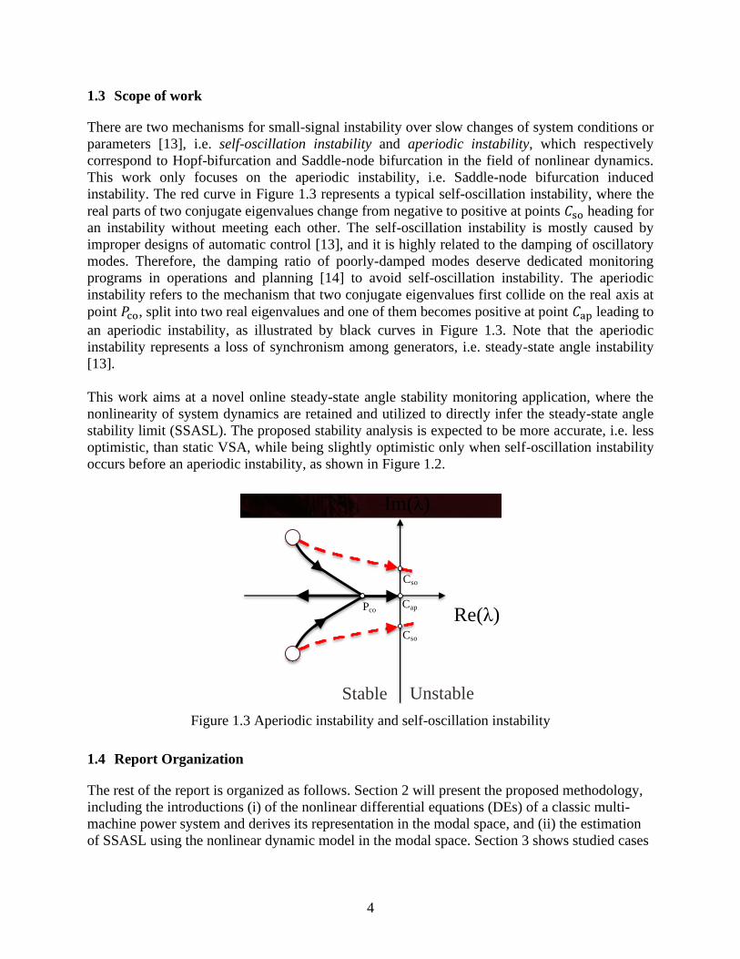
1.3 Scope of work
There are two mechanisms for small-signal instability over slow changes of system conditions or
parameters [13], i.e. self-oscillation instability and aperiodic instability, which respectively
correspond to Hopf-bifurcation and Saddle-node bifurcation in the field of nonlinear dynamics.
This work only focuses on the aperiodic instability, i.e. Saddle-node bifurcation induced
instability. The red curve in Figure 1.3 represents a typical self-oscillation instability, where the
real parts of two conjugate eigenvalues change from negative to positive at points 𝐶so heading for
an instability without meeting each other. The self-oscillation instability is mostly caused by
improper designs of automatic control [13], and it is highly related to the damping of oscillatory
modes. Therefore, the damping ratio of poorly-damped modes deserve dedicated monitoring
programs in operations and planning [14] to avoid self-oscillation instability. The aperiodic
instability refers to the mechanism that two conjugate eigenvalues first collide on the real axis at
point 𝑃co, split into two real eigenvalues and one of them becomes positive at point 𝐶ap leading to
an aperiodic instability, as illustrated by black curves in Figure 1.3. Note that the aperiodic
instability represents a loss of synchronism among generators, i.e. steady-state angle instability
[13].
This work aims at a novel online steady-state angle stability monitoring application, where the
nonlinearity of system dynamics are retained and utilized to directly infer the steady-state angle
stability limit (SSASL). The proposed stability analysis is expected to be more accurate, i.e. less
optimistic, than static VSA, while being slightly optimistic only when self-oscillation instability
occurs before an aperiodic instability, as shown in Figure 1.2.
Figure 1.3 Aperiodic instability and self-oscillation instability
1.4 Report Organization
The rest of the report is organized as follows. Section 2 will present the proposed methodology,
including the introductions (i) of the nonlinear differential equations (DEs) of a classic multi-
machine power system and derives its representation in the modal space, and (ii) the estimation
of SSASL using the nonlinear dynamic model in the modal space. Section 3 shows studied cases
16
Re(λ)
Im(λ)
Stable Unstable
Cso
Cap
Cso
Pco

5
on the IEEE 9-bus and 39-bus power systems to validate the proposed approach. Section 4 draws
conclusions and envisions future works.

6
2. Power System Nonlinear Dynamic Model in Modal Space
Consider a classic 𝑁-machine power system
{�̇�𝑖 = 𝜔s𝜔𝑖
�̇�𝑖 =1
2𝐻𝑖(𝑃m𝑖 − 𝑃e𝑖 −𝐷𝑖𝜔𝑖)
(1)
𝑃e𝑖 = 𝐸𝑖2𝐺𝑖 − ∑
𝑁𝑗=1,𝑗≠𝑖 (𝐶𝑖𝑗sin(𝛿𝑖 − 𝛿𝑗 − 𝛿s𝑖𝑗) + 𝐷𝑖𝑗cos(𝛿𝑖 − 𝛿𝑗 − 𝛿s𝑖𝑗)) (2)
where 𝛿s𝑖𝑗 is the steady-state angle difference between generators 𝑖 and 𝑗, 𝜔s, 𝑃m𝑖, 𝐷𝑖, 𝐻𝑖, 𝐸𝑖, 𝐺𝑖,
𝐶𝑖𝑗 and 𝐷𝑖𝑗 are constant, where all loads are represented by constant impedance and included in
parameters 𝐶𝑖𝑗 and 𝐷𝑖𝑗.
For simplicity, (1) can be re-written as (3)
�̇� = 𝐟(𝐱) (3)
where 𝐱 = {𝛿1 𝜔1, ⋯, 𝛿𝑁, 𝜔𝑁} is the state vector with the equilibrium at the origin and 𝐟(𝐱) ={𝑓1(𝐱), 𝑓2(𝐱), ⋯, 𝑓2𝑁(𝐱)} is a smooth vector field.
The models in (1) or (3) are called the nonlinear dynamic model in angle-speed space in this paper,
while the one to be derived in the following is called the nonlinear dynamic model in modal space.
Eigen-analysis based on the linearized model of (3) is briefly reviewed below, which will be
adopted in deriving the nonlinear dynamic model in modal space. It is worth mentioning that
although a linear change of coordinate is adopted, the nonlinearity of system dynamical model is
fully retained without any approximation.
• Step 1: Linearize (3) at the origin and obtain (4), where 𝐴 is the Jacobian of 𝐟 at the origin.
• Step 2: Calculate the eigenvalues and eigenvectors of 𝐴 and define the transformation in
(5), where 𝑃 is the matrix consisting of the right eigenvectors of matrix 𝐴, and 𝐲 is the state
vector in modal space, i.e. 𝐲 = {𝑦1, 𝑦2, ⋯ , 𝑦2𝑁}. • Step 3: Substitute (5) into (4) such that (4) becomes (6), where Λ is the matrix consisting
the eigenvalues of 𝐴 , i.e. Λ = diag{𝜆1, 𝜆2, ⋯ , 𝜆2𝑁} and it satisfies Λ = 𝑃−1𝐴𝑃 by
definition.
�̇� = 𝐴𝐱 (4)
𝐱 = 𝑃𝐲 (5)
�̇� = Λ𝐲 (6)
In a classic 𝑁-machine power system, the dynamic Jacobian contains (𝑁 − 1) pairs of conjugate
eigenvalues and two real eigenvalues [15]. Without loss of generality, let 𝜆2𝑖−1 and 𝜆2𝑖 be a
conjugate pair defining the oscillatory mode 𝑖 for 𝑖 = 1,2,⋯ ,𝑁 − 1, while 𝜆2𝑁−1 and 𝜆2𝑁 be real.
In the eigen-analysis, the linear approximation in (4) is utilized to study the dynamic behaviors of
(3) subject to small disturbances. As a comparison, the idea to be proposed below will fully

7
maintain all nonlinearities with the original DEs in (3). With the linear change of coordinates in
(5), the nonlinear DEs in (3) is transformed to the system in (7), called the dynamic model in modal
space. Note that the system in (7) is mathematically equivalent to (3) if the matrix 𝑃 in (5) is
invertible. All subsequent analyses are performed on the nonlinear DEs in (7).
�̇� = 𝑃−1𝐟(𝑃𝐲) ≜ 𝐠(𝐲) (7)
Remarks:
Corresponding to the concept of the mode in the linear analysis (4)-(6), the two nonlinear DEs
corresponding to a conjugate pair of eigenvalues and their dominated nonlinear dynamic behaviors
are referred to as a nonlinear mode in this paper. Unlike linear analysis where any two modes and
their dynamics are independent, two nonlinear modes are only linearly independent but still
coupled nonlinearly, which is termed the nonlinear modal interaction in normal form analysis [16],
i.e. dynamics initiated in one nonlinear mode may propagate to and affect the dynamics of another
nonlinear mode through nonlinear modal interactions.
It has been proved in [17] that for any classic 𝑁-machine power system with a uniform damping,
the nonlinear dynamics associated with the two real modes do not affect the nonlinear dynamics
associated with complex modes. Therefore, the angle stability of systems in (7) are dominated by
its first (2𝑁 − 2) nonlinear DEs of (7). Expanding (7), we can obtain (8) whose first (2𝑁 − 2) nonlinear DEs in 𝑦1, 𝑦2, ⋯ , 𝑦2𝑁−2 are completely decoupled from 𝑦2𝑁−1 or 𝑦2𝑁 , i.e. the states
corresponding to the two real modes.
{
�̇�1 = 𝑔1(𝑦1, 𝑦2, . . . , 𝑦2𝑁−3, 𝑦2𝑁−2)
�̇�2 = 𝑔2(𝑦1, 𝑦2, . . . , 𝑦2𝑁−3, 𝑦2𝑁−2)
⋮�̇�2𝑁−3 = 𝑔2𝑁−3(𝑦1, 𝑦2, . . . , 𝑦2𝑁−3, 𝑦2𝑁−2)
�̇�2𝑁−2 = 𝑔2𝑁−2(𝑦1, 𝑦2, . . . , 𝑦2𝑁−3, 𝑦2𝑁−2)
�̇�2𝑁−1 = 𝑔2𝑁−1(𝑦1, 𝑦2, . . . , 𝑦2𝑁−1, 𝑦2𝑁)
�̇�2𝑁 = 𝑔2𝑁(𝑦1, 𝑦2, . . . , 𝑦2𝑁−1, 𝑦2𝑁)
(8)

8
3. A Modal-Space Method to Estimate SSASL
In this section, we propose the modal space method to estimate the SSASL of a general classic 𝑁-
machine power system using its nonlinear dynamic model in modal space, as shown in (8). Three
versions of the proposed method are developed with different requirements on the system steady-
state condition at limit points. The following starts with the introduction of the proposed MS
method, continues with a discussion on their differences, and ends up with an introduction of an
online stability monitoring application.
3.1 Simplifying nonlinear dynamic model in modal space
This subsection presents a simplification of (8) into a number of single-degree-of-freedom (SDOF)
nonlinear dynamical systems by using the steady-state condition. Note that the first (2𝑁 − 2) nonlinear DEs of (8) are still coupled together through nonlinear modal interactions, which place
a difficulty for further theoretical analysis of system dynamics when subject to large disturbances.
Fortunately, since this work focuses on the steady-state behavior of the system, i.e. how the
equilibrium changes nonlinearly with loading condition/generation dispatch, instead of dynamic
behaviors [18][19], then it is reasonable and helpful to make the following simplification such that
(8) becomes (9): the steady-state condition of the system in (8) implies that when analyzing any
nonlinear oscillatory mode 𝑖 ∈ {1,2, . . . , 𝑁 − 1}, the impact from dynamics of all other modes can
be ignored, i.e. 𝑦2𝑗−1 = 𝑦2𝑗 = 0 for all 𝑗 ≠ 𝑖.
{�̇�2𝑖−1 = 𝑔2𝑖−1(0, . . . ,0, 𝑦2𝑖−1, 𝑦2𝑖, 0, . . . ,0)
�̇�2𝑖 = 𝑔2𝑖(0, . . . ,0, 𝑦2𝑖−1, 𝑦2𝑖, 0, . . . ,0) (9)
3.2 Constructing real-valued DEs for each nonlinear mode
This subsection applies a linear change of coordinates to (9) and constructs a real-valued nonlinear
SDOF dynamical system for each nonlinear oscillatory mode. The linear change of coordinates is
intentionally designed to make the resulting real-valued system similar to a single-machine system,
but with a differential characteristic of nonlinearities.
Note that the two state variables and the two nonlinear DEs w.r.t. the nonlinear mode 𝑖 in (9) are
complex-valued. More specifically, 𝑦2𝑗−1 and 𝑦2𝑗 and the two DEs in (9) are respectively
conjugate to each other, which is true if the two eigenvectors corresponding to a conjugate pair of
eigenvalues of matrix 𝑃 in (5) are conjugate to each other. The following adopts the linear change
of coordinates [18] as shown in (10) to transform (9) to a new set of coordinates, such that the two
new state variables turn out to be real-valued and possess similar meanings to angle and speed.
(𝑦2𝑖−1𝑦2𝑖
) =2
𝜆2𝑖−1−𝜆2𝑖(1 −𝜆2𝑖−1 𝜆2𝑖−1
) (𝜔e𝑖𝛿e𝑖
) (10)
The determination of the transformation in (10) is intuitively generalized from the investigation of
a general single-machine-infinite-bus (SMIB) power system [20][21] as shown in (11), where the
system has an equilibrium at origin and 𝛽 = 𝑃max𝜔s/2𝐻 for simplicity (note that 𝑃m = 𝑃maxsin𝛿s

9
and 𝑃e = 𝑃maxsin(𝛿 + 𝛿s)). The linearization of (11) at the origin is obtained as (12). By eigen-
analysis, eigenvalues of (11)’s Jacobian are 𝜆1 = 𝑗√𝛽cos𝛿s and 𝜆1 = −𝑗√𝛽cos𝛿s, and their right
eigenvectors are shown in (13). The linear change of coordinates in (14) can transform (12) to its
modal space as shown in (15), which corresponds to the linearization of (9). Thus, the
transformation in (10) is chosen according to the inverse of matrix 𝑃, as shown in (16), which can
transform (15) back to (12).
{�̇� =
𝜔x
2𝐻(𝑃m − 𝑃e) = 𝛽(sin𝛿s − sin(𝛿 + 𝛿s))
�̇� = 𝜔 (11)
(�̇��̇�) = (
0 −𝛽cos𝛿s1 0
) (𝜔𝛿) (12)
𝑃 =1
2(𝜆1 𝜆21 1
) (13)
(𝜔𝛿) = 𝑃 (
𝑦1𝑦2) (14)
(�̇�1�̇�2) = (
𝜆1 00 𝜆2
) (𝑦1𝑦2) (15)
𝑃−1 =2
𝜆1−𝜆2(1 −𝜆2−1 𝜆1
) (16)
Adopt notations in (17) by separating the real and imaginary parts of (9) and its eigenvalues, where
𝑎𝑖, 𝑏𝑖, 𝑐𝑖 and 𝑑𝑖 are real-valued numbers or functions, then substitute (10) into (9) and obtain (18),
which is real-valued. Note that the realness of (18) only relies on the conjugate relationships
between the two DEs in (9) and between 𝜆2𝑖−1 and 𝜆2𝑖, as shown in (17).
{
𝜆2𝑖−1 = 𝑎𝑖 + 𝑗𝑏𝑖𝜆2𝑖 = 𝑎𝑖 − 𝑗𝑏𝑖𝑔2𝑖−1(𝑦2𝑖−1, 𝑦2𝑖) = 𝑐𝑖 + 𝑗𝑑𝑖𝑔2𝑖(𝑦2𝑖−1, 𝑦2𝑖) = 𝑐𝑖 − 𝑗𝑑𝑖
(17)
{�̇�g𝑖 = 𝑎𝑖𝑐𝑖 − 𝑏𝑖𝑑𝑖
�̇�g𝑖 = 𝑐𝑖 (18)
3.3 Identifying generalized “power-angle curve” for each nonlinear mode
It has been found by extensive studies on different system models and under different operating
conditions that the equations in (18) always follow a special form as shown in (19), i.e. the
derivative of the “generalized speed” is a single-variate function of the “generalized angle” and
the derivative of the “generalized angle” is exactly the “generalized speed”. This paper assumes
such a relationship without proof. We further define the “generalized power" of the SMIB-like

10
system in (19) by (20) for the nonlinear mode 𝑖. Note that the desired information about SSASL is
completely maintained in (20), which will be explored in the next subsection.
{�̇�g𝑖 = ℎ1𝑖(𝛿g𝑖)
�̇�g𝑖 = 𝜔g𝑖 (19)
𝑃𝑖 = ℎ1𝑖(𝛿g𝑖) (20)
3.4 Estimating SSASL for each nonlinear mode
In an SMIB system, the SSASL is determined by the two closest extreme points around the stable
equilibrium point as shown in Figure 3.1, which are corresponding to the largest power transfer
from (to) the machine to (from) the infinite bus. Similarly, the SSASL of each nonlinear mode can
be estimated by identifying the two closest extreme points around the origin. Since the generalized
power-angle curve of each nonlinear mode is a univariate function in generalized angle as shown
in (20), a bisection based numerical search for these two extreme points, say 𝛿g𝑖,1 and 𝛿g𝑖,2, is not
computational expensive at all and is therefore adopted in this paper. An approximate analytical
solution may be possible and deserves further investigations.
It can be seen that two SSASL points can be obtained for each nonlinear mode. Thus, for the
system in (8) having (𝑁 − 1) nonlinear modes, we have (2𝑁 − 2) SSASL points in total.
Figure 3.1 Aperiodic instability and self-oscillation instability
3.5 Determining system steady state at each limit point
An SSASL actually represents a system steady state where the system is about to lose stability.
This subsection introduces procedures to determine such a system steady state, i.e. all bus voltage
magnitudes and angles, from the estimated SSASL for each nonlinear mode.
1
Angle limit
Angle
limit
Pm
Pe
Angle
Power

11
Note that the generalized angle and speed, i.e. coordinates of the system in (19), are transformed
from original angle and speed derivations, i.e. coordinates of the system in (1), over two linear
changes of coordinates in (5) and (10). Therefore, each estimated SSASL represented by the
generalized angle and speed can be directly transformed back to original angle and speed space
over the inverse of these two linear transformations, then all other states can be determined
accordingly. Denote the two limit points w.r.t. nonlinear mode 𝑖 as 𝛿g𝑖,𝑘 with 𝑘 = 1 or 2. Detailed
procedures are summarized below.
• Step 1: Substitute (𝜔g𝑖, 𝛿g𝑖) = (0, 𝛿g𝑖,𝑘) into (10) and calculate 𝑦2𝑖−1 and 𝑦2𝑖.
• Step 2: Formulate the modal-space state vector as 𝐲 = {0, ⋯, 0, 𝑦2𝑖−1,𝑦2𝑖, 0, ⋯,0}. • Step 3: Substitute 𝐲 into (5) and obtain 𝐱.
• Step 4: Extract all angles from 𝐱, obtain 𝛿1, 𝛿2, …, 𝛿𝑁, and then formulate machine internal
voltage vector 𝐄 = {𝐸1𝑒𝑗𝛿1, 𝐸2𝑒
𝑗𝛿2, …, 𝐸𝑁𝑒𝑗𝛿𝑁}, where voltage magnitudes are constant
introduced under (2).
• Step 5: Calculate the terminal current vector 𝐈t at generator buses by 𝐈t = 𝑌𝑟𝐄, where 𝑌𝑟 is
the reduced admittance matrix including generator source impedance and all load
impedance.
• Step 6: Calculate the terminal voltage vector 𝐕t at generator by (21), where 𝑍s =diag{𝑍s1, 𝑍s2, … , 𝑍s𝑁} is the source impedance matrix.
• Step 7: Solve for non-generator bus voltages by (22)-(23).
• Step 8: By now, voltage phasors at all buses have been obtained, as shown in (21) and
(23). Other states, including generator power output, load power consumption can be
calculated respectively by (24)-(26), while line currents and line flows can be calculated
accordingly by Ohm’s law (omitted here).
𝐕t = 𝐄 − 𝑍s𝐈t (21)
(𝑌11 𝑌12𝑌21 𝑌22
) (𝐕t𝐕non−G
) = (𝐈t0) (22)
𝐕non−G = −𝑌22−1𝑌21𝐕t (23)
𝐒t = 𝐕t𝐈t∗ (24)
𝐼L𝑖 = 𝑉𝐿𝑖/𝑍L𝑖 (25)
𝑆L𝑖 = 𝑉𝐿𝑖𝐼L𝑖∗ = 𝑉𝐿𝑖(𝑉𝐿𝑖/𝑍L𝑖)
∗ (26)
We name the above derivation of the system steady state at an estimated limit point as the first
version of the MS method, or MS1, to be distinguished from two more versions named MS2 and
MS3 to be introduced below. Note that MS implicitly assumes that when the system goes from the
current steady state to the steady state at the limit point, (i) generator internal bus voltage
magnitude is maintained unchanged and (ii) load impedance is maintained unchanged. These two
implicit assumptions are not very realistic since (i) generators always have automatic voltage
regulations to maintain the terminal voltage magnitude to be around a given reference, and (ii)
load power consumption is more often used to measure the system stress level, instead of load

12
impedance. Therefore, it would be more reasonable to maintain generator terminal voltage
magnitude and load power unchanged. The following will briefly introduce MS2, which
guarantees generator terminal voltage magnitude unchanged, and MS3, which guarantees both
generator terminal voltage magnitude and load power unchanged.
MS2 starts with steps 1-6 of MS1. Then, the magnitude of each entry of the obtained vector 𝐕t is
overwritten by the corresponding generator terminal bus voltage magnitude under the base-case
condition, while all angles of 𝐕t are intact. The updated generator terminal voltage vector is
denoted as 𝐕t(update)
. The terminal current is updated by (27) and non-generator bus voltage is
updated similarly to (23) but with 𝐕t(update)
. Finally, other states can be updated accordingly.
𝐈tupdate
= (𝑌11 − 𝑌12𝑌22−1𝑌21)𝐕t
update (27)
MS3 also starts with steps 1-6 of MS1, continues with all additional steps of MS2, then updates
the load impedance using the solved bus voltage and the base-case load power consumption (such
an operation alters the admittance matrix in (22), the non-generator bus voltage in (23) and
generator terminal current), and finally iterates the updates of generator terminal voltage and
current and load impedance until a convergence is reached.
3.6 Remarks on MS method
The proposed MS method approach exploits the nonlinearities within the power system nonlinear
dynamic model and directly determines SSASL without repetitively solving the nonlinear power
flow problem and the linear eigen-analysis. All system states, i.e. a solved power flow condition,
at each SSASL point can be determined such that the stability limit can be reflected in all system
states, including all transmission line flows and all bus voltages. Therefore, this new method
eliminates the need for manually selecting interfaces, since all lines, i.e. potential interfaces, have
been considered. In addition, this new approach also eliminates the need for manually selecting
scenarios for stressing the system, since each estimated SSASL point represents the largest
stressing condition of a nonlinear mode and such stressing directions are uniquely and
automatically determined in the proposed method as implied by the generalized power-angle curve
(20). A few more important remarks are summarized below.
• Number: Two SSASL points can be obtained for each nonlinear oscillatory mode.
Therefore, for a classical 𝑁-machine power system having (𝑁 − 1) oscillatory modes,
there are (2𝑁 − 2) SSASL points.
• Physical meaning: Each SSASL point represents the largest steady-state angle separations
without causing steady-state instability when stressing the system about that nonlinear
mode, i.e. increasing the power transfer by generation re-dispatch between two groups of
generators determined by the mode shape of that mode.
• Limitation in handling load change: As discussed in 2), the proposed approach assumes
a constant load model (constant impedance in MS1 and MS2, while constant power in
MS3) and then estimates the generation dispatchability limit. However, when the stability
limit against load changes is of concern, the proposed approach seems currently not
13
applicable in that regard. One would have to resort to other approaches, e.g. Thevenin's
equivalent approach for static voltage stability.
• Conservativeness: It is worth mentioning that the estimated SSASL corresponds to the
point 𝑃co in Figure 1.3, instead of 𝐶ap . Therefore, along any stressing direction, 𝑃co is
always reached before 𝐶ap, which makes our proposed method conservative. Numerical
studies will show that the MW distance between 𝑃co and 𝐶ap is almost ignorable. Thus, the
conservativeness of the proposed method is usually small.
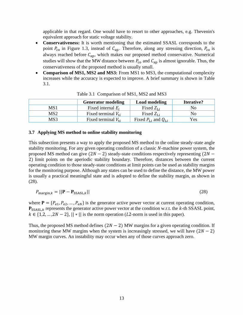
• Comparison of MS1, MS2 and MS3: From MS1 to MS3, the computational complexity
increases while the accuracy is expected to improve. A brief summary is shown in Table
3.1.
Table 3.1 Comparison of MS1, MS2 and MS3
Generator modeling Load modeling Iterative?
MS1 Fixed internal 𝐸𝑖 Fixed 𝑍L𝑖 No
MS2 Fixed terminal 𝑉t𝑖 Fixed 𝑍L𝑖 No
MS3 Fixed terminal 𝑉t𝑖 Fixed 𝑃L𝑖 and 𝑄L𝑖 Yes
3.7 Applying MS method to online stability monitoring
This subsection presents a way to apply the proposed MS method to the online steady-state angle
stability monitoring. For any given operating condition of a classic 𝑁-machine power system, the
proposed MS method can give (2𝑁 − 2) steady-state conditions respectively representing (2𝑁 −2) limit points on the aperiodic stability boundary. Therefore, distances between the current
operating condition to those steady-state conditions at limit points can be used as stability margins
for the monitoring purpose. Although any states can be used to define the distance, the MW power
is usually a practical meaningful state and is adopted to define the stability margin, as shown in
(28).
𝑃margin,𝑘 = ||𝐏 − 𝐏SSASL,𝑘|| (28)
where 𝐏 = {𝑃e1, 𝑃e2, … , 𝑃e𝑁} is the generator active power vector at current operating condition,
𝐏SSASL,𝑘 represents the generator active power vector at the condition w.r.t. the 𝑘-th SSASL point,
𝑘 ∈ {1,2, … ,2𝑁 − 2}, || ∗ || is the norm operation (𝐿2-norm is used in this paper).
Thus, the proposed MS method defines (2𝑁 − 2) MW margins for a given operating condition. If
monitoring these MW margins when the system is increasingly stressed, we will have (2𝑁 − 2) MW margin curves. An instability may occur when any of those curves approach zero.
14
4. Case Studies
4.1 Tests on IEEE 9-bus power system
The IEEE 9-bus power system, whose one-line diagram can be found in [22] and is omitted here,
is selected mainly because it is the smallest multi-machine power system whose steady-state angle
stability boundary can be visualized in a 2-D plot, say 𝑃e2-𝑃e3 space or 𝛿21-𝛿31 space. There are
three machines, therefore, defining two electromechanical modes. Based on the power flow data
from [22], dynamic data from [23] and using classic generator model, the two electromechanical
modes are found to be 1.38Hz and 2.13Hz, where the 1.38Hz mode represents the oscillation
between generator 1 and generators 2 and 3, denoted as mode 1, while the 2.13Hz mode is between
generator 3 and generators 1 and 2, denoted as mode 2.
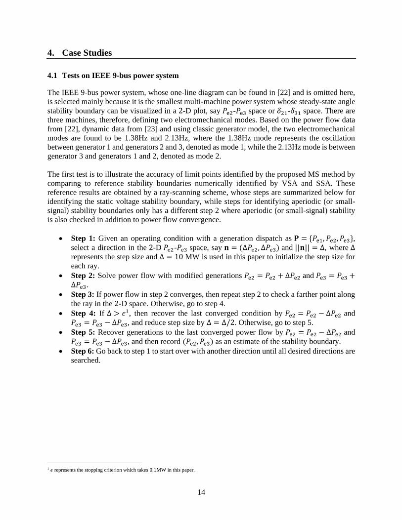
The first test is to illustrate the accuracy of limit points identified by the proposed MS method by
comparing to reference stability boundaries numerically identified by VSA and SSA. These
reference results are obtained by a ray-scanning scheme, whose steps are summarized below for
identifying the static voltage stability boundary, while steps for identifying aperiodic (or small-
signal) stability boundaries only has a different step 2 where aperiodic (or small-signal) stability
is also checked in addition to power flow convergence.
• Step 1: Given an operating condition with a generation dispatch as 𝐏 = {𝑃e1, 𝑃e2, 𝑃e3}, select a direction in the 2-D 𝑃e2-𝑃e3 space, say 𝐧 = (Δ𝑃e2, Δ𝑃e3) and ||𝐧|| = Δ, where Δ
represents the step size and Δ = 10 MW is used in this paper to initialize the step size for
each ray.
• Step 2: Solve power flow with modified generations 𝑃e2 = 𝑃e2 + Δ𝑃e2 and 𝑃e3 = 𝑃e3 +Δ𝑃e3.
• Step 3: If power flow in step 2 converges, then repeat step 2 to check a farther point along
the ray in the 2-D space. Otherwise, go to step 4.
• Step 4: If Δ > 𝜖1, then recover the last converged condition by 𝑃e2 = 𝑃e2 − Δ𝑃e2 and
𝑃e3 = 𝑃e3 − Δ𝑃e3, and reduce step size by Δ = Δ/2. Otherwise, go to step 5.
• Step 5: Recover generations to the last converged power flow by 𝑃e2 = 𝑃e2 − Δ𝑃e2 and
𝑃e3 = 𝑃e3 − Δ𝑃e3, and then record (𝑃e2, 𝑃e3) as an estimate of the stability boundary.
• Step 6: Go back to step 1 to start over with another direction until all desired directions are
searched.
1 𝜖 represents the stopping criterion which takes 0.1MW in this paper.
15
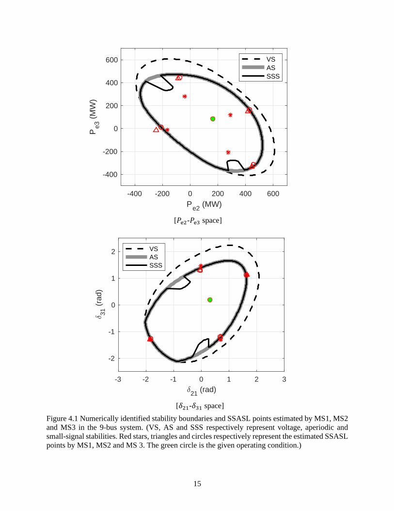
[𝑃e2-𝑃e3 space]
[𝛿21-𝛿31 space]
Figure 4.1 Numerically identified stability boundaries and SSASL points estimated by MS1, MS2
and MS3 in the 9-bus system. (VS, AS and SSS respectively represent voltage, aperiodic and
small-signal stabilities. Red stars, triangles and circles respectively represent the estimated SSASL
points by MS1, MS2 and MS 3. The green circle is the given operating condition.)
-400 -200 0 200 400 600
Pe2
(MW)
-400
-200
0
200
400
600
Pe3 (
MW
)
VS
AS
SSS
-3 -2 -1 0 1 2 3
21 (rad)
-2
-1
0
1
2
31 (
rad
)
VS
AS
SSS

16
Numerically identified reference stability boundaries and the SSASL points estimated by MS1,
MS2 and MS3 are shown in Figure 4.1. Several observations can be obtained: (i) VS boundary is
optimistic in general compared to SSS boundary; (ii) AS boundary mostly coincides with SSS
boundary while is slightly optimistic when self-oscillation instability occurs before an aperiodic
instability; (iii) In 𝛿21-𝛿31 space, SSASL points estimated by MS1, MS2 and MS3 are fairly close
to each other on the AS boundary, showing that all three versions are able to give accurate angle
limit; and (iv) In 𝑃e2 -𝑃e3 space, SSASL points by MS2 and MS3 are fairly close to the AS
boundary while those by MS1 are not quite accurate, though being conservative.
The first test shows how accurate the estimated SSASL points are for a given operating condition
by comparing to reference stability boundaries. In fact, if the actual stressing direction does not
point to any SSASL points, the system will not exit the stability region through one of these SSASL
points estimated at the base-case condition. This is not a problem, since we can always update
these SSASL points by continuously applying the proposed MS method to the most recent system
steady state. To show an online stability monitoring application based on the proposed MS method,
in the second test, the system operating condition is intentionally stressed in a specific direction.
A number of steady states, to be checked by the proposed MS method, are selected between the
base case and the stability limit.
-400 -200 0 200 400 600
Pe2
(MW)
-400
-200
0
200
400
600
Pe3 (
MW
)
VS
AS
SSS

17
Figure 4.2 Estimated SSASL points over stressing.
Figure 4.2 shows the estimated SSASL points over the stressing process where 𝑃e3 increases from
85MW to 414MW (all loads and 𝑃e2 are maintained unchanged) to cause an instability. Five
steady states, from the base case to the limit, are checked by the proposed MS method and the
resulting SSASL points change from red to yellow. Figure 4.2 shows that one of the four SSASL
points, i.e. the one in the first quadrant, arrests the system when it tries to exit the stability region.
It is also observed that when the system gets close to the stability boundary, other SSASL points,
than the one to arrest the system on the boundary, may not be very accurate. This is fine as long
as there is always an SSASL point that accurately arrests the system when it tries to exit the
stability region. This has been found true by exhausting all stressing directions in 𝑃e2-𝑃e3 space
with a small resolution of 2 degrees.
The above visualizes the accuracy of the proposed method and its application in online steady-
state angle stability monitoring. However, such a visualization might not be possible for large
power systems. To this end, the MW margin defined in (28) can help measure and visualize the
distances from an operating condition to SSASL points on the AS boundary. Figure 4.3 shows
these MW margins when applying the proposed approach to multiple steady states over the
stressing process, where the MW margins corresponding to the SSASL point for which the system
is heading are decreasing to zero, while MW margins of other SSASL points are relatively
sufficient, either increasing or staying at 200MW or above.
100 200 300 400 500
Pe2
(MW)
0
100
200
300
400
500
600
Pe3 (
MW
)
VS
AS
SSS

18
Figure 4.3 MW margins v.s. change of 𝑃e3.
4.2 Tests on New England 39-bus power system
This subsection applies the proposed MS method to a large 39-bus power system [24], and two
scenarios are tested. In the first scenario, 𝑃e37 increases and 𝑃e30 decreases by the same MW,
resulting in a stress in the local power transfer and causing a small-signal instability when the
change of 𝑃e37 (or 𝑃e30) reaches 2143.04MW. Along such a stressing direction, the system loses
AS and VS respectively when the change of 𝑃e37 reaches 2142.95MW and 2422.42MW. The
MW margins over stressing are monitored by the proposed method and shown in Figure 4.4, where
MW margins of most SSASL points are above 1000MW even close to the instability while only
two or three SSASL points may encounter low MW margins over stressing. Note that the smallest
MW margin may switch from/to among these two/three SSASL points, as pinpointed in the black
circles, over the stressing process, which calls for the need for monitoring all these critical SSASL
points to not to miss any potential risk. It is also worth mentioning that (i) aperiodic instability and
small-signal instability are extremely close to each other, i.e. less than 0.1MW in the MW change
of the stress, and (ii) right before the system loses it aperiodic stability, the MW margin by (28)
using the voltage stability limit is as huge as 482.68MW, while the MW margins by the proposed
MS method are 54.5MW, 39.79MW and 13.70MW respectively for MS1, MS2 and MS3. Similar
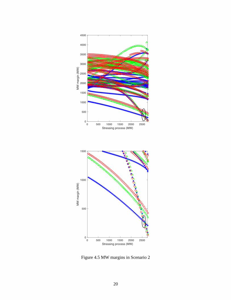
phenomena can also be observed in scenario 2, where 𝑃e33, 𝑃e34, 𝑃e35, 𝑃e36 and 𝑃e38 increase and
𝑃e30, 𝑃e31, 𝑃e32 and 𝑃e37 decrease, stressing the interface between two distantly located generator
groups.
The current implementation of the proposed approach is not efficient, since all derivations are
implemented by Symbolic Math Toolbox in Matlab. In addition, estimating SSASL points
involves the calculation of all eigenvalues and eigenvectors of the linearized system. For a single
operating condition of the 39-bus system, it takes up to 30s. A more efficient implementation
without symbolic derivations, the selection of critical modes for a partial eigen-analysis are our
future work.
0 50 100 150 200 250 300 350
Pe3
-Pe3,basecase
(MW)
0
200
400
600
800
1000
1200P
marg
in (
MW
)MS1
MS2
MS3

19
Figure 4.4 MW margins in Scenario 1
20
Figure 4.5 MW margins in Scenario 2

21
5. Conclusions
This paper proposes a modal-space (MS) method for estimating the steady-state angle stability
limit (SSASL) using the power system nonlinear dynamic model in modal space. The MS method
can estimate the SSASL for all system steady states in a single run. A steady-state angle stability
online monitoring application is developed based on the MS method and tested on the IEEE 9-bus
system and New England 39-bus system. Numerical results show that the proposed MS method is
always able to arrest the system when it tries to exit the aperiodic stability region.
To further show the potential in online environment, dedicated algorithms without symbolic
derivations will be developed to reduce the computation. Future work will also consider N-1
contingency analysis and remedial control actions.

22
References
[1] U.S.-Canada Power System Outage Task Force, “Final report on the august 14, 2003
blackout in the united states and canada: Causes and recommendations,” 2004.
[2] NERC Report, Phase Angle Monitoring: Industry Experience Following the 2011 Pacific
Southwest Outage Recommendation 27, June 2016.
[3] NERC Report, Real-Time Application of Synchrophasors for Improving Reliability, October
2010.
[4] NASPI CRSTT Paper, Using Synchrophasor Data for Phase Angle Monitoring, May 2016.
[5] S. C. Savulescu, Real-Time Stability in Power Systems. New York: Springer, 2014.
[6] T. van Cutsem and C. Vournas, Voltage Stability of Electric Power Systems. Springer US,
1998.
[7] A. Darvishi and I. Dobson, “Threshold-based monitoring of multiple outages with pmu
measurements of area angle,” IEEE Trans. Power Syst., vol. 31, no. 3, pp. 2116–2124, 2016.
[8] H. Yuan, H. Zhang, and Y. Lu, “Virtual bus angle for phase angle monitoring and its
implementation in the western interconnection,” in IEEE PES T&D Conference &
Exposition, pp. 1–5, 2018.
[9] P. Kundur, J. Paserba, V. Ajjarapu, G. Andersson, A. Bose, C. Canizares, N. Hatziargyriou,
D. Hill, A. Stankovic, C. Taylor, T. Van Cutsem, and V. Vittal, “Definition and classification
of power system stability ieee/cigre joint task force on stability terms and definitions,” IEEE
Transactions on Power Systems, vol. 19, pp. 1387–1401, Aug 2004.
[10] S. K. Khaitan, “A survey of high-performance computing approaches in power systems,” in
2016 IEEE Power and Energy Society General Meeting (PESGM), pp. 1–5, July 2016.
[11] H.-D. Chiang and L. F. Alberto, Stability regions of nonlinear dynamical systems: theory,
estimation, and applications. Cambridge University Press, 2015.
[12] P. W. Sauer and M. A. Pai, “Power system steady-state stability and the load-flow
jacobian,” IEEE Transactions on Power Systems, vol. 5, pp. 1374–1383, Nov 1990.
[13] V. A. Venikov, V. A. Stroev, V. I. Idelchick, and V. I. Tarasov, “Estimation of electrical
power system steady-state stability in load flow calculations,” IEEE Transactions on Power
Apparatus and Systems, vol. 94, pp. 1034–1041, May 1975.
[14] Q. F. Zhang, X. Luo, E. Litvinov, N. Dahal, M. Parashar, K. Hay, and D. Wilson,
“Advanced grid event analysis at iso new england using phasorpoint,” in IEEE PES General
Meeting | Conference Exposition, pp. 1–5, July 2014.
[15] F. Saccomanno, Electric Power Systems: Analysis and Control. New York, NY, USA:
Wiley, 2003.
[16] V. Vittal, V. Kliemann, S. K. Starrett, and A. A. Fouad, “Analysis of stressed power systems
using normal forms,” in IEEE International Symposium on Circuits and Systems, pp. 2553–
2556, 1992.
[17] B. Wang, K. Sun, and W. Kang, “Relative and mean motions of multi-machine power
systems in classical model,” arXiv:1706.06226, 2017.
[18] B. Wang, K. Sun, and W. Kang, “Nonlinear modal decoupling of multi-oscillator systems
with applications to power systems,” IEEE Access, vol. 6, pp. 9201–9217, 2018.
[19] B. Wang, K. Sun, and X. Su, “A decoupling based direct method for power system transient
stability analysis,” in IEEE PES GM, pp. 1–5, 2015.
[20] B. Wang, K. Sun, A. D. Rosso, E. Farantatos, and N. Bhatt, “A study on fluctuations in
electromechanical oscillation frequency,” in IEEE PES GM, pp. 1–5, 2014.

23
[21] B. Wang and K. Sun, “Formulation and characterization of power system electromechanical
oscillations,” IEEE Trans. Power Syst., vol. 31, no. 6, pp. 5082–5093, 2016.
[22] P. M. Anderson, Power System Control and Stability. Hoboken: Wiley IEEE Press, 2003.
[23] B. Wang and K. Sun, “Power system differential-algebraic equations,” arXiv:1512.05185,
2015.
[24] T. Athay, R. Podmore, and S. Virmani, “A practical method for the direct analysis of
transient stability,” IEEE Trans. Power App. Syst., vol. PAS-98, pp. 573–584, March 1979.
[25] M. Vaiman, M. Vaiman, S. Maslennikov, E. Litvinov, and X. Luo, “Calculation and
visualization of power system stability margin based on pmu measurements,” in First IEEE
International Conference on Smart Grid Communications, pp. 31–36, Oct 2010.