ANALYSIS STUDY OF THE AXIAL TRANSPORT AND HEAT …
143
ANALYSIS STUDY OF THE AXIAL TRANSPORT AND HEAT TRANSFER OF A FLIGHTED ROTARY DRUM OPERATED AT OPTIMUM LOADING Dissertation zur Erlangung des akademischen Grades Doktoringenieur (Dr.-Ing.) von M.Sc. Mohamed Ahmed Mahmoud Karali geboren am: 01. Dezember 1979 in Kalyobiya, Ägypten genehmigt durch die Fakultät für Verfahrens- und Systemtechnik der Otto-von-Guericke-Universität Magdeburg Gutachter: Prof. Dr.-Ing. Eckehard Specht Institute of Fluid Dynamics and Thermodynamics, Universität Magdeburg, Germany. (Betreuer und Gutachter) JProf. Dr.-Ing. Fabian Herz Institute of Fluid Dynamics and Thermodynamics, Universität Magdeburg, Germany. (Gutachter) Dr.-Ing. Jochen Mellmann Department of post harvest technology, ATB Potsdam, Germany. (Gutachter) Eingereicht am: 07.07.2015 Promotionskolloquium am: 20.08.2015
Transcript of ANALYSIS STUDY OF THE AXIAL TRANSPORT AND HEAT …

ANALYSIS STUDY OF THE AXIAL TRANSPORT AND HEAT TRANSFER OF A FLIGHTED ROTARY DRUM
OPERATED AT OPTIMUM LOADING
Dissertation zur Erlangung des akademischen Grades
Doktoringenieur (Dr.-Ing.)
von M.Sc. Mohamed Ahmed Mahmoud Karali geboren am: 01. Dezember 1979 in Kalyobiya, Ägypten
genehmigt durch die Fakultät für Verfahrens- und Systemtechnik der Otto-von-Guericke-Universität Magdeburg Gutachter:
Prof. Dr.-Ing. Eckehard Specht Institute of Fluid Dynamics and Thermodynamics, Universität Magdeburg, Germany.
(Betreuer und Gutachter)
JProf. Dr.-Ing. Fabian Herz Institute of Fluid Dynamics and Thermodynamics, Universität Magdeburg, Germany.
(Gutachter)
Dr.-Ing. Jochen Mellmann Department of post harvest technology, ATB Potsdam, Germany.
(Gutachter)
Eingereicht am: 07.07.2015
Promotionskolloquium am: 20.08.2015

This work is dedicated to... my father Ahmed, my mother Samia, my wife Alaa and my son Malek

iii
Preface This dissertation is submitted to Otto von Guericke University, Magdeburg for the degree of Doctor of Philosophy. The research described herein was conducted under the supervision of Prof. Eckehard Specht between October 2012 and July 2015. To the best of my knowledge, this work is original, except where suitable references are made to previous works. Neither this, nor any substantially similar dissertation has been submitted for any degree, diploma or qualification at any other university or institution.
Mohamed A. Karali
Magdeburg, 06.07.2015
Think of it as having a wide target selection, where success is a journey; not a destination.

iv

v
Acknowledgements I would like to express my profound gratitude and sincere appreciation to my supervisor Prof. Dr.-Ing. Eckehard Specht for his inspiration, indispensable guidance and for teaching me invaluable knowledge throughout the course of my study. With his initial support, this great dream of mine can finally turn to reality, and with his endless guidance throughout the study, I was able to navigate the arduous path down to the very end. I am sure that whatever I have learned while working with him will be very useful in my future endeavors. He has been a great mentor.
I would like to express my thanks to the reviewers of this work JProf. Dr.-Ing. Fabian Herz and Dr.-Ing. Jochen Mellmann for accepting reviewing my work, providing ideas and text modifications to reshape the current work to be much better. One more time my thanks goes to JProf. Dr.-Ing. Fabian Herz for his continuous encouragement and help during my experimental work in the lab.
I am in deep gratitude to the Future University in Egypt (my main affiliation) for the financial support of my PhD study in Germany. First of all, I should mention Dr. Hassan Azazy the founder of this great establishment. After him I would like to send my thanks and greetings to Mr. Khaled Hassan Azazy, the chairman of the board of trustees of the Future University, for supporting the sending of researchers abroad to complete their studies. Believing in the idea that this kind of cooperation between universities will be beneficial to the Future University and also to our beloved Egypt. I would like to express my deepest gratitude to all people working at the Future University in Egypt. Special thanks to Prof. Dr. Adel Sakr, Prof. Dr.-Ing. Mohamad A. Badr and Prof. Dr.-Ing. Mahmoud Abdelrasheed, for their continued encouragement and valuable advices during all stages in the preparation of this work.
I would like to express my gratitude and thanks to the following people close to me: Herr. Tino Redemann for his continued help and kind, useful discussions. My office-mate Dr.-Ing. Koteswara Rao Sunkara for the useful scientific discussions where his work was a good guide for my PhD. All of our group members for every nice moment spent together, especially Dr.Ing. Janan Al-Karawi, Mr. Ali Mohsan, Mr. Abdelkader Abdelwahab, Mr. Bassam Hallak, Mr. Adnan Tuaamah and Ms. Ainaa Nafsun . My Thanks to our institute secretary Frau. Christin Hasemann for her help with the administrations of my work. Also my thanks goes to all the workers and technicians in the lab, especially to Herr.Timpe for his help and perfect work.

vi
It is my duty to thank the people who worked on the Mathworks - Matlab Center web site (www.mathworks.com) for their great efforts in connecting people searching for solving engineering problems with the most experienced people working in these fields.
I cannot leave without acknowledging all of my Egyptian colleagues in Magdeburg, where without their support and help from the first moment I arrived Germany, It would have been very hard for me to manage my life: Dr.-Ing. Essam Elgendy, Dr.-Ing. Ahmed Hassan and Dr.-Ing. Hassanain Refay. Special thanks from the bottom of my heart to Dr.-Ing. Abouelmagd H. Abdelsamie who helped me with many things including my study.
I am indebted to my parents who grown me up with the good manners that has
credited all the successes in my life. My beloved wife Alaa, she always supported me in the hardest times I encountered during this work. She and my son Malek are the most beautiful things in my life.
Finally, I would like to express my gratitude to everyone who helped me shape the ideas explored in this dissertation, either by giving technical advice or encouraging and supporting my work in many other ways. This dissertation would not have come into existence without their hands-on advice and motivation.

vii
Abstract
The objective of the present work is to study the performance of a flighted rotary
drum operated at optimum loading (design loading). A lot of experiments were carried
out on a 0.5 m diameter and 0.15 m length batch rotary drum furnished internally with
rectangular flights to assess the design loading. Different loadings were examined
through two image analysis methods (manual and automated) of the recorded videos
from under loading to over loading, including design loading. Many solid materials
(free flowing) with different particle diameters and angles of repose, varied rotational
speeds (from 1 to 5 rpm), two numbers of flights (12 and 18), and two flight length
ratios (0.375 and 0.75) were researched. The automated method of the image
analysis showed significant time saving for the extraction process of the data from
the experimental work. However some problems were found when applying the
automated method on the current experimental work images. Indicating that a new
experimental technique should be developed to facilitate both manual and automated
methods. An extension for the experimental work was conducted using a bigger drum
of 1.0 m diameter and 0.3 m length. This extension was based on using a new
experimental technique by modifying the location of both the camera and light. The
discharge characteristics of the drum were studied in order to get information about
the flights holdups, cascading rate and the curtain’s height of fall.
A comparison was conducted between the experimental results and some
available design loading models from literature and a new fitting factor was proposed.
A correlation in terms of the filling degree of design loading conditions and function of
all operating parameters was developed.
A novel mathematical model was proposed to study the axial transport of solids
along the rotary drum using the available experimental results presented in the
current work with the application of a case study. This model is able to predict the

viii
mean residence time of the solid along the drum. The calculated mean residence
time is compared with models available from literature and a new fitting factor was
proposed.
A mathematical model was developed to describe the heat transfer mechanism in
a flighted rotary cooler with application from industry. The results from the heat
transfer model gives information about the temperature profiles of the solid and the
air along the drum. Two approaches were introduced to calculate the heat transfer
area in a flighted rotary drum. New factors for Nusselt correlations of the two
approaches were proposed.
ix
Zusammenfassung
Das Ziel der vorliegenden Arbeit ist die Untersuchung des Verhaltens der
Partikelbewegung in Drehrohren mit rechteckigen Hubschaufeln. Zur Beurteilung
einer optimalen Beladung dieser Hubschaufeln wurden eine Vielzahl von
Experimenten an einer Drehtrommel mit einem Durchmesser von 0.5 m und einer
Länge von 0.15 m durchgeführt. Dabei wurde stets der stationäre Arbeitspunkt der
Partikelbewegung in dieser Drehtrommel betrachtet. Betriebszustände von zu
geringer Beladung, optimaler Beladung bis hin zu einer Überladung der Trommel
wurden untersucht. Die Schüttgutbewegung wurde mit einer hochauflösenden
Kamera aufgezeichnet und mit Hilfe zwei verschiedener Auswertemethoden (manuell
und automatisch) analysiert. Für die Versuche wurden Materialien (trocken und
monodispers) mit unterschiedlichem Partikeldurchmesser und somit verschiedenem
Böschungswinkel verwendet. Dabei wurden die Umdrehungsgeschwindigkeit (von 1
bis 5 U/min), die Anzahl der Hubschaufeln (12 und 18) und das Längenverhältnis der
Hubschaufelkanten (0.375 and 0.75) variiert. Durch die Einführung der
automatischen Auswertemethode des Bildmaterials konnte der Zeitaufwand der
Datenanalyse signifikant reduziert werden.
Der Entleerungsvorgang der Hubschaufeln wurde untersucht, um Aussagen über den
Beladungszustand, die Ausflussrate und die Höhe der Partikelschleier zu erhalten.
Es wurde ein Vergleich angestellt zwischen den erhaltenen experimentellen
Ergebnissen und den verfügbaren Modellen in der Literatur, die den optimalen
Beladungszustand beschreiben. Aufgrund der gewonnen Erkenntnisse wird ein neuer
Anpassungsparameter für die bestehenden Modelle vorgeschlagen. Die Auswirkung
einer Maßstabsvergrößerung auf den Beladungszustand der Hubschaufeln wurde

x
anhand von Versuchen an einer Drehtrommel mit dem Durchmesser von 1.0 m und
einer Länge von 0.3 m untersucht. Dabei konnte das experimentelle Vorgehen so
angepasst werden, dass die manuelle sowie automatische Auswertemethode des
Bildmaterials erleichtert wurde.
Des Weiteren wurde ein mathematisches Modell entwickelt, das den
Wärmeübergangsmechanismus im Drehrohr auf Basis der mittleren Verweilzeit für
das genannte Fallbeispiel beschreibt. Ferner kann dieses Modell zur Vorhersage der
axialen Temperaturprofile des Schüttbettes und der damit in Kontakt stehenden
Gasatmosphäre genutzt werden.

xi
Nomenclature A drum cross section area [m2]
Asur heat transfer surface area (Ch. 6) [m2]
a acceleration [m/s2]
a1 constant in Eq. (5.5)
CD drag coefficient [-]
cp specific heat at constant pressure [kJ/kg⋅K]
cs specific heat of solid material [kJ/kg⋅K]
D drum diameter [m]
dp particle diameter [m]
f filling degree [%]
F force [N]
Fr Froude number, Fr = ω2 R / g [-]
g gravitional acceleration [m/s2]
h solid height of fall [m]
H holdup [m3/m or cm2]
hconv convection heat transfer coefficient (Ch. 6) [W/m3⋅K]
K coefficient in Eq. (5.6)
k coefficient in Eq. (5.8)
k thermal conductivity (Ch. 6) [W/m⋅K]
L drum length [m]
l1 flight radial length [m]
l2 flight tangential length [m]
LMTD Logarithmic temperature difference [oC]
m mass [kg]
N rotational speed [rpm]

xii
nF total number of flights [-]
Nu Nusselt number, Nu = hconv L / k [-]
Pr Prandtl number [-]
Q heat rate [W]
R drum radius [m]
Re Reynolds number [-]
rH effective radial distance of the flight [m]
RMSD root mean square deviation
S gas borne phase to flight borne phase ratio [-]
t time [s]
T temperature [oC]
u velocity [m/s]
Ue overall heat transfer loss coefficient [W/m2⋅K]
Uv volumetric overall heat transfer coefficient between solid and air
[W/m3⋅K]
V drum volume [m3]
x axial position presented in Ch. 6 [m]
X particle axial advance [m]
Y particle falling height [m]
z dimensionless length presented in Ch. 6 [-]
Greek letters
α flight tangential angle [o]
β inclination angle of the drum [o]
γ kinetic angle of repose of solid reside inside the flight [o]
δ flight tip angle [o]
AΘ solid dynamic angle of repose [o] µ dynamic viscosity [m2/s] ρ density [kg/m3] τ mean residence time [s]
ω angular velocity [rad/s]
xiii
Subscripts A angle of repose
a air
avg average
b solid bulk (consolidated)
d drum
design design loading conditions
F flight
FUF first unloading flight
g gas
i directional coordinates implies the flights
L final discharge angle
LUF last unloading flight
p particle
r relative
s solid material
Tot total
x directional coordinates implies the axial direction
y directional coordinates implies falling direction
e heat loss
sa solid-air
sw solid- drum wall
wa drum wall-air

xiv

xv
Contents
Preface iii Acknowledgements v Abstract vii Zusammenfassung ix Nomenclature xi Contents xv
1 Introduction 1 1.1 Granular materials 1
1.2 Granular material flows 2
1.3 Rotary drums 5
1.3.1 Principles 5
1.3.2 Rotary kilns 5
1.3.3 Rotary dryers 7
1.4 Flights 8
1.5 Loading of flighted rotary drums 11
1.6 Thesis outline 16
2 Experimental determination of the optimum loading of a flighted rotary drum
17
2.1 Experimental setup 17
2.1.1 Experimental test rig 17
2.2.2 Experimental procedures 19
2.2.3 Experimental program 20
2.3 Data Processing 21

xvi
2.3.1 Design loading determination criterion 21
2.3.2 Data extraction sequence 21
2.3.3 Image analysis 24
2.3.4 Manual method 26
2.3.5 Automated method 27
2.3.6 Automated method validation 31
2.4 Data fitting 32
2.5 Results and Discussions 32
2.5.1 Influence of number of flights 32
2.5.2 Influence of flight length ratio 35
2.5.3 Influence of Material properties 37
2.5.4 Discharge angle 38
2.6 Comparisons with models from literature 39
3 New experimental technique and scale up 43 3.1 Background 43
3.2 New innovative experimental technique 43
3.3 New experimental work and scaling up the drum size 46
3.4 Results and discussions 48
3.4.1 Influence of number of flights 48
3.4.2 Influence of flight length ratio 50
3.4.3 Comparisons with models from literature 51
3.4.4 Scaling up the drum size 53
3.5 Correlation development 54
4 Determination of the discharge characteristics 57 4.1 Overview 57
4.2 Geometrical parameters 58
4.3 Kinetic angle of repose of the solid residing inside the flight
58
4.4 Flight holdup 63
4.5 Final discharge angle of flight 65
4.6 Flight cascading rate 68
4.7 Curtains height of fall 70
xvii
4.7.1 Measured height of fall 70
4.7.2 Mean height of fall 72
5 Axial transport 75 5.1 Introduction 75
5.2 Physical description of the axial transport in a rotary drum 76
5.3 Models from literature 76
5.3 Current work model description 81
5.3.1 Model assumptions 81
5.3.2 Equationing 81
5.4 Case study 85
5.4.1 Given data 85
5.4.2 Results 86
5.5 Direct application of the model (using in industry) 90
6 Heat transfer 91 6.1 Introduction 91
6.2 Model description 95
6.3 Case study 99
6.3.1 Case study description 99
6.3.2 Results 100
6.4 Defining the heat transfer area 102
6.4.1 First approach (flow over flat plate) 103
6.4.2 Second approach (flow over a spherical particle) 103
6.4.3 New suggested factors for Nusselt correlations 105
7 Conclusions and Outlook 107 7.1 Conclusions 107
7.2 Outlook 109
Bibliography 111
Internet web links 123
List of publications of the current work 124
Curriculum Vitae 125

xviii

1
Chapter 1 Introduction
1.1 Granular materials
A granular material is defined as a collection of discrete macroscopic particles of
sizes larger than 1 µm (Rodhes, 1997, Duran, 1999 and Gennes, 1999). Many basic
products in our daily life including a variety of building materials, chemicals,
pharmaceuticals and food are granular, such as: sand, sugar, corn, wheat, salt,
peanuts, flour, cement, limestone, fertilizers, wood chips, pills etc., see Fig. 1.1 (a).
Although the granular particle is of solid nature it can flows like liquids as the sand do
in an hourglass (see Fig. 1.1 (b)), or when a cereal flows from silos, also it takes the
shape of its container (Menon and Durian, 1997, Kadanoff, 1999, Midi, 2004, Job et al., 2006, Bierwisch, 2009). Thus granular materials can be categorized as a new
form of matter with quit different properties than solids, liquids and gases. Granular
materials are characterized by forming such heaps or piles when resting on a surface
(see Fig. 1.1 (c)), by adding more material the pile will grow until its slope reaches a
critical angle (the critical angle of repose), determined by the size and stickiness of
the grains. Beyond the critical angle, there is some sort of avalanches will happen
(Evesque, 1992, Jaeger and Nagel, 1992 and Frette et al., 1996). Wet sand can be
formed into sandcastles and even, as shown in Fig. 1.1 (d), stable arches. But adding
too much water weakens the sand, so it is no longer can support itself.

2 CH. 1 INTRODUCTION
(a) Examples of granular materials (b) Sand hourglass
(c) Different sand piles (d) Wet sand arches
Figure 1.1: Different granular material characteristics - photos from internet [1].
1.2 Granular material flows
Typical flows of granular materials are illustrated in Fig. 1.2 (Forterre and
Pouliquen, 2008 and Sunkara, 2013). The granular materials flows can be classified
into two categories: the flow confined between two surfaces (Fig. 1.2 (a)-(c)) and the
free surface flows (Fig. 1.2 (d)-(f)). Free surface flows develop a flowing layer on top
of a static bed which is slightly inclined to the horizontal. They have diverse
applications in various industries as well as in the geological practice (Khakhar et al., 2001).

CH. 1 INTRODUCTION 3
Figure 1.2: Typical flows of granular material (a) plane shear, (b) annular shear, (c)
vertical-chute flows, (d) inclined plane, (e) heap flow, (f) rotating drum (Forterre and Pouliquen, 2008 and Sunkara, 2013).
For the flow of granular material in rotating cylinders (rotary drums, will described
in section 1.3) the material is stable till the inclination of the free surface is less than
the dynamic angle of repose (ΘA) (see Fig. 1.3). Increasing beyond this angle leads
to change the stability of the system and a continuous flow of the material is possible
only after the maximum angle of stability. Distinct motion behaviors were identified for
the granular matter in the transverse section of a rotating drum: slipping, slumping,
rolling, cascading, cataracting, and centrifuging (Henein, 1983, Mellmann, 2001,
Mellmann et al., 2001 and Longo and Lamberti, 2002 ). The kind of motion depends
on the nature of the material, drum speed, filling degree, and roughness of the drum
walls. The most common modes of motion behaviors for the industrial rotary drums
are slumping and rolling (Mellmann, 1989, Perron and Bui, 1992, Elperin and Vikhansky, 1998 and Boateng, 1998). During the slumping mode the material
oscillates between two angles, upper and lower angles of repose for every avalanche
(Liu et al., 2005). However, the avalanches are not continuous in this case.
Increasing the drum speed progressively, increases the frequency of avalanches

4 CH. 1 INTRODUCTION which then leads to rolling motion by rolling down the particles continuously. The
surface of the material becomes nearly flat for such motion behavior. This is the
desired mode of operation in the industries for a better performance of the drums.
Due to the fast renewal of the surface the mixing behavior improves. In rotary drums
the filling degree, and the characteristics of the material changes along the length of
the drum. As a result, the rolling and slumping modes occur at different sections of
the drum depending on the filling degree.
Figure 1.3: Transverse motion of a granular material in a rotating drum (Sunkara, 2013).

CH. 1 INTRODUCTION 5 1.3 Rotary drums
1.3.1 Principles
Rotary drums are essential in industry for the manufacturing and the processing
of different granular materials with free flowing or cohesive nature. Rotary kilns,
rotary dryers and rotary coolers are the most commonly used types of rotary drums
within industry. A rotary drum consists of a long cylinder inclined to the horizontal and
have the possibility to rotate around its axis. The solid granular feed is introduced into
the upper end of the drum by various methods including inclined chutes, overhung
screw conveyors and slurry pipes. The charge then travels down along the kiln by
axial and circumferential movements, due to the drum's inclination and rotation.
During the travelling of the solid it interacts with a processing gas along the drum
specially in the gas-borne area for a certain process, in either counter or co- current
flow directions (Friedman and Marshall, 1949), until the processed solid discharged
from the other end of the drum. In the following are more description of the rotary
drums applications.
1.3.2 Rotary kilns
The rotary kiln is one of the most widely used industrial reactors for high
temperature processes (will presented below) involving solids. Thus Its metal cylinder
always lined with bricks or refractory. The kiln inclination depends on the process
with a typical range of values from 1.1o - 3.6o. Different rotational speeds are used
depending on the process and kiln size from very low, i.e., a peripheral speed of 1
rpm, for a TiO2 pigment kiln, to 1.4 rpm for a cement kiln, to 4 rpm for a unit calcining
phosphate material. The sizes of industrial kilns range from 1.7 m (Internal diameter)
x 11.8 m long for firing light weight aggregate, to 5.9 m x 125 m for iron ore direct
reduction. Direct firing or indirect heating may be used, and the kiln can operate in
either co-current or counter-current flow. Solids may be fed either in the dry state, or
as a wet state (Sullivan et al., 1927, Tscheng, 1978 and Henein, 1983 ).

6 CH. 1 INTRODUCTION
The main uses of rotary kilns are in the processes of calcining, fusing, nodulizing,
roasting, incinerating, and reducing of solid materials. Lime, magnesia and alumina
are calcined to release carbon dioxide and water, at temperatures in the ranges of
1260-1500 K. The nodulizing process is applied to phosphate rock and certain iron
ores with temperatures, 1500 to 1600 K. Roasting occurs at temperatures between
800 K and 1600 K, to oxidize and drive off sulfur and arsenic from various ores,
including gold, silver, iron, etc. The rotary kiln is successfully used as a pre-
combustion reactor for incineration of plastics wastes. The temperatures in this
process are in the range of 570-970 K. Iron ore reduction is typical of reducing
processes carried out in rotary kilns. The reaction temperatures are around 1300 K. A
considerable portion of the kiln length may be used to dry solids and bring them up to
reaction temperature. In a typical wet process cement kiln, 60% of the 137 meter kiln
length is required to dry the slurry and heat solids to 1100 K (Tscheng, 1978). An
schematic diagram of a rotary kiln arrangement is shown in Fig. 1.4.
Figure 1.4: Rotary kiln arrangement - photos from internet [2].

CH. 1 INTRODUCTION 7 1.3.3 Rotary dryers
It is worth to define the term drying or dehydration at the beginning, as it refers to
removal of moisture from the matter by evaporation under controlled condition
(Miskell and Marshall, 1965). Some reports suggested that 7-15% of the industrial
energy is concentrated in drying operations for countries like United States, UK,
Canada, and France, whereas countries like Germany, Denmark is further extended
to 15-20% (Raghavan et al., 2005). Since the significance of energy has been rising,
it is necessary to develop the optimal solutions by providing minimum energy
requirements. Drying techniques can be classified as; natural drying or industrial
drying (Smith, 1942 and Van't Land, 1991). Natural Drying, is the oldest method and
most common form of food processing and preservation employed by humankind.
Traditionally, the sun’s energy was used for drying of agricultural and food products.
It is the most widely practiced form of drying in the world because it is cheap, easy,
and convenient. Even though sun drying requires little capital or expertise, there are
many problems in using this method for drying of food products; large space
requirement, long (exposure) drying time, extremely weather dependent, lake of
sufficient control during drying, undesirable changes in the quality of food products,
contamination of the product with soil and dust and non uniformity of drying products.
Whereas the artificial or industrial Drying it overcomes all of the disadvantages of the
natural drying. Nowadays, dryers have an important position in industry for
processing and preservation of different foods and industrial materials. A lot of dryer
types can be found in industry among them, rotary dryers are presented with its
potentials for drying of granular materials.
Rotary dryers are normally employed in the chemical and pharmaceutical
industry, but also are used to dry agricultural products and by - products alfalfa and
beet pulp. i.e; fertilizers, pharmaceuticals, mineral concentrates, cement, sugar,
soybean meal, corn meal, plastics and many others (Williams, 1971, Shirley et al., 1982, Gerhartz, 1985, Savaresi, 2001, Song et al., 2003, Geng et al., 2009 and Abbasfard, 2013). Drying of these by - products and its utilization as animal feed
(cattle), soil conditioner or even as a source of protein is a promising alternative to its
incineration or accumulation in garbage dumps. By its characteristics, this type of
dryers is suitable for the drying of vegetable by - products since it allows the handling

8 CH. 1 INTRODUCTION of heterogeneous or sticky products and products that flow with difficulty. Rotary
dryer is a very complicated process that implies not only thermal drying but also
movement of particles with the dryer.
The direction of the gas flow through the cylinder relative to the solids is dictated
mainly by the properties of the proposed material; Con-current flow is used for heat
sensitive materials even for high inlet gas temperature due to the rapid cooling of the
gas during initial evaporation of surface moisture. Whereas for other materials
counter-current flow is desirable in order to take the advantages of higher thermal
efficiency that can be achieved in this way (Krokida, 2007). Rotary dryers are
classified according to its heating type as: direct, indirect and special types. Direct
heating type (Shene, 1996): heat is added or removed from the solids by direct
exchange between gas and solids (here, heat exchange is by convection and
radiation). such kind of dryers required flights to help for the lifting and showering of
the granular material through the gas-borne area. Also, there should be a perfect
insulation to the dryer shell. Indirect heating type (Kröll, 1978 and Canales, 2001):
the heating medium separated from contact with the solids by a metal wall or tube
(here, heat is dominated by contact heat transfer between the metal wall and solids).
In a special type, Indirect steam tube dryer: one or more rows of steam tubes are
installed longitudinally in its interior, it is suitable for operation up to the available
steam temperature or in process requiring water cooling of the tubes. Typical
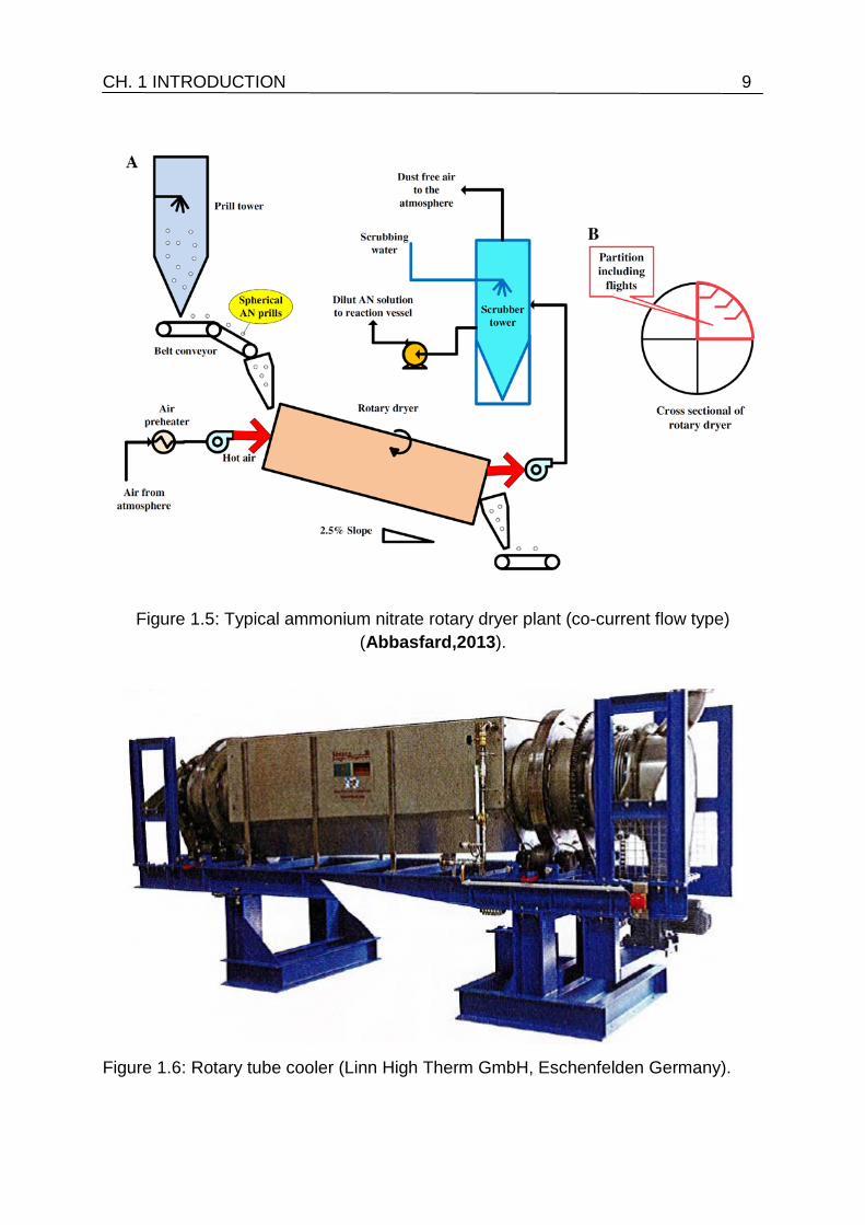
ammonium nitrate rotary dryer plant (Abbasfard,2013) is shown in Fig. 1.5. Rotary
coolers in principle of operation are the same like rotary dryers. Except for the
purpose, here is just focused on cooling the granular material to a certain
temperature using a cold gas stream. Fig. 1.6 shows an industrial rotary tube cooler.
1.4 Flights
Rotary drums interior wall is usually furnished with longitudinal flights
(extended surfaces or fins) as shown in Fig. 1.7, which lifts the granular
material from the bottom bed then cascade and showers it developing a
series of curtains through the gas-borne area (Revol et al., 2001; Krokida
et al., 2007; Lee and Sheehan, 2010; Sunkara et al., 2013a and
Sunkara, 2015).
CH. 1 INTRODUCTION 9
Figure 1.5: Typical ammonium nitrate rotary dryer plant (co-current flow type) (Abbasfard,2013).
Figure 1.6: Rotary tube cooler (Linn High Therm GmbH, Eschenfelden Germany).

10 CH. 1 INTRODUCTION The material falling from the flight is advanced to a specific distance in each cascade
depending on the gas flow type and velocity and various flight actions such as
bouncing and kilning. Due to the inclination of the drum and the action of the flights,
the material is transported to the other end of the drum. The material within the drum
has been exposed to three different phases during the process; the dense phase at
the bottom of the drum, the flight phase (passive), and the gas-borne phase (active)
where the material is exposed to the gas. The effectiveness of the flighted rotary
drum greatly depends on the extent and uniformity of the gas-solid contact and the
residence time of the material in the drum, which in turn depends on the number, size
and shape of the flights. The selection of the shape of the flight is largely governed by
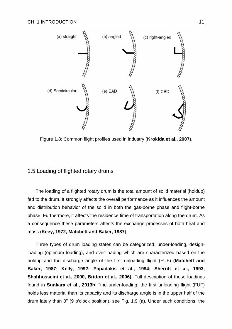
the behavior of flow of the particulates. The most commonly used flight profiles are
shown in Fig. 1.8. In general, rectangular flights are mostly used for free flowing bulk
materials. Radial flights are used for sticky materials and circular flights are
applicable for developing a uniform distribution of the particulates (Moyers, 1997).
Figure 1.7: Cross sectional view of an industrial rotary dryer showing flights (Feeco,
Inc., Wisconsin, USA).
CH. 1 INTRODUCTION 11
Figure 1.8: Common flight profiles used in industry (Krokida et al., 2007).
1.5 Loading of flighted rotary drums
The loading of a flighted rotary drum is the total amount of solid material (holdup)
fed to the drum. It strongly affects the overall performance as it influences the amount
and distribution behavior of the solid in both the gas-borne phase and flight-borne
phase. Furthermore, it affects the residence time of transportation along the drum. As
a consequence these parameters affects the exchange processes of both heat and
mass (Keey, 1972, Matchett and Baker, 1987).
Three types of drum loading states can be categorized: under-loading, design-
loading (optimum loading), and over-loading which are characterized based on the
holdup and the discharge angle of the first unloading flight (FUF) (Matchett and Baker, 1987; Kelly, 1992; Papadakis et al., 1994; Sherritt et al., 1993, Shahhosseini et al., 2000, Britton et al., 2006). Full description of these loadings
found in Sunkara et al., 2013b: ''the under-loading: the first unloading flight (FUF)
holds less material than its capacity and its discharge angle is in the upper half of the
drum lately than 0o (9 o’clock position), see Fig. 1.9 (a). Under such conditions, the

12 CH. 1 INTRODUCTION time spent by the particles in the gas-borne phase is minimum, which can lead to
smaller residence time than required. As the drum loading state is gradually
increased, the FUF position ultimately becomes lower and the unloading starts when
the flight tip is at 9 o’clock position. At this point the drum is said to be at design
loading. In this drum the maximum amount of material is distributed in the gas-borne
phase where the particles total surface area subjected for heat and mass transfers is
substantially increased, hence maximum heat and mass transfers can be expected
between the solids and the gas stream, see Fig. 1.9 (b). Further increasing the feed
rate does not increase the amount of gas-borne solid, but the flights are completely
crowded with the material which is defined as over loading. In this drum the
discharge of the material starts immediately as the flight tip detaches from the bed
surface, see Fig. 1.9 (c) '' .
As a conclusion it is proved that, the best performance of a flighted drum occurs
when the drum operates at design loading conditions (Sheehan et al., 2005, Sunkara et al., 2013b). Therefore, assessing the design-loading of the drum is a
critical issue.
Recently, Ajayi and Sheehan, 2012b carried out an intensive literature survey
about the design loading determination. They performed experimental work on a
horizontal pilot scale rotary dryer with a diameter of 0.75 m and a length of 1.15 m
fitted internally with angular flights. The design load experiments involved two
methods for the image analysis of multiple photographs of the cross sectional area of
the solids in the front end of the dryer at increasing loading conditions. Namely;
manual analysis using ImageJ software and mix of using ImageJ and Matlab image
processing described in Ajayi and Sheehan, 2012a. Subsequently, the design load
was estimated using conventional criteria based on the saturation of material in the
cascading or unloading flights. The proportion of gas-borne to flight-borne solids
within the drum was characterized through a combination of photographic analysis
coupled with Computational Fluid Dynamics (CFD) simulation.

CH. 1 INTRODUCTION 13
Figure 1.9: Experimental photos from Ajayi and Sheehan, 2012b, showing different
drum loading: (a) under loading (b) design loading and (c) over loading.

14 CH. 1 INTRODUCTION
In their work they discussed some available models from literature to calculate
the design loading. They argued that none of those models had been validated
experimentally and most of these models were non-generic and geometrically
developed based on a particular type of flight configurations. Three models were
selected for the comparison with experimental results:- namely the models of Porter (1963), Kelly and O'Donnell (1977) and Baker (1988). Table 1 summarizes the
selected models (Eqs. (1.1) - (1.3)). In addition, they discussed the suitability of using
geometric models of flight unloading to predict design loading in flighted rotary dryers
and they modified Baker’s (1988) model - see Table 1 Eq. (1.4).
Table 1.1: Design loading models
Author Model Porter (1963): 2
FnFUFHTotH ×= (1.1)
Kelly and O'Donnell (1977):
+×=
2
1FnFUFHTotH (1.2)
Baker (1988):
FUFHLUF
FUF iHFlightsTotH −
∑×= 2, (1.3)
Ajayi and Sheehan (2012b):
( )SFUFHLUF
FUF iH.TotH +−∑××=
12241 (1.4)
In Eqs. (1.1), (1.2) and (1.4), HTot is the total holdup of the drum at design
loading including both gas-borne solid (active) and flight-borne solid (passive). HTot,
Flights in Eq. (1.3) represents the total holdup of the drum at design loading accounting
only for the flight-borne solid (passive). In Eqs. (1.1) - (1.4) , HFUF is the holdup of solid
inside the first unloading flight (FUF), and Hi is the holdup in each loaded flight (i) at
design loading starting from the first unloading flight (FUF) to the last unloading flight
(LUF). It should be noted that HTot, HTot, Flights, HFUF and Hi all represent the volumetric
holdup of solid per unit length of the drum. It can be expressed in m3/m (Glikin, 1978)
or in cm2 as presented here in the present work (the frontal cross sectional area of
the solid assuming uniform solid distribution in the axial direction of the drum). nF is
the total number of flights. (S) is the ratio of gas-borne solid to flight-borne solid at
design loading from the experimental work of Ajayi and Sheehan, 2012b and

CH. 1 INTRODUCTION 15 according to their investigated experimental parameters, it has values between
0.042- 0.078. In scaling up the experimental results it is more suitable to use the filling
degree instead of the total mass as the filling degree is a dimensionless parameter.
Eq. (1.5) gives the relation between the drum filling degree and the total solid holdup,
here VTot, solid is the total volume of the solid (total holdup (HTot)) to be fed into the
drum in m3, Vdrum is the total drum volume in m3, R is the radius of the drum (0.25 m)
and L is the length of the drum
1002, ×==
LRπLH
VV
%f Tot
drum
solidTotdesign . (1.5)
It is worth noting that Ajayi and Sheehan, 2012b examined both free flowing and
cohesive solids with cohesion being controlled through the addition of low volatility
fluid with limited range of dynamic angle of repose from 44.7o to 62.3o. The effect of
the drum rotational speed was also examined from 2.5 to 4.5 rpm. Other important
drum design parameters were not examined in their study, like flight length ratio and
number of flights. Changing these design parameters can drastically change the
operation of the drum.
Therefore, in the present work a lot of experiments were carried out to assess the
optimum (design) loading of a batch rotary drum equipped with rectangular (right
angled) flights. Based on the conventional criterion in determining the design loading,
which is the saturation of the FUF with a specific condition where the FUF discharge
angle at 9 o’clock position. The experimental work mainly depends on recording
videos at different operating conditions and then by means of image analysis tools
the results were drawn. Two methods of image analysis were used: manual and
automated. Different solid materials (free flowing), rotational speeds, number of
flights and flight length ratios were researched, each with wide ranges of use and
consequence in industry. The current experimental results were compared with
selected design loading models from literature. Based on the experimental results a
new fitting factor was proposed and a correlation in terms of the total filling degree
was developed. New innovative experimental technique was proposed and used for
more experiments performed on a larger size drum. The discharge characteristics of

16 CH. 1 INTRODUCTION the flighted drum were studied based on the experimental results. Final aim is to
develop a mathematical model describing the axial transport and also the mechanism
of heat transfer along the drum essentially based on using the experimental results in
order to overall evaluate the whole process within the flighted rotary drum.
1.6 Thesis outline
This dissertation is divided into seven chapters. Chapter 2 reports the analysis of
the experimental work carried out in order to assess the optimum loading (design
loading) of a flighted rotary drum (with rectangular flights). Through the description of:
the experimental test-rig, the experimental procedures, different image analysis
techniques used and the results discussions of the design loading. In Chapter 3 the
discharge characteristics of the experimental drum are determined and discussed.
Chapter 4 represents the results of scaling up the experimental drum and developing
a correlation can be used to determine the filling degree at design loading as a
function of all of the operating parameters. Chapter 5 reports the development of a
mathematical model to study the axial transport along the drum using the
experimental results of Chapter 2 with a case study. Chapter 6 is a description for the
heat transfer mechanism of a flighted rotary drum with application of the case study
from Chapter 5. Finally, Chapter 7 reports the conclusions drawn from the present
work and the outlook.

17
Chapter 2 Experimental determination of the optimum loading of a flighted rotary drum
2.1 Experimental setup
2.1.1 Experimental test rig
Figure 2.1 shows the experimental apparatus. The test rig consists of a 0.5 cm
internal diameter and 0.15 m length rotating drum. The drum was directly coupled
with an electrical motor and rotated in the clockwise direction. The rotating speed of
the motor was controlled by a variable frequency inverter. The drum was set up with
zero inclination with respect to the horizontal position on the ground in all directions.
In order to maintain uniform solid distribution inside the drum (that means uniform
axial flight unloading profiles). A line was stretched horizontally in front of the drum
and was located at the center point level of the drum. This line acts as the reference
demarcation between under - loaded and over - loaded condition of the drum (0o
discharge angle at the 9 o’clock position) . Figure 2.2 giving information about the
flight profiles used in the experimental work, which are two rectangular flights of the
same radial length (l1 = 0.05 m ) and two different tangential lengths (l2) of 0.018 m
and 0.037 cm forming two the flight length ratios (l2/l1) 0.375 and 0.75.
18 CH. 2 EXPERIMENTAL DETERMINATION OF THE DESIGN LOADING
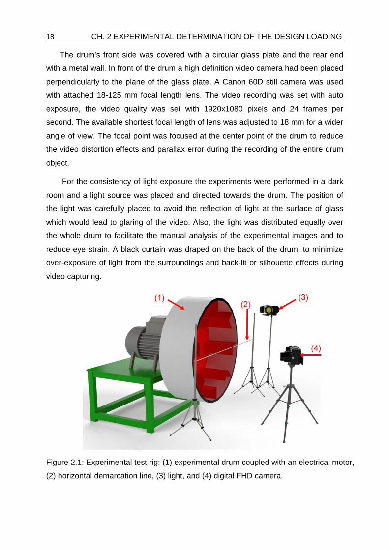
The drum’s front side was covered with a circular glass plate and the rear end
with a metal wall. In front of the drum a high definition video camera had been placed
perpendicularly to the plane of the glass plate. A Canon 60D still camera was used
with attached 18- 125 mm focal length lens. The video recording was set with auto
exposure, the video quality was set with 1920x1080 pixels and 24 frames per
second. The available shortest focal length of lens was adjusted to 18 mm for a wider
angle of view. The focal point was focused at the center point of the drum to reduce
the video distortion effects and parallax error during the recording of the entire drum
object.
For the consistency of light exposure the experiments were performed in a dark
room and a light source was placed and directed towards the drum. The position of
the light was carefully placed to avoid the reflection of light at the surface of glass
which would lead to glaring of the video. Also, the light was distributed equally over
the whole drum to facilitate the manual analysis of the experimental images and to
reduce eye strain. A black curtain was draped on the back of the drum, to minimize
over -exposure of light from the surroundings and back - lit or silhouette effects during
video capturing.
Figure 2.1: Experimental test rig: (1) experimental drum coupled with an electrical motor,
(2) horizontal demarcation line, (3) light, and (4) digital FHD camera.

CH. 2 EXPERIMENTAL DETERMINATION OF THE DESIGN LOADING 19
(a) l2/l1 = 0.75 (b) l2/l1 = 0.375 Figure 2.2: Schematic diagram of the flight geometry used in the experimental work
(rectangular flight l2 (tangential length) and l1 (radial length) = 0.05 m).
2.2.2 Experimental procedures
The experimental procedure after the preparation of experimental setup was as
follows: the amount of solid was determined according to the experimental design in
terms of drum filling degree and filled into the drum. For example, at a certain desired
filling degree the solid holdup (volume VTot, solid in m3) was calculated from Eq. (1.5)
where Vdrum is the total drum volume. The calculated solid volume was converted to
mass (in kg) using the solid bulk density (measured in laboratory, the solid was
weighed for five samples with different volumes and the density was calculated as
the mean value). Then weighing out this specified mass of the solid and filling it into
the drum. The same procedure was used for incrementing the solid filling degree. As
in most cases, the drum filling degree was firstly increased at regular intervals by 1%
with respect to the previous reading. When the drum was found to be close to the
design loading point (where the FUF discharge angle was nearly at 9 o’clock
position), the experiments were repeated before and after this point by small
increments of filling degree (depending on experience). Until the design loading point
was more precisely determined. With this in mind, some points in between were
added to ensure the reliability of the results. The motor was provided with electricity
and the frequency control was manipulated to obtain the desired drum rotational
speed. After switching on the motor a moment was waited until the material was fully
distributed in the drum and a video was recorded for approximately two minutes.
Then the motor was stopped for the next experiment with the new filling degree.
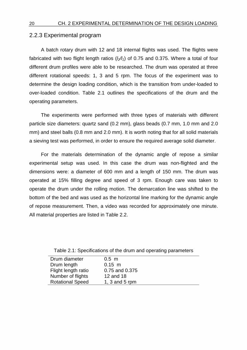
20 CH. 2 EXPERIMENTAL DETERMINATION OF THE DESIGN LOADING 2.2.3 Experimental program
A batch rotary drum with 12 and 18 internal flights was used. The flights were
fabricated with two flight length ratios (l2/l1) of 0.75 and 0.375. Where a total of four
different drum profiles were able to be researched. The drum was operated at three
different rotational speeds: 1, 3 and 5 rpm. The focus of the experiment was to
determine the design loading condition, which is the transition from under-loaded to
over-loaded condition. Table 2.1 outlines the specifications of the drum and the
operating parameters.
The experiments were performed with three types of materials with different
particle size diameters: quartz sand (0.2 mm), glass beads ( 0.7 mm, 1.0 mm and 2.0
mm) and steel balls (0.8 mm and 2.0 mm). It is worth noting that for all solid materials
a sieving test was performed, in order to ensure the required average solid diameter.
For the materials determination of the dynamic angle of repose a similar
experimental setup was used. In this case the drum was non-flighted and the
dimensions were: a diameter of 600 mm and a length of 150 mm. The drum was
operated at 15% filling degree and speed of 3 rpm. Enough care was taken to
operate the drum under the rolling motion. The demarcation line was shifted to the
bottom of the bed and was used as the horizontal line marking for the dynamic angle
of repose measurement. Then, a video was recorded for approximately one minute.
All material properties are listed in Table 2.2.
Table 2.1: Specifications of the drum and operating parameters
Drum diameter 0.5 m Drum length 0.15 m Flight length ratio 0.75 and 0.375 Number of flights 12 and 18 Rotational Speed 1, 3 and 5 rpm

CH. 2 EXPERIMENTAL DETERMINATION OF THE DESIGN LOADING 21
Table 2.2: Physical properties of materials
Material dp
(mm)
ρb (consolidated)
(kg/m3)
ΘA
(o)
Quartz sand 0.2 1570 ±18 32.4 ±1.1 Glass beads 0.7 1560 ±20 28.0 ±0.6
1.0 1555 ±22 25.9 ±0.8 2.0 1549 ±15 25.7 ±1.0
Steel balls 0.8 4630 ±25 28.5 ±0.9 2.0 4680 ±27 25.5 ±0.7
2.3 Data Processing
2.3.1 Design loading determination criterion
The determination of the design loading filling degree from the experimental
results was based on two observations from the recorded videos and images
analysis processing. First, that the FUF starts to cascade (discharge) the solid at 9
o’clock position; Second, that the cross sectional area of the first unloading flight
(FUF) attained a maximum value or saturation. Figs. 2.3 and 2.4 illustrates samples
from the current experimental work at different operating conditions, showing different
loadings of the flighted rotary drum including the design loading (see cases (b)).
2.3.2 Data extraction sequence
The sequence of data extraction was as the following: at first the video was
recorded during the experiment with a specific material, rotational speed, number of
flights, flight length ratio and filling degree of the drum. Then, the video was
segmentized using VLan Player and still images of interest were extracted from the
video. Those still images of the first unloading flight were selected and compared
side by side in terms of image clarity and positioning of the discharge angle. At least
ten images were selected for each operating condition. These selected still images
were to be analyzed using a suitable software in order to calculate the FUF area and
other parameters as will described in the followings.

22 CH. 2 EXPERIMENTAL DETERMINATION OF THE DESIGN LOADING
(a)
(b)
(c)
nF 12 nF 18
Figure 2.3: Sample photos from our experimental work showing different loadings,
dashed circle denoted the FUF; (a) under loading (b) optimum design loading and (c)
over loading. For two number of flights 12 and 18.
9 o'clock (0o) position

CH. 2 EXPERIMENTAL DETERMINATION OF THE DESIGN LOADING 23
(a)
(b)
(c)
l2/l1 0.375 l2/l1 0.75
Figure 2.4: Sample photos from our experimental work showing different loadings, for
two flight length ratios 0.375 and 0.75.
9 o'clock (0o) position

24 CH. 2 EXPERIMENTAL DETERMINATION OF THE DESIGN LOADING 2.3.3 Image analysis
Image analysis is a powerful tool for solving different engineering problems in
particle technology. It is the process of extracting important information from the
image; mainly from digital images by means of digital image processing techniques.
Most of the scientific publications using the image analysis have been arisen from the
biological science fields with application of measuring size and counting the number
of bacteria in an image. MASSANA, et al., 1997, compared two methods for
measuring size and counting the number of Planktonic bacteria represented in
different water bodies samples as shown in Fig. 2.5. The first method was by the
direct counts, the second was based on computerized image-analysis of
epifluorescence preparations, they concluded that the computerized method was the
most accurate and simple method to be used. Heffels, et al., 1996, studied different
possibilities of changing backward light scattering for characterizing dense particle
systems. Obadiat, et al., 1998, developed an innovative digital image analysis
approach to quantify the percentages of voids in mineral aggregates of bituminous
mixtures.
Figure 2.5: Whole process of image processing by Massana, et al., 1997, process
from the original image to the final binary image. For counting Planktonic bacteria
represented in a water body.

CH. 2 EXPERIMENTAL DETERMINATION OF THE DESIGN LOADING 25
The digital image to be analyzed can be defined as a two dimensional array of x
and y, where x and y are plane coordinates. A pixel is the smallest element of an
image represented on the screen. The address of a pixel corresponds to its physical
coordinates (x, y). The total number of pixels in an image depending on: the device
(the camera) used for capturing the digital image or the video where the image is
drawn from and the size of the image. There are four basic types of images which
can be defined namely:- red- green-blue (RGB or true color) image, indexed image,
gray scale image and binary (black and white) image.
In the RGB image each pixel has a color which is described by the amounts of
red, green, and blue in it. Each of these components can have a range of values from
0 to 255 giving a total of 2553 = 16,581,375 different color possibilities in the image
and each pixel in an image corresponds to three values. This leads to deal with a
complicated analysis process. The indexed image likes a color map and each pixel
with a value does not give its color but an index to its color in the color map. The gray
scale image is characterized by shades of gray and the pixel ranges from 0 for black
and 255 for white. In the binary image (black and white image) the pixels are either
black with value of 0 or white with value of 1. The image analysis technique is much
influenced by the type of image to be processed. Where complicated analysis
technique is needed for the true color images. The technique becomes easier when
using gray scale images and more easier when using binary (black and white)
images. Thus, gray scale and binary (black and white) images are predominantly
used in image analysis for engineering applications.
Previous studies on rotary drums have used different image analysis methods.
As for the studies of particles mixing in rotary drums: Van Puyvelde, 1999, describes
a new way to determine the mixing rates of solids in a rotating drum through image
analysis programming using custom software written in Borland C ++. Recently, Liu et al., 2015, conducted a quantitative comparison of image analysis methods
namely:- pixel classification, variance method and contact method for studying
particle mixing in rotary drums using the image processing toolbox provided by
Matlab. Whereas for the studies of rotary drums loading (holdup) and curtains
behavior : ImageJ software was used for the image analysis processing by Lee and Sheehan, 2010 and Ajayi and Sheehan, 2012a. Moreover Ajayi and Sheehan,

26 CH. 2 EXPERIMENTAL DETERMINATION OF THE DESIGN LOADING 2012a, have used another method which is a combination of ImageJ software and
Matlab image processing toolbox.
In the present experimental work, two methods were introduced and compared
for the image analysis processing: first, manual method (mainly using ImageJ
software); second, automated method (by using a combination of ImageJ software
and Matlab image processing toolbox). In the following a full description of the two
methods.
2.3.4 Manual method
In the manual method ImageJ software was used. The first process was the
scaling of the image, which means identifying a reference length like using the
diameter of the drum (50 cm). Then manually selecting the area of interest (like the
material reside in a flight). Special care was taken to avoid errors in selection. A
multipoint polygon selection was used in order to have an accurate selection of the
material without selecting the drum metal parts. Another problem appeared was the
difficulty in identifying the separating edges between the material frontal cross section
area and its side view (see Fig. 2.6). That leaded to high time consumption and error
probability. After selecting the area of interest ImageJ measured the area in cm2 by
counting the number of pixels relying on the predefined scaling factor. Then one by
one all the areas of solid materials in all flights were measured.
Another study will depend on measuring the variation of the material frontal cross
section area with the change in the discharge angle, in such case the video will be
running and by choosing one flight to be traced from the FUF position to the LUF
position and captured many images at different positions (different discharge angles,
also can be measured by ImageJ). The same processes as mentioned before can be
applied to measure the curtains falling height.
As a conclusion, the manual method resulting in significant time consumption
which became the major limitation of this image analysis processing method. And it is
better to find an automated method to save the significant time consumption.

CH. 2 EXPERIMENTAL DETERMINATION OF THE DESIGN LOADING 27
Figure 2.6: Manual selection of solid material reside in the flights.
2.3.5 Automated method
The automated method mainly was developed to overcome the disadvantages of
the manual method, to save the significant time consumption especially for the
analysis of numerous images. The automated method relied on using a combination
of ImageJ software and Matlab image processing toolbox. The ImageJ software was
used for the pre-processing (enhancement) of the images and then Matlab was used
to find all of the required information.
Matlab image process toolbox can read and threshold colors from all images
types. The reading process results in giving information about the total number of
pixels represented in a specified region for a specified color. In order to simplify the
engineering problem (threshold process) the type of image choosed to be analyzed is
the binary (black and white) one. The images of the current experimental work were
of true color type. Thus it was first transformed to binary type. But it could not be
transformed directly due to many problems. First, the appearance of the material’s
side view in the flight. Second, the existence of the curtains formed by the material
cascaded from the upper loaded flights. As these curtains are of the same color as
the materials reside in the flights. That leads to a wrong fuzzy selection by imageJ.
Third, the lighting intensity (brightness) of the image was horrible for the
transformation (this light was settled to make convenience for the manual analysis).

28 CH. 2 EXPERIMENTAL DETERMINATION OF THE DESIGN LOADING Fourth, there were a large number of images to be pre-processed before analyzed by
Matlab which resulted in more time consuming as the manual method. To overcome
all of the mentioned problems a Macro code was developed in the ImageJ software
for the batch pre-processing of unlimited number of images. But before using this
Macro code, the side view’s of the material reside inside the flights were to be
removed by manual selection (this was only for the current experimental images, but
it is recommended in future to extend the experimental work with new technique in
avoiding the appearance of the material’s side views). The Macro processes were
first, the image was cropped to the inner diameter of the drum in order to make all
images with the same size. Second, the part where the curtains exist were removed
by choosing the inner circle passing by the end point of the tangential length of all
flights). Third, the brightness and contrast was adjusted using the built-in function by
the ImageJ (depend on the already exist one). Fourth, the true color images were
transformed to be in gray scale and then binary (black and white) as shown in Fig. 2.7.
A Matlab code was developed to calculate the total number of white pixels (of the
solid) reside in each flight (in a specified region selected by using the function
“roipoly” with a special care to avoid the selection of some metal parts of the drum).
In order to calculate the actual area of these regions, the total number of the pixels in
the whole image (which means with known area of the drum inner diameter circle)
was counted first and by normalizing the number of pixels of the selected regions
with the total image the area could be calculated. Unlimited number of images can be
analyzed with this methodology for any study.

CH. 2 EXPERIMENTAL DETERMINATION OF THE DESIGN LOADING 29
(a) Original image
(b) After removing side views and
cropping to the inner diameter
(c) After brightness and contrast
adjustment
(d) Image in gray scale
(e) Final black and white (BW) image to Matlab
Figure 2.7: Pre-processes of the experimental raw photo using ImageJ.

30 CH. 2 EXPERIMENTAL DETERMINATION OF THE DESIGN LOADING
a) Original image example b) Filtered image example
Figure 2.8: Experimental images from Ajay and Sheehan, 2012a.
Ajay and Sheehan, 2012a used similar image analysis technique, as the
original image taken by the camera was in grayscale and the camera location was
focused at the 9 o’clock position (FUF). But they added some more pre-processes for
the images before feeding to Matlab, like using some filters to enable the selection of
the material curtains in the air-borne area as well as the material reside in the flights
as shown in Fig. 2.8. But on contrary, through the text of their publication they argued
the fact that in order to estimate the area of the material reside in the flight, the air-
borne area should be removed from the image. Also, they argued that the camera
location led to unavoidable difficulties determining the edges of the flight born solids,
that makes the use of the naked eye in determining the edges (manually) is more
reliable but strainfull.
As a conclusion, the automated method (using combination of ImageJ software
and Matlab image processing toolbox) is much time saving for the calculations. But
the camera location and lighting location, angle and intensity should be adapted in
order to avoid the appearance of the material’s side views and also to avoid any
reflections on the drum frontal cover glass. That way, the transformations of the true
color images (RGB) to the binary (black and white) one will be much easier and does
not need much manual processes. Also it should be mentioned that, in order to get

CH. 2 EXPERIMENTAL DETERMINATION OF THE DESIGN LOADING 31
effective use from the automated method (decrease the processing time), the camera
location and lighting location, angle and intensity should be the same for all the
captured videos of the experimental work. As the batch cropping process will be
much easier and precisely. Hence, it is recommended to develop a new experimental
technique in future to overcome all the mentioned problems and facilitate both
manual and automated methods, as will be described in Ch. 3.
2.3.6 Automated method validation
A comparison was conducted between the manual and the automated methods
in order to validate the use of the automated method (Matlab code). The comparison
is based on calculating the FUF cross sectional area (or holdup HFUF in cm2) at the
same conditions (only at design loading) using both manual and automated methods
(the determination of the design loading points were described later). The
comparisons revealed a good matching between both methods for all cases with
small error of +3.2% RMSD represented by the shaded area as shown in Fig. 2.9.
Figure 2.9: Comparison between manual and automated methods based on calculating
the HFUF at the design loading conditions. the shaded area represents the RMSD.
14 16 18 20 22 24 26 28HFUF Manual calculation in cm2
14
16
18
20
22
24
26
28
HFU
F A
utom
ated
cal
cula
tion
in c
m2

32 CH. 2 EXPERIMENTAL DETERMINATION OF THE DESIGN LOADING 2.4 Data fitting
In the regression of the experimental data set a simple linear fitting was used.
The data set splitted into two groups with breaks in location at the estimated design
loading point. These break points were firstly determined by the direct vision as
almost all of flights are saturated and starts its cascading when reaching precisely the
9 o’clock position. Then by means of image analysis and calculations of the FUF area
over the filling degree these points were verified. After the predetermination of the
design loading point filling degree the calculation of the FUF area was focused only
at the 9 o’clock position. Otherwise any increase in the filling degree would have
caused a case of overloading and introduced a higher FUF area at a lower discharge
angle than the 0o. The left side of the break points was fitted linearly with an
increasing slope of the HFUF, while the right side of the break points was fitted linearly
with zero inclination as the HFUF is remains almost constant here.
The measured average FUF cross sectional area is plotted versus the drum
filling degree in the following Figures. 2.5 Results and Discussions
2.5.1 Influence of number of flights Figure 2.10 shows the influence of the drum filling degree on the measured FUF
cross sectional area for rotational speeds of 1, 3 and 5 rpm and the number of flights
12 and 18. It is clearly shown that at any rotational speed an increasing filling degree
causes the FUF cross sectional area to increase until it becomes saturated. The point
of saturation is considered as the design loading point. It is characterized by a FUF
discharge angle at the 9 o’clock position. This is due to the increase of the holdup
carried by the flights. For the same number of flights, increasing the rotational speed
leads to shift the point of saturation (design loading point) in the direction of an
increasing filling degree. Which means higher filling degree is required for the design
loading point. This can be attributed to the increased rate of discharge of solid into
the gas-borne phase. That requires more material adding to substitute the saturation
of the FUF at design loading (see Fig. 2.11). This is further supported by the
observed decrease in the slope of the area versus the filling degree line. It is also

CH. 2 EXPERIMENTAL DETERMINATION OF THE DESIGN LOADING 33
shown from Fig. 2.10 increasing the number of flights at the same rotational speed
increases the design loading filling degree, this is related to the increase of the total
holdup (see Fig. 2.11).
From Fig. 2.10 (a) for quartz sand it can be noted that the saturation (maximum)
value of the measured FUF cross sectional area are in the range of 26 cm2. For the
12 flights drum the increase in the rotational speed from 1 to 5 rpm causes an
increase in the required design loading filling degree from 8.7 to 10%, respectively,
which is an increase of 14.9%. For the drum of 18 flights that increase is from 12.7 to
14.8%, a 16.5% increase in the design loading filling degree. By comparing the
values of the filling degree required for the design loading points of the 12 flights
drum to the 18 flights drum an average increase of 46.5% can be observed.
Figure 2.10 (b) for glass beads shows comparable values of the FUF cross
sectional area in the range of 25 cm2. For the 12 flights, drum the required filling
degree for design loading increased from 8.5 to 10.1% when the rotational speed
increased from 1 to 5 rpm, an increase of 18.8%. For the drum with 18 flights, the
filling degree varied from 12.8 to 14.7%, which is an increase by 14.8%. In order to
achieve design loading conditions using 18 flights, on average 48.1% more material
needed to be added when compared with the amount of material used by the 12
flights drum for the same design loading conditions.
From Fig. 2.10 (c) for steel balls it is seen that there are comparable values of
the FUF cross sectional area in the range of 25 cm2. For the 12 flights drum, the
increase in the rotational speed from 1 to 5 rpm caused an increase in the required
design loading filling degree from 9.1 to 10.2%, an increase of 12%. For the drum
with 18 flights the increase was from 13 to 14.7%, which is a 13% increase. In
comparing the values of the filling degree required for the design loading points of the
12 flights drum to the 18 flights drum an average increase of 41.6% was observed.

34 CH. 2 EXPERIMENTAL DETERMINATION OF THE DESIGN LOADING
Figure 2.10: Measured FUF cross sectional area versus drum filling degree for
various rotational speeds and number of flights (a) quartz sand (b) glass beads (c)
steel balls.
6 7 8 9 10 11 12 13 14 15 160
5
10
15
20
25
30
HFU
F in
cm
2
quartz sanddp 0.2 mmΘA 32.4o
ρb 1570 kg/m3
nF 12 nF 18
1 rpm3 rpm5 rpm
(a)
l2/l1 0.75
D 0.5 mL 0.15 m
6 7 8 9 10 11 12 13 14 15 160
5
10
15
20
25
30
HFU
F in
cm
2
glass beadsdp 0.7 mmΘA 28.0o
ρb 1560 kg/m3
nF 12 nF 18
1 rpm3 rpm5 rpm
(b)
l2/l1 0.75
D 0.5 mL 0.15 m
6 7 8 9 10 11 12 13 14 15 16fD in %
0
5
10
15
20
25
30
HFU
F in
cm
2
steel ballsdp 0.8 mmΘA 28.5o
ρb 4630 kg/m3
nF 12 nF 18
1 rpm3 rpm5 rpm
(c)
l2/l1 0.75
D 0.5 mL 0.15 m

CH. 2 EXPERIMENTAL DETERMINATION OF THE DESIGN LOADING 35
Figure 2.11: Measured design loading filling degree in denpendence of rpm for
various materials, at two number of flights of 12 and 18 and flight length ratio of
0.75.
2.5.2 Influence of flight length ratio
Figure 2.12 illustrates the variation of the measured FUF cross sectional area
versus the drum filling degree for various rotational speeds from 1 to 5 rpm and two
flight length ratios of 0.375 and 0.75. It can be seen that increasing the flight length
ratio caused an increase in both the FUF cross sectional area and the filling degree
required for the design loading point. This is because of the increase of the individual
flight holdup and eventually the total holdup. Therefore, flighted rotary drums with
longer flight tangential length requires more drum filling degree to reach design
loading condition compared to rotary drums with shorter flight tangential length (see
Fig. 2.13). Figure 2.12 (a) for glass beads with particle diameter of 0.7 mm showed an
increase in the average measured FUF cross sectional area from 15 to 26 cm2 on
average while changing the flight length ratio from 0.375 to 0.75 resulted in a
percentage increase of 73.3. At a flight length ratio of 0.375 the required drum filling
degree for the design point increased from 4.8 to 5.8% when the rpm changes from 1
to 5 which is an increase of 20%. For the flight length ratio of 0.75 an increase was
observed from 8.5 to 10.1%, which is a percentage increase of 18.8. Comparing the
results of the two flight length ratios it can be seen that the required drum filling
degree for the design loading increases by an average of 75.5%.
1 2 3 4 5
rpm
8
9
10
11
12
13
14
15
f D in
%
l2/l1 0.75
D 0.5 mL 0.15 m
nF 12nF 18
quartz sand dp 0.2 mmglass beads dp 0.7 mmsteel balls dp 0.8 mm

36 CH. 2 EXPERIMENTAL DETERMINATION OF THE DESIGN LOADING In Fig. 2.12 (b) for glass beads with particle diameter of 1.0 mm showed an increase
in the average measured FUF cross sectional area from 16 to 22.5 cm2 while
changing the flight length ratio from 0.375 to 0.75 which is a percentage increase of
40.6. At the flight length ratio of 0.375 the required drum filling degree for the design
loading point changed from 4.5 to 5.5% when the rpm changes from 1 to 5, which is
an increase of 22.2%. For the flight length ratio of 0.75 an increase was observed
from 8.1 to 9.4%, which is a percentage increase of 16. Comparing the results of the
two flight length ratios it can be seen that the required drum filling degree for the
design loading condition increased on average by 77%.
Figure 2.12: Measured FUF cross sectional area versus drum filling degree for
various rotational speeds and flight length ratios (a) glass beads 0.7mm (b) glass
beads 1.0mm.
2 3 4 5 6 7 8 9 10 11 120
5
10
15
20
25
30
HFU
F in
cm
2
glass beadsdp 0.7 mmΘA 28.0o
ρb 1560 kg/m3
l2/l1 0.375
l2/l1 0.75 (a)1 rpm3 rpm5 rpm
nF 12
D 0.5 mL 0.15 m
2 3 4 5 6 7 8 9 10 11 12fD in %
0
5
10
15
20
25
30
HFU
F in
cm
2
l2/l1 0.375
l2/l1 0.751 rpm3 rpm5 rpm
glass beadsdp 1.0 mmΘA 25.9o
ρb 1555 kg/m3
(b)
nF 12
D 0.5 mL 0.15 m

CH. 2 EXPERIMENTAL DETERMINATION OF THE DESIGN LOADING 37
Figure 2.13: Measured design loading filling degree in dependence of rpm for
various materials, at two number of flights of 12 and 18 and flight length ratio of
0.75.
2.5.3 Influence of Material properties
Figure 2.13 depicts the variations of the measured FUF cross sectional area
versus the drum filling degree for different material properties (particle diameter and
dynamic angle of repose). In Fig. 2.13 (a) it is shown that comparable values of FUF
cross sectional area is attained of about 25 cm2. Also, it can be noted that the design
loading filling degree needed for glass beads of 0.7 mm particle diameter and 28o
angle of repose is comparable to the one needed for glass beads of 2.0 mm particle
diameter and 25.7o angle of repose within a range of 9%.
It can be understood from Fig. 2.13 (b) that the needed filling degree for steel balls of
0.8 mm particle diameter and 28.5o angle of repose is 10%. While the one needed for
steel balls of 2.0 mm and 25.5o angle of repose is 9% which is a 11.1% difference.
Comparable values of the FUF cross sectional area were attained with a average of
24.5 cm2. These unexpected observations maybe related to the error in measuring
the dynamic angle of repose.
1 2 3 4 5
rpm
4
5
6
7
8
9
10
11
f D in
%
nF 12l2/l1 0.375l2/l1 0.75
D 0.5 mL 0.15 m
glass beads dp 0.7 mmglass beads dp 1.0 mm

38 CH. 2 EXPERIMENTAL DETERMINATION OF THE DESIGN LOADING
Figure 2.13: Measured FUF cross sectional area versus drum filling degree for
various material particle diameters and dynamic angles of repose (a) glass beads
(b) steel balls.
2.5.4 Discharge angle
For better understanding of the influence of the drum filling degree on the FUF
discharge angle (discussed before in Ch. 1); an example from the experimental
results for quartz sand at different rotational speeds is illustrated in Fig. 2.14. As
shown from Fig. 2.14 at any rpm (i.e. 1 rpm) an increasing drum filling degree (from
the under-loading to the over-loading) leads to lower the FUF discharge angle until it
becomes at the 9 o’clock (see Fig. 1). This point considered the design loading of the
drum and the corresponding value of the filling degree as shown before in Fig. 2.10 is
8.7%.
6 7 8 9 10 11 120
5
10
15
20
25
30
HFU
F in
cm
2
nF 12l2/l1 0.75n 3 rpm
0.7 mm1.0 mm2.0 mm
ΘA 28.0o
ΘA 25.7oΘA 25.9o
(a)
glass beads
D 0.5 mL 0.15 m
6 7 8 9 10 11 12fD in %
0
5
10
15
20
25
30
HFU
F in
cm
2
nF 12l2/l1 0.75n 3 rpm
0.8 mm2.0 mm
ΘA 25.5o
ΘA 28.5o
(b)
steel balls
D 0.5 mL 0.15 m

CH. 2 EXPERIMENTAL DETERMINATION OF THE DESIGN LOADING 39
Figure 2.14: FUF discharge angle versus drum filling degree for quartz sand at three
rotational speeds.
2.6 Comparisons with models from literature
Table 2.3 outlines the experimental results for different operating conditions, the
design loading filling degree and the FUF cross sectional area at the design loading
point. The average slandered deviation in measuring the FUF area only at design
loading points is also listed in Table 2.3.
Comparisons between the experimental results and some available models
from literature (Porter, 1963; Kelly and O'Donnell, 1977 and Ajayi and Sheehan, 2012b (modified Baker’s model)) were conducted and shown also in Table 2.3. Ajayi and Sheehan 2012b showed that the S factor values in Eq. (1.4) are small, with a
typical range of 0.042- 0.078. Due to this, the term in Eq. (1.4) including the factor S
was neglected in the present work. Consequently the comparison of the current
experimental results with the mentioned models will be based on flight-borne data
only, as HFUF and Hi were extracted from the photos and used directly in the models.
Then the resulted HTot from the models were converted to filling degree using Eq.
(1.5) and finally were compared with one of the current experimental results. The
comparisons revealed that no model was able to describe the design loading
precisely. The one developed by Ajayi and Sheehan, 2012b yields the lowest
deviation, especially at lower rotational speeds (10-15%). Based on our experimental
6 7 8 9 10 11 12fD in %
0
10
20
30
40
50
60
70
80
90
Dis
char
ge a
ngle
at F
UF
in o
1 rpm3 rpm5 rpm
quartz sanddp 0.2 mmΘA 32.4o
ρb 1570 kg/m3
nF 12l2/l1 0.75
D 0.5 mL 0.15 m

40 CH. 2 EXPERIMENTAL DETERMINATION OF THE DESIGN LOADING data, the new fitting factor 1.38 can be proposed to modify Baker’s model, 1988 to
give the best fit (when using rectangular flights) as shown in Eq. (2.1).
Present work, model for design loading: FUFH
LUF
FUF iH.TotH −
∑××= 2381 (2.1)
Based on the experimental results, it can be suggested that to ensure optimum
(design) loading of a rotary drum, the volume occupied by the solid should be
between 5-15% of the total drum volume. The range reported by Perry and Green,1999 was 10-15%. The reason behind the difference between the two ranges
is that the present work studied the influence of the flight length ratio, where the
smaller flight length ratio (0.375) reveals that 5% filling degree is required for
optimum loading.
Table 2.3: Experimental results and deviations from models
No. Material
used
dp
(mm)
N
(rpm)
nF
--
l2/l1
--
HFUF
(cm2)
fdesign load
(%)
Deviation from models (%)
Porter 1963
Kelly and O'Donnell 1977
Ajayi 2012
1 Quartz Sand 0.2 1 12 0.75 26.0 ±0.4 8.7 11.6 3.0 1.4
2 Quartz Sand 0.2 3 12 0.75 27.1 ± 0.6 9.4 21.5 12.2 10.4
3 Quartz Sand 0.2 5 12 0.75 26.3 ±0.7 10 30.8 20.8 18.9
4 Glass Beads 0.7 1 12 0.75 25.8 ±0.6 8.5 12.1 3.5 1.9
5 Glass Beads 0.7 3 12 0.75 24.9 ±0.4 9.3 22.9 13.4 11.7
6 Glass Beads 0.7 5 12 0.75 25.5 ±0.7 10.1 36.5 26.0 24.0
7 Steel Balls 0.8 1 12 0.75 24.5 ±0.4 9.1 24.5 15.0 13.2
8 Steel Balls 0.8 3 12 0.75 23.9 ±0.5 10 36.9 26.3 24.4
9 Steel Balls 0.8 5 12 0.75 24.4 ±0.7 10.2 39.6 28.9 26.8
10 Quartz Sand 0.2 1 18 0.75 25.8 ±1.5 12.7 10.1 4.3 -16.6
11 Quartz Sand 0.2 3 18 0.75 25.7 ± 0.5 13.7 18.8 12.5 -10.1
12 Quartz Sand 0.2 5 18 0.75 26. 3 ± 0.6 14.8 29.1 22.3 -2.2
13 Glass Beads 0.7 1 18 0.75 23.1 ± 0.5 12.8 14.9 8.8 -13.0

CH. 2 EXPERIMENTAL DETERMINATION OF THE DESIGN LOADING 41
Table 2.3-continoued: Experimental results and deviations from models
No. Material
used
dp
(mm)
N
(rpm)
nF
--
l2/l1
--
HFUF
(cm2)
fdesign load
(%)
Deviation from models (%)
Porter 1963
Kelly and O'Donnell 1977
Ajayi 2012
14 Glass Beads 0.7 3 18 0.75 24.5 ± 0.3 13.8 24.9 18.3 -5.5
15 Glass Beads 0.7 5 18 0.75 25.1 ± 0.6 14.7 33.0 26.0 0.7
16 Steel Balls 0.8 1 18 0.75 25.2 ± 0.5 13.0 17.1 11.0 -11.3
17 Steel Balls 0.8 3 18 0.75 25.0 ± 0.5 13.8 24.3 17.8 -5.8
18 Steel Balls 0.8 5 18 0.75 25.1 ± 0.6 14.7 32.5 25.5 0.3
19 Glass Beads 1.0 1 12 0.75 23.3 ± 0.4 8.1 17.8 8.7 7.0
20 Glass Beads 1.0 3 12 0.75 22 .8 ±0.5 9.0 33.8 23.5 21.6
21 Glass Beads 1.0 5 12 0.75 22.8 ± 0.7 9.4 37.3 26.7 24.7
22 Glass Beads 2.0 3 12 0.75 22.7 ± 0.4 9.0 29.1 19.2 17.3
23 Steel Balls 2.0 3 12 0.75 25.1 ± 0.5 9.0 20.2 10.9 9.2
24 Glass Beads 0.7 1 12 0.375 15.9 ± 0.4 4.8 -1.3 -8.9 -10.3
25 Glass Beads 0.7 3 12 0.375 16.0 ± 0.5 5.3 11.8 3.2 1.6
26 Glass Beads 0.7 5 12 0.375 15.8 ± 0.3 5.8 25.6 16.0 14.2
27 Glass Beads 1.0 1 12 0.375 15.7 ± 0.3 4.5 -1.2 -8.8 -10.2
28 Glass Beads 1.0 3 12 0.375 15.8 ± 0.4 5.0 9.8 1.3 -0.3
29 Glass Beads 1.0 5 12 0.375 15.7 ± 0.4 5.5 20.7 11.4 9.7

42 CH. 2 EXPERIMENTAL DETERMINATION OF THE DESIGN LOADING

43
Chapter 3 New experimental technique and scale up
3.1 Background
It is concluded in Ch. 2 that the automated method for the image analysis (using
combination of ImageJ software and Matlab image processing toolbox) is much time
saving. For the calculations and eye strain than the manual method (manual
selection using ImageJ). Also the traditional way for recording videos used before in
rotary drum studies (see Fig. 2.7 and 2.8) have led to many difficulties in using the
automated method. Thus a new technique in recording videos should be developed
to overcome all the mentioned problems (in Ch.2).
3.2 New experimental technique
The new technique is mainly developed based on; choosing the best camera
position to avoid the appearance of the solid material side views in the axial direction,
and choosing the best light intensity and angle to avoid any shadows of the solid
materials and reducing the number of pre-processes needed before the
transformation in to black and white photo. The most important issue is that, the
selected camera position and light intensity and angle must be kept the same for all
experiments, where this will make the initial batch processes for large number of
photos are much easier and precisely.

44 CH. 3 NEW EXPERIMENTAL TECHNIQUE
Figure 3.1 shows some trials for the selection of the best camera position and
light intensity and angle. Where in Fig. 3.1 (b) the camera position kept at the center
point of the drum but the light moved to the right side of the drum perpendicularly, as
shown the shadows are reduced compared to Fig. 3.1 (a) but it is still exists. In Fig.
3.1 (c) the camera has been moved to the left but at the same elevation of the center
point of the drum, and the light is moved also to the right side of the drum
perpendicularly, the same happened as before where the shadows are reduced
compared to Fig. 3.1 (a) but it is still exist. In Fig. 3.1 (d) the camera has been moved
to the down left corner of the drum, also the light moved to the left, it shows maybe
this is the best positions where nearly the material side views are no longer exists.
But it is found an error in the measurements of the flight tip angels at this camera
position of about 2-7o. Thus it is recommended to keep the camera potion at the
center point of the drum, but try to handle the light intensity and angle. The case
shown in Fig. 3.1 (e) choosed to be the best technique and it is followed for all the
coming experimental work.
Using this technique will facilitate both the manual and automated methods of
image analysis. With the advantage of less pre-processes needed for the photos
before the conversion in to black and white photos and the fed to the Matlab code as
shown in Fig. 3.2. Where the original photo is converted in to black and white in one
step. It is worth to compare Fig. 3.2 with Fig. 2.7 where many pre-processes were
needed for the conversion in Fig. 2.7.
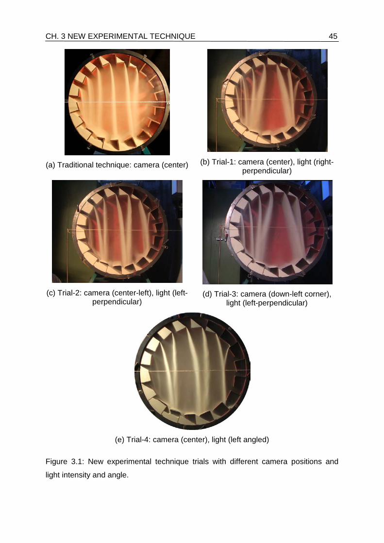
CH. 3 NEW EXPERIMENTAL TECHNIQUE 45
(a) Traditional technique: camera (center)
(b) Trial-1: camera (center), light (right-
perpendicular)
(c) Trial-2: camera (center-left), light (left -
perpendicular)
(d) Trial-3: camera (down-left corner),
light (left -perpendicular)
(e) Trial-4: camera (center), light (left angled)
Figure 3.1: New experimental technique trials with different camera positions and
light intensity and angle.

46 CH. 3 NEW EXPERIMENTAL TECHNIQUE
(a) New technique original photo
(b) Final black and white (BW) photo to
Matlab
Figure 3.2: Transformation of the new experimental technique photos in black and
white.
3.3 New experimental work and scaling up the drum size
In order to verify the use of the new experimental technique, it is planned in this
chapter to carry out more experiments using the new technique. Also the drum size
was enlarged to be double the drum used for the experiments in Ch. 2. In the present
chapter more experiments are to be carried out on a test rig similar to the one
described previously in Ch. 2 except for the drum size that will be 1.0 m diameter and
0.3 cm length where the length to the diameter ratio (L/D) kept constant at 0.3.
Number of flights are as before 12 and 18. For the flight length ratios, it is planned to
study more flight length ratios than before as to be; 0.0, 0.375, 0.75 and 1.0. But It is
found during conducting the experiments that, the flight length ratio of 0.0 could only
be used for over loading drums. As it is found that the amount of solid needed for the
design loading point when using flight length ratio of 0.0 is very less and
consequently very early final discharge angle (see Fig. 3.3 ), because there is no any
tangential length of the flight and this will be nonsense to be applied in industry. Thus
it is recommended when using flight length ratio of 0.0 the drum should be
overloaded. Another observation from the experimental work affected also the
selection of the studied flight length ratios, is that the flight length ratio of 1.0 cannot

CH. 3 NEW EXPERIMENTAL TECHNIQUE 47 be used with 18 flights drum. As the spaces between the flights are small and a kind
of throttling of the solid happened and a formation of a bed at the bottom of the drum
is observed which is inconsistent with the definition of the optimum loading, as shown
in Fig. 3.4. Thus the flight length ratios choosed to be 0.375, 0.75 and 1.0 (for 12
flights only). Two materials are to be examined quartz sand of 0.2 mm particle
diameter and glass beads of 0.7 mm (back to Table 2.2 for the material properties).
For the same range of rotational speeds of 1, 3 and 5 rpm. The new experimental
work drum specifications and operating parameters are listed in Table 3.1.
Figure 3.3: Flight length ratio of 0.0 shows very less amount of solid at design loading.
(a) 18 flights (formation of bed)
(b) 12 flights (no bed)
Figure 3.4: Problems when using flight length ratio 1.0 with the 18 flights.

48 CH. 3 NEW EXPERIMENTAL TECHNIQUE
Table 3.1: Specifications of the drum and operating parameters of the new experimental work
Drum diameter 1.0 m Drum length 0.3 m Flight length ratio 0.375, 0.75 and 1.0 (12 flights only) Number of flights 12 and 18 Rotational Speed 1, 3 and 5 rpm
The experimental procedure is the same as discussed in Ch. 2. The data will be
extracted based on the automated image analysis method except for the tip angles
and curtains falling height measurements, the manual method is used. Same data
fitting method for the experimental results used in Ch. 2 is used here in the current
work.
3.4 Results and discussions
The measured average FUF cross section area is plotted versus the drum filling
degree in the following Figures.
3.4.1 Influence of number of flights
Figure 3.5 shows the influence of the drum filling degree on the measured FUF
cross sectional area for rotational speeds of 1, 3 and 5 rpm and the number of flights
12 and 18 at the same flight length ratio of 0.75. From Fig. 3.5 (a) for quartz sand it
can be noted that the saturation (maximum) value of the measured FUF cross
sectional area are in the range of 105 cm2. For the 12 flights drum the increase in the
rotational speed from 1 to 5 rpm caused an increase in the required design loading
filling degree from 7.5 to 9.5%, respectively, which is an increase of 26.6%. For the
drum of 18 flights that increase is from 11 to 13.4 %, a 21.8 % increase in the design
loading filling degree. By comparing the values of the filling degree required for the
design loading points of the 12 flights drum to the 18 flights drum an average
increase of 44% can be observed.
Figure 3.5 (b) for glass beads show comparable values of the FUF cross
sectional area in the range of 126 cm2. For the 12 flights drum the required filling

CH. 3 NEW EXPERIMENTAL TECHNIQUE 49 degree for design loading increases from 7.3 to 9% when the rotational speed
increases from 1 to 5 rpm, respectively, by a percentage increase of 23. For the drum
with 18 flights the filling degree varied from 12.3 to 14%, respectively, which is 13.8%
increase. In order to achieve design loading conditions using 18 flights, in average 60
% more material should be added when compared with the amount of material used
by the 12 flights drum for the same design loading conditions.
Figure 3.5: Measured FUF cross sectional area versus drum filling degree for
various rotational speeds and number of flights (a) quartz sand (b) glass beads.
4 6 8 10 12 14 1620
40
60
80
100
120
140
HFU
F in
cm
2
quartz sanddp 0.2 mmΘA 32.4o
ρb 1570 kg/m3
nF 12 nF 181 rpm3 rpm5 rpm
(a)l2/l1 0.75
D 1.0 mL 0.3 m
2 4 6 8 10 12 14 16fd in %
20
40
60
80
100
120
140
HFU
F in
cm
2
nF 12 nF 181 rpm3 rpm5 rpm
(b)l2/l1 0.75
glass beadsdp 0.7 mmΘA 28.0o
ρb 1560 kg/m3
D 1.0 mL 0.3 m

50 CH. 3 NEW EXPERIMENTAL TECHNIQUE 3.4.2 Influence of flight length ratio
Figure 3.6 illustrates the variation of the measured FUF cross sectional area
versus the drum filling degree for various rotational speeds from 1 to 5 rpm and two
flight length ratios of 0.375 and 1.0 at the same number of flights of 12.
Figure 3.6 (a) for quartz sand with particle diameter of 0.2 mm showed an
increase in the average measured FUF cross sectional area from 70 to 120 cm2 on
average while changing the flight length ratio from 0.375 to 1.0 resulted in a
percentage increase of 71.4. At a flight length ratio of 0.375 the required drum filling
degree for the design point increased from 4.1 to 5.3% when the rpm changes from 1
to 5 which is an increase of 29%. For the flight length ratio of 1.0 an increase was
observed from 10 to 12.1%, which is a percentage increase of 21. Comparing the
results of the two flight length ratios it can be seen that the required drum filling
degree for the design loading increases by an average of 120%.
In Fig. 3.6 )b( for glass beads with particle diameter of 0.7 mm showed an
increase in the average measured FUF cross sectional area from 70 to 125 cm2 while
changing the flight length ratio from 0.375 to 1.0 which is a percentage increase of
78. At the flight length ratio of 0.375 the required drum filling degree for the design
loading point changed from 4.7 to 5.8% when the rpm changes from 1 to 5, which is
an increase of 23.4%. For the flight length ratio of 1.0 an increase was observed from
10 to 12%, which is a percentage increase of 20. Comparing the results of the two
flight length ratios it can be seen that the required drum filling degree for the design
loading condition increased on average by 120%.

CH. 3 NEW EXPERIMENTAL TECHNIQUE 51
Figure 3.6: Measured FUF cross sectional area versus drum filling degree for
various rotational speeds and flight length ratios at the same number of flights of 12
(a) quartz sand (b) glass beads.
3.4.3 Comparisons with models from literature
Table 3.2 lists all the experimental results performed on the large size drum of
1.0 m diameter including all of operating conditions. Also it shows the deviations from
the design loading models of Ajayi and Sheehan, 2012b (Eq. (1.4)) and the
developed model suggested by the current work (Eq. 2.1). The comparisons of the
deviations from the models revealed that the current work model was the better to
predict the design loading (±11%) than the one of Ajayi and Sheehan (±17%).
0 2 4 6 8 10 12 14 160
20
40
60
80
100
120
140
160
HFU
F in
cm
2
quartz sanddp 0.2 mmΘA 32.4o
ρb 1570 kg/m3
nF 121 rpm3 rpm5 rpm
(a)l2/l1 1.0
l2/l1 0.375
D 1.0 mL 0.3 m
0 2 4 6 8 10 12 14 16fd in %
0
20
40
60
80
100
120
140
160
HFU
F in
cm
2
nF 121 rpm3 rpm5 rpm
(b)l2/l1 1.0
glass beadsdp 0.7 mmΘA 28.0o
ρb 1560 kg/m3
l2/l1 0.375
D 1.0 mL 0.3 m

52 CH. 3 NEW EXPERIMENTAL TECHNIQUE
Table 3.2: Experimental results and deviation from models
No. Material
used
dp
(mm)
N
(rpm)
nF
--
l2/l1
--
HFUF
(cm2)
fdesign load
(%)
Deviation from models (%)
Ajayi 2012
Karali 2015
1 Glass Beads 0.7 1 12 0.375 71.15 ±0.4 4.5 34.7 18.8
2 Glass Beads 0.7 3 12 0.375 72.21 ±0.6 5.2 18.3 4.4
3 Glass Beads 0.7 5 12 0.375 72.13 ±0.4 5.7 7.8 -4.9
4 Glass Beads 0.7 1 12 0.75 111.6 ±0.5 7.4 28.5 13.4
5 Glass Beads 0.7 3 12 0.75 110.3 ±0.3 8.1 16.0 2.4
6 Glass Beads 0.7 5 12 0.75 112.2 ±0.5 8.9 7.4 -5.2
7 Glass Beads 0.7 1 12 1.0 130.2 ±0.6 10 11.0 -2.1
8 Glass Beads 0.7 3 12 1.0 131.6 ±0.7 11.3 -0.8 -12.5
9 Glass Beads 0.7 5 12 1.0 131.0 ±0.5 12.1 -7.7 -18.6
10 Glass Beads 0.7 1 18 0.375 77.38 ±0.6 6.2 6.3 -6.2
11 Glass Beads 0.7 3 18 0.375 77.26 ±0.6 6.9 -4.6 -15.8
12 Glass Beads 0.7 5 18 0.375 77.98 ±0.6 7.8 -14.8 -3.8
13 Glass Beads 0.7 1 18 0.75 95.69 ±0.5 11.6 -29.7 -20.6
14 Glass Beads 0.7 3 18 0.75 95.73 ±0.4 12.7 -35.8 -27.4
15 Glass Beads 0.7 5 18 0.75 96.94 ±0.8 13.7 -39.7 -31.9
16 Quartz Sand 0.2 1 12 0.375 71.27 ±0.7 4.1 48.1 30.7
17 Quartz Sand 0.2 3 12 0.375 71.03 ±0.5 4.8 26.1 11.2
18 Quartz Sand 0.2 5 12 0.375 70.63 ±0.6 5.3 13.5 0.2
19 Quartz Sand 0.2 1 12 0.75 102.5 ±0.5 7.6 15.0 1.4
20 Quartz Sand 0.2 3 12 0.75 100.6 ±0.5 8.5 0.9 -11.0
21 Quartz Sand 0.2 5 12 0.75 101.7 ±0.4 9.5 -8.8 -19.5
22 Quartz Sand 0.2 1 12 1.0 121.8 ±0.5 9.9 4.8 -7.5
23 Quartz Sand 0.2 3 12 1.0 122.4 ±0.4 11.1 -6.0 -17.1
24 Quartz Sand 0.2 5 12 1.0 122.8 ±0.4 12 -12.8 -23.1

CH. 3 NEW EXPERIMENTAL TECHNIQUE 53
Table 3.2-continoued: Experimental results and deviation from models
No. Material
used
dp
(mm)
N
(rpm)
nF
--
l2/l1
--
HFUF
(cm2)
fdesign load
(%)
Deviation from models (%)
Ajayi 2012
Karali 2015
25 Quartz Sand 0.2 1 18 0.375 65.54 ±0.5 6 -6.9 -17.9
26 Quartz Sand 0.2 3 18 0.375 66.9 ±0.5 7 -18.6 -28.2
27 Quartz Sand 0.2 5 18 0.375 65.6 ±0.5 8 -30.1 -21.0
28 Quartz Sand 0.2 1 18 0.75 104.6 ±0.6 11 -19.0 -8.4
29 Quartz Sand 0.2 3 18 0.75 103.7 ±0.4 12.4 -28.7 -19.5
30 Quartz Sand 0.2 5 18 0.75 104.2 ±0.3 13.5 -34.2 -25.7
3.4.4 Scaling up the drum size
As described before the current chapter presented more experiments using a
larger drum size as the scaling up process. Where the drum diameter increased from
0.5 m (old experiments in Ch. 2) to 1.0 m (new experiments). Figure 3.7 depicts the
scaling up results based on comparing the required design loading filing degree of
the new experiments to the old one at the same operating conditions. The
comparison reveals that in most cases of operating conditions, the required filling
degree for design loading of the higher drum diameter (D=1.0 m) is less than of the
(D=0.5 m). Except for the cases of lower flight length ratio, both filling degrees were
almost the same. The average of the deviation was about -9 % as shown with the
shaded area in Fig.3.7. It should be mentioned that however the comparisons show
decrease in the filling degree for the 1.0 m diameter drum rather than the 0.5 m
diameter drum, but sure the total holdup (kg of solid) needed is much higher and in
average was about 60%.

54 CH. 3 NEW EXPERIMENTAL TECHNIQUE
Figure 3.7: Comparison between the results of the experimental data from small drum (D=0.5 m) to (D=1.0 m) at the same operating conditions of design loading.
3.5 Correlation development
Based on all of the experimental data presented in Ch. 2 and Ch. 3 a correlation
has been developed using the power function regression analysis as given in Eq.
(3.1). Including all of the studied parameters, mostly in the form of dimensionless
groups to help for the scaling up of the data (Froude number (Fr) was chosen to
substitute the rpm). Table 4.2 lists all of the valid ranges of the correlation's
parameters. The deviation of the calculated results from the correlation to the actual
experimental results is shown in Fig. 3.8, where the shaded area represents the root
mean square deviation (RMSD) with a factor of 3.4.
( ) 353.08390
1
2941005200130351052.01tan9.4% 043.0 l
..
F..
b.
Aploaddesign llnFrρθdDf
−= (3.1)
By means of this correlation the point of under loading can be determined and
avoided by changing some design parameters to the drum such; as the number of
flights or the flight length ratio.
0 5 10 15 20fdesign for old expriments (D=0.5 m) in %
0
5
10
15
20
f desi
gn fo
r new
exp
rimen
ts (D
=1.0
m)
in %
-9 %

CH. 3 NEW EXPERIMENTAL TECHNIQUE 55
Table 3.2: Correlation valid ranges
Parameter Units Valid Range
Drum characteristics
Drum diameter D m 0.5 - 1.0 Drum length L m 0.15 - 0.3 Drum length to Diameter ratio
L/D – 0.3
Rotational speed N rpm 1 - 5 Froude Number Fr – 0.000279 - 0.013
Material properties
Particle diameter dp m 0.0002 - 0.002 Material dynamic angle of repose
θA o 25.7 - 62.3
Material consolidated bulk Density
ρb kg/m3 1550 - 4630
Flight characteristics (rectangular)
Total number of flights
nF – 12 - 18
Flight tangential to radial length ratio
l2/l1 – 0.375 - 1.0
Flight radial length l1 m 0.05 - 0.1
Figure 3.8: Deviation of correlation results from experimental results for the same
operating conditions.
0 5 10 15 20fdesign from experimental reults in %
0
5
10
15
20
f desi
gn c
alcu
late
d fro
m c
orre
latio
n in
%
±3.4 %

56 CH. 3 NEW EXPERIMENTAL TECHNIQUE

57
Chapter 4 Determination of the discharge characteristics 4.1 Overview
Previously In Ch. 2 and Ch. 3 a lot of experiments were performed to assess the
optimum loading of a flighted rotary drum. Furthermore studies for the discharge
characteristics of the solid which leaves the flights to the gas-borne area are needed.
As they determines the amount of solid will present in the gas-borne phase and its
disperse nature. Which influences the overall performance of the drum. The
discharge characteristics to be studied in the present chapter are: kinetic angle of
repose of the solid reside inside the flights, holdup of the solid carried by the flights,
final discharge angle, height and time of fall. These discharge characteristics are to
be determined as a continuous function of the flight angular position. Assuming a
uniform distribution over the drum length (axial direction as described previously in
Ch. 2).
The recorded videos of the design loading points from the experimental work
presented in Ch. 2 and Ch. 3 are to be analyzed. The analysis relies on playing the
recorded video then tracing one flight from the 9 o’clock position to the final discharge
position (emptying point). The video has to be stopped arbitrarily at many positions in
between to extract photos of interest. These photos are to be analyzed using a
typical manual image analysis method described previously in Ch. 2 through
measurement of solid areas of interest, angles and distances of fall. Some

58 CH. 4 DETERMINATION OF THE DISCHARGE CHARACTERISTICS geometrical parameters are needed in the present chapter and must first be defined
as follows.
4.2 Geometrical parameters
Figure 4.1 shows some geometrical parameters of the flighted rotary drum
needed for the present study: flight tip angle ( discharge angle (δ )), final discharge
angle ( Lδ ), dimensions of the flight; radial length ( 1l ) and tangential length ( 2l ) and
effective radial distance ( Hr ) of the flight given by
1lRrH −= (4.1)
where R is the drum radius, the characteristic angle of the flight made by the
tangential length (α ) given by
Hrlα 2tan = . (4.2)
4.3 Kinetic angle of repose of the solid residing inside the flight
The kinetic angle of repose generally can be defined as the angle of stability of a
granular (powder) material residing on a surface. For instance, if a granular material
is poured onto a flat surface, it will form a pile whose stability angle with the
horizontal plane is called the static angle of repose. This angle of repose is affected
by the solid cohesivity.
Particles within a flight in a rotary drum will also form an angle of repose with the
horizontal plane, which will depend on the angular position of the flight. Since the
angle of repose is affected by the drum rotational speed, it is called the dynamic
(kinetic) angle of repose (J. Mellmann, 2001 and X. Liu et al., 2005).

CH. 4 DETERMINATION OF THE DISCHARGE CHARACTERISTICS 59
(a) (b)
Figure 4.1: Geometrical parameters (a) schematic diagram (b) experimental photo.
In a flighted rotary drum the material residing in a flight is tilted due to the rotation
of the drum, and the avalanches will start when the tilting surface of the material
exceeds the maximum angle of stability (Bagnold, 1954 and Gray, 2001). At this
point, the material organizes itself to reach the angle of repose by cascading the
extra material like an avalanche and trying to achieve the stable position again.
Therefore, the avalanche formation depends on the frequency of material surface
reaching the upper angle of repose, rather than change in the flight position.
Increasing the frequency leads to the particles continuously rolling down over the
surface of the static material in the flight which depends on the drum speed. This will
continue until the flight is emptied of the material at a certain angle (final discharge
angle) less than 180o (Sunkara, 2013).
Various geometrical based models were developed to investigate the discharge
characteristics from a flighted rotating drum. All of these models depend on defining a
model to describe the variation of the kinetic angle of repose of the solid residing
inside the flight as a continuous function of the flight tip angle, where the kinetic angle
of repose was used to determine the surface of the solid in each flight, and therefore
the holdup can be estimated geometrically as the area surrounded by this surface
(Porter, 1963; Kelly and O’Donnel, 1968; Glikin, 1978; Baker, 1988; Kelly, 1992;

60 CH. 4 DETERMINATION OF THE DISCHARGE CHARACTERISTICS Sherritt et al., 1993; Wang et al., 1995; Van Puyvelde, 2009; Lee and Sheehan, 2010 and Sunkara et al., 2013b). It was stated by Glikin, 1978 and followed by
other researchers, that it is difficult to model the drum with a single relation for the
flight holdup during the period of discharge. Hence, the discharge period should
divided into regions based on the range values of the kinetic angle of repose and the
angular position.
Schofield and Glikin, 1962 (Eq. (4.3)) developed the first model to calculate the
kinetic angle of repose of the solid residing inside the flight. The conventional two
segment flight was used in the model by applying the force balance acting at the tip
of the flight and assuming the material surface is smooth and approximately a
straight line. The kinetic angle of repose from their model depends on the
circumferential position of the flight (δ ), the geometrical parameters (described
previously in 4.1), the Froude number (Fr) given by
gRωFr
2
= (4.3)
where ω is the drum angular velocity and μ is the dynamic friction coefficient.
δ)μδ()Rr(Frα
δ)μδ()Rr(Frαμ
γH
H
cossincos
sincoscostan
+−
−+= . (4.4)
The dynamic friction coefficient ( μ ) can be taken as tan( AΘ ), where AΘ is the solid
material property dynamic angle of repose (the angle of repose of the free bed
surface at the bottom of the drum, Sunkara, 2013). Whereas in the present study it is
estimated by iterative calculations using Eq. (3.4) based on known measured kinetic
angles of repose ( γ ) at different flight discharge angles ( δ ). Finally, the calculated
dynamic friction coefficient is used to calculate the Schofield and Glikin, 1962
kinetic angle of repose ( γ ) and compare it with the experimental results.
The measured kinetic angle of repose of the solid residing inside the flight versus
the angular position (flight discharge angle) is plotted in the following for different

CH. 4 DETERMINATION OF THE DISCHARGE CHARACTERISTICS 61
materials and operating parameters at design loading conditions. The data points in
all figures correspond to the experimental measurements and each point represents
one image that was extracted from the video at a specific flight angular position.
Figure 4.2 depicts the influence of the discharge angle on the measured kinetic
angle of repose for two rotational speeds (1 and 5 rpm) and two number of flights (12
and 18) at the same flight dimensions. The lines represent the fitting curves
(polynomial fitting). It is observed that the kinetic angle of repose increases in
average by 2-7o during the initial period of discharge and then decreases in the last
stage. This fact as discussed before is mainly attributed to the fluctuating avalanching
behavior of the solid residing inside the flight. Also it is clear from Fig. 4.2 that
changing the discharge angle has less influence on the kinetic angle of repose than
lowering the speed of rotation (rpm). As the rpm increases, a shifting of the peak
points is observed. It shown in Fig. 4.2 that increasing the number of flights from 12
to 18 at the same flight dimensions, increases the kinetic angle of repose. This can
be attributed to the increase in the holdup carried by the flights which will increase
the frequency of the avalanches relative to the smaller number of flights.
Figure 4.3 illustrates the influence of the discharge angle on the measured kinetic
angle of repose for two rotational speeds (1 and 5 rpm) and two flight length ratios
(0.75 and 0.375) for a constant number of flights. It can be seen that the change in
the flight dimensions has nearly no influence on the kinetic angle of repose when
compared to the speed of rotation.
In Figs. 4.2 and 4.3 it can be noted that the values of the kinetic angle of repose
which were calculated based on Schofield and Glikin, 1962 model (Eq. (4.4)) are
almost constant for each case without fluctuation compared to experimental results.
This fact is mainly attributed to the assumptions used in the model. Also it is worth
noting that, because their model does not include the effect of the number of flights,
the kinetic angles calculated based on their model and shown in Fig. 4.2 only
consider the influence of the speed of rotation.

62 CH. 4 DETERMINATION OF THE DISCHARGE CHARACTERISTICS
Figure 4.2: Variation of measured kinetic angle of repose of the solid reside inside a
single flight against the flight discharge angle for various rotational speeds and
number of flights at design loading conditions, (a) quartz sand (b) glass beads (c)
steel balls.
0 20 40 60 80 100 120 14020
25
30
35
40
45
Kine
tic a
ngle
of r
epos
e γ
in o
quartz sanddp 0.2 mmΘA 32.4o
ρb 1570 kg/m3l2/l1 0.75
nF 12nF 18
nF 12
nF 18(a)
rpm 1rpm 5
Schofield and Glikin
0 20 40 60 80 100 120 14020
25
30
35
40
45
Kine
tic a
ngle
of r
epos
e γ
in o
l2/l1 0.75nF 12nF 18
rpm 1rpm 5
nF 12
nF 18
glass beadsdp 0.7 mmΘA 28.0o
ρb 1560 kg/m3
(b)
Schofield and Glikin
0 20 40 60 80 100 120 140
Discharge angle δ in o
20
25
30
35
40
45
Kine
tic a
ngle
of r
epos
e γ
in o
l2/l1 0.75nF 12nF 18
nF 12
nF 18
steel ballsdp 0.8 mmΘA 28.5o
ρb 4630 kg/m3
(c)
rpm 1rpm 5
Schofield and Glikin
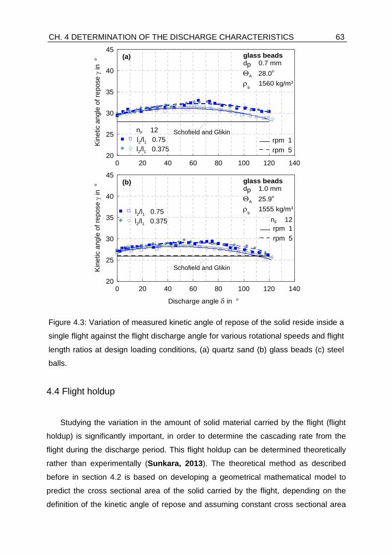
CH. 4 DETERMINATION OF THE DISCHARGE CHARACTERISTICS 63
Figure 4.3: Variation of measured kinetic angle of repose of the solid reside inside a
single flight against the flight discharge angle for various rotational speeds and flight
length ratios at design loading conditions , (a) quartz sand (b) glass beads (c) steel
balls.
4.4 Flight holdup
Studying the variation in the amount of solid material carried by the flight (flight
holdup) is significantly important, in order to determine the cascading rate from the
flight during the discharge period. This flight holdup can be determined theoretically
rather than experimentally (Sunkara, 2013). The theoretical method as described
before in section 4.2 is based on developing a geometrical mathematical model to
predict the cross sectional area of the solid carried by the flight, depending on the
definition of the kinetic angle of repose and assuming constant cross sectional area
0 20 40 60 80 100 120 14020
25
30
35
40
45
Kin
etic
ang
le o
f rep
ose γ
in o
l2/l1 0.75l2/l1 0.375
nF 12
glass beadsdp 0.7 mmΘA 28.0o
ρb 1560 kg/m3
rpm 1rpm 5
(a)
Schofield and Glikin
0 20 40 60 80 100 120 140
Discharge angle δ in o
20
25
30
35
40
45
Kin
etic
ang
le o
f rep
ose γ
in o
l2/l1 0.75l2/l1 0.375 nF 12
glass beadsdp 1.0 mmΘA 25.9o
ρb 1555 kg/m3
rpm 1rpm 5
(b)
Schofield and Glikin

64 CH. 4 DETERMINATION OF THE DISCHARGE CHARACTERISTICS along the drum. Experimentally there are mainly two methods: the first, by directly
weighing the amount of solid carried by the flight at different discharge positions; in
this method it is necessary to stop the drum at different arbitrary positions and collect
the solid from the specified flight to directly measure its weight; the second, by
tracking the boundary lines of the solid residing inside the flight to find the cross
sectional areas. This tracking requires extraction of multiple images at different
discharge positions from the recorded videos by stopping the footage at these
positions then analyzing the images to calculate the areas. Then the calculated areas
per unit drum length are converted to mass using the measured bulk density.
Although the first method is more reliable as it measures the mass of the solid more
precisely than the second method, this method requires suddenly interrupting the
drum to collect the solid and can cause a kind of non-uniform distribution of the solid.
In the present work, as described before, the calculation is experimentally determined
based on tracking the boundary lines of the solid using the image analysis methods
(described in Ch. 2). In the following, the measured flight holdup is plotted versus the
discharge angle.
Figure 4.4 represents the effect of varying the discharge angle of the individual
flight holdup for different rpm (1 to 5) and two numbers of flights (12 and 18) for
constant flight dimensions and design loading conditions. Figure 4.4 shows that at
any operating condition of the drum, the maximum holdup of the FUF is attained at 9
o’clock position (0o discharge angle) as the flight at that moment carries the largest
amount of solid. Then, due to the rotation of the drum, the angular position of that
flight (FUF) increases and the flight holdup decreases until the flight becomes empty.
This fact is supported by the change in the kinetic angle of repose described before
in Section 4.2. The final discharge angle can be estimated from the graphs as the
amount of holdup reaches zero. The measured flight holdup can be noticed to have a
curvilinear distribution, characterized by a dome its position varied according to the
operating condition, where the dashed line represents the uniform distribution
assumed by Glikin, 1978 for only one case where the final discharge angle takes
place at 180o. It can be seen from Fig. 4.4 that increasing the rpm or the number of
flights yields an increase in the average flight holdup due to the increase of total
holdup needed for the design loading.

CH. 4 DETERMINATION OF THE DISCHARGE CHARACTERISTICS 65
Figure 4.5 represents the effect of varying the discharge angle on the individual
flight holdup for different rpm (1 to 5) and two flight length ratios (0.75 and 0.375) for
a constant number of flights and design loading conditions. From Fig. 4.5 it can be
seen that changing the flight length ratio significantly affects the flight holdup, as
increasing the flight length ratio from 0.375 to 0.75 causes an increase in the flight
holdup by an average of 66%.
4.5 Final discharge angle of flight
The final discharge angle ( Lδ see Fig. 4.1 (a)) represents the position of the flight
at the end of the discharge period in the upper half of the drum. It can be determined
directly from the recorded videos by stopping each video at the moment when a
traced flight becomes totally empty and then extracting the image to measure the
angle manually. Figures 3.4 and 3.5 give information about the final discharge angles
for different solids and operating conditions of the drum. As the final discharge angles
can be determined from Figs. 4.4 and 4.5 at the positions of zero flight holdup. The
measured final discharge angles are plotted versus the change in the rpm in the
following graphs.
Figure 4.6 (a) represents the variation of the final discharge angle with the
change in the rpm for different solids and two numbers of flights (12 and 18) for a
constant flight length ratio (0.75). It is shown from Fig. 4.6 (a) that the final discharge
angle increases as the rpm increases, this related to the increase of the flight holdup
which delays the emptying point at design loading conditions. Also it can be seen that
the final discharge angle is decreased as the number of flights is increased.
Figure 4.6 (b) shows the variation of the final discharge angle with the change in the
rpm for different solids and flight length ratios (0.375 and 0.75) for a constant number
of flights (12). It is shown from Fig. 4.6 (b) that the final discharge angle increases as
both the rpm and flight length ratio increases. When increasing the flight length ratio,
the flight dimensions become bigger and carry more solid, which delays the empting
point at design loading conditions.

66 CH. 4 DETERMINATION OF THE DISCHARGE CHARACTERISTICS
Figure 4.4: Influence of the flight discharge angle on the measured holdup of a
single flight for various rotational speeds and number of flights at design loading
conditions, (a) quartz sand (b) glass beads (c) steel balls.
0 20 40 60 80 100 120 140 160 1800
5
10
15
20
25
30
HF i
n c
m2
quartz sanddp 0.2 mmΘA 32.4o
ρb 1570 kg/m3
nF 12nF 18
1 rpm3 rpm5 rpm
(a)
l2/l1 0.75
Uniform distribution (Glikin, 1978)
0 20 40 60 80 100 120 140 160 1800
5
10
15
20
25
30
HF i
n c
m2
nF 12nF 18
1 rpm3 rpm5 rpm
(b)
l2/l1 0.75
glass beadsdp 0.7 mmΘA 28.0o
ρb 1560 kg/m3
0 20 40 60 80 100 120 140 160 180
Discharge angle δ in o
0
5
10
15
20
25
30
HF i
n c
m2
nF 12nF 18
1 rpm3 rpm5 rpm
(c)
l2/l1 0.75
steel ballsdp 0.8 mmΘA 28.5o
ρb 4630 kg/m3

CH. 4 DETERMINATION OF THE DISCHARGE CHARACTERISTICS 67
Figure 4.5: influence of the flight discharge angle on the measured holdup of a
single flight for various rotational speeds and flight length ratios at design loading
conditions (a) quartz sand (b) glass beads (c) steel balls.
0 20 40 60 80 100 120 140 160 1800
5
10
15
20
25
30
HF i
n c
m2
nF 121 rpm3 rpm5 rpm
(a)
l2/l1 0.75l2/l1 0.375
glass beadsdp 0.7 mmΘA 28.0o
ρb 1560 kg/m3
0 20 40 60 80 100 120 140 160 180
Discharge angle δ in o
0
5
10
15
20
25
30
HF i
n c
m2
nF 121 rpm3 rpm5 rpm
(b)
l2/l1 0.75l2/l1 0.375
glass beadsdp 1.0 mmΘA 25.9o
ρb 1555 kg/m3

68 CH. 4 DETERMINATION OF THE DISCHARGE CHARACTERISTICS
Figure 4.6: Variation of final discharge angle versus drum rpm for different materials
and different operating conditions (a) different number of flights and same flight
length ratio (b) different flight length ratios and same number of flights. At design
loading conditions.
4.6 Flight cascading rate
The cascading rate from a flight can be represented as a dimensionless quantity
by the changes of the flight filling degree ( )(δFf ) with the discharge angle (δ ) as
noted in Eq. (4.6). Where the flight filling degree ( )(δFf ) is the flight holdup per unit
length ( )(δFH ) divided by the total drum volume per unit length ( drumV ) (Eq. (4.5)), bρ
is the solid bulk density, ω is the drum angular velocity, and R and L are the drum
1 2 3 4 580
100
120
140
160
Fina
l dis
char
ge a
ngle
δL i
n o
nF 12nF 18
quartz sand 0.2 mmglass beads 0.7 mmsteel balls 0.8 mm
l2/l1 0.75
Fr = 0.000280.0025 0.007
(a)
1 2 3 4 5
rpm
80
100
120
140
160
Fina
l dis
char
ge a
ngle
δL i
n o
nF 12
l2/l1 0.375glass beads 0.7 mmglass beads 1.0 mm
l2/l1 0.75
Fr = 0.00028 0.0025 0.007(b)

CH. 4 DETERMINATION OF THE DISCHARGE CHARACTERISTICS 69
radius and length, respectively. The flight cascading rate ( )(δFm ) with units of kg/s can
be drawn using Eqs. (3.5-3.6).
drum
FF V
Hf )(
)(δ
δ = (4.5)
LRm
dfd
b
FF2
)()(
πωρδδδ
=
−
(4.6)
The calculated flight cascading rates over the periods of discharge are found to
be with fluctuations, the fittings of the fluctuating curves are plotted against the
discharge angle in Fig. 4.7. Figure 4.7 (a) shows the influence of the discharge angle
on the flight cascading rate for quartz sand at two number of flights (12 and 18) and
constant flight length ratio (0.75) and rpm (3). It can be seen from Fig. 4.7 (a) that the
cascading rate is relatively high at the initial point of discharge as the flight has just
left the large amount of solid bulk. Then the cascading rate decreases until it attains a
minimum due to the decrease in the avalanching rate as the solid material returns
again to stability. After that, as the flight elevates to higher positions, the cascading
rate increases and attains a maximum at a certain point. Later the cascading rate
sharply decreases until the emptying point. It could be noticed that the initial
cascading rate for the case of drum with 18 flights is lower than the one of 12 flights.
On the contrary the maximum peak of the cascading rate of 18 flights is higher than
the one of 12 flights.
Figure 4.7 (b) depicts the influence of the discharge angle on the flight cascading
rate for glass beads at two flight length ratios (0.375 and 0.75) at constant rpm (3) andnumber of flights (12). It can be seen from Fig. 4.7 (b) that the initial cascading
rate for the lower flight length ratio (0.375) is higher than for the larger flight length
ratio (0.75). Later it is noticed that the cascading rate is much higher for the larger
flight length ratio (0.75) than the lower one (0.375). Overall, it could be concluded that
increasing the flight dimension causes the cascading rate to increase.

70 CH. 4 DETERMINATION OF THE DISCHARGE CHARACTERISTICS
Figure 4.7: Variation of the flight cascading rate with the discharge angle at design
loading conditions, (a) quartz sand at two number of flights and constant rpm and
flight length ratio (b) glass beads at two flight length ratios and same number of
flight and rpm.
4.7 Curtains height of fall
4.7.1 Measured height of fall
The cascading of the solid from the flights forms the same number of curtains as
there are active flights. The height of a curtain can be measured directly from the
photos as the vertical distance of a particle from the edge of the flight to the impact
point at the bottom of the drum. This height of fall determines the amount of time the
0 20 40 60 80 100 120 140 160 1800
0.0002
0.0004
0.0006
0.0008
Flig
ht c
asca
ding
rate
in k
g/s quartz sand 0.2 mm
nF 12nF 18
l2/l1 0.75rpm 3
fd = 9.4 %
fd = 13.7 %
0 20 40 60 80 100 120 140 160 180
Discharge angle δ in o
0
0.0002
0.0004
0.0006
0.0008
Flig
ht c
asca
ding
rate
in k
g/s glass beads 0.7 mm
l2/l1 0.75l2/l1 0.375
nF 12rpm 3
fd = 9 %
fd = 5 %

CH. 4 DETERMINATION OF THE DISCHARGE CHARACTERISTICS 71
particles reside in the gas-borne phase where they are exposed to the gas stream. The impact point differs according to the filling degree of the drum. For example, for
an overloaded drum most of the impact points from falling are at the solid bed in the
bottom of the drum, while for the case of design loaded drum the bottom solid bed no
longer exists (see Fig. 4.1). However in some cases the impact point is located at the
metal back side of an opposite flight. As a conclusion maximum falling height can be
achieved when operated the drum at the design loading filling degree with varied
locations of the impact points depend on the position of the flight (δ ).
Figure 4.8: Variation of the measured curtains falling height against the discharge
angle at design loading conditions, (a) quartz sand at two number of flights and
constant rpm and flight length ratio (b) glass beads at two flight length ratios and
same number of flights and rpm.
0 20 40 60 80 100 120 140 160 1800
0.2
0.4
0.6
0.8
1
h fal
l / D
l2/l1 0.75rpm 3
nF 12nF 18
quartz sand 0.2 mm
fd = 9.4 %
13.7 %
0 20 40 60 80 100 120 140 160 180
Discharge angle δ in o
0
0.2
0.4
0.6
0.8
1
h fal
l / D
nF 12rpm 3l2/l1 0.75 l2/l1 0.375
glass beads 1.0 mm
fd = 9 %
5 %

72 CH. 4 DETERMINATION OF THE DISCHARGE CHARACTERISTICS 4.7.2 Mean height of fall
From literature, Blumberg and Schlünder, 1996, proposed a semi empirical
relation (Eq. (4.7)) to estimate the mean height of fall ( fallh ) as a function of the drum
filling degree (f), the solid material dynamic angle of repose ( AΘ ) and the flight length
ratio (l2/l1).
( ) ( )130
1
2211850.
AfallllΘfR.h
+−= (4.7)
However, the valid range of the filling degree was observed to be too high for
industrial applications. 4.02.0 ≤≤ f , 8.04.0 ≤Θ≤ A and 0.1/75.0 12 ≤≤ ll .
In order to calculate and compare the measured mean height of fall of the current
experimental results with correlations from literature, the following relation could be
used.
( ) δδδ
δ
dhhL
fallL
fall ∫=0
1 (4.8)
Table 4.1 outlines the comparison of the measured mean height of fall of the
current experimental work with the one calculated using the correlation of Blumberg and Schlünder, 1996. It is shown that the correlation of Blumberg and Schlünder, 1996 failed in the prediction of the measured height of fall with high deviation
specially for the lower filling degree conditions. This is mainly due to that the
correlation is valid for over-loaded drums.
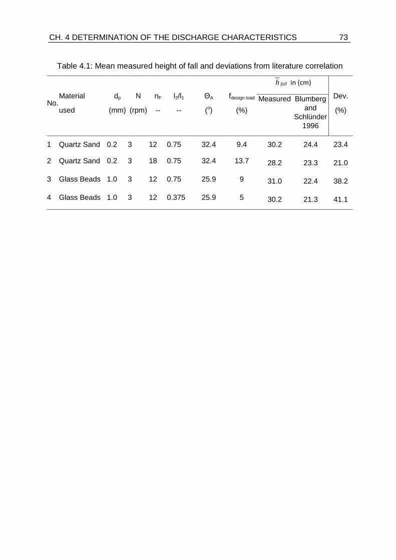
CH. 4 DETERMINATION OF THE DISCHARGE CHARACTERISTICS 73
Table 4.1: Mean measured height of fall and deviations from literature correlation
No. Material
used
dp
(mm)
N
(rpm)
nF
--
l2/l1
--
ΘA
(o)
fdesign load
(%)
fallh in (cm)
Dev.
(%) Measured Blumberg
and Schlünder
1996
1 Quartz Sand 0.2 3 12 0.75 32.4 9.4 30.2 24.4 23.4
2 Quartz Sand 0.2 3 18 0.75 32.4 13.7 28.2 23.3 21.0
3 Glass Beads 1.0 3 12 0.75 25.9 9 31.0 22.4 38.2
4 Glass Beads 1.0 3 12 0.375 25.9 5 30.2 21.3 41.1

74 CH. 4 DETERMINATION OF THE DISCHARGE CHARACTERISTICS

75
Chapter 5 Axial transport
5.1 Introduction
The study of the axial transport of the solid through a flighted rotary drum aims to
follow the motion behavior of the solid along the drum length under the effect of
operating conditions. The axial transportation of the solid through a flighted rotating
drum is influenced by: the drum slope to the horizontal, the drum rotational speed,
the lifting of the solid by the flights, the disperse nature into the gas stream, the
bouncing in the gas and rolling and the sliding of the particles on impact with the
bottom of the dryer (Britton et al., 2006 and Rojas et al., 2010). Hence the studying
of the axial transport is much complicated and a lot of assumptions for simplifications
are needed (Duchesne et al., 1996 and Renaud et al., 2000). The main output
results from studying the axial transport phenomena are: the estimation of the mean
retention time (residence time) elapsed by the solid in the drum starting from the feed
end to the discharge end and the solid mass feed rate.
The determination of the optimum residence time needed for the solid in a rotary
drum (for example rotary dryer) is of importance which determines the quality of the
product. Smaller residence time causes uneven drying of the feedstock, whereas the
higher residence times lead to over drying of the material which involves unaccepted
changes in the product shape and properties and moreover huge energy loss
(Friedman and Marshall, 1949; Tarhan et al., 2010 and Sunkara, 2013).

76 CH. 5 AXIAL TRANSPORT 5.2 Physical description of the axial transport in a flighted rotary drum
Figure 5.1 gives information about the motion behavior of the solid in a flighted
rotating drum. Considering a single particle of the solid transported through the drum,
the particle is lifted up by the flight because of the rotation of the drum (from point A
to B see Fig. 5.1 (a) and (b)) and then it is falling down (from B to C). After the
particle leaving the flight it is travelling through the gas stream and subjected to drag
force in a direction parallel to the axis of the drum and a drag force opposing the
falling direction of the particle (see Fig. 5.1 (c)). The effect of the later is negligible
compared to the accelerating force due to gravity. At the impact point at the bottom of
the drum the particle can be rolling and sliding until it begin anther cascade cycle
(Glikin, 1978 and Cronin et al., 2011).
Because of the slope of the drum ( β ) a successful axial advance (X) by the
particle is observed during the fall. And the particle motion is forming a number of
cascade cycles with an axial advance till it discharges from the drum. The number of
cascades and the axial advance per cascade are determining the mean residence
time of the solid inside the drum. To determine the axial advance ( X ) by the particle,
the equation of motion should be applied as will be described in this chapter.
5.3 Models from literature
Many solid transport models of flighted rotary dryers have involved the
development of empirical relationships for the mean residence time (τ) from pilot-
scale experiments. While simplistic in nature, pilot-scale empirical relationships
generally lead to under prediction of measured values of the mean residence time in
industrial rotary dryers (Cao and Langrish, 1999). An alternative technique was
employed by researchers to determine the mean residence time using geometric
models arguments based on the holdup of flights over the discharge angle (Britton
and Sheehan, 2006). The mean residence time of solid in a rotary drum is influenced
by four components of particle movement along the drum: a) gravitational due to the
slope of the drum, b) drag of the gas on the particles for counter-current flow (this is
negative) c) bouncing of the particles on impact with the bottom of the dryer

CH. 5 AXIAL TRANSPORT 77
(a)
(b)
(c)
Figure 5.1: Falling of a particle in a flighted rotary drum inclined to the horizontal, (a)
cross sectional view (b) axial view (c) free body diagram showing external forces.

78 CH. 5 AXIAL TRANSPORT and d) rolling of the particles in the bed at the bottom of the dryer, specially for
overloaded dryers. The last two components are almost impossible to predict
theoretically and are therefore evaluated experimentally for each type of material
(Kemp and Oakley, 1997). Numerous equations have been proposed for the
estimation of the mean residence time in rotary drums, in the following are some
models from literature (Austin et al., 1978; Alvarez and Shene, 1994; Lisboa et al.,
2007; Thibault et al., 2010 and Sunkara, 2013) .
In many of these studies, only average holdups and solid feed rate were
considered (Kelly and O´Donnell, 1977). The mean residence time for the particles (
τ ) in these cases is given by
s
Tot
mH
=τ (5.1)
where TotH is the total drum holdup in kg, usually determined by suddenly stopping
the drum and subsequently weighing its contents and sm is the solid feed rate in kg/s.
One of the most frequently used empirical equation for residence time estimation
was proposed by Friedman and Marshall, 1949:
( ) sp
a
mdmL
DNL
59.0tan
8.139.0 ±=
βτ . (5.2)
Here the upper plus sign refers to the counter-current flow and the lower mince sign
refers to the co-current flow. β is the drum slope angle in degree, N is the rpm, L is
the drum length in m, D is the drum diameter in m and dp is the particle diameter in m
and am and sm are in kg/s.
Saeman and Mitchell, 1954 were the first to break away from the empirical
approach to calculating rotary dryer holdups adopted by previous researchers. They
analyzed material transport through the dryer in terms of incremental transport rates

CH. 5 AXIAL TRANSPORT 79 associated with individual cascade paths to yield a transport-rate distribution function.
By assuming a linear relationship between the horizontal displacement of the
particles due to the air flow and its velocity, they derived the following equation for the
mean residence time:
( ) ( )( )gumNDHfL
′±=
βτ
tan. (5.3)
Where ( )Hf is a cascade factor with values typically between 2 and π that increase
as solids holdup increases, and m′ is an empirical parameter (dimensional) for a
given material. The positive sign in Equation indicates the con-current flow and the
negative sign indicates the counter-current flow.
Schofield and Glikin,1962 derived the following residence time equation by
considering the drag exerted by the air flowing counter-currently to the particles:
( )
+
−
=Ng
y
guky
L avgavg
ravg
πδ
βτ
5.0
2
2
sin
(5.4)
where avgy is the average falling height, ru is the relative velocity between solid and
gas, avgδ is the average discharge angle corresponding to avgy and k is a factor for
the drag force (will be described in details later in Sec. 5.3).
In other publications the total residence time was calculated as the total number
of cascades of a particle moving along the drum times the sum of the time of lifting
and the time of falling per one cascade. Where the number of cascades can be
estimated based on the calculated axial advance of the particle per cascade. For
such reason a mathematical model was proposed by Kamke and Wilson, 1986. The
axial advance of the particle ( X ) per cascade was given by the following expression
( )( )( )( )
+−+= −
−
11
1
11
/tancos/tancos
ln1autKa
auk
tuXgfall
gfallg (5.5)

80 CH. 5 AXIAL TRANSPORT where 1a and k are constants depending on the drum inclination and drag coefficient
respectively, gu is the gas velocity, fallt is the falling time. The model has been
validated with an experimental drum of 1.2 m in diameter and 5.5 m in length, with six
centered flights and 12 flights installed to the outer shell of the dryer. The
experiments were performed with wood particles having a sphericity of 0.75 and
exposed to hot gas stream in con-current passion. The residence time was measured
by injecting a radioactive tracer particles at the inlet along with the feed. They noticed
that within a curtain, the particles may be effected by the other particles and shielding
of the gas flow can also occur. Due to this the model over predicted the data
collected, since the model assumes that the particles are independent to the gas
flow. They noted that the particles may be attributed as a bulk material and the mean
diameter can be used in order to measure the drag coefficient. It has been found that
the root mean square error was 109.6% in the case of discrete particle size whereas,
in case of mean diameter it was around 14.2%.
Recently, based on the analysis of a large amount of data found in the literature
on the operation of rotary drums of many applications, both on a pilot and an
industrial scale, Perry and Green,1999 proposed the following general correlation for
calculation of the mean residence time:
( ) DNLK
9.0tan βτ = (5.6)
where K is a parameter that depends on the number and format of the flights.
In the present chapter, a mathematical model is developed for the axial transport
based on applying the force balance on a falling particle from a flight in a rotary drum
using the available experimental measurements of the holdups and height of fall over
the discharge angle (described in Ch. 4).

CH. 5 AXIAL TRANSPORT 81 5.3 Current work model description
5.3.1 Model assumptions
• Uniform discharge characteristics along the drum (discussed in Ch.3)
• Each particle spent the same amount of time over the drum
• The particle is of a spherical shape and it remains its dimensions and shape
unchanged along the drum
• Neglect the rotational effect on the particle after leaving the flight
• Free and vertical fall of the particle (initially at zero velocity)
• Neglect the vertical drag force
• No slip condition of the gas on the particle surface
• Neglect transitional effects between the particle and the fluid
• Neglect the interactions between particles (free flowing - non cohesive)
5.3.2 Equationing
The free body diagram of the forces acting on a single particle falling freely from
a flight of a rotary drum at a certain discharge angle (δ ) and subjected to a gas flow
(assumed air) is shown in Fig. 5.1 (c). Applying the equation of motion on the particle
in the axial direction after considering the model assumptions (Maxey and Riley, 1983), reveals that;
∑= Forcesam x (5.7)
( ) 2sin rx ukmmg
dtdum β=
(5.8)
( ) 2sin rx ukg
dtdu
β=
(5.9)
where the upper minus sign refers to air following counter-current flows and the lower
positive is for co-current. β is the drum inclination angle, ru is the relative velocity
between the particle and the air as

82 CH. 5 AXIAL TRANSPORT
xar uuu ±= (5.10)
au is the air velocity and xu is the particle falling velocity component in x-direction.
The upper positive sign refers to counter-current flows and the lower mince sign is for
the con-current.
xu can be obtained by applying the free fall equation on the particle assuming the fall
from rest and then by resolving the falling velocity yu .
yg
uy =2
2
(5.11)
( ) ( )βsin221 ygyux =
(5.12)
The calculated xu is a function of the falling distance (y) which is already varying with
the flight position (δ ).
In order to simplify the solution, an average value of the falling distance can be
considered and calculated by the integration of the measured falling height over the
flight discharge angle (see Ch.4 Eq. (4.8)) as
( ) δδδ
δ
dhhyL
fallL
fallavg ∫==0
1 (5.13)
where Lδ is the measured final discharge angle at a specific operating conditions (see
Ch. 4)
( )βsin221
, avgavgx ygu = (5.14)
Then the average relative velocity can be calculated for known air velocity as
( )βsin221
, avgaavgr yguu ±= (5.15)

CH. 5 AXIAL TRANSPORT 83
Back to Eq. (5.8), the term k (presented before in Eq. (5.4)) can be calculated based
on the drag coefficient DC . The drag coefficient was evaluated using the commonly
used Schiller Naumann drag correlation (Glikin, 1978, Kamke and Wilson, 1986
and Karimi et al., 2012) as stated in the following;
p
a
p
D
dCk
ρρ5.1= (5.16)
2.0ReRe12
≤=DC
(5.17)
( ) 1000Re2.0
ReRe15.0112 687.0
≤<+
=DC
(5.18)
1000Re44.0 >=DC
(5.19)
a
pavgra duµ
ρ ,Re=
(5.20)
where pd is the particle diameter, pρ is the particle density, aρ is the fluid density, aµ
is the fluid dynamic viscosity and Re is a modified Reynolds number calculated based
on the relative velocity between the fluid and the particle.
The final solution of Eq. (5.3) gives the axial advance of the particle per one cascade
(lifting then falling) and it is found to be
( )( ) ( ) ( ) ( )2
,2,
2, 2
1sin21
avghfallavgravghfallavg tuktgX β= (5.21)
where ( )avghfallt , is the average falling time calculated based on the calculated average
falling height as
( ) ght fall
avghfall2
, = (5.22)

84 CH. 5 AXIAL TRANSPORT Then the number of cascades can be drawn by dividing the total drum length by the
axial advance per one cascade
XLC = (5-23)
During one cascade, the lifting time can be approximated as
Nt avgavg
avglift πδ
ωδ
==2
, (5.24)
where avgδ is the discharge angle (in radians) corresponding to the calculated
average height of fall, ω is the angular velocity in rad/s and N is the rotational speed
in rps
( )fallavg hδδ = . (5.25)
Thus the total average time elapsed by the particle in the drum (mean residence time
τ in sec) can be estimated from the following relation
( )( )avghfallavglift ttC ,, +=τ (5.26)
where ( )avghfallavglift tt ,, + is the total time per one cascade.
In order to calculate the total solid mass flow rate passing through the drum a new
average solid velocity should be introduced where the subscript (s) denotes the solid
material as
τLu savg =, (5.27)
The total drum holdup TotH (in m3/m) can be estimated using one of two methods: the
first is a direct way by using the proposed model that previously described in Ch. 2
(Eq. (2.1)) by the substitution of the measured flights holdups; the second is an
indirect way depending on the measured design loading filling degree by using the
following relation,
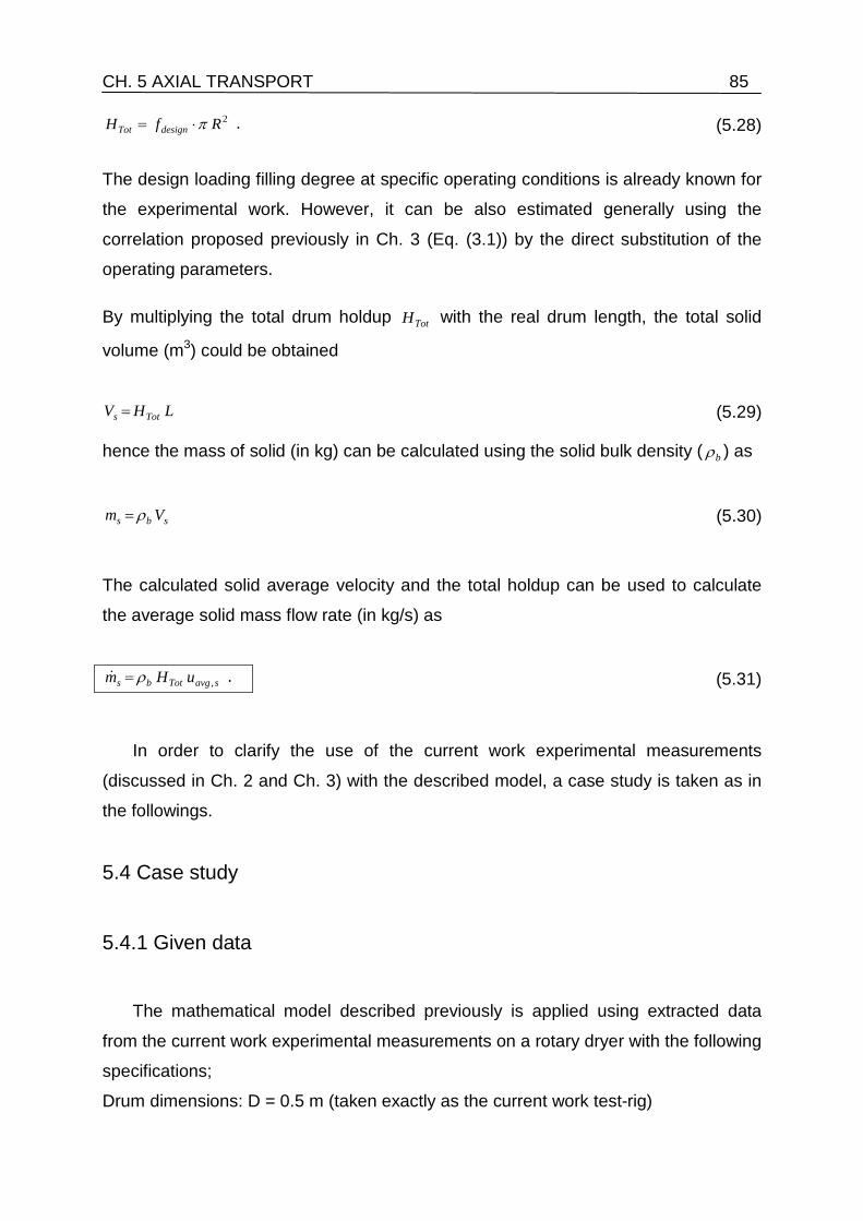
CH. 5 AXIAL TRANSPORT 85
2RfH designTot π⋅= . (5.28)
The design loading filling degree at specific operating conditions is already known for
the experimental work. However, it can be also estimated generally using the
correlation proposed previously in Ch. 3 (Eq. (3.1)) by the direct substitution of the
operating parameters.
By multiplying the total drum holdup TotH with the real drum length, the total solid
volume (m3) could be obtained
LHV Tots = (5.29)
hence the mass of solid (in kg) can be calculated using the solid bulk density ( bρ ) as
sbs Vm ρ= (5.30)
The calculated solid average velocity and the total holdup can be used to calculate
the average solid mass flow rate (in kg/s) as
savgTotbs uHm ,ρ= . (5.31)
In order to clarify the use of the current work experimental measurements
(discussed in Ch. 2 and Ch. 3) with the described model, a case study is taken as in
the followings.
5.4 Case study
5.4.1 Given data
The mathematical model described previously is applied using extracted data
from the current work experimental measurements on a rotary dryer with the following
specifications;
Drum dimensions: D = 0.5 m (taken exactly as the current work test-rig)

86 CH. 5 AXIAL TRANSPORT L = 2.5 m
N = 3 rpm (0.05 rps), ω = 0.314 rad/s
nF = 12, l2/l1 = 0.75
Drum slope ( β ) = 4o (0.0697 rad)
Solid properties: glass beads
dp = 1.0 mm
pρ = 2650 kg/m3
bρ = 1555 kg/m3
Fluid properties: Air at 115oC (400 K) (Cengle, 2003 and Incropera and DeWitt, 2006)
aρ = 0.8711 kg/m3
aµ = 0.000023 Pa.s
au = varied from 0.2 to 0.5 m/s.
Required: calculate for both cases of fluid flows, counter-current and con-current and
for the mentioned range of air velocity the followings; average axial advance per
cascade, mean residence time of the solid in the drum and average solid mass flow
rate at the design loading conditions. Using the current work experimental
measurements mentioned in Ch. 2 and Ch. 3.
5.4.2 Results
The mathematical model is applied and the variation of the results with the air
velocity for two types of flows; counter-current and con-current are illustrated in the
following figures.
Figure 5.2 represents the variation of the axial advance per one cascade of falling
particle with the air velocity for two types of flows counter-current and con-current. It
is obviously shown from Fig. 5.2 that the average axial advance of the case of
counter -current flow type is lower than the one of the con-current flow type. This is
mainly attributed to the higher drag coefficient ( k ) achieved by the counter-current

CH. 5 AXIAL TRANSPORT 87 flow. From Fig. 5.2 it can be seen that increasing the air flow rate causes a decrease
in the axial advance for the case of counter-current flow type where the air is resisting
the particle advance. While for the case of con-current flow type the axial advance
increases as the air flow rate increases.
Figure 5.2: Variation of the axial advance per one cascade of falling particle with the
air velocity for two types of flows counter-current and con-current.
Figure 5.3 depicts the variation of the mean residence time against the air
velocity for two types of flows counter-current and con-current. It is obviously shown
from Fig. 5.3 that the mean residence time elapsed by the solid in the drum of the
case of counter -current flow type is higher than the one of the con-current flow type.
This is related to the higher drag coefficient characterized the by the counter-current
flow. From Fig. 5.3 it can be seen that increasing the air flow velocity causes the
mean residence time to increase for the case of counter-current flow type as the drag
force increased. While for the case of con-current flow type the mean residence time
decreases as the air flow velocity increases as the drag force decreases.
Figure 5.4 illustrates the variation of the solid flow rate with the air velocity for two
types of flows counter-current and con-current. It is obviously shown from Fig. 5.4
that the average solid flow rate of the case of counter -current flow type is lower than
the one of the con-current flow type. This is mainly because of the higher residence
time and the hence the lower solid average velocity of the case of the counter-current
0.1 0.2 0.3 0.4 0.5 0.6Air velocity ua in m/s
0
0.5
1
1.5
2
2.5
3
3.5
4
Axia
l adv
ance
per
cas
cade
Xav
g in
cm
D 0.5 mL 2.5 mnF 12rpm 3fdesign 9%
Counter-Current Con-Current
glass beads 1.0 mm

88 CH. 5 AXIAL TRANSPORT flow. Figure 5.4 shows that increasing the air flow rate causes a decrease in the solid
flow rate for the case of counter-current flow type. While for the case of con-current
flow type the solid flow rate increases as the air flow rate increases.
Figure 5.3: Variation of the mean residence time with the air velocity for two types of
flows counter-current and con-current.
Figure 5.4: Variation of the solid mass flow rate with the air velocity for two types of
flows counter-current and con-current.
0.1 0.2 0.3 0.4 0.5 0.6Air velocity ua in m/s
56789
101112131415
Mea
n re
side
nce
time τ
in m
in
Counter-Current Con-Current
glass beads 1.0 mmD 0.5 mL 2.5 mnF 12rpm 3fdesign 9%
0.1 0.2 0.3 0.4 0.5 0.6Air velocity ua in m/s
0.2
0.3
0.4
0.5
0.6
0.7
0.8
Solid
mas
s flo
w ra
te in
ton/
hr Counter-Current Con-Current
glass beads 1.0 mmD 0.5 mL 2.5 mnF 12rpm 3fdesign 9%

CH. 5 AXIAL TRANSPORT 89
In order to validate the calculated mean residence time, the results is compared
with the commonly used correlations from literature; correlation of Friedman and Marshall, 1949 and later modified by Foust et al., 1960 described previously by Eq.
(5.2). The comparison is shown in Table 5.1 and reveals that the correlation of
Friedman and Marshall, 1949 failed in the prediction of the current work mean
residence time. As presented by the high deviations also shown in Table 5.1, same
conclusion found by many previous studies (Iguaz et al. 2003 and Abbasfard et al., 2013). Hence it is of importance to carry out experiments to determine the time taken
by the solid through the drum.
Table 5.1: Comparison of residence time with correlation from literature
va in
m/s
τ in min
Counter-current flow Con-current flow
Karali, 2015 Eq.
(5.26)
Friemann and
Marshall, 1949
deviation %
Karali, 2015 Eq.
(5.26)
Friemann and
Marshall, 1949
deviation %
0.20 10.94 6.38 -41.67 8.46 5.85 -30.84
0.25 11.36 6.46 -43.11 8.23 5.77 -29.83
0.30 11.81 6.55 -44.55 8.01 5.69 -28.96
0.35 12.29 6.64 -45.99 7.80 5.60 -28.24
0.40 12.82 6.74 -47.43 7.60 5.50 -27.68
0.45 13.39 6.85 -48.88 7.41 5.39 -27.30
0.50 14.02 6.96 -50.32 7.23 5.27 -27.15
Fitting of the current work results of the mean residence time using the model of
Perry and Green,1999 (Eq. (5.6)) reveals the fitting factor (K) equals to 22.7 in
average (see Eq. (5.32)).
( ) DNL
9.0tan7.22
βτ = (5.32)

90 CH. 5 AXIAL TRANSPORT 5.5 Direct application of the model (using in industry)
The described model for the axial transport can be a useful tool to be used in
industry to help for the design of rotary drums operated at optimum loading. The
model can estimate the total holdup needed for the drum to be operated at optimum
loading and also the mean residence time will elapsed by the solid as follows;
Design loading filling degree in %
( ) 353.08390
1
2941005200130351052.01tan9.4% 043.0 l
..
F..
b.
Aploaddesign llnFrρθdDf
−=
(5.33)
Total holdup of the drum at design loading in m2
( )
÷
= − 1001
353.08390
1
2941005200130351052.02 tan9.4 043.0 lRH.
.F
..b
.ApTot l
lnFrρθdDπ
(5.34) Total holdup of the drum at design loading in kg
( )
÷
= − 1001
353.08390
1
2941005200130351052.02 tan9.4 043.0 lRLm.
.F
..b
.Apbs l
lnFrρθdDπρ
(5.35)
Total mass flow rate at design loading in kg/s
savgTotbs uHm ,ρ=
(5.36)
Average passing velocity (in m/s) can be calculated from
τLu savg =, the mean residence time (τ ) has its model described
previously (Eqs. 5.21 - 5.26).
(5.37)
Check for the calculated mean residence time
smm
=τ
(5.38)

91
Chapter 6 Heat Transfer
6.1 Introduction
As described previously, the performance evaluation of a rotary drum depends
on; the drum loading at a specific operating conditions of: drum dimensions, flights
number and dimensions, rpm, slope angle to the horizontal, the solid material
property. Where the drum loading and operating conditions determines the discharge
characteristics: the cascading rate, final discharge angle and height of fall, these
characteristics determines the amount of solid will presented in the gas-borne area
and subjected to the gas flow for a certain process in the drum. Using all of the
mentioned parameters to study the axial transport of the solid through the drum,
information about the mean residence time along the drum and the solid feeding rate
needed for such conditions could be obtained. Finally, all of these estimated
parameters are used to evaluate the performance of the drum through the calculation
of the heat and mass transfer between the solid and the gas.
Several authors have carried out investigations on the steady state modeling of
the rotary dryer and the rotary cooler processes. Static models are in general
differential equations and they are suitable for investigation of static distributions.
Porter, 1963 and Turner, 1966 were the first in considering heat transfer within a
rotary cooler as an intermittent phenomenon constituted by a number of cooling and
soaking periods. Turner, 1966 developed an expression for the mean temperature of

92 CH. 6 HEAT TRANSFER spherical particles after a number of cooling and soaking periods. Miller et al., 1942
present the first extensive study of heat transfer in rotary dryers and conclude that
the total rate of heat transfer is affected by the number of flights. Myklestad, 1963
was the first to obtain an expression to predict product moisture content throughout a
rotary dryer based on drying air temperature, initial moisture content and product
feed rate. Sharples et al., 1964 developed a steady state model of a con-current
fertilizer rotary dryer using a set of four differential equations to describe the heat and
mass transfer and the material and energy balances. Considering that heat transfer
depended on dryer rotational speed and flights holdup, they constructed an overall
model but no results were presented to verify the accuracy of the model. O'Donnell, 1975 developed a new equation to calculate retention time which was coupled with
heat transfer equations to construct an overall complex and laborious dryer model. A
simplified drying model was proposed by Kisakurek, 1982 who assumed a constant
solid temperature and neglected sensible heat effects. Kamke and Wilson, 1986
studied wood particles rotary drying using a retention time equation similar to that of
Kelly and O’Donnell, 1977 and Ranz and Marshall, 1952 equation to predict heat
transfer. The model agreed with experimental values. They found that initial product
moisture content and drying air temperature had the greatest effect on outlet product
moisture content. Rastikian et al., 1999, developed a mathematical model describing
sugar drying in a counter-current cascading rotary dryer from stationary profiles of
temperature and moisture in order to determine the optimal values of heat and mass
transfer coefficients. Mathematical modeling of woody biomass drying was developed
by Xu and Pang, 2008 and a new correlation between the theoretical maximum
drying rate and the actual constant drying rate for the wood chips was proposed from
the drying experiments. It was also found that the drying curve from the wood chips is
within a falling rate drying period below the critical moisture of 55%. Wardjiman et al., 2008 and Wardjiman and Rhodes, 2009, reported a study of the behavior of a
curtain of particles falling through a horizontal flowing gas stream in a flighted rotary
drum and later continued their research by studying the heat transfer. A steady and
uniformly distributed stream of cold particles was fed through a rectangular slit and
allowed to fall to form a curtain to investigate the heat transfer characteristic. Particle
temperatures within the curtain and air temperatures outside the curtain were
measured as a function of vertical position in the duct. A simple model based on
single particle behavior was developed. The predicted solid temperatures agreed well

CH. 6 HEAT TRANSFER 93 with the experimental results. However, the predictions for the gas temperatures
were less satisfactory. Afshar and Sheehan, 2012, used a 3-D Eulerian-Eulerian
CFD to simulate the convective heat transfer in free falling particle curtains. Total
heat loss for curtaining particles falling a fixed distance was compared to heat loss for
isolated single particles. Hot spherical silica particles with density of 2634 kg/m3 at
400K of different particle diameters of 200 μm, 400μm and 600μm were examined at
flow approximately 0.041 kg/s to 0.2 kg/s through a narrow slot in a rectangular box
(0.45m×0.9m×0.225 m) filled with ambient air. The slot sizes through which the
particles enter the rectangular box were 10mm, 30mm, 60mm and 80mm. Mesh
dependency was performed by comparing the average properties of the falling
curtain such as total heat loss per unit mass, as a function of mesh size. Mesh
dependency was found to be independent of convergence and divergence of particle
curtains and a 4mm mesh size was selected. The results for total heat loss at
different slot sizes in the particle curtain simulations were compared to commonly
used single particle heat transfer models. The results showed that modifying the inlet
slot width at 0.041kg/s for 400μm particles can lead to 13% increases in rates of
convective heat transfer per unit mass. Abbasfard et al., 2013, mathematically
modeled a rotary dryer used in the production of ammonium nitrate (AN) of con-
current flow studying the heat and mass transfer between solid and air. New
correlations were proposed for AN equilibrium moisture and drying rate. The model
was checked against the industrial data which showed a good agreement. The model
predicts air and product moisture and temperature depending on working conditions
of the rotary dryer. Regardless of the slope and speed of the dryer, inlet AN moisture
and air temperature have been shown to be the variables that have the greatest
effect, on the outlet moisture content of the product. Le Guen et al., 2013, experimentally studied the heat transfer analysis from an apparatus installed in a
large-scale rotary drum reactor applied to the asphalt materials production. The
equipment including in-situ thermal probes and external visualization by mean of
infrared thermography gives rise to the longitudinal evaluation of inner and external
temperatures. The assessment of the heat transfer coefficients were by an inverse
methodology resolved in order to accomplish a fin analysis of the convective
mechanism inside baffled (or flights) rotary drum. The results are discussed and
compared with major results of the literature. They concluded that, the aggregates-to-
wall contact (aggregates in the bed and into the baffles) can be considered as an

94 CH. 6 HEAT TRANSFER important convective transfer, similar to the gases-to-wall transfer. More
investigations about convective mechanisms (aerothermal phenomena and
aggregates-to-wall contact) are relevant to determine the wall thermal losses in order
to design new equipments including power recovery for hot-mix asphalt processes.
The studies on dynamic simulation of rotary dryers and coolers are not so
numerous in literature. In these models the system variables are dependent on both
time and space. Douglas et al., 1993 developed a dynamic model for sugar drying in
a counter-current flow rotary dryer. Dryer was divided into 10 sections and dynamic
heat and mass balances were set up in each section. Time retention and heat
transfer were calculated after Friedman and Marshall, 1949 and equilibrium was
supposed to be reached in each elementary section. They validated the model with
industrial data and studied dynamic behavior of the dryer when perturbations in
several inlet variables were introduced. Wang, 1993, presented a non-equilibrium
distributed-parameter model for rotary drying process based on the model of
Douglas et al., 1993. The model consisted in a set of partial differential equations
and they used different methods to predict heat transfer. Static and dynamic
simulation studies were carried out. Cao and Langrish, 2000 developed an overall
system model for a counter-current rotary dryer. The model was based on heat and
mass balances combined with two subsidiary models, one describing particle
transport and heat transfer within the dryer and the other describing material drying
kinetic. Six partial differential equations have been set up to evaluate six state
variables: solids moisture content and temperature, air humidity and temperature,
and solid and air hold up as functions of time and rotary dryer length. The model was
validated in a pilot scale counter-current rotary dryer using sorghum and reasonable
agreement between predicted and experimental values was found. Iguaz et al., 2002 and Iguaz et al., 2003, developed a dynamic model to simulate the dehydration
process of wastes of vegetable from a wholesale market in a rotary dryer. The dryer
was divided into 10 sections and mass and energy balances were established in
each of them. The results have been validated in a semi-industrial dryer. The model
predicts air and product moisture and temperature depending on working conditions
of the rotary dryer. Inlet air temperature has been shown to be the variable that has
the greatest effect, on both outlet moisture content of the product and on outlet air
temperature.

CH. 6 HEAT TRANSFER 95
It is observed that, although several models have been proposed, there is not a
general theory to describe the mechanism of heat and mass transfers of rotary drying
and rotary cooling. It seems that specific models for an equipment and material are
more useful than general models.
In the present study, a steady state model to solve for the temperature profiles in
a rotary cooler (the case study described in Ch. 5) is proposed. This proposed model
based on using experimental measurements from the current work: the estimated
mean residence time and solid feed rate under the effect of varying the air flow rate.
6.2 Model description
The mechanism of heat transfer of an infinitesimal volume element of a rotary
cooler operating at a counter-current flow is shown in Fig. 6.1. Where the solid
material (to be cooled) is the source of heat, this heat content distributed mainly in to
two parts the first is to the cold air stream (dQsa) and the second is to the wall of the
drum (dQsw) that surrounded by the ambient air. The first part is dominant by
convection, while the second part is dominant by radiation. Later on the heat
transferred to the wall will leaks outside the drum as a heat loss to the surrounding
air, its amount is determined according to the material type of the drum wall (drum
wall thermal conductivity). After reaching steady state the drum wall will be able to
give amount of heat to the interior air as shown by the part (dQwa).

96 CH. 6 HEAT TRANSFER
(a)
Figure 6.1: Heat transfer mechanism for an element in a rotary cooler with counter-
current flow.
Applying the conservation of mass for the shown element in Fig. 6.1, at steady state
and assuming no moisture content within the solids (dry solid material) reveals that;
ssosi mmm == (6.1)
aaoai mmm ==
(6.2)
where the subscript (s) refers to the solid and (a) to the air and (i) and (o) are inlet
and outlet ports, respectively.
Applying the conservation of energy for the control volume by the solid material of the
element shown in Fig. 6.1 considering; the total amounts of heat transfer, and
assuming steady state, no moisture content with the solid, a set of two first order
ordinary differential equations can be derived as will be shown in the followings;
eassss dQdQdQdTcm +=−=− (6.3)

CH. 6 HEAT TRANSFER 97 where the subscript (e) refers to the heat transfer loss from the drum to the
surrounding air. sdQ is the total change in the heat rate of the solid material, sm is
the solid mass flow rate, ( sc ) is the solid material specific heat and sdT is the change
of the solid temperature along the drum.
The total change in the heat rate of the air ( adQ ) is given by
( )asVaaaa TTdVUdTcpmdQ −== (6.4)
where am is the air mass flow rate, ( acp ) is the air specific heat at constant pressure,
adT is the change of the air temperature along the drum, dV is the element volume
given by dxAdV = where A is the drum cross section area 2RA π=
and VU is the volumetric overall heat transfer coefficient between solid and air (in
kW/m3K) it can be given from literature (Foust et al., 1960 and Myklestad, 1963) by
8.0
52.0
=
AmU a
V
(6.5)
where A is the drum cross sectional area in m2.
The total change in the loss heat rate from the drum to the surrounding can be
estimated from the following relation
( )ambaee TTdxRUdQ −= π2 (6.6)
where ( ambT ) is the surrounding air temperature and eU is the overall heat loss
coefficient in kW/m2K taken as (Douglas at al., 1993 and Aruda et al., 2009)
879.0
022.0
=
AmU a
e
. (6.7)
By the substitution of all of the parameters in Eqs. (6.3) and (6.4), and dividing by dx ,
two first order ordinary differential equations could be obtained and expressed as;

98 CH. 6 HEAT TRANSFER for solid,
( ) ( )[ ]ambaeasVss
s TTRUTTRUcmdx
dT−+−
−= ππ 21 2
(6.8)
and for air.
( )[ ]asVaa
a TTRUcpmdx
dT−= 21 π
(6.9)
The solution of the derived two ordinary differential equations will give information
about the temperature profiles of solid and air along the drum length, respectively. In
the present work, the two ordinary differential equations are to be solved
simultaneously numerically using Matlab ode - bvp solver at known inlet conditions
of temperatures and mass flow rates of solid and air.

CH. 6 HEAT TRANSFER 99 6.3 Case study
6.3.1 Case study description
A real case study from industry was taken as an example to shows the
application the heat transfer model. All technical specifications of the case study are
shown in Fig. 6.2 and Table 6.1. The given data of the case study are fed to the heat
transfer model in order to get information about the temperature profiles.
Figure 6.2: Cooler design from industry (Client Bilim Makina, Siderite calcinations
project, Turkey).
Table 6.1: Technical specifications of the case study
Cooler dimensions: Rotary cooler with D = 5 m; L = 40 m; nF = 18; l2/l1 = 0.75 (l1 = 0.5 m).
Solid material: Siderite, sm = 140 t/hr (38.8 kg/s), bρ = 2200 kg/m3,
cs = 1.4 kJ/kg.K, Tsi = 800oC.
Cooling gas: Air am = 34.7 kg/s (counter-current) ρ = 1.29 kg/m3, cpa = 1.007 kJ/kg.K, Tai = 30oC.

100 CH. 6 HEAT TRANSFER 6.3.2 Results
The results from solving Eqs. (6.8) and (6.9) gives information about the
temperature profiles of the solid and air along the cooler for the prescribed operating
conditions as shown in the following figures. Where z is a dimensionless length
(position (x) / total cooler length (L))
Figure 6.2 illustrates the resulted temperature profiles of the solid and air along
the cooler at two velocities of 0.2 and 0.5m/s. Figure 6.2 (a) depicts the case of
counter current flow while Fig. 6.2 (b) depicts the case of con-current flow. It is
obviously shown from Fig. 6.2 (a) for counter current flow case that the solid
temperature is decreased over the length of the drum (cooling process), while the air
temperature is increased in the opposite direction (heating process) because of the
exchange of heat comes from the solid to the air. Also it can be seen that increasing
the air velocity from 0.2 to 0.5 m/s increases the solid temperature difference due to
the decrease in the solid mass flow rate. In contrary it decreases the air temperature
difference due to the increase of the air mass flow rate.
Figure 6.2 (b) for the con-current flow type shows that the solid temperature is
decreased over the length of the drum (cooling process), while the air temperature is
increased in the same direction (heating process) because of the exchange of heat
comes from the solid to the air. Also it can be seen that increasing the air velocity
from 0.2 to 0.5 m/s increases the solid temperature difference due to the decrease in
the solid mass flow rate. In contrary it decreases the air temperature difference due
to the increase of the air mass flow rate. Full details of the results are outlined in
Table 6.1 (a) and (b) including the varied parameters. Table 6.1 (a) shows the
temperatures of both solid and air at inlet and outlet ports of the cooler and its
differences including the calculations of the LMTD. While Table 6.1 (b) shows the
heat transfer rate amounts of the solid and air and the heat loss to the surrounding.
The comparison between the counter and con current flow types reveals that; the
counter current flow type is better for the heat exchange between the solid and air in
the cooler. As using the counter type flow type yields to much cooled solid
temperature and much heated air temperature over the con-current flow type.

CH. 6 HEAT TRANSFER 101
Figure 6.3: Temperature profiles of solid and air along the cooler .
Table 6.2: Results for heat transfer analysis
(a) temperatures •
am kg/s
•
sm kg/s
siT oC
soT oC
ΔTs oC
aiT oC
aoT oC
ΔTa oC
LMTD oC
34.7 38.8 800 202 598 30 540 510 213
Hint: For counter-current flow Tsi and Tao @z=0 and Tso and Tai @z=1 .
Table 6.2: (b) heat rates
VU
kW/m3.K
(Eq. 6.5)
Qs
kW
(Eq. 6.3)
Qa
kW
(Eq. 6.4)
UAsur
kW/K
(Qa/LMTD)
Qe
kW
(=Qs-Qa)
Qe /Qs
%
0.75 32592 20750 111 11841.4 36.3
Hint: U is the overall heat transfer coefficient W/m2.K Asur is the heat transfer surface area .
0 0.1 0.2 0.3 0.4 0.5 0.6 0.7 0.8 0.9 1
z = x/L
0
100
200
300
400
500
600
700
800
Tem
pera
ture
in o C
Solid Air
D 5 mL 40 mnF 18
Counter-Current flow

102 CH. 6 HEAT TRANSFER 6.4 Defining the heat transfer area
The surface area responsible for heat transfer in a flighted rotary drum operated
at optimum loading, mainly affected by the area of the solid material represented in
the gas borne phase that contained within the cascaded curtains from the active
flights.
The present work assumed two approaches for the estimation of the solid area
contained in the curtains: the first is assuming the curtains are dense enough that
may consider it as a rigid flat plate where the air is following over, thus the area here
will be the sum of curtains surfaces; the second is assuming the curtains having less
volume fraction of the solid particles, thus the air can penetrates between particles
and the flow is like over sphere where the area here is the sum of all particles surface
areas. In the following are application of the two approaches on the previously
described case study in Sec. 6.3 using all the given data and material properties. It is
worth noting that the two approaches neglect the part of heat transfer by radiation
from the solid to the air, hence only convection were processed using known Nusselt
correlations for each case (Cengel, 2003 and Incropera and DeWitt, 2006). In order
to proceed with the calculations to estimate the heat transfer area, the curtains
dimensions should first be defined for the case study. Table 6.3 outlines the curtains
specifications of the case study rotary drum.
Table 6.3: Curtains specifications
No. of curtains (No. of active flights)
8
Curtain length (drum length) 40 m
Average height of fall ( fallh ) 3.1 m
Average thickness 0.18 m

CH. 6 HEAT TRANSFER 103 6.4.1 First approach (flow over flat plate)
For the case of forced convection over flat plate (turbulent flow), the following
Nusselt correlation can be used;
33.08.0 PrRe037.0LLNu = (6.10)
where Pr is the Prandtl number (for air at 400 K, Pr = 0.69) and Re is the Reynolds
number which can be calculated as follows;
a
aaL
Luµ
ρ=Re . (6.11)
Thus the convection heat transfer coefficient could be estimated as follows;
LkNuh a
conv = (6.12)
Ka is the air thermal conductivity (ka = 0.0338 W/m.K).
The heat transfer area here is the sum of the curtains surfaces parallel to the air flow;
LhcurtainsofNototalA fallsur ××= . . (6.13)
Then the product of hconv and Asur could be obtained and compared with values of
UAsur presented before in Table 6.2 (b).
6.4.2 Second approach (flow over a spherical particle)
This approach is assuming a certain solid volume fraction of the curtain volume
(assumed = 0.8). For the case of forced convection over a sphere, the following
Nusselt correlation (Ranze Marshal) can be used;
33.05.0 PrRe6.02 dpdpNu += (6.14)
where Reynolds number can be calculated as follows;
a
radp
dpuµ
ρ=Re . (6.15)

104 CH. 6 HEAT TRANSFER ur is the relative velocity discussed in details before in Ch. 5.
Thus the convection heat transfer coefficient could be estimated as follows;
dpkNuh a
conv = (6.16)
The heat transfer area in this case is the sum of all particles surface areas inside the
curtains;
2. dpparticlesofNototalAsur π×= (6.17)
and the number of particles could be obtained as;
particle
Curtainsoild
VV
curtainsofNoparticlesofNo ,.. ×= (6.18)
Vsolid,Curtain is the volume of particles in one curtain which can be calculated using the
assumed solid volume fraction as,
thicknessLhV fallCurtainsoild ×××= 8.0, (6.19)
and Vparticle is the particle volume which is the volume of a sphere 33/4 prπ . Finally the
product of hconv and Asur could be calculated.
Table 6.4 outlines the results of the calculated average heat transfer area based
on the previously described two approaches. The calculated average area was
estimated at different air velocities from 0.2 to 0.5 m/s for the same rotary cooler
described in Sec 6.3. Also the product of hconvAs is presented Table 6.4 and
compared to the values of UAs presented before in Table 6.2 (b). The comparison
revealed that the current Nusselt correlations failed in the prediction of the heat
transfer coefficients and a new fitting factor should be applied. The new factors for
Nusselt correlations are listed in Table 6.4.
Table 6.4: Heat transfer area calculations
First approach (flow over a flat plate)
Second approach (flow over a sphere)
Asur in m2 1984 620944 hconvAsur in kW/K 8 22 Nusselt factor 0.546 11.7

CH. 6 HEAT TRANSFER 105 6.4.3 New suggested factors for Nusselt correlations
For dealing the curtains as flat plate
33.08.0 PrRe546.0LLNu = (6.20)
For dealing with spherical particles in the curtains
)PrRe6.02(7.11 33.05.0dpdpNu += (6.21)

106 CH. 6 HEAT TRANSFER

107
Chapter 7 Conclusions and Outlook 7.1 Conclusions
The new experimental technique that is presented in this thesis (Ch. 3) which is
associated with carrying out experiments for rotary drums studies. Was found to be a
good tool in assessing the optimum loading (design loading) of flighted rotary drums
contrary to the traditional technique found from literature. This proved through the
use of both image analysis methods:- manual and automated. However the manual
method is reliable and may be more precise than the automated method, but it is
more time consuming. The correlation developed based on all of the experimental
results, including results from scaling up the size of the drum. Is useful to assess the
design loading of a flighted rotary drum by directly substituting the operating
parameters. The model developed for the axial transport can be used to determine
the mean residence time of the solid through the drum depending on the current
experimental results. The model described for the heat transfer can be used to obtain
information about the temperature profiles of the solid and air along the drum. The
new Nusselt factors proposed can be useful for the actual representation of the heat
transfer inside a flighted rotary drum, but this needs a validation.
It is recommended based on the experimental results that a flight length ratio of 0.0 is
not useful for the drums operated at design loading. In this case the solid amount is
much less and the drum should be operated at overloading conditions. Also, special

108 CH.7 CONCLUSIONS AND OUTLOOK care should be taken when using flight length ratio of 1.0 while using large number of
flights as the experiments showed a formation of a solid bed at the bottom of the
drum, which is inconsistent with the definition of design loading.
Based on the experimental results the following observations can be drawn: the
required filling degree for the design loading point is more strongly influenced by the
change in the number of flights and the flight length ratio than by other operating
parameters of rotational speed or material properties. As an example, for glass beads
of 0.7mm diameter the required fD for design loading increased by about 48% when
the nF increased from 12 to 18 at the same l2/l1, and it increased by about 75% when
the l2/l1 increased from 0.375 to 0.75 at the same nF, while the increase in the fD w.r.t.
the increase in the rpm was about 15%. The FUF cross sectional area of saturation is
more influenced by the change in the flight dimensions than by other parameters. For
example, glass beads of 0.7mm diameter the FUF area was observed to be nearly
constant with the change in rotational speed and nF, while the FUF area increased by
about 65% when using a l2/l1 of 0.75 instead of 0.375. Finally, over the investigated
ranges of operating parameters and based on the experimental results. It can be
suggested that in order to ensure design loading, the volume occupied by the solid in
a flighted rotary drum should be between 5-15% of the total drum volume.

CH. 7 CONCLUSIONS AND OUTLOOK 109
7.2 Outlook
1. This study was focused only on dry particulate solid materials (free flowing).
However in industry, many of the available particulate solid materials contains
moisture and are to be processed and dried using different rotary drums. Thus
it is recommended to examine cohesive solid materials.
2. Comparing the results of the calculated mean residence time, the present
work axial transport model significantly deviated from available models from
literature. That means the models from literature failed in the prediction of the
current work mean residence time. As consequence, it is important to carry out
further experiments to determine the mean residence time achieved by the
solid through a real flighted drum.
3. It is recommended to validate the results from the model of the heat transfer
by conducting experiments including the measurements of the temperature
profiles of both the solid and the gas.

110 CH.7 CONCLUSIONS AND OUTLOOK

111
Bibliography
Abbasfard, H., Rafsanjani, H.H., Ghader, S., and Ghanbari, M.
Mathematical modeling and simulation of an industrial rotary dryer: A case
study of ammonium nitrate plant. Powder Technology, 239:499-505, 2013.
Afshar, S., and Sheehan, M. E. Using CFD to simulate heat transfer in
particle curtains. Proceeding of the Ninth International Conference on CFD
in the Minerals and Process Industries, CSIRO, Melbourne, Australia, 10-
12, 2012.
Ajayi, O.O., and Sheehan, M.E. Application of image analysis to determine
design loading in flighted rotary dryers. Powder Technology, 223:123-130,
2011.
Ajayi, O.O., and Sheehan, M.E. Design loading of free flowing and
cohesive solids in flighted rotary dryers. Chemical Engineering Science,
73:400-411, 2012.
Alvarez, P.I., and Shene, C. Experimental study of residence time in a
direct rotary dryer. Drying Technology, 12 ( 7 ):1629-1651, 1994 .
Arruda, E.B., Lobato, F.S., Assis, A.J., and Barrozo, M.A.S. Modeling of
fertilizer drying in roto-aerated and conventional rotary dryers, Drying
Technology, 27:1192-1198, 2009.
Austin, L.G., Shoji, K., Hogg, R., and Carlson, J. Flow rates of dry powders
in inclined rotating cylinders under open ended discharge conditions.
Powder Technology, 20:219-225, 1978.

112 BIBLIOGRAPHY
Bagnold, R.A. Experiments on a gravity-free dispersion of large solid
spheres in a Newtonian fluid under shear. 225(1160):49-63, 1954.
Baker, C.G.J. The design of flights in cascading rotary dryers. Drying
Technology, 6:4:631-653, 1988.
Bierwisch, C.S. Numerical Simulations of Granular Flow and Filling. PhD
thesis, University of Freiburg, Germany., 2009.
Blumberg, W., and Schlünder, E.U. Transversale Schüttgut bewegung und
konvektiver Stoffübergang in Drehrohren. Teil 2: Mit Hubschaufeln.
Chemical Engineering and Processing: Process Intensification, 35(6):405-
411, 1996.
Boateng, A. Boundary layer modeling of granular flow in the transverse
plane of a partially filled rotating cylinder. International Journal of
Multiphase Flow, 24(3):499-521, 1998.
Britton, P., Sheehan, M.E., and Schneider, P. A physical description of
solids transport in flighted rotary dryers. Powder Technology, 165(3):153-
160, 2006.
Canales, E. Steady state modelling and simulation of an indirect rotary
dryer. Food Control, 12(2):77-83, 2001.
Cao, W.F., and Langrish, T.A.G. Comparison of residence time models for
cascading rotary dryers. Drying Technology, 17(4):825-836, 1999.
Cao, W.F., and Langrish, T.A.G . The development and validation of a
system model for a counter-current cascading rotary dryer. Drying
Technology, 18 (1 and 2):99-115, 2000.
Cengel, Y.A. Heat transfer-A particle approach. International Ed., New
York: McGraw-Hill, 2003.

BIBLIOGRAPHY 113
Cronin, K., Catak, M., Bour, J., Collins, A., and Smee, J. Stochastic
modelling of particle motion along a rotary drum. Powder Technology,
213(1-3):79-91, 2011.
de Gennes, P.G. Granular matter: a tentative view. Reviews of Modern
Physics, 71(2):374-382, 1999.
Douglas, P.L., Kwade, A., Lee, P.L., and Mallick, S.K. Simulation of a
Rotary Dryer for Sugar Crystalline. Drying Technology, 11(1):129-155,
1993.
Duchesne, C., Thibault, J., and Bazin, C. Modeling of the solids
transportation within an industrial rotary dryer: A simple model. Industrial
and Engineering Chemistry Research, 35(7):2334-2341, 1996.
Duran, J. Sands, Powders, and Grains: An Introduction to the Physics of
Granular Materials (translated by A. Reisinger). Springer-Verlag New York,
Inc., New York,1999.
Elperin, T., and Vikhansky, A. Granular flow in a rotating cylindrical drum.
Europhysics Letters, 42(6):619-624, 1998.
Evesque, P. Shaking Dry Powders and Grains. Contemporary Physics,
33:245-261, 1992
Foust, A.S., Wenzel, L.A., Clump, C.W., Maus, L., and Andersen, L.B. Principles of Unit Operations. Wiley, New York, 1960.
Frette, V., Christensen, K., Malthe-Sørenssen, A., Feder, J., Jøssang, T.,
and Meakin, P.. Avalanche dynamics in a pile of rice. Nature,
379(6560):49-52, 1996.
Friedman, S.J., and Marshall, W.R. Studies in rotary drying: Part 1 - holdup
and dusting. Chemical Engineering Progress, 45:482- 573, 1949.

114 BIBLIOGRAPHY
Geng, F., Yuan, Z., Yan, Y., Luo, D., Wang, H., Li, B., and Xu, D.
Numerical simulation on mixing kinetics of slender particles in a rotary
dryer. Powder Technology, 193(1):50-58, 2009.
Gerhartz, W. Ullmann's Encyclopedia of Industrial Chemistry, 2: 243–252,
1985.
Glikin, P.G. Transport of solids through flighted rotating drums. Trans. Inst.
Chem. Eng., 56:120-126, 1978.
Gray, J.M.N.T. Granular flow in partially filled slowly rotating drums. Journal
of Fluid Mechanics, 441:1-29, 2001.
Heffels, C., Willemse, A. , and Scarlett, B. Possibilities of near backward
light scattering for characterizing dense particle systems, Powder Technol.
86:127-135, 1996.
Henein, H., Brimacombe, J.K., and Watkinson, A.P. Experimental study of
transverse bed motion in rotary kilns. Metallurgical Transactions B,
14B:191-205, 1983.
Iguaz, A., Esnoz, A., Martinez, G., López, A., and Vírseda, P. Mathematical modeling and simulation for the drying process of vegetable
wholesale by-products in a rotary dryer, Journal of Food Engineering
59:151-160, 2003.
Iguaz, A. ,Lopez, A., and Virseda, P. Influence of air recycling on the
performance of a contiguous rotary dryer for vegetable wholesale by-
products. Journal of Food Engineering 54:289-297, 2002.
Incropera, F.P., and DeWitt, D.P. Fundamental of heat and mass transfer.
6th Ed., New York: Jone Wiley & Sons, 2006.
Jaeger, H.M., and Nagel, S.R. Physics of the granular state. Science,
255:1523-1531, 1992.

BIBLIOGRAPHY 115
Jop, P., Forterre, Y., and Pouliquen, O. A constitutive law for dense
granular flows. Nature, 441(7094):727-30, 2006.
Kadanoff, L.P. Built Upon Sand: Theoretical Ideas Inspired by Granular
Flows. Reviews of Modern Physics, 71: 435-444, 1999.
Kamke, F.A., and Wilson, J.B. Computer simulation of a rotary dryer. Part
II: Heat and mass transfer. American Institute of Chemical Engineers
Journal. 32:269-275, 1986 .
Kamke, F.A., and Wilson, J.B. Computer simulation of a rotary dryer. Part I:
Retention time. AIChE Journal, 32(2):263-268, 1986.
Karimi, M., Akdogan, G., Dellimore, K., Bradshaw, H., and Steven, M.
Comparison of different drag coefficient correlations in the CFD modeling of
a laboratory-scale Rushton-turbine flotation tank. Ninth International
Conference on CFD in the Minerals and Process Industries CSIRO,
Melbourne, Australia, 10-12, 2012. .
Keey, R.B. Drying: Principles and Practice. Pergamon Press, Oxford, UK, 1972.
Kelly, J.J. Flight design in rotary dryers. Drying Technology, 10 (4): 979-
993, 1992.
Kelly, J.J., and O'Donnell, J.P. Residence time model for rotary drums.
Trans. IchemE, 55:243-252, 1977 .
Kemp, I.C., and Oakley, D.E. Simulation and scale-up of pneumatic
conveying and cascading rotary dryers. Drying Technology, 15(6-8):1699-
1710, 1997.
Khakhar, D.V., Orpe, A.V., Andresen, P., and Ottino, J.M. Surface flow of
granular materials: model and experiments in heap formation. Journal of
Fluid Mechanics, 441:255-264, 2001.

116 BIBLIOGRAPHY
Kim, K., Siegel, N., Kolb, G., Rangaswamy, S. , and Moujaes, S.F. A study
of solid particle flow characterization in solar particle receiver, Solar
Energy, 83:1784-1793, 2009 .
Kisakurek, B. Retention time in a rotary dryer in: J.C. Ashworth (Ed.). Proc.
Int. Drying Symp. Wolver Hampton, England, 1982.
Krokida, M., Marinos-Kouris, D., and Mujumdar, Arun S. Handbook of
industrial drying. In A.S. Mujumdar, editor, Rotary Drying, pages 151-172.
Taylor & Francis Group, 3rd edition, 2007.
Kröll, K. Trockner und Trocknungsverfahren. In Trocknungstechnik, volume
2, chapter 2, pages 444-461. Springer-Verlag, Berlin, 1978.
Le Guen, L., Huchet, F., Dumoulin, J., Baudru, Y., and Tamagny, P. Convective heat transfer analysis in aggregates rotary drum reactor,
Applied Thermal Engineering 54:131-139, 2013.
Lee, A., and Sheehan, M.E. Development of a geometric flight unloading
model for flighted rotary dryers. Powder Technology, 198(3):395-403, 2010.
Lisboa, M.H., Vitorino, D.S., Delaiba, W.B., Finzer, J.R.D., and Barrozo, M.A.S. A study of particle motion in rotary dryer. Brazilian Journal of
Chemical Engineering, 24(3):365-374, 2007.
Liu, X., Specht, E., and Mellmann, J. Experimental study of the lower and
upper angles of repose of granular materials in rotating drums. Powder
Technology, 154 (2-3):125-131, 2005.
Liu, X. ,Zhang, C., and Zhan, J. Quantitative comparison of image analysis
methods for particle mixing in rotary drums. Powder Technology, 282:32-
36, 2015.
Longo, S. and Lamberti, A. Grain shear flow in a rotating drum.
Experiments in Fluids, 32(3):313-325, 2002.

BIBLIOGRAPHY 117
Massana, R., Gasol, J., Bjørnsen, P., Blackburn, N., Hagström, Å. S. H., Hygum, B. ,Kuparinen, J., and Pedrós-alió, C. Measurement of bacterial
size via image analysis of epifluorescence preparations: description of an
inexpensive system and solutions to some of the most common problems.
Scientia Marina 61 (3), 397-407, 1997.
Matchett, A.J., and Baker, J. Particle residence times in cascading rotary
dryers. part 1-derivation of the two-stream model. J Separ Proc Technol,
8:11-17, 1987.
Matchett, A.J., and Baker, J. Particle residence times in cascading rotary
dryers. part 2-application of the two-stream model to experimental and
industrial data. J Separ Proc Technol, 9:5-13, 1988.
Maxey, M.R., and Riley, J. Equation of motion for a small rigid sphere in a
turbulent fluid flow. Phys. Fluids 26:883-889, 1983.
Mellmann, J. The transverse motion of solids in rotating cylinders-forms of
motion and transition behavior. Powder Technology, 118(3):251-270, 2001.
Mellmann, J. Zonales Feststoffmassestrommodell für ammenbeheizte
Drehrohrreaktoren. PhD thesis, TU Magdeburg, Germany, 1989.
Mellmann, J., and Specht, E. Mathematical modeling of the transition
behavior between the various forms of transverse motion of bulk materials
in rotating cylinders. ZKG International, 54: 281-296 and 380-402, 2001.
Menon, N. and Durian, D.J. Particle Motions in a Gas-Fluidized Bed of
Sand. Physics Review, 79:3407-3410, 1997.
Midi, GDR. On dense granular flows. The European Physical Journal E,
14(4):341-365, 2004.
Miller, C.O., Smith, B.A., and Schuette, W.H. Factors influencing the
operation of rotary dryers. part ii. the rotary dryer as a heat exchanger.
Transaction, American Institution of Chemical Engineers, (38):841-864,
1942.

118 BIBLIOGRAPHY
Miskell, F., and Marshall, W.R. A study of retention time in a rotary dryer.
Chemical Engineering Progress, 52(1):35-38, 1956.
Moyers, C.G., and Baldwin, G.W. Psychrometry, evaporative cooling, and
solids drying. In D. W. Green, editor, Perry's Chemical Engineers
Handbook, chapter 12. McGraw-Hill, 7th edition, 1997.
Mujumdar, Arun S. Principles, classification, and selection of dryers. In A.
S. Mujumdar, editor, Handbook of Industrial Drying, pages 4-31. Taylor &
Francis Group, 3rd edition, 2007.
Myklestad, O. Heat and mass transfer in rotary dryers. Chemical
Engineering Progress Symposium Series, 59(41):129-137, 1963.
Obadiat, T.M., Al-Masaeid, H.R. , Gharaybeh, F. , and Khedaywi, T.S. An
innovative digital image analysis approach to quantify the percentage of
voids in mineral aggregates of bituminous mixtures, Canadian Journal of
Civil Engineering 25 (6): 1041-1049. ,1998
O'Donnell, P. Heat transfer studies in rotary coolers, Ph.D. thesis,
University College, Dublin, 1975.
Papadakis, S.E., Langrish, T.A.G., Kemp, I.C., and Bahu, R.E. Scale-up of
cascading rotary dryers. Drying Technology, 12(1):259-277, 1994.
Perron, J., and Bui, R.T. Rotary cylinders: transverse bed motion prediction
by rheological analysis. The Canadian Journal of Chemical Engineering,
70:223-231, 1992.
Perry, R.H., and Green, D.W. Chemical Engineers Handbook. McGraw – Hill, New York, 1999 .
Porter, S.J. The design of rotary driers and coolers. Trans. Inst. Chem.
Eng., 41:272-280, 1963.

BIBLIOGRAPHY 119
Raghavan, G.S.V., Rennie, T.J., Sunjka, P.S., Orsat, V.,
Phaphuangwittayakul, W., and Terdtoon, P. Overview of new techniques
for drying biological materials with emphasis on energy aspects. Brazilian
Journal of Chemical Engineering, 22(2):195-201, 2005.
Ranz, W.E., and Marshall, W.R. Evaporation from drops. I, II. Chemical
Engineering Progress. 48(3):141-173, 1952 .
Rastikian, K., Capart, R., and Benchimol, J. Modelling of sugar drying in a
countercurrent cascading rotary dryer from stationary profiles of
temperature and moisture. Journal of Food Engineering, 41:193-201, 1999.
Renaud, M., Thibault, J., and Trusiak, A. Solids transportation model of an
industrial rotary dryer. Drying Technology, 18(4):843-865, 2000.
Revol, D., Briens, C.L., and Chabagno, J.M. The design of flights in rotary
dryers. Powder Technology, 121(2-3):230-238, 2001.
Rodhes, M. Principles of powder technology. John Wiley & Sons, 1997.
Rojas, R., Pina, J., and Bucala, V. Solids transport modeling in a fluidized
drum granulator. Industrial and Engineering Chemistry Research, 49:6986-
6997, 2010 .
Savaresi, S.M., Bitmead, R.R., and Peirce, R. On modelling and control of
a rotary sugar dryer. Control Engineering Practice, 9(3):249-266, 2001.
Shahhosseini, S., Cameron, I.T., and Wang, F. A simple dynamic model for
solid transport in rotary dryers, Drying Technol. 18, 867- 886, 2000 .
Sharples, K., Glikin, P.G. , and Warne, R. Computer simulation of rotary
dryers. Transactions of the Institute of Chemical Engineers, 42:T275-T284,
1964 .
Sheehan, M.E., Britton, P., and Schneider, P. A model for solids transport
in flighted rotary dryers based on physical considerations. Chemical
Engineering Science, 60 (15):4171-4182, 2005.
120 BIBLIOGRAPHY
Shene, C., Cuhillos, F., Perez, R. and Alvarez, P.I. Modelling and
simulation of a direct contact rotary dryer. Drying technology, 14(10):2419-
2433, 1996.
Sherritt, R.G., Caple, R., Behie, L.A., and Mehrotra, A.K. The movement of
solids through flighted rotating drums. part i: Model formulation. The
Canadian Journal of Chemical Engineering, 71(3):337-346, 1993.
Shirley, A.R., Nunnelly, L.M., and Carney, F.T. Melt granulation of urea by
the falling-curtain process. Industrial & Engineering Chemistry Product
Research and Development, 21:617-620, 1982.
Smith, B.A. Factors influencing rotary dryer performance. Transactions,
American Institution of Chemical Engineers, 38:251-257, 1942.
Song, Y., Thibault, J., and Kudra, T. Dynamic characteristics of solids
transportation in rotary dryers. Drying Technology, 21(5):755-773, 2003.
Sullivan, J.D., Maier, C.G., and Ralston, O.C. Passage of solid particles
through rotary cylindrical kilns. U.S. Bureau of Mines Tech Paper 384, page
44, 1927.
Sunkara, K.R. Granular flow and design studies in flighted rotating drums.
PhD thesis, Otto von Guericke University Magdeburg, Germany, 2013.
Sunkara, K.R., Herz, F., Specht, E., and Mellmann, J. Influence of flight
design on the particle distribution of a flighted rotating drum. Chemical
Engineering Science, 90:101-109, 2013.
Sunkara, K.R., Herz, F., Specht, E., and Mellmann, J. Transverse flow at
the flight surface in flighted rotary drum. Powder Technology, 275:161-171,
2015.
Sunkara, K.R., Herz, F., Specht, E., Mellmann, J., and Erpelding, R.
Modeling the discharge characteristics of rectangular flights in a flighted
rotary drum. Powder Technology, 234:107-116, 2013.

BIBLIOGRAPHY 121
Tarhana, S., Telci, I., Tuncay, M.T., and Polatci, H. Product quality and
energy consumption when drying peppermint by rotary drum dryer.
Industrial Crops and Products 32:420-427, 2010.
Thibault, J., Alvarez, P.I., Blasco, R. , and Vega, R. Modelling the Mean
Residence Time in a Rotary Dryer for Various Types of Solids, Drying
Technology: An International Journal, 28(10):1136-1141, 2010.
Tscheng, S.H. Convective heat transfer in a rotary kiln. PhD thesis, The
University of British Columbia, 1978.
Turner, G.A. The thermal history of a granule in a rotary cooler. Canadian
Journal of Chemical Engineering, 44:13-16, 1966 .
Van Puyvelde, D.R. Modelling the hold up of lifters in rotary dryers.
Chemical Engineering Research and Design, 87(2):226-232, 2009.
Van Puyvelde, D.R., Young, B.R., Wilson, M.A., and Schmidt, S.J.
Experimental determination of transverse mixing kinetics in a rolling drum
by image analysis. Powder Technology, 106:183-191, 1999.
Van't Land, C.M. Industrial Drying Equipment Selection and Application.
Marcel Dekker, Inc., 1991.
Wang, F.Y., Cameron, I.T., and Litsler, J.D. Further theoretical studies on
rotary drying processes represented by distributed systems. Drying
Technology, 13(3):737-751, 1995.
Wang, F.Y., Cameron, I.T., Lister, J.D., and Douglas, P.L. A distributed
parameter approach to the dynamics of rotary drying processes. Drying
Technology. 11(7):1641-1656, 1993 .
Wardjiman, C., and Rhodes, M. Heat transfer in a particle curtain falling
through a horizontally-owing gas stream. Powder Technology, 191(3):247-
253, 2009.

122 BIBLIOGRAPHY
Wardjiman, C., Lee, A., Sheehan, M.E., and Rhodes, M. Behaviour of a
curtain of particles falling through a horizontally-owing gas stream. Powder
Technology, 188(2):110-118, 2008.
Williams-Gardner, A. Industrial drying. In Rotary Dryers, chapter 7, pages
121-150. Chem. & Proc. Eng. Ser., London Hill, 1971.
Xu, Q., and Pang, Sh. Mathematical modeling of rotary drying of woody
biomass, Drying Technology 26:1344-1350, 2008.

123
Internet web links [1] https://en.wikipedia.org/wiki/Granular_material
http://cliparts.co/hourglass-clipart
http://www.physicscentral.com/explore/action/granular.cfm
[2]
http://www.diytrade.com/china/pd/12133668/cement_rotary_kiln_with_ISO.html
http://www.cementplantmanufacturer.com/rotary-kiln-751462.html

124 BIBLIOGRAPHY
List of publications of the current work
Mohamed A. Karali, Koteswara Rao Sunkara, Fabian Herz and Eckehard Specht, 2015. "Experimental analysis of a flighted rotary drum to assess the optimum loading", Chemical Engineering Science, under review.
Mohamed A. Karali, Fabian Herz and Eckehard Specht, July, 2015, " Experimental Determination of the Discharge Characteristics of a Flighted Rotary Drum Operated at Optimum Loading. Proceedings of joint conference of 5th UK-China and 13th UK Particle Technology Forum, Leeds - United Kingdom.
Mohamed A. Karali, Fabian Herz, Eckehard Specht and Jocken Mellmann, 2015. "Comparison of image analysis methods to determine the optimum loading of flighted rotary drums", Powder Technology, under review.

125
Curriculum Vitae First Name Mohamed
Father Name Ahmed Mahmoud
Family name Karali
Nationality Egyptian
Date of birth 01.12.1979
Place of birth Kalyobiya, Ägypten
Marital status Married with a child
Email [email protected]
Current position
Lecturer at the faculty of Engineering and Technology, Future University, Cairo, Egypt.
Studying
1996-2001 B.Sc. in Mechanical Engineering, Helwan University, faculty of Engineering - Mataria, Cairo, Egypt.
2003-2007 M.Sc. in Mechanical Engineering, Helwan University, faculty of Engineering - Mataria, Cairo, Egypt. Thesis entitled "Performance evaluation a vapor compression refrigeration system using R22 alternatives ".
2009-2011 PhD study in Mechanical Engineering, Helwan University, faculty of Engineering - Mataria, Cairo, Egypt.
PhD topic registration " Heat transfer augmentation using water - based Nano-fluids containing different metallic Nano-particles " .
2012-2015 PhD study, Otto-von-Guericke Universität Magdeburg, Fakultät für Verfahrens und Systemtechnik, Institut für Strömungstechnik und Thermodynamik, Germany.
PhD topic " Analysis study of the axial transport and heat transfer of a flighted rotary drum operated at optimum loading " .
Mohamed A. Karali
Magdeburg, 06.07.2015