Analysis Report on Metal Samples from the 1947 UFO Crash on the
42
Page | 1 © 2010 by S. G. Colbern. All Rights Reserved Analysis Report on Metal Samples from the 1947 UFO Crash on the Plains of San Augustine, New Mexico Report Author: Steve Colbern Samples Received: 26 July, 2009 Report Date: 14 October, 2010 © 2010 by S. G. Colbern. All Rights Reserved.
Transcript of Analysis Report on Metal Samples from the 1947 UFO Crash on the

P a g e | 1
© 2010 by S. G. Colbern. All Rights Reserved
Analysis Report on Metal Samples from the 1947 UFO Crash on the Plains of San Augustine, New Mexico
Report Author: Steve Colbern
Samples Received: 26 July, 2009
Report Date: 14 October, 2010
© 2010 by S. G. Colbern. All Rights Reserved.

P a g e | 2
© 2010 by S. G. Colbern. All Rights Reserved
Background Information Six metal samples were obtained from Mr. Chuck Wade, who stated that he and a digging crew excavated
the samples from the desert floor on the plains of San Augustine, New Mexico. This area was reportedly
the site of the July 2, 1947 crash of a small, extraterrestrial craft.
Some of Mr. Wade’s materials have been analyzed previously by light and scanning electron microscopy,
no other analytical results from these materials have been published, to date.
Analytical Procedure Six metal samples were given to the author for analysis. Digital images of the samples were taken, using
a dissecting microscope, at 8X-40X magnification. The samples were then imaged using another light
microscope, capable of much higher magnification (100X-400X).
Flakes of each sample were then removed by cutting with a surgical scalpel and mounted on aluminum
posts for scanning electron microscopy (SEM) imaging and energy dispersive X-ray (EDX) elemental
analysis, to determine the presence and distribution of elements in each sample.
SEM magnifications from <100X-15,000X were employed. EDX area scan, elemental mapping, and
point-and-shoot analyses were also employed.
Small pieces of each sample (~10 mg) each were then cut off, dissolved in nitric acid, and analyzed by
inductively coupled plasma mass spectrometry (ICP-MS), to determine the concentrations of the major
component elements in each sample, along with the trace element abundances. The ICP-MS raw data was
then used to determine the relative abundances of isotopes of three elements in one of the samples.
The samples were also exposed to the field of a Neodymium-Iron-Boron (NIB) magnet to determine
whether they are ferromagnetic. A pendulum with a small lead weight attached was also passed over the
samples as a simple test for gravitational, or magnetic, fields emitted from the samples.
Analysis Results
Appearance and Physical Characteristics of Sample
The six samples (W-1-6) were all shards of a silvery sheet metal, which resembled sheet aluminum. Two
of the samples had a tan, or greenish-tan, outer coating which appeared to be a protective layer.
All of the samples, with the exceptions of W-2 and W-6, had many ridges in the material, and had a
crumpled appearance.
All of the samples were able to be bent by hand, with sample W-6 being the only exception. This sample
was thicker than the others, and its increased thickness may have accounted for its greater strength.
P a g e | 3
© 2010 by S. G. Colbern. All Rights Reserved
Light Microscopy
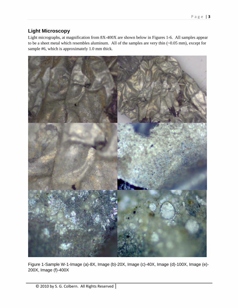
Light micrographs, at magnification from 8X-400X are shown below in Figures 1-6. All samples appear
to be a sheet metal which resembles aluminum. All of the samples are very thin (~0.05 mm), except for
sample #6, which is approximately 1.0 mm thick.
Figure 1-Sample W-1-Image (a)-8X, Image (b)-20X, Image (c)-40X, Image (d)-100X, Image (e)-
200X, Image (f)-400X

P a g e | 4
© 2010 by S. G. Colbern. All Rights Reserved
Samples #2, #3, and #6 had thin surface coatings, which appeared to be a few microns in thickness.
These coatings later proved to be of different composition than the bulk metals.
These coatings could be removed by scraping with a knife, or other metallic instrument, but were bonded
fairly well to the metal (Figure 2). Samples W-2 and W-6 appeared to have the thickest coatings.
Figure 2-Sample W-2-Image (a)-40X, Image (b)-40X-Showing Coating Removed, Image (c)-
100X, Image (d)-200X, Image (e)-400X, Image (f)-100X
P a g e | 5
© 2010 by S. G. Colbern. All Rights Reserved
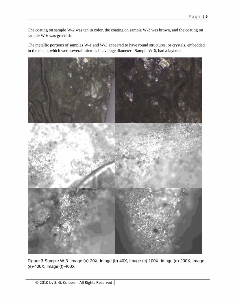
The coating on sample W-2 was tan in color, the coating on sample W-3 was brown, and the coating on
sample W-6 was greenish.
The metallic portions of samples W-1 and W-3 appeared to have round structures, or crystals, embedded
in the metal, which were several microns in average diameter. Sample W-6, had a layered
Figure 3-Sample W-3- Image (a)-20X, Image (b)-40X, Image (c)-100X, Image (d)-200X, Image
(e)-400X, Image (f)-400X
P a g e | 6
© 2010 by S. G. Colbern. All Rights Reserved
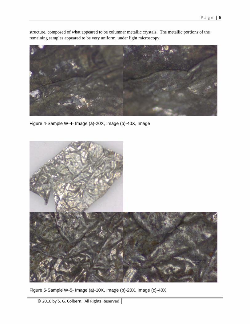
structure, composed of what appeared to be columnar metallic crystals. The metallic portions of the
remaining samples appeared to be very uniform, under light microscopy.
Figure 4-Sample W-4- Image (a)-20X, Image (b)-40X, Image
Figure 5-Sample W-5- Image (a)-10X, Image (b)-20X, Image (c)-40X

P a g e | 7
© 2010 by S. G. Colbern. All Rights Reserved
Figure 6-Sample W-6- Image (a)-10X, Image (b)-40X, Image (c)-40X, Image-Edge (d)-100X,
Image-Coating (e)-200X-Coating, Image (f)-400X-Coating
SEM Imaging
Scanning electron microscope (SEM) images were taken of all of the samples, at magnification ranging
from 25X to 15,000X. Higher magnifications were not used because a problem was encountered in
P a g e | 8
© 2010 by S. G. Colbern. All Rights Reserved
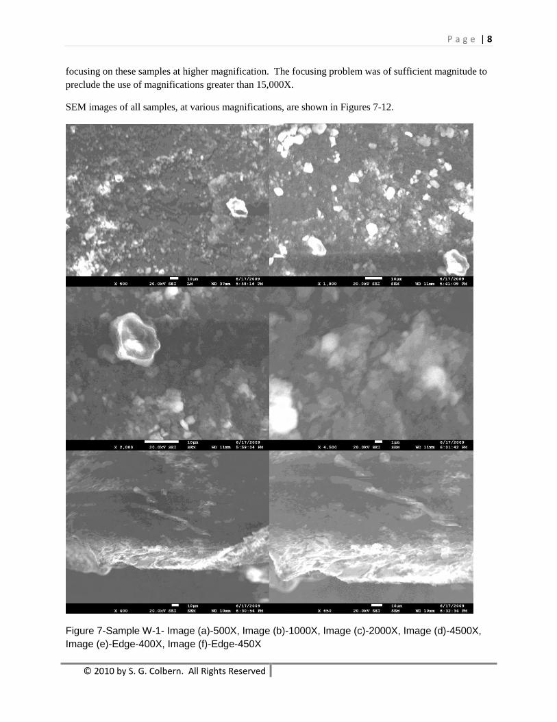
focusing on these samples at higher magnification. The focusing problem was of sufficient magnitude to
preclude the use of magnifications greater than 15,000X.
SEM images of all samples, at various magnifications, are shown in Figures 7-12.
Figure 7-Sample W-1- Image (a)-500X, Image (b)-1000X, Image (c)-2000X, Image (d)-4500X,
Image (e)-Edge-400X, Image (f)-Edge-450X
P a g e | 9
© 2010 by S. G. Colbern. All Rights Reserved
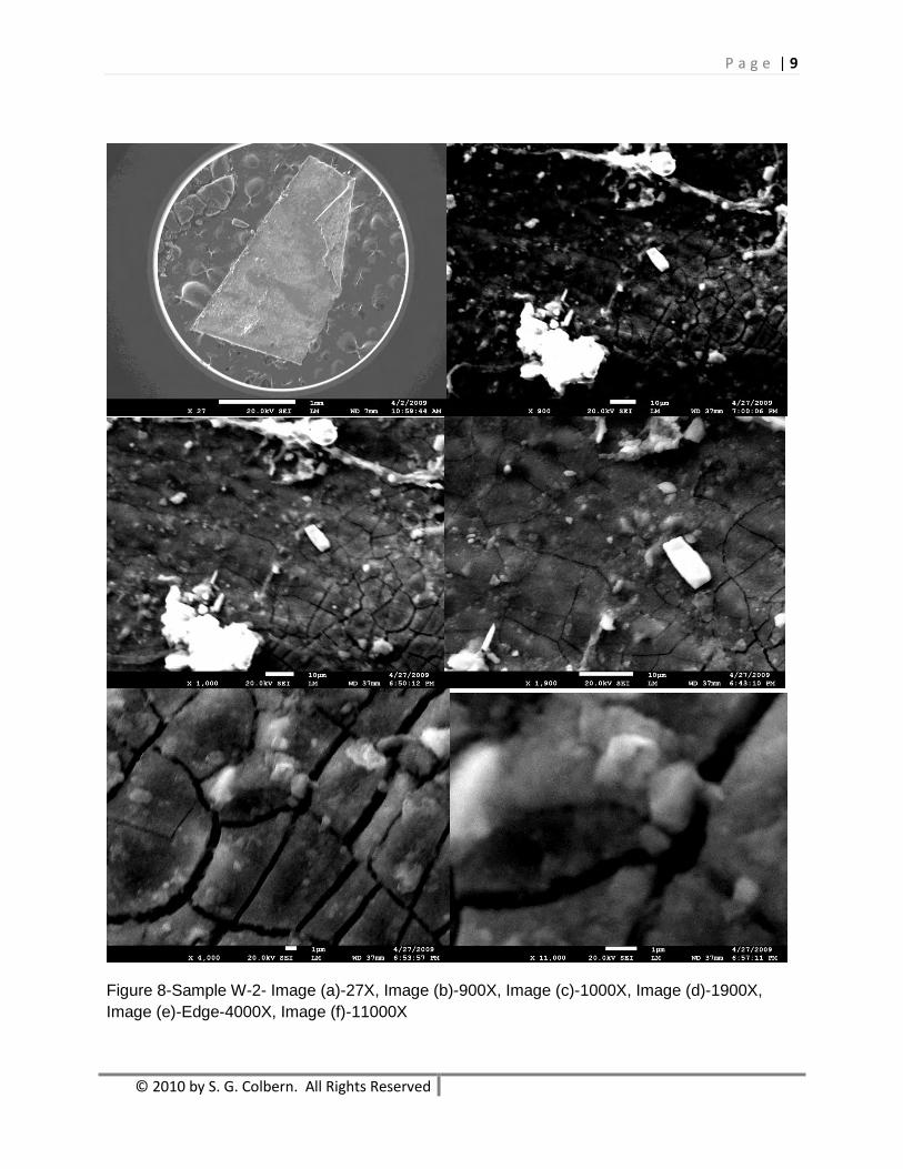
Figure 8-Sample W-2- Image (a)-27X, Image (b)-900X, Image (c)-1000X, Image (d)-1900X,
Image (e)-Edge-4000X, Image (f)-11000X

P a g e | 10
© 2010 by S. G. Colbern. All Rights Reserved
Figure 9-Sample W-3- Image (a)-1000X, Image (b)-2500X, Image (c)-5000X, Image (d)-7000X
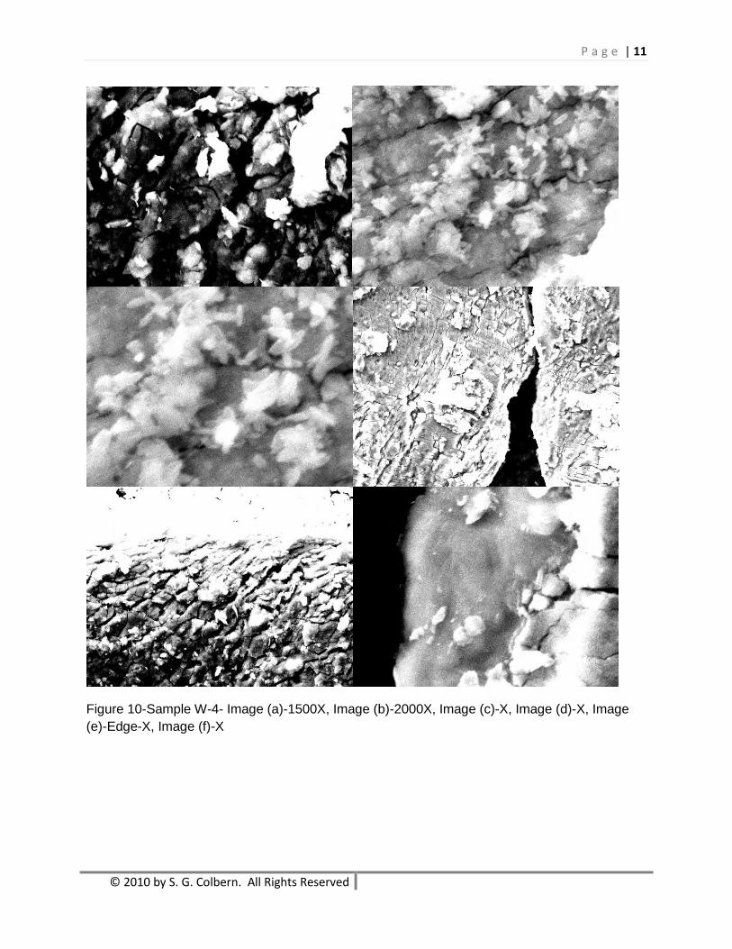
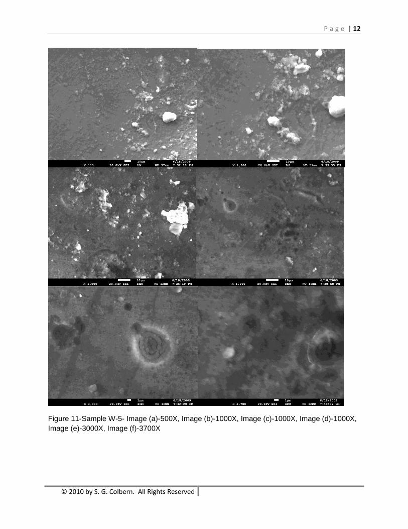
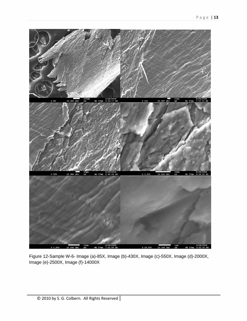
The SEM images showed ceramic-like crystals (Figures 7-11), cracks (Figures 8 and 10), and pits (Figure
11) in the outer coatings of the coated samples, and metallic crystals in the metallic portions of the
samples, especially sample W-6, which appeared to have a preferred direction to the metallic structure
(Figure 12).
P a g e | 11
© 2010 by S. G. Colbern. All Rights Reserved
Figure 10-Sample W-4- Image (a)-1500X, Image (b)-2000X, Image (c)-X, Image (d)-X, Image
(e)-Edge-X, Image (f)-X
P a g e | 12
© 2010 by S. G. Colbern. All Rights Reserved
Figure 11-Sample W-5- Image (a)-500X, Image (b)-1000X, Image (c)-1000X, Image (d)-1000X,
Image (e)-3000X, Image (f)-3700X
P a g e | 13
© 2010 by S. G. Colbern. All Rights Reserved
Figure 12-Sample W-6- Image (a)-85X, Image (b)-430X, Image (c)-550X, Image (d)-2000X,
Image (e)-2500X, Image (f)-14000X
P a g e | 14
© 2010 by S. G. Colbern. All Rights Reserved
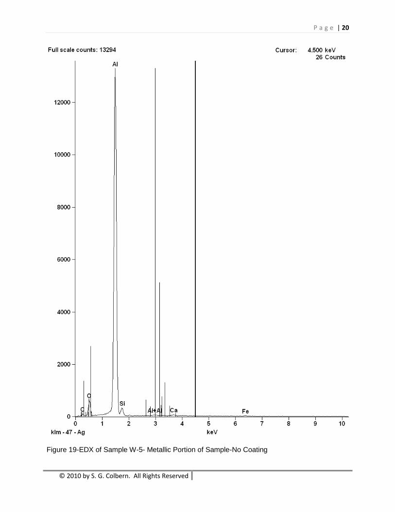
EDX Data
Energy Dispersive X-ray (EDX) elemental analysis was performed on all six Wade samples, in the course
of obtaining the SEM images. This analysis enables detection of elements present in relatively high
amounts, and gives the relative proportions of each.
EDX elemental mapping and point-and-shoot were done on selected sample areas, in addition to the
standard EDX spectra, which are elemental abundance averages over the area imaged. EDX mapping
shows a map of the relative concentrations of the elements detected in the imaged area, while EDX point-
and-shoot displays EDX spectra at selected points of an imaged area, highlighting differences in the
composition of imaged features.
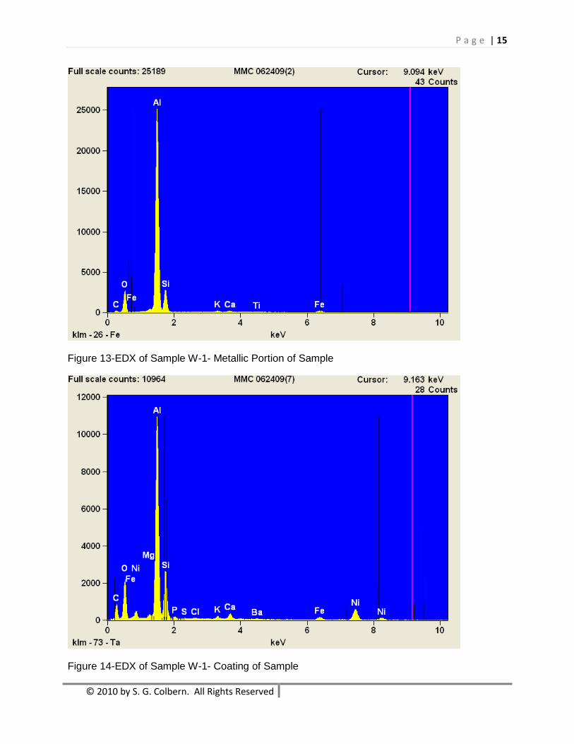
The major component of the metallic portions of all of the samples proved to be aluminum (Al). All of
the samples appeared to be composed of aluminum alloys, with varying amounts of alloying elements.
Other elements detected included beryllium (Be), carbon (C), oxygen (O), sodium (Na), magnesium
(Mg), silicon (Si), phosphorus (P), sulfur (S), chlorine (Cl), potassium (K), calcium (Ca), titanium (Ti),
iron (Fe), and palladium (Pd).
The coating layers of the coated samples were much different in composition from the metallic portions
of the samples. Aluminum was still a major component of the coatings, but was present to a lesser
degree than in the metallic portions of the samples.
The amount of oxygen in the coatings was much greater than in the metallic phase of the samples,
indicating that the aluminum was probably present as an oxide layer, rather than as free metal. The
proportions of carbon, silicon, and chlorine in the coatings were also higher than in the metal, indicating
the probable presence of metallic silicates, carbonates, and chlorides as components of the coatings.
All of the elements detected in the metallic phases were also present in the coatings. Some elements were
also present in the coatings which were not detected in the metallic phases; these included nickel (Ni), and
barium (Ba). The coatings of samples W-1 and W-6 were also quite similar to one another. The coatings
on samples W-2 and W-3 had not been analyzed by SEM/EDX as of the date of this report, but may be in
the near future.
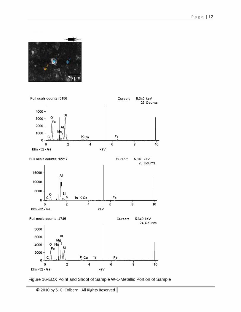
The EDX mapping of the coating of sample W-1 indicated that the oxygen, silicon, potassium, calcium,
and carbon in the coating tend to be concentrated in particles on the surface, which appear lighter in the
SEM images (Figure 15). The EDX point-and-shoot technique confirmed this (Figure 16). The majority
of the darker coating surface appears to consist of aluminum oxide.
P a g e | 15
© 2010 by S. G. Colbern. All Rights Reserved
Figure 13-EDX of Sample W-1- Metallic Portion of Sample
Figure 14-EDX of Sample W-1- Coating of Sample

P a g e | 16
© 2010 by S. G. Colbern. All Rights Reserved
Figure 15-EDX Mapping of Sample W-1- Metallic Portion of Sample
P a g e | 17
© 2010 by S. G. Colbern. All Rights Reserved
Figure 16-EDX Point and Shoot of Sample W-1-Metallic Portion of Sample
P a g e | 18
© 2010 by S. G. Colbern. All Rights Reserved
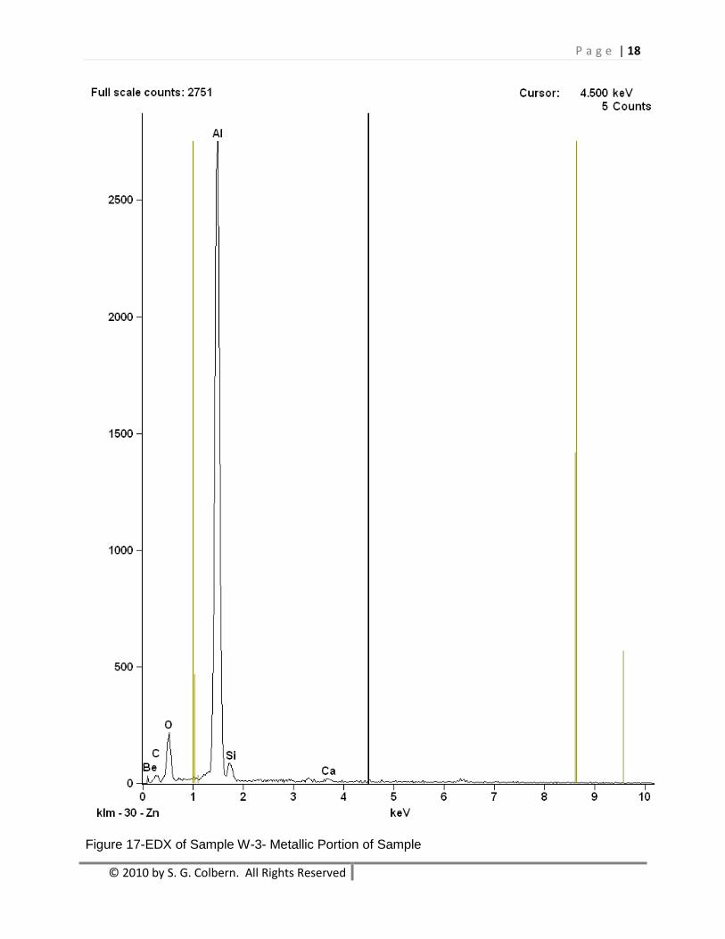
Figure 17-EDX of Sample W-3- Metallic Portion of Sample
P a g e | 19
© 2010 by S. G. Colbern. All Rights Reserved
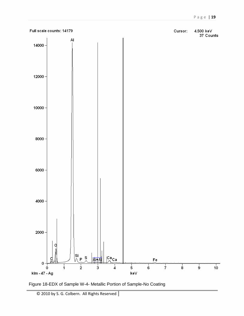
Figure 18-EDX of Sample W-4- Metallic Portion of Sample-No Coating
P a g e | 20
© 2010 by S. G. Colbern. All Rights Reserved
Figure 19-EDX of Sample W-5- Metallic Portion of Sample-No Coating

P a g e | 21
© 2010 by S. G. Colbern. All Rights Reserved
Figure 20-EDX of Sample W-6- Metallic Portion of Sample
Figure 21-EDX of Sample W-6- Coating Portion of Sample

P a g e | 22
© 2010 by S. G. Colbern. All Rights Reserved
Magnetic and Electrical Analysis
None of the samples were attracted to a strong Neodymium-Iron-Boron magnet, and are
therefore not ferromagnetic.
All of the samples were tested with a volt-ohmmeter, and were found to conduct electricity.
Quantitative values of sample resistivities will be determined when more of each sample is
available.
Raman Spectroscopy
Raman spectroscopy at 532 nm laser wavelength was carried out on the samples primarily to test for the
presence of carbon nanotubes, as this is a sensitive and reliable test for their presence in a material.
The presence of carbon nanotubes in the samples was suspected because of the previous detection of
carbon nanotubes in an alien implant sample, which was recently (2008) removed from the body of an
American materials scientist. Carbon nanotubes are currently being actively researched in Earthly
materials science because of their uniquely high strength-weight ratio, and electronic properties, and it
was hypothesized that much of the alien technology may utilize these materials.
The Raman data for all six samples is shown in Figures 22-24. The Raman wavenumber range which was
chosen for the analysis encompasses the range at which carbon nanotubes absorb laser radiation.
Figure 22-532 nm Raman Spectrum of all Wade Samples-Fullscale

P a g e | 23
© 2010 by S. G. Colbern. All Rights Reserved
Figure 23-532 nm Raman Spectrum of all Wade Samples-D and G Bands
Figure 24-532 nm Raman Spectrum of all Wade Samples-RBM Band
P a g e | 24
© 2010 by S. G. Colbern. All Rights Reserved
There are peaks in the spectra of all of the samples (Figures 22 and 24) which appear to be caused by the
presence of aluminum oxide (Al2O3, 110-116 cm-1
and 289-295 cm-1
), and the band structure of metallic
aluminum (Al, 522 cm-1
).
The Raman evidence for the presence of carbon nanotubes is inconclusive for samples W-2 through W-6.
Weak peaks appear in the area of 1200 cm-1
to 1600 cm-1
, which could be produced by single-walled
carbon nanotube D and G bands, but the signals are too weak to permit positive identification as such.
Sample W-1, however, does appear to have peaks that have a much higher probability of being caused by
the presence of single-walled carbon nanotube D (1381.7 cm-1
, 1448.7 cm-1
, and 1477.5 cm-1
) and G
bands (1539.6 cm-1
, 1589.9 cm-1
, and 1621.8 cm-1
, Figure 23).
ICP-MS Analysis
Pieces of all of the samples were subjected to trace element analysis by Inductively Coupled Plasma Mass
Spectroscopic (ICP-MS) analysis, performed by BodyCote testing lab, in Santa Fe Springs, CA.
This analysis involves dissolving small amounts of each sample (10 mg) in a mixture of nitric and
hydrochloric acids, and passing the solution through a plasma torch. The resulting plasma, containing
ions (charged atoms) of the elements in the sample are then passed through a mass spectrometer, which
sorts the ions by charge/mass ratio.
This analysis provides sensitive, and quantitative, results on the amounts of all elements present in the
sample. Amounts of most elements below parts-per-million (ppm) levels can be detected using this
analysis.
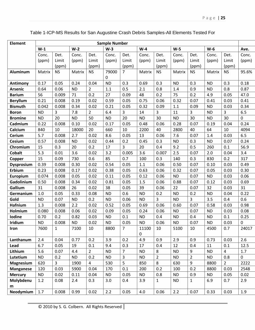
Sixty-eight (68) elements were tested for, with fifty-six (56) elements being detected in at least one
sample. The results of the analysis, with elements tested for in alphabetical order, are shown in Table 1.
The last column in the table is the average amount of each element detected for all six samples.
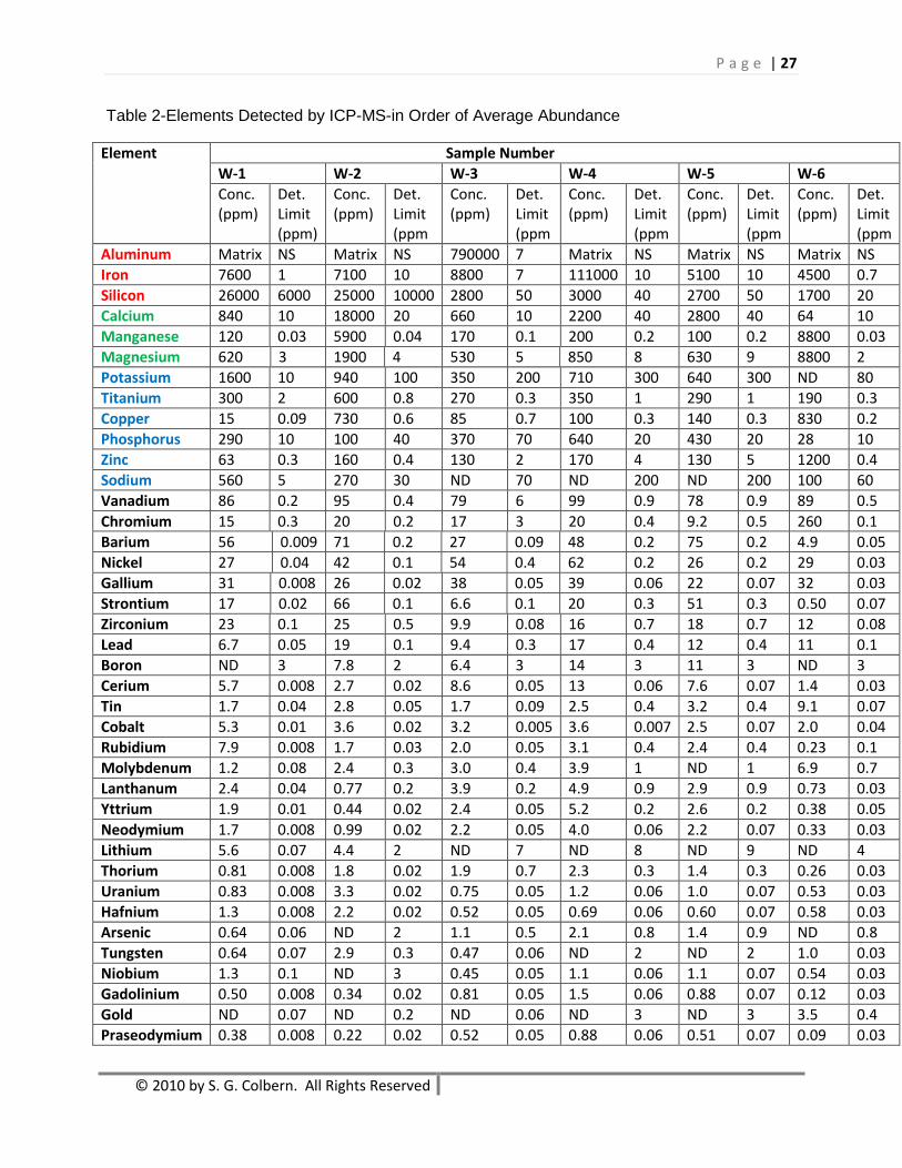
The results of the analysis, with elements listed in order of average abundance in all six samples, is shown
in Table 2.
Aluminum (Al, average concentration 95.6%) was the most abundant element in all of the samples,
followed by iron (Fe, ave. 2.40%), silicon (Si, ave. 1.02%), calcium (Ca, ave. 0.41%), manganese (Mn,
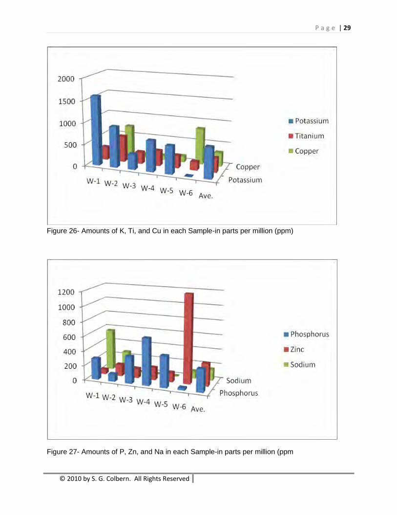
ave. 0.25%), magnesium (Mg, ave. 0.22%), potassium (K, ave. 0.07%; 707 ppm), titanium (Ti, ave.
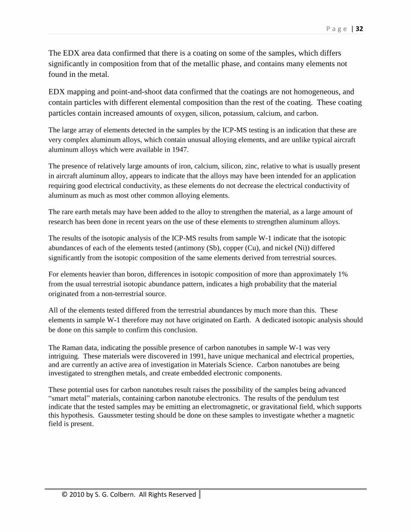
0.03%; 333 ppm), copper (Cu, ave. 0.03%; 317 ppm), phosphorus (P, ave. 0.03%; 310 ppm), zinc (Zn,
ave. 0.03%, 309 ppm), sodium (Na, 0.02; 155 ppm).
The amounts of the most abundant elements in the six samples varied widely with the specific sample,
implying differences in function. The amounts of the most abundant elements in the samples are shown
graphically in Figures 25-27.
The maximum, minimum, and average amounts of all of the elements in the samples are shown in Table 3
(See Appendix).
P a g e | 25
© 2010 by S. G. Colbern. All Rights Reserved
Table 1-ICP-MS Results for San Augustine Crash Debris Samples-All Elements Tested For
Element Sample Number
W-1 W-2 W-3 W-4 W-5 W-6 Ave.
Conc. (ppm)
Det. Limit (ppm)
Conc. (ppm)
Det. Limit (ppm)
Conc. (ppm)
Det. Limit (ppm)
Conc. (ppm)
Det. Limit (ppm)
Conc. (ppm)
Det. Limit (ppm)
Conc. (ppm)
Det. Limit (ppm)
Conc. (ppm)
Aluminum Matrix NS Matrix NS 790000
7 Matrix NS Matrix NS Matrix NS 95.6%
Antimony 0.17 0.05 0.24 0.04 ND 0.3 0.69 0.3 ND 0.3 ND 0.3 0.18
Arsenic 0.64 0.06 ND 2 1.1 0.5 2.1 0.8 1.4 0.9 ND 0.8 0.87
Barium 56 0.009 71 0.2 27 0.09 48 0.2 75 0.2 4.9 0.05 47.0
Beryllum 0.21 0.008 0.19 0.02 0.59 0.05 0.75 0.06 0.32 0.07 0.41 0.03 0.41
Bismuth 0.042 0.008 0.34 0.02 0.21 0.05 0.32 0.09 1.1 0.09 ND 0.03 0.34
Boron ND 3 7.8 2 6.4 3 14 3 11 3 ND 3 6.5
Bromine ND 20 ND 50 ND 20 ND 30 ND 30 ND 30 0
Cadmium 0.22 0.008 0.10 0.02 0.17 0.05 0.48 0.06 0.28 0.07 0.19 0.04 0.24
Calcium 840 10 18000 20 660 10 2200 40 2800 40 64 10 4094
Cerium 5.7 0.008 2.7 0.02 8.6 0.05 13 0.06 7.6 0.07 1.4 0.03 6.5
Cesium 0.57 0.008 ND 0.02 0.44 0.2 0.45 0.3 ND 0.3 ND 0.07 0.24
Chromium 15 0.3 20 0.2 17 3 20 0.4 9.2 0.5 260 0.1 56.9
Cobalt 5.3 0.01 3.6 0.02 3.2 0.005 3.6 0.007 2.5 0.07 2.0 0.04 3.4
Copper 15 0.09 730 0.6 85 0.7 100 0.3 140 0.3 830 0.2 317
Dysprosium 0.39 0.008 0.30 0.02 0.54 0.05 1.1 0.06 0.50 0.07 0.10 0.03 0.49
Erbium 0.23 0.008 0.17 0.02 0.38 0.05 0.63 0.06 0.32 0.07 0.05 0.03 0.30
Europium 0.074 0.008 0.05 0.02 0.11 0.05 0.12 0.06 ND 0.07 ND 0.03 0.06
Gadolinium 0.50 0.008 0.34 0.02 0.81 0.05 1.5 0.06 0.88 0.07 0.12 0.03 0.69
Gallium 31 0.008 26 0.02 38 0.05 39 0.06 22 0.07 32 0.03 31
Germanium 1.0 0.05 0.33 0.08 ND 0.6 ND 0.2 ND 0.2 ND 0.04 0.22
Gold ND 0.07 ND 0.2 ND 0.06 ND 3 ND 3 3.5 0.4 0.6
Hafnium 1.3 0.008 2.2 0.02 0.52 0.05 0.69 0.06 0.60 0.07 0.58 0.03 0.98
Holmium 0.080 0.008 0.06 0.02 0.09 0.05 0.24 0.06 ND 0.07 ND 0.03 0.08
Iodine 0.70 0.2 0.82 0.03 ND 0.1 ND 0.4 ND 0.4 ND 0.1 0.25
Iridium ND 0.008 ND 0.02 ND 0.05 ND 0.06 ND 0.07 ND 0.03 0
Iron 7600 1 7100 10 8800 7 111000
10 5100 10 4500 0.7 24017
Lanthanum 2.4 0.04 0.77 0.2 3.9 0.2 4.9 0.9 2.9 0.9 0.73 0.03 2.6
Lead 6.7 0.05 19 0.1 9.4 0.3 17 0.4 12 0.4 11 0.1 12.5
Lithium 5.6 0.07 4.4 2 ND 7 ND 8 ND 9 ND 4 1.7
Lutetium ND 0.2 ND 0.2 ND 3 ND 2 ND 2 ND 0.8 0
Magnesium 620 3 1900 4 530 5 850 8 630 9 8800 2 2222
Manganese 120 0.03 5900 0.04 170 0.1 200 0.2 100 0.2 8800 0.03 2548
Mercury ND 0.02 0.11 0.04 ND 0.05 ND 0.8 ND 0.9 ND 0.05 0.02
Molybdenum
1.2 0.08 2.4 0.3 3.0 0.4 3.9 1 ND 1 6.9 0.7 2.9
Neodymium 1.7 0.008 0.99 0.02 2.2 0.05 4.0 0.06 2.2 0.07 0.33 0.03 1.9

P a g e | 26
© 2010 by S. G. Colbern. All Rights Reserved
Nickel 27 0.04 42 0.1 54 0.4 62 0.2 26 0.2 29 0.03 40
Niobium 1.3 0.1 ND 3 0.45 0.05 1.1 0.06 1.1 0.07 0.54 0.03 0.7
Osmium ND 0.09 ND 0.02 ND 0.2 ND 0.2 ND 0.2 ND 0.03 0
Palladium ND 0.008 ND 0.02 ND 0.05 ND 1 ND 1 ND 3 0
Phosphorus 290 10 100 40 370 70 640 20 430 20 28 10 310
Platinum ND 0.2 ND 0.6 ND 0.4 ND 0.3 ND 0.3 0.13 0.06 0.02
Potassium 1600 10 940 100 350 200 710 300 640 300 ND 80 707
Praseodymium
0.38 0.008 0.22 0.02 0.52 0.05 0.88 0.06 0.51 0.07 0.09 0.03 0.50
Rhenium ND 0.008 ND 0.02 ND 0.05 ND 0.06 ND 0.07 ND 0.03 0
Rhodium ND 0.008 ND 0.02 ND 0.05 ND 0.1 ND 0.1 ND 0.05 0
Rubidium 7.9 0.008 1.7 0.03 2.0 0.05 3.1 0.4 2.4 0.4 0.23 0.1 2.9
Ruthenium ND 0.008 ND 0.02 ND 0.05 ND 0.06 ND 0.07 ND 0.03 0
Samarium 0.31 0.008 0.20 0.02 0.45 0.05 0.76 0.06 0.40 0.07 0.04 0.03 0.36
Selenium 0.30 0.2 ND 1 ND 3 ND 6 ND 7 ND 3 0.05
Silicon 26000 6000 25000 10000 2800 50 3000 40 2700 50 1700 20 10200
Silver ND 0.03 ND 0.1 0.21 0.05 0.17 0.1 0.36 0.1 0.31 0.1 0.18
Sodium 560 5 270 30 ND 70 ND 200 ND 200 100 60 155
Strontium 17 0.02 66 0.1 6.6 0.1 20 0.3 51 0.3 0.50 0.07 27
Tantalum ND 0.2 ND 3 ND 0.05 ND 0.2 ND 0.2 ND 0.03 0
Tellurium ND 0.09 ND 0.1 ND 0.4 ND 4 ND 5 ND 3 0
Thallium 0.26 0.1 0.51 0.3 0.21 0.1 ND 3 ND 3 ND 0.4 0.16
Thorium 0.81 0.008 1.8 0.02 1.9 0.7 2.3 0.3 1.4 0.3 0.26 0.03 1.4
Thulium 0.036 0.008 0.03 0.02 ND 0.05 0.11 0.06 ND 0.07 ND 0.03 0.03
Tin 1.7 0.04 2.8 0.05 1.7 0.09 2.5 0.4 3.2 0.4 9.1 0.07 3.5
Titanium 300 2 600 0.8 270 0.3 350 1 290 1 190 0.3 333
Tungsten 0.64 0.07 2.9 0.3 0.47 0.06 ND 2 ND 2 1.0 0.03 0.84
Uranium 0.83 0.008 3.3 0.02 0.75 0.05 1.2 0.06 1.0 0.07 0.53 0.03 1.3
Vanadium 86 0.2 95 0.4 79 6 99 0.9 78 0.9 89 0.5 88
Ytterbium 0.25 0.008 0.20 0.02 0.46 0.1 0.70 0.06 0.32 0.07 0.05 0.03 0.33
Yttrium 1.9 0.01 0.44 0.02 2.4 0.05 5.2 0.2 2.6 0.2 0.38 0.05 2.2
Zinc 63 0.3 160 0.4 130 2 170 4 130 5 1200 0.4 309
Zirconium 23 0.1 25 0.5 9.9 0.08 16 0.7 18 0.7 12 0.08 17
68 elements were analyzed for. 56 elements were detected in at least one sample. Elements analyzed
for and not detected in any samples: Bromine, Gold, Iridium, Lutetium, Osmium, Palladium, Rhenium,
Rhodium, Ruthenium, Tantalum, Tellurium
P a g e | 27
© 2010 by S. G. Colbern. All Rights Reserved
Table 2-Elements Detected by ICP-MS-in Order of Average Abundance
Element Sample Number
W-1 W-2 W-3 W-4 W-5 W-6
Conc. (ppm)
Det. Limit (ppm)
Conc. (ppm)
Det. Limit (ppm
Conc. (ppm)
Det. Limit (ppm
Conc. (ppm)
Det. Limit (ppm
Conc. (ppm)
Det. Limit (ppm
Conc. (ppm)
Det. Limit (ppm
Aluminum Matrix NS Matrix NS 790000 7 Matrix NS Matrix NS Matrix NS
Iron 7600 1 7100 10 8800 7 111000 10 5100 10 4500 0.7
Silicon 26000 6000 25000 10000 2800 50 3000 40 2700 50 1700 20
Calcium 840 10 18000 20 660 10 2200 40 2800 40 64 10
Manganese 120 0.03 5900 0.04 170 0.1 200 0.2 100 0.2 8800 0.03
Magnesium 620 3 1900 4 530 5 850 8 630 9 8800 2
Potassium 1600 10 940 100 350 200 710 300 640 300 ND 80
Titanium 300 2 600 0.8 270 0.3 350 1 290 1 190 0.3
Copper 15 0.09 730 0.6 85 0.7 100 0.3 140 0.3 830 0.2
Phosphorus 290 10 100 40 370 70 640 20 430 20 28 10
Zinc 63 0.3 160 0.4 130 2 170 4 130 5 1200 0.4
Sodium 560 5 270 30 ND 70 ND 200 ND 200 100 60
Vanadium 86 0.2 95 0.4 79 6 99 0.9 78 0.9 89 0.5
Chromium 15 0.3 20 0.2 17 3 20 0.4 9.2 0.5 260 0.1
Barium 56 0.009 71 0.2 27 0.09 48 0.2 75 0.2 4.9 0.05
Nickel 27 0.04 42 0.1 54 0.4 62 0.2 26 0.2 29 0.03
Gallium 31 0.008 26 0.02 38 0.05 39 0.06 22 0.07 32 0.03
Strontium 17 0.02 66 0.1 6.6 0.1 20 0.3 51 0.3 0.50 0.07
Zirconium 23 0.1 25 0.5 9.9 0.08 16 0.7 18 0.7 12 0.08
Lead 6.7 0.05 19 0.1 9.4 0.3 17 0.4 12 0.4 11 0.1
Boron ND 3 7.8 2 6.4 3 14 3 11 3 ND 3
Cerium 5.7 0.008 2.7 0.02 8.6 0.05 13 0.06 7.6 0.07 1.4 0.03
Tin 1.7 0.04 2.8 0.05 1.7 0.09 2.5 0.4 3.2 0.4 9.1 0.07
Cobalt 5.3 0.01 3.6 0.02 3.2 0.005 3.6 0.007 2.5 0.07 2.0 0.04
Rubidium 7.9 0.008 1.7 0.03 2.0 0.05 3.1 0.4 2.4 0.4 0.23 0.1
Molybdenum 1.2 0.08 2.4 0.3 3.0 0.4 3.9 1 ND 1 6.9 0.7
Lanthanum 2.4 0.04 0.77 0.2 3.9 0.2 4.9 0.9 2.9 0.9 0.73 0.03
Yttrium 1.9 0.01 0.44 0.02 2.4 0.05 5.2 0.2 2.6 0.2 0.38 0.05
Neodymium 1.7 0.008 0.99 0.02 2.2 0.05 4.0 0.06 2.2 0.07 0.33 0.03
Lithium 5.6 0.07 4.4 2 ND 7 ND 8 ND 9 ND 4
Thorium 0.81 0.008 1.8 0.02 1.9 0.7 2.3 0.3 1.4 0.3 0.26 0.03
Uranium 0.83 0.008 3.3 0.02 0.75 0.05 1.2 0.06 1.0 0.07 0.53 0.03
Hafnium 1.3 0.008 2.2 0.02 0.52 0.05 0.69 0.06 0.60 0.07 0.58 0.03
Arsenic 0.64 0.06 ND 2 1.1 0.5 2.1 0.8 1.4 0.9 ND 0.8
Tungsten 0.64 0.07 2.9 0.3 0.47 0.06 ND 2 ND 2 1.0 0.03
Niobium 1.3 0.1 ND 3 0.45 0.05 1.1 0.06 1.1 0.07 0.54 0.03
Gadolinium 0.50 0.008 0.34 0.02 0.81 0.05 1.5 0.06 0.88 0.07 0.12 0.03
Gold ND 0.07 ND 0.2 ND 0.06 ND 3 ND 3 3.5 0.4
Praseodymium 0.38 0.008 0.22 0.02 0.52 0.05 0.88 0.06 0.51 0.07 0.09 0.03

P a g e | 28
© 2010 by S. G. Colbern. All Rights Reserved
Dysprosium 0.39 0.008 0.30 0.02 0.54 0.05 1.1 0.06 0.50 0.07 0.10 0.03
Beryllum 0.21 0.008 0.19 0.02 0.59 0.05 0.75 0.06 0.32 0.07 0.41 0.03
Samarium 0.31 0.008 0.20 0.02 0.45 0.05 0.76 0.06 0.40 0.07 0.04 0.03
Bismuth 0.042 0.008 0.34 0.02 0.21 0.05 0.32 0.09 1.1 0.09 ND 0.03
Ytterbium 0.25 0.008 0.20 0.02 0.46 0.1 0.70 0.06 0.32 0.07 0.05 0.03
Erbium 0.23 0.008 0.17 0.02 0.38 0.05 0.63 0.06 0.32 0.07 0.05 0.03
Iodine 0.70 0.2 0.82 0.03 ND 0.1 ND 0.4 ND 0.4 ND 0.1
Cadmium 0.22 0.008 0.10 0.02 0.17 0.05 0.48 0.06 0.28 0.07 0.19 0.04
Cesium 0.57 0.008 ND 0.02 0.44 0.2 0.45 0.3 ND 0.3 ND 0.07
Germanium 1.0 0.05 0.33 0.08 ND 0.6 ND 0.2 ND 0.2 ND 0.04
Silver ND 0.03 ND 0.1 0.21 0.05 0.17 0.1 0.36 0.1 0.31 0.1
Antimony 0.17 0.05 0.24 0.04 ND 0.3 0.69 0.3 ND 0.3 ND 0.3
Thallium 0.26 0.1 0.51 0.3 0.21 0.1 ND 3 ND 3 ND 0.4
Holmium 0.080 0.008 0.06 0.02 0.09 0.05 0.24 0.06 ND 0.07 ND 0.03
Europium 0.074 0.008 0.05 0.02 0.11 0.05 0.12 0.06 ND 0.07 ND 0.03
Selenium 0.30 0.2 ND 1 ND 3 ND 6 ND 7 ND 3
Thulium 0.036 0.008 0.03 0.02 ND 0.05 0.11 0.06 ND 0.07 ND 0.03
Platinum ND 0.2 ND 0.6 ND 0.4 ND 0.3 ND 0.3 0.13 0.06
Mercury ND 0.02 0.11 0.04 ND 0.05 ND 0.8 ND 0.9 ND 0.05
Red denotes major component elements (100%-1%), green-minor component elements (10,000 ppm-
1,000 ppm) blue-major trace elements (1,000 ppm-100 ppm), black-minor trace elements (< 100 ppm).
Figure 25-Amounts of Fe, Si, Ca, Mn, and Mg in each Sample-in parts per million (ppm)
P a g e | 29
© 2010 by S. G. Colbern. All Rights Reserved
Figure 26- Amounts of K, Ti, and Cu in each Sample-in parts per million (ppm)
Figure 27- Amounts of P, Zn, and Na in each Sample-in parts per million (ppm

P a g e | 30
© 2010 by S. G. Colbern. All Rights Reserved
Isotopic Analysis of Sample W-1
Antimony (Sb), copper (Cu) and nickel (Ni) were the only elements present in the samples which were
suitable to perform isotopic abundance calculations on from the raw ICP-MS data.
These elements were suitable for this analysis because there are no analytical interferences with their
isotopes from other isotopes found in the samples.
The results of the isotopic abundance calculations for sample W-1 are shown in Table 3.
These results are very unusual, and show extremely skewed isotopic ratios in the three tested elements,
relative to the normal terrestrial amounts of the isotopes in each of these elements.
Table 3-Isotopic Ratios of Suitable Elements in Sample W-1
Element Isotope Sample Isotopic
Abundance (%)
Terrestrial Isotopic
Abundance (%)
Antimony Sb121 49.58 57.36
Sb123 50.42 42.64
Copper Cu63 48.84 69.15
Cu65 51.16 30.85
Nickel Ni58 35.31 68.08
Ni60 32.41 26.23
Ni61 ND 1.14
Ni62 32.28 3.63
Other Tests Performed
Samples W-1 and W-6 were placed on a flat surface, and a pendulum, constructed from a 4 oz lead
weight tied to an 18” long piece of monofilament nylon line was passed over the samples. When the
weight passed over the samples at close range (< 2”) the weight consistently showed a noticeable
deflection away from the sample.
These results are similar to those obtained from a similar test done on all six samples by Chuck Wade at
the 2010 UFO Congress, in Laughlin, NV.

P a g e | 31
© 2010 by S. G. Colbern. All Rights Reserved
Discussion
Appearance and Physical Characteristics of Samples
The samples are composed of aluminum alloy sheet, some of which are coated with what appears to be a
protective coating. The samples had some soil attached when first received, and had clearly been buried
at one time
The corrugations on W-2, W-3, W-4, and W-5 are reminiscent of the type of bending which can occur
from sudden shock, as in an aircraft crash, although it cannot be ruled out that the samples could have
been manufactured in this form.
The samples were composed aluminum alloys, all having a low content of copper, and with unusual
alloying/trace elements, many of which were unheard of as components of aluminum alloys in 1947, and
are unlikely to have been introduced during the aluminum manufacturing process in that era.
These facts are consistent with the material being debris from the crash of an aircraft, or spacecraft at the
San Augustine desert location. If the crash did occur in 1947, the material seems inconsistent with the
materials that were commercially available at that time, and are possibly too advanced to have been
produced by the technology of that time period.
The mechanical strength of the materials is not extraordinary, however, and seems well within the normal
limits of the strength of commercially available aluminum alloys. The materials could all be bent, torn,
and cut with relative ease.
It is not known where these samples came from in the structure of the craft, however, and it is possible
that they came from interior structures, which did not require extreme mechanical strength. If this is the
case, then samples from the exterior of the craft may show much more mechanical strength and
toughness.
The layer of ceramic-like material, seen on some of the samples (W-2, W-3, and W-6) under light
microscopy, is interesting, and appears to be some type of protective layer placed over the metal. This
type of technology was probably not available in 1947.
One of the materials (sample W-6) also appeared to have a layered structure, which is not typical of
commercial aluminum alloys.
The SEM images of the materials also show surface coatings on the samples, which appear to be applied,
and are not the simple aluminum oxide surface layer which forms naturally on standard aluminum alloys.
These coatings have pits, and pores of somewhat regular composition. There are also particles on the
surface which EDX indicated have different composition from the remainder of the coating.
The layered structure of sample W-6 is also very apparent in the SEM images. This type of structure is
not seen in aluminum alloys, and is more reminiscent of the structure seem in some titanium alloys, or a
more complex material, applied in layers by chemical vapor deposition, or some similar technique.
P a g e | 32
© 2010 by S. G. Colbern. All Rights Reserved
The EDX area data confirmed that there is a coating on some of the samples, which differs
significantly in composition from that of the metallic phase, and contains many elements not
found in the metal.
EDX mapping and point-and-shoot data confirmed that the coatings are not homogeneous, and
contain particles with different elemental composition than the rest of the coating. These coating
particles contain increased amounts of oxygen, silicon, potassium, calcium, and carbon.
The large array of elements detected in the samples by the ICP-MS testing is an indication that these are
very complex aluminum alloys, which contain unusual alloying elements, and are unlike typical aircraft
aluminum alloys which were available in 1947.
The presence of relatively large amounts of iron, calcium, silicon, zinc, relative to what is usually present
in aircraft aluminum alloy, appears to indicate that the alloys may have been intended for an application
requiring good electrical conductivity, as these elements do not decrease the electrical conductivity of
aluminum as much as most other common alloying elements.
The rare earth metals may have been added to the alloy to strengthen the material, as a large amount of
research has been done in recent years on the use of these elements to strengthen aluminum alloys.
The results of the isotopic analysis of the ICP-MS results from sample W-1 indicate that the isotopic
abundances of each of the elements tested (antimony (Sb), copper (Cu), and nickel (Ni)) differed
significantly from the isotopic composition of the same elements derived from terrestrial sources.
For elements heavier than boron, differences in isotopic composition of more than approximately 1%
from the usual terrestrial isotopic abundance pattern, indicates a high probability that the material
originated from a non-terrestrial source.
All of the elements tested differed from the terrestrial abundances by much more than this. These
elements in sample W-1 therefore may not have originated on Earth. A dedicated isotopic analysis should
be done on this sample to confirm this conclusion.
The Raman data, indicating the possible presence of carbon nanotubes in sample W-1 was very
intriguing. These materials were discovered in 1991, have unique mechanical and electrical properties,
and are currently an active area of investigation in Materials Science. Carbon nanotubes are being
investigated to strengthen metals, and create embedded electronic components.
These potential uses for carbon nanotubes result raises the possibility of the samples being advanced
“smart metal” materials, containing carbon nanotube electronics. The results of the pendulum test
indicate that the tested samples may be emitting an electromagnetic, or gravitational field, which supports
this hypothesis. Gaussmeter testing should be done on these samples to investigate whether a magnetic
field is present.
P a g e | 33
© 2010 by S. G. Colbern. All Rights Reserved
Conclusions 1) These samples contain very unusual alloying elements which were not present in aluminum
alloys in 1947. If these samples are from an aircraft which crashed in that year, they are very
unusual on that basis.
2) The coatings on the samples are also unusual because conformal coatings of this type, which are
blended with the metal, and rich in silica, titania, magnesia, sulfate, phosphate, and chloride, were
almost certainly not available in 1947. The coatings on the samples are also somewhat similar to
coatings on implants removed from people claiming alien contact.
3) The carbon nanotube indications observed in the Raman spectra of the samples indicates the
possibility that the samples may be “smart metal” materials, which contain carbon nanotubes as
electronic components, or to strengthen the materials. Since the mechanical strength of these
samples was not unusual, they should be tested for unusual electrical characteristics.
4) The isotopic ratios of three elements in sample W-1 (antimony, copper, and nickel) were
extremely skewed, with respect to the terrestrial ratios for these elements, and there is therefore a
high probability that the samples came from an extraterrestrial source. These extremely skewed
isotopic results are again reminiscent of those obtained from alleged alien implants, and from an
alleged piece of the Roswell crash debris which was analyzed by the late Dr. Russell
VernonClark (see appendix).
5) The results of the pendulum test indicate that samples W-1 and W-6 may still be emitting
gravitational, or magnetic energy, which greatly increases the probability these samples are
nanotechnological “smart metals” and of probable alien origin as well.
6) Further microscopic testing should be done on these materials to determine their internal
structures. More testing should also be done to determine the existence, extent, and profile of any
gravitational, magnetic, or electric fields the samples may be emitting, and their source of energy.
P a g e | 34
© 2010 by S. G. Colbern. All Rights Reserved
Appendix
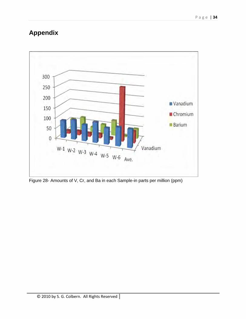
Figure 28- Amounts of V, Cr, and Ba in each Sample-in parts per million (ppm)
P a g e | 35
© 2010 by S. G. Colbern. All Rights Reserved
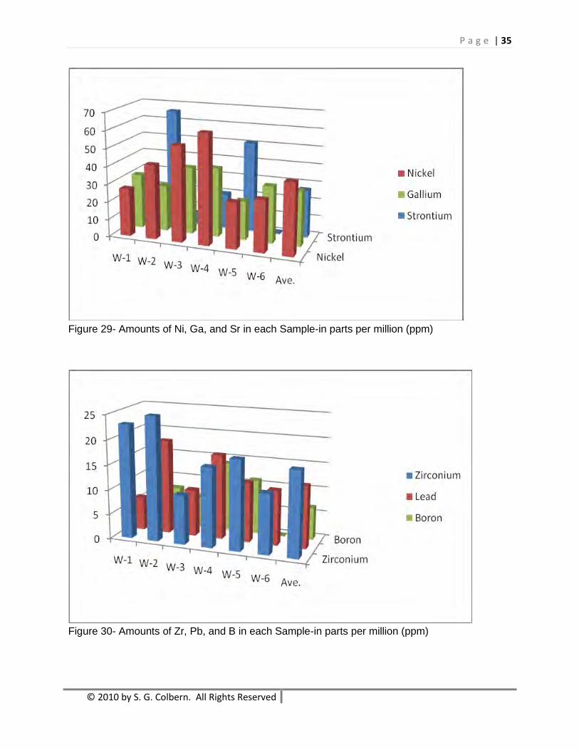
Figure 29- Amounts of Ni, Ga, and Sr in each Sample-in parts per million (ppm)
Figure 30- Amounts of Zr, Pb, and B in each Sample-in parts per million (ppm)
P a g e | 36
© 2010 by S. G. Colbern. All Rights Reserved
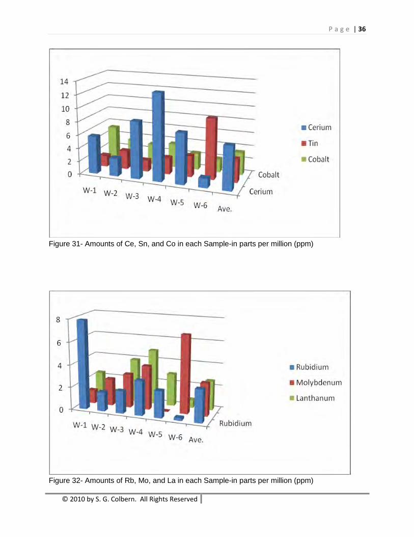
Figure 31- Amounts of Ce, Sn, and Co in each Sample-in parts per million (ppm)
Figure 32- Amounts of Rb, Mo, and La in each Sample-in parts per million (ppm)
P a g e | 37
© 2010 by S. G. Colbern. All Rights Reserved
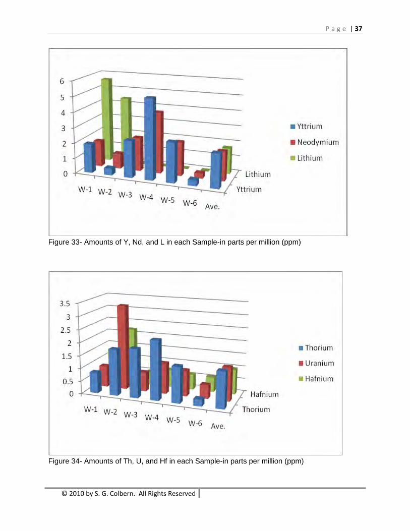
Figure 33- Amounts of Y, Nd, and L in each Sample-in parts per million (ppm)
Figure 34- Amounts of Th, U, and Hf in each Sample-in parts per million (ppm)
P a g e | 38
© 2010 by S. G. Colbern. All Rights Reserved
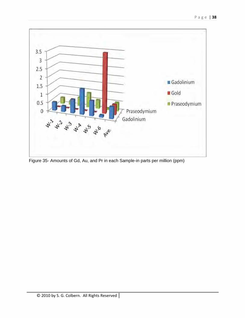
Figure 35- Amounts of Gd, Au, and Pr in each Sample-in parts per million (ppm)

P a g e | 39
© 2010 by S. G. Colbern. All Rights Reserved
Figure 36- Amounts of As, W, and Nb in each Sample-in parts per million (ppm)
Figure 37- Amounts of Dy, Be, and Sm in each Sample-in parts per million (ppm)

P a g e | 40
© 2010 by S. G. Colbern. All Rights Reserved
Figure 38- Amounts of Bi, Yb, and Er in each Sample-in parts per million (ppm)
Figure 39- Amounts of Ge, Ag, and Sb in each Sample-in parts per million (ppm)
P a g e | 41
© 2010 by S. G. Colbern. All Rights Reserved
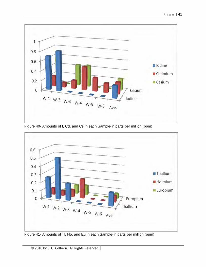
Figure 40- Amounts of I, Cd, and Cs in each Sample-in parts per million (ppm)
Figure 41- Amounts of Tl, Ho, and Eu in each Sample-in parts per million (ppm)
P a g e | 42
© 2010 by S. G. Colbern. All Rights Reserved
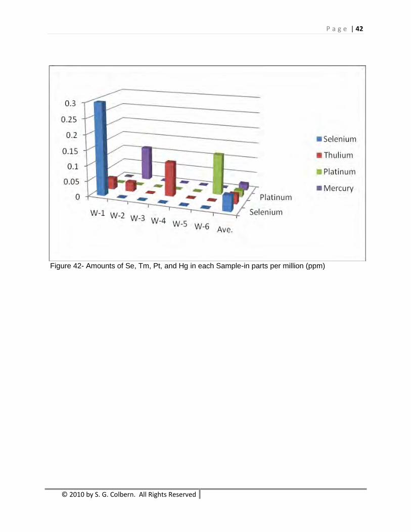
Figure 42- Amounts of Se, Tm, Pt, and Hg in each Sample-in parts per million (ppm)