In House Hi-Tech Testing Facility for Wads US Quality Control
Master’s DissertationStructural
Mechanics
PETER PERSSON
ANALYSIS OF VIBRATIONSIN HIGH-TECH FACILITY

Denna sida skall vara tom!
Copyright © 2010 by Structural Mechanics, LTH, Sweden.Printed by Wallin & Dalholm Digital AB, Lund, Sweden, June, 2010 (Pl).
For information, address:
Division of Structural Mechanics, LTH, Lund University, Box 118, SE-221 00 Lund, Sweden.Homepage: http://www.byggmek.lth.se
Structural MechanicsDepartment of Construction Sciences
Master’s Dissertation by
PETER PERSSON
Supervisor:
PhD Kent Persson,Div. of Structural Mechanics
ISRN LUTVDG/TVSM--10/5164--SE (1-73)ISSN 0281-6679
Examiner:
Associate Professor Delphine BardDiv. of Engineering Acoustics
ANALYSIS OF VIBRATIONS
IN HIGH-TECH FACILITY

Denna sida skall vara tom!
1
Preface
This master thesis was carried out at the Division of Structural Mechanics at LTH,Lund University, from October 2009 to May 2010.
First I would like to thank my supervisor Ph.D. Kent Persson, at the Division ofStructural Mechanics, for his great guidance and support during this work. Thismaster thesis would not have been possible without his help. I also would like tothank the sta� at the Division of Structural Mechanics and the sta� at MAX-labfor interesting and helpful discussions.
A special thanks to my father Ronny Persson for his great support and decisiveengagement during my entire education.
Lund, May 2010
Peter Persson

Denna sida skall vara tom!

3
Abstract
MAX-lab is a national synchrotron radiation facility in Lund. Nowadays, the MAXproject consist of three facilities (three storage rings). A new storage ring is neededto improve material science, such as nanotechnology. MAX IV, also in Lund, willbe 100 times more e�cient than already existing synchrotron radiation facilities.The storage ring is controlled by a large number of magnets that are distributedalong the ring. Since the quality of the measurement results from the MAX IV ringis dependent on the precision of the synchrotron light, a very strict requirementregarding the vibration levels of the magnets are de�ned. Vibration levels must beless than 26 nm during 1 s in the frequency span of 5-100 Hz. The site of MAX IVis located in an area in northeastern Lund called Brunnshög. At the site there issedimentary bedrock and the soil mostly consists of boulder clay. The �oor of theMAX IV building will mainly be constituted of a concrete structure. The inner andthe outer radius of the structure are approximately 70 m and 110 m respectivelyand the storage ring has a circumference of approximately 500 m. The roof reachesthe height of approximately 13 m.
The aim is to establish realistic �nite element models that predict vibrations on the�oor at the magnet foundation with high accuracy. The ultimate goal is to showhow the structure can be constructed to reduce the vibration levels and to checkthe ful�lment of the requirements. Vibrations are analysed by the �nite elementmethod. Steady-state analyses are performed to investigate vibrations at the magnetfoundations for varying parameters. Transient analyses are performed to comparethe results with the requirements by using realistic walking loads.
The geometry of the FE-model was chosen to include the main laboratory concrete�oor, the storage ring tunnel and the soil. Interfaces between building elements areassumed to have full interaction and since the structure is exposed to loads with lowmagnitude both the concrete and the soil were modeled as linear elastic isotropicmaterials.
A parameter study was performed to investigate the dynamic behavior of the struc-ture. The load was applied as a harmonic concentrated force positioned on the �oor,10 m from the outer boundary. A frequency sweep in the range of 0-40 Hz was madeto investigate the behavior of the structure at di�erent load frequencies. It wasconcluded that the low sti�ness of the soil was the main cause of the vibration levelsof the magnet foundations in the storage ring tunnel. To simulate the walking loadas realistic as possible, it was applied as a transient moving load. Analyses weremade for two load patterns on the concrete �oor corresponding to tangential andradial walking patterns. It was concluded that the vibration levels of the magnetfoundations generated by the walking load of one person exceeds the requirementswhen walking next to the storage ring tunnel. Even if the walking load is locatedseveral meters away from the tunnel walking loads, especially from groups of people,must be considered in the design process.

Denna sida skall vara tom!
Contents
1 Introduction 7
1.1 Background . . . . . . . . . . . . . . . . . . . . . . . . . . . . . . . . 71.2 Objective and method . . . . . . . . . . . . . . . . . . . . . . . . . . 111.3 Disposition . . . . . . . . . . . . . . . . . . . . . . . . . . . . . . . . 11
2 Materials 13
2.1 Concrete . . . . . . . . . . . . . . . . . . . . . . . . . . . . . . . . . . 132.2 Soil . . . . . . . . . . . . . . . . . . . . . . . . . . . . . . . . . . . . . 14
3 Vibration Theory 15
3.1 Introduction . . . . . . . . . . . . . . . . . . . . . . . . . . . . . . . . 153.2 Natural frequencies and mode shapes . . . . . . . . . . . . . . . . . . 163.3 Steady-State . . . . . . . . . . . . . . . . . . . . . . . . . . . . . . . . 183.4 Determine damping . . . . . . . . . . . . . . . . . . . . . . . . . . . . 19
3.4.1 Rayleigh damping . . . . . . . . . . . . . . . . . . . . . . . . . 193.5 Wavelength . . . . . . . . . . . . . . . . . . . . . . . . . . . . . . . . 213.6 RMS-value . . . . . . . . . . . . . . . . . . . . . . . . . . . . . . . . . 22
4 The Finite Element Method 23
4.1 Isoparametric �nite elements . . . . . . . . . . . . . . . . . . . . . . . 23
5 FE Model 27
5.1 Software . . . . . . . . . . . . . . . . . . . . . . . . . . . . . . . . . . 275.2 Geometry . . . . . . . . . . . . . . . . . . . . . . . . . . . . . . . . . 275.3 Mesh . . . . . . . . . . . . . . . . . . . . . . . . . . . . . . . . . . . . 28
5.3.1 3D-solid element . . . . . . . . . . . . . . . . . . . . . . . . . 285.4 Materials . . . . . . . . . . . . . . . . . . . . . . . . . . . . . . . . . 30
5.4.1 Concrete . . . . . . . . . . . . . . . . . . . . . . . . . . . . . . 305.4.2 Soil . . . . . . . . . . . . . . . . . . . . . . . . . . . . . . . . . 305.4.3 Rayleigh damping . . . . . . . . . . . . . . . . . . . . . . . . . 31
5.5 Loading . . . . . . . . . . . . . . . . . . . . . . . . . . . . . . . . . . 32
6 Modelling Results 33
6.1 Evaluation points . . . . . . . . . . . . . . . . . . . . . . . . . . . . . 336.2 Harmonic loading . . . . . . . . . . . . . . . . . . . . . . . . . . . . . 33
5
6 CONTENTS
6.2.1 Young's modulus of concrete . . . . . . . . . . . . . . . . . . . 346.2.2 Damping ratios . . . . . . . . . . . . . . . . . . . . . . . . . . 356.2.3 Thickness of the concrete �oor . . . . . . . . . . . . . . . . . . 376.2.4 Pillars . . . . . . . . . . . . . . . . . . . . . . . . . . . . . . . 396.2.5 Divided �oor . . . . . . . . . . . . . . . . . . . . . . . . . . . 426.2.6 General conclusion . . . . . . . . . . . . . . . . . . . . . . . . 43
6.3 Transient loading . . . . . . . . . . . . . . . . . . . . . . . . . . . . . 456.3.1 Human walking . . . . . . . . . . . . . . . . . . . . . . . . . . 456.3.2 Walking load . . . . . . . . . . . . . . . . . . . . . . . . . . . 466.3.3 Results . . . . . . . . . . . . . . . . . . . . . . . . . . . . . . . 46
7 Discussion and Suggestions for Further Work 51
A Plots of frequency sweeps 55
1
Introduction
1.1 Background
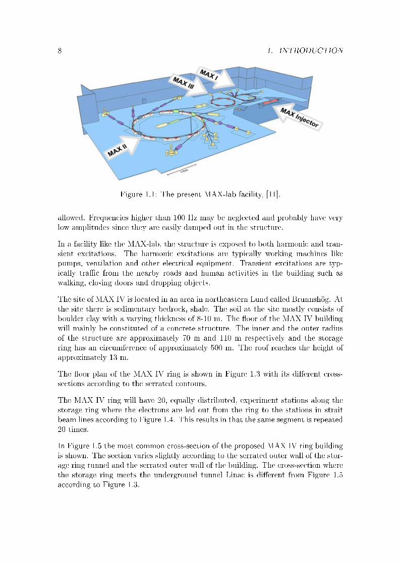
MAX-lab is a national laboratory in Lund operated jointly by the Swedish ResearchCouncil and Lund University. Nowadays, the MAX project consist of three facilities(three storage rings): MAX I, MAX II, MAX III and one electron pre-acceleratorcalled MAX Injector. In Figure 1.1 the present MAX-lab facility can be seen.
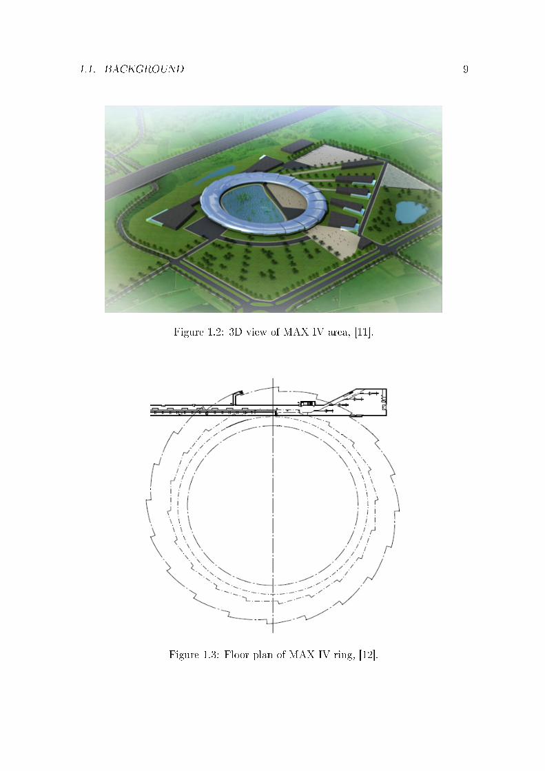
A new storage ring is needed to improve material science, such as nanotechnology.MAX IV, also in Lund, will be 100 times more e�cient than already existing syn-chrotron radiation facilities, e.g. it is planned to be the next generation Swedishsynchrotron radiation facility. MAX IV will basically consist of a main source thatwill be a 3 GeV ring with state-of-the-art low emittance for the production of softand hard x-rays as well as an expansion into the free electron laser �eld. The secondsource will be the Linac injector, an underground tunnel next to the main ring. TheLinac will provide short pulses to the main ring. In Figure 1.2 a 3D view of theMAX IV area can be seen.
In the storage ring the electrons are accelerated at high speeds. The particles thenemit electromagnetic radiation, so-called synchrotron light. The storage ring iscontrolled by a large number of magnets that are distributed along the ring. Themain concern is that vibrations at the magnets will give rise to a ten-fold increaseof the vibration of the electron beam. Since the quality of the measurement resultsfrom the MAX IV ring is dependent on the precision of the synchrotron light, avery strict requirement regarding the vibration levels of the magnets are speci�ed.The strict requirement is especially put on the mean vertical vibration level thatmust be less than 26 nm during one second in the frequency span of 5-100 Hz.Vibrations with frequencies lower than 5 Hz may be adjusted by an active calibrationsystem. In the interval between 0-5 Hz vibration levels up to 260 nm are therefore
7
8 1. INTRODUCTION
Figure 1.1: The present MAX-lab facility, [11].
allowed. Frequencies higher than 100 Hz may be neglected and probably have verylow amplitudes since they are easily damped out in the structure.
In a facility like the MAX-lab, the structure is exposed to both harmonic and tran-sient excitations. The harmonic excitations are typically working machines likepumps, ventilation and other electrical equipment. Transient excitations are typ-ically tra�c from the nearby roads and human activities in the building such aswalking, closing doors and dropping objects.
The site of MAX IV is located in an area in northeastern Lund called Brunnshög. Atthe site there is sedimentary bedrock, shale. The soil at the site mostly consists ofboulder clay with a varying thickness of 8-10 m. The �oor of the MAX IV buildingwill mainly be constituted of a concrete structure. The inner and the outer radiusof the structure are approximately 70 m and 110 m respectively and the storagering has an circumference of approximately 500 m. The roof reaches the height ofapproximately 13 m.
The �oor plan of the MAX IV ring is shown in Figure 1.3 with its di�erent cross-sections according to the serrated contours.
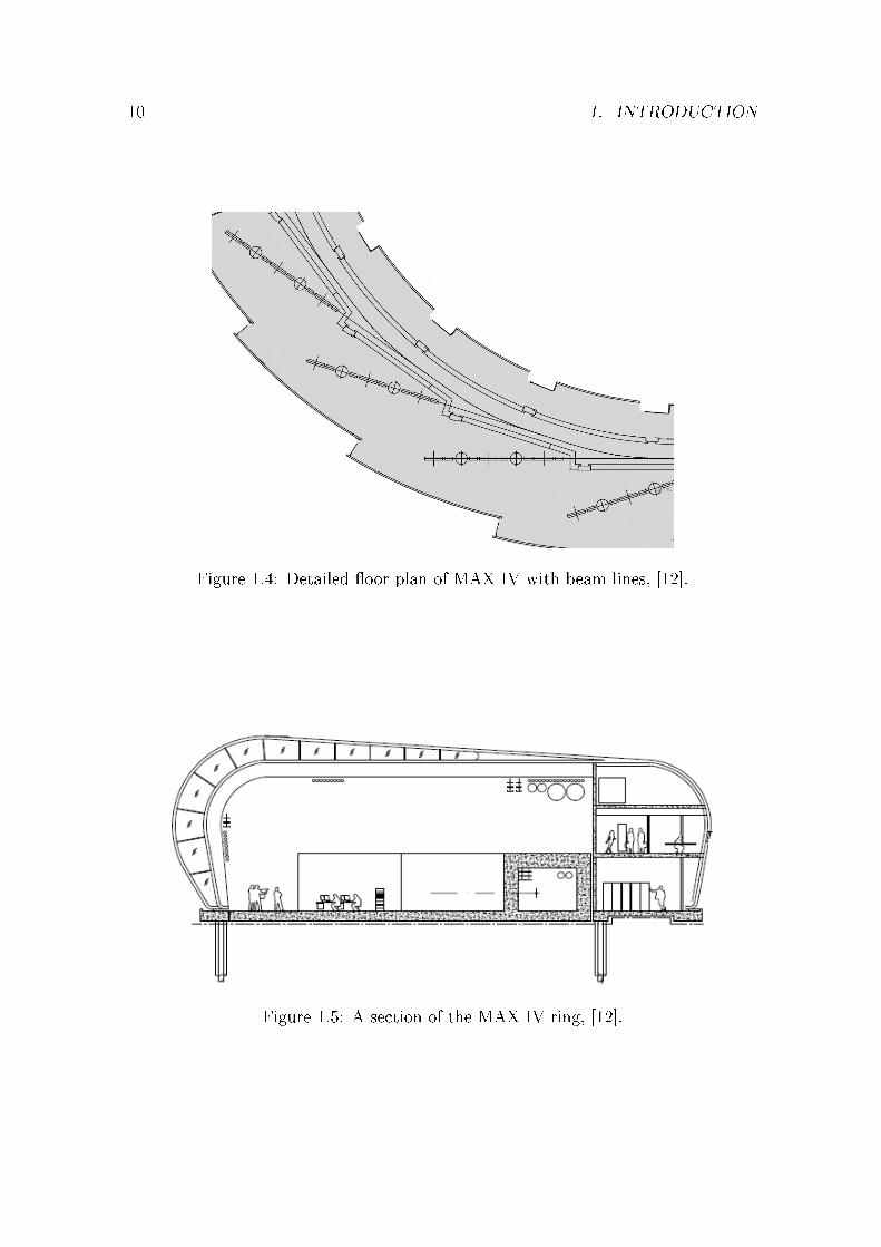
The MAX IV ring will have 20, equally distributed, experiment stations along thestorage ring where the electrons are led out from the ring to the stations in straitbeam lines according to Figure 1.4. This results in that the same segment is repeated20 times.
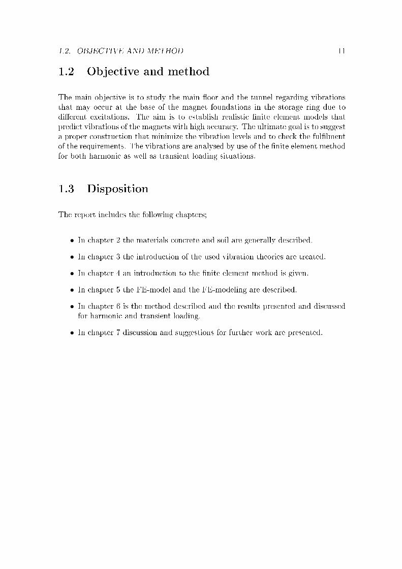
In Figure 1.5 the most common cross-section of the proposed MAX IV ring buildingis shown. The section varies slightly according to the serrated outer wall of the stor-age ring tunnel and the serrated outer wall of the building. The cross-section wherethe storage ring meets the underground tunnel Linac is di�erent from Figure 1.5according to Figure 1.3.
1.1. BACKGROUND 9
Figure 1.2: 3D view of MAX IV area, [11].
Figure 1.3: Floor plan of MAX IV ring, [12].
10 1. INTRODUCTION
Figure 1.4: Detailed �oor plan of MAX IV with beam lines, [12].
Figure 1.5: A section of the MAX IV ring, [12].
1.2. OBJECTIVE AND METHOD 11
1.2 Objective and method
The main objective is to study the main �oor and the tunnel regarding vibrationsthat may occur at the base of the magnet foundations in the storage ring due todi�erent excitations. The aim is to establish realistic �nite element models thatpredict vibrations of the magnets with high accuracy. The ultimate goal is to suggesta proper construction that minimize the vibration levels and to check the ful�lmentof the requirements. The vibrations are analysed by use of the �nite element methodfor both harmonic as well as transient loading situations.
1.3 Disposition
The report includes the following chapters;
• In chapter 2 the materials concrete and soil are generally described.
• In chapter 3 the introduction of the used vibration theories are treated.
• In chapter 4 an introduction to the �nite element method is given.
• In chapter 5 the FE-model and the FE-modeling are described.
• In chapter 6 is the method described and the results presented and discussedfor harmonic and transient loading.
• In chapter 7 discussion and suggestions for further work are presented.

Denna sida skall vara tom!
2
Materials
2.1 Concrete
Concrete is a composite that mainly consists of cement, sand, aggregate and water.With di�erent admixture the concrete can get various properties. When addingwater it reacts with cement and the concrete gets hardened. The process is calledhydration.
Hardened concrete has a density of 2400 kg/m3 and a Poisson's ratio of 0.2 accordingto [1]. A list of the characteristic values for Young's modulus for classi�ed concreteis presented in [1]. The characteristic value is the 5 % fractile of the statisticaldistribution. The values are in the range 27.0-39.0 GPa and is valid for static loading.For dynamic loading a multiplication factor of 1.2 should be used, [1]. The dampingratio for a concrete structure depends on the cracks, the joints, the reinforcementand the stress level. According to [3] the damping ratio for a concrete structure isin the range 2-10 % where the lower values corresponds to a well-reinforced concretestructure with low stress level and slight cracking. The most signi�cant property ofconcrete is that the tensile strength is just about 1/10 of the compressive strength.Tensile stresses can lead to cracking because of the low tensile strength.
To prevent the concrete's tendency to crack, reinforcement is used. The reinforce-ment is usually several reinforcing bars of steel that are placed out before the con-crete is casted. Forces are transferred between the concrete and the reinforcing barsby bonding and by contact pressure. There is also pre-stressed concrete where pre-stressed cables are used instead of or together with reinforcing bars. The pre-stressedcables contribute to an initial compressive stress of the concrete and therefore hasa higher capacity.
Concrete is the dominating construction material and is used in areas such as houses,plants, bridges, piles and foundations, [4].
13
14 2. MATERIALS
2.2 Soil
For more information about the material parameters of the soil and some of thefacts in this section, see [5] and [6].
Moraine covers about 75 % of Sweden's land area and is the most common soil typein Sweden. How the moraine is graded depends on what kind of bedrock there waspresent when it was formed. The moraine was formed when the ice sheets retreatedand erode the bedrock. In areas with sedimentary rocks, e.g. southwestern Scania,there is such a signi�cant amount of clay that is regarded as clay and called boulderclay. In areas with harder bedrock the moraine is more coarsely graded.
Strength and deformation properties of soil are a broad area with many uncertaintiesbecause of its varying composition. Parameters describing the deformation proper-ties of soil are often determined by laboratory tests and sometimes from in situ tests.Properties of moraine depend on the formation of the moraine and how the ice haspacked it. Moraine is therefore an unsorted and coarsely graded soil with varyingproperties.
Moraine is a very �rm soil with an undrained shear strength of over 100 kPa whereasfor boulder clay the undrained shear strength may be about 200-300 kPa. The stress-strain curve for a soft clay usually shows a linear behavior up to the preconsolidationpressure and in the overconsolidated state soil has mainly an elastic response uponunloading. Therefore soil is usually assumed to be linear elastic in overconsolidatedstate, i.e. at pressures lower than the preconsolidation pressure. Heavily overconsol-idated �ne graded soil and well compacted coarse graded soil show mainly an elasticresponse in shearing when exposed to loads with low magnitude. The soil at thesite of MAX IV is regarded as heavily overconcolidated due to the preconcolidationpressure is set to 400 kPa and it is exposed to vibration loads with low magnitude.
Clays often have a very low hydraulic conductivity i.e. its take time for clays todrain water during loading. Therefore the drained shear strength is only used whenit concerns long term loading, which implies that the undrained shear strength isused for the temporary loads such as tra�c, walking and impact.
Clays are usually water saturated. This results in that the density is the same fornatural moisture clay as water-saturated clay. The density for a clay is normallybetween 1400 and 2000 kg/m3 and for a boulder clay the density should be closerto 2000 kg/m3 because it is a coarsely graded soil. Since the clay normally iswater-saturated and water is incompressible the Poisson's ratio is often set to 0.5.The damping for soil, in this case boulder clay, is strain-dependent, i.e. the dampingincreases with the strain. Therefore the damping is set higher for earthquake analysisthan for analysis of very small vibration levels. The damping ratio could vary fromaround 1 to around 20 %.

3
Vibration Theory
3.1 Introduction
Vibrations occur in every building due to various kinds of loading. These loads varyin time and cause vibrations. There is a big di�erence between static and dynamicproblems. For static problems the solution follows the natural intuition, a biggerload needs a heavier structure to support the loads. For dynamic problems thefrequency of the load needs to be taken into account. If the frequency of the loadis close to a natural frequency of the system the displacements will become muchgreater than if the frequency of the load is far from a natural frequency.
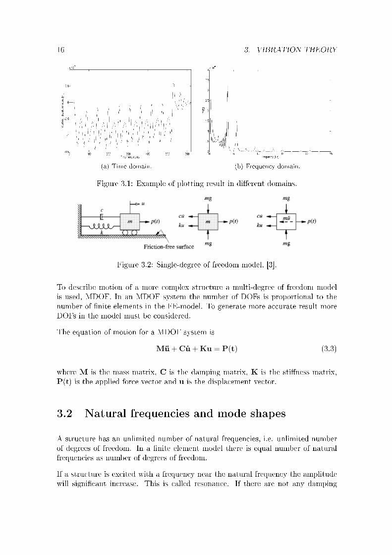
A dynamic event may be plotted in time domain or in frequency domain. In the timedomain the system is described as time dependent and in the frequency domain thesystem is described as frequency dependent. To convert a signal in the time domainto the frequency domain and vice versa, a "Fast Fourier Transform (FFT)" algorithmcan be used.
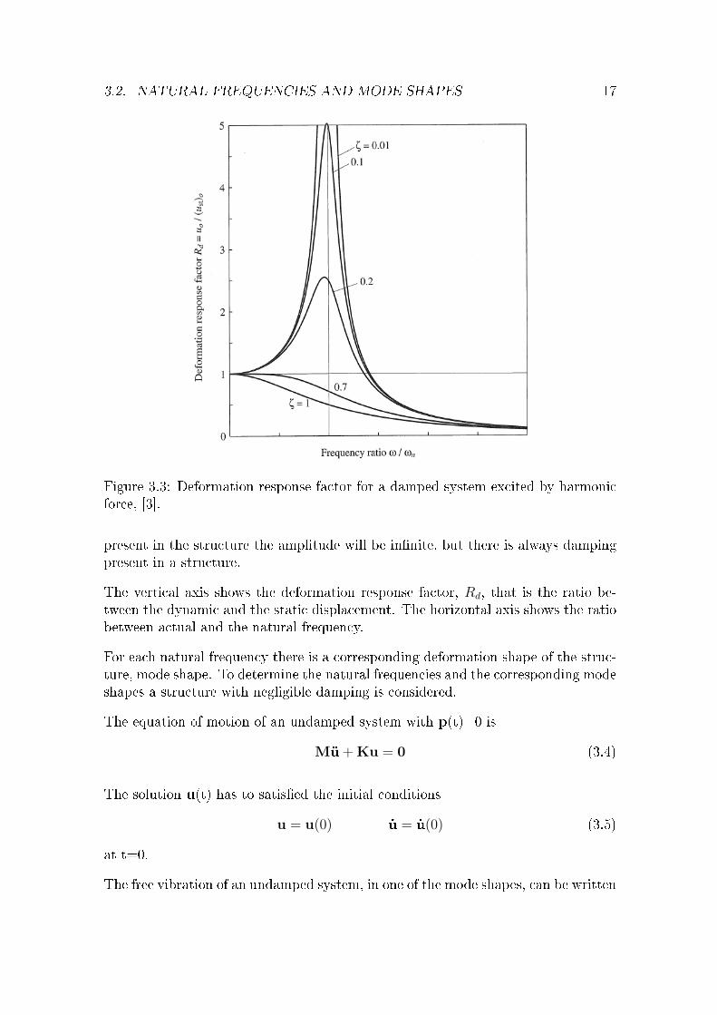
The easiest way to describe a dynamic system is by use of a single-degree of freedommodel, SDOF. An SDOF only contains one DOF meaning that it only needs oneDOF to describe the exact position of the mass. The system shown in Figure 3.2consists of a mass, a damper and a spring. The mass, m, is to be located in a pointand the displacement, u, is in one direction. The load p(t) is a time-dependentloading. The damper and the spring are regarded as mass-less.
Force equilibrium and Newton's second law gives
p(t)− c u − ku = mü (3.1)
and rewriting it to the equation of motion of a SDOF model
mü + c u + ku = p(t) (3.2)
15
16 3. VIBRATION THEORY
(a) Time domain. (b) Frequency domain.
Figure 3.1: Example of plotting result in di�erent domains.
Figure 3.2: Single-degree of freedom model, [3].
To describe motion of a more complex structure a multi-degree of freedom modelis used, MDOF. In an MDOF system the number of DOFs is proportional to thenumber of �nite elements in the FE-model. To generate more accurate result moreDOFs in the model must be considered.
The equation of motion for a MDOF system is
Mü+ C u+ Ku = P(t) (3.3)
where M is the mass matrix, C is the damping matrix, K is the sti�ness matrix,P(t) is the applied force vector and u is the displacement vector.
3.2 Natural frequencies and mode shapes
A structure has an unlimited number of natural frequencies, i.e. unlimited numberof degrees of freedom. In a �nite element model there is equal number of naturalfrequencies as number of degrees of freedom.
If a structure is excited with a frequency near the natural frequency the amplitudewill signi�cant increase. This is called resonance. If there are not any damping
3.2. NATURAL FREQUENCIES AND MODE SHAPES 17
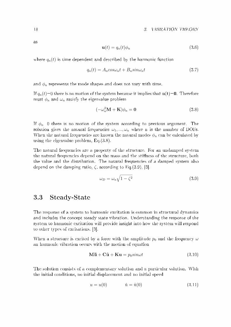
Figure 3.3: Deformation response factor for a damped system excited by harmonicforce, [3].
present in the structure the amplitude will be in�nite, but there is always dampingpresent in a structure.
The vertical axis shows the deformation response factor, Rd, that is the ratio be-tween the dynamic and the static displacement. The horizontal axis shows the ratiobetween actual and the natural frequency.
For each natural frequency there is a corresponding deformation shape of the struc-ture, mode shape. To determine the natural frequencies and the corresponding modeshapes a structure with negligible damping is considered.
The equation of motion of an undamped system with p(t)=0 is
Mü+ Ku = 0 (3.4)
The solution u(t) has to satis�ed the initial conditions
u = u(0) u = u(0) (3.5)
at t=0.
The free vibration of an undamped system, in one of the mode shapes, can be written
18 3. VIBRATION THEORY
asu(t) = qn(t)φn (3.6)
where qn(t) is time dependent and described by the harmonic function
qn(t) = Ancosωnt+Bnsinωnt (3.7)
and φn represents the mode shapes and does not vary with time.
If qn(t)=0 there is no motion of the system because it implies that u(t)=0. Thereforemust φn and ωn satisfy the eigenvalue problem
(−ω2nM + K)φn = 0 (3.8)
If φn=0 there is no motion of the system according to previous argument. Thesolution gives the natural frequencies ω1, ..., ωn where n is the number of DOFs.When the natural frequencies are known the natural modes φn can be calculated byusing the eigenvalue problem, Eq.(3.8).
The natural frequencies are a property of the structure. For an undamped systemthe natural frequencies depend on the mass and the sti�ness of the structure, boththe value and the distribution. The natural frequencies of a damped system alsodepend on the damping ratio, ζ, according to Eq.(3.9), [3].
ωD = ωn√
1− ζ2 (3.9)
3.3 Steady-State
The response of a system to harmonic excitation is common in structural dynamicsand includes the concept steady-state vibration. Understanding the response of thesystem to harmonic excitation will provide insight into how the system will respondto other types of excitations, [3].
When a structure is excited by a force with the amplitude p0 and the frequency ωan harmonic vibration occurs with the motion of equation
Mü+ C u+ Ku = p0sinωt (3.10)
The solution consists of a complementary solution and a particular solution. Withthe initial conditions, no initial displacement and no initial speed
u = u(0) u = u(0) (3.11)

3.4. DETERMINE DAMPING 19
the particular solution is
up(t) = Csinωt+Dcosωt (3.12)
and the complementary solution is
uc(t) = e−ξωnt(AcosωDt+BsinωDt) (3.13)
where A, B, C and D are integration constants.
The complete solution is then
u(t) = uc(t) + up(t) = e−ξωnt(AcosωDt+BsinωDt) + Csinωt+Dcosωt (3.14)
The solution contains two vibration components; transient vibration (complemen-tary solution) and steady-state vibration (particular solution). The transient vibra-tion decays exponentially with time towards zero. Then will only the steady-statevibration remains.
3.4 Determine damping
Damping is an e�ect that tends to reduce the vibration response in a structure.Damping is always present in a structure and arises for example from internal ma-terial damping and from friction in cracks and joints. Damping has a signi�cantin�uence on the response of a structure exposed to a dynamic force.
The damping properties cannot be calculated and should therefor be determinedusing measurements from similar structures. If there are not any appropriate mea-surements the damping matrix can be determined with di�erent procedures usingdamping ratios.
3.4.1 Rayleigh damping
For further reading about the Rayleigh damping method and for reference, see forexample [3].
Classical damping is an appropriate idealization if the mass and sti�ness are evenlydistributed through the structure. Rayleigh damping is a procedure to determinethe classical damping matrix with the use of damping ratios. It consists of twoparts; one is presupposing mass-proportionality and the other one is presupposing
20 3. VIBRATION THEORY
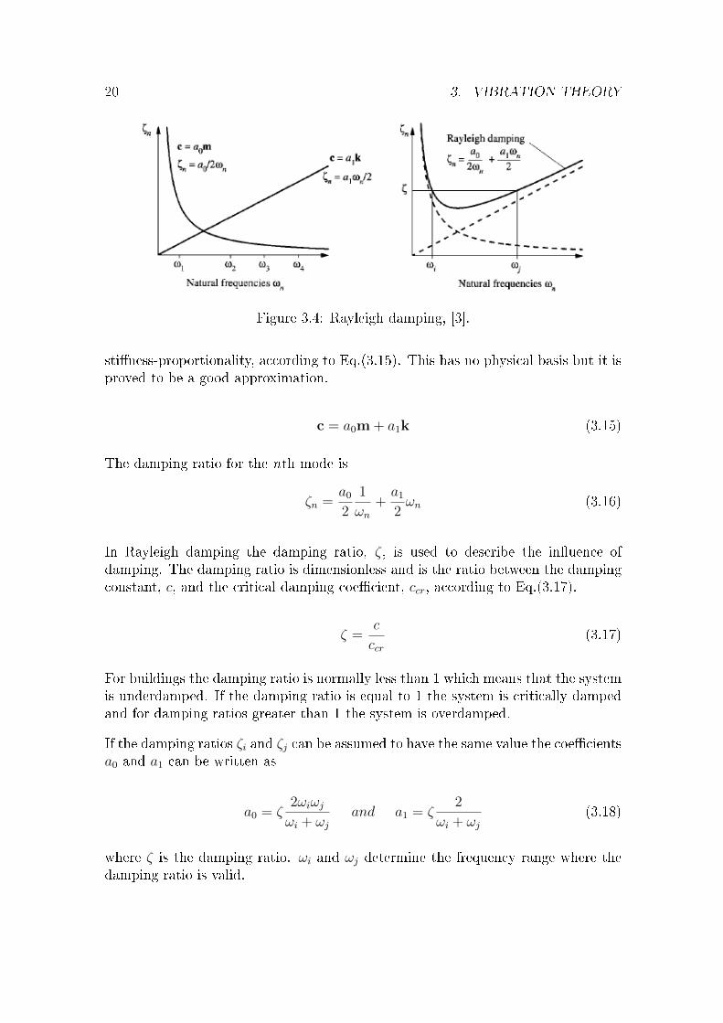
Figure 3.4: Rayleigh damping, [3].
sti�ness-proportionality, according to Eq.(3.15). This has no physical basis but it isproved to be a good approximation.
c = a0m + a1k (3.15)
The damping ratio for the nth mode is
ζn =a0
2
1
ωn+a1
2ωn (3.16)
In Rayleigh damping the damping ratio, ζ, is used to describe the in�uence ofdamping. The damping ratio is dimensionless and is the ratio between the dampingconstant, c, and the critical damping coe�cient, ccr, according to Eq.(3.17).
ζ =c
ccr(3.17)
For buildings the damping ratio is normally less than 1 which means that the systemis underdamped. If the damping ratio is equal to 1 the system is critically dampedand for damping ratios greater than 1 the system is overdamped.
If the damping ratios ζi and ζj can be assumed to have the same value the coe�cientsa0 and a1 can be written as
a0 = ζ2ωiωjωi + ωj
and a1 = ζ2
ωi + ωj(3.18)
where ζ is the damping ratio. ωi and ωj determine the frequency range where thedamping ratio is valid.
3.5. WAVELENGTH 21
In Figure 3.4 it is shown that the mass damps the lower frequencies and the sti�nessdamps the higher frequencies.
A soil-structure system is an example of a system with two or more parts withsigni�cantly di�erent damping ratios. The assumption of classical damping is notappropriate for this kind of systems but it is appropriate for each part separately.The damping matrix for the system, nonclassical damping matrix, is constructed byassembling the two classical damping matrixes, one for each part. It is appropriateto use Rayleigh damping for each part.
3.5 Wavelength
The wavelength is the distance over which the shape of the wave repeats itself.
The bending wave number for an isotropic plate is given by [13] as
k = (ω2ρh
EI)14 (3.19)
where ω is the angular frequency, ρ is the density, h is the height of the plate andEI is the bending sti�ness of the cross-section.
The bending wave number is also given by
k =2π
ω=ω
c(3.20)
Combining Eq.(3.19) and Eq.(3.20) the bending wave speed in an isotropic plate isgiven as
c =√ω 4
√EI
ρh(3.21)
The wave speed of a shear wave in an isotropic material is given by
c =
√G
ρ(3.22)
whereas the wave speed of a surface wave in an isotropic material is given by
c =
√E
ρ(3.23)
The relation between the wave speed, c, and the wavelength, λ is given by
λ =c
f(3.24)
where f is the frequency.
22 3. VIBRATION THEORY
3.6 RMS-value
RMS stands for Root Mean Square and is used as a measure of the magnitude of avibration. This is used instead of the mean value since the sign of the displacementsmay change during an analysis.
uRMS =
√1
∆t
∫ t0+∆t
t0u2(t)dt (3.25)
where u is the displacement amplitude and t is the time.
4
The Finite Element Method
For further reading about the �nite element method and for reference, see for ex-ample [2].
Di�erential equations are often used to describe various physical problems. Some-times di�erential equations are too complicated to be solved analytically insteadnumerical methods are required. Such a method is the �nite element method, FEM,that solves arbitrary boundary valued di�erential equations with arbitrary geome-tries and materials.
Development of FEM took o� in early 1960's and FEM is currently the most ef-fective method for solving arbitrary di�erential equations in engineering, physicsand mathematics. In order to solve di�erential equations with FEM the body isdivided into small elements, �nite elements. In FEM the variables of each elementis approximated. The body with the �nite elements is called a �nite element mesh.Every element has a relatively simple approximation, often a polynomial. At somepoints in the element the variables must be known, often at the boundary.
Since it is often tens of thousands of unknown degrees of freedom, the system ofequations cannot be solved without computer calculations. A �ner mesh, an there-fore an increased amount of DOFs, will normally generate a more accurate solution.
4.1 Isoparametric �nite elements
When modelling bodies with arbitrary geometries the �nite elements must be al-lowed to have curved boundaries, i.e. general shapes. Consider a cubic region in alocal ξηζ-coordinate system that is bounded by ξ=± 1, η=± 1 and ζ=± 1. Thelocal region is called the parent domain. This simple geometric shape in the localcoordinate system is mapped, transformed, into more a more complex geometry in
23
24 4. THE FINITE ELEMENT METHOD
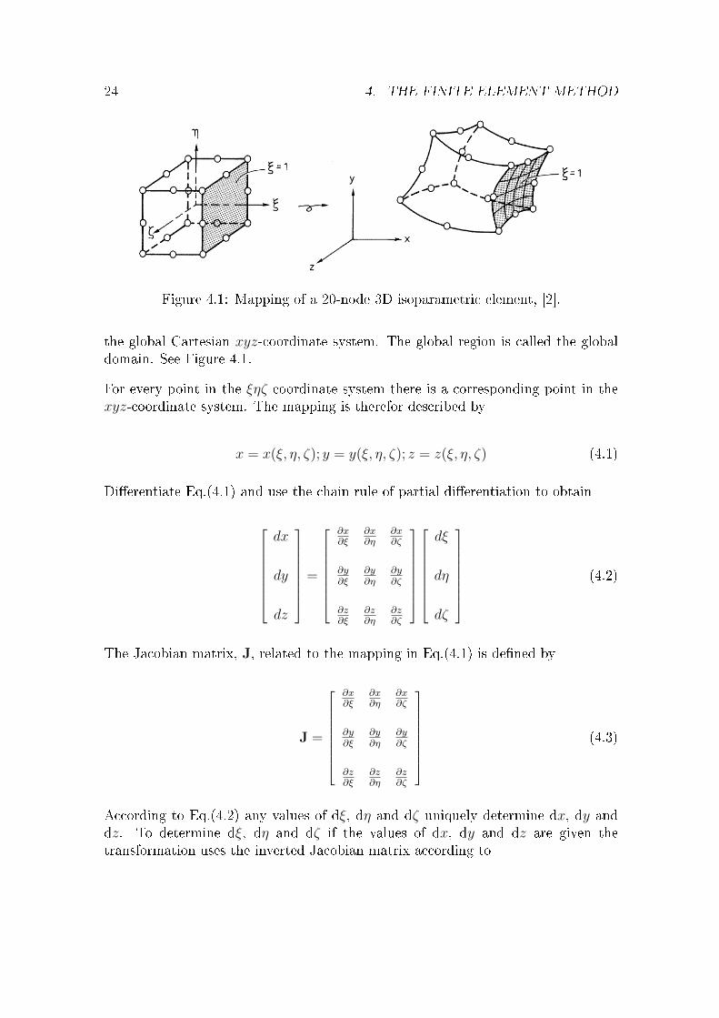
Figure 4.1: Mapping of a 20-node 3D isoparametric element, [2].
the global Cartesian xyz-coordinate system. The global region is called the globaldomain. See Figure 4.1.
For every point in the ξηζ-coordinate system there is a corresponding point in thexyz-coordinate system. The mapping is therefor described by
x = x(ξ, η, ζ); y = y(ξ, η, ζ); z = z(ξ, η, ζ) (4.1)
Di�erentiate Eq.(4.1) and use the chain rule of partial di�erentiation to obtain
dx
dy
dz
=
∂x∂ξ
∂x∂η
∂x∂ζ
∂y∂ξ
∂y∂η
∂y∂ζ
∂z∂ξ
∂z∂η
∂z∂ζ
dξ
dη
dζ
(4.2)
The Jacobian matrix, J, related to the mapping in Eq.(4.1) is de�ned by
J =
∂x∂ξ
∂x∂η
∂x∂ζ
∂y∂ξ
∂y∂η
∂y∂ζ
∂z∂ξ
∂z∂η
∂z∂ζ
(4.3)
According to Eq.(4.2) any values of dξ, dη and dζ uniquely determine dx, dy anddz. To determine dξ, dη and dζ if the values of dx, dy and dz are given thetransformation uses the inverted Jacobian matrix according to
4.1. ISOPARAMETRIC FINITE ELEMENTS 25
dξ
dη
dζ
= J−1
dx
dy
dz
(4.4)
Even if the mapping is unique it is not obtainable in the general case to invertEq.(4.1) into the explicit forms of ξ = ξ(x, y, z), η = η(x, y, z) and ζ = ζ(x, y, z).
To ful�ll the convergence requirement the compatibility and the completeness re-quirement must be satis�ed. If the element behaves compatible in the parent domainit will also do so in the global domain and the adjacent elements will match appro-priately. The completeness requirement is satis�ed if the sum of all values of theelement shape function at every node in the element is equal to 1, according toEq.(4.5).
n∑i=1
N ei = 1 (4.5)
To map an element from the parent domain to a global domain requires that thenodes on one element boundary in the parent domain also are located on one elementboundary in the global domain. It also requires that a corner node in one domainmust correspond to a corner node in the other domain, this also include the mid-sidenodes.

Denna sida skall vara tom!
5
FE Model
5.1 Software
The �nite element software Abaqus was used for the �nite element calculations.Abaqus is divided into three parts; Abaqus/CAE, Abaqus/Standard and Abaqus-/Explicit.
Abaqus/CAE is a user interface for modeling and meshing a structure and to visu-alize the results. Abaqus/Standard is an implicit solver for various dynamic �niteelement problems such as low-speed or steady-state analyses. Abaqus/Standard isalso used for static problems. Abaqus/Explicit use the explicit method and is moreappropriate for high-speed, nonlinear and transient response analyses.
In this investigationAbaqus/CAE was used for pre- and post processing andAbaqus-/Standard for the analyses.
5.2 Geometry
The geometry of the FE-model was chosen to include the main laboratory concrete�oor, the storage ring tunnel and the soil covering a radius of 150 m with a depthof 6 m. In Figure 5.1 a segment of the FE-model is shown. The segment is 1/20 ofthe whole model and this segment is repeated 20 times to produce the whole model.
The cross-section of MAX IV, shown in Figure 1.5, was somewhat simpli�ed to justincorporate the main �oor and the storage ring tunnel according to Figure 5.2. Theouter wall of the storage ring tunnel is still serrated as shown in Figure 1.3. Thedimension A shown in Figure 5.2 will therefore vary from 6-8 m.
27
28 5. FE MODEL
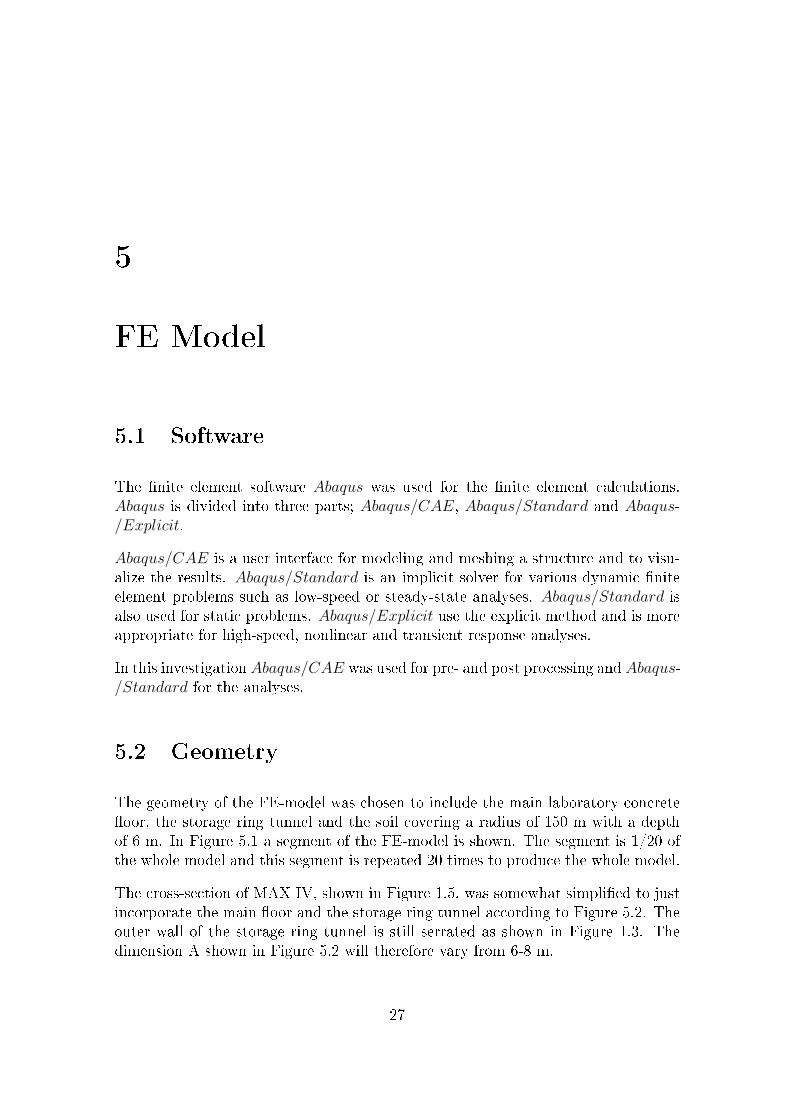
Figure 5.1: Segment of the FE-model.
Figure 5.2: Simply�ed section of the concrete structure.
The dimensions of the simpli�ed section were based on the architectural drawings.The inner and the outer radius of the modeled �oor were 80 m and 105 m, respec-tively. The radius of the storage ring was 83 m. The base thickness of the �oor was700 mm and the thickness of the walls of the storage ring tunnel was 1000 mm.
5.3 Mesh
The model was meshed with 36 761 3D-solid elements ending up at 572 178 degreesof freedom. The mesh of the soil was coarser than that of the concrete structure.
5.3.1 3D-solid element
3D-solid isoparametric elements were employed in the model. The elements were20-node quadratic brick elements, that is named C3D20R in Abaqus. C stands forcontinuum stress/displacement, 3D means that it is a tree-dimensional element, 20is the number of nodes and R means that reduced integration is used, [9]. Reducedintegration means that the order of integration is lower than when full integrationis used. Full integration provides a structure that is too sti� and therefore the
5.3. MESH 29
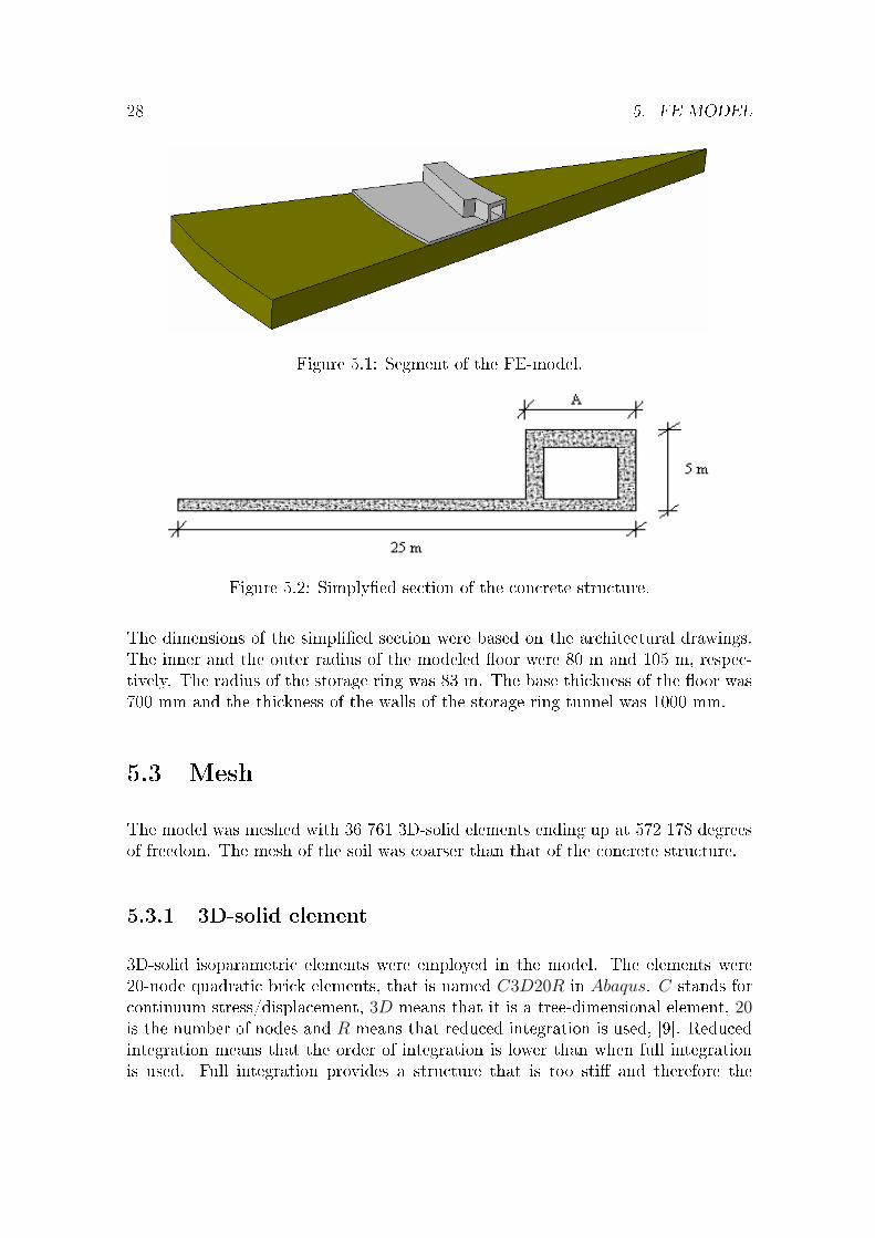
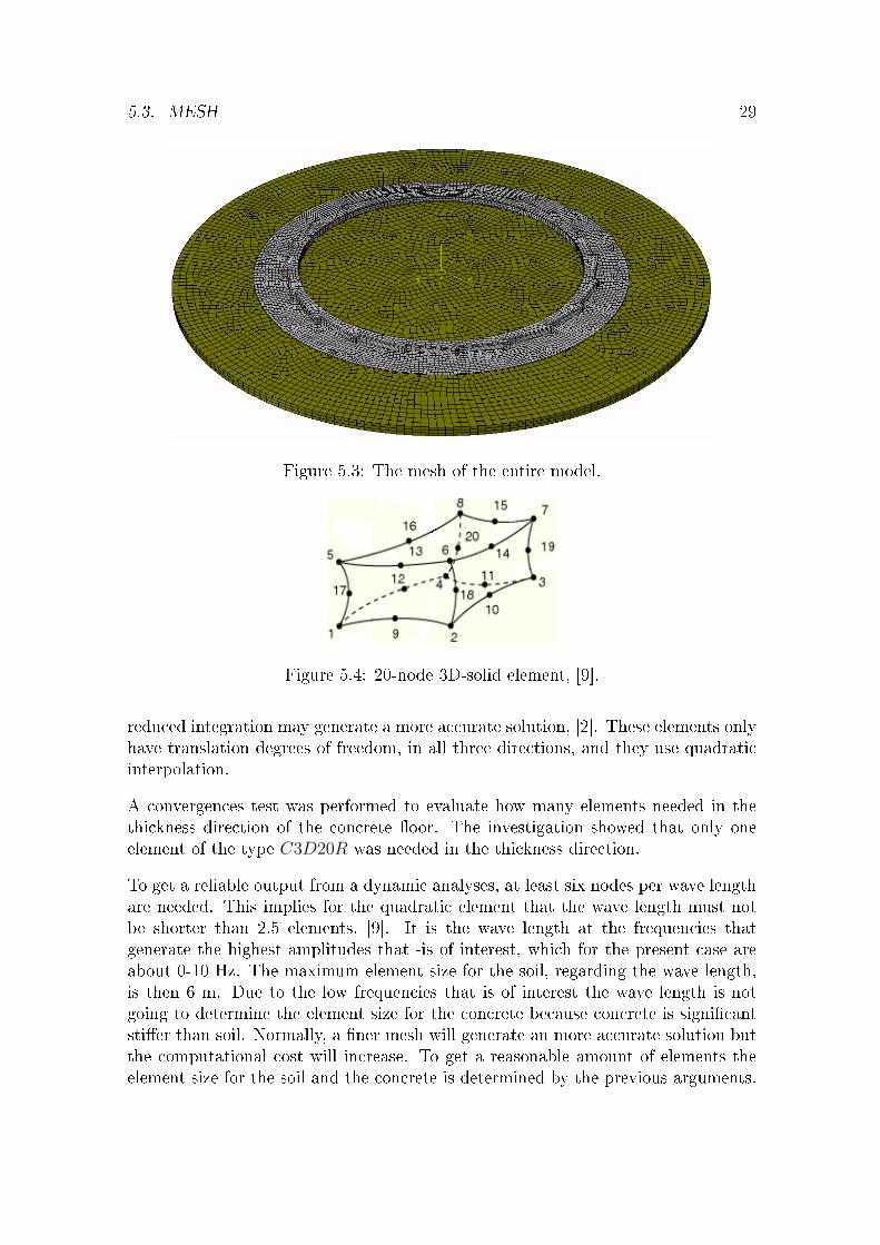
Figure 5.3: The mesh of the entire model.
Figure 5.4: 20-node 3D-solid element, [9].
reduced integration may generate a more accurate solution, [2]. These elements onlyhave translation degrees of freedom, in all three directions, and they use quadraticinterpolation.
A convergences test was performed to evaluate how many elements needed in thethickness direction of the concrete �oor. The investigation showed that only oneelement of the type C3D20R was needed in the thickness direction.
To get a reliable output from a dynamic analyses, at least six nodes per wave lengthare needed. This implies for the quadratic element that the wave length must notbe shorter than 2.5 elements, [9]. It is the wave length at the frequencies thatgenerate the highest amplitudes that -is of interest, which for the present case areabout 0-10 Hz. The maximum element size for the soil, regarding the wave length,is then 6 m. Due to the low frequencies that is of interest the wave length is notgoing to determine the element size for the concrete because concrete is signi�cantsti�er than soil. Normally, a �ner mesh will generate an more accurate solution butthe computational cost will increase. To get a reasonable amount of elements theelement size for the soil and the concrete is determined by the previous arguments.
30 5. FE MODEL
5.4 Materials
Since the structure is exposed to loads with low magnitude both the concrete and thesoil were modeled as linear elastic isotropic materials. Interfaces between buildingelements and between the structure and the soil are assumed to have full interaction.This means that the interfaces don't have any relative motion between them. Aset of base material parameters is speci�ed for the concrete and for the soil. Theparameters are the Young's modulus, E, the Poisson's ratio, ν, the density, ρ, andthe damping ratio, ζ.
5.4.1 Concrete
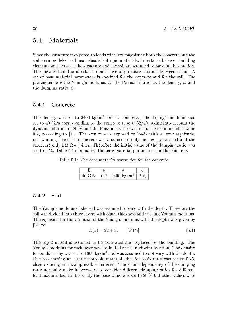
The density was set to 2400 kg/m3 for the concrete. The Young's modulus wasset to 40 GPa corresponding to the concrete type C 32/40 taking into account thedynamic addition of 20 % and the Poisson's ratio was set to the recommended value0.2, according to [1]. The structure is exposed to loads with a low magnitude,i.e. working stress, the concrete was assumed to only be slightly cracked and thestructure only has few joints. Therefore the initial value of the damping ratio wasset to 2 %. Table 5.1 summarize the base material parameters for the concrete.
Table 5.1: The base material parameter for the concrete.
E ν ρ ζ40 GPa 0.2 2400 kg/m3 2 %
5.4.2 Soil
The Young's modulus of the soil was assumed to vary with the depth. Therefore thesoil was divided into three layers with equal thickness and varying Young's modulus.The equation for the variation of the Young's modulus with the depth was given by[14] to
E(z) = 22 + 5z [MPa] (5.1)
The top 2 m soil is assumed to be excavated and replaced by the building. TheYoung's modulus for each layer was evaluated at the midpoint location. The densityfor boulder clay was set to 1800 kg/m3 and was assumed to not vary with the depth.Due to choosing an elastic isotropic material, the Poisson's ratio was set to 0.45,close to being an incompressible material. The strain dependency of the dampingratio normally make it necessary to consider di�erent damping ratios for di�erentload magnitudes. In this study the base value was set to 20 % but other values were
5.4. MATERIALS 31
also investigated. Table 5.2 summarize the base material parameters for the threelayers of soil.
Table 5.2: The base material parameter for the soil.
Layer E ν ρ ζ1 37 MPa 0.45 1800 kg/m3 20 %
2 47 MPa 0.45 1800 kg/m3 20 %
3 57 MPa 0.45 1800 kg/m3 20 %
The sedimentary bedrock, shale, beneath the soil was regarded as in�nite sti�. Con-sequently the bottom soil surface was constrained in the vertical direction. Moreover,in the horizontal directions only the rigid body motions were constrained.
5.4.3 Rayleigh damping
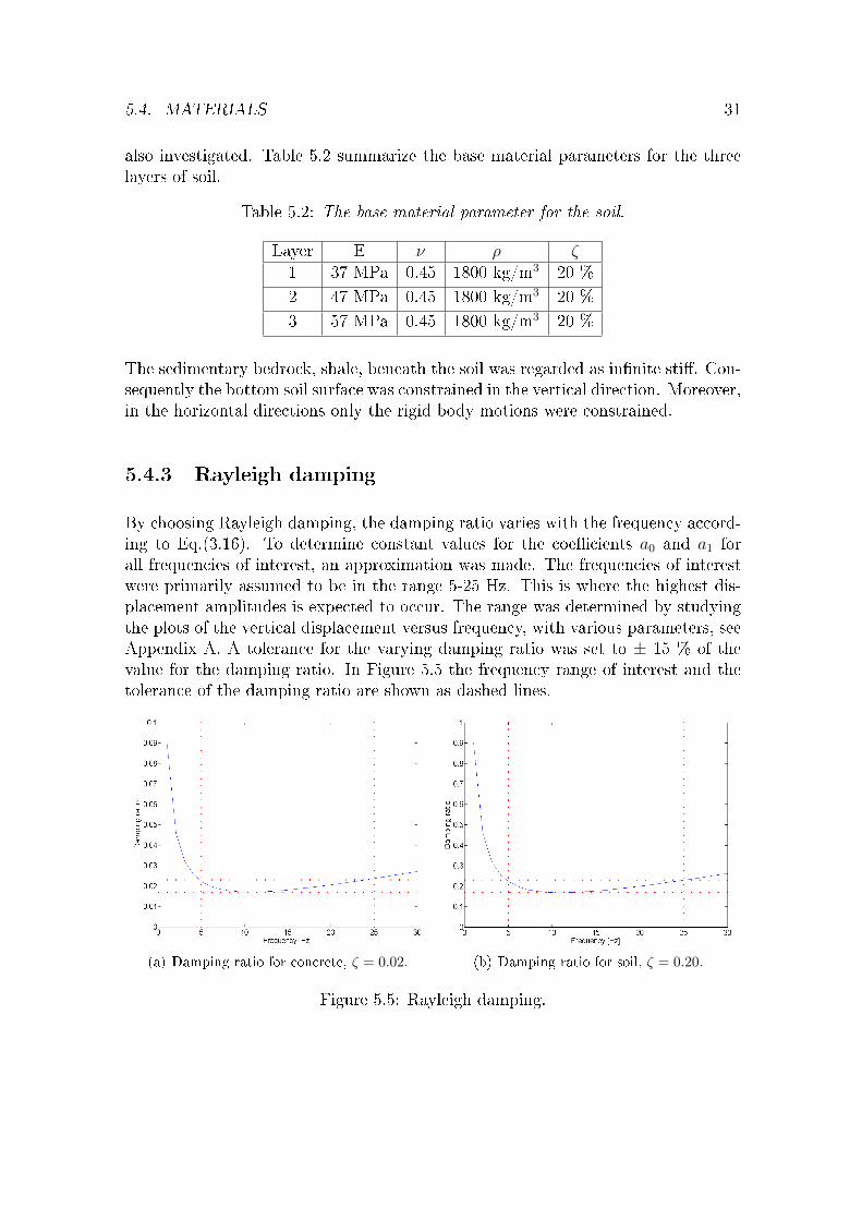
By choosing Rayleigh damping, the damping ratio varies with the frequency accord-ing to Eq.(3.16). To determine constant values for the coe�cients a0 and a1 forall frequencies of interest, an approximation was made. The frequencies of interestwere primarily assumed to be in the range 5-25 Hz. This is where the highest dis-placement amplitudes is expected to occur. The range was determined by studyingthe plots of the vertical displacement versus frequency, with various parameters, seeAppendix A. A tolerance for the varying damping ratio was set to ± 15 % of thevalue for the damping ratio. In Figure 5.5 the frequency range of interest and thetolerance of the damping ratio are shown as dashed lines.
(a) Damping ratio for concrete, ζ = 0.02. (b) Damping ratio for soil, ζ = 0.20.
Figure 5.5: Rayleigh damping.
32 5. FE MODEL
By choosing a certain damping ratio the damping ratio versus frequency may beplotted. Figures in Figure 5.5 show plots of the damping ratio versus frequency forthe base values for both concrete and soil.
5.5 Loading
The structure was analysed for two types of dynamic loads. In the Harmonic loadingchapter sinusoidal harmonic concentrated loading was applied and in the Transientloading chapter transient walking loads was applied.
6
Modelling Results
6.1 Evaluation points
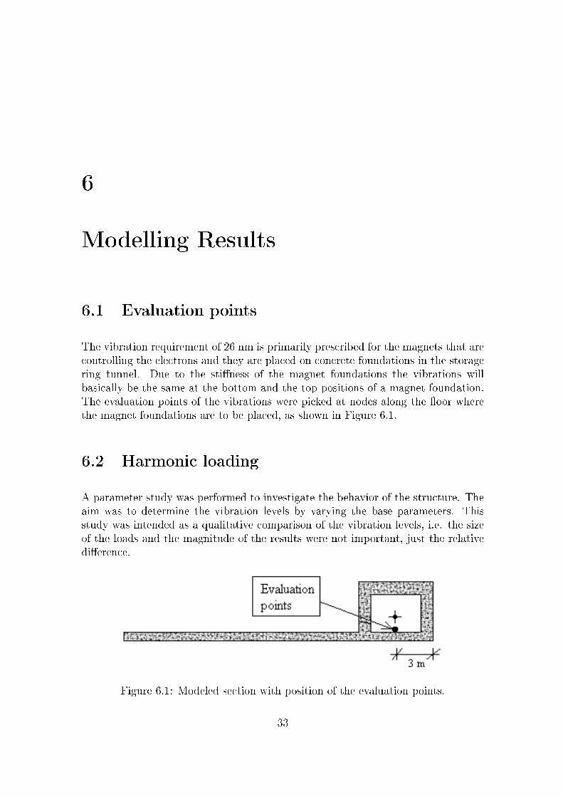
The vibration requirement of 26 nm is primarily prescribed for the magnets that arecontrolling the electrons and they are placed on concrete foundations in the storagering tunnel. Due to the sti�ness of the magnet foundations the vibrations willbasically be the same at the bottom and the top positions of a magnet foundation.The evaluation points of the vibrations were picked at nodes along the �oor wherethe magnet foundations are to be placed, as shown in Figure 6.1.
6.2 Harmonic loading
A parameter study was performed to investigate the behavior of the structure. Theaim was to determine the vibration levels by varying the base parameters. Thisstudy was intended as a qualitative comparison of the vibration levels, i.e. the sizeof the loads and the magnitude of the results were not important, just the relativedi�erence.
Figure 6.1: Modeled section with position of the evaluation points.
33
34 6. MODELLING RESULTS
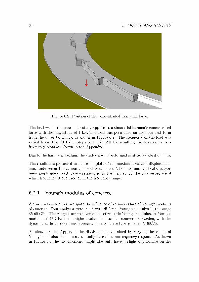
Figure 6.2: Position of the concentrated harmonic force.
The load was in the parameter study applied as a sinusoidal harmonic concentratedforce with the magnitude of 1 kN. The load was positioned on the �oor and 10 mfrom the outer boundary, as shown in Figure 6.2. The frequency of the load wasvaried from 0 to 40 Hz in steps of 1 Hz. All the resulting displacement versusfrequency plots are shown in the Appendix.
Due to the harmonic loading, the analyses were performed in steady-state dynamics.
The results are presented in �gures as plots of the maximum vertical displacementamplitude versus the various choice of parameters. The maximum vertical displace-ment amplitude of each case was sampled at the magnet foundation irrespective ofwhich frequency it occurred at in the frequency range.
6.2.1 Young's modulus of concrete
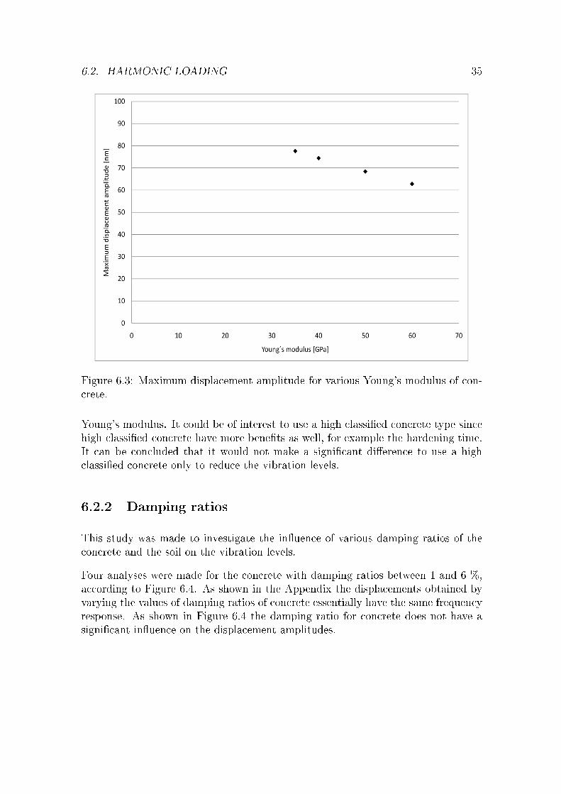
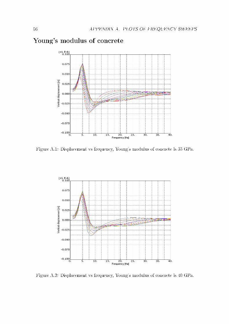
A study was made to investigate the in�uence of various values of Young's modulusof concrete. Four analyses were made with di�erent Young's modulus in the range35-60 GPa. The range is set to cover values of realistic Young's modulus. A Young'smodulus of 47 GPa is the highest value for classi�ed concrete in Sweden, with thedynamic addition taken into account. This concrete type is called C 60/75.
As shown in the Appendix the displacements obtained by varying the values ofYoung's modulus of concrete essentially have the same frequency response. As shownin Figure 6.3 the displacement amplitudes only have a slight dependence on the
6.2. HARMONIC LOADING 35
Figure 6.3: Maximum displacement amplitude for various Young's modulus of con-crete.
Young's modulus. It could be of interest to use a high classi�ed concrete type sincehigh classi�ed concrete have more bene�ts as well, for example the hardening time.It can be concluded that it would not make a signi�cant di�erence to use a highclassi�ed concrete only to reduce the vibration levels.
6.2.2 Damping ratios
This study was made to investigate the in�uence of various damping ratios of theconcrete and the soil on the vibration levels.
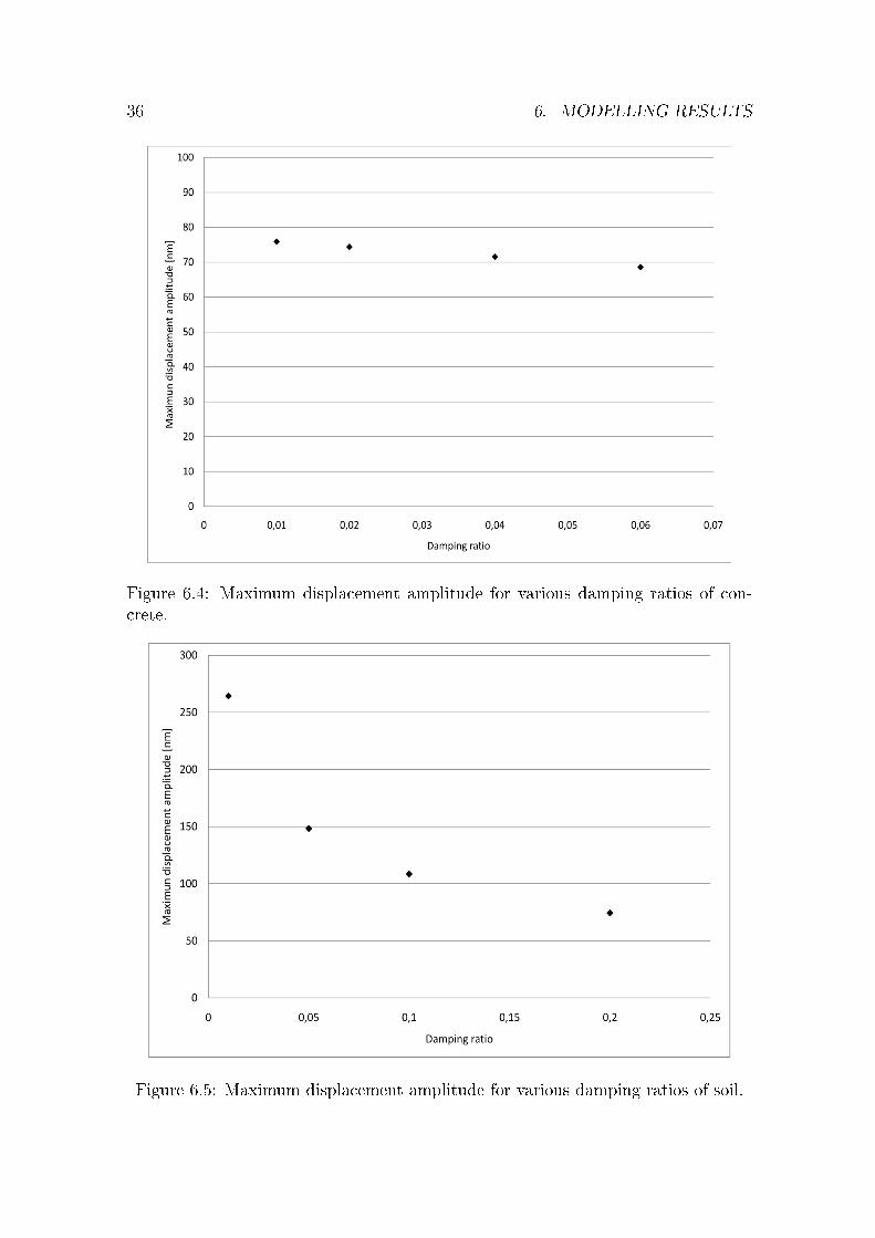
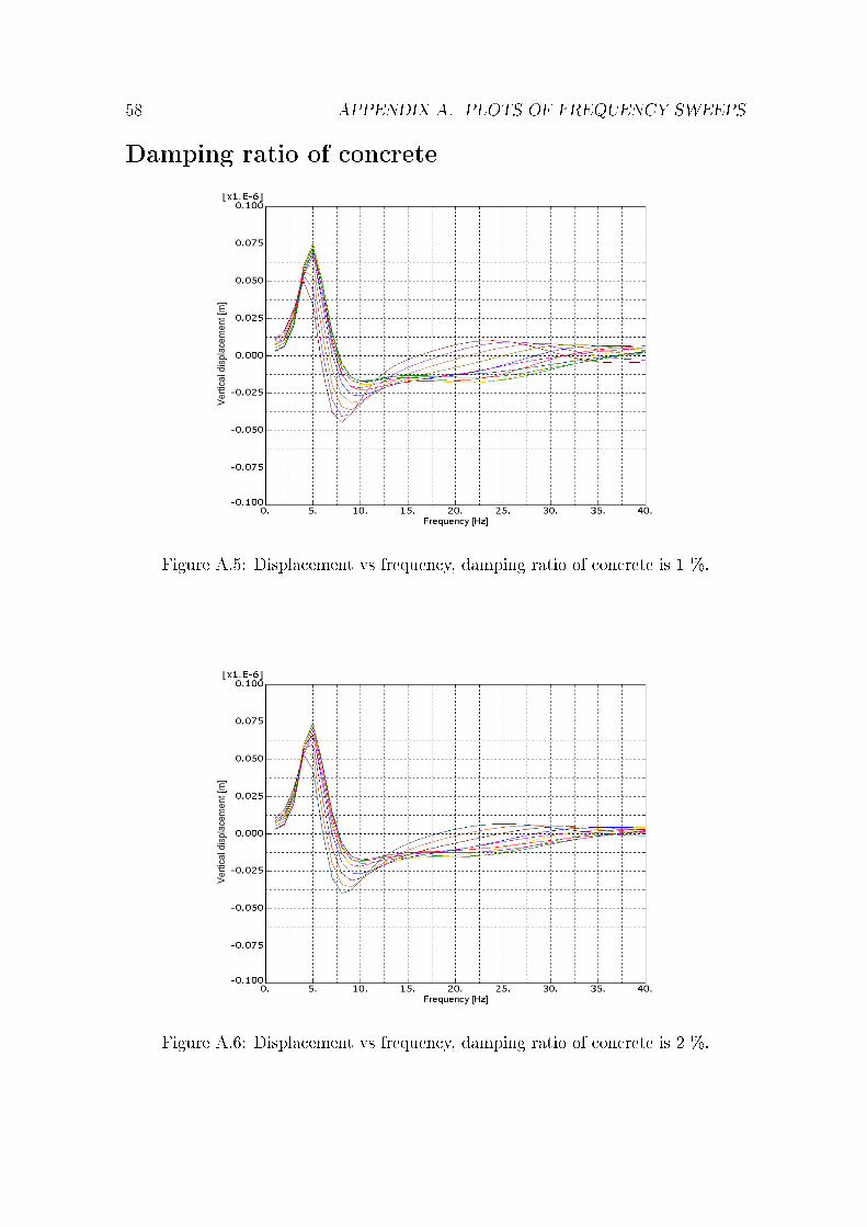
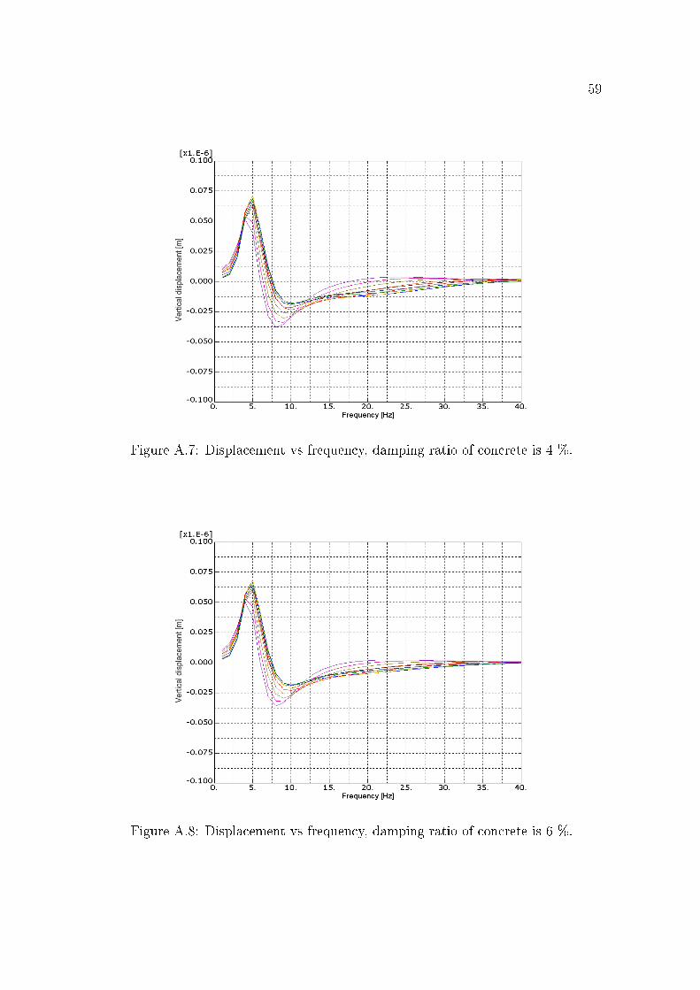
Four analyses were made for the concrete with damping ratios between 1 and 6 %,according to Figure 6.4. As shown in the Appendix the displacements obtained byvarying the values of damping ratios of concrete essentially have the same frequencyresponse. As shown in Figure 6.4 the damping ratio for concrete does not have asigni�cant in�uence on the displacement amplitudes.
36 6. MODELLING RESULTS
Figure 6.4: Maximum displacement amplitude for various damping ratios of con-crete.
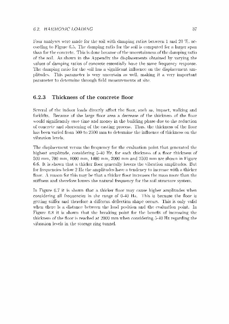
Figure 6.5: Maximum displacement amplitude for various damping ratios of soil.
6.2. HARMONIC LOADING 37
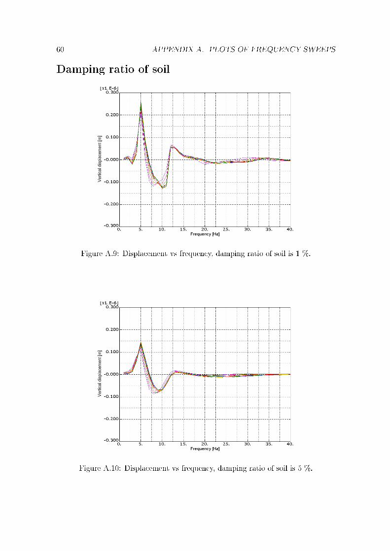
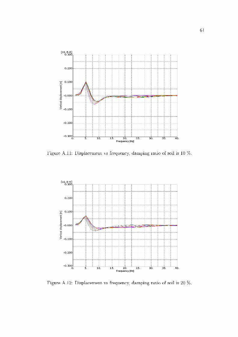
Four analyses were made for the soil with damping ratios between 1 and 20 %, ac-cording to Figure 6.5. The damping ratio for the soil is computed for a larger spanthan for the concrete. This is done because of the uncertainness of the damping ratioof the soil. As shown in the Appendix the displacements obtained by varying thevalues of damping ratios of concrete essentially have the same frequency response.The damping ratio for the soil has a signi�cant in�uence on the displacement am-plitudes. This parameter is very uncertain as well, making it a very importantparameter to determine through �eld measurements at site.
6.2.3 Thickness of the concrete �oor
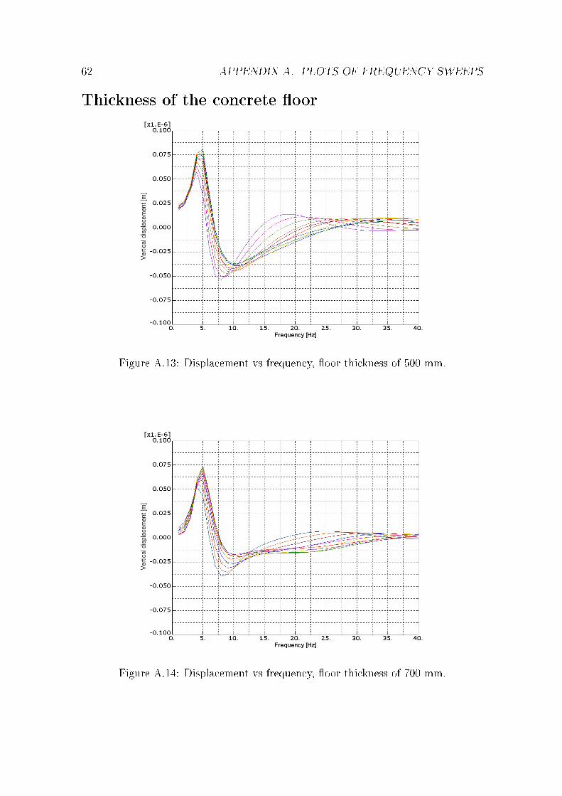
Several of the indoor loads directly a�ect the �oor, such as, impact, walking andforklifts. Because of the large �oor area a decrease of the thickness of the �oorwould signi�cantly save time and money in the building phase due to the reductionof concrete and shortening of the casting process. Thus, the thickness of the �oorhas been varied from 500 to 2500 mm to determine the in�uence of thickness on thevibration levels.
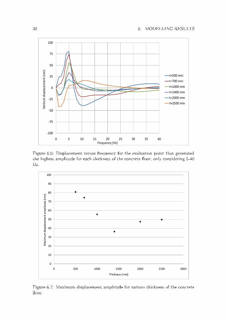
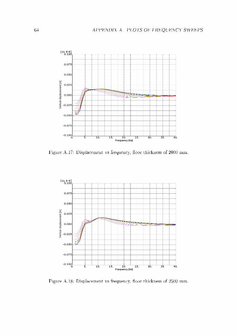
The displacement versus the frequency for the evaluation point that generated thehighest amplitude, considering 5-40 Hz, for each thickness of a �oor thickness of500 mm, 700 mm, 1000 mm, 1400 mm, 2000 mm and 2500 mm are shown in Figure6.6. It is shown that a thicker �oor generally lowers the vibration amplitudes. Butfor frequencies below 2 Hz the amplitudes have a tendency to increase with a thicker�oor. A reason for this may be that a thicker �oor increases the mass more than thesti�ness and therefore lowers the natural frequency for the soil-structure system.
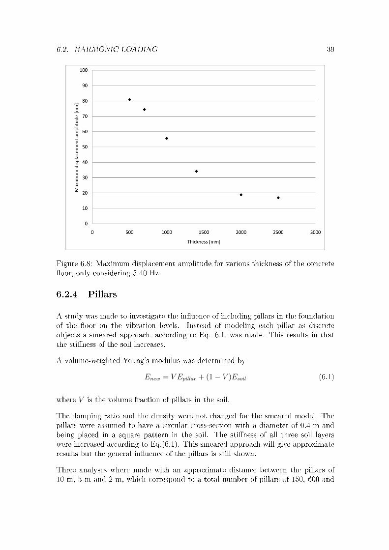
In Figure 6.7 it is shown that a thicker �oor may cause higher amplitudes whenconsidering all frequencies in the range of 0-40 Hz. This is because the �oor isgetting sti�er and therefore a di�erent de�ection shape occurs. This is only validwhen there is a distance between the load position and the evaluation point. InFigure 6.8 it is shown that the breaking point for the bene�t of increasing thethickness of the �oor is reached at 2000 mm when considering 5-40 Hz regarding thevibration levels in the storage ring tunnel.
38 6. MODELLING RESULTS
Figure 6.6: Displacement versus frequency for the evaluation point that generatedthe highest amplitude for each thickness of the concrete �oor, only considering 5-40Hz.
Figure 6.7: Maximum displacement amplitude for various thickness of the concrete�oor.
6.2. HARMONIC LOADING 39
Figure 6.8: Maximum displacement amplitude for various thickness of the concrete�oor, only considering 5-40 Hz.
6.2.4 Pillars
A study was made to investigate the in�uence of including pillars in the foundationof the �oor on the vibration levels. Instead of modeling each pillar as discreteobjects a smeared approach, according to Eq. 6.1, was made. This results in thatthe sti�ness of the soil increases.
A volume-weighted Young's modulus was determined by
Enew = V Epillar + (1− V )Esoil (6.1)
where V is the volume fraction of pillars in the soil.
The damping ratio and the density were not changed for the smeared model. Thepillars were assumed to have a circular cross-section with a diameter of 0.4 m andbeing placed in a square pattern in the soil. The sti�ness of all three soil layerswere increased according to Eq.(6.1). This smeared approach will give approximateresults but the general in�uence of the pillars is still shown.
Three analyses where made with an approximate distance between the pillars of10 m, 5 m and 2 m, which correspond to a total number of pillars of 150, 600 and
40 6. MODELLING RESULTS
3500 pillars.
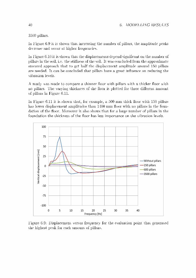
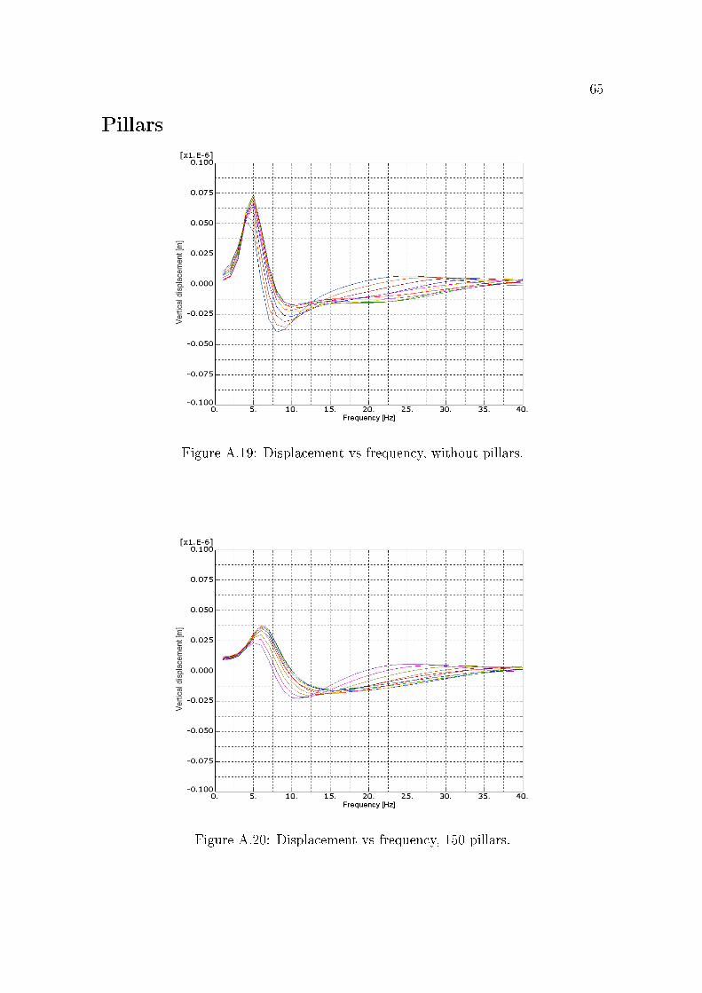
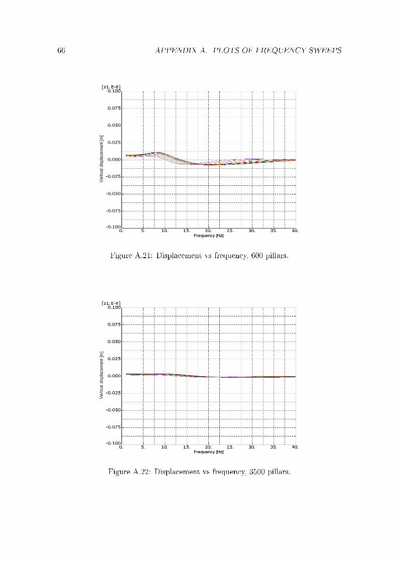
In Figure 6.9 it is shown that increasing the number of pillars, the amplitude peaksdecrease and occur at higher frequencies.
In Figure 6.10 it is shown that the displacements depend signi�cant on the number ofpillars in the soil, i.e. the sti�ness of the soil. It was concluded from the approximatesmeared approach that to get half the displacement amplitude around 150 pillarsare needed. It can be concluded that pillars have a great in�uence on reducing thevibration levels.
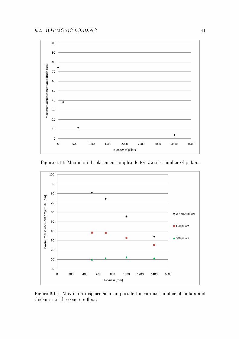
A study was made to compare a thinner �oor with pillars with a thicker �oor withno pillars. The varying thickness of the �oor is plotted for three di�erent amountof pillars in Figure 6.11.
In Figure 6.11 it is shown that, for example, a 500 mm thick �oor with 150 pillarshas lower displacement amplitudes than 1400 mm �oor with no pillars in the foun-dation of the �oor. Moreover it also shows that for a large number of pillars in thefoundation the thickness of the �oor has less importance on the vibration levels.
Figure 6.9: Displacement versus frequency for the evaluation point that generatedthe highest peak for each amount of pillars.
6.2. HARMONIC LOADING 41
Figure 6.10: Maximum displacement amplitude for various number of pillars.
Figure 6.11: Maximum displacement amplitude for various number of pillars andthickness of the concrete �oor.
42 6. MODELLING RESULTS
6.2.5 Divided �oor
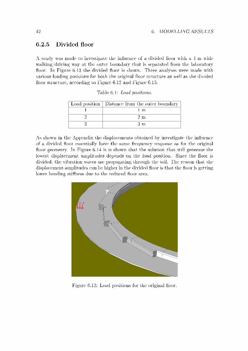
A study was made to investigate the in�uence of a divided �oor with a 4 m widewalking/driving way at the outer boundary that is separated from the laboratory�oor. In Figure 6.13 the divided �oor is shown. Three analyses were made withvarious loading positions for both the original �oor structure as well as the divided�oor structure, according to Figure 6.12 and Figure 6.13.
Table 6.1: Load positions.
Load position Distance from the outer boundary1 1 m
2 2 m
3 3 m
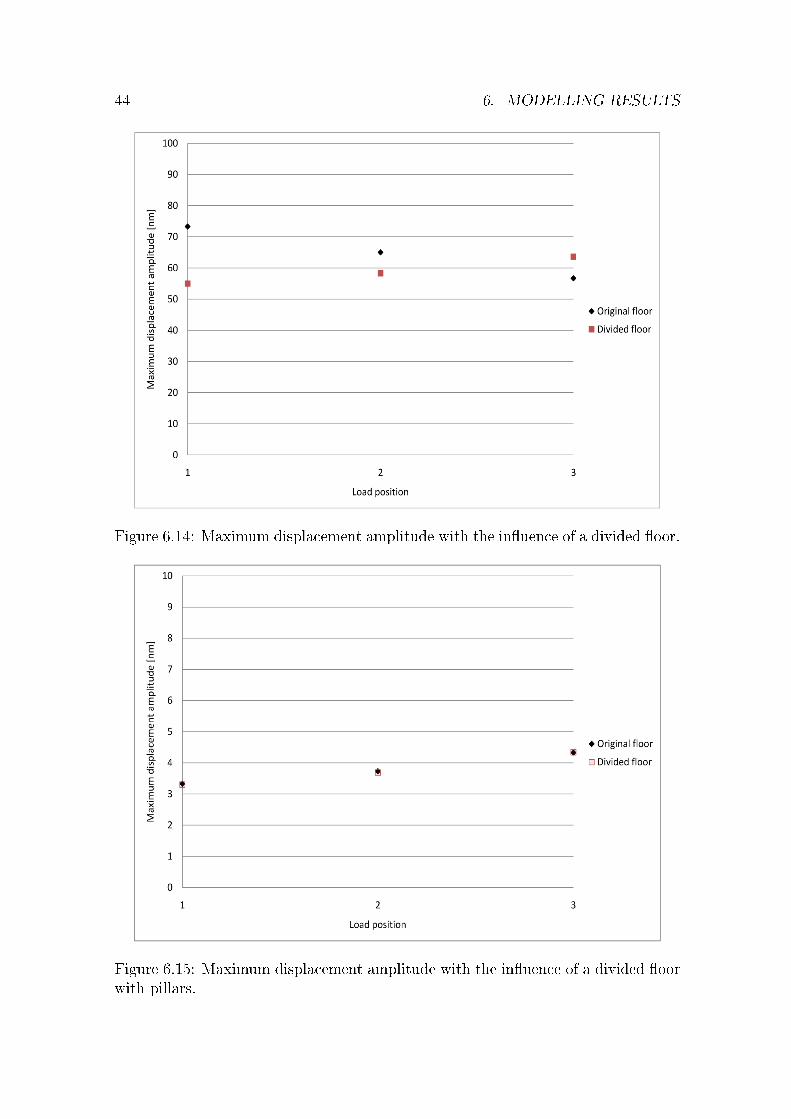
As shown in the Appendix the displacements obtained by investigate the in�uenceof a divided �oor essentially have the same frequency response as for the original�oor geometry. In Figure 6.14 it is shown that the solution that will generate thelowest displacement amplitudes depends on the load position. Since the �oor isdivided, the vibration waves are propagating through the soil. The reason that thedisplacement amplitudes can be higher in the divided �oor is that the �oor is gettinglower bending sti�ness due to the reduced �oor area.
Figure 6.12: Load positions for the original �oor.
6.2. HARMONIC LOADING 43
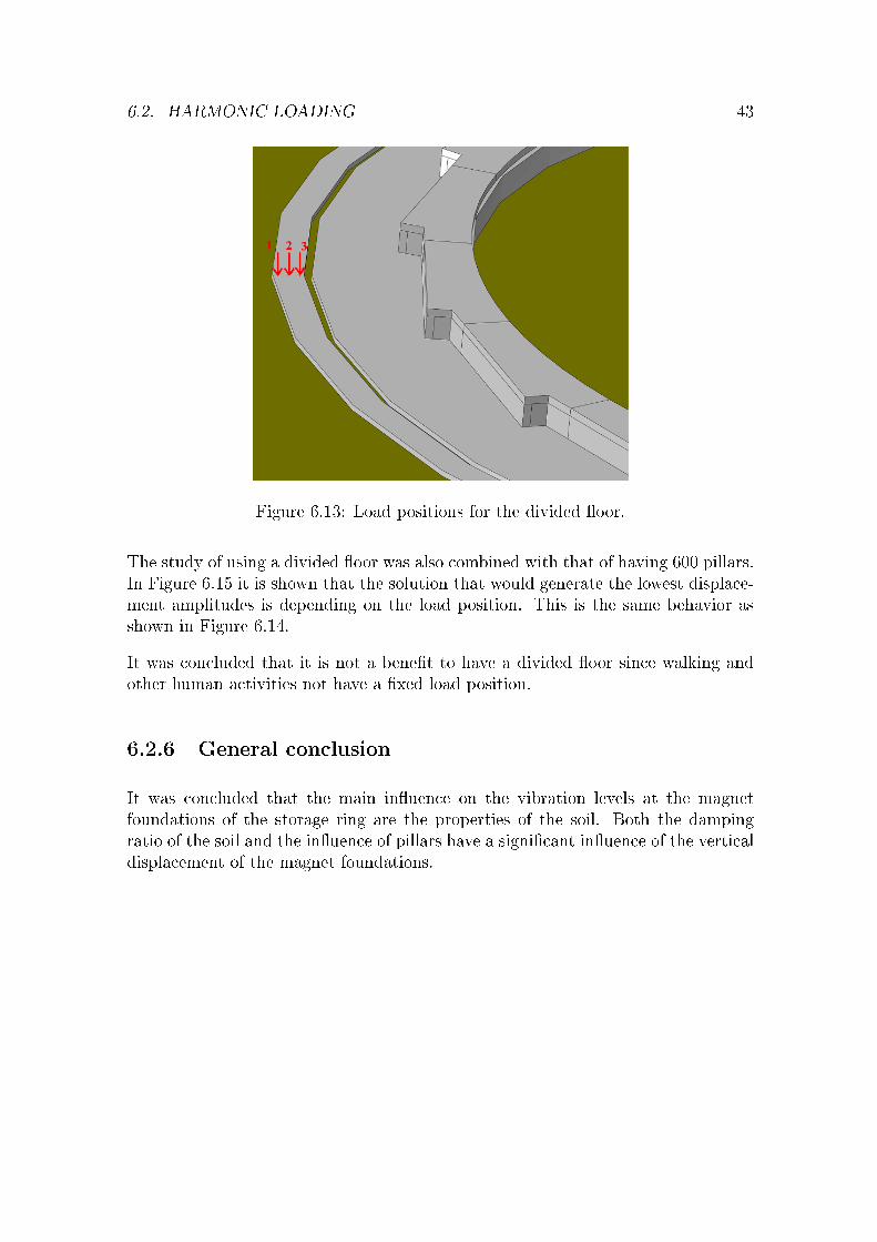
Figure 6.13: Load positions for the divided �oor.
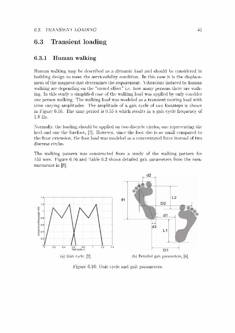
The study of using a divided �oor was also combined with that of having 600 pillars.In Figure 6.15 it is shown that the solution that would generate the lowest displace-ment amplitudes is depending on the load position. This is the same behavior asshown in Figure 6.14.
It was concluded that it is not a bene�t to have a divided �oor since walking andother human activities not have a �xed load position.
6.2.6 General conclusion
It was concluded that the main in�uence on the vibration levels at the magnetfoundations of the storage ring are the properties of the soil. Both the dampingratio of the soil and the in�uence of pillars have a signi�cant in�uence of the verticaldisplacement of the magnet foundations.
44 6. MODELLING RESULTS
Figure 6.14: Maximum displacement amplitude with the in�uence of a divided �oor.
Figure 6.15: Maximum displacement amplitude with the in�uence of a divided �oorwith pillars.
6.3. TRANSIENT LOADING 45
6.3 Transient loading
6.3.1 Human walking
Human walking may be described as a dynamic load and should be considered inbuilding design to meet the serviceability condition. In this case it is the displace-ment of the magnets that determines the requirement. Vibrations induced by humanwalking are depending on the "crowd e�ect" i.e. how many persons there are walk-ing. In this study a simpli�ed case of the walking load was applied by only considerone person walking. The walking load was modeled as a transient moving load withtime varying amplitudes. The amplitude of a gait cycle of two footsteps is shownin Figure 6.16. The time period is 0.55 s which results in a gait cycle frequency of1.8 Hz.
Normally, the loading should be applied on two discrete circles, one representing theheel and one the forefoot, [7]. However, since the foot size is so small compared tothe �oor extension, the foot load was modeled as a concentrated force instead of twodiscrete circles.
The walking pattern was constructed from a study of the walking pattern for150 men. Figure 6.16 and Table 6.2 shows detailed gait parameters from the mea-surements in [8].
(a) Gait cycle, [7]. (b) Detailed gait parameters, [8].
Figure 6.16: Gait cycle and gait parameters.
46 6. MODELLING RESULTS
Only the parameters L1 and L2 in Table 6.2 was considered here since the loading wasapplied on a straight line, because of the �oor extension. The lengthwise distancewas set to 65 cm according to Table 6.2.
Table 6.2: Detailed gait parameters, [8].
Parameter Value [cm]l1 26.5L1 65L2 65d1 5d2 5d3 2.2D1 10D2 19
6.3.2 Walking load
To simulate the walking load as realistic as possible, it was applied as a transientmoving load. Analyses were made for two load patterns on the concrete �oor cor-responding to tangential and radial walking patterns. The duration of the analysesof the walking patterns was 7 s.
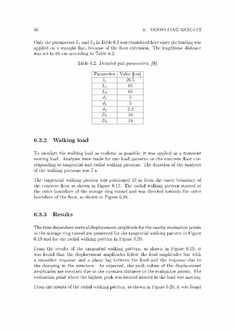
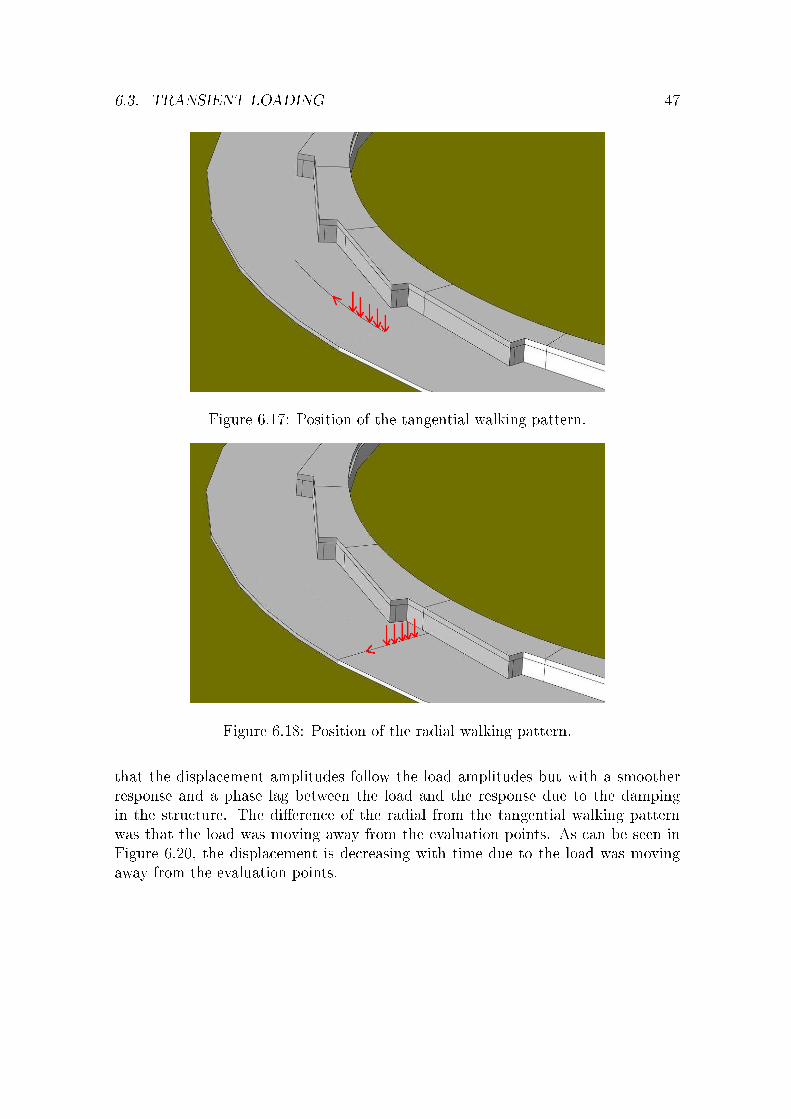
The tangential walking pattern was positioned 10 m from the outer boundary ofthe concrete �oor as shown in Figure 6.17. The radial walking pattern started atthe outer boundary of the storage ring tunnel and was directed towards the outerboundary of the �oor, as shown in Figure 6.18.
6.3.3 Results
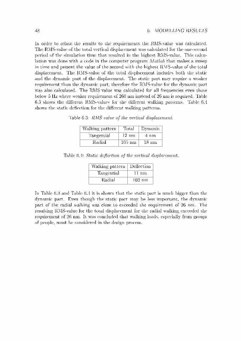
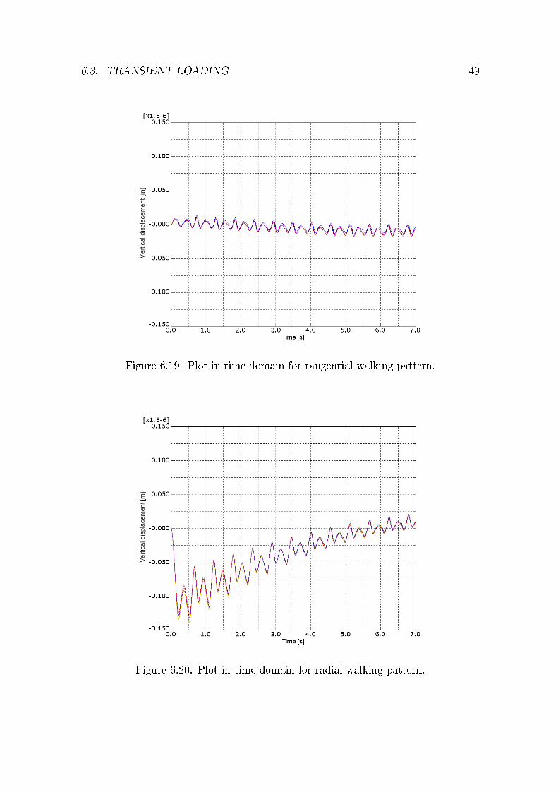
The time dependent vertical displacement amplitude for the nearby evaluation pointsin the storage ring tunnel are presented for the tangential walking pattern in Figure6.19 and for the radial walking pattern in Figure 6.20.
From the results of the tangential walking pattern, as shown in Figure 6.19, itwas found that the displacement amplitudes follow the load amplitudes but witha smoother response and a phase lag between the load and the response due tothe damping in the structure. As expected, the peak values of the displacementamplitudes are constant due to the constant distance to the evaluation points. Theevaluation point where the highest peak was located altered as the load was moving.
From the results of the radial walking pattern, as shown in Figure 6.20, it was found
6.3. TRANSIENT LOADING 47
Figure 6.17: Position of the tangential walking pattern.
Figure 6.18: Position of the radial walking pattern.
that the displacement amplitudes follow the load amplitudes but with a smootherresponse and a phase lag between the load and the response due to the dampingin the structure. The di�erence of the radial from the tangential walking patternwas that the load was moving away from the evaluation points. As can be seen inFigure 6.20, the displacement is decreasing with time due to the load was movingaway from the evaluation points.
48 6. MODELLING RESULTS
In order to relate the results to the requirements the RMS-value was calculated.The RMS-value of the total vertical displacement was calculated for the one-secondperiod of the simulation time that resulted in the highest RMS-value. This calcu-lation was done with a code in the computer program Matlab that makes a sweepin time and present the value of the second with the highest RMS-value of the totaldisplacement. The RMS-value of the total displacement includes both the staticand the dynamic part of the displacement. The static part may require a weakerrequirement than the dynamic part, therefore the RMS-value for the dynamic partwas also calculated. The RMS-value was calculated for all frequencies even thosebelow 5 Hz where weaker requirement of 260 nm instead of 26 nm is required. Table6.3 shows the di�erent RMS-values for the di�erent walking patterns. Table 6.4shows the static de�ection for the di�erent walking patterns.
Table 6.3: RMS-value of the vertical displacement.
Walking pattern Total Dynamic
Tangential 12 nm 4 nm
Radial 105 nm 18 nm
Table 6.4: Static de�ection of the vertical displacement.
Walking pattern De�ection
Tangential 11 nm
Radial 103 nm
In Table 6.3 and Table 6.4 it is shown that the static part is much bigger than thedynamic part. Even though the static part may be less important, the dynamicpart of the radial walking was close to exceeded the requirement of 26 nm. Theresulting RMS-value for the total displacement for the radial walking exceeded therequirement of 26 nm. It was concluded that walking loads, especially from groupsof people, must be considered in the design process.
6.3. TRANSIENT LOADING 49
Figure 6.19: Plot in time domain for tangential walking pattern.
Figure 6.20: Plot in time domain for radial walking pattern.

Denna sida skall vara tom!
7
Discussion and Suggestions for
Further Work
It was discovered from the parameter study that the material parameters of the soilgreatly in�uences the vibration levels of the �oor. Since there is a lack of knowledgeregarding the material parameters for the soil there is a need for determining those.There are especially two parameters for the soil that control the soil and thus thestructure; the Young's modulus and the damping ratio. The Young's modulus isgiven in the geotechnical report but it should not be used for detailed design. For thebedrock there is no information about material parameters. The material parametersare needed to get a reliable output that can be compared with the requirements.
The smeared approach that was used to determine the equivalent sti�ness of thesoil when considering the pillars was an approximation. How good the results fromthis approximation are depending on several things like the bending wave lengthand the position of the pillars. To get more reliable results discrete pillars would beintroduced discrete pillars in the model.
In the parameter study, the harmonic load was only applied at one location. Theloading position should be varied because the relation between the thickness of the�oor and the displacement of the evaluation points depends of the distance betweenthe load position and the evaluation point.
To ensure that the strict requirements are ful�lled, more realistic loads must beconsidered. Such loads are for instance working machines, tra�c from inside thebuilding such as forklifts and outside such as tra�c from nearby roads. Also agroup of people walking must be considered. A FFT should also be done for thedisplacements in the time domain to see the frequency content of the walking load.It may be shown in the frequency domain that some peaks are below 5 Hz and maytherefore be excluded from the calculations of the RMS-value.
51

52 7. DISCUSSION AND SUGGESTIONS FOR FURTHER WORK
If the tra�c load from the nearby highway are to be analysed the Linac and thestorage ring must be considered in the same model since the Linac could work as abarrier for the vibrations from the tra�c due to its position between the ring andthe highway.
Besides from the opportunities given in the parameter study dampers can be usedas a solution to reduce the vibration levels. For one example the in�uence of rubbermats could be investigated.
Bibliography
[1] Boverket (2004). Boverkets handbok om betongkonstruktioner, BBK 04. Bover-ket
[2] Ottosen N. S. and Petersson H. (1992). Introduction to the �nite elementmethod. Prentice Hall
[3] Anil K. Chopra (1995). Dynamics of structures. Prentice Hall
[4] Engström Björn (2004). Beräkning av betongkonstruktioner. Institutionen förkonstruktion och mekanik, Chalmers tekniska högskola.
[5] Axelsson Kennet (2005). Introduktion till GEOTEKNIKEN. Instutitionen förGeovetenskaper, Uppsala Universitet.
[6] Sällfors Göran (2008). Kurspärm GRUNDLÄGGNINGSTEKNIK. Instutionenför Byggvetenskaper, Lunds Universitet.
[7] Bard Delphine, Persson Kent & Sandberg Göran (2008). Human footsteps in-duced �oor vibration. Acoustics'08, Paris France, July 2008.
[8] Claesson Jimmy (2008). Simulering av stomljud med hjälp av gångmönster-statistik Division of Engineering Acoustics, Lunds Tekniska Högskola, ReportTVBA 5038.
[9] SIMULA (2008). Abaqus manual 6.9
[10] Heyden Susanne, Dahlblom Ola, Olsson Anders & Sandberg Göran. (2007).Indroduktion till Strukturmekaniken KFS i Lund AB
[11] MAX-lab, Lunds Universitet. (2009). MAX-lab - MAX IV
[12] SWECO AB. (2009). Drawings MAX IV
[13] Ohlrich M, Hugin C.T. (2003). On the in�uence of boundary constraints andangled ba�e arrangements on sound radiation from rectangular plates Journalof Sound and Vibration 277, 2004.
53

54 BIBLIOGRAPHY
[14] SWECO AB. (2009). MAX IV, LUND. ÖVERSIKTLIG GEOTEKNISKUTREDNING (TPgeo).
Appendix A
Plots of frequency sweeps
Plots of frequency sweeps for varying parameters according to the parameter studyin Modelling Results.
55
56 APPENDIX A. PLOTS OF FREQUENCY SWEEPS
Young's modulus of concrete
Figure A.1: Displacement vs frequency, Young's modulus of concrete is 35 GPa.
Figure A.2: Displacement vs frequency, Young's modulus of concrete is 40 GPa.

57
Figure A.3: Displacement vs frequency, Young's modulus of concrete is 50 GPa.
Figure A.4: Displacement vs frequency, Young's modulus of concrete is 60 GPa.
58 APPENDIX A. PLOTS OF FREQUENCY SWEEPS
Damping ratio of concrete
Figure A.5: Displacement vs frequency, damping ratio of concrete is 1 %.
Figure A.6: Displacement vs frequency, damping ratio of concrete is 2 %.
59
Figure A.7: Displacement vs frequency, damping ratio of concrete is 4 %.
Figure A.8: Displacement vs frequency, damping ratio of concrete is 6 %.
60 APPENDIX A. PLOTS OF FREQUENCY SWEEPS
Damping ratio of soil
Figure A.9: Displacement vs frequency, damping ratio of soil is 1 %.
Figure A.10: Displacement vs frequency, damping ratio of soil is 5 %.
61
Figure A.11: Displacement vs frequency, damping ratio of soil is 10 %.
Figure A.12: Displacement vs frequency, damping ratio of soil is 20 %.
62 APPENDIX A. PLOTS OF FREQUENCY SWEEPS
Thickness of the concrete �oor
Figure A.13: Displacement vs frequency, �oor thickness of 500 mm.
Figure A.14: Displacement vs frequency, �oor thickness of 700 mm.

63
Figure A.15: Displacement vs frequency, �oor thickness of 1000 mm.
Figure A.16: Displacement vs frequency, �oor thickness of 1400 mm.
64 APPENDIX A. PLOTS OF FREQUENCY SWEEPS
Figure A.17: Displacement vs frequency, �oor thickness of 2000 mm.
Figure A.18: Displacement vs frequency, �oor thickness of 2500 mm.
65
Pillars
Figure A.19: Displacement vs frequency, without pillars.
Figure A.20: Displacement vs frequency, 150 pillars.
66 APPENDIX A. PLOTS OF FREQUENCY SWEEPS
Figure A.21: Displacement vs frequency, 600 pillars.
Figure A.22: Displacement vs frequency, 3500 pillars.
67
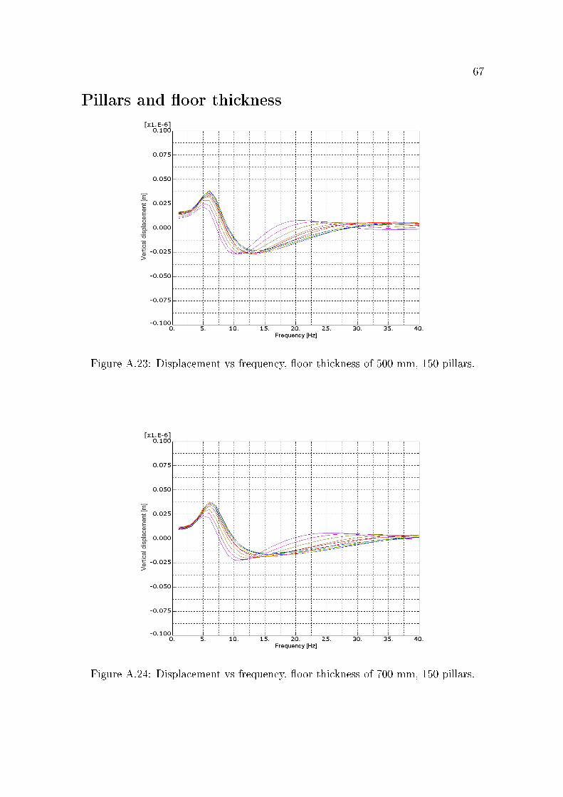
Pillars and �oor thickness
Figure A.23: Displacement vs frequency, �oor thickness of 500 mm, 150 pillars.
Figure A.24: Displacement vs frequency, �oor thickness of 700 mm, 150 pillars.
68 APPENDIX A. PLOTS OF FREQUENCY SWEEPS
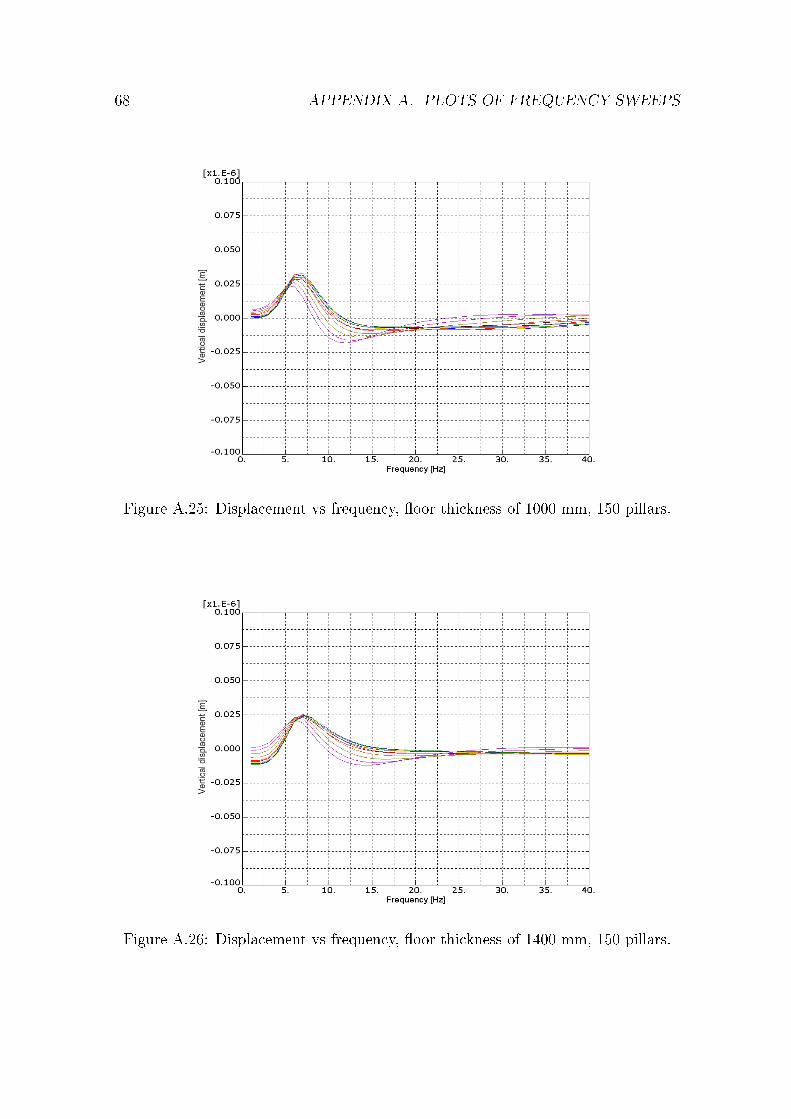
Figure A.25: Displacement vs frequency, �oor thickness of 1000 mm, 150 pillars.
Figure A.26: Displacement vs frequency, �oor thickness of 1400 mm, 150 pillars.
69
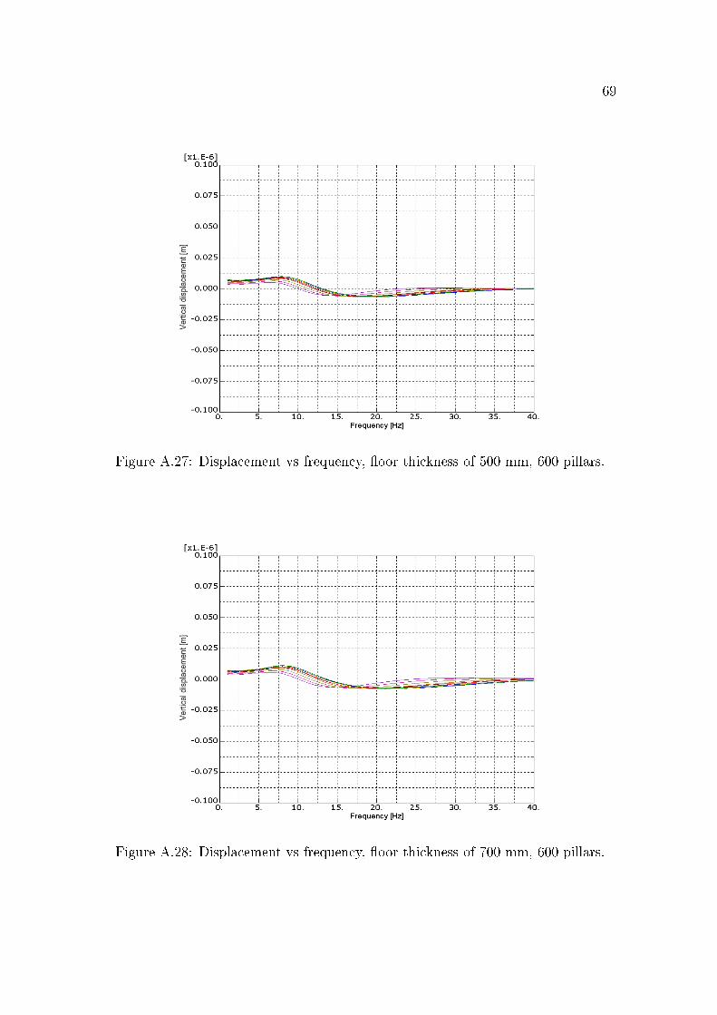
Figure A.27: Displacement vs frequency, �oor thickness of 500 mm, 600 pillars.
Figure A.28: Displacement vs frequency, �oor thickness of 700 mm, 600 pillars.

70 APPENDIX A. PLOTS OF FREQUENCY SWEEPS
Figure A.29: Displacement vs frequency, �oor thickness of 1000 mm, 600 pillars.
Figure A.30: Displacement vs frequency, �oor thickness of 1400 mm, 600 pillars.
71
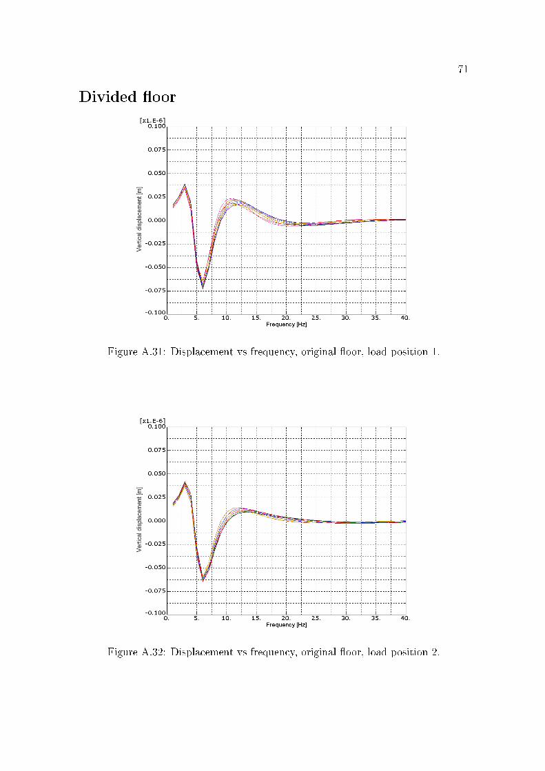
Divided �oor
Figure A.31: Displacement vs frequency, original �oor, load position 1.
Figure A.32: Displacement vs frequency, original �oor, load position 2.
72 APPENDIX A. PLOTS OF FREQUENCY SWEEPS
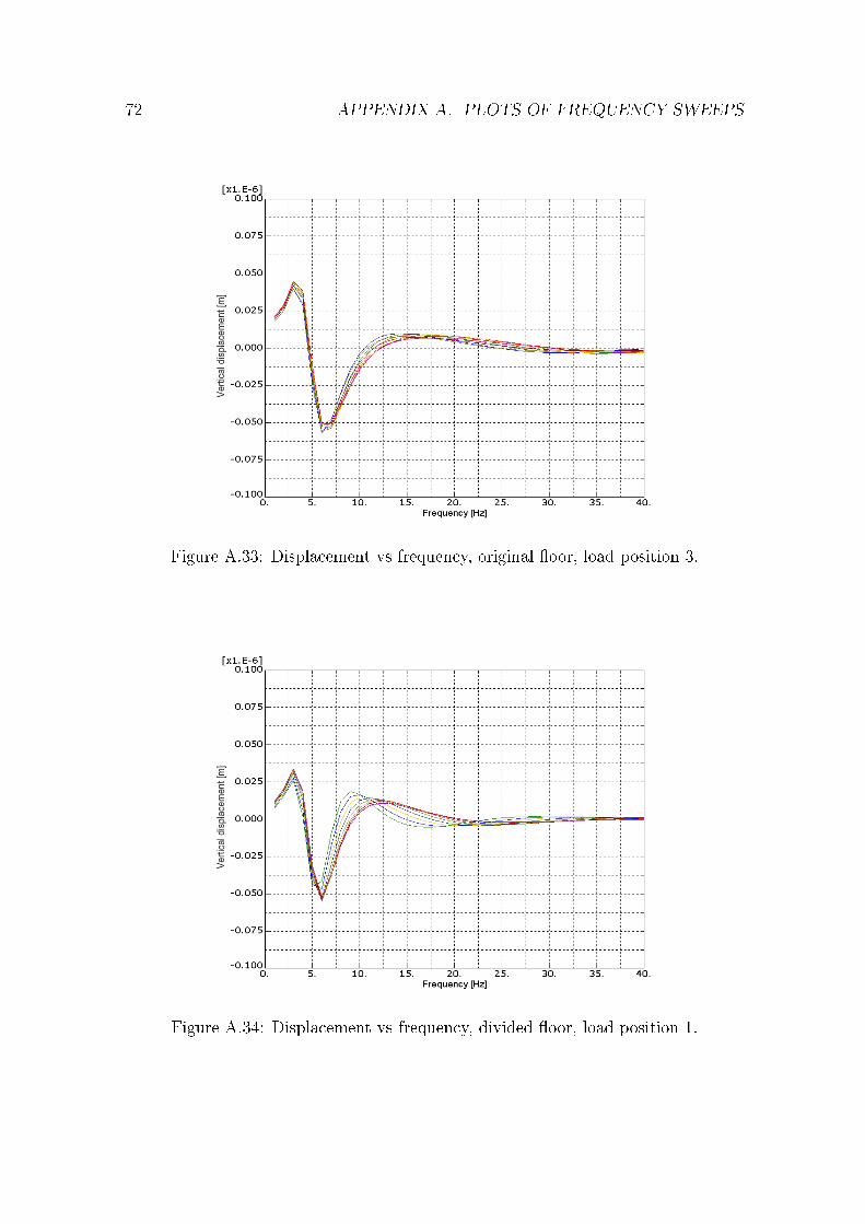
Figure A.33: Displacement vs frequency, original �oor, load position 3.
Figure A.34: Displacement vs frequency, divided �oor, load position 1.
73
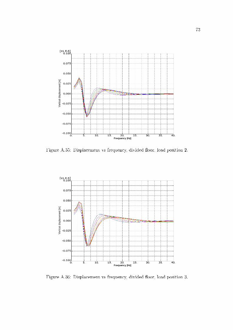
Figure A.35: Displacement vs frequency, divided �oor, load position 2.
Figure A.36: Displacement vs frequency, divided �oor, load position 3.
74 APPENDIX A. PLOTS OF FREQUENCY SWEEPS
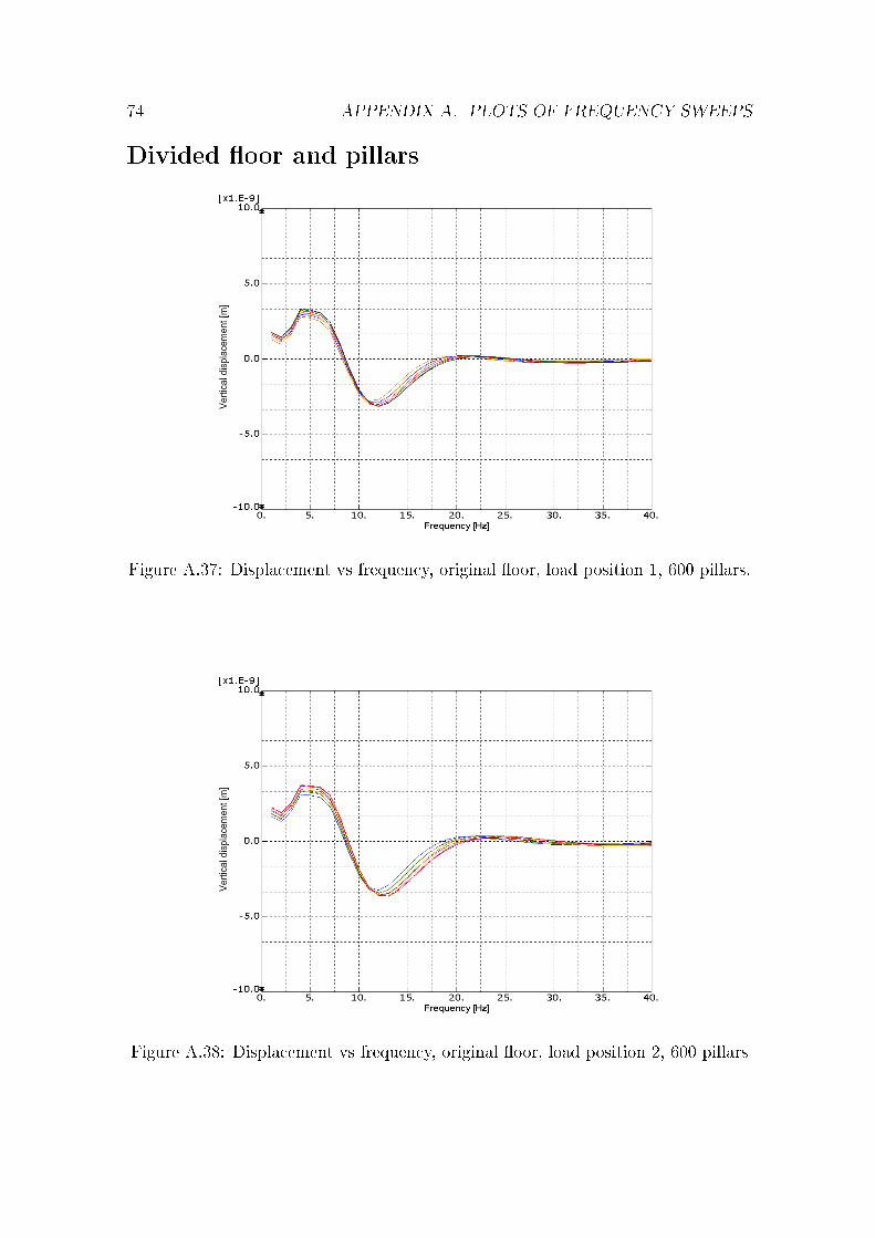
Divided �oor and pillars
Figure A.37: Displacement vs frequency, original �oor, load position 1, 600 pillars.
Figure A.38: Displacement vs frequency, original �oor, load position 2, 600 pillars
75
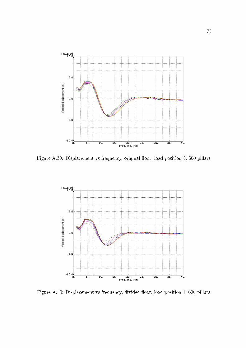
Figure A.39: Displacement vs frequency, original �oor, load position 3, 600 pillars
Figure A.40: Displacement vs frequency, divided �oor, load position 1, 600 pillars
76 APPENDIX A. PLOTS OF FREQUENCY SWEEPS
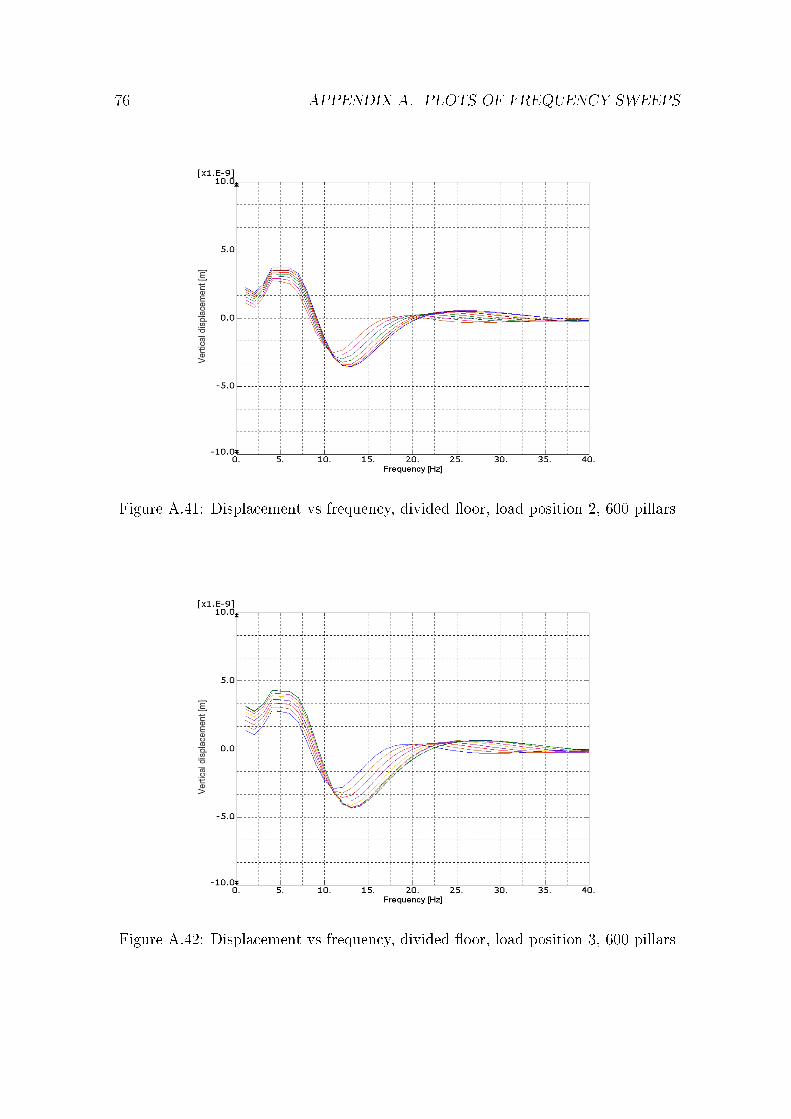
Figure A.41: Displacement vs frequency, divided �oor, load position 2, 600 pillars
Figure A.42: Displacement vs frequency, divided �oor, load position 3, 600 pillars