ANALYSIS OF TRANSIENT, LINEAR WAVE BY THE FINITE DIFFERENCE METHOD · 2017-07-01 · ANALYSIS OF...

LOAN COPY: RETURN TO AFWL (DO-UL)

KIRTLAND AFB, N, M.

ANALYSIS OF TRANSIENT, LINEAR WAVE PROPAGATION IN SHELLS BY THE FINITE DIFFERENCE METHOD

by Thomas L. Geers dad Lawrence H. Sobel

Prepared by

LOCKHEED MISSILES & SPACE COMPANY

Palo Alto, Calif. 74304

for Langley Resenrch Cezzter ,

https://ntrs.nasa.gov/search.jsp?R=19720008223 2020-04-07T00:06:53+00:00Z

TECH LIBRARY KAFB, NM

!

00bZ002 1. R e p a t No. 3. Recipient's C a t a l o g No. 2. Government Accession No.

NASA CR-1885 4. Title and Subtitle 5. Report Date

December 1971 I AHALyGIS OF !llRANSIEiT; WAVE PFlOPAGATIOEI Ill BY 6. PaformiM Ormnization Coda 1 rn F ~ T E DIFFEREHCE- XETEIOD I "

7. Author(s) 8. Performing Organization Report No.

Thomas L. Geers and Lawrence H. Sobel 10. Work Unit No.

Q. Fbrforming Organization Name and Address 134-14-04-01

Gckheed Missiles & Space Company

Palo Alto, Calif. 94304 NAS 1-9111 lockheed Palo Alto Research Lab.

11. Contract or Grant No.

13. Type of Report and Period Covered 12. Sponsoring Agency Name and Address

14. Sponsoring Ag~mcy Code National Aeronautics and Space Administration Contractor Report

. Washington, D.C. 20546 15. Supplementary Notes

16. Abstract

This report contains: (1) analytical and numerical studies pertaining to the limite of applicability of the finite difference method in the solution of transient, linear wave propagation problems i n shells, (2) a recommended computational procedure fo r the use of the method, and (3) a numerical investigation of the response of a cylindrical shell with cutouts t o both longitudinal and radial transient excitations. It i s found that the only inherent limitation of the f in i te difference method i s i t s inabi l i ty to reproduce accurately response discontinuities. This i s not a serious limitation, i n v i e w of natural constraints imposed by the extension of Saint Verant's principle t o wave propagation problems. It i s also found that the short wave length limitations of thin shell (Bernoulli-Euler) theory create significant convergence difficult ies in computed responses to certain types of transverse excitations. These difficult ies may often be overcome, however, through proper selection of finite difference mesh dimensions and temporal or spatial smoothing of the excitation. Finally, it i s found that cutouts produce moderate changes in early- and intermediate time response of a cylindrical. shell t o &symmetric pulse-loads applied a t one end. The cutouts may, however, facil i tate the undesirable late-time transfer of load-injected extensional energy into non-eJdsymmetric flexural response.

17. Key Words (Suggested by Author(s)) 18. Distribution Statement

Wave propagation in shells

Wave propngation by f in i te differences Unclassified - Unlimited

19. Security aaoif. (of this report)

$3 -00 191 Unclassified Unclassified

22. Rice* 21. NO. of P w 20. Security Classif. (of this pge)

~

For =le by the National Technical Information Service, Springfield, Virginio 22151

FOREWORD

The research descr ibed in the p resent repor t was performed under

Contract NAS 1-9111 with the NASA/Langley Research Center, Hampton,

Virginia , wi th D r . J. P . Raney as Contract Monitor. A companion volume,

LMSC LS 69-6, conta ins the resu l t s of a search of t h e l i t e r a t u r e on

l i n e a r t r a n s i e n t wave p ropaga t ion i n e l a s t i c ba r s , p l a t e s and s h e l l s

covering the period 1964 through ear ly 1969.

The authors wish t o thank D r . J . P . Raney, Miss B . J. Durling and

Mr. J. T . Howlett of the NASA/Langley Research Center for providing modal

supe rpos i t i on so lu t ions t o ce r t a in problems invest igated herein. They

a l s o wish t o thank Dr. D . A . Evensen of TRW Systems, Redondo Beach, C a l i f . , for his coopera t ion in coord ina t ing the ana ly t ica l and expe r iwn ta l cu tou t

s tud ies . The au tho r s a l so expres s t he i r app rec i a t ion t o M r . P. S . Jensen of

Lockheed and Mr. Wilson Silsby, recently a t Lockheed bu t now a t t h e J e t

Prbpulsion Laboratories, Pasadena, Calif ., for introducing important modi-

f i c a t i o n s i n t o t h e STAR code . Las t , bu t cer ta in ly no t l eas t , the au thors

e x p r e s s t h e i r g r a t i t u d e t o Mrs. Gloria Sherrard and Miss Jessie Vost i of

Lockheed fo r t he i r pa t i ence and perseverance in the sk i l l fu l p repara t ion

of this r epor t .

iii

TABU aF CONTENTS

Chapter 1. INTRODUCTION

1.1 Response Variables

1.2 Equations of S h e l l Theory

1.3 Various Numerical Methods Solution

1 . 4 The STAR Code: Description and Application

"

"- - Chapter 2. NUMERICAL STUDY OF CONVERGENCE

2.1 Displacement, Velocity and - Acceleration

Response to In-Plane Excitaticm

2.1.1 (2, r) - Exci ta t ions

2.1.2 (z, 3) - Excitat ions

2.1.3 (& 3) - Exci ta t ions

2.1.4 Conclusions

2.2 Displacement, Velocity and Acceleration

Response to Transverse Excitation

2.2.1 (2, r) - Excitat ion

2.2.2 (z, 3) - Exci ta t ion

2.2.3 (& 3) - Excitat ions

2.2.4 Smoothed Exci ta t ions

2.2.5 Conclusions

2.3 Stress/Strain Response - t o In-Plane Excitation

2.3.1 (G, F) -, (Z, F ) -, and

(z, 2) - Exci ta t ions

2.3.2 Conclusions

2.3.3 Comparison with Experimental Data

2 .4 S t ress /S t ra in Response to Transverse Excitation

2.4.1 (z, !E') -, (z, F ) -, and

(& 3) - Exci ta t ions

2.4.2 Smoothed Exci ta t ions 2.4.3 Conclusions

Page 1-1

1-2 1-4 1-7 1-8

Page 2-1

2 -2

2 -2

2 -3 2 :!+

2 -5

2 -6

2 -6 2 -8 2 -8 2 -10

2 -11

2 -12 2 -12

2 -13

2 -13

2 -16 2 -16

2 -17 2 -18

V

ANALYSIS OF TRANSIENT, LINEAR WAVE PROPAGATION

I N SHELLS BY THE FINITE DIFFERENCE METHOD

By Thomas L . Geers and Lawrence H . Sobel Lockheed Missiles & Space Company

Palo Alto, California

Chapter 1

INTRODUCTION

The f i n i t e d i f f e r e n c e method has been used f o r many yea r s i n t he so lu t ion

of d i f fe ren t ia l equa t ions , inc luding those of she l l theory . Because the method

involves the transformation of d i f fe ren t ia l equa t ions for cont inuous var iab les

in to d i f f e rence equa t ions fo r d i sc re t e va r i ab le s , a question of pr imary in te res t

i s the following: A t what mesh s i ze ( i f any ) do the f i n i t e d i f f e rence equa t ions

accurately reproduce the solutions of i n t e r e s t t o t h e d i f f e r e n t i a l e q u a t i o n s ?

This repor t addresses i t se l f to tha t ques t ion as it p e r t a i n s t o t r a n s i e n t ,

l i n e a r wave propagat ion in she l l s .

The motivat ion behind this s tudy was t o provide a suff ic ient ly f i rm under-

standing of t h e t i t l e s u b j e c t t h a t d e t a i l e d comparisons could be made between

t h e f i n i t e d i f f e r e n c e method and other numerical methods of ana lys i s . A s the

study progressed, it became p o s s i b l e t o make preliminary comparisons; while

these appear a t app ropr i a t e po in t s i n t he r epor t , t he comprehensive comparison

study i s l e f t f o r f u t u r e work.

The repor t i s d iv ided in to f ive chapters . This chapter conta ins an ou t l ine

of the considerations underlying the study and descr ipt ions of t h e s h e l l equa-

t i ons and t h e f i n i t e d i f f e r e n c e code used. The second chapter contains numerical

r e s u l t s and d i scuss ion fo r a va r i e ty of wave propagation problems; this serves t o

es tabl ish the accuracy and p rac t i ca l l imi t a t ions of the method. The th i rd chapter

p re sen t s t he r e su l t s of ana ly t ica l inves t iga t ions tha t expla in cer ta in behavior

observed in the computations of Chapter 2 a s w e l l a s some c h a r a c t e r i s t i c s of

computations by other methods. The fourth chapter deals with a problem of

s p e c i a l i n t e r e s t , v i z ., t he s ca t t e r ing of t rans ien t longi tudina l and f l e x u r a l

waves i n a cy l indr ica l she l l by cu touts . Chapter 5 completes the report with

a statement of major conclusions and recommendations fo r fu tu re s tudy .

1.1 RESPONSE VARLABLES

It i s of course important a t the ou t se t t o i den t i fy t he r e sponse va r i ab le s

t h a t a r e t o be used as a bas i s for judging the accuracy of f i n i t e d i f f e r e n c e

computations. To do th i s , w e ind ica te two uses t o which such computations are

o f t en pu t . F i r s t , t r ans i en t she l l response computations may be used as ex-

c i t a t i o n i n p u t s t o small s t ruc tu ra l sys t ems t ha t a r e a t t ached t o t he she l l , i n

o r d e r t o p r e d i c t f a i l u r e o r s u r v i v a l of these systems. Second, transient shell

responses may be used t o p r e d i c t f a i l u r e or surv iva l of the shell i t s e l f .

In connection with the first use, l e t us examine br ie f ly the response of

a damped, s ingle-degree-of - f reedom osci l la tor exci ted a t i t s spring-dashpot

attachment point. The response quantity on which the fa i lure or surv iva l of

such a system most d i r e c t l y depends i s the re la t ive displacement across the

spring-dashpot pair . Thus we write the governing equat ion for the osci l la tor

i n t h e form (Ref. 1)

Y + 2cwo3; + wo y = - j; 2

0

where y i s relat ive displacement , x i s attachment point displacement,

and 5 are the osc i l la tor ' s f ixed-base undamped natural f requency and 0

wO c r i t i c a l damping r a t io , r e spec t ive ly (5 << 1 i n t h e v a s t m a j o r i t y of cases ), and a dot denotes s ing le d i f fe ren t ia t ion in time. If w e now introduce the

Fourier transform (Ref. 2 )

? ( w ) = f ( t ) e - jw td t -03 i

the re la t ive d i sp lacement response for qu iescent in i t ia l condi t ions i s given by

L e t us now consider three frequency regions in the (posit ive ) frequency

domain: (1) the region 0 5 w s w7. , where ~1 << wo (2) the region

q s w s 9 , where 9 >> wo and (3) the region 9 s w s m. We write

from Eq. 3, then, since x0 ( t ) i s r e a l ,

2 2

2 2

1-2

where an as ter isk denotes complex conjugate and where v o ( t ) and a o ( t )

a r e t he ve loc i ty and acce lera t ion of the attachment point , respec t ive ly ,

Examination of the th ree in tegra ls on the r i gh t s ide of Eq. 4 leads us t o

conclude t h a t y ( t ) v a r i e s r o u g h l y a s a o ( t ) , v o ( t ) and x ( t ) f o r low-

frequency ( w << wO2) , intermediate -f requency ( U) TV u ) ~ ) , and high-frequency

(f >> (u,2) input motions , respec t ive ly .

2 0

From the above development, we conclude that , based on the highest

natural frequency of a small attached system, w e need not be concerned

with intermediate- and high-frequency shel l accelerat ion components or with

high-frequency shel l veloci ty components a t the system's a t tachment point .

This i s for tuna te , since , as we will observe i n Chapter 2, high-frequency

inaccuracies appear in computed accelerat ion his tor ies before they appear

in the corresponding velocity histories; high-frequency inaccuracies rarely

appear in computed displaceme.nt h i s t o r i e s .

In connection with the second use, that of p red ic t ing f a i lu re or sur-

v i v a l of t h e s h e l l i t s e l f , it i s c l ea r t ha t t he quan t i t i e s of i n t e r e s t a r e

e i t h e r s t r e s s e s or s t r a i n s . These q u a n t i t i e s a r e s i g n i f i c a n t o n l y t o t h e

ex ten t tha t they corribine i n such a say s o a s t o r e a c h a f a i l u r e c r i t e r i o n ,

and, i n almost a l l problems , a few of them g rea t ly exceed the others in

magnitude. Hence, judgements regarding the accuracy of s t r e s s / s t r a i n com-

putations should be based more upon considerations regarding peak values of

s i g n i f i c a n t s t r e s s e s / s t r a i n s and times of cccurrence of the peak values than

upon response detai ls .

1-3

I n accordance with the preceding discussion, conclusions regarding the

accuracy of f ini te difference computat ions w i l l be based upon displacement,

veloci ty , accelerat ion, and s t ress /s t ra in responses . It w i l l generally be

assumed t h a t i f a series of f ini te difference computat ions appropriate t o a

sequence of decreasing mesh s i zes exh ib i t convergence with respect t o t h e

response quant i t ies of i n t e re s t , t hen t he converged so lu t ions cons t i t u t e

accurate reproductions of the t rue so lu t ions of the governing different ia l

equations. This assumption w i l l be supported i n many cases through com-

parisons with other types of s o l u t i o n s t o s p e c i f i c problems and through

ana ly t i ca l s tud ie s of convergence.

1

1.2 EQUATIONS OF SHELL THEORY

The f ini te difference computat ions of t h i s r epor t a r e based on the

l i n e a r e l a s t i c e q u a t i o n s f o r t h i n s h e l l s . There exis t var ious equat ions

of th i s type ( see , e .g . , Refs . 3-6); a l l of t he va r i e t i e s have the common

cha rac t e r i s t i c t ha t t hey admit e r ro r s of order h/a in the per t inent energy

expressions, where h i s a cha rac t e r i s t i c she l l t h i ckness and a i s a char-

a c t e r i s t i c r a d i u s of curvature . On th i s bas i s , t hen , t hey may a l l be con-

s idered equivalent . The f i n i t e d i f f e r e n c e code employed herein, the STAR code,

i s based in par t icu lar on the equations of Ref. 6 . Although these equations

are thoroughly discussed in Ref. 6, it i s he lpfu l for d i scuss ion purposes to

spec ia l ize here to the case of t he c i r cu la r cy l ind r i ca l she l l . For t h i s ca se ,

the per t inent s t ra in-displacement re la t ions are

1-4

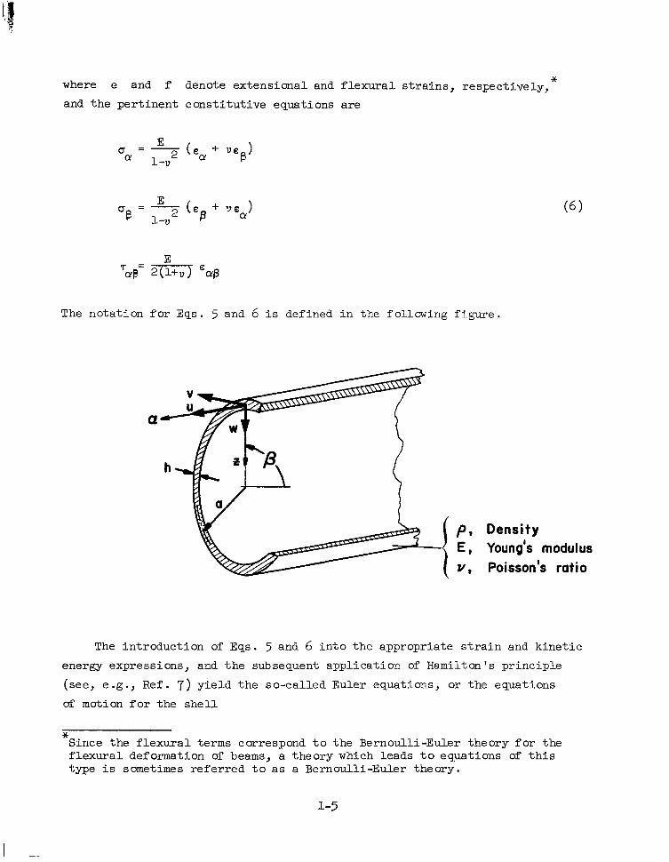
where e and f denote extensional and f l exura l s t r a ins , r e spec t ive ly ,

and the per t inent cons t i tu t ive equat ions a re

*

The no ta t ion fo r Eqs . 5 and 6 i s def ined in the f o l l a r ing f i gu re .

Density Young's modulus Poisson's ratio

The introduct ion of Eqs. 5 and 6 in to t he appropr i a t e s t r a in and k ine t i c

energy expressions, and the subsequent application of Hamilton's principle

(see, e.g., R e f . 7 ) yield the so-cal led Euler equat ions, or the equations

of motion f o r t h e s h e l l

* Since the f lexural terms correspond to t he Be rnou l l i -Eu le r t heo ry fo r t he f lexural deformation of beams, a theory which leads t o equations of t h i s type i s sometimes r e f e r r e d t o a s a Bernoulli-Euler theory.

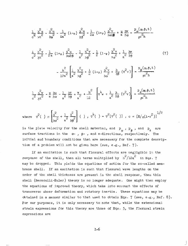
i s the p l a t e ve loc i ty fo r t he she l l ma te r i a l , and p a , Pp ? and Pz a re

su r face t r ac t ions i n t he a- , p- , and z-direct ions, respect ively. The

i n i t i a l and boundary condi t ions tha t a re necessary for the complete descr ip-

t i o n of a problem will not be given here (see, e .g., Ref. 7 ) .

I f an exc i t a t ion i s such that f l e x u r a l e f f e c t s a r e n e g l i g i b l e i n t h e

response of the she l l , then a l l t e rms mul t ip l ied by h2/12a i n Eqs. 7 may be dropped. This yields the equations of motion for the so-ca l led mem-

brane shel l . If an exc i t a t ion i s such t ha t f l exu ra l wave lengths on the

order of the she l l th ickness a re p resent in the she l l response , then th in

shel l (Bernoul l i -Euler) theory i s no longer adequate. One might then employ

the equations of improved theory, which take in to account the e f fec ts of

transverse shear deformation and r o t a t o r y i n e r t i a . These equations may be

obtained in a manner s i m i l a r t o t h a t used t o o b t a i n Eqs . 7 (see, e .g., Ref. 8) . For our purposes, it i s only necessary t o note that , whi le the extensional

s t ra in express ions for th i s theory a re those of Eqs . 5 , t h e f l e x u r a l s t r a i n

expressions are

2

1-6

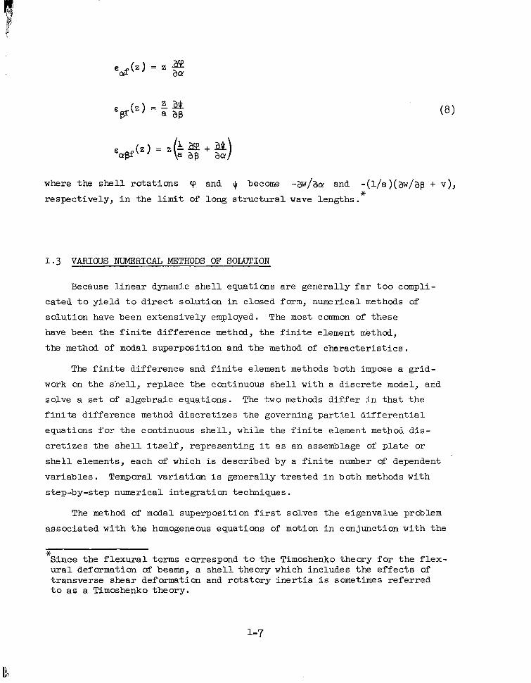
where the shell ro t a t ions cp and Jr become -aw/act and -(l/a)(aw/ag + v) ,

r e spec t ive ly , i n t he limit of long s t ruc tura l wave lengths . *

1.3 VARIOUS NUMERICAL METHODS OF SOLUTION

Because l i n e a r dynamic she l l equa t ions a r e gene ra l ly f a r t oo compli-

cated t o y i e l d t o d i r e c t s o l u t i o n i n c l o s e d form, numerical methods of

solut ion have been extensively employed. The most common of these

have been t he f i n i t e d i f f e rence method, t h e f i n i t e element method,

the method of modal superposit ion and the method of cha rac t e r i s t i c s .

The f i n i t e d i f f e r e n c e and f i n i t e element methods both impose a g r id -

work on the shel l , replace the cont inuous shel l wi th a d i s c r e t e model, and

solve a s e t of a lgebraic equat ions. The two methods d i f f e r i n t h a t t h e

f i n i t e d i f f e r e n c e method d iscre t izes the govern ing par t ia l d i f fe ren t ia l

equat ions for the cont inuous shel l , whi le the f ini te e lement method d i s -

c r e t i z e s the s h e l l i t s e l f , r e p r e s e n t i n g it as an assemblage of p l a t e or shell elements, each of which i s described by a f i n i t e nuniber @ dependent

va r i ab le s . Temporal v a r i a t i a n i s gene ra l ly t r ea t ed i n bo th methods with

step-by-step numerical integration techniques.

The method of modal superposit ion f i r s t solves the eigenvalue problem

associated with the homogeneous equations of motion in conjunct ion with the

* Since the f lexura l terms correspond t o t h e Timoshenko t h e o r y f o r t h e f l e x - ural deformation of beams, a she l l t heo ry which inc ludes the e f fec ts of transverse shear deformation and r o t a t o r y i n e r t i a i s sometimes r e fe r r ed t o a s a Timoshenko theory.

1-7

governing boundary conditions. The r e s u l t i n g s h e l l modes are then used t o construct the forced motion of the she i l by l inear superpos i t ion . The method

of charac te r i s t ics requi res hyperbol ic she l l equa t ions (Eqs . 7 a r e of the

parabol ic type with regard to f lexural motion) and therefore makes use of

improved (Timoshenko) she l l t heo ry . The she l l equa t ions a r e t hen r ecas t i n

terms of the appropr ia te charac te r i s t ics and solved numerically.

*

All of the above methods share a common f a i l i n g , namely, the use of a

f i n i t e number of response var iables to represent cont inuous funct ions. Their

success depends , therefore , upon the ra te of convergence of their numerical

so lu t ions w i th r e spec t t o f i n i t e i nc reases i n t he number of response variables

(degrees-of-freedom) and the e f f ic iency wi th which they e f fec t the necessary

computations f o r a given number of response variables. Generally speaking,

t h e f i n i t e d i f f e r e n c e and f i n i t e element methods are numerically the most

e f f i c i e n t f o r a given number of response variables; the method of modal

superposit ion i s l e s s e f f i c i en t , bu t o f t en r equ i r e s a smaller number of r e -

sponse var iab les and provides modal information that need only be generated

once for multiple response computations; the method of cha rac t e r i s t i c s i s

t h e l e a s t e f f i c i e n t method, but, because it embodies the essent ia l charac te r -

i s t i c s of wave propagation behavior, it can accu ra t e ly t r ea t sno r t wave length

response , including response discont inui t ies . Thus , a dec i s ion a s t o which

method should be used t o solve a pa r t i cu la r problem can only be based on the

nature of the problem i t s e l f . (For a comprehensive assessment of current

she l l ana lys i s capabi l i ty , see Ref . 9.)

1 . 4 THE STAR CODE: DESCRIPTION AND APPLICATION . . - " .

The STAR (Shel l Transient Asymmetric Response ) computer program can be

used f o r t h e two-dimensional, nonlinear, transient response analysis of in -

e las t ic she l l s wi th unre inforced cu touts . A detai led discussion of the code

i s given i n t h e U s e r ' s Manual f o r STAR (Ref. 10). Improvements made i n t h e

code a s pa r t of the present s tudy are descr ibed in Appendix A .

3f- For complicated geometries, the homogeneous equations of motion are usual ly so lved wi th f in i te d i f fe rence or f i n i t e element methods.

1-8

The STAR code i s based on the genera l th in she l l equa t ions of R e f . 6, which inc lude nonl inear . gemet r ic terms, and on a set of cons t i t u t ive equa-

t i o n s f o r a temperature-dependent, work-hardening material. Lines of p r in -

c ipal curvature are used for the curvi l inear coordinates (a,p) of the middle

surface of t h e s h e l l . (See Appendix A fo r no ta t ion and sign conventions. ) The basic solution procedure employed by the code i s as fol lows. The govern-

i n g p a r t i a l d i f f e r e n t i a l e q u a t i o n s of motion are reduced t o a set of time-

dependent ordinary differential equations by the application of two-dimensional

f in i te d i f fe rence approximat ions for der iva t ives w i t h r e s p e c t t o t h e s h e l l ' s

middle surface coordinates a and p . An e x p l i c i t ( c e n t r a l ) f i n i t e d i f f e r -

ence numerical integration scheme i s then employed f o r t h e s o l u t i o n of t he

ord inary d i f fe ren t ia l equa t ions .

Solutions obtained with t h e e x p l i c i t scheme are numerical ly s table if

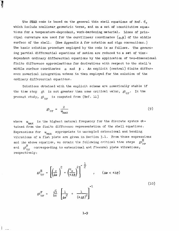
the t ime step A t i s not greater than some c r i t i c a l Value, atcr. In t he

present study i s computed from (Ref. 11) Atcr

where w i s the highest natural f requency for the discrete system ob-

ta ined from the f i n i t e d i f f e rence r ep resen ta t ion of the shel l equat ions.

Expressions for appropriate t o uncoupled extensional and bending

v ibra t ions of a f l a t p l a t e a r e given in Sec t ion 3.1. From those expressions

and the above equation, we obta in the fo l luwing c r i t i ca l t ime s teps

and Atc, corresponding t o e x t e n s i o n a l and f l exura l p l a t e v ib ra t ions ,

respec t ive ly :

max

wmax

E Atcr F

following consideration. Let h denote a c h a r a c t e r i s t i c s t r u c t u r a l wave

length appropriate to nondispersive, axisymmetric'.wave propagation i n t h e

s h e l l . Then, f o r problems with in-plane exci ta t ions, was s e l e c t e d i n

accordance with the cri terion Aa/h << 1. It was f o u n d t h a t t h i s c r i t e r i o n

cons is ten t ly gave good r e s u l t s , s o it s e r v e d a s t h e b a s i s f o r a l l problems

characterized by predominantly in-plane excitations.

For problems with transverse loadings, ~a was selected in accordance

wi th the c r i te r ion tha t Aa/h N 1 , where h i s the she l l th ickness . A

more sophis t icated method f o r choosing A~CU evolved during the course of

the present study. This method i s discussed in Chapter 3. In the so lu t ion

of asymmetric problems, the mesh a s p e c t r a t i o (Aol/aAp) was s e l e c t e d t o be

on the order of uni ty .

One of the major considerations used i n t h e s e l e c t i o n and execution of

the problems of the next chapter was that the computation time for a s ingle

problem should be less than five minutes. The following approximate ex-

pression was used t o estimate computation times on the Univac 1108 fo r bo th

axisymmetric and asymmetric response problems :

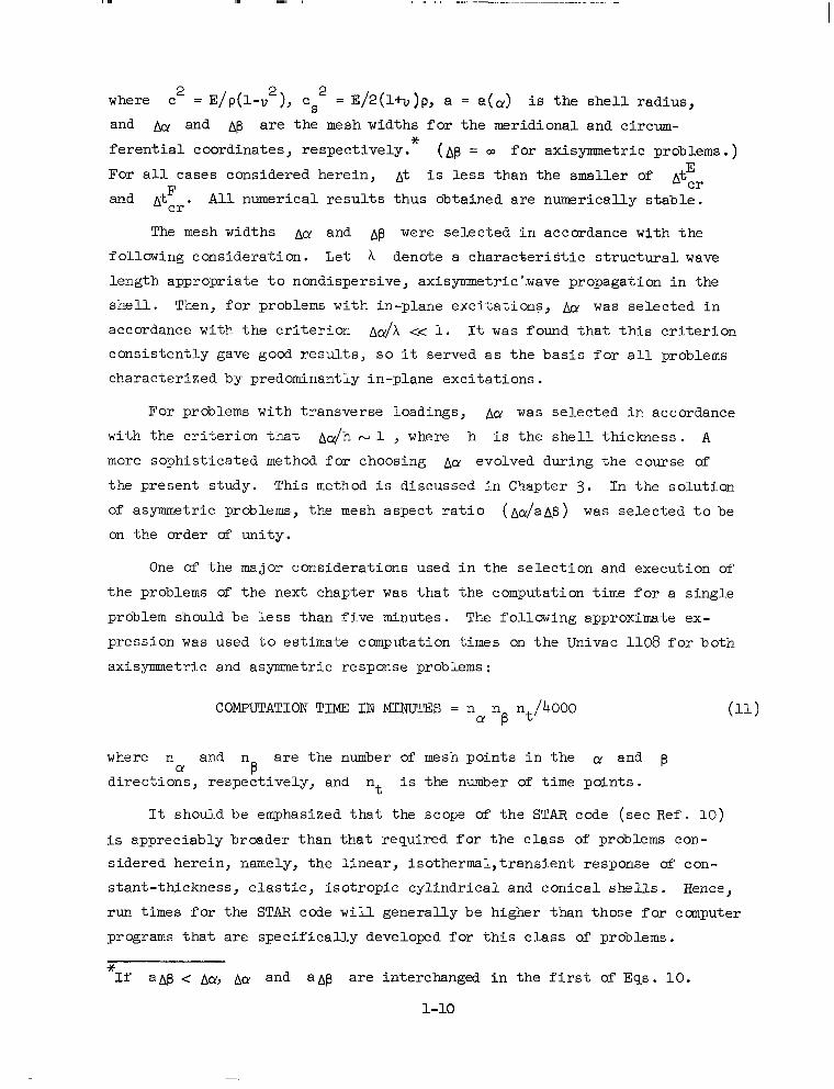
COMPUTATION TIME IN m m s = n n n /bo00 D e t

(11 1

where n and n a r e t h e number of mesh p o i n t s i n t h e and p direct ions, respect ively, and n i s the nurdber of t ime points . t

CY B

It should be emphasized that the scope of t he STAR code (see Ref. lo)

i s apprec iab ly b roader than tha t requi red for the c lass of problems con-

sidered herein, namely, the l inear, isotherma1,transient response of con-

s tan t - th ickness , e las t ic , i so t ropic cy l indr ica l and con ica l she l l s . Hence,

run t imes for the STAR code w i l l general ly be higher than those for cmputer

programs t h a t a r e s p e c i f i c a l l y developed f o r t h i s c l a s s of problems.

* If a Ap < Aa, AD and a A$ are interchanged in the f i r s t of Eqs . 10.

1-10

Chapter 2

NUMERICAL STUDY OF CONVERGENCE

I n this chapter, we investigate numerically the convergence of f i n i t e

d i f fe rence t rans ien t wave propagation computations. Because we a r e p r i -

mari ly interested in propagat ion a long the meridional coordinate , most of

the cases involve axisymmetric response, although problems with gentle

asymmetry a re a l so i nc luded .

To f a c i l i t a t e our study, l e t u s de f ine fou r exc i t a t ion c l a s s i f i ca t ions .

The f i r s t c l a s s i f i c a t i o n i s (z, r), which inc ludes exc i ta t ions tha t a re

broad in the meridional dimension a and gradual in the temporal dimension

t . The second c l a s s i f i c a t i o n i s (& r), which cons is t s of exc i ta t ions

t h a t a r e narrow i n b u t g r a d u a l i n t . The t h i r d i s (z, t), which in-

eludes exc i t a t ions t ha t a r e b road i n (Y bu t ab rup t i n t . The f i n a l c l a s s i f i c a t i o n i s (G, x), which cons is t s of exc i t a t ions t ha t a r e na r rm

i n (Y and a b r u p t i n t . All non-axisymmetric exc i ta t ions to be cons idered

are broad in the c i rcumferent ia l d imension p .

* +

I n o r d e r t o d e s c r i b e more prec ise ly these c lass i f ica t ions , w e define a

"spa t ia l ly b road ' ' exc i ta t ion as one tha t conta ins no s p a t i a l d i s c o n t i n u i t i e s

on an unbounded domain or one whose c h a r a c t e r i s t i c s p a t i a l dimension con-

s iderably exceeds the shel l th ickness; we define a "temporally gradual''

exc i t a t ion a s one that produces no temporal discontinuities in the velocity

response of t h e s h e l l or one whose characteristic temporal dimension con-

siderably exceeds the transit t ime of an extensional wave through the shel l

thickness . The terms "spatially narrow" and "temporally abrupt" are, of

course, just the opposite of the above de f in i t i ons . Because the imposit ion

of boundary conditions i s equ iva len t t o t he app l i ca t ion of l i n e l o a d s t o a

she l l , any disturbance reaching a s h e l l boundary gives rise t o an exc i t a t ion

t h a t i s s p a t i a l l y narrow i n t h e d i r e c t i o n normal t o t h e boundary. Also, spec i f i ca t ion of an i n i t i a l ve loc i ty cond i t ion cons t i t u t e s t he app l i ca t ion

of a temporal ly abrupt exci ta t ion.

The p r i n c i p a l r e s u l t s of th i s chapter a re summarized i n Table 1 on page 2-19.

* Actua l ly , exc i t a t ions i n t h i s c l a s s i f i ca t ion w i l l no t be spec i f ica l ly considered. This i s because the s tud ies per ta in ing to the o ther c lass i f ica t ions demonstrate t h a t 6, y ) - excitations present no convergence problems.

2-1

2.1 DISPLACEBENT, VELOCITY AND ACCELERATION RFSPONSE TO IN-PLAN3 EXCITATION

I n this sect ion, w e examine convergence of the kinematic quant i t ies

appropr ia te to in -p lane or, more spec i f i ca l ly , l ong i tud ina l exc i t a t ion of

c y l i n d r i c a l s h e l l s .

2 .1 .1 (a, r) - Excitat ions 4

The f i r s t example involves an (z, r) - exci ta t ion in the form of a

specified bell-shaped end-displacement whose temporal width i s approximately

e q u a l t o a/2c . Thus, as d i scussed in Appendix B, (k a ) >> 1, where k

i s the wave number c h a r a c t e r i s t i c of t he l ong i tud ina l s t r a in , and a bell-shaped

displacement wave propagates with negligible dispersion down t h e s h e l l a t t h e

p l a t e ve loc i ty c .

* 2

€ L

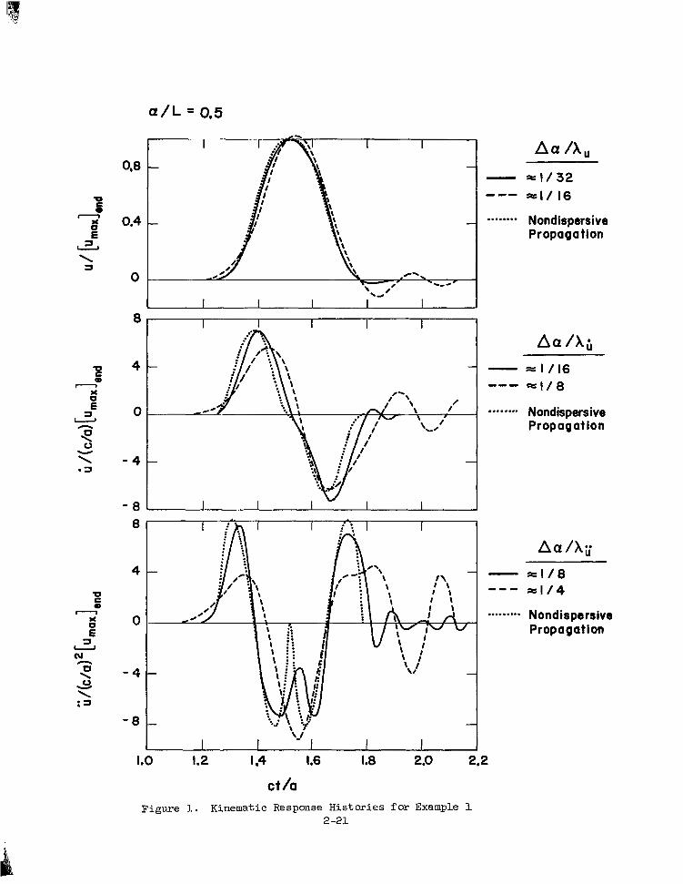
Fig . 1 shows displacement, velocity and a c c e l e r a t i o n h i s t o r i e s a t

a/L = p . We see that , because of the nature of the exc i ta t ion , t ak ing a time

derivative roughly halves the characterist ic wave length = 2rr/k. Thus,

the coarse f in i te d i f fe rence mesh i s sat isfactory for displacement computa-

t i ons bu t i s marginal for velocity computations and unsa t i s f ac to ry fo r

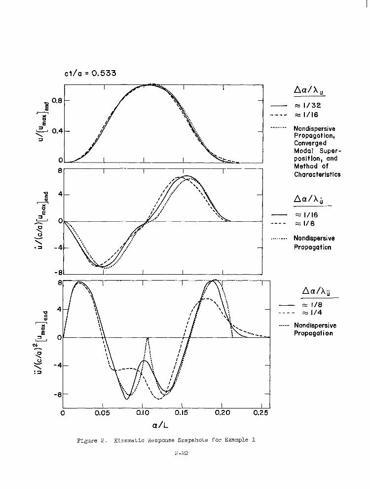
acceleration computations. Fig. 2 shows displacement, velocity and accelera-

t i on snapsho t s a t c t / a = 0.533. Because of the non-dispersive propagation,

each response snapshot i s e s s e n t i a l l y a l a t e ra l ly d i sp l aced mirror image of

t he co r re spond ing h i s to ry . Th i s desc r ip t ion ho lds a t l a t e r t imes a l so , a s

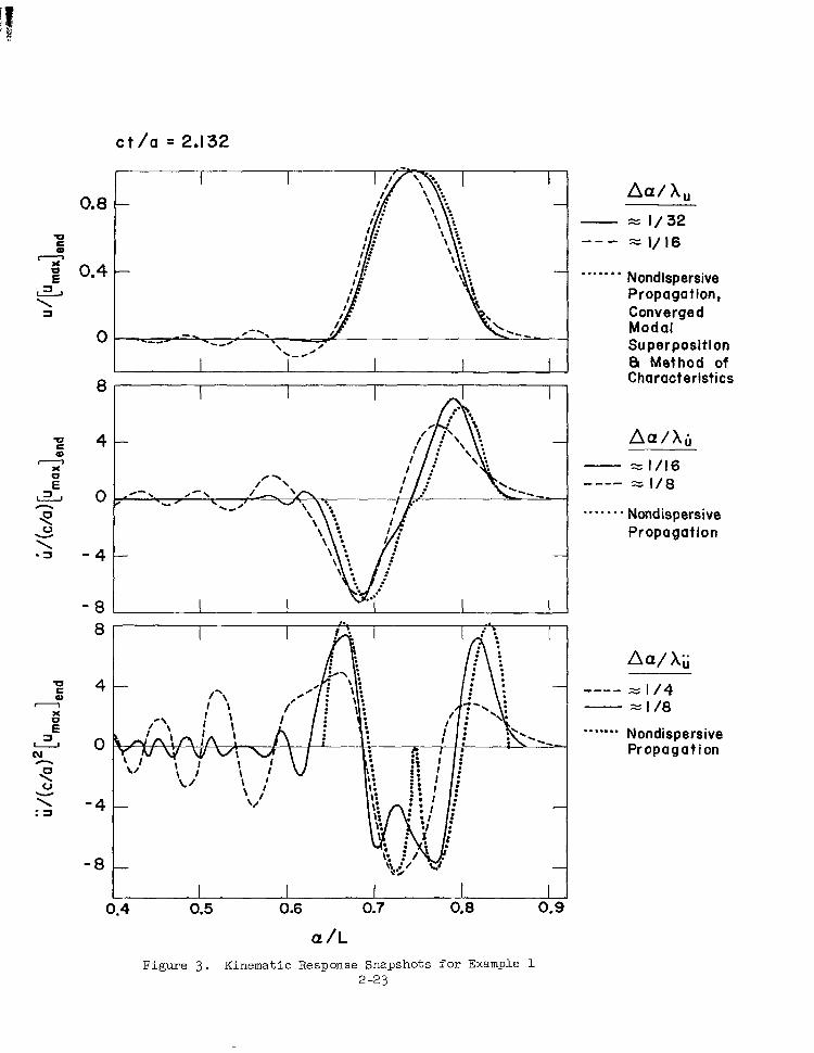
i nd ica t ed i n F ig . 3 , which shows snapshots a t c t / a = 2 . l32. Comparing

F igs . 2 and 3 , we d e t e c t , f o r a f ixed mesh width, a gradual de te r iora t ion

in accuracy as t ime increases .

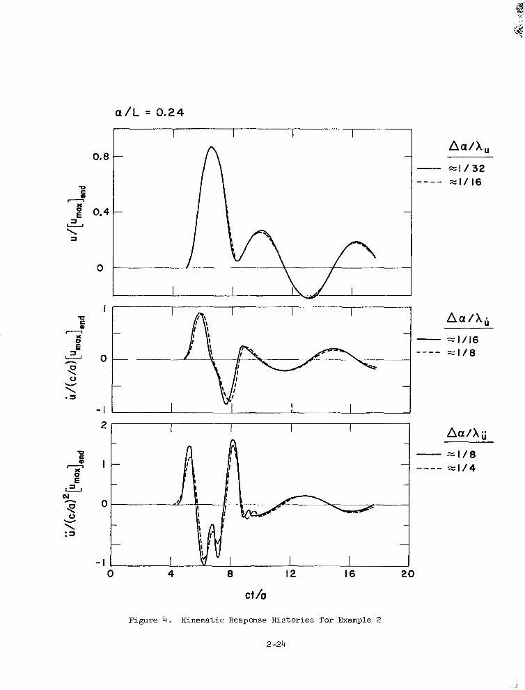
1*

The second example also involves an (& t") - exc i t a t ion i n t he form

of a specified bell-shaped end-displacement. In this case, however,

k a -1, and the wave su f fe r s s ign i f i can t d i spe r s ion a s it propagates down

the she l l ( see Appendix B ) . F ig . 4 shows displacement, velocity and €

* All the examples d i scussed i n t h i s chap te r a r e desc r ibed i n de t a i l i n Tab le 2 .

** Because, from Appendix B, 4 M - v(c/a)u, a radial response quant i ty i s smoother than the corresponding longitudinal response quantity. Furthermore, radial response i s much smaller than the corresponding longitudinal response fo r l ong i tud ina l exc i t a t ion . Thus, only longi tudinal response quant i t ies a re shown.

2-2

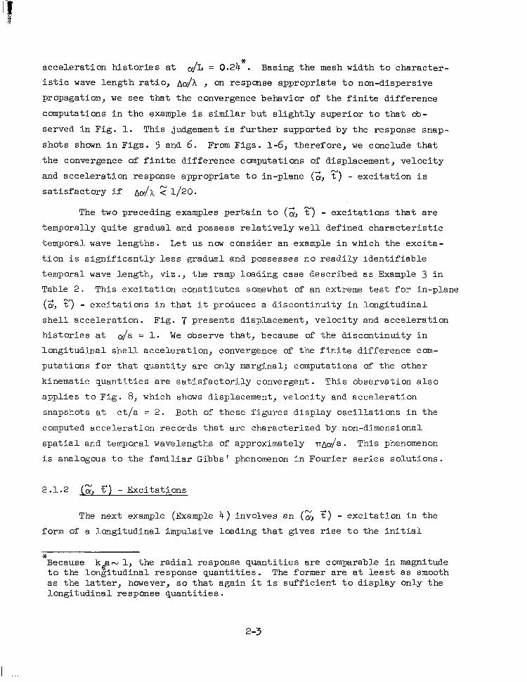
a c c e l e r a t i o n h i s t o r i e s a t dL = 0.24 . Basing the mesh width t o c h a r a c t e r -

i s t i c wave l e n g t h r a t i o , A& , on response appropriate t o non-dispersive

propagation, w e s ee t ha t t he convergence behavior of t h e f i n i t e d i f f e r e n c e

computations i n t h e example i s s imi l a r bu t s l i gh t ly supe r io r t o t ha t ob-

served i n F ig . 1. This judgement i s further supported by the response snap-

shots shown i n F i g s . 5 and 6. From Figs . 1-6, therefore , w e conclude t h a t

the convergence of f ini te difference computat ions of displacement, velocity

and acceleration response appropriate t o in-plane (& ?’) - exc i t a t ion i s

s a t i s f a c t o r y i f Aa/h 2 1/20.

*

The two preceding examples pertain t o (z, r) - exci ta t ions that a re

temporally quite gradual and possess re la t ive ly wel l def ined charac te r i s t ic

temporal wave lengths . Let us now consider an example i n which the exc i ta -

t i o n i s s i g n i f i c a n t l y l e s s g r a d u a l and possesses no readi ly ident i f iable

temporal wave length, v i z ., the ramp loading case described as Example 3 i n

Table 2 . This exci ta t ion const i tutes somewhat of an extreme t e s t fo r i n -p l ane

(z, r) - e x c i t a t i o n s i n t h a t i t produces a d i scont inui ty in longi tudina l

she l l a cce l e ra t ion . F ig . 7 presents displacement, velocity and acce lera t ion

h i s t o r i e s a t a l a = 1. We observe that, because of t he d i scon t inu i ty i n

l ong i tud ina l she l l a cce l e ra t ion , convergence of t h e f i n i t e d i f f e r e n c e com-

putations for that quantity are only marginal; computations of the other

kinematic quant i t ies are sat isfactor i ly convergent . This observat ion a lso

a p p l i e s t o F i g . 8, which shows displacement, velocity and acce lera t ion

snapshots a t c t / a = 2 . Both of t hese f i gu res d i sp l ay o sc i l l a t ions i n t he

computed acceleration records that are characterized by non-dimensional

s p a t i a l and temporal wavelengths of approximately =&a. This phenomenon

i s analogous t o t h e f a m i l i a r Gibbs phenomenon in Four i e r s e r i e s so lu t ions .

2.1.2 (a, t‘) - Exci ta t ions N

The next example (Example 4) involves an (a, 3) - exc i t a t ion i n t he N

form of a l ong i tud ina l impu l s ive l oad ing t ha t g ives r i s e t o t he i n i t i a l

* Because kea- 1, the rad ia l response quant i t ies a re comparable i n magnitude t o the longi tudina l response quant i t ies . The former are a t l e a s t a s smooth as t h e l a t t e r , however, s o tha t aga in it i s s u f f i c i e n t t o d i s p l a y o n l y t h e longi tudinal response quant i t ies .

2-3

veloc i ty d i s t r ibu t ion descr ibed in Table 2 . A s d i scussed i n Appendix B,

(k a ) >> 1 , SO t h a t t h i s example cons t i tu tes an essent ia l ly non-d ispers ive

wave propagation problem. Fig. 9 shows displacement, velocity and accelera-

t i o n h i s t o r i e s a t a dis tance a/L = 0.21 t o t h e r i g h t of the plane of loading

anti-Sp.uIIetry. We observe that , for a given Aa/), - r a t i o , convergence be-

havior i s about the same f o r this (z, 2 ) - exc i t a t ion as it i s f o r t h e (& y ) exc i t a t ion of Example 1. In o rde r t o a s su re ou r se lves t ha t s a t i s f ac to ry con-

vergence for a l l kinematic quantit ies can indeed be attained, we examine Fig.

10, which presents displacement, velocity and acce lera t ion snapshots a t

c t /a = 0.2132 and 0.8528.

2 E

The f i f t h example a l so dea l s w i th an (z, 3) - exc i t a t ion i n t he form

of a longitudinal impulsive loading which produces an i n i t i a l v e l o c i t y

condi t ion. In this case, however, k a N 1 (Appendix B ) , s o tha t t he wave

propagated a long the shel l suffers s ignif icant dispers ion. Fig. 11 pre-

sents longi tudinal d isplacement , veloci ty and a c c e l e r a t i o n h i s t o r i e s a t a

dis tance a/L = 0.12 t o t h e r i g h t of the plane of loading anti-symmetry.

The f igu re i nd ica t e s t ha t convergence i s s a t i s f a c t o r y f o r a l l q u a n t i t i e s

when Am/), << 1. This i s supported by Fig. 12, which shows displacement,

ve loc i ty and acce le ra t ion snapsho t s a t c t / a = 1.91 and 5.73. A t the

e a r l i e r t ime, dispers ion effects have not yet become s ign i f i can t , s o t h a t

the non-dispersive curves shown in the f igure cons t i tu te accura te represen-

t a t i o n s of the t rue response. This i s no longer the case, however, a t

c t /a = 5.73.

€

As Example 6, we examine an (z, 6 ) - exc i t a t ion which g i v e s r i s e t o - discont inui t ies in longi tudina l acce le ra t ion , i .e. , we consider the saw-

tooth impulse loading described in Table 2. Displacement, velocity and

a c c e l e r a t i o n h i s t o r i e s a t a l a = 2 and snapshots a t c t / a = 2 a r e shown

i n F i g s . 13 and 14, respect ively; these display the same margina l (a t bes t )

convergence in the accelerat ion computat ions that was observed i n t h e

(G, r) - exc i t a t ion example of F igs . 7 and 8.

2.1.3 (z, X) - Exci ta t ions

The seventh example deals with an (G, 3) - exci ta t ion , v iz ., a s t e p

end-veloci ty exci ta t ion. Because of t he d i scon t inu i ty i n l ong i tud ina l

shel l veloci ty , the f ini te difference computat ions for that quant i ty , as

2-4

s h a m i n F i g s . 15 and 16, are only marginally convergent. Furthermore,

because the accelerat ion can only be def ined in terms of a generalized

funct ion ( v i z . , the Di rac de l ta - func t ion) a t the wave f ron t , computations

of t ha t quan t i ty by t he f i n i t e d i f f e rence method (o r , i n f ac t , by o the r

numerical methods) are unsa t i s fac tory .

The f i n a l example of t h i s s e c t i o n (Example 8) involves a non-

axisymmetric (2, 3) - e x c i t a t i o n i n t h e form of a s tep end-veloci ty dis-

t r i bu ted as cos $ f o r - 2 5 $ 5 n/2. Figure 17 shows displacement, velocity

and accelerat ion snapshots a t c t /a = 2, $ = 0 and 90'. Comparing t h i s f i g u r e

with Fig. 15, w e observe that , for aAp/h << 1, the presence of g e n t l e a s p -

metry has no effect on general convergence behavior. The gen t l e bu t d i s t i nc t

asymmetry i s i l l u s t r a t e d i n F i g . 18, which shows kinematic response snapshots

a t c t / a = 2 and a/a = 1.

P

2.1.4 Conclusions

From Figs . 1-18, we draw the fol lowing conclusions regarding thin

s h e l l f i n i t e d i f f e r e n c e computation of she l l response to in -p lane exc i ta t ion .

F i r s t , we conclude t h a t computations of kinematic response quantit ies appro-

p r i a t e t o (& r) -, (;, t') -, and therefore (;, r) - exc i t a t ions a r e s a t i s -

fac tor i ly convergent as long as the ra t io of each spa t ia l mesh dimension t o t h e

shor tes t cor responding charac te r i s t ic spa t ia l wave length of the response i s much

less than un i ty . The value of t h e r a t i o r e q u i r e d i s determined by the length

of time f o r which solut ions are desired; the longer the t ime, the smaller

t h e r a t i o must be . Second, we conclude t h a t i f an exc i t a t ion produces a

d i scon t inu i ty i n a response quant i ty , the f ini te difference computat ion of

t ha t quan t i ty w i l l b e a t b e s t only marginally convergent due t o t h e a p p e a r -

ance of a type of Gibbs' phenomenon. Th i rd , we conclude t h a t t h e f i n i t e

d i f fe rence method cannot be used t o compute the acceleration response of

a s h e l l s u b j e c t e d t o an in-plane (z, 3) - exc i t a t ion . A s a f i n a l n o t e : It

i s f i t t i n g that fini te difference computat ions of s h e l l response appropriate

t o (2, q) - excitations possess about the same convergence behavior as those

a p p r o p r i a t e t o (z, 3 ) - excitations. Finite difference computations of an

(z, 3) - generated wave t h a t i s r e f l ec t ed from a s h e l l boundary a re t he re fo re

a s a c c u r a t e a f t e r r e f l e c t i o n a s t h e y a r e b e f o r e r e f l e c t i o n . T h i s i s because

the r e f l ec t ion of an (z, 3) - generated wave by a s h e l l boundary d i r e c t l y

2-5

corresponds to t he supe rpos i t i on of two waves: t h e (z, F) - generated

wave propagating i n t h e absence of a boundary and an (z, r) - generated

wave p r d u c e d a t t h e boundary through the enf'orcement of the boundary

condi t ion.

2.2 DISPLACEMENT, VELOCITY AND ACCELERATION RESPONSE TO TRANSVERSE EXCITATION ~ . . " . " -~ ~

The propagation of waves generated by transverse excitations i s charac-

ter ized by severe dispers ion. We are therefore denied here the simple

s p a t i a l wave length descr ipt ions embodied i n many of the preceding examples.

Thus we deal immediately with transverse excitations that introduce no

well-defined characterist ic temporal or s p a t i a l wave lengths , bu t which

are mathematically simple.

2.2.1 ( G , r) - Excitat ion

The f i r s t example of t h i s s e c t i o n , Example 9, involves the (z, c) - exc i t a t ion of a clamped-clamped cy l ind r i ca l she l l by a uniform, r a d i a l s t e p -

pressure. That this problem cons t i tu tes a simple (& r) f l e x u r a l wave

propagation problem i s shown by the following argument. Consider an in-

f i n i t e s h e l l e x c i t e d over i t s entire length by the uniform step-pressure;

i t s response i s given by w ( a , P , t ) = w ( t ) = (Poa /phc ) (1 - cos c t /a ) ,

where Po i s the magnitude of the pressure s tep. Now consider an ident ical

in f in i te she l l exc i ted ax isyrmnet r ica l ly a t a = 0 and (Y = L by the pre-

scribed radial displacements w ( 0 , p , t ) = w(L, p , t ) = - w , ( t ) . Since the

combination of these two problems yields the problem of Example 9, and

s ince the un i formly exc i ted in f in i te she l l problem embodies no f l e x u r a l

wave e f f e c t s , Example 9 does cons t i t u t e a simple (2, r) f l e x u r a l wave prop-

agation problem.

2 2 m

Fig . 19 shows displacement, velocity, and a c c e l e r a t i o n h i s t o r i e s a t

d L = - f o r Example 9. We see that , while displacement and velocity con-

vergence may be termed sa t i s f ac to ry , convergence of the acce le ra t ion com-

putat ions is , a t best , marginal . This convergence diff icul ty i s analogous

1 * 2

* Longitudinal responses computed a t o t h e r s t a t i o n s a l o n g t h e s h e l l proved t o be smaller and general ly smoother than the corresponding radial responses.

2-6

t o t h a t of the previous section, which was associated with a d i scont inui ty

a t t he ex t ens iona l wave f r o n t . A s impl ied in Sec t ion 1.3, we cannot assoc-

ia te the p ropagat ion of a wave front with the e lementary (Bernoul l i -Euler)

f lexural equat ions. To do t h i s , we employ improved (Timoshenko) theory

that in t roduces an extensional wave f r o n t t r a v e l l i n g a t v e l o c i t y

c = [E/~(l-u~]]~/~ and a shear wave f r o n t t r a v e l l i n g a t v e l o c i t y

c S = f$,/2p(l+v)]1/2, where W, i s the shear fac tor (0.8 <" W, <. 1.0) .

On this bas i s , w e see tha t the h igh- f requency osc i l la t ions i n t he Aa/h = 1

accelera t ion h i s tory of F ig . 19 appear t o beg in w i th t he a r r iva l of two

acce lera t ion d i scont inui t ies (one from each end) that travel a t c and

s imul taneous ly reach the she l l ' s mid-s ta t ion a t c t /a w 2 (see, e .g., Ref.

13). A shor t t ime la te r , the acce le ra t ion h i s tory smooths out, only t o b e

disrupted again upon the second a r r iva l a t c t /a M 6 of the acce le ra t ion

d i scon t inu i t i e s , which have been r e f l ec t ed from the ends of t h e s h e l l .

This in te rpre ta t ion i s supported by the Aa/h = 1 curves of Figs . 20 and

21, which show displacement, velocity and accelerat ion snapshots a t

c t /a = 1.2 and 4.8, respec t ive ly . The analogy between th is behavior and

t h a t of the previous subsection i s more completely established by com-

parison of F igs . 19 and 7.

S

While the Ao/h = 1 computations appear t o p r e d i c t w i t h some degree

of accuracy the a r r iva l of an acceleration discontinuity, the computations

for o ther va lues of Aa/h e i ther ignore i t s a r r i v a l or, in the case of

the Aa/h = - computations , p r e d i c t t h e a r r i v a l of a f l e x u r a l wave with

a ve loc i ty even grea te r than the d i la ta t iona l ve loc i ty . This is in cont ras t

to the case involv ing in -p lane exc i ta t ion , where changes i n the value of

Ao/h Produce no such r a d i c a l changes i n t h e computed responses (see Fig. 7). We conclude, therefore , that the less than sat isfactory convergence of the

f ini te difference accelerat ion computat ions i s due t o t h e i n a b i l i t y of

elementary bending theory t o t r e a t p r o p e r l y t h e s h o r t wave length components

contained in the accelerat ion response. The USE. of a f i n i t e d i f f e r n e e code

based on improved theory should mater ia l ly inprove this s i tuat ion, even

though the problem of dealing numerically with a response discontinuity

would s t i l l be present.

1 2

* * The modal superposit ion acceleration snapshots of F igs . 20 and 21, which a re computed f r m 180 m d a l r e s p o n s e s a p p r o p r i a t e t o improved she l l theory (Ref . 15), cannot be accurate in the vicinity of t he acce le ra t im d i scon t inu i ty e i the r ; this problem w i l l b e d i s c u s s e d i n g r e a t e r d e t a i l l a t e r .

2-7

. . . . .. . ""

2.2.2 (z, 3) - Exci ta t ion

The next example, Example 10, involves the (z, <) - exc i t a t ion of the

clamped-clamped c y l i n d r i c a l s h e l l of Example 9 by an axisymmetric, triangular

radial impulse. Fig. 22 shows displacement, velocity and acce lera t ion his-

t o r i e s a t OJL = - As i n t he p rev ious example, convergence of the d i s -

placement and velocity computations i s sa t i s f ac to ry , whereas convergence of

the acceleration computations i s , a t bes t , marg ina l . T h i s i s a l s o r e f l e c t e d

in F igs . 23 and 24, which show displacement, velocity and acceleration snap-

s h o t s a t c t / a = 1 .2 and 4.8, respec t ive ly . We observe f rom the l a t te r tha t

the lack of convergence i n the acceleration computations persists even at

r a the r l a t e t imes . The problem i s a l l ev ia t ed somewhat i f the d i scont inui ty

i n t h e s p a t i a l d e r i v a t i v e of the i n i t i a l v e l o c i t y d i s t r i b u t i o n i s reduced.

T h i s i s demonstrated i n F i g . 25, which presents displacement, velocity and

acce le ra t ion h i s to r i e s a t o/L = f o r t h e s h e l l of Example 10 excited by

an axisy-mmetric t r i a n g u l a r r a d i a l impulse whose base i s twice as wide a s

tha t appropr ia te to F ig . 22 .

1* 2 .

1

2.2.3 (G , 3) - Exci ta t ions

We now proceed t o an example (Example 11) that involves an (G, x ) - e x c i t a t i o n i n t h e form of a u n i f o r m r a d i a l impulse applied t o t h e clamped-

clamped c y l i n d r i c a l s h e l l of Example 9. It i s eas i ly seen that the d i s -

placement and velocity responses of t h i s example a r e i d e n t i c a l t o t h e

ve loc i ty and acceleration responses, respectively, of Example 9 (Figs .

19-21), Hence the discussion of the l ack of convergence in t he acce le ra -

t i o n computations of Example 9 d i rec t ly appl ies to the ve loc i ty computa t ions

of t h i s example. We show the displacement and veloci ty responses as well

as an acce le ra t ion h i s tory and two acce lera t ion snapshots for th i s example

i n F i g s . 26-28; these f igures demonstrate t ha t convergence of t h e f i n i t e

difference acceleration computations i s c l ea r ly unsa t i s f ac to ry . The i m -

proved theory modal superposi t ion computat ions are a lso suspect , in view

of t he d i scon t inu i ty i n t he she l l ' s ve loc i ty r e sponse .

* Again, longitudinal responses computed a t o t h e r s t a t i o n s a l o n g t h e she l l proved t o be smaller and generally smoother than the corresponding radial responses.

2-8

I n o r d e r t o assess t h e e f f e c t s of v a r i a t i o n s i n (2, 3) - exci ta t ions ,

w e consider as Example 12 the problem of the previous example wi th the clamped

supports changed t o f r e e s u p p o r t s . D i s p l a c e m n t , v e l o c i t y and acce lera t ion

h i s t o r i e s a t d L = 1/4 a r e shown i n F i g . 29 t o demonstrate the smoothness

of the longi tudina l responses in re la t ion to the cor responding rad ia l re -

sponses. For these 5oundary conditions, longitudinal response i s comparable

i n magnitude t o r a d i a l r e s p o n s e , a s i t u a t i o n t h a t does not occur in t he ca se

of clamped boundaries. Fig. 30 shows radial d isplacement , veloci ty and acce l -

e r a t i o n h i s t o r i e s a t a/L = 1/2; comparing these resul ts wi th those of F ig .

26, we see t ha t t he change i n boundary conditions has no e f fec t on the con-

vergence behavior of the f in i te d i f fe rence computa t ions . This i s a l s o

demonstrated i n F i g s . 31 and 32, whicn show disp lacemnt , ve loc i ty and

acce lera t ion snapshots a t c t /a = 1.2 and c t /a = 4.8, respec t ive ly .

As Example 13, we examine the non-axisymmetric response of a clamped-

clamped c y l i n d r i c a l s h e l l t o an (;, 3) - exc i t a t ion i n t he form of a longi-

tudinal ly uniform radial impulse that i s d i s t r ibu ted a s cos $ over the

region -n/2 5 $ < n/2. I n o r d e r t o e v a l u a t e b e t t e r t h e e f f e c t s of gent le

asymmetry, displacement, velocity and a c c e l e r a t i o n h i s t o r i e s a t a/L = 0.50

a re shown i n F i g . 33 for the associated axisymmetric problem involving a

uniform radial impulse. The l e s s t h a n s a t i s f a c t o r y convergence of the ve-

l o c i t y and acceleration computations i s again apparent. Fig. 34 shows d i s -

placement, velocity and acceleration histories for the cosine radial impulse

problem a t a/L = 0.50 and $ = 0. The differences between these r e su l t s

and those of Fig . 33 a re minor. F ig . 35, which shows corresponding histories

a t a/L = 0.50 and $ = 909 demonstrates t h a t t h e convergence behavior of

the axisymmetric and $ = 0 r e s u l t s a l s o c h a r a c t e r i z e s t h e r e s u l t s a t p o i n t s

on t h e s h e l l that a re no t d i r ec t ly exc i t ed . The gen t l e bu t d i s t i nc t asym-

metry of the cosine impulse problem i s i l l u s t r a t e d i n F i g . 36, which shows

displacement, velocity and acceleration snapshots a t c t / a = 0.78 and

a/L = 0.50. The A0(lh = 0.92 and 1.73 r e s u l t s a g r e e w e l l a t t h i s e a r l y

time; from Figs . 34 and 35, however, we s e e t h a t t h e s e r e s u l t s b e g i n t o

diverge a shor t t ime la te r . F ina l ly , F igs . 37 and 38 show displacement,

ve loc i ty and acce lera t ion snapshots a t c t /a = 0.78 f o r t h e uniform impulse

problem and a t c t / a = 0.78, $ = 0 for the cosine impulse problem,

respec t ive ly . As with Figs . 33 and 34, these computat ions display vir tual ly

2-9

ident ica l behavior . We conclude from Figs. 33-38, t h e r e f o r e , t h a t f i n i t e

difference response computations for gently non-axisymnetric excitations

d isp lay the same convergence behavior as those for corresponding axisymmetric

exc i t a t ions .


The three preceding examples have demonstrated that, because of the

l imi t a t ions of the elementary bending theory on which they are based and

because of t h e i r i n a b i l i t y t o t r e a t p r o p e r l y r e s p o n s e d i s c o n t i n u i t i e s ,

convergence of the f ini te difference computat ions of ve loc i ty and accelera-

t ion responses t o (2, 3) - exc i t a t ions a r e l e s s t han s a t i s f ac to ry . It i s

of i n t e r e s t , t h e n , t o examine two methods f o r modifying the excitation s o

as t o a m e l i o r a t e t h i s s i t u a t i o n .

The f i r s t method cons is t s of smoothing the exci ta t ion temporal ly ,

e .g . , converting the impulsive loading of Example 12 i n t o a pressure load-

ing of small, bu t f i n i t e , du ra t ion . Such a conversion i s shown as Example 1 4 i n Table 2. Displacement, velocity and acce lera t ion h i s tor ies appropr ia te

t o t h e l o a d d u r a t i o n c t /a = 0.82 a r e shown i n F i g . 39. This duration i s

much less than the per iod @/a = 277 of the s inusoidal response appropriate

t o t h e a s s o c i a t e d problem of an impuls ive ly exc i ted in f in i te she l l . Hence

the displacement response of F ig . 39 agrees qu i te wel l wi th tha t of F ig . 30, once the former i s moved t o t h e l e f t a d i s t a n c e c t /a = 0.41 t o a l low for

tk f i n i t e d u r a t i o n of the t r iangular pressure loading. Convergence of the

ve loc i ty and acceleration computations of F ig . 39 i s much b e t t e r t h a n t h a t

of Fig. 30, however; we observe that smoothing even allows us t o use the

ve ry f i ne mesh Aa/h = without introducing the high-frequency oscil lations

encountered i n Aa/h = 1 acceleration computation of Fig. 30 . S t i l l f u r t h e r

improvement i n convergence behavior i s achieved i f the width of t he t r i angu la r

pressure loading i s i n c r e a s e d t o c t /a = 1.64, a s shown i n F i g . 40. If the

time s h i f t c t /a = 0.82 i s in t roduced in to these resu l t s , even th i s tempor-

a l ly r a the r b road exc i t a t ion cons t i t u t e s a reasonable approximation t o t h e

impulsive exci ta t ion of Example 12.

W

S

1

W

S

The e f f e c t s of temporal smoothing are even more clearly demonstrated

i n F i g . 41, which shows ve loc i ty and acce le ra t ion snapsho t s a t c t / a = 1.2

f o r t h e s h e l l of Example 12. Shown a re 1) response snapshots for a uniform

2-10

impulse loading as computed with the modal superposit ion method based on

improved theory, and 2 ) response snapshots for a s p a t i a l l y uniform triangular pressure loading of width c t /a = 0.40 a s computed w i t h t h e f i n i t e

difference method based on elementary theory. From t h i s f i g u r e and Fig . 31, we see t h a t t h e r e i s much b e t t e r agreement between t h e f i n i t e d i f f e r e n c e

responses appropriate t o t he t r i angu la r p re s su re l oad ing and the modal super-

posi t ion solut ions than between the la t ter and the f i n i t e d i f f e rence so lu -

t i o n s a p p r o p r i a t e t o t h e impulse loading.

W *

The second method f o r improving the convergence of f in i t e d i f f e rence

computations of ve loc i ty and acce lera t ion responses to (2, t") - exc i t a t ions

cons is t s of smoothing the exc i t a t ions spa t i a l ly . For example, we might con-

vert the uniform impulsive loading of Example 12 i n t o an axisymmetric impul-

sive loading which cons t i tu tes a t runcated Fourier ser ies expansion (s in mna/L)

of the longitudinally uniform loading, as shown a s Example 15 in F ig . 42 .

Displacement , veloci ty , and accelerat ion his tor ies a t a/L = - f o r m = 5 1 2 max

are shown i n F i g . 43; we observe that convergence i s s a t i s f a c t o r y f o r a l l

th ree responses . S imi la r h i s tor ies for mmax = 11 are shown i n F i g . 44; here we must make ve loc i ty and acceleration computations with Aa/h = 1/2

t o demonstrate satisfactory convergence. Fig. 45 shows comparable h i s t o r i e s

f o r m = 23; a t t h i s p o i n t we f i n d t h a t t h e convergence of the d i sp lace-

ment, ve loc i ty and acceleration computations i s sat isfactory, marginal and

unsat isfactory, respect ively. Thus, f o r m = 23 , we have e s s e n t i a l l y

the same convergence s i t u a t i o n a s t h a t shown in Fig. 30 for the uniform

impulsive loading.

max

max

2.2.5 Conclusions

From Figs . 19-45, we draw the fol lowing conclusions regarding thin

she l l f in i te d i f fe rence computa t ion of she l l response to t ransverse ex-

c i t a t i o n . F i r s t , we conclude that computations of displacement and ve loc i ty

response appropr ia te to ( z , r) -, (z, 3) -, and therefore (z, r) - exc i t a t ions

a re sa t i s fac tor i ly convergent a s l ong a s t he r a t io of each spa t ia l mesh

* A time s h i f t of c t /a = 0.20 has been introduced into the f ini te difference r e s u l t s t o p o s i t i o n s t h e peak of t he t r i angu la r p re s su re l oad ing a t t = 0.

2 - l l

dimension to t he sho r t e s t co r re spond ing cha rac t e r i s t i c spa t i a l wave length of

the response i s appreciably less than uni ty . The convergence of t ransverse

acceleration computations, however, i s only marginal f o r (G, r) - and

(z, 2) - exci ta t ions , espec ia l ly when discont inui t ies are involved. Second

w e concluae that t h e convergence of f i n i t e d i f f e r e n c e c m p u t a t i o n s of

transverse displacement, velocity, and acce lera t ion response to (2, 3) - exci ta t ions i s satisfactory, marginal, and unsa t i s fac tory , respec t ive ly .

T h i s d i f f i c u l t y may be subs t an t i a l ly overcome, however, by e i ther temporal

or s p a t i a l smoothing of the exci ta t ion. Third, we conclude that the con-

vergence d i f f i c u l t i e s observed derive from two sources: the presence of

d i scon t inu i t i e s i n ce r t a in r e sponses , and t h e f a i l u r e of th in (Bernoul l i -

Euler ) she l l theory to account p roper ly for shor t s t ruc tura l wave length

response components t ha t con t r ibu te s ign i f i can t ly t o t he t o t a l r e sponse .

*

2.3 STRESS/STRAIN RESPONSE TO IN-PLANE EXCITATION

We examine here the convergence of f ini te difference computat ions of

s t ress /s t ra in response to predominant ly in-plane exci ta t ion of cy l ind r i ca l

and con ica l she l l s .

2 .3 .1 (2, r) -, (z, 3) -, and (G, 3) - Excitat ions

We f i r s t consider the (& r) - exc i t a t ion problem of Example 2,whose

kinematic shell responses were s tud ied in Sec t ion 2 .l. We sk ip Example 1

of that sect ion because, for the vir tual ly non-dispers ive propagat ion that

it d isp lays , the essent ia l ly membrane stress and strain responses are almost

d i rec t ly p ropor t iona l to the longi tudina l ve loc i ty response of t h e shell,

which has already been studied. Since Example 2 involves dispersive prupa-

gation, however, it i s of i n t e r e s t t o examine longi tudina l membrane stress

response for t h i s ca se . F ig . 46 shows membrane s t r e s s r e sponses a t a/L = 0.24, c t /a = 5.73 and c t /a = 17.2 , respectively; convergence i s seen t o b e s a t i s -

f ac to ry fo r &Ao << 1 , where i s t h e s t r e s s c h a r a c t e r i s t i c wave length

for dispers ion-free propagat ion. ho

* Although we have not observed in th i s Sec t ion any gradual de te r iora t ion in accuracy with increasing t ime, the emergence of t h i s problem i n c e r t a i n computat ions of the previous Sect ion suggest that it may occur i n computations fo r t r ansve r se exc i t a t ions also. Fortunately, the problem i s readi ly de tec ted by means of multiple computations with vari.ous mesh dimensions.

2-12

The next example i s t h e (z, r) - exc i t a t ion problem of Example 3. Membrane stress responses a t cr/a = 1 and c t /a = 2 for t h i s example

a r e shown i n F i g . 47. Because of the absence of discontinuities, conver-

gence of t h e f i n i t e d i f f e r e n c e c m p u t a t i o n s i s e n t i r e l y s a t i s f a c t o r y .

For the reason given above i n connection with Example 1, w e sk ip

Example 4 and proceed t o t h e (z, 3) - exc i t a t ion problem of Example 5. I n F i g . 48, which shows longi tudina l s t ra in responses a t a/L = 0.62,

c t /a = 1.91, and c t /a = 5.73, w e f i nd aga in t ha t convergence of t h e f i n i t e

difference computations i s s a t i s f a c t o r y f o r A ~ / A ~ < . 1.

Since the (z, 3) - exc i t a t ion of Example 6 ( the saw tooth impulse ) produces no discoutinuities in stress/strain response, convergence of the

corresponding f inite difference computations i s sa t i s f ac to ry , a s it was

f o r t h e (G? r) - exc i t a t ion of Example 3 (see Fig. 47). Thus, we omit

detailed examination of the s t ress / s t ra in responses for t h i s loading and

proceed t o t h e (2, 3) - exc i t a t ion of Example 7. Because t h i s e x c i t a t i o n

does produce d i scon t inu i t i e s i n l ong i tud ina l menibrane s t r e s s / s t r a i n r e -

sponse, convergence of the f ini te difference computat ions of such response

is , a s i n d i c a t e d i n F i g . 49, only marginal. The same i s t r u e f o r t h e

corresponding non-axisymmetric case of Example 8, a s i nd ica t ed i n F ig . 50.

2.3.2 Conclusions

From Figs . 46-50, we draw two conclusions. Firs t , w e conclude t h a t

f ini te difference computat ions of s t ress /s t ra in response to predominant ly

in-plane exci ta t ion converge sat isfactor i ly for cases involving (G, F) -, (z, 3) -, and therefore (z- r) - exc i t a t ions , a s l ong a s t he r a t io a t each

s p a t i a l mesh dimension to the shor tes t cor responding charac te r i s t ic spa t ia l

wave length uf the response i s much l e s s t han un i ty . Second, we conclude

that the convergence of these same cmputat ions appropriate to in-plane

(z? t)- exc i t a t ions i s only marginal as a r e s u l t of t he d i scon t inu i t i e s

present .

+

2.3.3 Comparison with Experimental Data

We now d i r e c t our a t t e n t i o n t o t h e comparison of f i n i t e d i f f e r e n c e

computations of s t ra in response with corresponding experimental data. The

2-13

f i r s t set of data, which derive from the exc i t a t ion of very loxg cyl indrical

s h e l l s a t one end by the imposi t ion of axisymmetric, 20 psec long, box-

shaped longi tudina l ve loc i t ies , i s described as Example 16 i n Table 2 .

S t r a i n h i s t o r i e s f o r Specimen T-1 a r e shown i n F i g . 5 1 a t = 3 inches

and 7.5 inches. We observe that, while the computations of peak s t ra in

and wave ar r iva l t ime a re accura te , the l a te t ime behavior of the experi-

mentally measured long i tud ina l s t r a in h i s to r i e s i s not accurately predicted

by the computed h i s to r i e s . S imi l a r h i s to r i e s fo r Specimens T-13 and T-14

a r e shown i n F i g s . 52 and 53; we observe that the computations of peak

s t r a in a r e a l so accu ra t e for t h e s e s h e l l s , b u t t h a t computed a r r iva l t imes

and pulse shapes are not completely satisfactory. Disagreemnt between

computed and measured pulse shapes should not be given t o o much weight,

however, because the veloci ty exci ta t ions a t the ends of t h e s h e l l s were

never actually measured; the box-veloci ty exci ta t ion i s only an assume?

input based on l e s s r e f ined measurements.

Experiments i n which the exc i ta t ions were qu i t e ca re fu l ly measured

a re repor ted in Ref . 17. These experiments, which are described a s Example 17 i n Table 2, involve the axisymmetric longitudinal excitation of a hollow cone

t h a t i s s t ruck a t t he c losed end by s t e e l b a l l s of various diameters. The

exc i ta t ions a re g iven as longi tudina l s t ra in h i s tor ies measured by a quartz

c rys t a l l oca t ed a t t he impacted end of the cone. These inputs can be ac-

curately descr ibed as

rwise , othei

S i n c e t h i s i s hardly a complete spec i f ica t ion of boundary conditions a t

the impacted end of the cone, some ana lys is i s necessary.

The mer id iona l s t ress resu l tan t for an axisymmetrically excited

con ica l she l l can be written i n t h e form

2-14

A t the impacted end of the "she l l " of Fig. 54, it seems reasonable t o t a k e

aw/& = 0 , so t h a t , a t t h a t p o i n t , - a = au/aa + t an cp aw/aa = au/aa. It a l s o seems reasonable t o t a k e u

'I - (Ulongi tudinal ) r a d i a l

= -u s i n Cp + w cos C+Y equal t o z e r o a t t h e impacted end, which makes the

term containing Poisson 's ra t io vanish. Unfortunately, the STAR code cannot

handle mixed end condi t ions l ike u s i n cp - w cos 'p = 0, s o t h a t we n m i n -

troduce an approximation. Since, for this "shell", cp = 0.175 = << n/2 , we write from Eq . 2

which i s the equivalent cyl indrical shel l aproximation. To make the

Poisson ' s ra t io t e rm vanish , then , we take w = 0 . O u r boundary con-

d i t i o n s a t t h e impacted end of the hollow cone are therefore taken as

Figure 54 shows STAR code computations of meridional membrane s t r a i n

responses along with the experimental results. The very sa t i s fac tory per -

formance of the th in she l l equa t ions used i n t h e STAR code i s su rp r i s ing

u n t i l we note that , except for the exc i ta t ion of F ig . 54d, t he s t ruc tu ra l

wave lengths character iz ing the pr imari ly longi tudinal shel l response

considerably exceed the 1/4 inch "shel l" thickness . However, even i n t h e

case of F ig . 54d, f o r which the spat ia l width of the pulse i s only about

four t imes the mesh spacing, agreement between the computed and experimental

r e s u l t s i s sa t i s fac tory . F lgure 54e shows extended results which include

bending e f f e c t s a s w e l l a s wave r e f l e c t i o n e f f e c t s from the other end of

the hollow cone. From t h i s f i g u r e , we conclude f i r s t (Gage 2 r e s u l t s ) t h a t t h e STAR code accura te ly accounts for bending e f fec ts in the hollow

cone, and second (Gage 3 r e s u l t s ) t h a t t h e f r e e edge boundary condition

2-15

assurned a t t he f a r end of t he cone i s not a very successful s imulat ion of the experimental boundary conditions, which were "not de f in i t i ve ly e s t ab l i shed"

by the experimental is ts .

2.4 STRESS/STRAIN RESPONSE TO TRANSVERSE EXCITATION

We now investigate the convergence of f ini te difference computat ions

of s t r e s s l s t r a in r e sponse i n cy l ind r i ca l she l l s t o p redominan t ly t r ansve r se

exc i t a t ions .

2.4.1 (%, r] -, (z, 3) -, and (G, 3) - Exci ta t ions

O u r f i r s t example i s Example 9, whose kinematic responses t o a t ransverse

(z, r) - exc i t a t ion were the f i r s t s tudied in Sect ion 2 .2 . Figure 55 shows

l o n g i t u d i n a l s t r a i n h i s t o r i e s a t a/L = 0 and F . We f i n d t h a t convergence

of the membrane s t r a i n computations i s uniformly satisfactory. Although we

must use the ra ther f ine mesh Aa/h = p t o ob ta in gene ra l ly accep tab le con- 1

vergence of the flexural strain computations, and although the computations

appropriate t o t h i s mesh p r e d i c t t h e a r r i v a l of a d i s turbance tha t t rave ls

f a s t e r t h a n even the dilatational velocity, convergence of t h e f i n i t e d i f -

ference canputations of f l e x u r a l s t r a i n may s t i l l be termed sa t i s f ac to ry .

This judgement i s supported by Fig. 56, which shms long i tud ina l s t r a in

snapshots a t c t / a = 1.2 and 4.8.

1*

The next example i s t h e (G, 3 ) - exc i t a t ion problem of Example 10. 1 2 ' Longi tudinal s t ra in responses a t a/L = - c t /a = 1 .2 and ct /a = 4.8 a re

shown i n F i g . 57. We conclude, on the same bas i s a s t ha t u sed i n con-

nection w i t h Figs . 55 and 56, t h a t convergence of the f i n i t e d i f f e r e n c e

membrane and f lexural s t ra in computat ions i s sa t i s f ac to ry .

We now proceed t o t h e ( G , T') - exc i t a t ion problem of Example 11.

Longitudinal strain responses of t h e s h e l l t o t h i s uniform impulse loading

a re shown i n F i g . 58. Convergence of t h e f i n i t e d i f f e r e n c e Computations f o r

* I n t h i s and subsequent examples, circumferential strain response i s s o smooth that convergence of the f ini te difference computat ions of this quant i ty i s uniformly satisfactory.

2-16

f l exura l s t r a in r e sponse i s seen t o be uniformly unsatisfactory. The m e

of Adh - r a t i o s smaller than un i ty o f fe rs no so lu t im; the resu l t ing re-

sponse computations are even more wi ld ly o sc i l l a to ry and p red ic t t he exist-

ence of disturbances which propagate a t velocit ies exceeding even the dila-

ta t iona l ve loc i ty . S ince impr wed theory predicts the propagat ion of no

d i scon t inu i t i e s i n l ong i tud ina l s t r a in r e sponse fo r ( z , 5 ) - exci ta t ions ,

t h i s convergence problem can only be associated with the short wave length

l imi t a t ions of elementary bending theory.

It i s i n t e r e s t i n g t o n o t e i n F i g . 58 t ha t ( e spec ia l ly t he results

f o r c t / a = 1 .2 ) t he t h in she l l f i n i t e d i f f e rence computa t ions seem reason-

ably accurate in regions well behind the shear wave f ront ( see the d i scuss ion

of Example 9 in Sect ion 2 .2) . This i s i n agreement with the results of other

invest igators (see, e .g., R e f . 18). A s we would expect from Section 2.2,

the convergence behavior of the f ini te difference computat ions i s unchanged

by a var ia t ion of boundary conditions. For example, changing the clamped

boundary conditions of Example 11 t o f r e e s u p p o r t boundary conditions

(Example 1 2 ) produces no improvement in t he unsa t i s f ac to ry convergence of

the f in i te d i f fe rence f lexura l s t ra in computa t ions .

We conclude t h i s subsection with a brief examination of nonaxisym-

met r ic longi tudina l s t ra in response appropr ia te to the ( z , 6) - exc i t a t ion

problem of Example 13. F ig . 59 shows l o n g i t u d i n a l s t r a i n h i s t o r i e s a t

e/L = 0.50 for the associated axisymmetric problem appropriate t o a uniform

impulse and for the cosine impulse problem a t p = 0 and p = 90". We ob-

serve the unsatisfactory convergence of the f lexural s t ra in computat ions

in a l l c a ses , no t ing e spec ia l ly t he d rama t i ca l ly p rema tu re a r r iva l of a

computed f l e x u r a l wave for Adh = 0.60. Thus, we aga in f ind that f i n i t e

difference response computations for gently non-axisymnetric problems

display the same convergence behavior a s t h a t a p p r o p r i a t e t o t h e c o r r e s -

ponding axisymmetric problems.


I n view of the unsatisfactory convergence behavior just observed,

l e t us now apply the temporal and spat ia l exci ta t ion smoothing tecMiques

discussed previously in Sect ion 2 .2 . We f i r s t cons ide r t he ca se of

2-17

Example 14, i . e . , t he app l i ca t ion of a uniform tr iangular pressure pulse.

L o n g i t u d i n a l s t r a i n h i s t o r i e s f o r a l m d d u r a t i o n c t / a = 0.82 and longi-

t ud ina l s t r a in snapsho t s fo r a l m d d u r a t i o n of c t /a = 0.40, along with

corresponding results f o r t h e impulse loading, are shown i n F i g . 6 0 . We

see that convergence of the f ini te difference computat ions i s subs t an t i a l ly

achieved for the ct/a = 0.82 tr iangular pressure loading, and that the

c t /a = 0.40 f i n i t e d i f f e r e n c e cornputations l i e c l o s e r t h a n t h o s e f o r t h e

impulse loading t c t h e impulse loading response computed wi th improved s h e l l

theory. Similar improvement i n convergence i s e f f ec t ed w i th spa t i a l smooth-

ing, as shown i n F i g . 61. T h i s f igure, which pertains t o truncated longi-

tudinal Fourier ser ies expansions of a uniform impulsive loading (Example l 5 ) , shows l o n g i t u d i n a l s t r a i n h i s t o r i e s a t a/L = F . We see t ha t convergence

i s s a t i s f a c t o r y f o r m = 5 and 11, but i s only marginal for m

1

max = 23.

m8X

2.4.3 Conclusions

From Figs . 55-61, we draw the fol lowing conclusions regarding f ini te

difference computation of s t r e s s / s t r a in r e sponse t o t r ansve r se exc i t a t ion .

F i r s t , we conclude t h a t computations appropriate t o (z, r) -, (z, 2 ) -, and 'therefore (z, r) - exci ta t ions are sat isfactor i ly convergent providing

that t h e r a t i o of each spa t i a l mesh dimension to the shor tes t cor responding

c h a r a c t e r i s t i c s p a t i a l wave length of the response i s appreciably less than

uni ty . Second, we conclude the computations appropriate t o (& 2 ) - exc i t a -

t ions a re unsa t i s fac tory , a d i f f i c u l t y which may b e p a r t i a l l y overcome,

however, by e i ther temporal or s p a t i a l smoothing of the exc i ta t ion . Thi rd ,

we conclude tha t the unsa t i s fac tory convergence encountered i s caused by

t h e f a i l u r e of t h i n s h e l l t h e o r y t o account p roper ly for shor t s t ruc tura l

wave length response components that c o n t r i b u t e s i g n i f i c a n t l y t o t o t a l r e s p o n s e .

The conclusions of Subsections 2.1.4, 2.2.5, 2.3.2 and 2.4.3 are sum-

marized and generalized i n Table 1. It i s important t o r ecogn ize t ha t t h i s

t ab l e does not indicate a t what mesh dimensions convergence w i l l be achieved,

but indicates only the convergence behavior t o be expected as the mesh d i -

mensions are reduced.

2-18

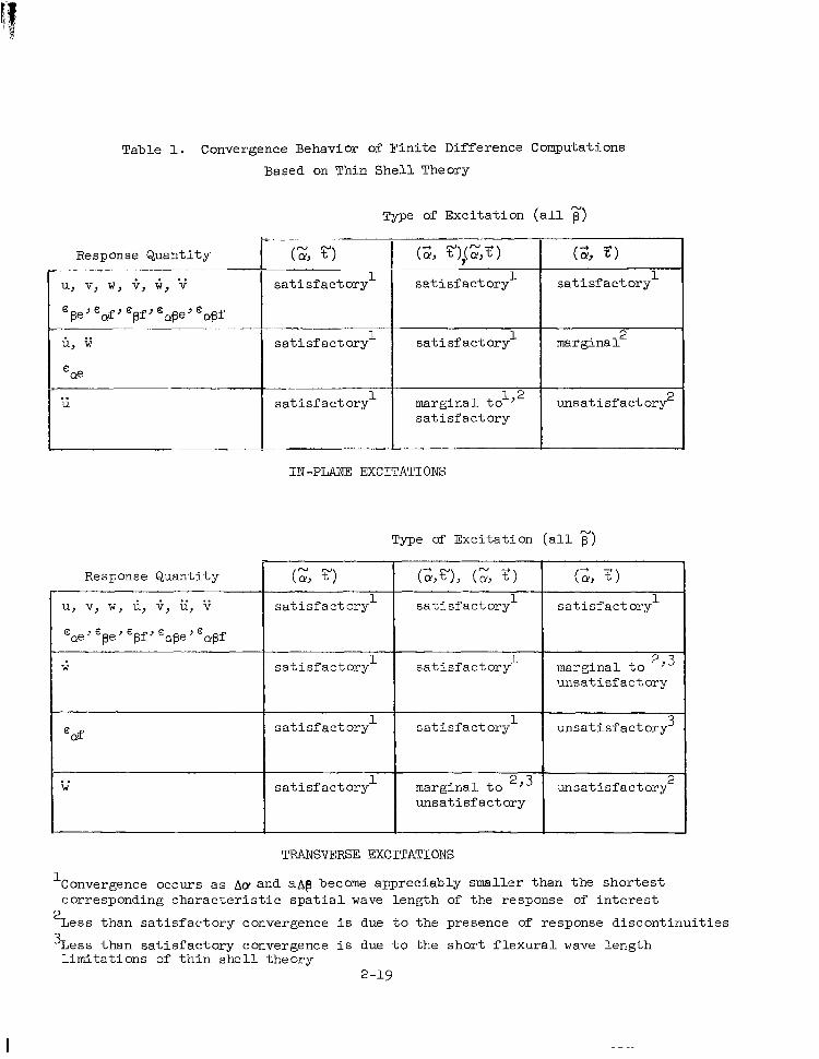
Table 1. Convergence Behavior of Finite Difference Computations Based on Thin Shel l Theory

Type of Exci ta t ion (a l l F) Response Quantity

i". - ~ "

il, w

'Qe ..

" .~

I "

(z, r) ( G J '),(;J') (;> '1 1 ~~

sat isfactory sat isfactory sat isfactory

"" "

sat isfactory marginal sat isfactory 2

I

sat isfactory unsatisfactory marginal t o 'J* 2

sat isfactory

IN-PLANE EXCITATIONS

Type of Exci ta t ion (a l l r ) Response Quantity

w

.. W

~

sat isfactory sat isfactory ~-

1

sat isfactory sat isfactory 1

sat isfactory sat isfactory 1

sat isfactory marginal to 2 ~ 3 unsatisfactory

TRANSVERSE EXCITATIONS

G, 3) sat isfactory 1

marginal t o ''3 unsatisfactory

unsatisfactory 3

unsatisfactory 2

I Convergence occws as Aa and aAfi become appreciably smaller than the shortest corresponding characteristic spatial wave length of the response of in te res t

'Less than satisfactory convergence i s due to t he presence of response discontinuities 3Less than satisfactory convergence i s due to the shor t f lexura l wave length l imitations of thin shel l theory

2-19

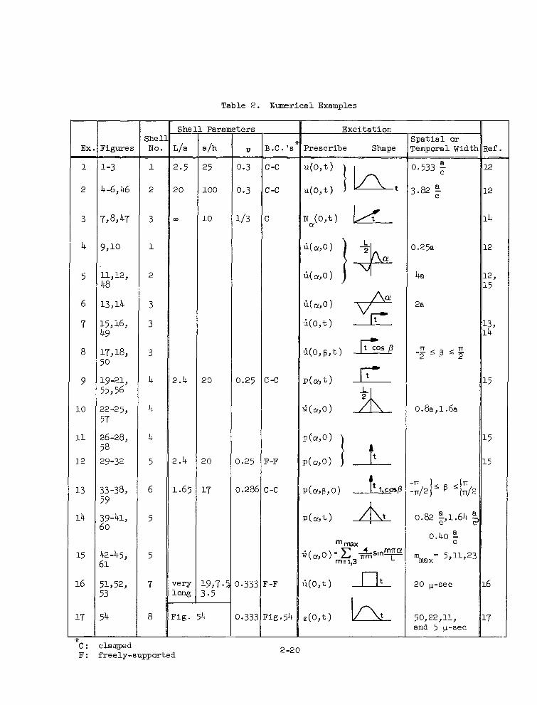
Table 2 . Numerical Examples -

Ex

1 -

2

3

4

5

6

7

8

9

10

11

12

13

14

15

16

17

Figures

1-3

4-6,46

11,12, 48

15~16, 49

1 ~ 1 8 , 50

19-21, 55,56

22-25, 57

26-28, 58 29-32

33-38, 59

39-41, 60

42-45, 51

51J52> 53

54

She 1 No.

1 - -

2

3

1

2

3

3

3

4

4

4

5

6

5

5

7

8

F: freely-supported

She

L/a - - 3.5

30

13

2.4

? .4

L .65

rery Long

vig. 54

ters

V - 0.3

0.3

1/3

0.25

3.25

0.2%

3.333

3.333

3.C. 'S

; -C

; -C

:-c

? -F

; -C

I -F

' ig .54

2-20

Exc i t a t ion

Prescribe Shape S p a t i a l o r Temporal Widtl:

0.25a

4a

2a

- - sp $ 2 rl 2

TI

o.8a,l .&

0.82 :,1.64 5 C

0.40

m = 5,11,23 max

20 p-sec

8

4

0

- 4

- 8 8

4

0

- 4

- 8

Aa /X,

- *I132 "- = I / 16

........ Nondispersive Propagatlon

........ Nondispersive Propagation

Aa /X;.

1.0 1.2 I .4 I .6 1.8 2.0 2.2

ct /a Figure 1. Kinematic Response Histor ies f o r Example 1

2 -21

- 2 1 / 8 "- X I / ~

......... Nondispersive Propagation

c? /a = 0.533

c t / a = 2.132

0.8

0.4

0

8

4

0

- 4

- 8 8

4

0

-4

-8

0.4 0.5 0.6 0.7 0,8 (

a /L Figure 3. Kinematic Response Snapshots f o r Example 1

2-23

A a / X, - 1/32 "- == 1/16

....... Nondispersive Propagation, Converged Modal Superposition S Method of Characteristics

A a / x ; - == 1/16 "" - 1/8

....... Nondispersive Propagation

Act/ x;; "" =: l / 4

= I /€I

Nondispersive Propagation

- .......

a / L = 0.24

r 0.8

0.4

0

0

A a / A , - =l/32

= I / I6 ""

4 8 12

ct /a

16 20

- =I116 = l / 8 ""

Figure 4. Kinematic Response His to r i e s fo r Example 2

2 -24

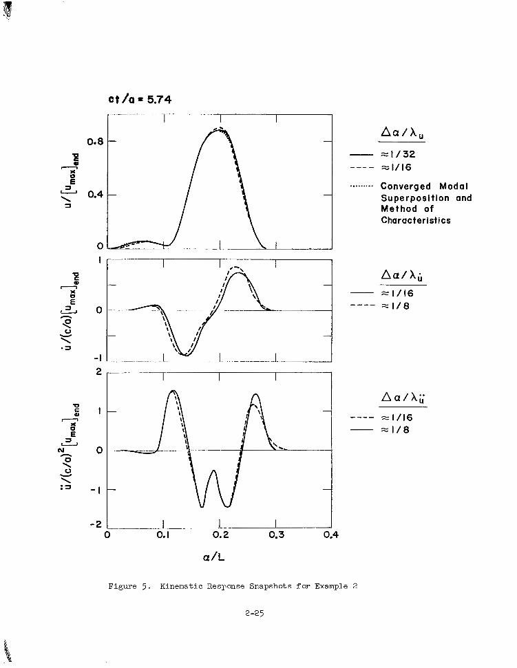
- -1

0.4

2

I

0

- I

- 2

- ." - "I

-

-

I 0. I 0.2 0.3 0.4

a / L

A a / A u

. . . . . . . . . Converged Modal Superposition and Method o f Characteristics

= 1/16 = 1/8 ""

"" = 1/16 = l / 8

Figure 5 . Kinematic Response Snapshots f o r Example 2

2-25

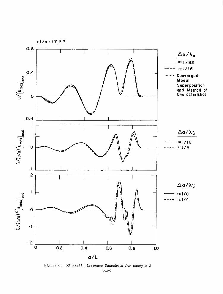
ct /a = 17.22 0.0

0.4

\ o 3

-0.4 L

I I I I Aa/Au 1/32

"" = 1/16

Modal Superposition and Method of Characteristics

.. ...... Converged

I I I Aa/A;

-I I 1 2

I

0

- I

-2

I I I I 1 Aa/A; . - 1/8

=: 1/4 ""

0 0.2 0.4 0.6 0.8 I .o

a / L Figure 6 . Kinematic Response Snapshots for Example 2

2 -26

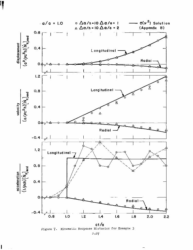
0- 8

0.4

0

1.2

0.8

0.4

0

-0.4

I. 2

0.8

0.4

0

-0.4

a / a = 1.0

1 - ~. ~ 1

Longitudina

A

0.8 1.0 1.2 I .4 1.6 1.8 2.0 2.2

c t /a Figme 7 . Kinematic Respouse Histories for Example 3

2-27

I

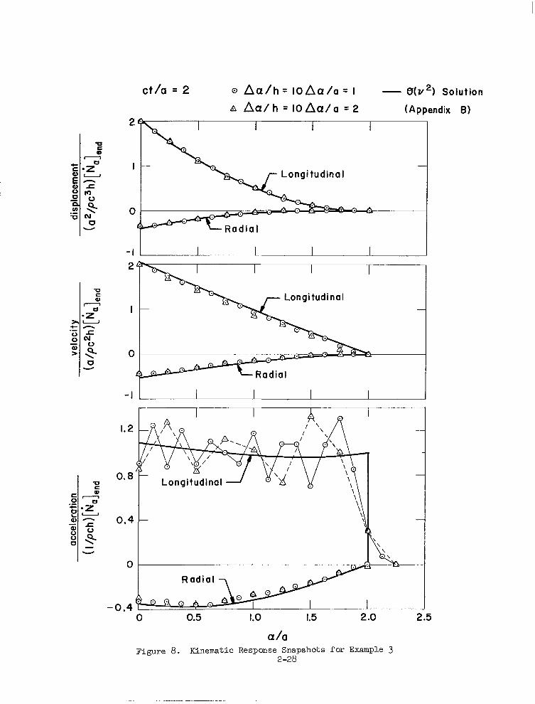
I -

ct/a = 2

2

I

0

- I 2

I

0

- I

I. 2

0.8

-0.4 ""1". .. .

0 0.5 2 .o 1.0 1.5

a /a

2.5

Figure 8 . Kinematic Response Snapshots for Example 3 2 -28

- " - ..........

..........

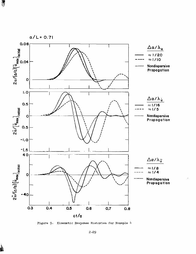
== 1/20 = I / 1.0


== I / I 6 = l / 5


- ""

...- .... = 118 = 1/4


0.3 0.4 0.5 0.6 0.7 0.8

c t/a

Figure 9 . Kinematic Response Hi s to r i e s f o r Example 4

2 -29

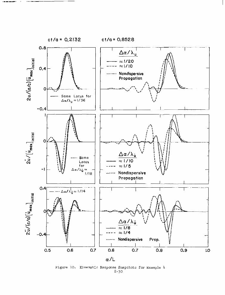
c t / a = 0,2132

Same Locus for

Aa/Xu 1/36

-0.4 I

0

- I

0.4

C

-0.4

ct /a = 0,8528

- = = I / Z O "" = I / ln

.......... Nondispersive Propagation

I I I :: I .. ..


I ' I I I

- 1/8 --- - 1/4 . . .. e . .. .. r Nondispersive Prop. :j' .........

0.5 0.6 0.7 0.6 0.7 0.8 0.9 1.0

a /I- Figure 10. Kinematic Response Snapshots f o r Example 4

2-30

a / L = 0.62

- 0 X

.=! E

I '

0.

1 I I I I I

-

I

C

- I

- 2

-3 0

I -

0-

, I -

-

k'

I I I I I I

I 2 3 4 5 6

c t h

Figure 11. Kinematic Response Histories for Example 5

2 -31

I

c t / a = 1.91 ct /a = 5.73

I I

0 'D I I I

I I

0.5 0.6 0.7 0.8 0.9

........... Nondispersive Propagation and Converged Modal Super- position

A a / h ; - = 1/16

= 1/8


-"- ..........


a / L

Figure 12 . Kinematic Response Snapshots f o r Example 5

2 -32

0.3

0 . 2 c

0. I

0

-0.1

2

I

0

- I

- 2

Figure 13. Kinematic Response Histories for Example 6 2-33

ct /a = 2 A a / h = t o A a / a = I - . . .. . .. .. . . Nondispersive = 1/2 ---- Propagat ion

~

-1""

.- Radial

Longitudinal

2

I

0

- I

- 2

-

0 0.5 1.0 1.5 2.0 2.5 3.0 3.5

a /a Figure 14. Kinematic Response Snapshots f o r Example 6

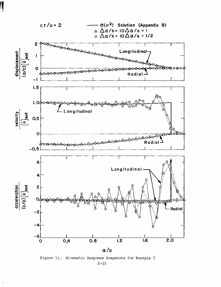
c t / a = 2 - tY(v2) Solution (Appendix B) A Aa/h= loAa/a = I o Aa/h= loAa/a = 112

I

0

- I I I

1.5

h I . 0

g o , 8 Q)

Q) 0.5 > -

-=I

0

-0.5

0 0.4 0.8 1.2 I .6 2 .o

a /a Figure 15 . Kinematic Response Snapshots f o r Example 7

2-35

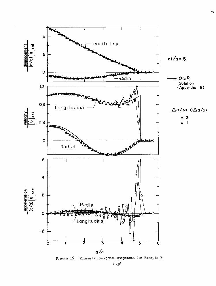
0.4

0

6

4

2

0

-2

ct /a = 5

- Solution

(Appendix B 1

a 2 0 1

Figure 16. Kinematic Response Snapshots f O r Example 7 2 -36

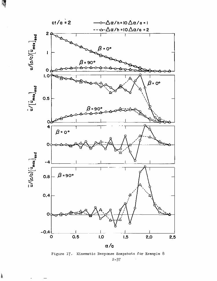
2 '

I

0 , 1.0

0.5

0'

p = oo

4

0

-4

0.8

0.4

0'

- 0.4

I I I

0 0.5 I .o I .5 2.0 2.5

CY /a Figure 17. Kinematic Response Snapshots f o r Example 8

2-37

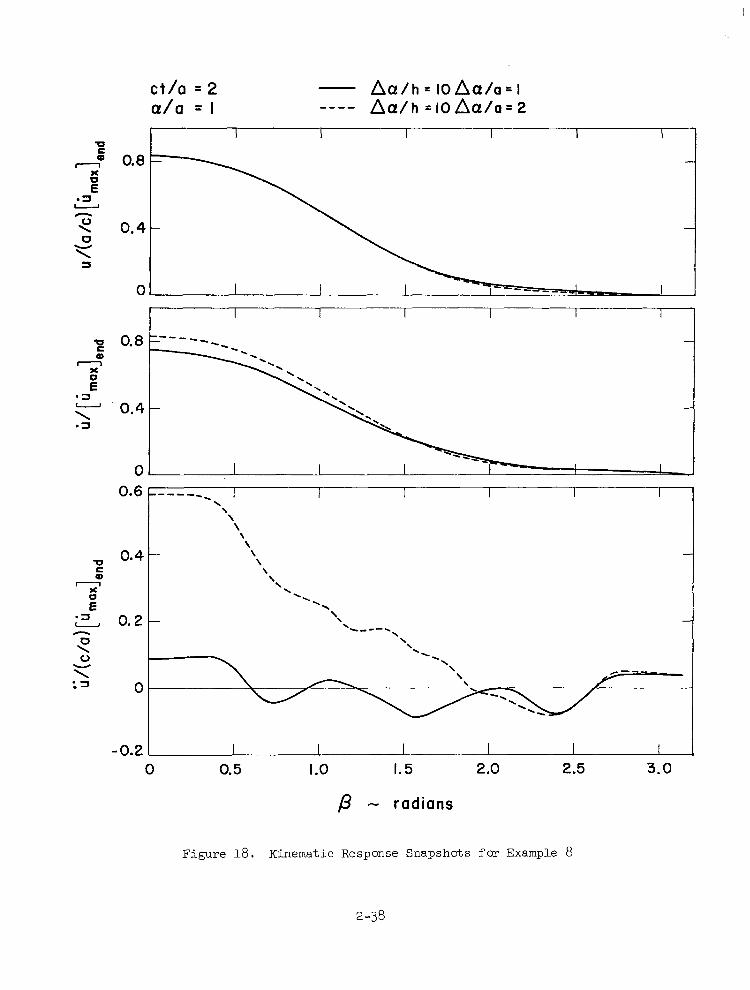
- - 1

n < W 0

\ =I

I I I I I I

0.8 =-" " -

0.4 - -

0 . I I I

I I I I I 0.6 -----_ . \ \ \ \ \ \

0.4 - \ \

- \ \ '. ".

0.2 - \\ - '"". \ '\. -.

\

0

- 0.2 I I 0 0.5 I .o I. 5 2.0 2.5 3.0

p - radians

F i g u r e 18. Kinematic Response Snapshots f o r Example 8

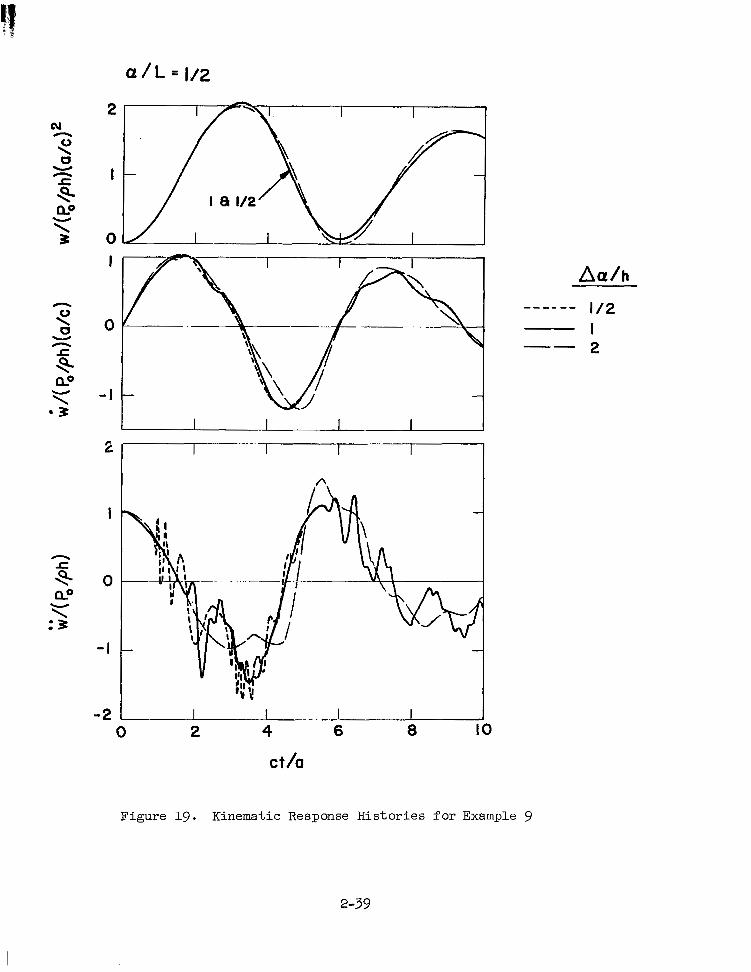
2

I

0 I

0

- I

2

I

0

- I

-2

Aa/h

I12 I 2

"""

"

0 2 4 6 8 IO

ct/a

Figure 19. Kinematic Response Hi s to r i e s f o r Example 9

2-39

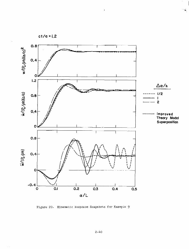
c t / a = 1.2

1.2

0.8

0.4

0 i Aa /h

""" 112 I 2 "

. . .. . . . . . . . . . Improved Theory Modal Superposition

0 0. I 0.2 0.3

a/L 0.4 0.5

Figure 20. Kinematic Response Snapshots f o r Example 9

2-40

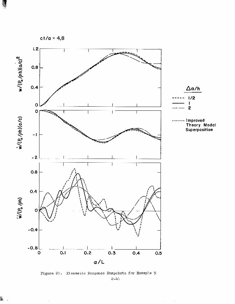
ct /a = 4.8

1.2

0.8

0.4

0

0.8

0.4

0

- 0.4

-0. 8 . L- ! I I 0 0. I 0.2 0.3 0.4 0.5

CY/L

Aa/h

. . . . . . . . . . . Improved Theory Modal Superposition

Figure 21. Kinematic Response Snapshots f o r Examp3.e 9 2-41

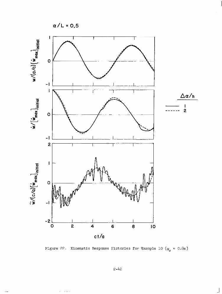
a / L = 0.5

v 0

\ 3

Y :3

- I

I L 0

- I

-2 0 2 4 6 0 10

c t/a

Figure 22. Kinematic Response Histories f o r Example 10 (% = 0.8a)

2 -42

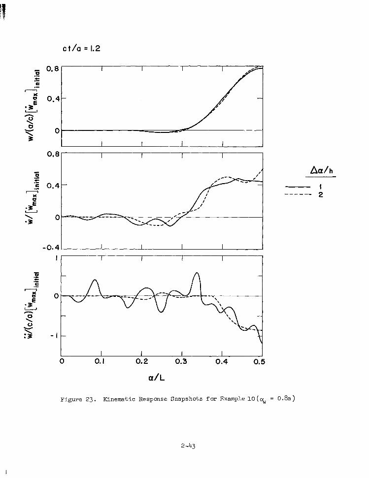
0.8

0.4

0

ct /a = 1.2

-0.4 I I I I I

0

- I

I 2 ””“

1 I I I I 0 0. I 0.2 0.3 0.4 0.5

Figure 2 3 . Kinematic Response Snapshots f o r Example 10 ( s = 0.8a)

2 -43

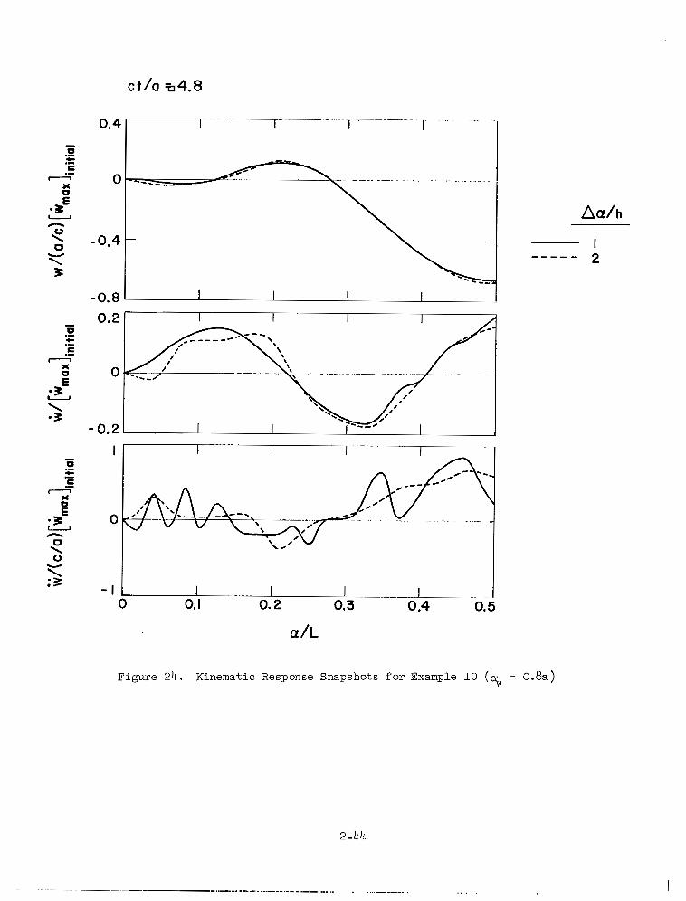
ct/a 4.8

I

0

- I

Figure 24. Kinematic Response Snapshots f o r Example 10 (% = 0.8a)

2 -44

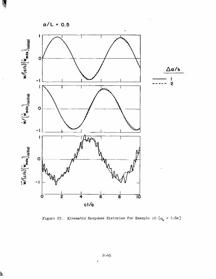
a/L = 0.5

I I I I I I I

- I I

I 2 -”“

I I I I I I

c t/a

0 2 4 6 8 10

Figure 2 5 . Kinematic Response Histories f o r Example 10 (s = 1.6a )

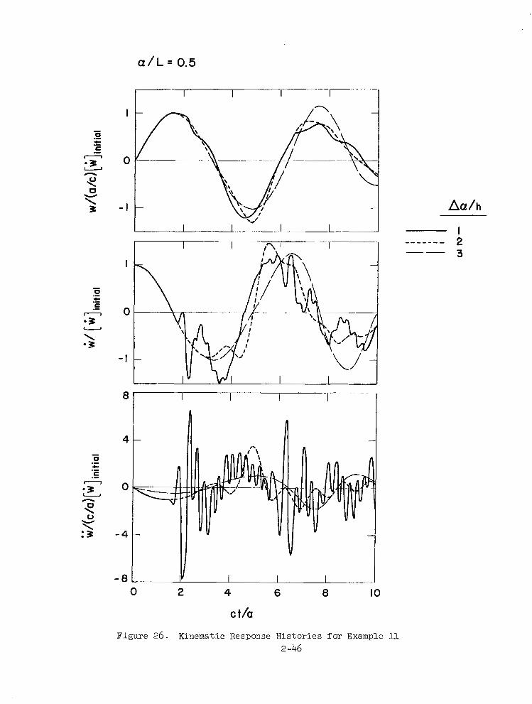
a / L = 0.5

I

0

- I

I

0

- I

8

4

0

- 4

- 8 0 2 4 6 8 IO

c t/a

Figure 26. Kinematic Response Histories f o r Example 11 2 -46

I 2 3

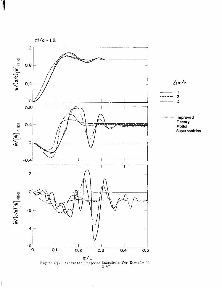
1.2

0.8

0.4

0 0.8

Ob 4

0

-0.4

2

0

-2

-4

-6

I " ~ I' I I

-

*- - . . . .

. . . . . . . : .:

0 0. I 0.2 0.3 0.4 0.5

a/L Figure 27. Kinematic Response Snapshots f o r Example 11

2 -47

Aa/h

............ Improved Theory Modal Superposition

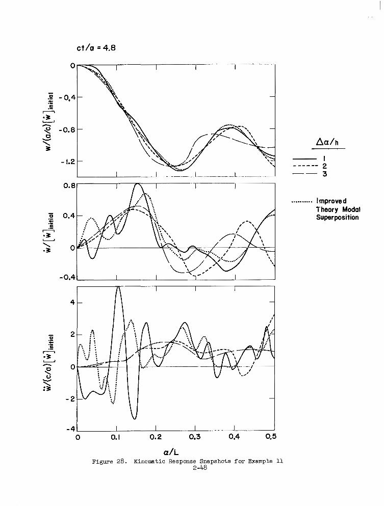
ct/a =4.8

-5 I

- 1.2 <\ L

.......... Improved Theory Modal Superposition

- 4 Y - 0 0. I 0.2 0.3 0.4

a/L Figure 28. Kinematic Response Snapshots f o r Example 11

2 -48

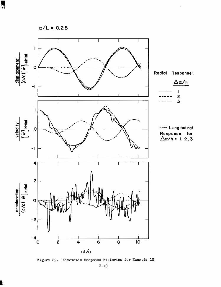
a / L = 0.25

0

- I

2

0

-2

I I I I I 0 2 4 .6 8 IO

ct /a

Figure 29. Kinematic Response Histories for Example 12

2 -49

Radial Response :

Aa/h

I 2 3

"" - "

. . . . . . . . Longitudinal

Response for h / h = I, 2,s

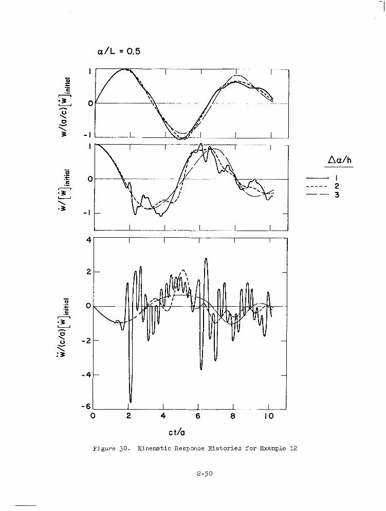
a / L = 0.5

I

0

- I I

0

- I

4

2

0

-2

- 4

-6 0 2 4 6 8 I O

c t/a

Aa/h

I 2 3

""e

"

Figure 30. Kinematic Response Histor ies for Example 12

2-50

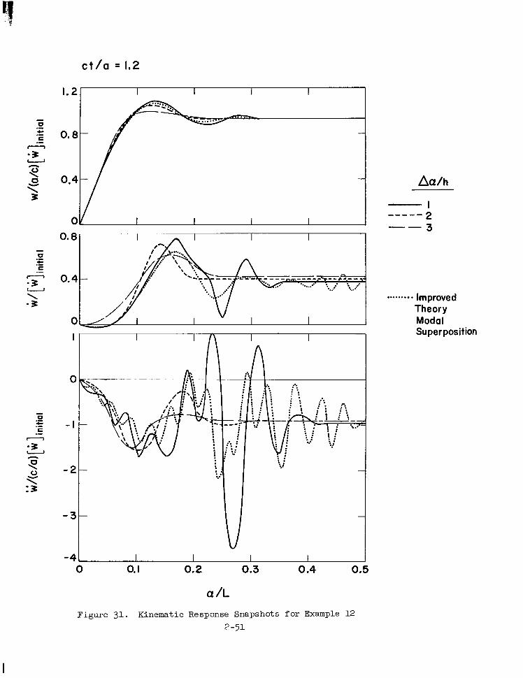
c t / a = 1.2

1.21 I I I I

I

C

- I

- 2

- 3

-4 0 0. I 0.2 0.3 0.4 0.5

a /L

A a / h

I 2 3

""- "

. . . . . . . . . Improved Theory Modal Superposition


2 -51

I

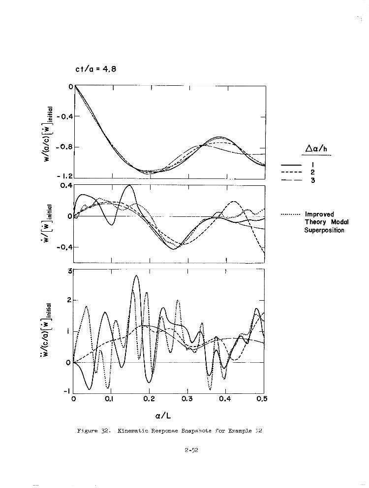
c t / a = 4.8

.- - A a / h

I 2 3

""_ "

. . . . . . . . . . Improved Theory Modal Superposition

-3 \ \

-0.4- \- \

31 I I I I I

0 0. I 0.2 0.3 0.4 0.5

a/L


2 -52

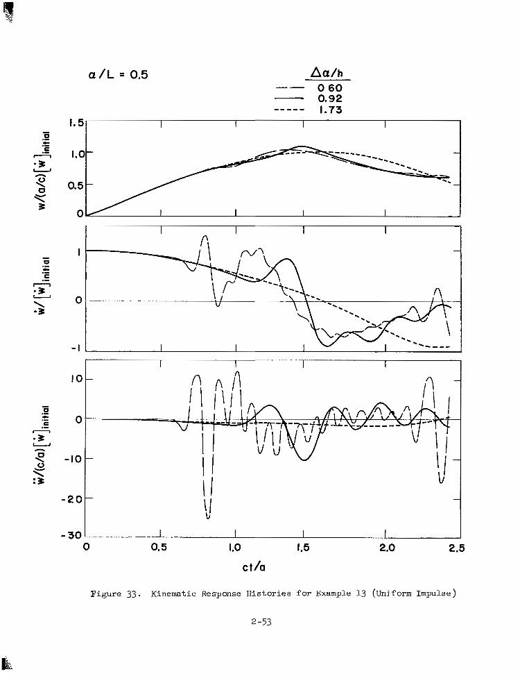
a / L = 0.5 Aa/h " 0 60

0.92 I .73 " "-

1.5 I I I I

1.0-

0 0.5 1.0 1.5 2.0 2.5

ct/a

Figure 33. Kinemat ic Response His tor ies for Example 13 (Uniform Impulse)

2 -53

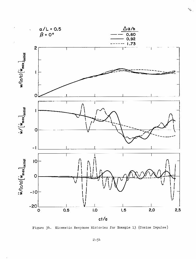
.. a / L = 0.5 Aa/h 0.60 0.92

I .73

p = oo "

"""

2 I - 1 -~ ~~~ ~

-

' t /" - ----"""- =- I -

0 I I ~~ .~ ~ -1 . ~ -~ . .

- I I I

0 0.5 I .o I. 5 2.5

ct/a

Figure 34. Kinematic Response Histories for Example 13 (Cosine Impulse)

a / L = 0.5 p = 90"

Aa/h 0.60 0.92 1.73

"

""_

I

0

- I

- 2

0

I I I I

I I I V 0.5 I .o

c t /a

1.5 2 .o 2.5

Figure 35. Kinematic Response Histories f o r Example 13 (Cosine Impulse )

2-55

I

ct/a = 0.70 Q/L = 0.5

n u /h " 0.60

. 0.92 & 1.73

~~

I I 1

p - degrees

Figure 36. Kinematic Response Snapshots for Example 13 (Cosine Impulse )

2-56

ct/a = 0.78 Aa/h " 0.60

0.9 2 1.73 ""_

I

" ---

0 I

- I I O

5

0

5

-I 0 0 0. I 0.2 0.3

a / L 0.4 0.5

Figme 37. Kinematic Response Snapshots f o r Example 13 (Uniform Impulse)

. . .. . . . . . . . . . . . .. -

" I

ct/a = 0.78 p =oo

Aa/h " OI60

0.9 2 I .73 """

I

0

- I I .O

Y :3 -0.5

-1.0

I I I I

0 0. I 0.2 0.3 0.4

Q /L

Figure 38. Kinematic Response Snapshots for Example 13 (Cosine Impulse )

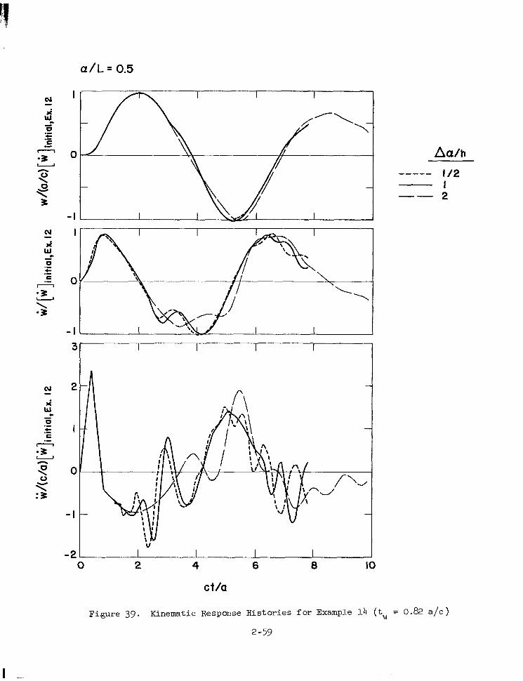
a / L = 0.5

0 2 4 6 0 IO

c t/a

""_ I /2 I 2 "

I

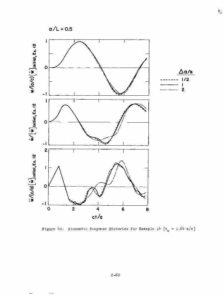
a / L = 0.5

I I I I I I

0 2 4 6 0

c t /a

Aa/h 112 I 2

"""-

"

Figure 40. Kinematic Response Histories for Example 14 (tw = 1.64 a/.)

2 -60

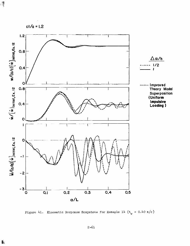
ct/a = 1.2

I I

...............

I

Aa/h ""- 112

i I

......... ImProved p! 0.8 I I I Theory Modal x Superposition - (Uniform c Impulsive .- Loading 1

w 0 "

.- *E 0.4 -

a 3

\

- - *B 0

I __"-r-- I

c E .- .- - - I - I n

0 K :L -2-

-3 I I 0 0.1 0.2 0.3 0.4 0.5

a/L

Figure 41. Kinematic Response Snapshots f o r Example 14 (t, = 0.40 a/.)

2 -61

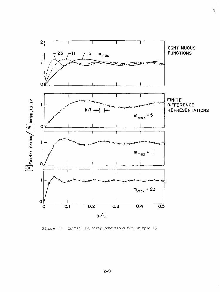
I I I I I I

I J I

I I I I I I

Ob( I I I I I

max = 23

0 0. I 0.2 0.3 0.4 0.5

a/L

Figure 42. I n i t i a l Ve loc i ty Condi t ions for Example 1 5

CONTINUOUS FUNCTIONS

FINITE DIFFERENCE REPRESENTATIONS

2 -62

a / L = 0.5

0 2 4 6 0 I O

ct /a

Figure 43. Kinematic Response Histories f o r Example 15 (mmax = 5 )

2 -63

a / L = 0.5

0 2 4 6 0 IO

""_ 1/2 I 2 "

c t/a

Figure 44. Kinematic Response HTstories fo r Example 15 (mmax = 11)

2 -64

a / L = 0.5

I

0

- I

I I 1

2

0

-2

A

V

I I I I I I

0 2 4 6 8 10 I

Aa/h

ct /a

Figure 45. Kinematic Response Histories for Example 1 5 (m max = 2 3 )

2-65

Longitudinal Stress: I

I Aa/A, a/L = 0-24 == 1/16 = 118 " ""

0 . . . . . . . . . . . . Improved Theory Modal Superposition

- I I I . ..

0 4 0 12 16 " Circumferential

ct/a Stress

0 1 e 0 .

0

I 0 I I

c t / a = 5.73

L"

I 0. I 0.2 0.3

c t / a = 17.2

0 /

- I 1 I I I 1

0 0.2 0.4 0.6 0.8 1.0

a / L

Figure 46. S t r e s s Response History and Snapshots f o r Example 2

2 -66

a / a = 1.0 0

- u ( v * ) Solution

Circumferential (Appendix 6)

Aa/h = IOAa/a= 0 1

-0.8 0 2

- 0.4

0 c - 0 - 1.2 U -2

0 1.0 1.5 2.0

w I- v)

"

a 0

- I

- 2

ct/a

c t / a = 2.0

Circumferential

0.5 1.0 1.5 2.0

a /a

-" - Method of Characteristics ( M;re;;ane )

Figure 47. S t r e s s Response History and Snapshot for Example 3

2 -67

I

0

- I

a/L = 0.62

cu

0

- I

c t /a 1.91

2 4 6 c t/a

.......... Improved Theory Modal Superposltion

ct/a = 5.73

0.6 0.7 0.5 0.6 0.7 0.8 0.9

a / L

Figure 48. S t r e s s Response History and Snapshots for Example 5

2 -68

A 0 . 5 0 1 0 2

0.4 r I I I I I

I ct /a = 2.0

0.4

in

0

-0.4

I I I I I

- 1.2 I I I I

0 I 2 3 4 5

b

a /a Figure 49. S t r e s s Response Snapshots f o r Example 7

2 -69

ct /a = 2.0 0 A a / h = l o A a / a = I A A a / h = 10 A d a = 2

Circumferential

1 0 0.4 0.8 1.2 I .6 2 .o 2.4 2.8 3.2

p - radians 0.4

01

- 0.4

- 0.8

I . 2‘

I Cirmmferential

I I I

q . ’. \ “d .

I I I

0.8

,- Longitudinal

p = 9 0 ° -

1

-0.4 I 0 0.4 0.8 1.2 I .6 2.0 2.4

I . ~. ~~ -..I I . -”

a /a Figure 50. S t r e s s Response Snapshots fo r Example 8

2 -70

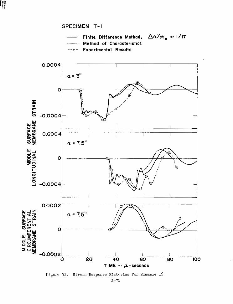
SPECIMEN T- I

- Finite Difference Method, A a l c t , = 1/17 ..... - ..... Method of Characteristics

-0- Experimental Results

0.0004 ~

I I

= 3"

0.0004

0

-0.0004

0.000 2

0

-0.0002 0

CY = 7.5"

20 40 60 80 100 T IME - p- seconds

F i g u r e 51. Strain Response Histories f o r Example 16 2 -71

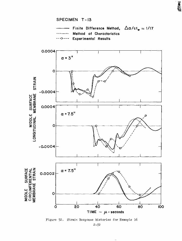
SPECIMEN T - I3

0.0004

0

-0.0004

Fini te Di f ference Method, Aa/ct , == 1/17 Method of Characteristics . . . . . . . .. . . . . .

" Q" - Experimental Results

0.00 0 4

0

-0-0004

I I l

a = 3"

a = 7.5" P

I I

I I

a = 7.5" 0.0002 -

0 .

I I 0 20 40 60 80 100

TIME - p - seconds

Figure 52. St ra in Response H i s to r i e s fo r Example 16 2 -72

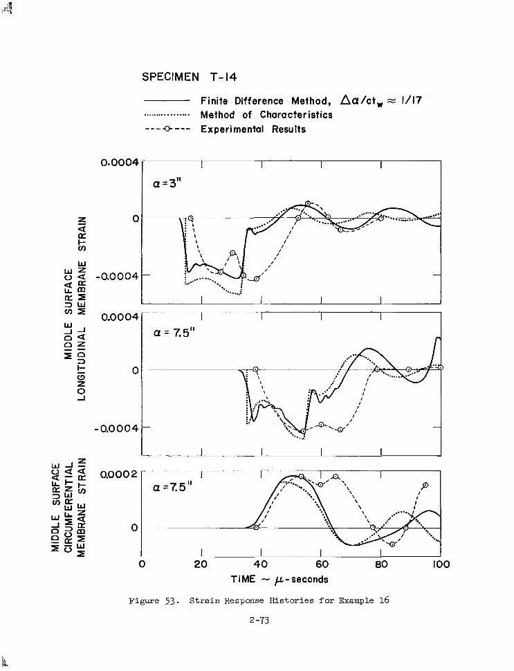
SPECIMEN T- 14

0.0004

w z w

o a -0.0004

a s 3 w * $ E

0.0004

Finite Difference Method, A a / c t , = 1/17 .............. ". Method of Characteristics -"e"- Experimental Results

-0.0004

I I I I

a = 3"

0 20 40 60 80 too TIME - p- seconds

Figure 53. S t r a i n Response Histories f o r Example 16

2 -73

I , , ."

E x p e r i m e n t a l

a. "- - Finite Difference, h / h = I

701

0 IO 20 30 40 5 0 60 70 80

7 0

60

5 0

40

30

IO

0

I

IO 20 30 40 5 0 60 70 80

121 I I I I I 1

- 2 0 10 20 30 40 50 60

Z U

0

-20

20

0

- 20 0 20 40 60 80 100 120

T I ME - p - seconds

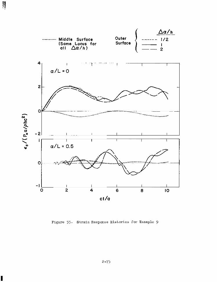
4

2

0 n cu 0 c

0 &O -2

...- .......... Middle Surface (Same Locus for a l l Aa/h )

Aa/h I /2 I 2

Outer Surface

- ""_ - "

. .... "" ... - . " U . 9 ~-~ --.. .......... ........... "...... ........... ........... .......................... .....................

U

\ I I I I I I U

W a / L = 0.5

- I I I I I I 0 2 4 6 8 IO

ct/a

Figure 55. Strain Response Histories for Example 9

2 -75

2

I

0

. . . .. . . . . . . . . . . . . . . Middle Surface (Same Locus for

0 1 1 h / h )

Aa/h Outer """ 112 Surface I

2 "

ct/a = 1.2

ao W

\ c t/a = 4.0 w U

I

I

0

- 1 __

cu n

= - I 0 2 1 I I I ~ I ~ ~ . " ~ ~. . ~ _.

0 0. I 0.2 0.3 0.4 0.5

a / L

Figure 56. S t ra in Response Snapshots fo r Example 9

............. Aa/h

1/2 Middle Surface (Same Locus for Surface I all Aa/h) " 2

Outer -.- - - - -

0.4 I 1 I I I I

a/L=0.5 - 0.4 I I I I I I

0 2 4 6 8 10

ct /a

0.4 I I /

............... 0" v - - . . >*..? ......... " ...............

"

-0.4 mz 0.4 I 7- -~ ~ -1 I

.................... ct/a =4.8 - 0.4 _ - ~ _ _ _ 1.- . I I I -

0 0. I o. 2 0.3 0 A 0.5

Cf/L

Figure 57. S t r a i n Response History and Snapshots for Example 10 (% = 0.8a)

Modal Superposition -") Outer

Aa/h= I - Surf ace .... - .... Middle Surface for = 2 ""_ all Cases

I

0

- I

0 __ ""I. ., - "1"

2 4 6 8 IO c t/a

I c c t /a = 4.8 /

0

2

I

0

- I

-2 2

I

0

- I

-2 3

2

I

0

-I

a / L = 0.5

. . . . . . . . .. . . . Middle Surface (Same Locus for all Aa/h)

h / h

O u t e r ""-" 0.60 Surface 0.92

1.73 "

Uniform -

I I I

I I I I

Cosine Impulse - p = o *

-

c t/a

Figure 59. S t r a i n Response Histories f o r Example 13

2 -79

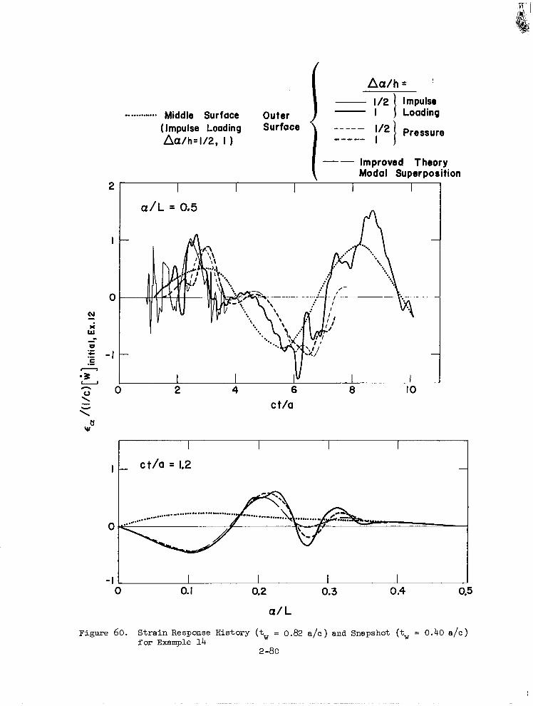
.. ...... ”... Middle Surface Outer (Impulse Loading Surface Aa/h=1/2, I 1

I

Aa/h = !

l - I Loading ””_

112 1 Pressure I ””- I

” Improved Theory Modal Superposition

I

0

-I

0 2 4 6 8 IO c t/a

c I

I c t /a = 1.2 I - I 1 ~ . -1 0 0. I 0.2 0.3 0.4 0.5

a/ L

Figure 60. S t r a i n Response History (t, = 0.82 a/.) and Snapshot (t, = 0.40 a/.) f o r Example 14

2 -80

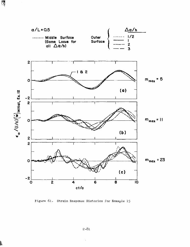
a / L = 0.5 Aa/h ...,...... * Middle Surface Outer ""_ - I /2

I 2 3

(Same Locus for Surf ace all Aa/h)

- """

"

max = 23

Figure 61. Strain Response Histories for Example 1 5

2 -81

Chapter 3

ANALYTICAL STUDY OF CONVERGENCE

The primary objective of t h i s chap te r i s to s tudy the causes of the con-

vergence problems encountered i n Chapter 2 . Two causes are possible: limi-

ta t ions i nhe ren t i n t he f i n i t e d i f f e rence me thd , and l imi t a t ions of the

she l l t heo ry employed.

It i s c l e a r t h a t i n problems characterized by the presence of response

discont inui t ies , there a lways exis ts a region near each discontinuity where

non-convergent osc i l la t ions in the f in i te d i f fe rence computa t ions occur .

Even though this behavior causes only marginal d i f f icul t ies , it s t i l l re-

presents an inherent l imitat ion of t he f i n i t e d i f f e rence method.

We observed i n Chapter 2 Convergence problems r e l a t e d t o f l e x u r a l r e -

sponse computations that are not caused by the presence of d i scon t inu i t i e s

in the response of i n t e r e s t . We w i l l s e e i n t h i s c h a p t e r t h a t t h i s d i f f i c u l t y

i s no t t he r e su l t of a l i m i t a t i o n i n t h e f i n i t e d i f f e r e n c e method i t s e l f ,

b u t i s ins tead the resu l t of a l imi t a t ion of the th in she l l (Bernoul l i -Euler )

theory used.

There i s ample ev idence in the resu l t s of Chapter 2 t h a t t h e convergence

d i f f i c u l t i e s of f ini te difference computat ions are associated with response

components wi th shor t s t ruc tura l wave lengths . For these components, s h e l l

curvature effects are unimportant and it i s t h e r e f o r e j u s t i f i a b l e t o con-

sider the simpler case of a p la te ins tead of a shell. Furthermore, since

convergence d i f f icu l t ies in the absence of response discont inui t ies have not

occurred for shel ls subjected to in-plane exci ta t ions, we need only consider

transverse motions o f t he p l a t e .

The p r inc ipa l r e su l t s of t h i s Chapter are (1) tha t t he f i n i t e d i f f e rence

method f a i l s t o converge only in r eg ions around d iscont inui t ies in the response

of i n t e r e s t , ( 2 ) that f lexural response convergence problems not i n r eg ions

around response discont inui t ies are the direct resul t of t h e f a i l u r e of t h i n

shel l (Bernoul l i -Euler) theory, and (3) t h a t a t h i n s h e l l f i n i t e d i f f e r e n c e

so lu t ion may be more accurate than even an exact solution of the corresponding

d i f fe ren t ia l equa t ions . In addi t ion , it i s pointed out that the method of

3-1

mcdal supe rpos i t i on a l so suffers from convergence limitations, and t h a t t h e

use of improved s h e l l (Timoshenko) theory ins tead of t h i n s h e l l t h e o r y w i l l

tend t o r e l i e v e sane of t he convergence d i f f i c u l t i e s a s s o c i a t e d w i t h com-

putat ions of flexural response, but may a l s o prove t o be inadequate for

some purposes.

3 .1 CONVERGENCE OF FINITE DIFFERENCE COMPUTATIONS OF FLEXURAL RESPONSE

This sect ion examines the dynamic c h a r a c t e r i s t i c s of a f in i t e d i f f e rence

model of a t h i n p l a t e . These charac te r i s t ics a re then re la ted to those of

the continuous plate and convergence of t h e f i n i t e d i f f e r e n c e model i n t h e

l i m i t of vanishing mesh s i z e i s demonstrated.

3.1.1 Frequency Equation for the F in i te Di f fe rence P la te

A convenient way to cha rac t e r i ze t he dynamic behavior of a system

i s t o determine the frequency equation for the system. Such an equation

relates the (angular) f requency U) t o t h e wave number k. A s shown i n t h e

subsequent derivation for a p l a t e , and as R e f . 19 shows f o r simple discrete

systems, the frequency equation cv = w(k) f o r homogeneous d i s c r e t e systems

i s independent of t he boundary conditions and the number of degrees-&-freedom;

d i f f e ren t boundary conditions or a d i f f e r e n t number of degrees-of-freedom

merely give different points on the same U) = w(k) curve. It should a l s o

be noted that the frequency equation i s the same f o r t r a v e l i n g waves, stand-

ing waves due t o free osc i l l a t ions , and forced s inusoida l osc i l la t ions

(Ref. 19) ; again the different cases s imply give different points on the same

frequency curve U) = ~ ) ( k ) . The frequency equation w i l l now be determined for the d i scre te sys tem

t h a t r e s u l t s from a f in i t e d i f f e rence r ep resen ta t ion of t h e f l e x u r a l motion

of a t h i n , f l a t p l a t e . A comparison i s then made between the frequency

equat ion for the cont inuous plate and that f o r t h e f i n i t e d i f f e r e n c e p l a t e

i n t h e limit of vanishing mesh width.

3 -2

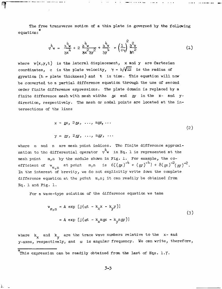
IT - """."_... .. ...._. ." . . . .. ..... . . -. . . ......

The f r ee t r ansve r se motion of a t h i n p l a t e i s governed b y t h e f o l l m i n g * equation:

where w(x,y,t) i s the la te ra l displacement, x and y are Cartesian

coordinates, c i s the p l a t e ve loc i ty , y = h / f i i s the r ad ius of

gyration (h = pla te th ickness) and t i s time. This equation w i l l now

be converted t o a par t ia l d i f ference equat ion through the use of second

o rde r f i n i t e d i f f e rence expres s ions . The p l a t e domain i s replaced by a

f i n i t e d i f f e r e n c e mesh w i t h mesh widths p and i n t h e x- and y-

d i rec t ion , respec t ive ly . The mesh or noda l po in t s a r e l oca t ed a t t he i n -

t e r sec t ions of t he l i nes

X = &x, 2&, . . ., mhx, . . .

y = u, 2 ~ , . . ., n u , . . . where m and n a re mesh poin t ind ices . The f in i te d i f fe rence approxi -

mation t o t h e d i f f e r e n t i a l o p e r a t o r v w i n Eq. 1 i s represented a t t h e

mesh point m,n by the module shown i n F i g . 1. For example, the co-

e f f i c i e n t of w a t p o i n t m,n i s 6 [ AX)-^ + ( ~ ) - ~ l + 8( F ) - ~ ( D ) - ~ . I n t h e i n t e r e s t of brev i ty , we do not expl ic i t ly wri te down the complete

d i f fe rence equat ion a t the po in t m,n; it can readily be obtained from

Eq. 1 and Fig . 1.

4

m, n

For a wave-type so lu t ion of the difference equation we take

W = A exp [ j ( w t - kxx - kyy)1 m, n

= A exp [ j ((ut - kxmD - kynN) l

where kx and k a re t he t r ace wave nunibers r e l a t i v e t o t h e x- and

y-axes, respectively, and u) i s angular frequency. We can write, therefore , Y

* This expression can be readi ly obtained f rm t h e l a s t of Eqs. 1.7.

3-3

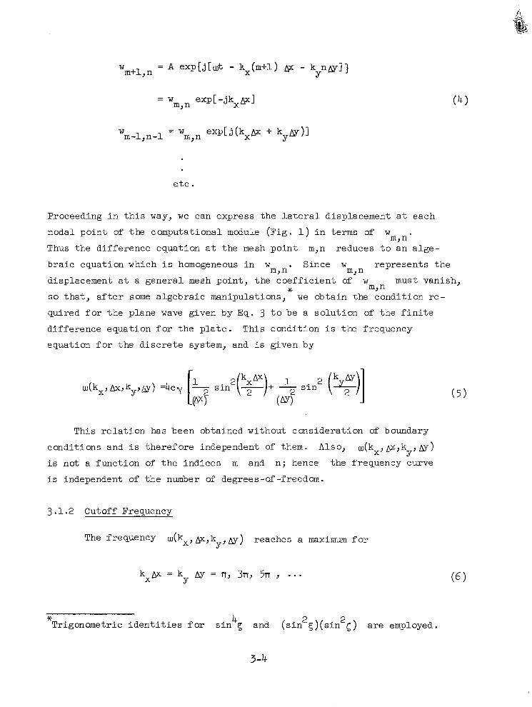
W = A exp{j[wt - kx(m+l) @ - k y n ~ ] ] m+l , n

= w exp[- jkxp] m, n

e t c .

Proceeding i n t h i s way, we can express the la teral d isplacement a t each

nodal point of the computational module (Fig. 1) i n terms of w . Thus the d i f fe rence equat ion a t the mesh poin t m,n reduces t o an a lge-

braic equat ion which i s homogeneous i n w . Since w represents the

displacement a t a general mesh poin t , the coef f ic ien t of w must vanish,

so t h a t , a f t e r some algebraic manipulations, we obtain the condition re-

qu i red for the p lane wave given by Eq. 3 t o be a so lu t ion of t h e f i n i t e

difference equation f o r the plate . This condi t ion i s the frequency

equa t ion fo r t he d i sc re t e system, and i s given by

m, n

m, n m, n

* m, n

This relation has been obtained without consideration of boundary

conditions and i s therefore independent of them. Also, w ( k x , g J k y J D )

i s not a funct ion of the ind ices m and n; hence the frequency curve

i s independent of the number of degrees-of -freedom.

3.1.2 Cutoff Frequency

The frequency dkx, @,ky, m ) reaches a maximum f o r

* 4 2 2 Trigonometr ic ident i t ies f o r s i n 5 and ( s i n S ) ( s i n c ) a r e employed.

3-4

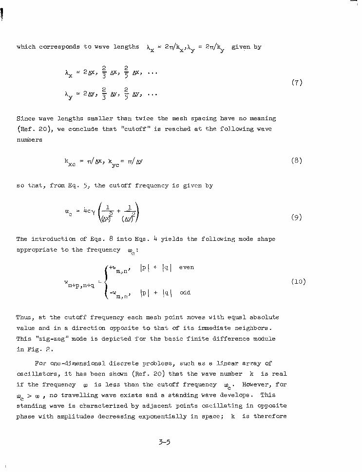
which corresponds t o wave lengths Ax = 2n/kx,Ay = 2n/ky given by

Since wave lengths smaller than twice the mesh spacing have no meaning

( R e f . 20) , we conclude that "cutoff 'I i s reached a t t h e f o l l o w i n g wave

numbers

s o t h a t , from Eq. 5 , the cutoff frequency i s given by

The introduct ion of Eqs. 8 i n t o Eqs. 4 yields the fol lowing mode shape

appropriate to the f requency wc:

Thus, a t the cutoff f requency each mesh poin t moves with equal absolute

value and i n a direct ion opposi te t o t h a t of i t s immediate neighbors.

This "zig-zag" mode i s dep ic t ed fo r t he bas i c f i n i t e d i f f e rence module

i n F i g . 2 .

For one-dimensional d i s c r e t e problems, such a s a l i nea r a r r ay of

o sc i l l a to r s , it has been shwn (Ref. 20) t h a t t h e wave number k i s r e a l

i f the f requency w i s less than the cutoff frequency wc. However, f o r

> w , no t rave l l ing wave e x i s t s and a standing wave develops. T h i s

standing wave i s charac te r ized by ad jacent po in ts osc i l la t ing in oppos i te

phase with amplitudes decreasing exponentially in space; k i s therefore

3-5

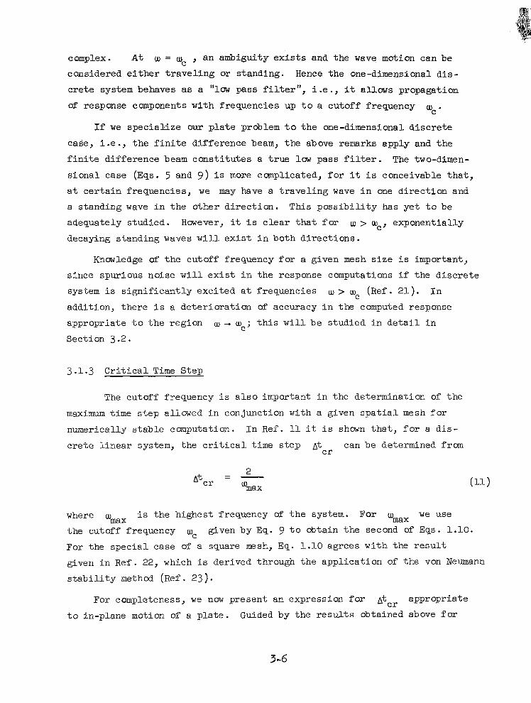
complex. A t 01 = w an ambigui ty exis ts and the wave motion can be

considered either t r a v e l i n g or standing. Hence the one-dimensional d i s -

crete system behaves as a "low pass filter", i .e ., it allows propagation

of response components with frequencies up t o a cutoff frequency 01 .

c '

C

If we spec ia l ize our p l a t e problem t o t h e one-dimensional discrete

case, i .e . , the f i n i t e d i f f e r e n c e beam, the above remarks apply and the

f i n i t e d i f f e r e n c e beam cons t i t u t e s a t r u e low p a s s f i l t e r . The two-dimen-

sional case (Eqs. 5 and 9 ) i s more complicated, for it i s conceivable that ,

a t c e r t a i n f r e q u e n c i e s , w e may have a t r ave l ing wave i n one d i r ec t ion and

a s tanding wave i n the o ther d i rec t ion . Th i s p o s s i b i l i t y h a s y e t t o b e

adequately studied. However, it i s c l e a r t h a t f o r I,U > uc, exponent ia l ly

decaying standing waves w i l l e x i s t i n b o t h d i r e c t i o n s .

Knowledge of the cu tof f f requency for a given mesh s i z e i s important,

since spurious noise w i l l exis t in the response computat ions i f t he d i sc re t e

system i s s ign i f i can t ly exc i t ed a t f r equenc ie s w > wc (Ref. 21) . I n

addi t ion, there i s a d e t e r i o r a t i m of accu racy i n t he computed response

appropriate t o t h e r e g i o n w + w - th i s w i l l b e s t u d i e d i n d e t a i l i n

Section 3.2. C '

3.1.3 C r i t i c a l Time S tep

The cutoff frequency i s a l so impor tan t in the de te rmina t ion of the

maximum time step allowed in conjunction wi th a g iven spa t i a l mesh for

numerically stable computation. In Ref. 11 it i s shown t h a t , f o r a d i s -

c r e t e l i n e a r system, the c r i t i c a l time s t e p A t can be determined from c r

where %x i s the highest frequency of the system. For wmx we use

the cutoff frequency wc given by E q . 9 t o obtain the second of Eqs. 1.10.

For the special case of a square msh, E q . 1.10 agrees wi th the r e s u l t

given in Re f . 22, which i s der ived through the appl icat ion of the von Neumann

s t a b i l i t y method ( R e f . 23) .

For completeness, w e now present an expression for A t c r appropriate

t o in-plane motion of a p l a t e . Guided by the resul ts obtained above f o r

3-6

t ransverse motion, we assume t h a t the cutoff frequency corresponds t o a zig-zag mode fo r ad j acen t mesh points (Fig. 2) . Then, from the governing

difference equations for in-plane motion, or through the application of

Rayleigh's principle, w e can readi ly show t h a t

where c = [E/2(l+v)p]1/2 i s the shea r ve loc i ty . In t roduc ing t h i s i n to

Eq. 11, w e obtain the f i r s t of Eqs. 1.10; t h i s r e s u l t a g r e e s w i t h the

r e s u l t of R e f . 24, which a l s o employs the von Neumann s t a b i l i t y c r i t e r i o n .

N a r it has been stated (Ref. 25) that E q . 11 i s inconvenient in appl ica-

t ion because of t h e d i f f i c u l t y of determining wmax; we have ju s t s een t ha t

the assumption of zig-zag motion constitutes a very simple means for over -

coming t h i s d i f f i c u l t y .

S

3.1.4 Convergence of the F in i te Di f fe rence Method . ~~ . . "

Eq. 5 i s the f requency equat ion for the f ini te difference plate .

We now consider the l imit ing case when the mesh widths p$ and w both approach zero. Thus we have, f o r f i x e d s t r u c t u r a l wave numbers

and k kX

Y)

so that the Taylor ' s se r ies expans ion for s in f then yields

This i s i n agreement with the frequency equation for the uniform plate,

which may be obtained from R e f . 26. Thus, a f i n i t e d i f f e r e n c e s o l u t i o n does, i n f a c t , converge t o the corresponding continuous solution as

w , &f 0 , i n t h e absence of response discont inui t ies .

3-7

3.2 FFEQUENCY PARAMETERS

I n this sect ion, w e g ive express ions for the charac te r i s t ic f requency

pa rame te r s t ha t pe r t a in t o t he she l l t heo ry employed, the given exci ta t ion?

and t h e f i n i t e d i f f e r e n c e mesh. These parameters are then used t o i n t e r -

p r e t some of the numerical results presented in Sec t ion 2 . A f i n i t e d i f f e r -

ence computational procedure based on the use of these parameters i s then

presented.

3 .2 .1 L i m i t Frequencies of S h e l l Theory

Thin she l l t heo ry i s l imi ted to the f requency range (Ref . 7 )

f o r f l e x u r a l motion, and

w 2 w =ws e

for extensional motion. In these equat ions, i s the frequency of

the lowest antisymmetric thickness-shear mode of a plate , g iven by wS

For comparison, we a l s o w r i t e t h e limit frequency appropr ia te to

improved theory (Ref. 7 )

We observe t h a t we= wi = 10 Wf .

3.2.2 Cutoff Frequency of Exci ta t ion

A convenient way t o describe a t r ans i en t exc i t a t ion i s t o char-

a c t e r i z e it i n terms of i t s frequency content, through the use of the

Fourier transform (Ref. 2 ) . For example l e t us consider a funct ion

3-8

with the f olluwing tr iangular temporal variation (Fig. 3 )

, 0 r ; t s - t 1 2 w I Lw

, "t s t s t w 1 2 w

\ O , otherwise

The Fourier transform of f (t ) is then (Eq. 1 . 2 )

Figure 3 shows the spectrum - ~?(IJ)I from Eq. 20. This spectrum i s

c l e a r l y a compact funct ion with a reasonably wel l def ined exci ta t ion

cutoff frequency given by

2

tW

4rr wx M - tW

Not a l l e x c i t a t i o n s a r e b l e s s e d w i t h a wel l def ined exci ta t ion

cutoff frequency. It i s of ten desirable t o f i l t e r such exc i t a t ions

in o rder to enforce cu tof f . This w i l l be discussed shortly in Sub-section

3.2.5.

3.2.3- L i m i t Frequency of Mesh

We have observed in the p rev ious sec t ion tha t harmonic waves wi th

frequencies greater than the cutoff frequency w i l l not propagate in the

f in i t e d i f f e rence ana log of a continuous system. Furthermore, there i s

no guarantee that the discrete system w i l l accurately represent all waves

propagating in the continuous system with w < wC. The degree of inaccuracy

i s , in fac t , ind ica ted by the d ivergence between the frequency equations

3-9

f o r t h e two systems. Let us nm def ine a l imit f requency of the mesh

( W ) below which the f requency curve for the discrete system diverges

by less than a prescr ibed amount from the f requency curve for the con-

tinuous system. That is, l e t % be the highest value of u) f o r which

the fo l lowing re la t ionship ho lds :

m

where the numerator of t he f r ac t ion i s given by Eq. 5, the demoninator

i s the f requency equat ion for the cont inuous plate , and E <.= 1. Now we

might use any one of three frequency equations for the continuous plate:

tha t appropr ia te to e lementary (Bernoul l i -Euler ) theory, that appropriate

t o improved (Timoshenko) theory and, f i n a l l y , t h a t a p p r o p r i a t e t o e l a s -

t i c i t y t h e o r y . If we take the shear constant of impraved t h e o r y e q u a l t o

m /12 , t h e l a t t e r two frequency equations are nearly identical . Thus

we consider only the elementary f lexural equation (Eq. 1 4 ) and an equation

t h a t c o n s t i t u t e s a very accurate approximation t o t h e one f o r improved

theory (Ref. 27)

2

where g = - 2 ( 1 - u ) 1

and r = (h /n g)(kx 2 2

2 + k 2 ) . Y

We f i rs t cons ider f lexura l waves propagating along the x-axis, so

t h a t k = 0. From Eqs . 5 and 23, then, we have Y

3 -10

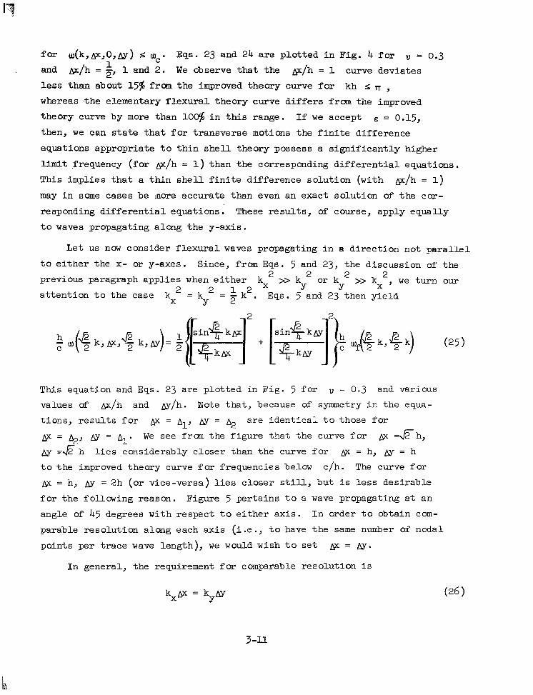
f o r w(k,fl,O,m) 5 wC. Eqs . 23 and 24 a r e p l o t t e d i n F i g . 4 f o r = 0.3 and m/h = z, 1 and 2. We observe that the f l /h = 1 curve deviates

less than about 15% from the imprm.ed theory curve for kh 5 , whereas - the elementary f lexural theory curve differs from the improved

theory curve by more than lo$ i n t h i s r a n g e . If we accept = 0.15, then, w e can state t h a t f o r t r a n s v e r s e motions t h e f i n i t e d i f f e r e n c e

equations appropriate t o t h i n s h e l l t h e o r y p o s s e s s a s ign i f i can t ly h ighe r

limit f requency ( fo r g /h = 1) than the corresponding different ia l equat ions

This impl ies tha t a t h in she l l f i n i t e d i f f e rence so lu t ion (w i th &/h = 1)

may i n some cases be more accurate than even an exact solution of the cor -

responding different ia l equat ions. These r e s u l t s , of course, apply equally

t o waves propagating along the y-axis.

1

Let us now cons ide r f l exura l waves propagating i n a d i r ec t ion no t pa ra l l e l

t o either the x- or y-axes. Since, from Eqs. 5 and 23, the discussion of the

previous paragraph applies when e i t h e r kx >> k or k >> kx , we tu rn our a t t e n t i o n t o t h e c a s e - k = $ k2. Eqs. 5 and 23 then y ie ld

2 2 Y Y

kx - Y

T h i s equation and Eqs. 23 a re p lo t t ed i n F ig . 5 f o r u = 0.3 and various

values of w/h and D/h . Note that, because of symmetry i n t h e equa-

t i o n s , r e s u l t s f o r p = @y = a r e i d e n t i c a l t o t h o s e f o r

p = 4, = A ~ . We see f rom the f igure that the curve for = a h ,

&r =& h l ies considerably c loser than the curve for ax = h, @y = h

t o t h e improved theory curve for f requencies below c/h. The curve for

& = h, = 2h (or v i c e - v e r s a ) l i e s c l o s e r s t i l l , but i s less des i rab le

for the fol lowing reason. Figure 5 p e r t a i n s t o a wave propagating a t a n

angle of 45 degrees wi th r e s p e c t t o e i t h e r a x i s . I n o r d e r t o o b t a i n com-

parable resolut ion a long each axis ( i .e . t o have the same number of nodal

points per t race wave length) , we would wish t o s e t g = &r. In general , the requirement for comparable reso lu t ion i s

k g = k & f X Y

3-11

Thus, if w e a n t i c i p a t e t h a t t h e s o l u t i o n t o a problem of i n t e r e s t w i l l be

cha rac t e r i zed by sho r t e r s t ruc tu ra l wave l e n g t h s i n one d i r e c t i o n t h a n i n

another, E q . 26 immediately yields the desired aspect ratio AX f o r

t h e f i n i t e d i f f e r e n c e mesh. To determine the mesh width magnitude , w e note

tha t the f in i te d i f fe rence f requency curves of Figures 4 and 5 cons t i tu te

a near ly optimum f i t below w = c/h t o t h e improved theory frequency

curve i f

Combining Eqs. 26 and 27, we f i n d t h a t , f o r a specif ied value of ky/kx,

the optimum mesh widths are given by

1/2 ,

optimum

Often it i s a l l b u t i m p o s s i b l e t o a n t i c i p a t e a va lue for

It i s then adv i sab le t o use a square mesh. In t h i s ca se , F igs . 4 and 5 suggest the use of the compromise mesh widths

= (F) 1 .2 (29 1 compromise c ompr omi se

Eqs. 28 and 29, in conjunct ion wi th F igs . 4 and 5 , y ie ld a limit frequency

for an optimum or compromise f i n i t e d i f f e r e n c e mesh of % M ws/2. However,

because the ra ther large negat ive curvature of the corresponding frequency

curves in t h i s r eg ion l eads t o undes i r ab le i naccurac i e s i n t he group ve loc i ty

c = dw/dk , we reduce the limit frequency t o g

3-12

This i s considerably above the limit frequency for continuum t h i n s h e l l

theory given by E q . 15, b u t i s s t i l l we l l below the improved theo ry l imi t

frequency given by Eq. 18.

Fina l ly , it i s i n t e r e s t i n g t o examine the reso lu t ion charac te r i s t ics

of f in i te d i f fe rence response computa t ions appropr ia te to the limit f r e -

quency of Eq. 30. If, f o r example, we s e t Aa/h = 1 and then take

A t = A t (see the f i r s t of Eqs . l J O ) f o r a one-dimensional t r a n s i e n t re-

sponse problem, we f i n d from Eqs .1.10, 17 and 30 t h a t &/Tm cS/6c 1/10,

where Tm = 2n/wm. Thus we have t e n computation points per period corres-

ponding to t he l imi t f r equency , which i s sa t i s f ac to ry . In con t r ac t , w e

f i n d from Fig . 4 t ha t t he limit wave number k (the value of k determined

by the Adh = 1 frequency curve f o r IJJ = wm) i s such that Aa/h 1/4, where Am = 2n/km. Thus w e have only four computation points per spatial

wave length corresponding t o t h e limit frequency. We conclude, therefore,

t ha t r e so lu t ion i s almost always be t t e r i n f i n i t e d i f f e rence r e sponse h i s -

tories than in the corresponding snapshots, a conclusion which i s supported

by numerous response computations in the p rev ious chapter . This f lexura l

resul t contrasts with the corresponding extensional resul t , which, because w(k) = ck f o r such motion, s ta tes that temporal resolut ion is i d e n t i c a l t o

spa t i a l r e so lu t ion .

c r

m

m

3.2.4 In t e rp re t a t ion . ~ ~~~ of Previous Numerical Results

Let us now make use of t he r e su l t s of t h i s s e c t i o n t o i n t e r p r e t some

of the numerical reslilts of Chapter 2 . We f i r s t c o n s i d e r Example 14 (Sub-

sect ions 2.2.4 and 2.4.2) , which involves the temporal smoothing of a uni-

form radial impulsive loading on a f r ee ly - suppor t ed cy l ind r i ca l she l l .

From Eq. 30, Eq. 17 and Table 2.2, we f ind t ha t t he limit frequency f o r

Aa/h = 1 computations i s

From Subsection 3.2.2, the excitation cutoff frequency for the

c t /a = 0.82 t r iangular pressure loading i s W

Thus, we are no t surpr i sed to see the margina l convergence behavior of the

acceleration computations of Fig. 2.39. The s a t i s f a c t o r y convergence

I

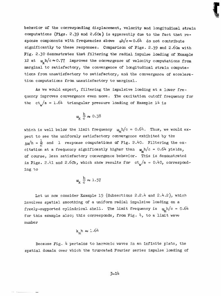
behavior of the corresponding displacement, velocity and longitudinal s t ra in

computations (Figs. 2.39 and 2.603) is apparent ly due t o t h e f a c t t h a t r e -

sponse components with f requencies abwe &/c= 0.64 do not contribute

s ign i f i can t ly t o t hese r e sponses . Comparison of Figs. 2.39 and 2 . 6 b with

F ig . 2 .30 demonst ra tes tha t f i l t e r ing the rad ia l impulse loading of Example

1 2 a t uxh/c =0.77 improves the convergence of velocity computations from

marginal t c sa t i s f ac to ry , t he convergence of l o n g i t u d i n a l s t r a i n computa-

t ions f rom unsa t i s fac tory to sa t i s fac tory , and the convergence of accelera-

tion computations from unsatisfactory t o marginal.

As we would expec t , f i l t e r ing the impulsive loading a t a lower f r e -

quency improves convergence even more. The exc i ta t ion cu tof f f requency for

t h e c t / a = 1.64 tr iangular pressure loading of Example 1 4 i s W

which i s well below the l i m i t frequency w h/c = 0.64. Thus, we would ex-

pec t t o s ee t he un i fo rmly s a t i s f ac to ry convergence exhibited by the

Aa/h = and 1 response computations of Fig . 2 .40 . F i l te r ing the ex-

c i t a t i o n a t a frequency significantly higher than %h/c = 0.64 y ie lds ,

of cour se , l e s s s a t i s f ac to ry convergence behavior. This i s demonstrated

in F igs . 2 .41 and 2.6m, which shaw re su l t s fo r e tw /" = 0.40, correspond-

i n g t o

m

1

L e t us now consider Example 1 5 (Subsections 2.2.4 and 2.4.2), which

involves spa t ia l smoothing of a uniform radial impulsive loaaing on a

f r ee ly - suppor t ed cy l ind r i ca l she l l . The limit frequency i s %h/c = 0.64

f o r t h i s example a l so ; t h i s corresponds, from Fig. 4, t o a limit wave

number

kmh M 1.64

Because F ig . 4 p e r t a i n s t o harmonic waves i n a n i n f i n i t e p l a t e , t h e

s p a t i a l domain over which the truncated Fourier series impulse loading of

Example 1 5 i s defined must be cons ide red i n f in i t e i n ex t en t . Hence w e take

the spa t ia l Four ie r t ransform of the loading t o f i n d a n e x c i t a t i o n c u t o f f

wave nuniber kx w (mmx + 2 ) n / ~ . For m = 5 max

kxh M 0.46

which i s much smaller than kih. Thus w e would expect t o see the uniformly

s a t i s f a c t o r y convergence exhibited i n F i g s . 2.43 and 2.61a. For m = 11 , max

kxh M 0.85

which i s approximate ly equal to the apparent l imi t wave number f o r Aa/h = 2

computations (Fig. 4 ) . We would the re fo re expec t t o s ee s a t i s f ac to ry con-

vergence behavior f o r a l l t h e A d h = 2 and Aa/h = 1 computations of

Figs. 2.44 and 2.61b. The f a c t t h a t t h i s i s not quite the case means t h a t

t he t rue l i m i t wave number f o r Aa/h = 2 computations i s somewhat less than

0.85. We do f ind uniformly satisfactory agreement between the Aa/h = 1

and Aa/h = - computations, huwever, which assures us t h a t s p a t i a l f i l t e r -

ing i s e f f ec t ive .

1 2

F or m max = 23 >

kxh M 1.64

which i s e q u a l t o t h e limit wave number above. We see, however, tha t agree-

ment between the Aa/h = 1 and &h = 2 computations of Figs . 2 .45 and

2 . 6 1 ~ i s not. uniformly sat isfactory. This mans that the t rue l imi t wave

nuniber i s somewhat l e s s t han 1.64 and suggests that Fig. 4 i s more r ead i ly

a p p l i e d t o t e m p o r a l f i l t e r i n g t h a n t o s p a t i a l f i l t e r i n g .

1

Fina l ly , i n view of Eqs. 28 (with k = 0), it i s not surpr i s ing tha t

t he Aa/h = 1 acceleration response curve of F ig . 2 .19 (as wel l as the iden-

t i ca l ve loc i ty response curve of Fig. 2 .26) i s the most physical ly meaning-

(see the discussion of Subsection 2.2.1). I n f a c t , t h e s e f i g u r e s imply

t h a t t h e Aar/h = 1 frequency curve l i es s u f f i c i e n t l y c l o s e t o t h e improved

theory curve over a s u f f i c i e n t l y wide kh-range t o p r e d i c t a c c u r a t e l y t h e

gross fea tures of the propagation of response discont inui t ies .

Y

3-15

..

3.2.5 Finite Difference Computational Procedure

Based on the results of t h i s and the previous chapter, it i s possible

t o c o n s t r u c t a recommended procedure for the appl icat ion of t h e ( t h i n s h e l l

t heo ry} f i n i t e d i f f e rence method i n s t u d i e s of t r ans i en t , l i nea r wave propa-

gation i n she l l s . Th i s p rocedure , spec ia l i zed t o t he d i sc re t i za t im method

used herein,

Step 1:

Step 2:

Step 3:

Step 4 :

S tep 5 :

Step 6:

Step 7:

i s as fol lows :

From Table 2.1, determine whether, fo r t he t ype of exc i t a t ion and the responses of i n t e r e s t , convergence can be expected t o be s a t i s f ac to ry . If no convergence problems are an t ic ipa ted , s k i p t o S t e p 5 ; i f convergence d i f f icu l t ies a re expec ted , p ro- ceed t o t h e n e x t s t e p .

From information pertaining t o the cha rac t e r i s t i c s of the ex- c i ta t ion (Sub-sect ion 3.2.2), determine an excitation cutoff frequency

Using E q s . 30 and 17, compute %. If wm > u) s k i p t o Step 5 ; i f u) i s appreciably smaller than wx, proceed to t he nex t svep . Temporally f i l t e r t h e e x c i t a t i o n a t w ; perhaps the best f i l t e r t o use i s t h e d i g i t a l f i l t e r o f % e f . 28, which completely suppresses exci ta t ion components with f requencies above the f i l ter cutoff f requency while introducing no amplitude or phase. d i s t o r t i o n i n t o t h e e x c i t a t i o n components w i th f r e - quencies below the f i l t e r cu to f f f r equency .

If the cha rac t e r i s t i c s t ruc tu ra l wave lengths along one ax i s a re expec ted to be shor te r t h a n those along the other axis, determine the mesh widths from Eqs . 28. I f there appears t o be no preferred direction, determine the mesh widths from Eq. 29.*

For temporal s tep-by-step integrat ion with an expl ic i t numer- i c a l scheme, s e l e c t t t ime s tep va lue s l igh t ly l ess than t h e c r i t i c a l time step given by the first of Eqs . 1.10. An implicit numerical scheme permits the use of a larger time s t e p . Check the accuracy of t he f i n i t e d i f f e rence so lu t ion e i the r through an error evaluation procedure incorporated into the numerical scheme or by means of add i t iona l runs with smaller mesh dimensions.

O"X * N

X'

Now the above recommended procedure i s based upon the short wave length

l imi ta t ions assoc ia ted wi th f lexura l she l l response . If the exc i t a t ion i s

* For very low frequency exci ta t ions, it i s poss ib l e t o u se mesh widths larger than those given by Eqs. 28 and 29. The number of nodal points per s t ruc- t u r a l wave length and/or the number of time points per temporal wave length (period) then becomes the dec id ing fac tor . (For frequency-wave number re- la t ionships , see Figs . 4 and 5 ).

3-16

pr imar i ly in -p lane , f lexura l e f fec ts p lay a small ro l e , and the f lexural

response l imi ta t ions no longer apply . In th i s case , Eq. 16 gives a limit

frequency of we w 2c/h , so t h a t mesh widths smaller than the shell thick-

ness may be prof i tably used. If the exc i t a t ion and responses of i n t e r e s t

are such that convergence diff icul t ies are ant ic ipated (see Table 2.1), it

i s advisable t o f i l t e r t h e e x c i t a t i o n a t we i n t h e manner of Step 4 i n

order not 'LO exceed the l imi t a t ions of t h i n s h e l l t h e o r y . Convergence of

the f ini te difference computat ions may then be expected f o r mesh widths

smaller than about 1 1 i o A e = i0(2'rc/we ) w h/3.

3.3 ADDITIONAL . ~~ CONSIDERATIONS REGARDING THIN SHELL AND IMPROVED THEORIES -~

This sec t ion br ie f ly d i scusses the so lu t ion of flexural response prob-

lems by the method of modal superposit ion and the method of c h a r a c t e r i s t i c s .

The resu l t s ind ica te tha t , whi le the modal convergence propert ies appropriate

t o improved theory a re genera l ly be t te r than those of elementary theory,

t h e a b i l i t y of improved theo ry t o t r ea t f l exu ra l r e sponse d i scon t inu i t i e s

may const i tute no real advantage.

3.3.1 Convergence ~~ Proper t ies of t he Method of Modal Superposit ion ~- "~-

The previous sections of t h i s chap te r have demonstrated t h a t t h e

major l imi t a t ion on the f lexural response computation capabili t ies of a

t h i n s h e l l f i n i t e d i f f e r e n c e code i s the r a the r l ong s t ruc tu ra l wave length

l imi t a t ion of t h i n s h e l l t h e o r y . Here we b r i e f l y examine t h e e f f e c t of

t h i s s t r u c t u r a l wave length l imi ta t ion on the method of modal superposi t ion.

We have observed i n Subsection 3.2.3 that limit frequency considera-

t ions for f in i te d i f fe rence computa t ions of shel l response reduce essent ia l ly

t o t h o s e f o r a simple beam. In addition, because convergence behavior i s a

s h o r t s t r u c t u r a l wave length phenomenon, boundary condi t ion detai ls are un-

important. Hence it i s s u f f i c i e n t t o f o c u s o m a t t en t ion on the t r ans i en t

response of a simply-supported beam.

Consider a simply-supported Bernoulli-Euler beam t h a t i s exci ted by

a unif o m impulsive load over a f i n i t e p a r t of i t s length. The pe r t inen t

kinetic energy, potential energy and v i r t u a l work expressions are (Fig. 6):

3-17 i

I '

where I i s t h e magnitude of the applied impulse. From the knmn

solut ion of the assoc ia ted f ree v ibra t ion problem, we write

m = l

Introducing Eq. 32 i n t o Eq. 31 and applying Lagrange's equation, we ob-

t a i n t h e m d a l equation of motion; solution of th i s equa t ion then leads

t o t h e s e r i e s s o l u t i o n f o r beam displacement

where the general ized mass Ma , natural f requency , and generalized

irnpul s e are given by I m

3-18

Because f l e x u r a l s t r e s s / s t r a i n i s p r o p o r t i o n a l t o a2w/a2 , we a r e

i n t e r e s t e d i n t h i s q u a n t i t y a s well as the k inemat ic quant i t ies d i sp lace-

m n t , ve loc i ty and acce lera t ion . Thus , s ince

m , m2 and m (Eq. 34), respect ively, i . e . , s ince Im N m and Mm N mo , we f i n d t h a t

I m J

0 -T and M vary as

2 -1 J s N m

w ~m -3 w ~m -. 1

We observe t h a t t h e series for displacement response converges quite

s a t i s f a c t o r i l y ; i n a d d i t i o n , it can be shown by a theorem of Dedekind

(Ref. 2 9 ) t h a t (for t > 0) the series far ve loc i ty and s t r e s s / s t r a i n con-

verge, although they do s o slowly. The series for acce le ra t ion response

c lear ly d iverges .

Let us nm cons ider a simply-supported Timoshenko beam under an

ident ica l loading . The per t inent k ine t ic energy and poten t ia l ex-

pressions for t h i s beam are (F ig . 6 )

R

T = $ $1 (i2 + (b2) dx

0

From t he known so lu t ion of the assoc ia ted f ree v ibra t ion problem, w e write

m = l W

m = l

(37 1

Introducing Eqs . 37 i n t o Eqs . 36 and t h e l a s t of Eqs . 31, and performing

the in tegra t ions , we obtain

m= 1

where i s g iven by the l as t of Eqs . 34. I m

Since there are now two modes for each value of m , f u r t h e r i n -

ves t iga t ion of the assoc ia ted f ree v ibra t ion problem i s required. Such

an invest igat ion (Ref . 2 7 ) yields as an accurate approximation for the

f i rs t mode

h2 2 where rm = -1 (7) . In t roduc ing t h i s i n to Eqs . 38 and applying

Lagrange's equation, we obtain the modal equation of motion whose solu-

t i o n i s

i n which I i s given by the las t of Eqs. 34 and m

3-20

where ($) i s given by E q . 39 and %2 i s given by the second of Eqs. 34. 1

The second mode, being orthogonal t o (z) , i s given by

1

In t roduc ing t h i s i n to Eqs . 38 and applying Lagrange's equation, w e obtain

the modal equation of motion whose so lu t ion i s

i n which I i s given by the las t of Eqs. 34 and m

, where (?) i s given by Eq. 42 and s2 i s given by the second of Eqs. 34.

2

The above resu l t s nm enable us t o wr i t e dawn our response solutions.

Since

w m ( t ) = w , W + w m2 ( t )

(45 1

we have, from Eqs . 37, 45, 40 and 43

3-21

Because f l e x u r a l s t r e s s / s t r a i n i s proport ional t o acp/& , we a re

in te res ted in th i s quant i ty , d i sp lacement , ve loc i ty and acce lera t ion .

Thus, s ince ( for l a rge m) I N m , ( ( P ~ / w ~ ) ~ r~ m -1 -1 0

m > % N m > Md N m J

and M cu m2 , we f i n d t h a t f o r l a r g e v a l u e s of m m2

w ~m -2 .. w r ~ m 0

Thus, not only i s the limit frequency higher for improved theory than for

elementary theory, but, from Eqs. 35 and 47, the modal convergence prop-

e r t i e s af the former a re genera l ly super ior to those of t h e l a t t e r .

3.3.2 Limitations of Improved Theory

She l l t heo r i e s i n gene ra l , and t h i n s h e l l t h e o r y and improved theory

in pa r t i cu la r , cons t i t u t e l ong wave length approximations t o e l a s t i c i t y

theory. Hence response solutions appropriate t o such theories can be

considered accurate only by appeal t o Saint-Venant ' s pr inc ip le , v iz . , t h a t t h e i n c l u s i o n of t h e e f f e c t s of neglected, self-equilibrating boundary

loads would l e a d t o s i g n i f i c a n t c o r r e c t i o n s i n t h e s t r e s s f i e l d o n l y i n

cer ta in h ighly loca l ized reg ions . Novozhilov and Slepian have demonstrated

in an excellent paper (Ref. 3 0 ) that , for suddenly appl ied loads, these

r eg ions a r e l oca t ed a t t he wave f r o n t s and a t t h e p o i n t s of load appl icat ion.

A s an example, cons ider the in f in i te p la te of Figure 7 t h a t i s ex-

cited uniformly along a s t r a igh t l i ne by a s tep shear load of t r i angu la r

prof i le th rough the p la te th ickness . Trea t ing th i s exc i ta t ion as the

superposit ion of a shear load which i s uniform through the thickness and

3-22

. . . . - .. ." . . . . . .. . .. _. .... .. . .. . . . .. , , . .... , .. , . .. . . . ... .

U a se l f - equ i l ib ra t ing shea r lcad that varies l inear ly th rough the th ickness ,

w e s e p a r a t e t h e t o t a l problem i n t o two component problems. The f i rs t has

been solved by Boley and Chao ( R e f . 18), who used improved p la te theory ;

t h e second has been solved by Novozhilov and Slepian, who used a p la te theory

one step "higher" than improved theory (Ref . 3 0 ) .

Boley and Chao present a snapshot of uniform shear stress only a t

t = 5 h / 2 a c = 1.45 h/c; the c losest comparable r e s u l t b y Novozhilov and

Slepian for l inear ly-varying shear stress is a t t = 3h/c = 1 .5 h/c.

Since the Novozhilov and Slepian results demonstrate only minor d ispers ion

over a time span of 0.05 h/c, t h e i r r e s u l t has been "moved back" and p lo t t ed

in F igu re 8a along with the Boley and Chao result. Because the magnitude

Of ne i ther sp ike a t the shear wave f ront decreases as t h e wave propa-

gates down the beam, this f igure demonstrates that the spikes which improved

shel l theory ignores can be comparable i n magnitude t o t h e s p i k e t h a t it

predic t s . We f ind, theref ore , that consis tent appl icat ion of a shell theory

t o t r a n s i e n t e l a s t i c wave propagation problems requires that one keep i n

mind the l imi t a t ions appropr i a t e t o Sa in t -Vernan t ' s p r inc ip l e a t bo th t he

points of load appl icat ion and a t t h e wave f ronts . This means t h a t compar-

isons between elementary and improved theory solutions can only be made

outs ide of these regions.

Unce r t a in t i e s a t t he wave f r o n t s may, i n f a c t , be only a minor problem,

i n view of F ig . 8b. This f igure shows the solut ion of Ref. 30 f o r t h e

moment response of a semi- inf in i te p la te t o a s tep moment applied uniformly

along i t s edge. We observe that the "further improved" theory demonstrates

a rapid "melting away" of t he ene rgy a t t he wave f r o n t which i s no t i n -

dicated by the improved theory. Thus, there i s a question whether, a t

reasonable distances from the region of load appl icat ion, short wave length

pulses predicted by improved (Timoshenko) s h e l l t h e o r y a r e a c t u a l l y p r e s e n t .

This i s i l l u s t r a t e d i n F i g . 9, which shows longi tudina l moment response

h/2

-h/2

f o r a semi- inf in i te cy l indr ica l she l l exc i ted by the impos i t ion of an

axisymmetric, radial, ramp-step velocity a t i t s end ( R e f . 16). The f i g u r e

3 -23

shows moment snapshots a t c t / a = 2 fo r va r ious ramp r i s e times. We ob-

serve tha t , even f o r a rise t ime as shor t as h/c , the ramp-step exci ta t ion

produces no response comparable t o t h e s p i k e c a u s e d b y t h e s t e p e x c i t a t i o n

( tr ise = 0 ) .

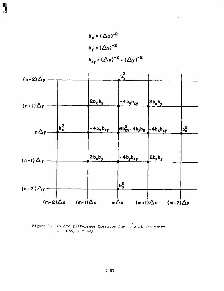
I

( n + 2 ) A y -

( n + l ) A y -

n A y -

4 x m,

3 -25

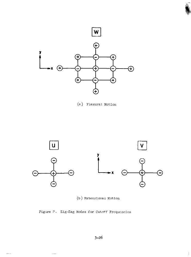
Y I

w

(a ) Flexura l Motion

Y

(b ) Extensional Motion

Figure 2 . Zig-Zag Modes f o r Cutoff Frequencies

3-26

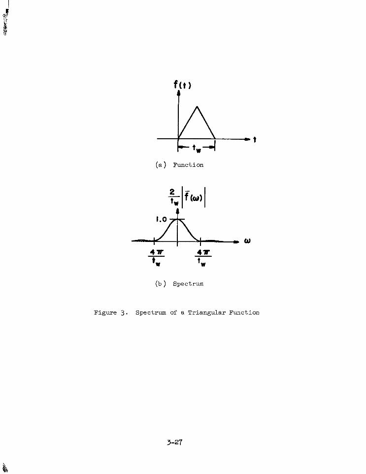
(a) Funct ion

(b ) Spectrum

Figure 3 . Spectrum of a Triangular Function

3-27

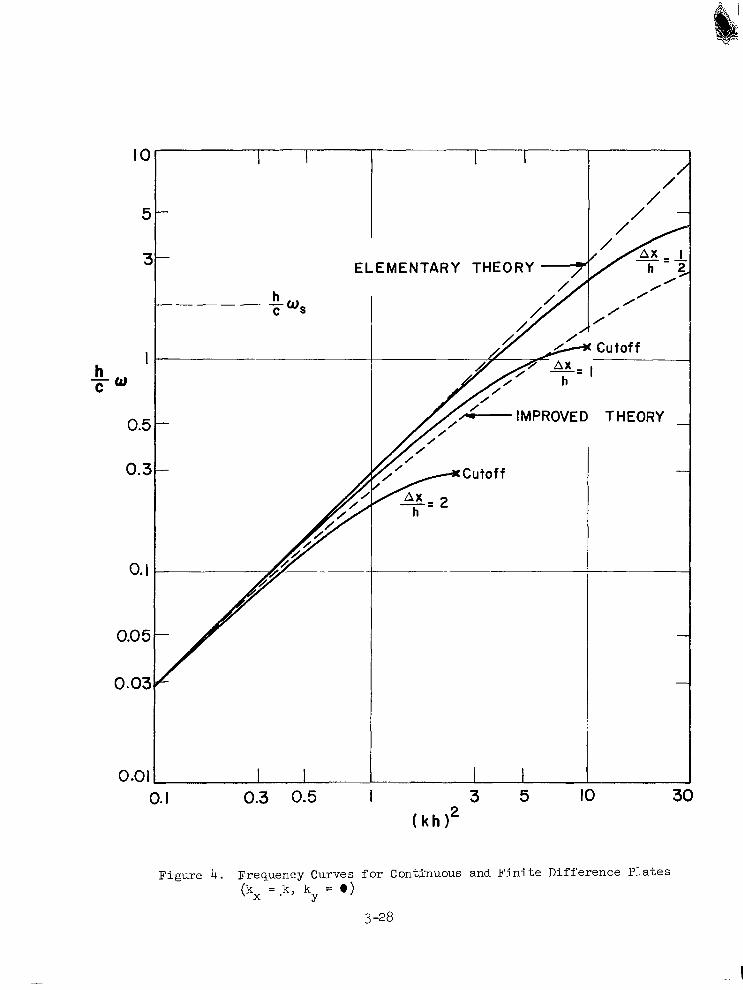
IO

5

z

I h cw

0.5

0.3

0. I

0.0 5

0.03

0.01

I I

h ””- 5 U S

I I 0. I 0.3 0.5 I 3 5 IO 30

( k h I 2

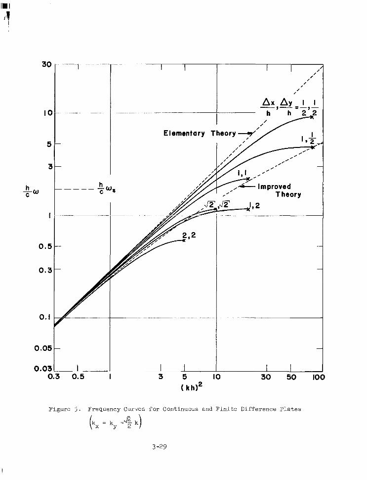
30

IO

5

3

h C "0

I

0 . 5

0.3

0. I

0.05

0.03

- "1"" "

h -"" C W S

0.3 0.5 I 3 5 IO 30 50 100

( kh I2

Figure 5 . Frequency Curves f o r Continuous and Fini te Difference Plates

3 -29

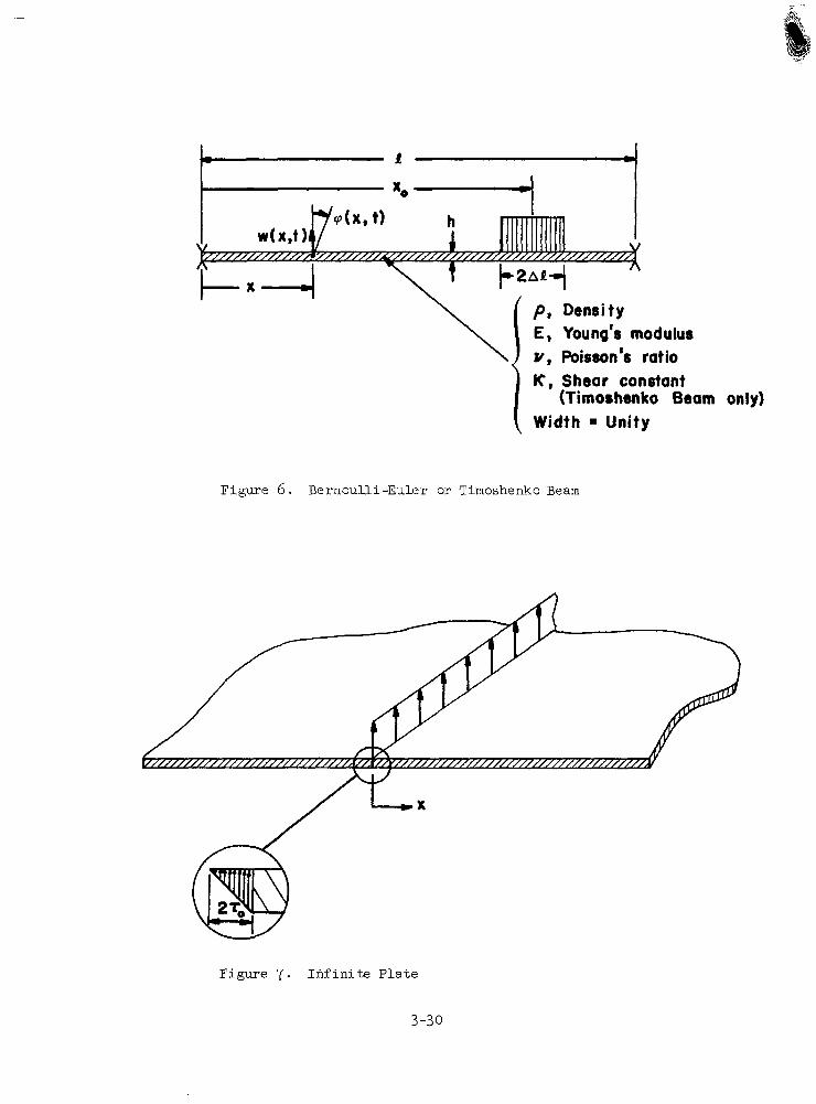
A

p, Density E, Young's modulus Y , Poisson's ratio IC, Shear constant

Width = Unity (Timoshenko Beam only)

Figure 6 . Bernoul l i -Euler or Timoshenko Beam

Figure 7. I n f i n i t e P l a t e

3-30

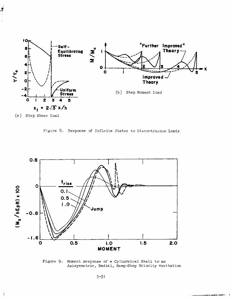
Theory

(b ) S t e p Moment Load

0 1 2 3 4 5

= 2m%/h (a ) Step Shear Load

F igure 8. Response of I n f i n i t e P l a t e s t o D i s c o n t i n u o u s Loads

0.8

0 0 e a Lrl a

\

s

I h

-0 .0 M

Y

-1.6 0.5 1.0 1.5 2.0

MOMENT

F i g u r e 9 . Moment Response of a C y l i n d r i c a l S h e l l t o a n Axisymmetric, Radial , Ramp-Step V e l o c i t y E x c i t a t i o n

3-31

Chapter 4

EXCITATION OF A SHELL WITH CUTOUTS

This chapter presents numerical resul ts for the response of a c i r c u l a r

c y l i n d r i c a l s h e l l w i t h f o u r i d e n t i c a l c u t o u t s t o unit impulse loads applied

a t one end. These loads, the f i r s t a longi tudinal load and the second a

rad ia l load , a re g iven by ( see F ig . A .2 for no ta t ion ) .

They have been chosen i r , order t o compare computed r e s u l t s f o r t h e r a d i a l

exci ta t ion with planned experimental resul ts (Ref . 31 ) .

A diagram of one-eighth of the she l l ' s sur face i s shown i n F i g . 1.

Included i n t h e f i g u r e i s information pertaining to the boundary con-

d i t ions se lec ted , , the po in ts a t which response his tor ies are computed,

and the QP and p- l i n e s f o r which response snapshots are obtained.

Although the mesh dimensions Ao/h = 1, aAp/h = rr/3 a r e n o t i n s t r i c t

accordance with E q s . 3 2 8 or 3.29, they constitute nearly optimum choices

t h a t c o n v e n i e n t l y f i t t h e s h e l l geometry. The t ime s tep, se lected in

accordance with Eqs. 1.10, i s cat/. = 0.04. The maximum computation time

corresponds t o the length of time requi-red f o r a d i s turbance t rave l l ing

a t t h e p l a t e v e l o c i t y t o t r a v e r s e a d i s tance equal to twice the l ength

of the she l l (c tmx/a = 4.8) .

Because the experiments of Ref. 31 r e l y c h i e f l y on the use of holog-

raphy t o measure shel l response, emphasis i s placed here on displacement

computat ions. Veloci ty , longi tudinal s t ra in and ef fec t ive s t ress responses

w i l l a l s o be considered, however. Axisymmetric results for the correspond-

ing v i rg in she l l wi th Aa/h = 1 and &h = demonstrate satisfactory

convergence for the responses to be discussed, except when indicated

otherwise.

I

4-1

4.1 LONGITUDINAL EXCITATION

Since the axisymmetric response of t h e v i r g i n s h e l l i s character ized

by (kca)2 M ( 2 ~ r / 0 . 8 ) ~ M 60, that response cons t i tu tes essent ia l ly non-

d ispers ive wave p ropaga t ion i n an i n f in i t e p l a t e (Appendix B ) . Hence w e

expect to observe the "s ta i rcase longi tudinal d isplacement his tor ies for

t h e v i r g i n s h e l l shown i n F i g . 2 . The corresponding results f o r t h e c u t

she l l a long t he l i ne p = 0 i n i t i a l l y d i s p l a y s i m p i e r e f l e c t i o n a t t h e l e f t

edge of the cu tou t fo r (Y = 0.4 and 0.6, as wel l a s s ign i f i can t sh i e ld ing

e f f e c t s for oy = 1.0 and 1.2. Well behind the wave f r o n t , however, the

e f f ec t s of the cu touts on she l l response a re no t very g rea t , except for a n

enhancement of r ad ia l r e sponse i n t he v i c in i ty of the cutouts . These effects

a r e even l e s s s i g n i f i c a n t a t p o i n t s a l o n g t h e l i n e $ = rr/12 , a s shown i n

F ig . 3 . Perhaps the c l ea re s t i nd ica t ion of t he sh i e ld ing e f f ec t s of the

cutouts i s given i n F i g . 4, which shows d i sp lacemen t h i s to r i e s a t po in t s

a long the l ine a/a = 1.2. While shielding effects are c lear ly discernable

in the f igure, they cannot be considered dramatic.

Longi tudina l s t ra in h i s tor ies , however, can exhibi t ra ther dramatic

e f f e c t s caused by the cutouts, as demonstrated in Figs. 5 and 6. Whereas

the s t ra in responses of the v i rg in she l l conta in negl ig ib le f lexura l con-

t r i b u t i o n s , s i g n i f i c a n t f l e x u r a l s t r a i n re.sponse does occur i n the cu t shel l

near the cu touts . Shie ld ing e f fec ts of the cutouts are shown i n F i g . 7, which presents s t ra in h i s tor ies a t po in ts a long the l ine a /a = 1 . 2 .

Although the cutouts have a subs t an t i a l e f f ec t on i n d i v i d u a l s t r a i n h i s t o r i e s ,

t h e i r impact on values of peak s t r a i n i s rather minor.

Figures 8-13 show displacement snapshots f o r the longi tudina l l ines

p = 0, n/12, and n/4 a t times ct/a = 0.8, 1.2, 2.0, 3.2, 4.0, and 4.4. These r e s u l t s seem t o add l i t t l e new information t o t h a t o b t a i n e d from

Figs. 2-4. They are included mainly for comparison wi th possible future

experimental results obtained by holographic techniques. They do i l l u s t r a t e ,

hcwever, that , a l though snapshats are very useful for the interpretat ion of

simple wave p ropaga t ion behav io r , t hey t end t o l o se t he i r e f f ec t iveness , a t

l e a s t f o r t h e purposes of these invest igat ions, as the behavior becomes

increasingly complicated. For complex response, then, response histories

seem t o emerge as the more e f f ec t ive i n t e rp re t ive t oo l .

Figures 14 and 15 are presented to ind ica te the degree of c i r c m -

ferentia1 non-axisymmetry produced near t he wave f ron t of t h e t r a n s i e n t

wave by the cu touts . From F ig . 14, w e observe that, a f t e r t h e wave f r o n t

has passed the cutouts, and e s p e c i a l l y a f t e r it has been reflected from

the boundary a t d a = 2.4 , longitudinal displacement response near the

wave f r o n t t e n d s t o become nuninally axisymmetric. Much of t h i s i s due t o

the steady growth of r t g i d body displacement. The tendency toward axisym-

metry, however, also charac te r izes the longi tudina l ve loc i ty and s t r a i n

responses near the wave f r o n t , e x c e p t i n t h e v i c i n i t y of the cutouts (Fig. 15 ). Radial displacement and velocity response tends t o become increasingly

p-dependent as time proceeds (Fig. 14).

A question that remains unanswered by the present computations i s

whether the presence of t he cu tou t s t ends t o f ac i l i t a t e t he l a rge - sca l e

t r a n s f e r of energy from extens iona l (pr imar i ly longi tudina l ) in to f lexura l

(pr imary rad ia l ) response . This , in fac t , seems t o be developing i n

Figs . 5a, 5b, 5c and 6b; on the other hand, it seems t o have been suppressed

i n F i g . 5d. A s a t i s f a c t o r y answer can only be provided by a long-time

solut ion, one t h a t i s not efficiently obtained by the present method. It

i s a problem of considerable interest , however, because such an energy

t ransfer can l ead to very l a rge rad ia l responses .

4 .2 RADIAL EXCITATION

A s implied ear l ier , the choice of the radial load used here was con-

s t ra ined by the charac te r i s t ics of an electromagnetic repell ing wire ex-

c i t a t i o n mechanism t o b e used i n planned experiments (Ref. 31). I n one

sense this i s unfortunate , s ince the resul t ing pulse load possess an ex-

c i ta t ion cu tof f f requency tha t i s about 2-1/2 'times the l i m i t frequency

given by Eq. 3.30. Hence, from Table 2.1, s t ress /s t ra in responses computed

with the present code a re inaccura te . This i s i l l u s t r a t e d i n F i g . 16, which shows l o n g i t u d i n a l s t r a i n h i s t o r i e s f o r t h e v i r g i n s h e l l computed

with Aa/h = 5 and 1. We observe that t h e peak responses computed with

Aa/h = 1 exceed the corresponding responses computed with Aa/h = p by

a s much a s 5 6 .

1 1

4-3

We a l so obse rve t ha t t he Aa/h = 1 responses of F ig . 16, espec ia l ly

f o r a/. = 0.4 and 1.0 , contain small ampl i tude o sc i l l a t ions a t t he mesh

cutoff frequency (Eq. 3.9) tha t a re no t p resent in the cor responding

Aa/h = $ responses. This i s due t c the f ac t t ha t t he exc i t a t ion cu to f f

frequency l i e s above the mesh cutoff f requency for Aa/h = 1 , bu t below

t h a t for a d h =

mesh does not.

a r e supe r io r t o

in Sec t ion 3 .2 .

In another

1 Hence the A@/h = 1 mesh "rings" while the Aa/h = 2 - 2 . This does not necessarily mean t h a t t h e Aa/h = $ responses

the Aol/h = 1 responses, however, for the reasons given

sense, the shortness of the pulse load i s only of minor

consequence, since we are mainly interested in displacement responses ,

which do exh ib i t s a t i s f ac to ry convergence behavior (Table 2 . 1 ) . Thus we

proceed t o F i g . 17, which shows displacement histories for the virgin

s h e l l ; we observe t h a t t h e f l e x u r a l wave f ron t t r ave l s a t abou t t he shea r

ve loc i ty c = [ F ( 1 - u ) ] ' l 2 c , while the longi tudinal wave f r o n t t r a v e l s

s l i g h t l y f a s t e r . Corresponding histories along the l ine $ = 0 on the

cu t she l l a r e shown i n F i g . 18. We immediately note the dramatic increase

in rad ia l d i sp lacement response a t the f ront edge of each cutout over the

corresponding response of the v i rg in she l l . The opposite occurs ( to a

lesser degree ) a t t h e back edge of each cutout. Only minor diff&rences

occur away from the cll touts.

1 S

Shie ld ing charac te r i s t ics of the cu touts a re ind ica ted in F ig . 19, which shows d isp lacement h i s tor ies a t po in ts a long the l ine a/a = 1.2.

The cutouts seem t o produce a moderate reduct ion in rad ia l d i sp lacement

response in the shadow regions behind them. Figures 20-23 show displace-

ment snapshots of both the virgin and cut shell displacement responses

a long the longi tudina l l ines $ = 0 , n/12 and n/4 a t t imes ct/a = 0.8, 1.2, 2.0 , 3.2, 4.0, and 4.4. Here too the response his tor ies seem t o be

less e f fec t ive as in te rpre t ive too ls than response snapshots for increas-

ing ly complex response. Figures 20-23 are included mainly for comparison

with experimental results obtained by holographic techniques.

Let us now examine the degree of non-axisymmetry in the displacement

response of a shel l . Figure 24 shows displacement snapshots along lines

of constant near and well behind the shear wave f r o n t . We see tha t ,

whi le the longi tudinal d isplacement response tends to be B-independent,

4-4

radial displacement response tends t o become increasingly fj-dependent.

This behavior i s the same a s t h a t observed i n F i g . 1 4 for the longi tudina l

exc i t a t ion .

We have he re t oo t he i n t e re s t ing ques t ion a s t o whether the presence

of the cutouts tends t o f a c i l i t a t e t h e l a r g e - s c a l e t r a n s f e r of energy

f rom ex tens iona l (pr imar i ly ax isymmetr ic rad ia l ) in to f lexura l (pr imar i ly

non-axisymmetric rad ia l ) response . Long-time solut ions are again required

t o answer th i s ques t ion .

4.3 SUMMARY

We have examined here the early-time response of a c y l i n d r i c a l s h e l l

w i t h c u t o u t s t o end pulse-loads whose spa t ia l wid th appropr ia te to p ropa-

g a t i o n a t t h e p l a t e v e l o c i t y i s only eight times the thickness of the

s h e l l . Computed resul ts indicate that the cutouts introduce no order-of-

magnit~~de changes in the response of t h e s h e l l . They do point t o moderate

s h i e l d i n g e f f e c t s i n shadow regions behind the cutouts, however. Further-

more, they suggest that the cutouts may f a c i l i t a t e t h e t r a n s f e r of load-

in jec ted ex tens iona l energy in to non-axisymmetric f lexural response, a

po ten t i a l ly dangerous s i tuat ion. Defini t ive conclusions about this phenom-

enon, however, await long-time solutions.

A broad pic ture of t he e f f ec t s of the cutouts on the response of the

s h e l l i s given i n F i g . 2 5 . For each po in t a t which a response history was

computed, two r a t i o s of peak response in the cu t she l l to the cor responding

peak response i n t h e v i r g i n s h e l l a r e shown. The responses chosen for

t h e s e r a t i o i n d i c a t o r s a r e , f o r t h e l o n g i t u d i n a l e x c i t a t i o n , l o n g i t u d i n a l

ve loc i ty and e f f e c t i v e s t r e s s and, fo r t he r ad ia l exc i t a t ion , r ad ia l ve loc i ty

and ef fec t ive s t ress . Veloc i ty response i s chosen because it i s often con-

s i d e r e d t o b e t h e most usefu l ind ica tor of damage po ten t i a l fo r a t t ached

s t r u c t u r a l systems (see, e.g., Ref. 3 2 ) . Effec t ive s t r e s s for the Mises

y i e ld su r f ace , i n t he form (Ref. 10)

4-5

i s chosen because it i s a use fu l measure of damage p o t e n t i a l for the s h e l l

i t s e l f . Even though the ve loc i ty and s t r a i n computations appropriate t o

the rad ia l loading a re no t en t i re ly sa t i s fac tor i ly convergent , they a re

considered adequate for the purposes of Fig. 25.

We observe i n F i g . 25 that the cutouts appear t o possess s ign i f icant ly

g rea t e r sh i e ld ing capab i l i t y fo r t he r ad ia l exc i t a t ion t han fo r t he l ong i -

t ud ina l exc i t a t ion . We a l s o observe that the related tendency toward

non-axisymmetry i s more p reva len t i n t he ca se of t h e r a d i a l e x c i t a t i o n .

The e f f e c t of reinforcement of the cutout on these r e su l t s would be of

considerable interest and a worthwhile subject of fu ture s tud ies .

4-6

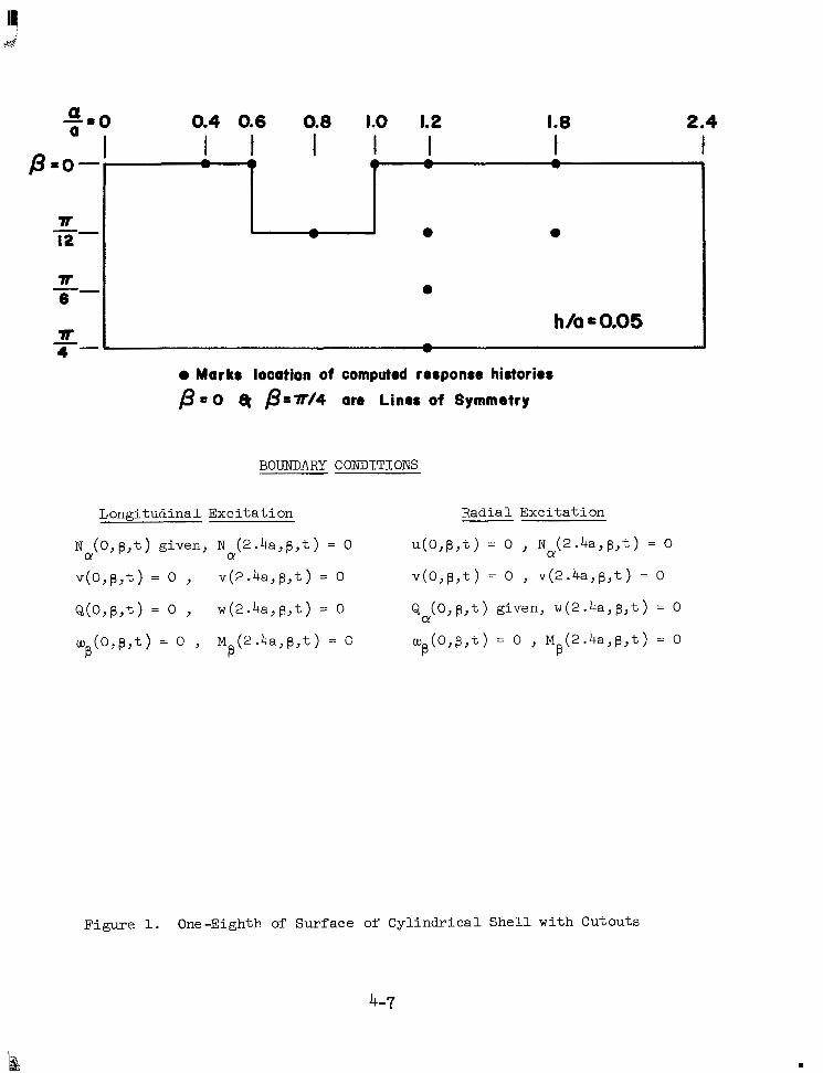
-80 0.4 0.6 0.8 1.0 1.2 a

a l I t I I I I I 1.8 2.4

J 0 Mark8 location of computed rerponre historims

p = o 4 P.7~4 are Liner of symmetry

BOUNDARY CONDITIONS

Longitudinal Exci ta t ion Radial Exci ta t ion

N ( O , p , t ) given, N ( 2 . 4 a , p J t ) = 0 u(O,p,t) = 0 , N ( 2 . 4 a J p , t ) = 0

v ( o , p , t ) = 0 , v ( 2 . 4 a J p , t ) = 0 v ( o , p , t ) = o , v ( 2 . 4 a J p , t ) = o

Q ( O , p , t ) = 0 , w(2 .4aJp , t ) = 0 Q ( O , B , t ) g iven, w(2.4aJpJt) = 0

w , ( O , p , t ) = 0 , M ( 2 . 4 a , p J t ) = 0

cy ty CY

CY

. p ( o J p J t ) = 0 J M ( 2 . 4 a , 9 p J t ) = ' 8 B

Figure 1. One-Eighth of Surface of Cyl indrical Shel l wi th Cutouts

4-7

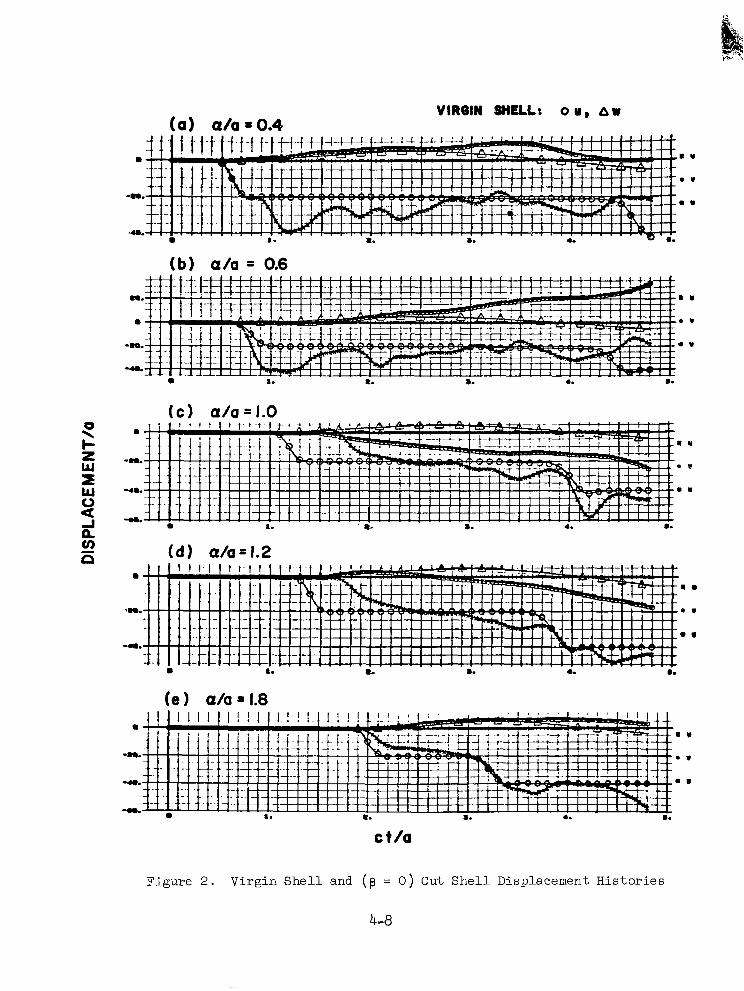
VIRBIN SHELLS o Y , CIw (a) o/a = 0.4

( c ) a / a = 1.0

a

-a.

a

-8m.

-4m.

( d ) a/a = 1.2

1. a. 4. D.

c t/a

Figure 2 . Virgin Shell and ( e = 0 ) Cut Shell Displacement Histories

4-8

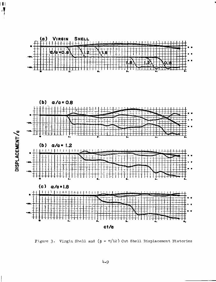
I I I

( a ) VIRGIN SHELL

-8e.

a

-am.

(b) a / a = 0.8

. . . . . . . . . . . . . . . . . . . . . . . . . . . 8. 4. .?

m m

* . ..

s m

* .

m .

c t/a

Figure 3. Vi rg in She l l and ( a = ll/12) Cut S h e l l Displacement Histories

4-9

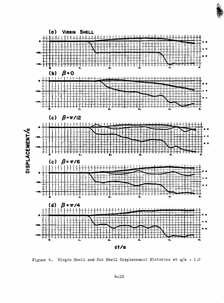
(a 1 VIRGIN SHELL a

-...

a

-00.

-.8.

a

-ma.

Figure 4. Virgin Shel l and Cut S h e l l Displacement Histories a t a/a = 1.2

4-10

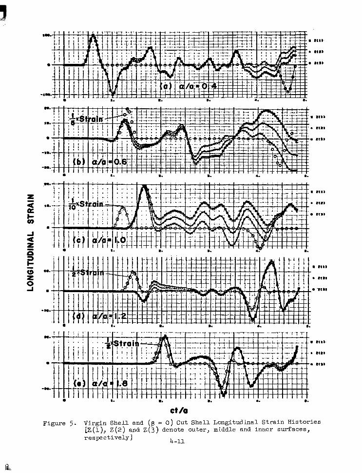
a 1. R. 8. S.

e 8t88

, m 8tDI

n.

8

10. . 0

-am.

-8..

S

e

8 t O

at88

If DD

ct /o Figure 5 . Virgin Shel l and ( p = 0) Cut Shel l Longi tudina l S t ra in His tor ies

[ Z ( l ) , Z(2 ) and Z ( 3 ) denote outer, middle and inner surfaces, respec t ive ly] 4 -11

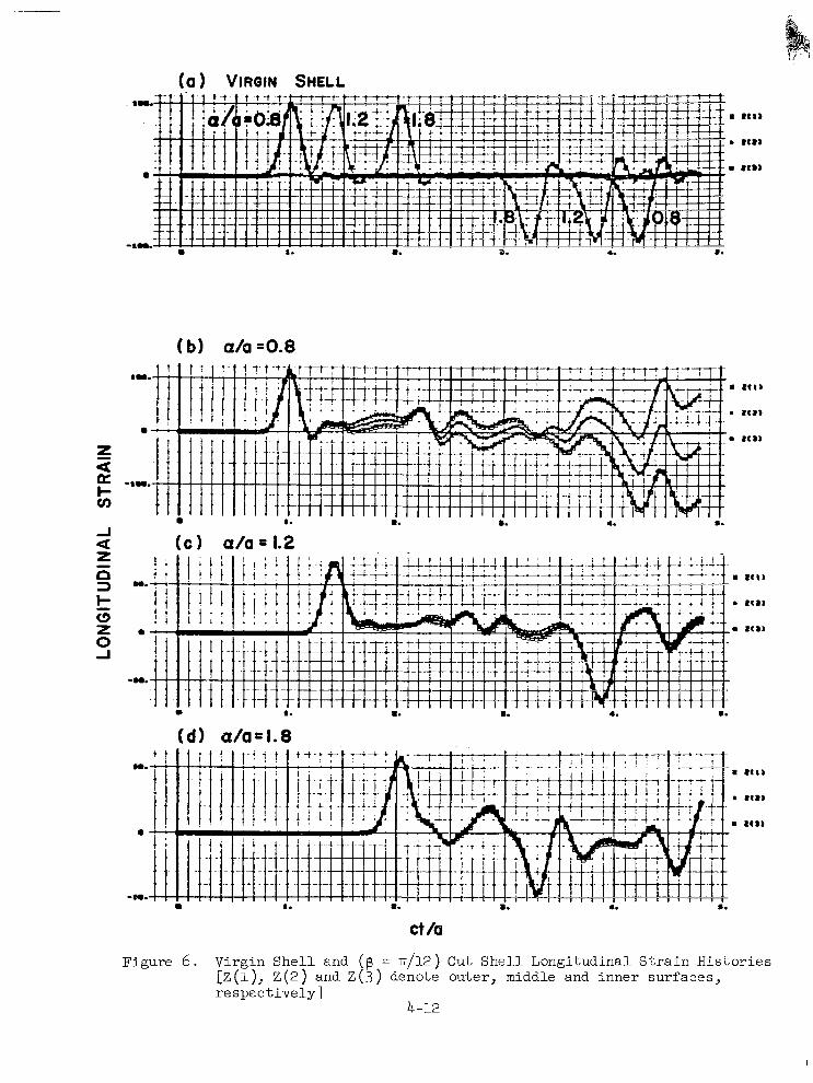
I...

-I...

( c ) a / a = 1.2

Figure 6 . Virgin Shell and ( p = ~r /12) Cut She l l Long i tud ina l S t r a in H i s to r i e s [Z(l), Z ( 2 ) and Z ( 3 ) denote outer, middle and inner surfaces , respec t ive ly]

4 -12

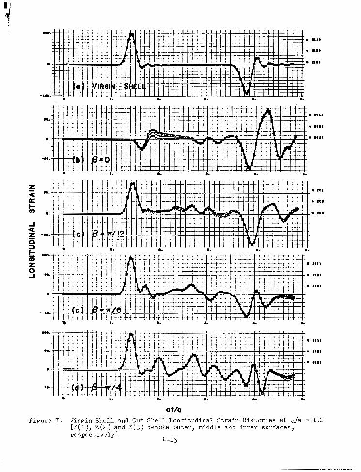
me.

e

-me.

sa.

H.

e -

'ii - m0"[

- L

I

I. R. a. 4. m.

1. R. . .

B.

1. R. a. 4.

Figure 7.

I

. e

I. R. a. 4. B.

c t/a Virgin Shel l and Cut She l l Long i tud ina l S t r a in H i s to r i e s a t a/a = 1.2 [ Z ( 1 ) , Z ( 2 ) and Z ( 3 ) denote outer, middle and inner surfaces, respec t ive ly]

4-13

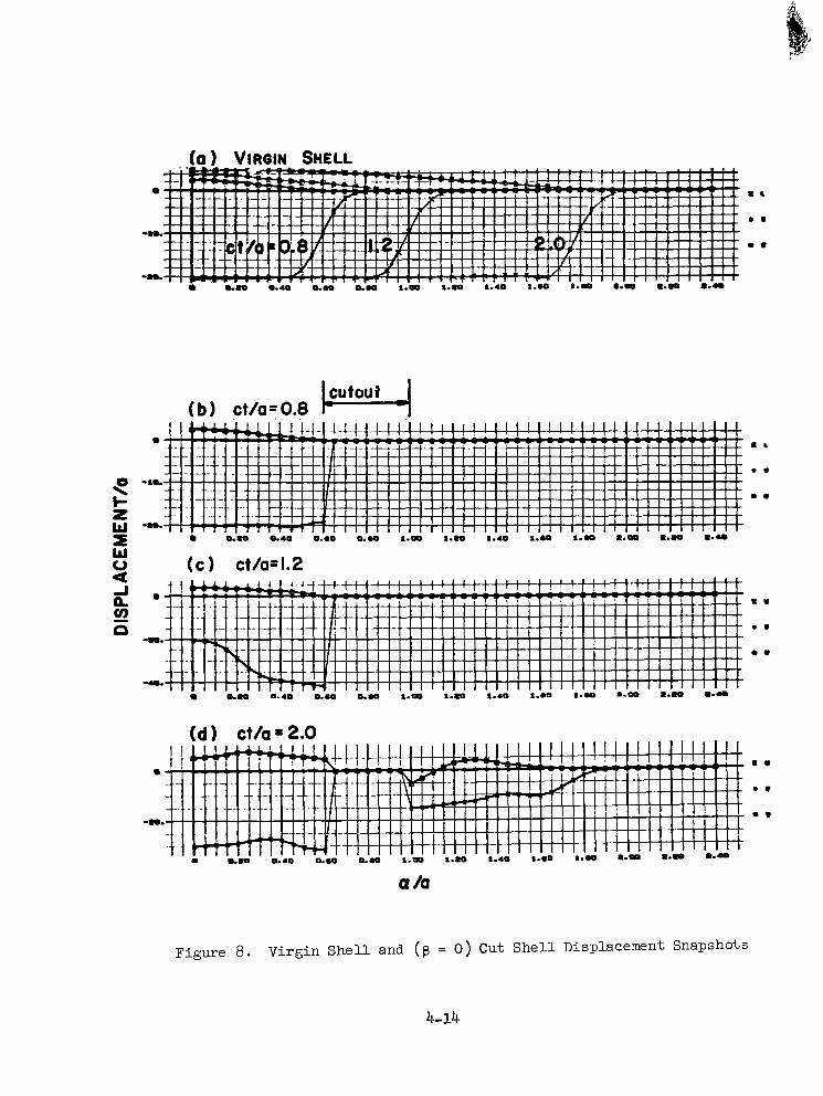
(a 1 VIRGIN SHELL

a

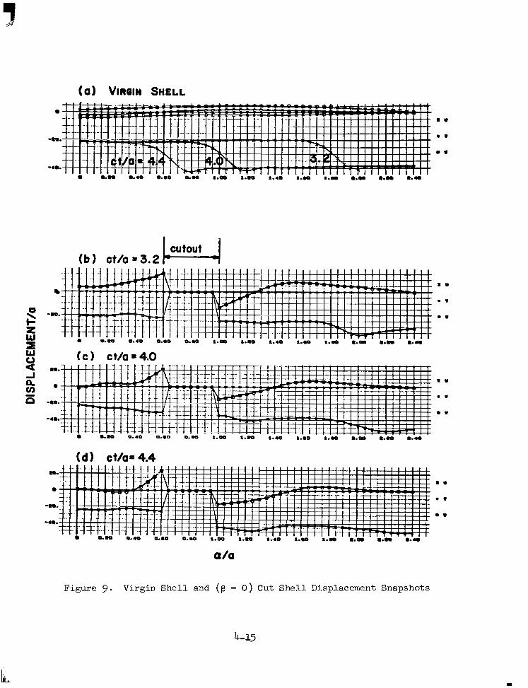
-sa.

cutout (b 1 ct/a = 3.2

o/a

I.

0 .

m .

Figure 9 . Virgin Shel l and ( p = 0 ) Cut S h e l l Displacement Snapshots

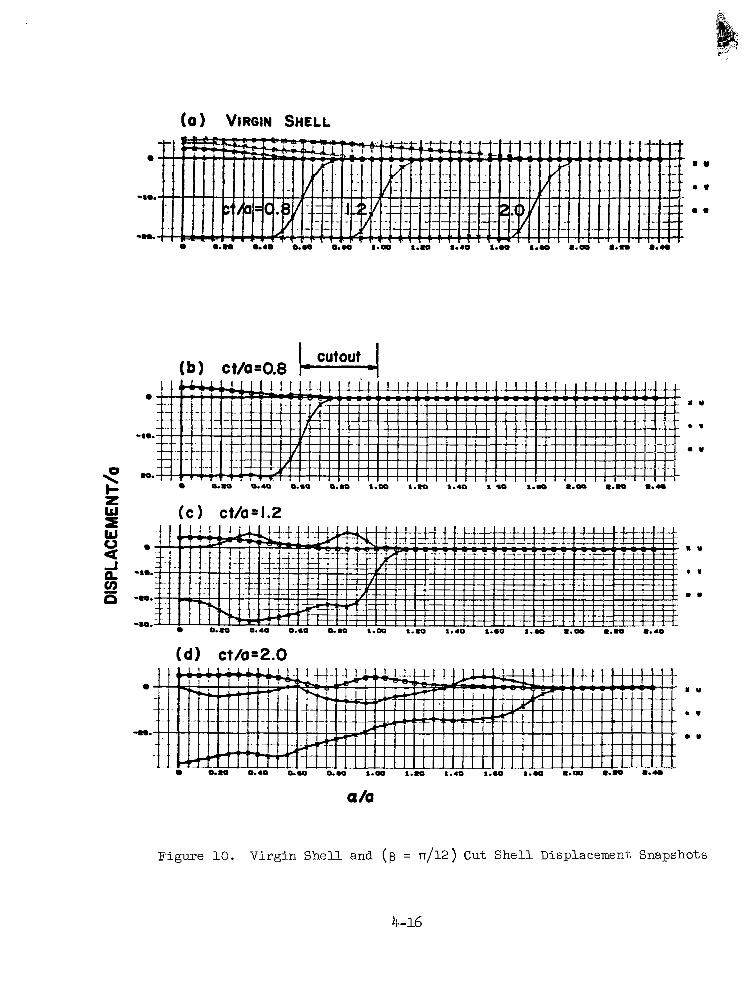
cutout 4 (b) ct/a=0.8

(c 1 ct/a=1.2

( d l cth.2.0

Figure 10. Virgin She

. Y

e 1

w m

a/a

11 and ( p = 17/12) Cut S h e l l Displacement Snapshots

4-16

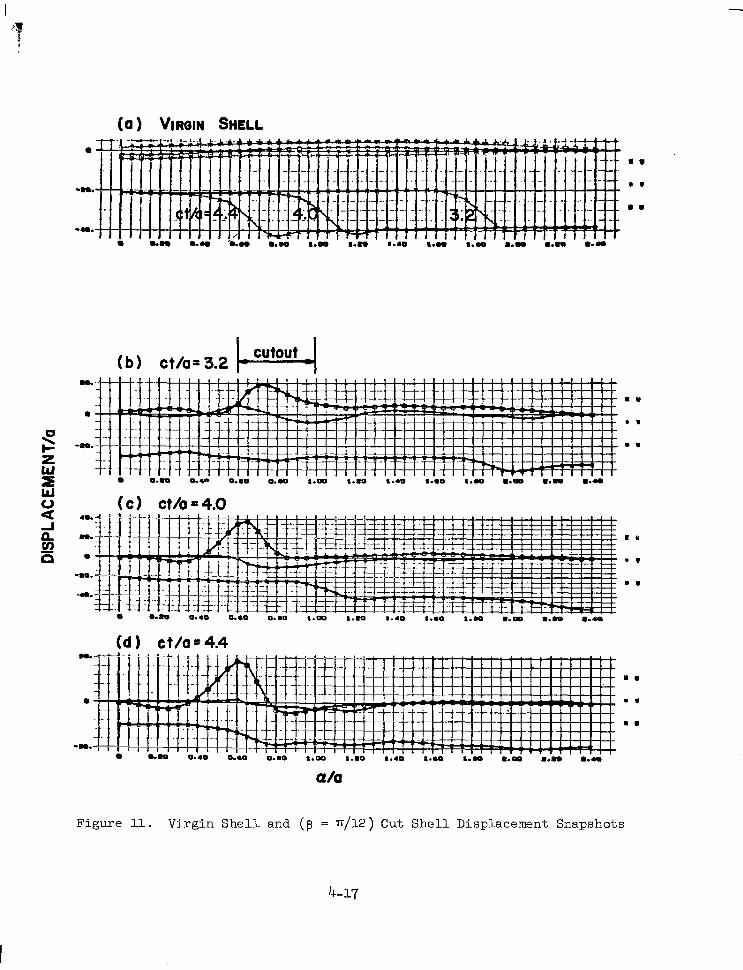
(a ) VIRQIN SHELL

-am

-...

(b) ct/a= 3.2

Figure 11. Virgin S h e l l and ( e = n/12) Cut Shell Displacement Snapshots

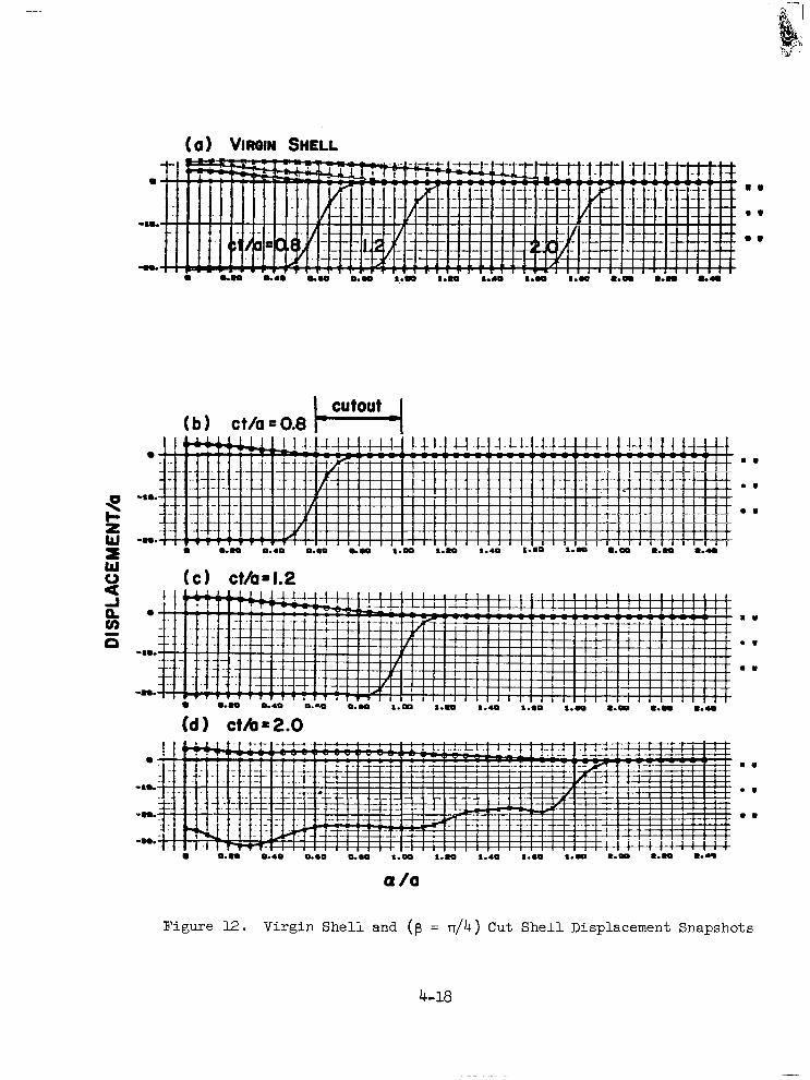
s 2 w L w

-le.

(b) c t h = 0.8 w

( c 1 ct/a= 1.2

e

-1..

-N.

(d 1 c t h = 2.0

I O .. m u

3 t s

4-18

.. ._ .......... ... , . .. . ... .. . . .. ...."...,... ,,. ..,..".._.,. ...

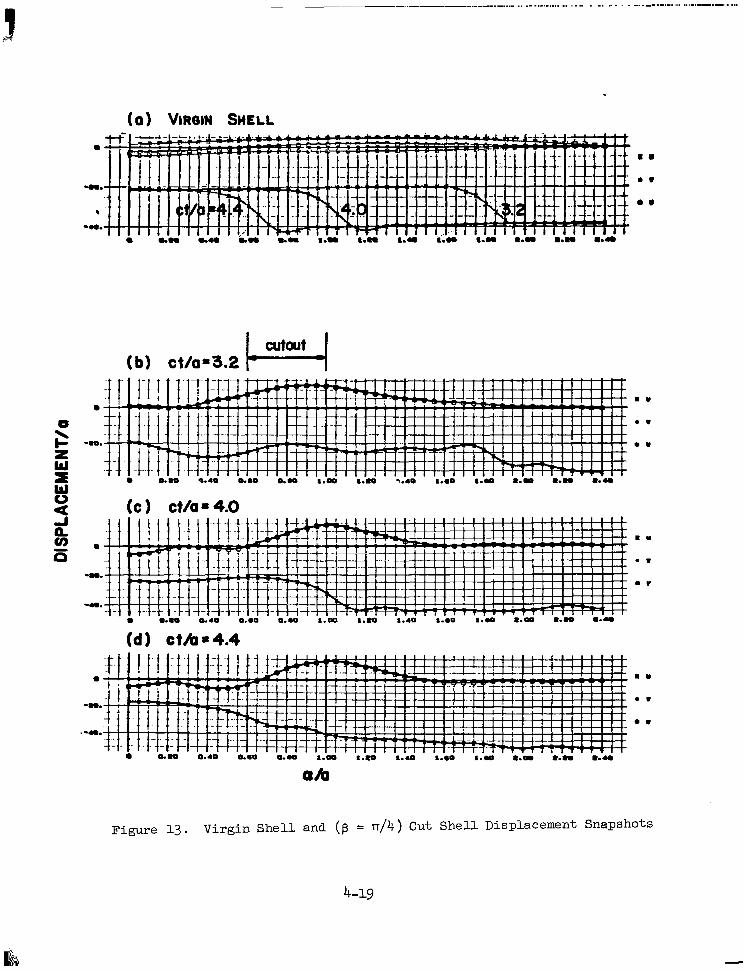
a

a

-a.

(a ) VIRGIN SHELL

(b) cVas3.2 H ..

(c ) ct/a = 4.0

a

-n.

-4..

(d ) ctrbr4.4

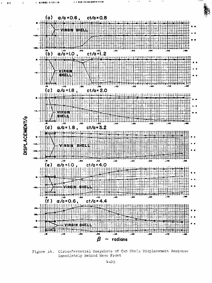
I IIII I

(a a h =0.6 , ct/a=0.8

-10.

-m. .a .LO -40 .SO ..O .m .a

. . " .

( b ) a?i=l.O , ct /a%2

-s. ml .LO .m ..o -40 .so .00 .m .a

"_

8 U

e .

m .

( c ) a h = 1.8 , ct/a= 2.0 ~~

.a .LO .to . ao . .O .m

( d l a h = 1.8, c t h n 3 . 2

Q

".

e a/a=I.O ct/a = 4.0

(f 1 a/a=0.6, ct /a=4 .4

- radians

8 U

0 .

m .

I U

0 .

m .

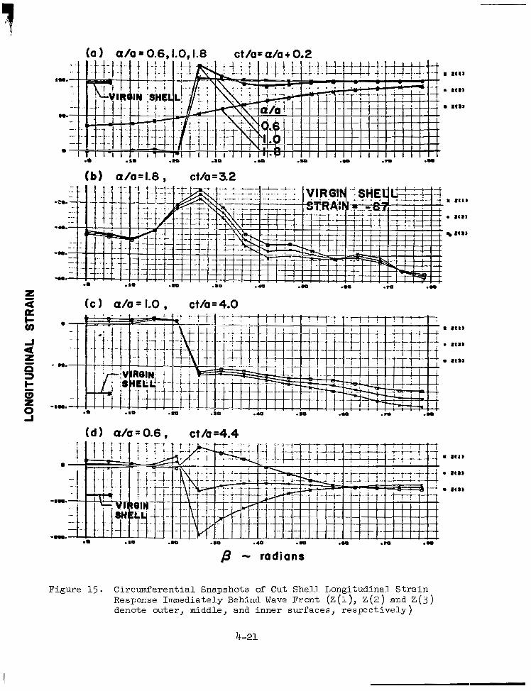
(a a/a = 0.6.1.0,1.8 ct/a= a/a + 0.2

(b) a/a=1.8, ct/a=32

I It18

0 It81

I t 8 8

.. .so .m . ao ..O .m .N

z (c 1 a l a = 1.0 . ct/a=4.0

.. .10 .m .m A

( d l a l a = 0.6 , ct/a=4.4

0

.. . so .m ..O .m .W .m .a

#3 - radians

Figure 15. Circumferential Snapshots of Cut Shel l Longi tudinal Strain Response Immediately Behind Wave Front (Z (1 ), Z ( 2 ) and Z ( 3 ) denote outer, middle, and inner surfaces, respectively)

4-21

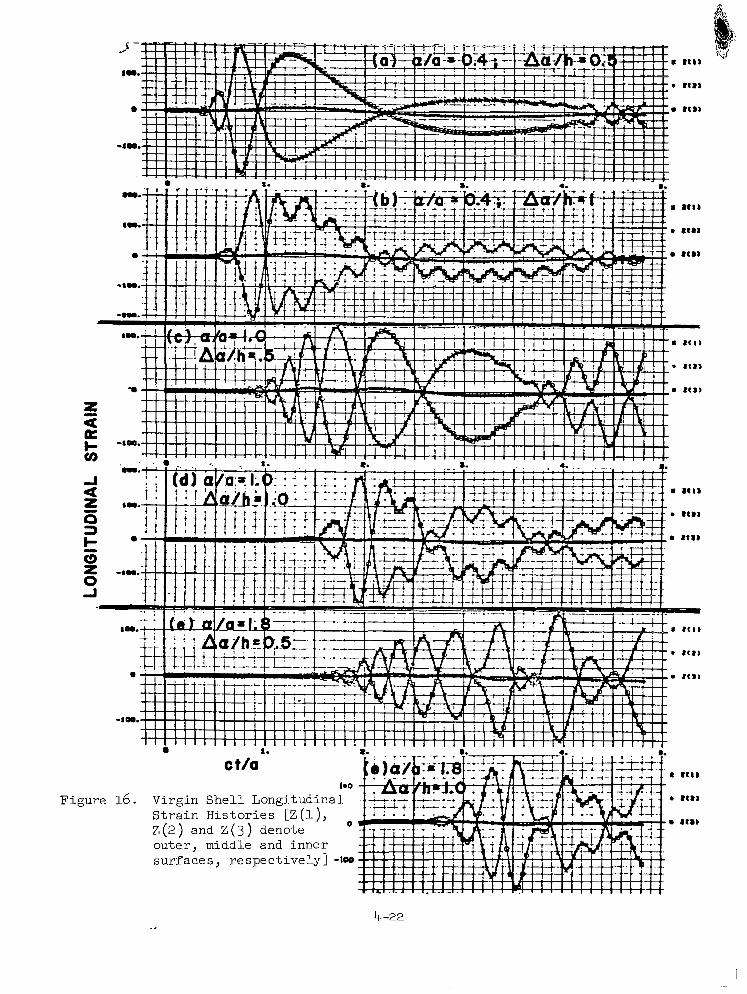
Fi

surfaces , respect ively] -1-

4 -22

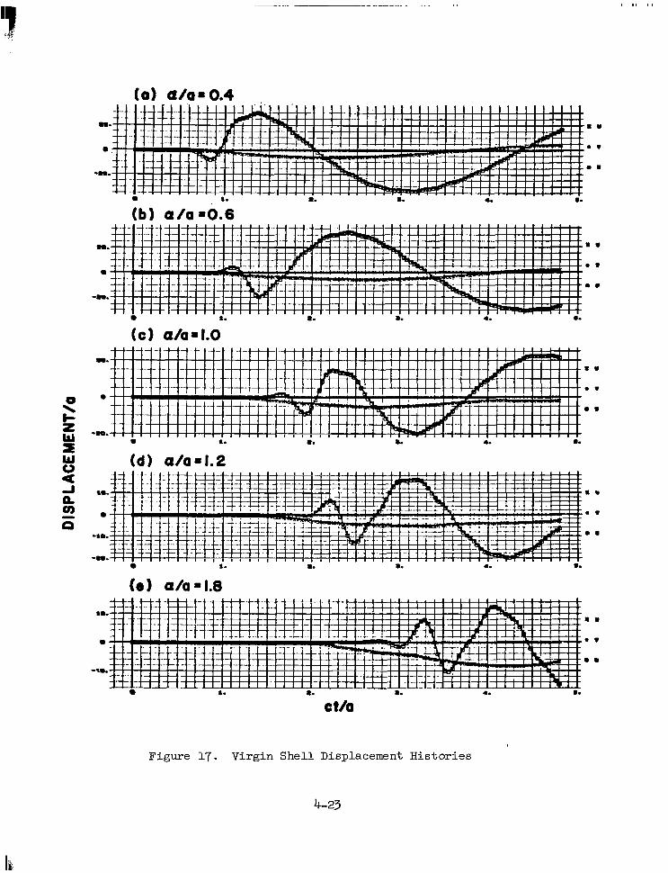
\ 0

t z w L

am. .(I .. -am. I.

(b) u / a =0.6

am. S O .. .. -am.

I.

8 .

I.

" 0 .

d u/o=1.2

1.. I.

8 .

-am- .. -am.

4. s.

Figure 17. Virgin She l l Displacement Histories

4-23

- -.

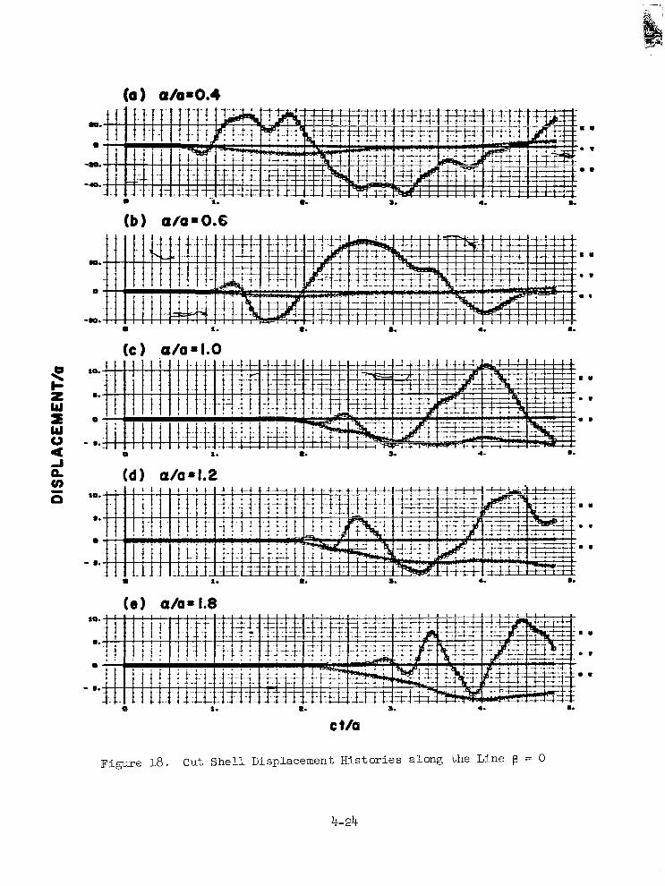
m.

0

I ,

~ . . I"-+ i ! ! ! !

1. R. .. 4. m.

(c 1 a/a = 1.0 . " . .

10. . _ ~

m.

0

- m. 0 1. R. a. 4- m.

10.

S.

- s. R. .. 4. m.

10.

0

- m.

0 1. R. 4.

c t/a

I.

0 . '. .

SI) .. 8 .

4- 24

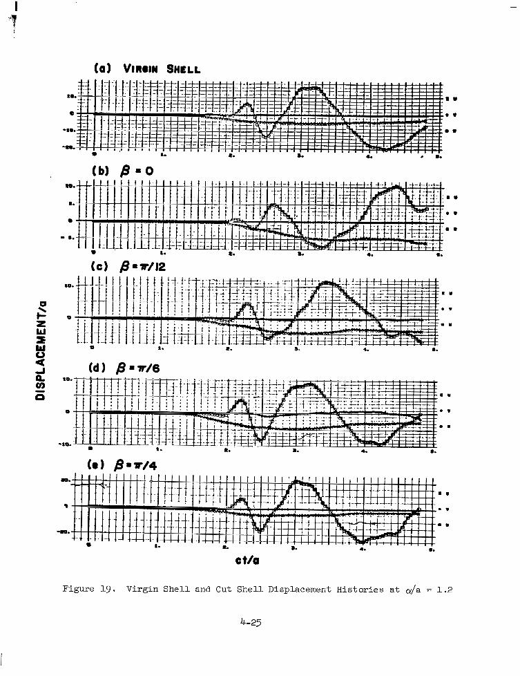
I

10.

0

-10.

0 1. m. 4. .. . Y

0 . ..

ao.

a

4. 0.

c t/o

Figure 19. Virgin She l l and Cut She l l Displacement Histories at cy/a = 1.2

4-25

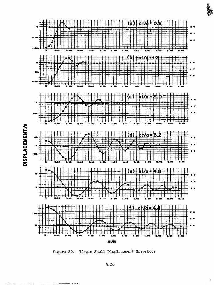
e m . n 0.- 0.00 aa 1.00 1.m 1.40 1.a 1.- ..a ..a 0.-

d o

I.

e .

m a

I Y

e .

m u

Figure 20. Virgin Shell Displacement Snapshots

4-26

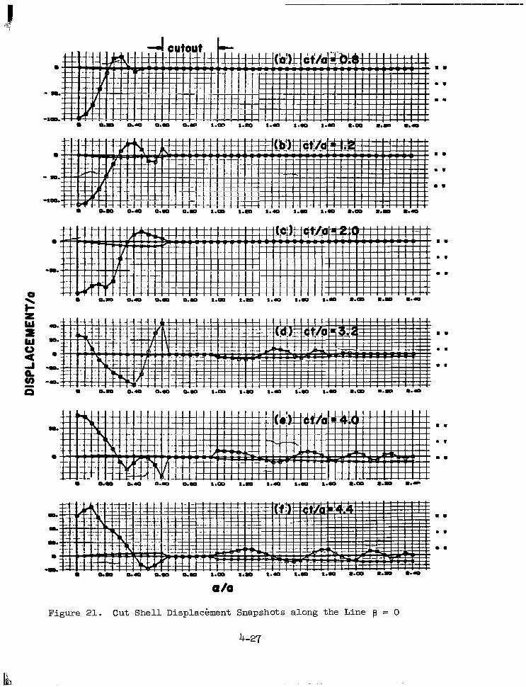
d -!

- m.

-1-

&a D.40 0.a 0 . 0 r.m 1.g 1.a 1.m s.m 8.m 8.m 8.a

. a

0 .

w m

a u

m w

w m

u/o

Figure 21. Cut S h e l l Displachment Snapshots along the Line p = 0

4-27

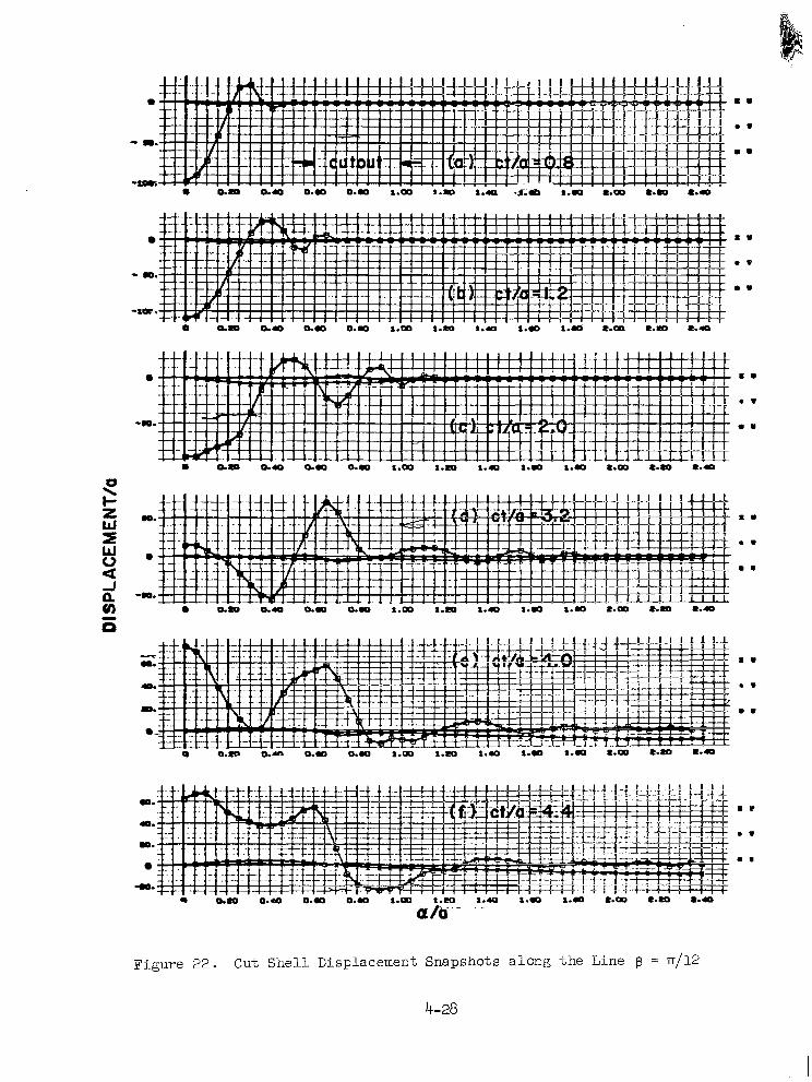
5 0

- a. -1w.

8

-a.

8 am aa aa 0.a r.m 1.m 1.10 1.a 1.a r.m r.m ).a

- a.

a.

m.

8

a.

a.

a.

4.

I.

0 .

m .

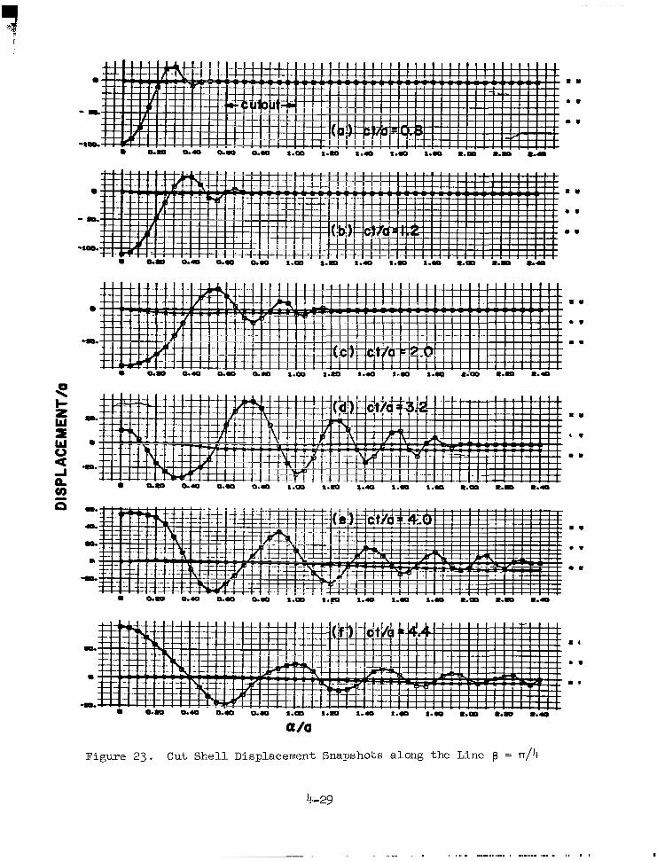
8

-.D.

-mm

-la

-a.

r L I I I - C J - I J u u ! ! ! ! ! ! ! ! ! I I ! ! ! ! ! ! ! ! ! ! ! ! ! ! ! ! ! ! ! ! ! ! ! ! ! L . .

8 W

r .

o w

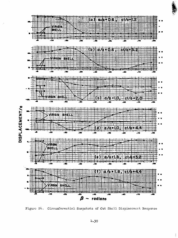
- 8.

-10.

.lo .b .R .a .m ...

m w

8 .

m m

m. m w

8 .

m w

m. .. m .

- radians

Figure 24. Circumferential Snapshots of Cut Shell Displacement Response

4-30

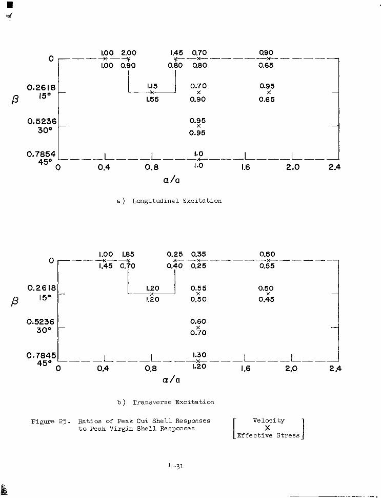
1.00 2.00 1.45 0.70 0.9 0

1.00 0.90 0.80 0.80 0.65

0.2618 1 l.k5 1 0.70 0.95 1.5 5 0.90 0.6 5

0 " "+6 tt-"----"-"

P 1 5 O

0.5 236 0.9 5 30° "" 0.95 X

4 5 O

X X

0.7854 L""I."" I. ""l""I" 0

0.4 0.8 I .o I .6 2.0 2.4 a /a

a ) Lalgi tudinal Exci ta t ion

1.00 1.85 0.25 0.35 0.5 0

1.45 0.70 0.40 0.25 0.55

0.26 I8 1 i.:O I 0.55 0.5 0

0.45

*-* M"-->t""" e""

P X

1.20 0.50 X

0.5236 0.60 0.70 30° X

0.7845 "_L""L"" 1.30 "" L""L"

0.4 0.8 1.20 I .6 2.0 2.4 a /a

b ) Transverse Excitation

Figure 2 5 . Ratios of Peak Cut S h e l l Respoilses Velocity t o Peak Virgin Shell Responses

Effec t ive S t ress

Chapter 5

CONCLUSION

This report contains: (1) a n a l y t i c a l and numerical s tudies per ta ining

t o t h e s o l u t i o n of t r ans i en t , l i nea r wave propagation problems i n t h i n s h e l l s

by the f in i te d i f fe rence method (Chapters 2 and 31, (2) a recommended com-

putat ional procedure for the use of the method (Chapter 3 ), and (3 ) a numer-

i c a l i n v e s t i g a t i o n of the response of a c y l i n d r i c a l s h e l l w i t h c u t o u t s t o

both longi tudinal and rad ia l t rans ien t exc i ta t ions (Chapter 4 ) . An out l ine

of major conclusions and recommendations for fu ture s tudy fo l lows:

5 . 1 MAJOR CONCLUSIONS

o The f i n i t e d i f f e r e n c e method accurately reproduces solutions of t he pa r t i a l d i f f e ren t i a l equa t ions of l i n e a r t h i n s h e l l t h e o r y i f t he mesh dimensions are appreciably smaller than the shortest s i g n i f i c a n t s t r u c t u r a l wave length characterizing the response of i n t e re s t . (Sec t ions 2 . 5 and 3 -1)

o The only inherent l imitat ion of t h e f i n i t e d i f f e r e n c e method i s i t s i n a b i l i t y t o reproduce accurately response discontinuities, a limi- t a t i o n t h a t a l s o a p p l i e s t o t h e method of modal superposit ion but does not apply t o t h e method of charac te r i s t ics . (Sec t ions 2 .5 and 3.1)

o The shor t wave length l imi ta t ions of th in she l l (Bernoul l i -Euler ) theory create s ignif icant convergence diff icul t ies in computed responses t o c e r t a i n t y p e s of t ransverse exci ta t ions. (Sect ions 2 . 5 and 3 . 2 )

o Proper selection of f i n i t e d i f f e r e n c e mesh dimensions, combined,in some cases, with temporal smoothing of the exc i ta t ion , increases the frequency range of th in she l l (Bernoul l i -Euler ) theory by a f a c t o r of th ree for t ransverse exc i ta t ions . (Sec t ion 3 .2)

o Convergence d i f f i c u l t i e s i n t h e c a s e of t ransverse exc i ta t ions may be mater ia l ly a l leviated through the use of improved (Timoshenko) theo ry ; t he ab i l i t y of improved theo ry t o t r ea t f l exu ra l r e sponse d i scon t inu i t i e s , however, may const i tute no real advantage. (Sections 3.2 and 3.3)

o Cutouts i n a c y l i n d r i c a l s h e l l e x c i t e d a t one end by axisymmetric longi tudina l and radial pulse-loads produce moderate changes i n shel l response during ear ly and intermediate t imes; the cutouts may, however, fac i l i t a te the undes i rab le l a te - t ime t ransfer of load-in jected extensional energy into non-axisyxnetr ic f lexural response (Section 4.3)

5-1

5.2 RECOMMENDATIONS FOR l?UTURE STUDY

o The s tudies of Chapter 2 should be extended t o inc lude exc i ta t ions t h a t a r e s p a t i a l l y narrow in t he c i r cumfe ren t i a l dimension; numeri- c a l s t u d i e s a r e r e q u i r e d .

o The computational procedure recommended in Sec t ion 3.2, e spec ia l ly tha t a spec t which dea l s w i th t empora l f i l t e r ing of the exc i ta t ion , should be thoroughly tested; numerical studies are required.

o The advantages and disadvantages associated with the use of improved theory as opposed t o t h e use of t h in she l l t heo ry shou ld be de f in i t e ly es tab l i shed; bo th ana ly t ica l and numerical s tudies are required.

o The shor t wave length l imi ta t ions of improved theory should be determined with the techniques of Ref. 30; ana ly t i ca l s tud ie s a r e required.

o The degree t o which cutouts may f a c i l i t a t e t h e l a t e - t i m e t r a n s f e r of load-injected extensional energy into non-axisymmetric f lexural response should be determined; solution by the method of modal superposi t ion i s sugges ted for th i s t ask .

o The e f f e c t s of re inforced cu touts , s t ruc tura l ( r ing and longi tudina l ) s t i f f e n e r s , and attached mechanical systems on the propagation of t r a n s i e n t waves in shel ls should be investigated; numerical studies a re requi red .

o The e f f e c t s of geometric and material nonlinearit ies on the genera- t i o n and propagation of t r ans i en t waves in shells should be examined; numerical s tudies are required.

o A comprehensive study that compares f in i t e d i f f e rence , f i n i t e e l emen t , modal superposit ion and c h a r a c t e r i s t i c s methods for the so lu t ion of problems involv ing t rans ien t l inear wave propagat ion in shel ls should be performed.

5-2

Appendix A

THE STAR CODE

The f i n i t e d i f f e r e n c e computer program. STAR (Shel l Transient Asymmetric

Response) i s capable of computing the two-dimensional, finite-amplitude

response of ine las t ic she l l s wi th unre inforced cu touts to mechanica l and

thermal t ransient loads. The code i s based on t h e g e n e r a l t h i n s h e l l

equations of Ref. 6 and on cons t i tu t ive equat ions for a temperature-

dependent, work-hardening material. A de ta i led descr ip t ion of the code

i s given in Ref. 10; this appendix merely defines pertinent notation and

describes improvements made i n t h e code a s p a r t of the present s tudy.

A . 1 GEOMETRIC NOTATION

The middle surface of t h e s h e l l i s shown i n F i g . 1. The l i n e s of

pr incipal curvature , CY = constant and $ = constant , are selected as the

coordinates of the middle surface of t h e s h e l l . The coord ina te i n t he

d i rec t ion of the inward normal t o t h e middle surface i s denoted by z .

We see that the coordinates are such that ( a , $, z ) form a right-handed

system. The element of a rc l ength ds on the middle surface i s given by

where A ( a, p ) and B( a, p ) are the Lame ' parameters for the middle

surface of the undeformed she l l . F igure 1 a l s o shows the p r inc ipa l

r a d i i of curvature r the displacement components u, v, w , and

the ro t a t ion components . The components (u, u) ), ( v, we) ' and w a re t aken pos i t i ve i n t he d i r ec t ion of increasing cy, and z , respec t ive ly .

a, r p ' wcy, w$ CY

If (Y denotes e i ther the a rc l ength measured along the generator from

the apex of a c i r c u l a r cone or t he end of a c i rcu lar cy l inder , and i f $ i s

the angular coord ina te in the c i rcumferent ia l d i rec t ion , then the Lame' par-

ameters and rad i i 6f curvature f o r these sur faces a re es follows :

A - l

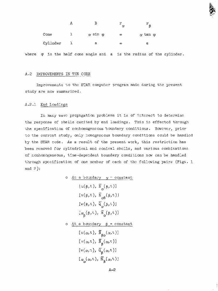
A B r CY

r B

Cone 1 (Y s i n cp m CY t a n cp

Cylinder 1 a CD a

where cp i s the half cone angle and a i s the rad ius of the cy l inder .

A .2 IMPROVEMENTS I N THE CODE

Improvements t o t h e STAR computer program made during the present

s tudy are now summarized.

A.2.1 End Loadings

I n many wave propagation problems it i s of i n t e r e s t t o determine

the response of she l l s exc i ted by end loadings. This i s effected through

the spec i f ica t ion of nonhomogeneous boundary condi t ions. However, p r io r

to the cur ren t s tudy , on ly homogeneous boundary conditions could be handled

by the STAR code. A s a r e s u l t of the present work, t h i s r e s t r i c t i o n has

been removed f o r c y l i n d r i c a l and con ica l she l l s , and various combinations

of nonhomogeneous, time-dependent boundary conditions now can be handled

through specif icat ion of one member of each of the fo l lawing pa i r s (F igs . 1

and 2 ) :

o A t a boundary p = constant ~-

A-2

A . 2 . 2 One-Dimensional Problems

The STAR code, which was o r ig ina l ly developed

response of she l l s , can, of course , a l so accommodate

f o r t h e asymmetric

one -dimensional

problems, such as axisymmetric shells under axisymmetric loads or rings

s u b j e c t e d t o asymmetric loads. However, p r i o r t o t h e c u r r e n t s t u d y ,

spec ia l l og ic had not been provided for such problems. Thus, t o d e f i n e

the f i n i t e d i f f e rence expres s ions fo r spa t i a l de r iva t ives i n t he gene ra l

equations, it was necessary t o s p e c i f y a minimum of f ive nodal po in ts a long

each of the g r i d l i n e s i n t h e a and $ d i rec t ions . For one-dimensional

problems (such as many of the problems considered i n Cnapter 2) , th is pro-

cedure i s obviously qui te ineff ic ient and hence, fox- reasons of economy of

computer run time, the code was modified t o t r e a t one-dimensional problems

more e f f i c i e n t l y . A s a r e s u l t of the mcdification, only one s e t of g r id

l ines (rather than two) needs t o be specified; th is l e a d s t o a reduction

of run time by a f a c t o r of approximately f ive.

A.2.3 Kore Accurate Computation of Velocity ~

To descr ibe the expl ic i t numerical technique employed i n t h e com-

putat ion Of the ve loc i ty components a t e a c h mesh point , it i s s u f f i c i e n t

to cons ider the normal component, ; ( t) , which had been previously corn-

puted from

where ( * ) denotes d i f fe ren t ia t ion wi th respec t to t ime t , and A t i s

the t ime step. Equation 2 can be derived either from a Taylor series

representat ion of G ( t ) , with re ten t ion of only linear terms, or from a

forward f in i te d i f fe rence approximat ion for v(t-At). The t runca t ion

e r r o r < ( t ) as computed from Eq. 2 i s O ( A t ) 2 . * A t runca t ion e r ro r of

order ( A t ) 3 i s achieved if the ve loc i ty i s instead computed from

st o( A t ) 2 denotes a term with an error of order ( A t ) '

A-3

, _. ... . .

This expression may be der ived from the cen t r a l d i f f e rence r ep resen ta t ion

W(t-At/2) - 1 [ G ( t ) - G ( t - A t ) ] A t

and the approximation

The l a s t t e r m i n Eq. 3 i s computed from the equation of motion in t he

normal d i rec t ion , namely,

Y ( t ) = F Z ( t ) - C Z G ( t ) ( 6

where Cz i s a viscous damping coe f f i c i en t and F i s a known funct ion

of the displacement and the loads. The introduct ion of E q . 6 i n t o E q . 3 yields the fol lowing O ( expl ic i t express ion f o r t he ve loc i ty t ha t

i s cur ren t ly employed i n t h e STAR code:

Z

A-4

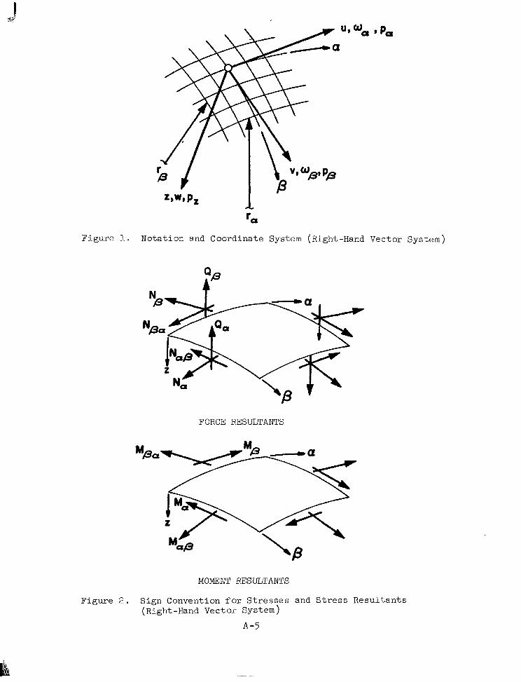
re Figure 1. Notation and Coordinate System (Right-Hand Vector System)

FORCE RESULTANTS

MOMZNT RESULTANTS

Figure 2 . Sign Convention f o r S t resses and St ress Resul tan ts (Right -Hand Vector System)

A -5

" .

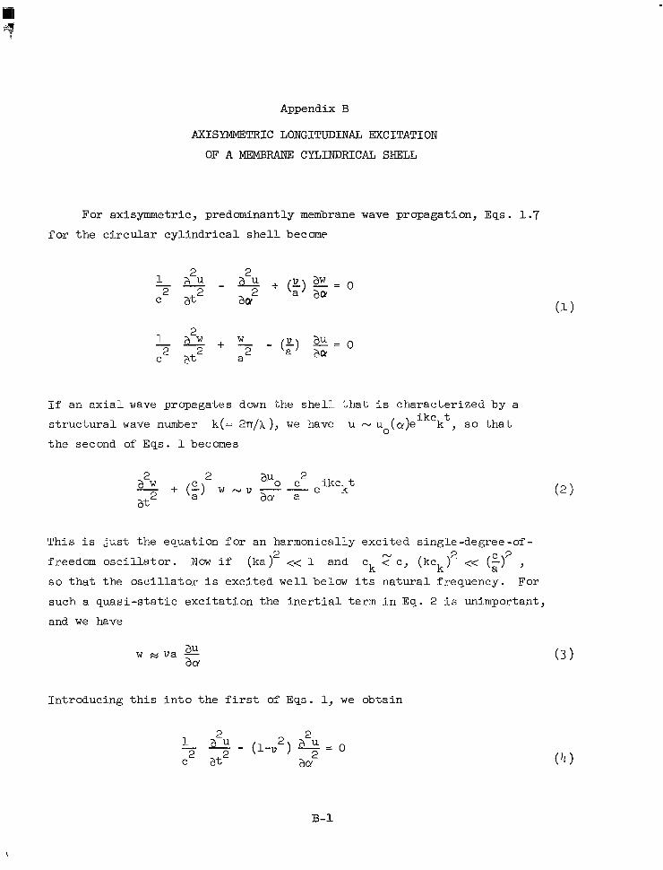
Appendix B

AXISYMMETRIC LONGITUDINAL EXCITATION

OF A MEMBRANE CYLINDRICAL SHELL

For axisymmetric, predominantly membrane wave propagation, Eqs . 1.7 f o r t h e c i r c u l a r c y l i n d r i c a l s h e l l become

If an a x i a l wave propagates down t h e s h e l l t h a t i s characterized by a

s t r u c t u r a l wave number k (= 2n/h ), we have u - u (a)eikckt, so t h a t

t h e second of Eqs. 1 becomes 0

2 2 a w a t2 aa a

C avo c 2 ikckt - + ( g ) w NU" e

This i s just the equation for an harmonically excited single-degree-of - freedom o s c i l l a t o r . NOW i f (ka) << 1 and ck < c y (kck) << (g) , s o t h a t t h e o s c i l l a t o r i s exci ted wel l below i t s natural f requency. For such a quas i - s ta t ic exc i ta t ion the iner t ia l t e rm in Eq . 2 i s unimportant,

and we have

2 N 2 c 2

w ~ v a - au aa

In t roduc ing t h i s i n to t he f i r s t of Eqs. 1, w e obtain

B-1

s o t h a t the (non-dispersive) wave t r ave l s w i th t he ba r ve loc i ty

1/2. If , however, (ka ) >> 1 and ck c , then 2

t h e i n e r t i a l term i n Eq. 2 i s dominant, and we have

In t roduc ing t h i s i n to t he f i r s t of Eqs. 1, we obtain

With u - Uoe i((-Ukt-ka) , t h i s y i e lds , s ince (ka ) >> 1, 2

so t ha t t he wave t r ave l s e s sen t i a l ly w i thou t d i spe r s ion a t t he p l a t e

v e l o c i t y e . F i n a l l y , i f ka N 1 , no s impl i f ica t ion i s possible and

the propagation i s charac te r ized by s ign i f icant d i spers ion .

We have j u s t observed tha t , fo r ax ia l ly p ropagat ing d i s turbances

with pronounced cha rac t e r i s t i c wave lengths, long wave length disturbances

[(ka) >> 13 propagate as nondispersed waves along a bar and shor t wave

length dis turbances [ (ka) >> 13 propagate as nondispersed, straight-

c res ted waves i n a n i n f i n i t e p l a t e . For general exci ta t ions, however, a

more sophis t ica ted ana lys i s i s required.

2

2

B .1 PERTURBATION TECHNIQUE

Let US write Eqs. 1 i n terms of the non-dimensional variables

u = u/a, w = w/a, 7 = ct /a A A

B-2

and then omit the circumflex notation to obtain

We now expand u and w as fol lows

subs t i t u t e i n to Eqs . 9, and equate the coef f ic ien ts of l i k e powers of

u to obtain the displacement recursion formulas

, i = 0,1,2, . . .

Considering the r ight side of each of these equations as known, we see

t h a t t h e e q u a t i o n s a r e p a r t i c u l a r l y e a s y t o s o l v e , t h e f i r s t b e i n g t h e

wave equation and the second the equation of motion f o r a simple o s c i l l a t o r .

Furthermore, satisfaction of the appl icable boundary cond i t ions a t t he

ze ro th l eve l y i e lds w ( O ) = u ( l ) = = = . . . = 0 . Thus, s ince

v2 i s general ly much smaller than unity, convergence of t h e s e r i e s of

Eqs. 10 i s rap id . We now i l l u s t r a t e t h e a p p l i c a t i o n of the per turbat ion

technique by t reat ing t.wo simple impact problems f o r a semi- inf ini te

s h e l l .

B-3

Consider an in i t ia l ly qu iescent semi- inf in i te she l l . tha t i s subjected

t o a prescr ibed longi tudinal end displacement u(0,t) = f ( T ) H ( T ) , where

H ( T ) i s the Heaviside step-function. From Eqs . 11, then,

where f ' i s the der iva t ive of f with respect to i t s a r g m e n t . 3t

We now seek u (2) (u") being zero) which, from Eqs . 11 and 12,

i s given by

The des i r ed pa r t i cu la r so lu t ion t o t h i s equa t ion i s of the form

Thus, Eqs . 13 and 14 yield

7-CY

0

The homogeneous s o l u t i o n t o E q . 13 i s of the form

r Response d i scon t inu i t i e s a r e most conveniently handled through the use of general ized funct ions.

B-4

Fina l ly , s ince u ( O ) s a t i s f i e s our boundary condition a t ~y = 0 , w e have u ' ~ ) ( O , ~ ) = 0 , which, from Eqs. 14 and 15, yie lds

Thus, from Eqs . 14, 15 and 17, we obtain

7-CY n

so tha t , from E q s . 10, 12 and 18,

0 0

AS T increases , addi t ional terms are required; for example, we w i l l

require below the addi t ion of the O ( u ) term t o the second of E q . 19. From E q . 18 and the second of E q s . 11, this term i s given by

3

where n

and from Eq. 20,

Figure 1 presents longi tudinal and radial veloci ty snapshots from

Eqs . 22 and from Refs. 13 and 1 4 f o r ? = 2 and 5. The results from

R e f . 14 were obtained by application of t he method of c h a r a c t e r i s t i c s

t o t h e membrane she l l equa t ions ; the resu l t s f rom R e f . 13 were obtained

by appl icat ion of t h e method of cha rac t e r i s t i c s t o equa t ions appropr i a t e

t o improved (Timoshenko) she l l theory . F igure 2 shows longi tudinal and

radial veloci ty snapshots f rom E q s . 22 and 23 and from Ref. 1 4 f o r t h e

r a the r l a t e t ime T = 10. We observe the s ignif icant improvement i n t h e

s o l u t i o n f o r 4 ( ~ ~ , 1 0 ) through the addition of t he O ( u 3 ) term.

Longitudinal and circumferent ia l membrane s t r e s s i n t h e c y l i n d r i c a l

she l l a re g iven by

0 = - - au yw u acu

0 9 ” W + V - aCY - au

where 0 and og are norulalized t o E / ( l - u ). Resul ts for these

quan t i t i e s i n t he fo rm of snapshots a t T = 2 and 5 appear i n F i g u r e 3 . The 0 - results from E q s . 22 and 24 include terms up t o and including

those of order u 2 , while the 0 - results from those equations per- 9

t a i n t o a s ingle O ( u ) term. The r e s u l t s from R e f . 14 p e r t a i n t o a

modal superposit ion solution of membrane theory shell equations, while

those from R e f . 13 p e r t a i n t o a method of c h a r a c t e r i s t i c s s o l u t i o n of

improved theory shel l equat ions. Figure 4 shows longi tudina l and c i r -

cumferential membrane s t r e s s snapsho t s a t T = 10. A - r e s u l t w i t h

2 CY

CY

7 % terms up t o and including those of order vJ i s shown i n t h i s

we no t i ce he re t oo t he s ign i f i can t improvement in t he so lu t ion

the addi t ion of t he O ( u 3 ) tern1 t o t h e second of Eqs. 19.

We observe in F igures 1-4 t h a t a per turbat ion solut ion of

f igu res ;

through

given

order begins t o f a i l a s 7 increases . This comes a s no surpr ise , s ince

we expect the cumulative effects of coupl ing through Poisson’s ra t io

eventua l ly to p roduce such fa i lure . It is , i n f a c t , r a t h e r s u r p r i s i n g

B-6

t h a t t h e T = 5 and 10 solut ions of Figures 1-4 are as accura te as they

are , s ince we a l so expec t to encounter convergence problems a s v T

approaches unity. Even when v 7 > 1 , however, the per turbat ion solu- 2 -

t i o n i s convergent i n t h e v i c i n i t y of the wave front. Furthermore, when

7 >> 1 , asymptotic methods may be used t o obtain solutions, as i n Ref. 33.

2

B -3 PRESCRIBED END LOAD

We now cons ider an in i t ia l ly qu iescent semi- inf in i te she l l tha t i s

excited by a prescr ibed longi tudinal end load 5 ( 0 , ~ ) = f ( 7 ) H( 7 ) . To

t r e a t t h i s problem, we use E q s . 24 t o transform Eqs. 9 i n t o t h e s e t CY

2 2 2 a OCy " 2 a OCy

aT a a aT

a a 2 ( 1 - v ) - 2 - 9 2 =

0

N O W it i s c lear tha t these equat ions l ead to per turba t ion so l ' l t ions which ~ 2-12

pred ic t t ha t t he waveeon t t r ave l s a t t he ba r ve loc i ty Cb = (1-11 ) C - Hence, ye recombine these equat ions to obtain the equivalent set

B-7

Following the same procedure used t o obtain Eqs . 11, we obtain the

s t r e s s r ecu r s ion formulas

Sa t i s f ac t ion of the boundary conditions appropriate to these equations

a t t h e z e r o t h l e v e l y i e l d s (0) - - (1) = CJ ( 2 ) = CJ ( 3 ) = . . . = 0. OCY e CY

For the prescr ibed end load C J ~ ( O , T ) = f ( 7 ) H(T) , we obtain from

Eqs. 27

Next we seek CJ ( 2 ) , which, from E q s . 27 and 28, i s given by CY

Proceeding as before , we f i n d

so t h a t , from E q s . 28 and 30

B-8

T-CY

A s increases , addi t ional terms are again required; for example, from

Eq. 30 and the second of E q s . 27, t he O ( u ) term f o r (J (CY,T) is given 3 e

by

7- CY

where F (7 ) i s given by Eq. 21 and F ' (7 ) i s the der iva t ive of F ( 7 )

with respect t o argument.

A s an example, w e consider the case of a ramp end-load; i .e ., f ( T ) = 7 . From Eqs . 31, then,

Figure 5 shows snapshots of longi tudinal and c i r cumfe ren t i a l s t r e s s

response a t T = 2 . The r e s u l t s from Ref. 14 were obtained by applica-

t i o n of t he Iiiethod of c h a r a c t e r i s t i c s t o t h e membrane shel l equat ions;

we see that they are very closely approximated by the perturbation

s o l u t i o n s a t t h i s r a t h e r e a r l y t i m e .

Before concluding this discussion, le t us br ief ly examine the argu-

ment behind the transformation of E q s . 2 5 i n t o E q s . 26, v iz ., t ha t pe r -

turbation solutions obtained from E q . 26 give c instead of c a s t he

wave f ron t ve loc i ty . Th i s i s c lear ly des i rab le i f one i s i n t e r e s t e d i n

information near the wave f ron t , bu t i s less d e s i r a b l e i f t h e e x c i t a t i o n

f ( T ) va r i e s so slowly that the shel l behaves much l i k e a bar. I n t h e

l a t t e r ca se , it i s b e t t e r t o use Eqs. 25 or, i n t h e c a s e of prescribed

end motions, the equations

b

B-9

The so lu t ions to these equat ions tha t cor respond to Eqs . 19 are

and the so lu t ions t o Eqs. 25 t h a t correspond tO Eqs. 31 a re

0 0

T* -CY

0

* 2 1/2 where T = ( 1 - u ) T = c t / a and f i s . the four th der iva t ive of f

i v b

wi th respsc t t o argument. For the examples considered above, Eqs. 35 and

36 yield responses which d i f f e r from those produced by Eqs. 19 and 31 only i n t h a t T i s replaced by T . For slowly-varying excitations,

however, Eqs. 35 and 36 should yield better solutions than Eqs. 19 and

*

B-10

B - 4 CONCLUDING REMARKS

We have seen that the per turbat ion method can provide remarkably

accura te so lu t ions for problems involving the propagation of t r ans i en t ,

axisymmetric s t r e s s waves i n e l a s t i c c y l i n d r i c a l s h e l l s . I n a d d i t i o n ,

the technique may be a p p l i e d t o a va r i e ty of r e l a t ed pr'oblems, such a s

the propagation of compressional waves i n e l a s t i c r o d s . T o i l l u s t r a t e

t h i s app l i ca t ion , we consider the Mindlin-Herrmann equations (Ref. 34)

N

where u and w are longi tudina l and radial displacements, respectively,

p and a are the rod densi ty and radius , respect ively, I and p, a re

the Lame' constants, and n and n1 are cor rec t ion fac tors on the order

of un i ty . For motions with spatial wave lengths on the order of and la rger

than the rod radius, the third term on t h e l e f t s i d e of the second of

Eqs. 37 may be neglected in favor of the term immediately preceding i t .

This yie lds a s e t of equat ions that are of the same form a s Eqs . 9, which

permits direct appl icat ion of the per turbat ion technique appl ied to Eqs. 9.

N

B - U

0.8

0.6

0.4

0.2

0

-0.2

- 0.4

t FROM Ref. 13 COINCIDENT

/ I I /

I

Figure 1. Velocity Snapshots a t 7 = 2 and 5 (Step-Velocity Excitation)

B-13

4.2

1 .o

CI 0.8 0 -= 0.6 a v

-3, 0.4 n

0 a -3

-- 0.2

0

-0.2

- 0.4

v

IC

B-14

J

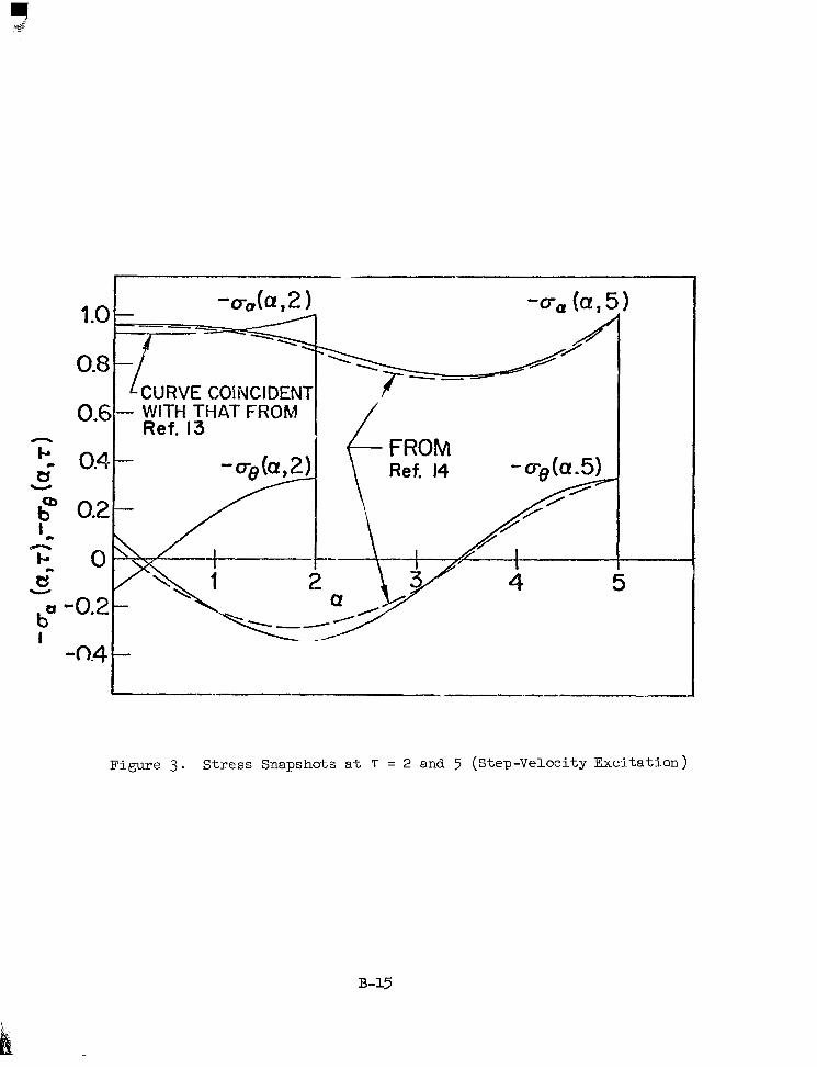
1

t Figure 3. Stress Snapshots a t T = 2 and 5 (Step-Veloci ty Exci ta t ion)

""""-

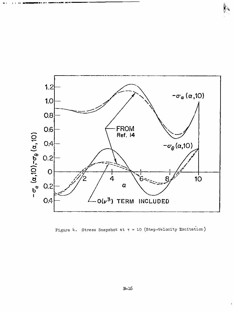
1.2-

B-16

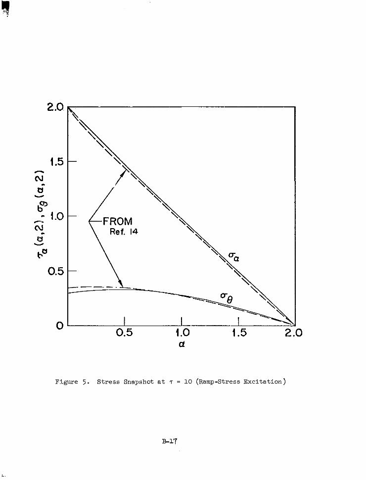
2 .o

1.5 h

cu a

U

0.5

0 0.5 4 .o d

1.5 2 .o

Figure 5 . Stress Snapshot a t T = 10 (Ramp-Stress Exc i t a t ion )

L

REFERENCES

1. S . Timoshenko .and D . H. Young, Vibration Problems in Engineering, Van Nostrand Company, I n c ., (3rbEd.]-, ,1955.

2 . J . A . Asel t ine , Transform Methods i n Linear System Analysis , McGraw - H i l l Book Company, Inc . , 1958.

-

3. A.E.H. Love, A T r e a t 1 1 Dover Publ icat ions, New York, 1926.

-~ .

4. W . Fliigge, Stresses in Shel ls , Springer-Verlag, New York, 1967.

6. J. Kempner, ' vn i f i ed Thin S h e l l Theory, I t Poly techn ica l In s t i t u t e of Brooklyn, PIBAL Report No. 566, March 1960.

7- H. Kraus, Thin Elastic Shells, John Wiley & Sons, Inc ., New York, 1967.

8. I . Mirsky and G . HerrmaK, "Nonaxially Symmetric Motions of Cy l ind r i ca l She l l s , I' J . Acoustical SOC. Am., Vol. 29, pp 1116-1123 (1957) s e e a l s o J. Acoustical SOC. Am., Vol. 31, p 250 (1959)

9. R . F . Hartung, "An Assessment of Current Capabi l i ty for Computer Analysis of She l l S t ruc tu res , " J1. Computers & Structures, Vol. 1, 1971.

10. L . H . Sobel, W . Silsby, B . G . Wrenn, "Computer User 's Manual f o r t h e STAR (Shel l Trans ien t Asymmetric Response) Code , 'I SAMSO-TR-70-240, LMsC-Do06673, Apri l 1970.

11. J. W . Leech, P. T . Hsu, E . W . Mack, "S tab i l i t y of a Fini te Difference Method for Solving Matrix Equations, 'I A I A A J. , Vol. 3 , No. 11, Nov. 1965, pp 2172-2173.

12. J . P. Raney and J . T . H m l e t t , "A Modal So lu t ion fo r Wave Propagat ion in F i n i t e S h e l l s of Revolution, I' presented a t t h e AIAA/ASME 11 th S t ruc tu res , S t r u c t u r a l Dynamics and Materials Conference, Denver, Colo., Apri l 1970.

13. P. C . Chou, "Analysis of Axisymmetrical Motions of Cy l ind r i ca l She l l s by the Method of Charac t e r i s t i c s , " AIM J., Vol. 6, No. 8, Aug. 1968, PP 1492 -1497

1 4 . S..Adham, 'kave Propagation i n E l a s t i c and E l a s t i c - P l a s t i c C y l i n d r i c a l She l l s , 'I Ph.D. Dissertation, Univ. of Southern California , 1967.

15 . J. P . Raney, P r iva t e Communication, August 1970.

R-1

16.

17.

18.

19 *

20.

21.

22.

23 -

24.

26.

27..

28.

R . W. Mortimer, P. C . Chou, J. L. Rose , "Annual Report i n Stepped and Joined Shells, " NASA Grant NGR 30-004-013, October 1969.

V. H. Kenner, W. Goldsmith, and J . L . Sackman, "Longitudinal Impact on a Hollow Cone," J. of Appl. Mech., Vol. 36, Sept . 1969, pp 445-450.

B. A. Boley and C . C . Chao, "Some Solut ions of t he Timoshenko Beam Equations, ' I J. of Appl. Mech., Vol. 22, Dec . 1955, pp 579-586.

F. S . Crawford, Jr. , Waves, McGraw-Hill Book Company, New York, 1965.

T . von Karman and M . A . Biot, Mathematlcal Methods in Engineering, McGraw-Hill Book Company, New York, 1940.

R . S . Dunhan, R . E . Nickel1 and D . C . St ickler , "Integrat ion Operators f o r a Transient Structural Response, I' proceedings of Conference on Computer Oriented Analysis of S h e l l S t r u c t u r e s , Lockheed Missi les & Space Company, Palo Alto, Calif ., August 1970.

J. W . Leech, " S t a b i l i t y of Finite Difference Equation for the Transient Response of a F l a t P l a t e , AIM J. , Vol. 3, No. 9, Sept . 1965, PP 1772 -1773 a .

G . G . 0 'Brien, M . A . Hyman, and b . Kaplan, ''A Study of the Numerical Solut ion of Pa r t i a l D i f f e ren t i a l Equa t ions , I f J. Math & Physics, Vol. 29, 1951, PP 223-251.

B . G . Wrenn, L . H . Sobel and W . S i lsby, "Nonsymmetric and Nonlinear Response of Thin Shells, 'I Lockheed Missi les & Space Company Report No. B-72-67-3, Dec . 1967.

L . Morino, J. W . Leech, and E . A . Witmer, "PETROS 2 : A New F i n i t e Difference Method and Program for the Calcu la t ion of Large Elast ic- P l a s t i c Dynamically Induced Deformations of General Thin Shells," BRL CR 12, Dec. 1969.

R . D . Mindlin, "An IntroducLion t o the Mathematical Theory of Vibrations of E l a s t i c P l a t e s , 'I U.S. Army Signal Corps Engineering Laboratories, Fo r t Monmouth, N.J., 1955.

T . L . Geers, 'hn Approximate Method for. Analyzing the Vibrations of S t i f fened P la tes and S h e l l s , " Cambridge Acoustical Associates, Inc. , Cambridge, Mass., Final Report (11) U-238-165, under contract NObs-90438, Nov. 1966.

T . L. Geers and S . A . Denenberg, "A D i g i t a l F i l t e r for Separating High- and Lm-Frequency Components of a Transient Signal, " David Taylor Model Basin Report 1795, Jan. 1964.

K . Knopp, I n f i n i t e Sequences and Series (Trans. by F. Bagemihl) , Dover Publ icat ions, New York, 1956.

R-2

30. V. V . Novozhilov and L. I . Slepian, "On Saint-Venant ' s P r i n c i p l e i n t h e Dynamics of Beams,J' PMM, Vol. 29, No. 2, 1965, pp 261-281.

31. D . A. Evensen, Monthly Progress Report NO. 10, NASA/Langley Contract NAS 1-9876, March 1971.

32. R . H. Chalmers and H . A . Gaberson, '!Modal Velocity as a Cr i t e r ion of Shock Severity," Naval Electronics Laboratory Report NEL 1682, Jan. 1970.

33. H. M. Berkowitz, "Longitudinal Impact of a Semi-Inf i n i t e E l a s t i c Cy1in.- d r i c a l S h e l l , " J. of Appl. Mech., Vol. 30, Sept . 1963, pp 347-355.

34. R. D . Mindlin and G . Herrmann, Proc . 1st U.S . Nat '1 Cong. Appl. Mech., June 1951, ASME, New York,.N.Y., 1952, pp 187-191.

NASA-Langley, 1971 - 32 CR-1885

L

R-3

ANALYSIS OF TRANSIENT, LINEAR WAVE BY THE FINITE DIFFERENCE METHOD · 2017-07-01 · ANALYSIS OF...

Documents

Transcript of ANALYSIS OF TRANSIENT, LINEAR WAVE BY THE FINITE DIFFERENCE METHOD · 2017-07-01 · ANALYSIS OF...