Analysis of the temporal electric fields in lossy ...orbit.dtu.dk/files/3813752/McAllister.pdf ·...

General rights Copyright and moral rights for the publications made accessible in the public portal are retained by the authors and/or other copyright owners and it is a condition of accessing publications that users recognise and abide by the legal requirements associated with these rights.

• Users may download and print one copy of any publication from the public portal for the purpose of private study or research. • You may not further distribute the material or use it for any profit-making activity or commercial gain • You may freely distribute the URL identifying the publication in the public portal

If you believe that this document breaches copyright please contact us providing details, and we will remove access to the work immediately and investigate your claim.

Downloaded from orbit.dtu.dk on: Aug 08, 2018

Analysis of the temporal electric fields in lossy dielectric media

McAllister, Iain Wilson; Crichton - Fratrådt, George C

Published in:IEEE Transactions on Electrical Insulation

Link to article, DOI:10.1109/14.85125

Publication date:1991

Document VersionPublisher's PDF, also known as Version of record

Link back to DTU Orbit

Citation (APA):McAllister, I. W., & Crichton, G. C. (1991). Analysis of the temporal electric fields in lossy dielectric media. IEEETransactions on Electrical Insulation, 26(3), 513-528. DOI: 10.1109/14.85125

http://dx.doi.org/10.1109/14.85125

http://orbit.dtu.dk/en/publications/analysis-of-the-temporal-electric-fields-in-lossy-dielectric-media(2382ccd0-d138-4758-9d1a-7f98b0c0962b).html

IEEE Transactions on Electrical Insulation Vol. 26 No. 3, June 1991 513

Analysis of the Temporal Electric Fields in Lossy Dielectric Media

I . W. McAllister and G. C. Crichton Physics Laboratory 11,

The Technical University of Denmark, Lyngby, Denmark

ABSTRACT The time-dependent electric fields associated with lossy dielectric media are examined. In the analysis, it is recalled that space charge, which accumulates at an interface, is an inherent feature of lossy dielectrics. This behavior can lead to en- hanced normal and tangential electric fields. The analysis illustrates that, with respect to the basic time constant E / Y , these lossy media can take a considerable time (> ~ E / Y ) to attain a steady-state condition. Time-dependent field enhancement factors are considered, and inherent surface-charge densities quantified. Thereafter, the calculation of electrostatic forces on a free, lossy dielectric particle is illustrated. An extension to the basic analysis demonstrates that, on reversal of polarity, the resultant tangential field at the interface could play a decisive role in the insulation integrity of a system. The paper concludes with a discussion of the relevance of the field aspects presented to the behavior of dielectric spacers as used in DC GIS, and introduces the importance of surface conductivity.

1. INTRODUCTION

N practice, all solid insulators are lossy dielectrics, ex- I hibiting both permittivity E and conductivity 7. The value of-y/E is often so small in comparison to the frequen- cy of the applied voltage, that the influence of the conductivity on insulation behavior can be neglected. This assumption cannot be made in relation to dc insulation, which is effectively controlled by the conductivity of the spacer material. Although Maxwell’s Treatise [l] has an entire chapter on lossy dielectrics, the significance of lossy dielectric media for dc insulation only becomes fully ap- parent following a detailed study of the overall field characteristics of the problem in question.

In the present paper, we will examine these field aspects for an insulation system consisting of two lossy media. In

particular, we will examine the fields established following polarity reversal: i.e. the fields which result from a superposition of the field due to the existing interface charge with that of the reversed applied field. In both cases our starting point is the derivation of the associated potential distributions.

2. GENERAL FIELD ASPECTS

E consider a system of two homogeneous isotropic W media a and b which possess permittivities E ~ , t h

and conductivities yn, ya, respectively. Medium b represents an uncharged inclusion embedded within medium a which occupies the remaining volume extending to infin- ity. This system of two lossy dielectrics is located in an extended uniform field.

0018-9367/91/0600-513$1.00 @ 1991IEEE

Authorized licensed use limited to: Danmarks Tekniske Informationscenter. Downloaded on November 6, 2009 at 10:03 from IEEE Xplore. Restrictions apply.

514 McAllister et al.: Temporal Electric Fields in Lossy Dielectrics

To enable general field expressions to be developed pri- or to referring to specific geometries, we will use initially generalized orthogonal coordinates U; (i = 1,2,3). The interface between media a and b is assumed to be a surface of constant u1 (= a) and hence the two remaining coordinates u 2 and u3 represent surface coordinates on the interface.

In deriving the time-varying potential solution for lossy dielectrics, we must refer t o the continuity equation

where J' is the volume current density, p the volume charge density, and t the time. _This equation express- es the r$ationship between the J field and the 5 field, where D is the electric flux density. However, to satisfy the boundary conditions a t the interface between m e d i t a and_ b , i .e. continuity of the normal components of J and D , we must express (1) in a form applicable to a surface of discontinuity. This leads to an equivalent interface continuity equation

- aU G . A J + - = O at

where U is the surface charge density. _The term 5 . A f represents the interface divergence of J and, with reference to the present analysis, can be expressed as

- + -

5 . A f = n ' . ( J a - Jb) (3)

G is a unit vector normal to the interface in the direction b to a . This orientation is also associated with increasing values of ul, so that qa 2 ulb. Similarly, with respect t o the fi field, we have

U = 5 . (fia - &) (4)

As both .f and are+ propoftionaf to the electric field strength E, i.e. J = yE and D = &E, (2) can be rewritten in terms of E'. In addition, at the interface (u1 = a) the normal component of E' is El, where El is given by

(5)

9 represents the potential in question and 911 is the relevant metric coefficient with

Consequently, if 9n(u1, uz, u3, t ) and 9 b ( u 1 , u 2 , u3, t ) denote the potential distributions in media a and b , respectively, then the interface continuity equation for the

surface (ul = a) may be expressed in terms of generalized coordinates as

This expression represents the general boundary condition t o be fulfilled by and 9b a t the interface (111 = a).

The other boundary condition to be fulfilled a t the interface is of coyrse the continuity of the tangential component of the E field across the interface. This condition is equivalent to the equality of the potentials a t the interface, i.e., for u1 = a, we must have

@a(% u2, u3, t ) = %(a, 212, u3, t ) (8)

3. POTENTIAL DISTRIBUTION FOR AN

APPLIED DC FIELD

3.1 GENERAL ANALYSIS

N the dc steady state ( t -+ CO), the potential distribu- I tion will be independent of time and will be controlled by the conductivities of the media, whereas a t time zero, the system permittivities will determine the potential distribution. These characteristics of the potential distribution in the two media can be accounted for by assuming that the potential function 9 can be expressed as

@ ( u l , ~ , u 3 , t ) = [ p c ( u l r ~ u 3 ) - ~ 7 ( u l , W , u 3 ) ] T ( t )

-k 'Pr(ulr u 2 , u 3 )

(9) where pE and pr are the potential functions associated with the system permittivity and the system conductivity, respectively, and as such must be solutions of Laplace's equation. On the basis of pE and p7, the function T( t ) , which represents the temporal variation of 9, is considered to be normalized such that T(0) = 1 and in addition we require that as t -+ 00, T ( t ) -+ 0.

By expressing 9 in the above manner, we have imple- mented the first step in applying the separation of variables method. A further assumption of this method is that , with reference to the problems under discussion, the p function is simply separable [2], i.e. 'p can be expressed as

p(ul, 2121 213) = u(211)V(uZ)w(u3) (10) For any coordinate system, the necessary and sufficient conditions to be satisfied with respect to the separability of Laplace's equation are discussed in Moon and Spencer PI.


IEEE !l'ransactions on Electrical Insulation Vol. 26 No. 3, June 1991 515

With reference to (9), the potential distributions in the which attains a steady-state value, c,, as t -+ CO. If Yb = 0, i.e. zero conduction in medium b, coo. can be obtained from (18). Similarly with (19) for 7, = 0. Furthermore, it should be noted that the polarity of c is determined not only by the applied voltage but also by the condition

two media may be expressed as

(I1)

(12)

an = ( v a c - p n y ) T + (Pay

ab = ('Pbc - 'Pb-y)T + (Pbr At the interface u1 = a, the potential-equality boundary condition must be fulfilled by both the (P, and the vr originally. Thus 9, and will fulfill this condition automatically. Inserting the above expressions for 9, and @b into (7) enables the interface continuity equation for the present class of problems to be derived. Taking ac-

Finally, (18) and (19) also provide confirmation of the analysis in [3] which shows that, for = 7b/~r,, there is no accumulation of charge a t the interface.

count of the boundary conditions which the yE and the vv must in turn fulfill, we can obtain for u1 = a 3.3 APPLICATION T O A SPHERICAL

INCLUSION

This expression represents one form of the boundary condition to be fulfille_d by @,+and % a t the interface. Fur- ther, owing to the D, and J, boundary relationships, (13) can be re-expressed in different ways.

To utilize the above general analysis, we consider medium b to be a sphere of radius R. Hence with respect to spherical coordinates r , 8, $ we have u1 = r , 212 = 8, 213 = $, 911 = 1 and 922 = r2 [4]. The applied field EA is oriented in the negative z direction so that the undistorted applied potential is EATcos8, i .e., the oy plane is at zero potential, and EA is applied at time zero,

As each Of the 'P derivatives is independent o f t , it is evident that (13) can be written as

with

G+AT=O dt

The general solution for (14) is

(14) From the potential solution for ideal dielectrics and field EA given in standard textbooks [3,5], we have for medium a

1 + E a r c o s 8 (21) 2 ~ n r

(15)

T = Cexp(-At) (16) and for medium b

where C is a constant. On this occasion we take C = 1.

3.2 INTERFACE CHARGE DENSITY

The field continuity boundary conditions a t the interface lead to an important feature of lossy dielectrics, viz. the existence of a surface charge density a t the interface [l , 31. This feature follows directly from (3) and (4), which together with (5) enables this interface charge density 0 to be expressed, with respect to the present analysis, as

(17)

Substituting for 9, and @ b and using the fie and 51 relationships enables ~7 to be expressed either as

To obtain the equivalent conductivity potential solutions, E is simply replaced by 7. Consequently for medium a we

and

(24)

for medium b. Hence upon substitution for '.$be and '.$by

into (15) we obtain for r = R

(25)

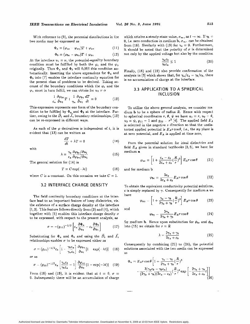
Consequently by combining (21) to (24), the potential solutions associated with the two media can be expressed as

or as -

From (18) and (19), it is evident that a t t = 0, 0 = 0. Subsequently there will be a n accumulation of charge



and

whilst from (18) and (24) the corresponding interface charge density is

3.0 1 m

2.6

2.2

1.8 . . We will now examine the relevance of this solution for two different situations.

g Lo 1L

E, = E,

2 6 8 10 10

t/Tb 0

Figure 2. Temporal variation of the field enhancement factor associated with a lossy-dielectric protrusion (yo = 0 , e,, = e,,). €,b is the relative permittivity of the protrusion material.

Figure 1. Temporal variation of the field strength in the void (yb = 0 , E b = e,,). E,,, is the relative permittivity of the bulk medium.

3.3.1 GASEOUS VOID

One of the principal causes of electrical failure of solid insulation follows from the effects of partial discharges which occur in the gaseous voids within the material. Apart from gas pressure, the occurrence of such discharges is effectively governed by the field strength attained in the void. In particular by the field along the void axis which represents the longest discharge path length in the field direction. For the void we will consider 7 b = 0 and &b = while r cos6 = z. Hence with reference to (27), the potential distribution in the void is given by

where r, = cO/ya and E, is used to denote the relative permittivity. By expressing the potential in this manner, it is evident that @ b is a linear function 2f the z coordinate alone. This feature implies that the E field in the void is uniform and oriented in the same direction (negative z direction) as the applied field EA. Hence the axial field strength Ebz in the void is

exp [&(;)]] (30)

The variation of Ebz with t for different values of is shown in Figure 1, which indicates tha t , with respect to the time constant T,, it takes a considerable time ( t > 57,) to establish the steady-state value of 1 .5E~. Al- though the permittivity of the bulk medium influences the time to attain this condition, its more significant influence is upon the initial value of Eaz. From (30) and Figure 1 it can be readily confirmed that the maximum increase in Eg, from its initial value can not exceed 50%.

From (26) we have for the bulk medium

From this expression it can be deduced that the radial


IEEE Transactions on Electrical Insulation Vol. 26 No. 3, June 1991

- component of E,, E,, is given by

R E,, = -Ea cos 8 [l - ( ,)3

from which it is evident that , a s E,, > 1, IE,r/EAl is alweys < 1, and that, as t -+ 00, the normal component of E, a t the interface tends to zero. This feature implies that a conduction steady state has been attained in medium a, while an electrostatic steady state exists in medium b.

The other field parameter of interest is the tangential field Et a t the interface. In the present case Et is given bv

( 3 3 )

For the void situation, it is readily shown that

1 -2

( 3 4 ) A comparison of ( 3 0 ) and ( 3 4 ) indicates that Et is identical in form to Ebs, apart from the sinusoidal variation around the void wall. The temporal behavior is identical.

0 2

2 6 8 10 0 O ,I-

<I L a

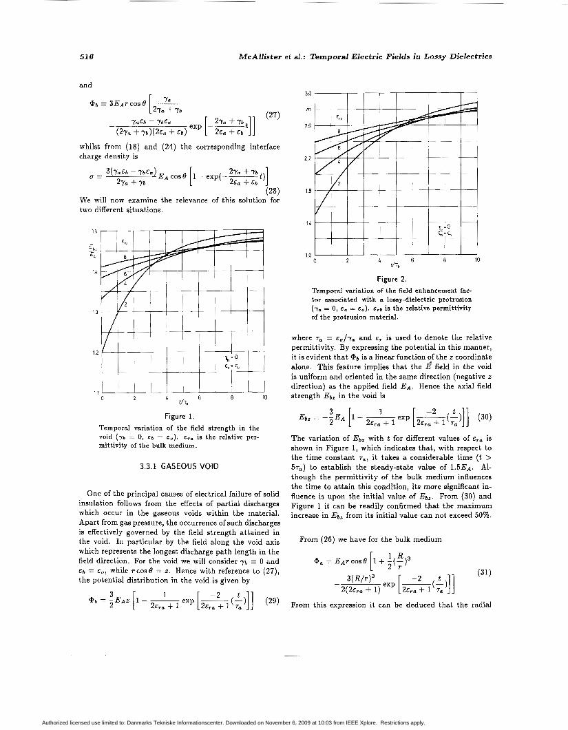
Figure 3. Temporal variation of the charge accumulation at the void interface ( 'yb = 0 , E b = E " ) . is the relative permittivity of the bulk medium.

3.3.2 LOSSY DIELECTRIC PROTRUSION IN A GASEOUS MEDIUM

Owing to the symmetry of the potential field, the zy

517

'd = o 'd,=o

Figure 4. Relationship between the polarity of the interface charge and the direction of the normal field component at the interface. (a) Void situation, (b) protrusion situation.

plane (8 = 7r /2) is an equipotential surface a t zero potential, and hence ( 2 6 ) and (27) also represent the potentia1 solution for a hemispherical inclusion on a plane conduc- tor. If 7, = 0 and E, = E ~ , the system geometry degener- ates t o a lossy dielectric hemispherical protrusion. Under such conditions, the solutions for 9, and a b reduce to

where = E o / 7 b . Because the gaseous medium will be dielectrically weaker than the protrusion, we will begin with an examination of the axial field strength E,, in the gas. Along the +z axis, 8 = 0 and hence after differentiating ( 3 5 ) we can deduce that

The increase in field strength in the gas due to the pro: trusion can be quantified in terms of a field enhancement factor m which is defined as

( 3 8 )

with m 2 1. E,,, is obtained from ( 3 7 ) for R / r = 1 and hence m can be expressed as

The variation of this parameter with time for several values of &,b is illustrated in Figure 2. I t is evident that , with reference to 'Tb, a time in excess of 10Tb is required to achieve the steady-state condition.



With respect to the protrusion, it is clear from ( 3 6 ) that

As for t + 00 Eaz + 0.

> 1, then a t t = 0, IEbl/EAI is always < 1, while

With reference to Et, it can be shown that, for the protrusion, we have

from which it is clear that , as t ++ 00, Et + 0. Such a feature taken together with the Eb behavior implies that an electrostatic steady state has been achieved in medium a , while the hemispherical interface is an equipotential surface.

2 5

F, IT E o R2 €1

2 0

15

10

Figure 5. Temporal variation of the electrostatic force on a lossy dielectric particle (7, = 0, e, = eo). €TI, is the relative permittivity of the particle material.

3.3.3 VOID/PROTRUSION INTERFACE CHARGE DEN SIT1 ES

From (28), i t is readily deduced that for the void

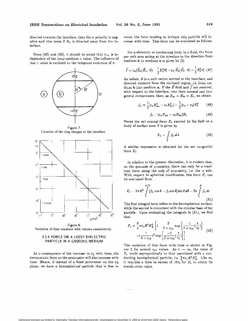
Figure 6. Relation between the ring charge geometry and the spherical coordinate system.

than U,, equal values. Each respective rate is significantly reduced by an increase in the relative permittivity of the medium in question, see Figure 3 .

For the situations presently under discussion, the polarity of U can-be predicted if we examine the normal component of E , E, at the interface. As E, -+ 0 in the lossy medium as t + 00 we need only consider E, in the gaseous medium.

With reference t o the spherical geometry, E,is given by

(44) a+ E n - a r l r = R

From (29) i t is readily shown that for the void we have

-2

(45) 3 -2 t

U,, = -E,EACOSO 2 [ l - e x p [-(-)I] 2% + 1 7, (42)

while for the protrusion we have

Apart from the obvious differences of polarity and magnitude, U,, attains a steady-state condition at a faster rate

\ ,

Similarly from (35), we obtain for the protrusion situation

(46) The relevance of E , in the gaseous medium with respect t o the polarity U is indicated in Figure 4; i.e., if E, is



directed towards the interface, then the U polarity is negative and vice-versa if En is directed away from the in- t er face.

From (42) and (43), it should be noted that um is independent of the lossy-medium y value. The influence of this y value is confined to the temporal evolution of U .

Figure 7. Location of the ring charges a t the interface.

10 ' 1 1 I 1 I I

ld8 10' 1d6 10" It;" l$ 1d2 i/(S",

Figure 8. Variation of time constant with volume conductivity.

3.3.4 FORCE ON A LOSSY DIELECTRIC PARTICLE IN A GASEOUS M E D I U M

As a consequence of the increase in U,, with time, the electrostatic force on the protrusion will also increase with time. Hence, if instead of a fixed protrusion on the zy plane, we have a hemispherical particle that is free to

move, the force tending to levitate this particle will increase with time. This force can be evaluated as follows.

For a dielectric or conducting body in a fluid, the force per unit area acting a t the interface in the direction from medium b t o medium a is given by [5]

1 1 2 2 f = [za( za . Z) - - EXG] - ~b[l?b( ,?& . Z) - - EiG] (47)

As before, 6 is a unit vector normal to the interface, and directed outward from the encl2sed region,j.e. from medium b into medium a. If the E field and f are resolved, with respect to the interface, into their normal and tangential components, then, as Eat = Eat = Et , we obtain

1 1 2 f n = j [ E a E X n - &bEin] - - [ E , - E ~ ] E ; (48)

f t [ ~ a E a n - &bE~n]Et (49)

Hence the net normal force Fn exerted by the field on a body of surface area S is given by

(50) S

A similar expression is obtained for the net tangential force Ft.

In relation to the present discussion, it is evident that , on the grounds of symmetry, there can only be a resultant force along the axis of symmetry, i.e. the z axis. With respect to spherical coordinates, this force F, can be evaluated from

X I 2 R

F, = 2xR2 / [fn cos e - f t sin e] sin e de - 2a / fn dr 0 0

(51) The first integral term refers t o the hemispherical surface, while the second is concerned with the circular base of the particle. Upon evaluating the integrals in ( 5 1 ) , we find that

The variation of this force with time is shown in Fig- ure 5 for several &sh values. As t -+ w, the value of F, tends asymptotically to that associated with a conducting hemispherical particle, i.e. : R2 E;. Like m, it requires a time in excess of l O q , for F, to attain its steady-state value.



4. POTENTIAL for which the relevant solution is

Dl STRl B UTION FOLLOW I N G T = exp( -pi) (56)

(57)

POLARITY REVERSAL with ?'a* - ? ' b e

0 = i%ao &3?= LTHOUGH the applied field can be removed and a field Ea alll &b au,

Because the interface charge distribution is axially sym-

Laplace's equation associated with spherical coordinates,

A of the opposite polarity applied following a short in- terval of time, the configuration of the interface charge density does not immediately reflect this change in

attain a steady-state configuration, so will it take a considerable time to disperse. Consequently, immediately the appropriate for and pba are [41

(9,) will be the superposition of the new applied field pau = An(R/r)n+lPn(cosO), r 2 R (58)

larity. Just as this charge takes a considerable time to metric, then, with respect to the genera' Of

following polarity reversal, the effective field distribution

To quantify the effects of polarity reversal, we will again

W

(Go) and the space-charge field a,, i.e. Qi, = Go + 9,. n=O

00

refer to a spherical inclusion in the bulk medium. p b , = An(r/R)"Pn(c0s8), r < R (59) n = O

Hence, of opposite Polarity, the Potential dis- where Pn(cos 0) is a Legendre polynomial. At the inter- tribution of the new applied field will be the same as that derived previously in Section 3.3, i .e. @,o = -a, and @bo = - @ b . Consequently only the potential distributions associated with the interface charge density remain to be derived. This will be undertaken in the following Sections.

face (. = R), pan and pba fulfill the potential-equality condition automatically.

Upon differentiating (58) and (59), and on this occasion inserting into (55), we can deduce that, for = R,

4.1 GENERAL ANALYSIS FOR A

The general potential solutions associated with the two media are thus

',, =

CHARGE SOURCE AT AN INTERFACE

(n $. I)?', -k n?'b

(n + I)&, + neb (61)

[

[

Owing to the nature of the field source (a), the conductivity of the media and the geometry of the system, a steady-state conduction field cannot exist. Consequent-

" R An(~)n+ lPn(CoSe) exp - n = O

t1 (n + I)?', + n?'b

(n + I)&, + n E b

(62)

ly, we assume that the potential distributions in the two

@ao(ui1 ~ z , % l t ) = 4aa(~i, W , ~ 3 ) T ( t ) (53)

00

media can be expressed as @bo = ~ A , ( ~ ) " P , ( c o s B ) e x p - R

n = O

To obtain A, it is necessary to derive paa and pau for the initial charge distribution at the interface.

and

If T is normalized so that T(0) = 1, then pa,, and %a(%, %,743, t ) = d b o ( U i 1 Uzl ~ 3 ) T ( t ) (54)

represent the time-zero potential distributions, i.e. those associated with the system permittivity, and they must therefore be solutions of Laplace's equation. In addition, a t the interface u1 = CY, the potential functions and ' b o , must fulfill both the continuity Equation (7) and the potential-equality condition (8).

4.2 INITIAL POTENTIAL D IST RI B U TI 0 N S FO R I N T ER FACE

CHARGE DISTRIBUTION

To determine the potential of a spherical shell of charge, we begin with the potential of an isolated elemental ring -

Consequently if we proceed as in Section 3.1 and sub- charge dq. If the ring is located a t a radial distance s from the coordinate origin, see Figure 6, then the potential of this elemental charge distribution is given by [6,7]

stitute for a,, and in (7), we obtain for '111 = a



if either r > s or r = s and 8 # p. Alternately,

if r < s or r = s and 8 # p, where p is the polar angle subtended by the ring charge. If now this ring charge is located a t the interface between the two media, then by taking account of the boundary conditions a t the interface, the potential in the two media can be shown to be with s = R

m

( 6 5 ) (R/r)"+l

dq 2 n + 1 d v a = -

47rR ( n + 1 ) ~ ~ + no, n=O

and

P, (cos p ) P, (cos e)

To take account of the inherent symmetry of the interface charge density, a second ring charge -dq subtending a polar angle of (7r-p) is introduced, see Figure 7 . By em- ploying the principle of superposition, we can obtain the relevant solutions for d v , and dpb by simply adding two solutions of the type given in ( 6 5 ) and ( 6 6 ) for dq. With -dq as the source, P,(cos p ) is replaced by Pn(cos[7r-p]). However, as

P,(cosp) - P,(-cosp) = 0 ( 6 7 )

for n even, while for n odd we have

P,(cosp) - P,(-cosp) = 2P,(cosp) ( 6 8 )

we can express the potentials in a more elegant form by replacing n by 2 n + 1. This substitution leads to

The subscript 0 indicates that these potential functions relate to a zero net charge condition at the interface. By integrating the elemental potential functions over the spherical surface we can obtain the required solutions for Pau and vbn.

From Figure 7 , it can be deduced readily that the elemental ring charge is related to the interface charge density by

On substitution for dq into the d v o expressions, we find that the relevant integrals reduce in effect to

dq = 27rR2a(p) sin p d p ( 7 1 )

1 = J a ( p ) sin ppzn+l(cos p ) d p ( 7 2 ) 0

Prior t o polarity reversal, the system was assumed to be in a steady state and thus the interface charge is the value of CT in ( 2 8 ) as t -+ 00. Thus, with respect to I , we have

Inserting this expression into ( 7 2 ) and using the recur- rence relationships obeyed by Legendre polynomials, we find that, for n 2 1,

cos p sin pPZ,+l(cos p ) d p = 0 ( 7 4 ) ?' whereas

( 7 5 ) 1

cos psin pPz,+1(cos p ) d p = - 3

for n = 0

Consequently as only the n = 0 term in the summation need be retained, the initial potential distributions associated with the interface charge distribution are simply

vaa represents a dipole potential, while is aJinear function of the z coordinate, implying that the E field in medium b is uniform. This linearity was exhibited previously by and vbr .

4.3 EFFECTIVE POTENTIAL DlSTRlB UTlON

The effective potential distributions in the two media a and b are, respectively,

@a, = @Go + @a, and

@be = @bo + a b n

A$ the undistorted potential is now -EAT cos 8, ( 2 6 ) and ( 2 7 ) represent --aa(, and -@bo, respectively.

( 7 8 )

( 7 9 )



On the basis of the change in index (n) employed to derive pan and pha, it is necessary to replace n in (60) with 2n + 1 to obtain &(n), and then set n = 0. In this way we discover that o"(0) = A, ( 2 5 ) . Thus, with respect to (61) and ( 6 2 ) , we can obtain @,, and @ha from (76), (77) and ( 2 5 ) . Consequently upon combining the various potential expressions we arrive a t

As both 9," and @ h n are exponentially decaying potentials, we see from (80) and (81) that the effect of polarity reversal is to double the magnitude of the transient potential component. Consequently as this component will have its maximum influence a t the instant of polarity reversal, we will concentrate on this aspect in the remainder of the present discussion, and proceed to examine the two situations of interest.

4.3 .1 GASEOUS VOID

Upon substituting for Yh and E h , we find that the potential functions of interest reduce to

and

where as before z = r cose.

By inspection, the axial field strength E b e Z in the is given by

2 -2 exp [ ""(31 I

while the radial field component E,,, in the bulk material can be readily shown to be

A comparison of ( 8 4 ) with (30) indicates that , as the magnitude of the transient term is doubled, the field strength in the void is effectively reduced following polarity reversal; Ehes < Ehoz. In contrast from a comparison of ( 8 5 ) with (32), we see that , as E,,, > E,, the radial field strength in the bulk is effectively increased initially. However this increase is only significant for E,, < 2.5, as only then is JE,,,/EA) > 1.

With respect to the tangential field strength Et, a t the void wall, we can deduce from either ( 8 2 ) or (83) that Et, is given by

2 -2

( 8 6 ) from which i t is evident that , like Eho, Et, will also undergo an effective reduction initially.

4.3.2 LOSSY DIELECTRIC PROTRUSION IN A GASEOUS MEDIUM

For this situation, the relevant potential functions are

From (87), it can be deduced that the axial component of the electric field E,,, in the gaseous medium is given by

( 8 9 ) By comparing (89) and (37) it is evident that the axial field strength effectively undergoes a reduction following polarity reversal; E,,, < E,,, .

Within the protrusion, the axial field strength is uniform, viz.

This expression indicates an initial doubling of Eh following polarity reversal; Ehez = 2EhOz. Similarly the interface tangential field can be shown to be given by

and like Eh, Et undergoes an initial doubling upon polarity reversal owing to the existence of the interface charges;



E t , = 2Et,. For the present interface geometry, these increases are only of significance for & l b < 4.

g = o

Figure 9. Relation between the electric field components following polarity reversal. (a ) void situation, (b) protrusion situation.

@ = V I

cp =O I

@ =O I Figure 10.

Geometry of spacer with inserts and the associated field distributions. (a ) single insert, (b) double insert.

5. DISCUSSION

5.1 T H E PRESENT ANALYSIS

5.1.1 GENERAL APPROACH

H E solution of lossy dielectric field problems is achiev- T ed through the continuity equation. For homoge-

Figure 11. Orientation of the normal field in the gas a t the spacer surface for negative dc. (a) single insert, (b) double insert.

10

0

-1 0

-2 0

I 1 I

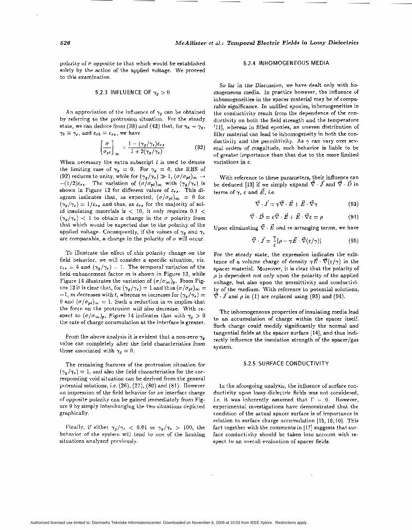
11

Figure 12. Influence of the conductivity ratio (yg/ya) on the steady-state interface charge with respect to the protrusion situation.

10

neous media, this equation reduces in effect to an associated interface continuity equation. This latter equation then serves as the boundary condition to be fulfilled a t the interfaces in question by the potentials in the bounding media. The use of this boundary condition is illustrated with reference to a particular class of boundary value problems involving an inclusion embedded in the bulk medium.

To develop a transient potential solution, it is advan- tageous to consider firstly the geometry and properties of the media, and the nature of the field source. Such an assessment enables the form of the complete potential



30

m

2 6

2 2

18

1 L

i n 10

I V

0 2 6 8 t/TS

Figure 13. Influence of 7s > 0: Temporal variation of the field enhancement factor m for a lossy dielectric protrusion, r. = 6,/yI.

10

0 8

0 6

OL

02

0 0 2 L 6 8 10

t/T,

Figure 14. Influence of yp > 0: Temporal variation of the charge accumulation at the protrusion interface, 7. = E , / 7 , .

solution to be envisaged. As shown in Sections 3.1 and 4.1, it is possible, on the basis of such an assessment, to make viable assumptions concerning the general potential solutions. Thereafter, by using the interface bound-

ary condition, the temporal variation of these potentials may be deduced.

With the general analysis, expressions for the space charge which inherently accumulates at the interface between two media have been derived. From these expressions, it is evident that the polarity of this interface charge is not determined solely by the polarity of the applied voltage, but is also influenced by the conductivities and permittivities of the bounding media.

5.1.2 LIMITING SITUATIONS

The theory has been applied to the case of a spherical inclusion, and, through a detailed examination of the field characteristics associated with the two limiting situations ya = 0 or ' y b = 0, a broad coverage of lossy-dielectric field behavior has been elucidated.

In each situation, it has been shown that, with respect to the relevant time constant T , the system takes a considerable time to attain a steady state. As we define r = ~ ~ / y , a knowledge of the appropriate y value is necessary to enable the timescale under discussion to be quantified. However, as the cautionary comment in Kaye and Laby [8] indicates, y values for insulating materials are very uncertain: e.g., in the literature, y for epoxies lie in the range to 1 O - l ' S m- l . The significance of such a y range on T can be readily appreciated from Figure 8. On the basis of Figures 3 and 8, it may be concluded that for insulating materials (y < S m-l , E~ - 4) the initial charge accumulation is liable to be on a time scale of < 5 h, while the steady-state condition could take up to several days (> 100 h) to be established. Such charging behavior is reported in [lo].

In the process of attaining this condition, the gaseous medium (defined by y = 0) is found to be subjected to an E' field which increases with time, see Figures 1, 2 and 5 , such that, in the steady state, the stress level reached is significantly greater than the initial level, which was controlled solely by the system permittivities.

The accumulation of charge a t an interface is brought about by the presence of an electric field. On reversal of the applied-voltage polarity, a completely new field configuration will be established. Depending on the polarity configuration of CT, the effective field magnitude may either be the sum or difference of the two component fields; viz. the one associated with U and the other due to the applied voltage. The former condition represents an enhancement of the applied field, while the latter brings about a reduction.



With respect to the two limiting situations studied, an appreciation of the above features can be gained from Figure 9. As may be readily deduced, the applied field in the gaseous medium is seen effectively to undergo a reduction following polarity reversal. However, should the accumulated charge distribution oppose in effect the original applied-field, see Figure 9b, then upon polarity reversal, the transient tangential field a t the spherical interface initially doubles. Depending on the overall geometry in question, the occurrence of such a n increase in the tangential field could promote surface flashover; for example breakdown along a spacer surface in a DC GIs.

Although the present study was undertaken with respect t o a spherical inclusion in a bulk medium, the same general field characteristics will be exhibited by other inclusion geometries. In addition, numerical da t a are not anticipated to differ significantly from the values obtained in the spherical case, and thus conclusions will remain un- altered.

present study to such investigations, we will confine our comments to right circular-cylindrical spacers with inserts. sufficient information exists in the literature de- scribing the electric fields associated with such spacers to allow specific comments to be made on their characteristics. In the following discussion, we will adopt the subscripts s and g in relation to the solid spacer and the gas, respectively.

The relevant spacer geometries are shown in Figure 10, along with the field lines of the vE distribution. From the field plots, it is evident that , with a single insert, a field line which intersects the spacer surface does so only once. For the double-insert spacer, the field-line intersec- tion occurs twice. The actual electric field distributions along such spacer surfaces are illustrated in [lo], and these indicate that the maximum normal field in the gas a t the interface is located approximately coincident with the end of the insert.

5.2.2 CHARGE POLARITY 5.1.3 MAGNITUDE OF (T,

On attaining the the steady-state condition, we find that (U,[ - E ~ E A , see (42) and (43). For SFG at 0.2 MPa, a typical E value would be 5 kV/mm, from which we obtain IC, I - 45 pC/m2. This value is of the same order of magnitude as the U values reported in the literature, e.g. see [9,10]. Hence we cannot disregard the fact that the accumulation of such charge levels a t spacer surfaces could arise as a direct consequence of the spacer behaving as a lossy dielectric: i.e. the conductivity of the spacer material should not be treated unreservedly as zero.

5.2 DC GIS SPACERS

5.2.1 GENERAL ASPECTS

Invariably the geometry of practical spacers is such that the surfaces of these do not conform t o any of the surfaces generated by the separable coordinate systems [4]. Con- sequently the separation of variables method employed in the present analysis cannot be used t o determine the fields associated with practical spacer designs. Neverthe- less some of the field characteristics of such spacers can be inferred from the present study.

Throughout the 1980’s many experimental investigations have been concerned with the accumulation of charge on dc spacers following the application of the system voltage (we are not referring t o studies in which charge is artificially deposited). In discussing the relevance of the

Fujinami et al. [ lo] reported on measurements in SFG a t -200 kV, and with this voltage polarity E,, will be oriented as shown in Figure 11. Consequently, on the basis of the discussion in Section 3.3.3, we would anticipate charge maxima of negative polarity t o accrue a t A and B, see Figure 11, while a t C the maximum accumulation of positive charge would occur. In fact Fujinami et al. [lo] recorded positive charge a t A and B, and negative charge a t C, i.e. the directly opposite polarity to that predicted by the initial analysis. In [lo], the explanation provided is that charge in the gas accumulates a t the spacer surface until E,, = 0. The maximum attainable level of charge is then obtained by setting U, = - E , E,,. This procedure, which gives reasonable agreement between calculated and measured (T values, is in contrast to the lossy dielectric approach which leads naturally to the steady-state condition of E,, = 0, such that U, = coEgn, and thus a change in (T polarity will arise.

A possible explanation for this behavior lies in the fact that , with respect to lossy dielectrics, the polarity of (T is not controlled uniquely by the applied voltage, but also by the permittivities and conductivities of the media, see Section 3.2. Until now we have treated y, = 0. If, however, y, < S m - l , see [ll], then the fact that all gases exhibit a very low inherent conductivity, can no longer be ignored. Such a background conductivity was invoked by Gaertner et al. in a study of the decay of surface charge [12]. To establish the influence of a non-zero y, on the spacer charging process, it is necessary to examine the values of the ratio (y,/y,) which provide a change in the



polarity of D opposite to that which would be established solely by the action of the applied voltage. We proceed to this examination.

5.2.3 INFLUENCE OF ys > 0

An appreciation of the influence of ys can be obtained by referring to the protrusion situation. For the steady state, we can deduce from (28) and (43) that, for ya ys, ' yb z ys, and &rb E , , , we have

When necessary the extra subscript 1 is used to denote the limiting case of yg = 0. For (̂s = 0, the RHS of (92) reduces to unity, while for (yg/y,) >> 1, ( U / O ~ Z ) ~ -+

- ( 1 / 2 ) ~ ~ # . The variation of ( c r / c ~ ~ p l ) ~ with (yg/y8) is shown in Figure 12 for different values of 6,". This di- agram indicates tha t , as expected, ( u / u ~ ~ ) ~ = 0 for (ys/y , , ) = 1 / ~ ~ , and thus, as E ~ , for the majority of solid insulating materials is < 10, it only requires 0.1 < (yg/yd) < 1 to obtain a change in the D polarity from that which would be expected due to the polarity of the applied voltage. Consequently, if the values of yg and y, are comparable, a change in the polarity of c~ will occur.

To illustrate the effect of this polarity change on the field behavior, we will consider a specific situation, viz. E,# = 4 and (ys/y , , ) = 1. The temporal variation of the field enhancement factor m is shown in Figure 13, while Figure 14 illustrates the variation of ( u / u ~ ) ~ . From Fig- ure 13 it is clear tha t , for (ys/y,) = 1 and thus ( u / u ~ ~ ) ~ = -1, m decreases with t , whereas m increases for (ys/yb) = 0 and ( U / ~ T ~ I ) ~ = 1. Such a reduction in m implies that the force on the protrusion will also decrease. With respect to (c/cm),,, Figure 14 indicates that with yg > 0 the rate of charge accumulation a t the interface is greater.

From the above analysis it is evident that a non-zero ys value can completely alter the field characteristics from those associated with ys = 0.

The remaining features of the protrusion situation for (ys/y,) = 1, and also the field Characteristics for the corresponding void situation can be derived from the general potential solutions, i.e. (26), (27), (80) and (81). However an impression of the field behavior for an interface charge of opposite polarity can be gained immediately from Fig- ure 9 by simply interchanging the two situations depicted graphically.

Finally, if either ys/y8 < 0.01 or ys/ys > 100, the behavior of the system will tend to one of the limiting situations analyzed previously.

5.2.4 INHOMOGENEOUS MEDIA

So far in the Discussion, we have dealt only with homogeneous media. In practice however, the influence of inhomogeneities in the spacer material may be of comparable significance. In unfilled epoxies, inhomogeneities in the conductivity result from the dependence of the conductivity on both the field strength and the temperature [ll], whereas in filled epoxies, an uneven distribution of filler material can lead to inhomogeneity in both the conductivity and the permittivity. As y can vary over several orders of magnitude, such behavior is liable to be of greater importance than that due to the more limited variations in E .

With reference to these parameters, !heif. influe_nce_can be deduced [13] if we simply expand V . J and V . D in terms of y, E and E , i.e.

+

e . f= ye .z+ 2.37 (93)

(94) 4 4

Upon eliminating V . E and re-arranging terms, we have

(95)

For the steady state, the expression iniicetes the existence of a volume charge of density y E . V ( E / ~ ) in the spacer material. Moreover, it is clear that the polarity of p is dependent not only upon the polarity of the applied voltage, but also upon the permittivity and conductivi- t,y of the medium. With reference to potential solutions, V . f and p in (1) are replaced using (93) and (94).

The inhomogeneous properties of insulating media lead to an accumulation of charge within the spacer itself. Such charge could modify significantly the normal and tangential fields a t the spacer surface [14], and thus indi- rectly influence the insulation strength of the spacer/gas system.

5.2.5 SURFACE CONDUCTIVITY

In the aforegoing analysis, the influence of surface conductivity upon lossy-dielectric fields was not considered, i.e. it was inherently assumed that r = 0. However, experimental investigations have demonstrated that the condition of the actual spacer surface is of importance in relation to surface charge accumulation [15,16,10]. This fact together with the comments in [17] suggests that surface conductivity should be taken into account with respect to an overall evaluation of spacer fields.


IEEE !lkansactions on Electrical Insulation Vol. 26 No. 3, June 1991 527

If I’ > 0, then it becomes necessary to modify (2) such REFERENCES that the existence of a surface current density l? is accounted for in the continuity equation. This aspect is discussed in [17], and the resulting field behavior with I? > 0 is under investigation.

[l] 3. C. Maxwell, A Treatise on Electricity and Mag- netism, Vol. I, Clarendon Press Oxford 1873.

[2] P. Moon and D. E. Spencer, Field Theory for Engi- Measurements made of surface conductivity indicate neers, van Nostrand Princeton 1961.

that this parameter is, like y, also dependent on field strength and temperature [16,11]. Consequently, as discussed in 1171, inhomogeneities in J? will also lead to sur-

[3] E. Weber, Electromagnetic Fields-Theory and Ap- plications, J. Wiley New York 1950.

. - . - face charge accumulation, and variations in U could be generated under apparently identical applied-field conditions. This aspect is in evidence in the circumferential- scan results reported in [lo]. In this work it was observed that, when scanning around the spacer circumference at a

[4] p. Moon and D. E. Spencer, Field Theory Handbook, Springer-Verlag Berlin 1961.

[SI J. A. Stratton, Electromagnetic Theory, McGraw- Hill New York 1941.

constant height, U varied not only in magnitude but also in polarity. The variation in magnitude is shown by Fuji- nami et al. [ lo] t o be due to the roughness of the spacer

[6] W. R. Smythe, Static and Dynamic Electricity, 2nd edition, McGraw-Hill New York 1950.

surface. Such roughness can only produce a microscop- ic perturbation of the applied macroscopic field, which is rotationally symmetric. Thus the roughness cannot account for the change in the polarity of U and hence inhomogeneities in I? are a possible explanation.

[7] V. C. A. Ferraro, Electromagnetic Theory, The Athlone Press, London 1954.

[81 G. w. c . KaYe and T* H- Laby, Tables Of Ph.J’si- cal and Chemical Constants, 15th edition, Longman London 1986.

[9] H. Ootera, K. Nakanishi, Y. Shibuya, Y. Arahata and T . Nitta, “Measurement of Charge Accumula- tion on Conical Spacer for 500 kV DC GIS”, in L. G. Christophorou and M. 0. Pace (eds.), Gaseous Dielectrics IV, Pergamon Press New York, pp. 443- 450, 1984.

6. CONCLUSIONS

ROM a detailed exposition of two limiting sit,uations, the principal features of the electric fields associated F

with lossy dielectric media have been elucidated.

[lo] H. Fujinami, T . Takuma, M. Yashima and T . Kawamoto, “Mechanism and Effect of dc Charge Accumulation on SF6 Gas Insulated Spacers”, IEEE Trans. Power Delivery, Vol. 4, pp. 1765-1772, 1989.

With respect t o DC GIS spacers, it is shown tha t , by taking account of the volume conductivity of both the spacer material and the gas, the basic charge accumulation phenomena can be understood. In contrast, purely qualitative explanations based solely on such processes as micro discharges and field emission have no quantitative merit. Moreover, these processes are incompatible with the changes in surface charge polarity recorded a t adjoin- ing locations in a monotonic applied field. We propose that these fine details in charge accumulation phenomena a t spacer surfaces could be accounted for if the inhomogeneity aspects of both volume and surface conductivities were incorporated in the theoretical analysis.

ACKNOWLEDGMENT

[ll] B. M. Weedy, “DC Conductivity of Voltalit Epoxy Spacers in SFs”, IEE Proc. A, Vol. 132, pp. 450-454, 1985.

[12] T . J. M. Gaertner, T . Stoop, J. Tom, H. F. A. Verhaart and A. J. L. Verhage, “Decay of Surface Charges on Insulators in SFs”, Conference Record of the 1984 IEEE International Symposium on Elec- trical Insulation, IEEE Publication 84CH 1964-6-E1, pp. 208-213, 1984.

[13] G. P. Harnwell, Principles of Electricity and Elec- tromagnetism, 2nd edition, McGraw-Hill New York 1949.

In dedicating this paper to A. Pedersen, we wish to acknowledge our debt t o him for many hours of tutoring in the subtleties and power of electric field theory when

[14] S. I. Bektas, 0. Farish and M. H i d , “Computation of the Electric Field a t a Solid/Gas Interface in the Presence of Surface and Volume Charges”, IEE Proc.

applied to the study of electrical insulation phenomena. A, Vol. 133, pp. 577-586, 1986.



[15] K. Nakanishi, A. Yoshioka, Y. Shibuya and T. Stress in Compressed SF6 Gas”, IEEE Trans. Power Nitta, “Charge Accumulation on Spacer Surface Appar. & Syst., Vol. 102, pp. 3919-3927, 1983. a t dc Stress in Compressed SF6 Gas”, in L. G.

mon Press New York, pp. 365-372, 1982. Christophorou (ed.), Gaseous Dielectrjcs 111, Perga- 1. w. McAl!isteri ‘‘Surface Current Density 2: An

Introduction”, IEEE Trans. Elect. Insul., Vol. 26, this issue, 1991.

Manuscript was received on 12 June 1991 [16] K. Nakanishi, A. Yoshioka, Y. Arahata and Y.

Shibuya, “Surface Charging on Epoxy Spacer a t dc


Analysis of the temporal electric fields in lossy ...orbit.dtu.dk/files/3813752/McAllister.pdf ·...

Documents

Transcript of Analysis of the temporal electric fields in lossy ...orbit.dtu.dk/files/3813752/McAllister.pdf ·...