
Analysis of the spectrum of the spin-1 biquadratic...
146
Alma Mater Studiorum · Universit ` a di Bologna Scuola di Scienze Corso di Laurea Magistrale in Fisica Analysis of the spectrum of the spin-1 biquadratic antiferromagnetic chain Relatore: Prof. Elisa Ercolessi Correlatore: Dott. Davide Vodola Presentata da: Ferri Silvia Sessione III Anno Accademico 2013/2014
Transcript of Analysis of the spectrum of the spin-1 biquadratic...
Alma Mater Studiorum · Universita di Bologna
Scuola di Scienze
Corso di Laurea Magistrale in Fisica
Analysis of the spectrum of the spin-1
biquadratic antiferromagnetic chain
Relatore:
Prof. Elisa Ercolessi
Correlatore:
Dott. Davide Vodola
Presentata da:
Ferri Silvia
Sessione III
Anno Accademico 2013/2014


to Giulia whose passion had me starting and to Ezio whose death had mefinishing
iii

AbstractIn questo elaborato vengono discusse le catene di spin-1, modelli quantistici definiti
su un reticolo unidimensionale con interazione tra siti primi vicini. Fra la ricca
varieta di tipologie esistenti e stato scelto di porre attenzione primariamente sul
modello antiferromagnetico con interazione puramente biquadratica. Vengono pre-
sentati diversi metodi di classificazione degli autostati di tale modello, a partire
dalle simmetrie che ne caratterizzano l’Hamiltoniana. La corrispondenza con altri
modelli noti, quali il modello XXZ di spin 1/2, la catena di Heisenberg SU(3) ed i
modelli di Potts, e utile ad individuare strutture simmetriche nascoste nel forma-
lismo di spin-1, le quali consentono di ricavare informazioni sullo spettro energetico.
Infine, vengono presentati risultati numerici accompagnati da alcune considerazioni
sulle modifiche dello spettro quando si aggiunge un termine bilineare alla Hamilto-
niana biquadratica.
v

Contents
iii
v
Introduction ix
1 A brief overview of spin-1 models 1
1.1 The bilinear-biquadratic spin-1 Hamiltonian . . . . . . . . . 1
2 SU(2) symmetry and correspondence with the XXZ model 11
2.1 Correspondence between XXZ model and pure-biquadraticmodel . . . . . . . . . . . . . . . . . . . . . . . . . . . . . . . 13
2.2 The XXZ model: Bethe ansatz . . . . . . . . . . . . . . . . . 15
2.3 The purely biquadratic Hamiltonian: Bethe ansatz . . . . . . 19
2.3.1 Single-deviation states . . . . . . . . . . . . . . . . . . 20
2.3.2 Two-deviation states . . . . . . . . . . . . . . . . . . . 20
2.3.3 Three-deviation states . . . . . . . . . . . . . . . . . . 21
2.3.4 Four-deviation states . . . . . . . . . . . . . . . . . . . 23
2.4 Note on the correspondence of states . . . . . . . . . . . . . . 26
3 SU(3) symmetry and the bilinear Heisenberg chain 27
3.1 SU(3) Heisenberg chain . . . . . . . . . . . . . . . . . . . . . 27
3.2 SU(3)-symmetry of the pure biquadratic spin-1 model . . . . 30
3.3 Mapping of the biquadratic Hamiltonian into a SU(3) spinchain . . . . . . . . . . . . . . . . . . . . . . . . . . . . . . . . 31
3.4 Complete mapping of quantum numbers . . . . . . . . . . . . 34
4 Equivalence with the nine-state Potts model 43
4.1 q-state Potts models . . . . . . . . . . . . . . . . . . . . . . . 43
4.2 Fermionic formulation of SU(3) Heisenberg Hamiltonian . . . 49
4.3 Correspondence between the Potts model and the biquadraticHamiltonian . . . . . . . . . . . . . . . . . . . . . . . . . . . . 53
4.4 q-state vertex models correspondence with the biquadraticHamiltonian . . . . . . . . . . . . . . . . . . . . . . . . . . . . 59
vii
viii Contents
5 Two-site, four-site and six-site biquadratic Hamiltonian 635.1 Biquadratic Hamiltonian on a two-site chain . . . . . . . . . . 645.2 Biquadratic Hamiltonian on a four-site chain . . . . . . . . . 795.3 Biquadratic Hamiltonian on a six-site chain . . . . . . . . . . 91
6 Eight-site Hamiltonian and new results 996.1 Comments on the ground state of the pure-biquadratic model 996.2 Eight-site Hamiltonian . . . . . . . . . . . . . . . . . . . . . . 102
A Spin-1 Representations 109A.1 Spin variables . . . . . . . . . . . . . . . . . . . . . . . . . . . 109A.2 Spin-1 operators . . . . . . . . . . . . . . . . . . . . . . . . . 110A.3 SU(2)-multiplets . . . . . . . . . . . . . . . . . . . . . . . . . 112A.4 Useful commutation rules for spin operators . . . . . . . . . . 113
B SU(3) group 115B.1 Group generators . . . . . . . . . . . . . . . . . . . . . . . . . 115B.2 Lie Subalgebras of SU(3) . . . . . . . . . . . . . . . . . . . . 116B.3 SU(3)-multiplets . . . . . . . . . . . . . . . . . . . . . . . . . 119
C Alternative mapping 125C.1 Alternative form of the SU(3) Heisenberg chain . . . . . . . . 125C.2 Mapping between spin-1 operators and Gell-Mann matrices . 126
Introduction
Spin-1 models are not as studied as the widespread spin-1/2 ones, which areknown to be integrable thanks to the Bethe ansatz technique [40], even insome anisotropic cases. Nevertheless, they are indeed an interesting matterof discussion. In fact, they represent the simplest non trivial case of integerspin systems, which are expected, according to Haldane [23], to behavequite differently from the half-integer ones. The main difference emergeswhen comparing spin-1 and spin-1/2 Heisenberg models: while the spin-1/2XXX chain is well-known to be gapless, the spin-1 bilinear model representsa massive, i.e. gapped, theory.
There are mainly two types of spin-1 models which are currently objectsof study.
The first one appears as a generalisation of the spin-1/2 XXZ Hamilto-nian to the case of spin-1 variables and it is named λ −D model after theparameters that characterise it.
H(λ,D) =
N∑i=1
[Sxi S
xi+1 + Syi S
yi+1 + λSzi S
zi+1 +D(Szi )2
](1)
As it happens for the spin-1/2 Heisenberg model, the first parameter λquantifies the anisotropy along the z-direction. The main difference with theformer model, though, is given by the presence of a quadratic self-interactionterm (its coefficient conventionally labelled with D), that is responsible for aricher phase diagram of this model. It displays, among others, an Ising-likephase, a large-D phase and a so-called Haldane phase.
The Ising-like phase (large λ and small D) shows the usual long-rangeantiferromagnetic order with a ground state given by the perturbation ofthe two Neel states, having alternate spins with Sz = ±1. The other twoantiferromagnetic phases have both a null Neel order parameter, howeverthere is another operator, that is the string order parameter [26], allowingus to distinguish among them. Whereas it is null in the large-D phase,for which the system configuration with all zero z-component of spin isenergetically favourite, it has a non-null value for the Haldane phase, whichlies in the intermediate parameter region in the phase diagram.
The second type of spin-1 Hamiltonian, which will be taken under ex-
ix
x
amination throughout this work, contains both a bilinear and a biquadraticexchange term:
H(Ji,Θ) =N∑i=1
Ji
[cos Θ ~Si · ~Si+1 − sin Θ (~Si · ~Si+1)
2]
(2)
with J2i = δ ≤ 1 and J2i−1 = 1.Depending on the values of the angle Θ, parametrising the ratio of the
coupling constants of the two terms of the Hamiltonian, and the anisotropyparameter δ for the even sublattice, the bilinear-biquadratic model displaysvarious behaviours, again with different antiferromagnetic phases. One ofthem is the dimerised phase (the system shows a tendency to spontaneouslysplit into pairs of interacting spins), which has both order parameters nullan it is the analogue of the large-D phase. Then, the Haldane phase, thephase region in which lies the spin-1 Heisenberg model, which has always anull Neel order parameter, but a non-vanishing string order parameter. Thismodel presents a trimerised phase too, distiguishable from the former twoby the absence of a gap between the ground and the first excited state, whilethe other two previously mentioned antiferromagnetic phases are gapped.
The symmetry properties of these models will be a massive topic ofdiscussion throughout this whole work. In fact, the analysis of the bilinear-biquadratic Hamiltonian starts with the consideration that this is globallyan SU(2)-invariant model. This was the basis on which we held the Betheansatz approach to the spin-1 biquadratic chain, eventually mapped intoa spin-1/2 XXZ model. However, some special points in the parameterspace are endowed with additional symmetries, not immediately clear in theconventional spin-1 formalism. This is the reason why a mapping into thebilinear SU(3) Heisenberg chain was proposed. By means of a whole newperspective on the spin-1 model, we may be able to extract informationabout the classification of states in SU(3) multiplets and the degeneraciesof the energy spectrum. The biquadratic point in the phase diagram is quitespecial because its spectrum can be studied with other devices, such as thecorrespondence with the quantum nine-states Potts model, also equivalentto the three-state vertex one.
In the first chapter, we will provide the reader with a brief overview ofthe characteristic features of the wide variety of spin-1 models exhibitingbilinear and biquadratic nearest-neighbour interactions. These models canbe described by means of a general form of the Hamiltonian, depending ona single angular parameter, which determines the dominance of either thebilinear or the biquadratic term. Plotting the phase diagram for the globalmodel as a function of the angle Θ, we can locate different regions, bothferromagnetic and antiferromagnetic, corresponding to different behavioursof the system under investigation. A brief summary is presented, listingthe remarkable points on the phase diagram mainly studied in literature,
Introduction xi
because of their relevance or because of the additional symmetries whichmake them integrable via different methods.
The second chapter focuses, as most of the following discussion, on theantiferromagnetic spin-1 chain with pure biquadratic exchange and its SU(2)symmetry in particular. This kind of approach, based on SU(2) quantumnumbers, allows us to deal with this model by means of the Bethe ansatztechnique, following the idea presented in [32]. As a result of the applicationof this method, we come across to a possible partial mapping between statesof the spin-1 pure-biquadratic model and those of the well-known spin-1/2XXZ Hamiltonian.
The third chapter develops the analysis of the equivalence of the spin-1 biquadratic model and deals with the SU(3)-symmetric Heisenberg chainwith alternate representations on even and odd sites. This mapping, enlight-ens the underlying SU(3) symmetry of the spin-1 Hamiltonian and allows aclassification of states in multiplets exploiting a whole new good quantumnumber for the biquadratic Hamiltonian, other than the usual z-componentof the total spin. It turns out to be strictly related to the parity of thelocation of Sz = 0 spins on the length of the chain.
The fourth chapter follows the list of the correspondences of the pure-biquadratic Hamiltonian with other known models. The equivalence withthe quantum Hamiltonian arising from a nine-state Potts model will beproved by means of other relevant properties of the spin-1 operators, whichare encompassed by the Temperly-Lieb algebra. As a conclusion there is anhint at the procedure developed in [27] to prove the correspondence with athree-state vertex model.
The fifth chapter presents a complete outline of the simplest cases ofbiquadratic spin-1 chains with an even number of sites. In particular, forthe two-site, four-site and six-site chains, the spectrum has been evaluatednumerically and the correspondence with the SU(3) multiplets has beenestablished. Finally, it is shown a complete mapping between the statesformerly classified according to SU(2) and then according to SU(3) quantumnumbers.
The last chapter is dedicated to the numerical analysis of the eight-sitespin-1 chain. Exploiting the mapping with SU(3) operators, the spectrumwas evaluated numerically. Furthermore, the analysis of the spectrum wasextended from the pure-biquadratic point, studying the behaviour of theenergies of the ground and the lowest excited states in a neighbourhood ofthe biquadratic antiferromagnetic point.

Chapter 1
A brief overview of spin-1models
The most interesting spin-1 quantum models with nearest-neighbour interac-tions can be classified in two groups according to their symmetry properties[26]. The first one is essentially a generalisation of the spin-1/2 XXZ modelto the case of spin-1 variables:
H(λ,D) =
N∑i=1
[Sxi S
xi+1 + Syi S
yi+1 + λSzi S
zi+1 +D(Szi )2
](1.1)
in which an additional term appears, that is the quadratic self-interaction,which was trivial in the spin-1/2 case. The second class of spin-1 modelsis represented by the bilinear-biquadratic model, which has the followingHamiltonian form:
H(J1, J2) =N∑i=1
[J1 ~Si · ~Si+1 − J2 (~Si · ~Si+1)
2]
(1.2)
Throughout this work we will deal just with the latter type of model and,in particular, with the special case of purely biquadratic interaction.
1.1 The bilinear-biquadratic spin-1 Hamiltonian
The most general SU(2)-invariant quantum spin-1 Hamiltonian with nearest-neighbour interactions is represented by the bilinear-biquadratic model:
H(J1, J2) =N∑i=1
[J1 ~Si · ~Si+1 − J2 (~Si · ~Si+1)
2]
(1.3)
in which a spin-1 variable ~Si = Sxi , Syi , Szi is located on each site of a one-dimensional chain. Sites are numbered from 1 to N . Interactions occur only
1
2 1.1 The bilinear-biquadratic spin-1 Hamiltonian
between nearest neighbour sites, therefore the Hamiltonian can be writtenas a sum of terms, each of them involving only the spins located at positionsi and i + 1 on the chain. J1 and J2 are the coupling constants for thebilinear and biquadratic term of the Hamiltonian respectively; they mayvary defining different types of models starting from the same form (1.3).
Spin variables lying on different sites are independent, which means thattheir components commute among themselves.
[S(α)i , S
(β)j ] = 0 for i 6= j and α, β = x, y, z (1.4)
The operators of spin for S = 1 have a 3-dimensional representation, andtheir components on the same site obey the well-known algebra:
[S(α)i , S
(β)i ] = iεαβγS
(γ)i . (1.5)
It is immediately understood by means of the spin-1 operator algebra(1.5), that the whole bilinear-biquadratic model is invariant under the actionof the SU(2) group. Since the Hamiltonian is just a combination of scalarproducts of spin operators, it is clearly invariant under rotations in a 3-dimensional space, represented by the SO(3) group, that has the same Liealgebra of SU(2). (See appendix A for a detailed description of SU(2) groupproperties).
Boundary conditions at the extremes of the chain are needed when deal-ing with finite systems. The most commonly employed boundary conditionsfor this model are:
• periodic boundary conditions: ~SN+1 = ~S1
• Dirichelet boundary conditions (free ends): ~S0 = 0 and ~SN+1 = 0
The Hamiltonian (1.3) can be rewritten by means of a very useful parametri-sation, reminding that only the ratio between coupling constants J1 and J2matters. Thus, we have an overall constant, that is J (we will assume J > 0throughout the whole description of this model), meanwhile the dominanceof either the linear or the biquadratic term, as well as the ferromagnetic orantiferromagnetic properties of the model are determined by choosing theamplitude of the angle Θ ∈ [0, 2π].
H(J,Θ) = J
N∑i=1
[cos Θ ~Si · ~Si+1 − sin Θ (~Si · ~Si+1)
2]
(1.6)
A graphical representation of the phase diagram [35] as a function of Θ willbe more immediate.
A brief overview of spin-1 models 3
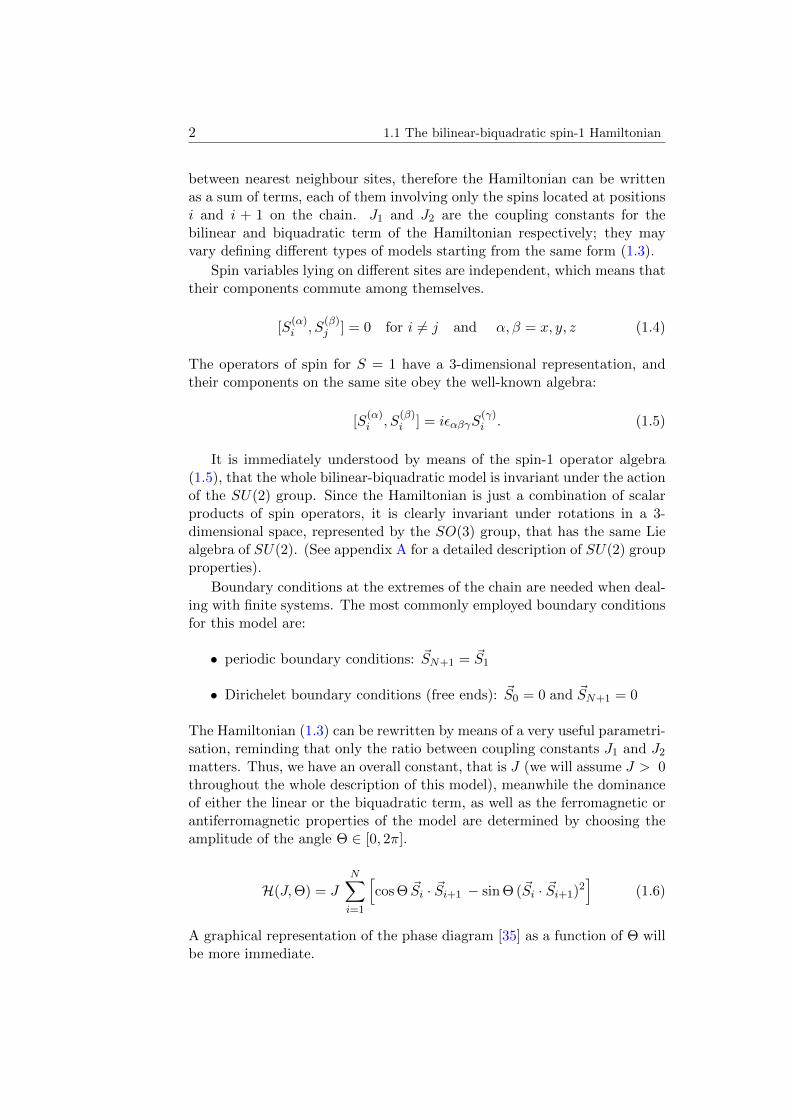
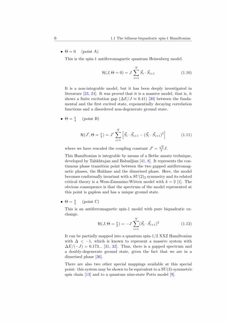
Figure 1.1: Round phase diagram of the bilinear-biquadratic spin-1 model as afunction of the parameter Θ, with tan Θ representing the ratio between the couplingconstants J2 and J1 respectively related to the biquadratic and bilinear terms of theHamiltonian (1.3). It shows four phases: one ferromagnetic and three antiferromag-netic, named trimer, Haldane and dimer phase. The latter two antiferromagneticphases display a gap (∆ > 0) between the ground and the first excited state,whereas the ferromagnetic and trimer phases are gapless (∆ = 0). Points on thediagram labelled by capital letters, single out special models of which we give aquick overview in this chapter. (Picture taken from [7]).
Now we may attempt to describe it. First of all, there are two main re-gions in which we may split it, remembering that Θ measures the dominanceof the two competing terms of the bilinear-biquadratic Hamiltonian. Theregion included between 3
4π and 32π shows a ferromagnetic behavior, while
the remaining region with −π2 < Θ < 3
4π is the antiferromagnetic phase,which has been divided into three further regions:
• −π2 < Θ < −π
4 → trimerised phase
• −π4 < Θ < π
4 → Haldane phase
• π4 < Θ < 3
4π → dimerised phase
In the entire ferromagnetic phase the fully aligned state
|GS〉 = |+ + + + + + + ...〉 ,
is always an eigenstate of the Hamiltonian (1.6), with energy given by
E0 = JN(cos Θ− sin Θ). (1.7)
Using the highest-weight-state basis, we are allowed to evaluate the actionof the whole Hamiltonian (1.6) on an excitation of Stot = N − 1, for which
4 1.1 The bilinear-biquadratic spin-1 Hamiltonian
we simply switch one of the quintet bonds of the ferromagnetic state into atriplet bond. The result gives the following expression for the correspondingeigenvalue of the Hamiltonian [7]:
E(k) = E0 − 2J(cos Θ)(1− cos k) (1.8)
where k is the momentum of the Bethe ansatz wave function of the spinwave excitation, that is an eigenstate of the Hamiltonian defined, using thevalence bond notation, by the following expression:
|k〉 =∑i1 6=i2
eiki1 [i1, i2](i3, i4, ...iN ) (1.9)
where the square brackets indicates a triplet bond connection between thespins located on sites i1 and i2, meanwhile the parentheses indicates spinsall connected by quintet valence bonds.
As we can see, the energy of this excitation is always positive in the range34π < Θ < 3
2π, which means that moving away from the fully aligned statedemands energy, therefore |GS〉 is the system ground state in this phase.
Thus, from the dispersion relation (1.8) we realise that the model remainsgapless in this region of the phase diagram, which means that it shouldbe always possible to create arbitrarily small excitations starting from thesystem ground state |GS〉.
A finite gap opens [19, 20] when, crossing the continuous phase transitionat Θ = 3
4π, the model enters the antiferromagnetic dimerised region, i.e.Θ ∈ [π4 ,
34π]. The main difference distinguishing this phase from the other
gapped phase is the fact that the translational symmetry is broken becausethe system shows a spontaneous tendency to split into pairs of mutuallyinteracting spins. As a consequence the ground state becomes two-fold de-generate. In this range we find the purely biquadratic antiferromagneticHamiltonian (Θ = π
2 ).
An integrable, massless model [41, 8] separates the dimerised phase fromthe Haldane phase, again with a continuous phase transition. The secondgapped phase is a disordered one: the translational symmetry is unbroken,the ground state is unique and there are exponentially decaying correlationfunctions. This range varies from Θ = −π
4 to Θ = π4 and it contains the
antiferromagnetic Heisenberg model (Θ = 0) and the AKLT model (Θ =− arctan 1
3).
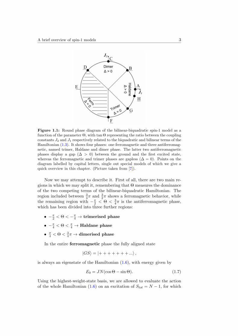
The valence-bond basis provides a simple device to describe the twodifferent types of states belonging to the two different gapped phases, asshown in figure 1.2.
A brief overview of spin-1 models 5
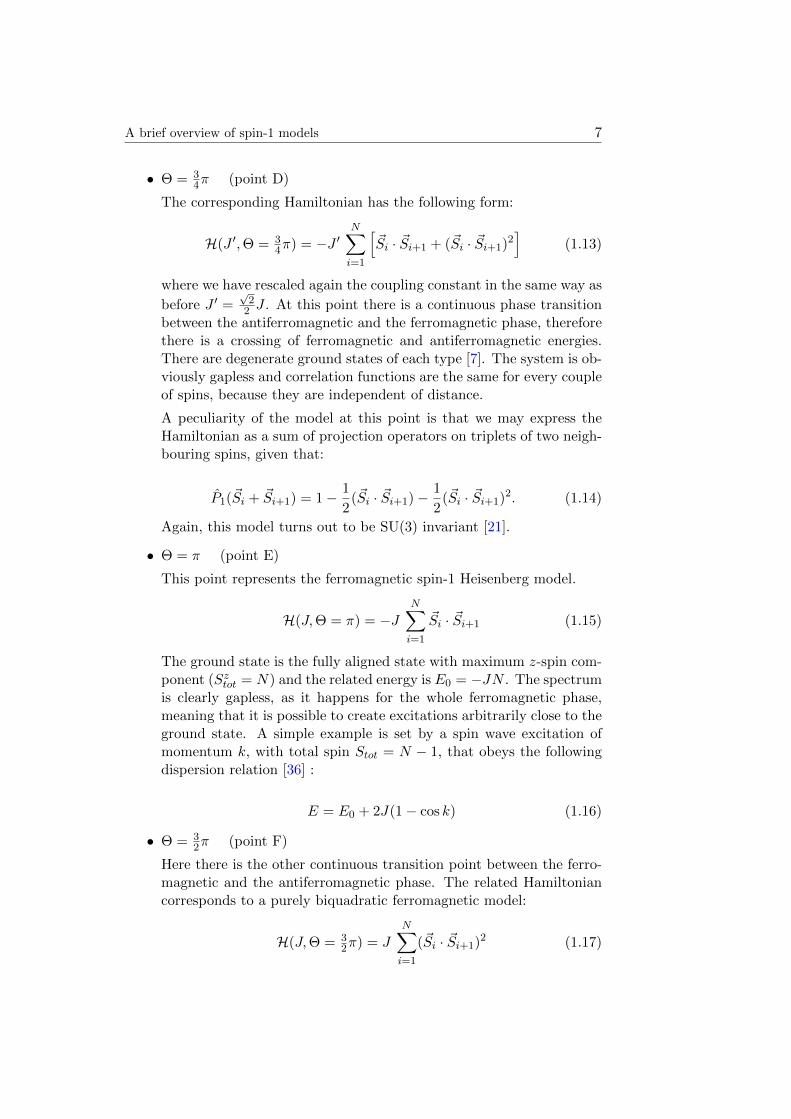
Figure 1.2: Two different states of a spin-1 chain with four sites in the valence-bond pictorial representation. Each site is occupied by two spin-1/2 variables,encircled together by the projector on their triplet state (S = 1). This is a graphicalrepresentation of the constraint that each locus is occupied by one spin-1 variable.Therefore, spin-1/2 variables can form singlet states represented by valence bondsonly with variables located on different sites. The constraint of one particle persite implies one further rule to be obeyed while connecting spins, that is the noncrossing relation, i.e. the valence bonds cannot cross one another an odd numberof times. (Picture taken from [17]).
The first one represents a state with broken symmetry: each pair ofneighbouring spins is connected by two valence bonds. This state is nottranslationally invariant, because we have two allowed configurations re-lated by a shift of one lattice site. The second image represents a state withunbroken symmetry: all spins are connected with one bond to the preced-ing and with another to the following spin. The resulting state is clearlytransaltionally invariant.
Although the last one is the exact VBS ground state for the AKLT model[3, 4], neither of these states is the exact ground state for the bilinear-biquadratic model with arbitrary Θ. However, they may be employed asvariational ground states for those generic models, the first state havinglower energy for Θ > arctan 1
2 and the second one for Θ < arctan 12 [17].
The exact ground state will, however, fit the same symmetry requirementsof these two cases.
Eventually, there is one more antiferromagnetic phase, that is the trime-rised phase in the range −π
2 < Θ < −π4 . Separated from the Haldane
phase by a continuous phase transition corresponding to an integrable criti-cal SU(3)-symmetric model [29, 39], this last phase is expected to be gaplessand spontaneously trimerised, as it is suggested by the symmetry of the val-ues of the soft modes at k = 0,±2
3π [36].Now, let’s try to make a list of all the remarkable points of the phase
diagram and the characteristic features of each phase, starting from Θ = 0.
6 1.1 The bilinear-biquadratic spin-1 Hamiltonian
• Θ = 0 (point A)
This is the spin-1 antiferromagnetic quantum Heisenberg model.
H(J,Θ = 0) = JN∑i=1
~Si · ~Si+1 (1.10)
It is a non-integrable model, but it has been deeply investigated inliterature [23, 24]. It was proved that it is a massive model, that is, itshows a finite excitation gap (∆E/J ≈ 0.41) [30] between the funda-mental and the first excited state, exponentially decaying correlationfunctions and a disordered non-degenerate ground state.
• Θ = π4 (point B)
H(J ′,Θ = π4 ) = J ′
N∑i=1
[~Si · ~Si+1 − (~Si · ~Si+1)
2]
(1.11)
where we have rescaled the coupling constant J ′ =√22 J .
This Hamiltonian is integrable by means of a Bethe ansatz technique,developed by Tahkhtajan and Babudjian [41, 8]. It represents the con-tinuous phase transition point between the two gapped antiferromag-netic phases, the Haldane and the dimerised phase. Here, the modelbecomes conformally invariant with a SU(2)2 symmetry and its relatedcritical theory is a Wess-Zummino-Witten model with k = 2 [1]. Theobvious consequence is that the spectrum of the model represented atthis point is gapless and has a unique ground state.
• Θ = π2 (point C)
This is an antiferromagnetic spin-1 model with pure biquadratic ex-change.
H(J,Θ = π2 ) = −J
N∑i=1
(~Si · ~Si+1)2 (1.12)
It can be partially mapped into a quantum spin-1/2 XXZ Hamiltonianwith ∆ < −1, which is known to represent a massive system with∆E/(−J) = 0.173... [31, 32]. Thus, there is a gapped spectrum anda doubly-degenerate ground state, given the fact that we are in adimerised phase [36].
There are also two other special mappings available at this specialpoint: this system may be shown to be equivalent to a SU(3)-symmetricspin chain [13] and to a quantum nine-state Potts model [9].
A brief overview of spin-1 models 7
• Θ = 34π (point D)
The corresponding Hamiltonian has the following form:
H(J ′,Θ = 34π) = −J ′
N∑i=1
[~Si · ~Si+1 + (~Si · ~Si+1)
2]
(1.13)
where we have rescaled again the coupling constant in the same way as
before J ′ =√22 J . At this point there is a continuous phase transition
between the antiferromagnetic and the ferromagnetic phase, thereforethere is a crossing of ferromagnetic and antiferromagnetic energies.There are degenerate ground states of each type [7]. The system is ob-viously gapless and correlation functions are the same for every coupleof spins, because they are independent of distance.
A peculiarity of the model at this point is that we may express theHamiltonian as a sum of projection operators on triplets of two neigh-bouring spins, given that:
P1(~Si + ~Si+1) = 1− 1
2(~Si · ~Si+1)−
1
2(~Si · ~Si+1)
2. (1.14)
Again, this model turns out to be SU(3) invariant [21].
• Θ = π (point E)
This point represents the ferromagnetic spin-1 Heisenberg model.
H(J,Θ = π) = −JN∑i=1
~Si · ~Si+1 (1.15)
The ground state is the fully aligned state with maximum z-spin com-ponent (Sztot = N) and the related energy is E0 = −JN . The spectrumis clearly gapless, as it happens for the whole ferromagnetic phase,meaning that it is possible to create excitations arbitrarily close to theground state. A simple example is set by a spin wave excitation ofmomentum k, with total spin Stot = N − 1, that obeys the followingdispersion relation [36] :
E = E0 + 2J(1− cos k) (1.16)
• Θ = 32π (point F)
Here there is the other continuous transition point between the ferro-magnetic and the antiferromagnetic phase. The related Hamiltoniancorresponds to a purely biquadratic ferromagnetic model:
H(J,Θ = 32π) = J
N∑i=1
(~Si · ~Si+1)2 (1.17)
8 1.1 The bilinear-biquadratic spin-1 Hamiltonian
Just like the corresponding antiferromagnetic model it is endowed witha SU(3) symmetry and it has massive spectrum with the same disper-sion relation (provided −J → J):
E = E0 + J(3 + 2 cos k) where E0 = JN (1.18)
At point F there is again the possibility of expressing the Hamiltonianas a sum of projection operators [7] of pairs of neighbouring spins ona common singlet state, knowing that:
P0(~Si + ~Si+1) = −1
3+
1
3(~Si · ~Si+1)
2 (1.19)
• Θ = −π4 (point G)
This point corresponds to a continuous phase transition which sepa-rates a gapless antiferromagnetic phase (trimer) from a gapped one(Haldane). Again, we find an exactly integrable model
H(J ′,Θ = −π4 ) = J ′
N∑i=1
[~Si · ~Si+1 + (~Si · ~Si+1)
2], (1.20)
which is usually referred to as Lai-Sutherland Hamiltonian. It is solv-able with the Bethe ansatz [29, 39]. The resulting spectrum is gaplessand the ground state is unique. As its diametrically opposite point(D), this Hamiltonian can be written as a sum of permutation oper-ators and it has a mapping onto a SU(3)-symmetric spin chain. As aconsequence of being a massless model, its critical behaviour shouldbe related to a SU(3)-symmetric conformal theory with k = 1.
• Θ = − arctan(1/3) (point H)
H(J ′′,Θ = − arctan(1/3)) = J ′′N∑i=1
[~Si · ~Si+1 +
1
3(~Si · ~Si+1)
2
](1.21)
where a rescaling of the coupling constant has been performed accord-ing to J ′′ = 3√
10.
This particular model, named AKLT model (after Affleck, Kennedy,Lieb and Tasaki), has known solutions thanks to the valence-bond-solidbasis, which can be used to express the exact form of the ground state,that is unique in the thermodynamic limit. It represents a massivemodel, thus its spectrum has a finite gap and the spin correlations arepurely exponential [3, 4].
A brief overview of spin-1 models 9
One last interesting property of this Hamiltonian is that it may beexpressed as a sum of projection operators onto a quintet state ofspins lying on neighbouring sites. In fact,
P2(~Si + ~Si+1) =1
3+
1
2(~Si · ~Si+1) +
1
6(~Si · ~Si+1)
2 (1.22)

Chapter 2
SU(2) symmetry andcorrespondence with theXXZ model
It was proved that there are some special values of Θ, such as Θ = ±π4 ,±π
2 ,for which the model (1.6) is solvable by means of the Bethe ansatz [31, 41,8, 29, 39].
This technique, which was created in order to find explicitly eigenvaluesand eigenstates of the spin-1/2 Heisenberg chain, is mainly founded on thedefinition of a primary state, that is usually one of the two fully alignedstates, for example we choose the one with the maximum value of the Sztot,on which we act a certain number of times with the ladder operators S−i toget other states with lower values of Sztot. The classification of states arisingin this framework is based on SU(2) quantum numbers, i.e. ~S2
tot and Sztot.
Since the Hamiltonian (1.6) commutes with the z-component of the totalspin, we may choose a basis of eigenstates of Sztot on which we decompose theHamiltonian eigenstates. This kind of approach is allowed just for an SU(2)-invariant system because the commutation properties of the Hamiltonianwith the group generators leads to a decomposition of the total Hilbert spaceof eigenstates into sectors with fixed values of Sztot. Thus, the Hamiltonianappears in a block diagonal form and eigenstates of the same Sztot transformamong themselves under the action of the this matrix operator.
Following this decomposition method, well-known for the spin-1/2 chain,we may be able to apply the Bethe ansatz technique in order to solve thebilinear-biquadratic model in some special cases; among them lies the purebiquadratic model.
Let’s focus our attention, for the moment, on the resulting Hamiltonian(1.6) for Θ = π
2 :
11
12
H(J,Θ = π2 ) = −J
N∑i=1
(~Si · ~Si+1)2 (2.1)
which represents a biquadratic antiferromagnetic model, that is a spin-1chain with a pure biquadratic exchange interaction.
Employing the technique outlined before, paying attention to some nec-essary changes due to the different spin representation, we can find a patternto describe all eigenstates of this Hamiltonian. The spin variables fixed oneach site of the one dimensional lattice can now take three different values ofSzi , and we can represent them through a symbolic notation: |+〉 , |0〉 , |−〉.
Starting with the fully aligned state:
|GS〉 = |+ + + + + + + ...〉 ,
we can build up all other Sztot eigenstates by operating an arbitrary numberof times on this state with a combination of the ladder operators S−i . Weget, then, the classification of states according to their values of Sztot, whichcorrespond to a precise number of deviations from the fundamental state.
Asking that a linear combination of states belonging to the same eigen-value of Sztot forms an eigenstate of the global Hamiltonian, one eventuallygets some constraints on the wavevector k, connected to the wave functiondefined in the Bethe ansatz solution. The general behavior of the pure-biquadratic model eigenstates, which will be fully developed in the followingsections, can be summarised as follows:
• states with a single deviation:these states have the same energy as the fully aligned state. The actionof the pure biqudratic term on these state is null, which means thatthese states do not propagate.
• states with an arbitrary number of isolated deviations:states with isolated deviations are states for which the applicationsof the ladder operators S−i occur neither on the same nor on adja-cent sites. There are up to N/2 possible isolated deviations on aN -spin chain. All of these states are obviously degenerate with thefully aligned state.
• states with two non-isolated deviations:these states contain a couple of the type |+−〉 , |0 0〉 or |−+〉. Accord-ing to the expression of the biquadratic Hamiltonian, these are theonly couples of nearest-neighbour states propagating, therefore theyform a two-string, with energy expressed by:
∆E2 = −J (3 + 2 cos k) (2.2)
SU(2) symmetry and correspondence with the XXZ model 13
where
k =2πl
Nl = 0, 1, 2...N − 1 (2.3)
• states with three non-isolated deviations:these states are inevitably made up of one propagating two-string andan isolated deviation. They have, thus, the same energy expression thetwo-deviation states have, but with some modifications given by thefact that when a two-string propagates through the isolated deviation,it shifts its position on the lattice by two lattice sites.
∆E3 = −J (3 + 2 cos θ) (2.4)
where
θ =2πr ± 2k
N − 2l = 0, 1, 2...N − 3 (2.5)
• states with four non-isolated deviations:these may be interpreted as states with a pair of two-string, whichinteract among themselves while propagating on the chain. It occursthat in special cases the two two-string can unite forming a boundstate and the energy expression of the whole state is given by:
∆E4 = −J [(3 + 2 cos k1) + (3 + 2 cos k2)] (2.6)
whereNk1 = 2πl1 + ϕ l1 = 0, 1, ...N − 1 (2.7)
Nk2 = 2πl2 − ϕ l2 = 0, 1, ...N − 1 (2.8)
cotϕ/2 =−3 sin 1
2(k1 − k2)2 cos 1
2(k1 + k2) + 3 cos 12(k1 − k2)
(2.9)
• states with a higher number of non-isolated deviation:they are basically made up of the former building blocks. Isolateddeviations, which do not propagate, on the one hand and propagatingtwo-strings on the other, which may be forming new structures, suchas two-string bound states.
2.1 Correspondence between XXZmodel and pure-biquadratic model
The rather characteristic features of the formerly described structure ofeigenstates of the biquadratic Hamiltonian can be immediately related to
14 2.1 Correspondence between XXZ model and pure-biquadratic model
the typical one of the XXZ model. The former is a one-dimensional latticemodel described by the Hamiltonian:
H(Jxxz,∆) = −JxxzN∑i=1
[Sxi S
xi+1 + Syi S
yi+1 + ∆Szi S
zi+1
](2.10)
The undeniable similarities between the two families of eigenstates be-come clear once the identifications
∆ = −3
2Jxxz = 2J. (2.11)
are made. Assuming these special values of the parameters, the solutions ofthe spin 1/2 XXZ model, which is known to be integrable via Bethe ansatztechniques [40], resemble exactly the eigenstates of the biquadratic spin-1model under examination. It is well known [40] that the XXZ model for∆ < −1 is massive, i.e. it has a gap, so this mapping is in agreement withthe prediction that the biquadratic spin-1 model lies into the parameterregion π
4 < Θ < 34π, where the bilinear-biquadratic model is supposed to
have a finite gap.
An other interesting consequence of this mapping is the interpretation asspin waves of the deviations, which form essentially a localised structure,named two-string, propagating itself jointly along the spin chain. This hasa strong analogy with what happens in spin-1/2 magnetic systems, wherea single spin flip creates a magnonic excitation. There, magnons interactamong themselves forming bound states; the same happens here for stateswith four or more deviations, in which a couple of two-strings may appear,with the corresponding momenta obeying exactly the same dispersion rela-tion of the XXZ model (2.6).
This correspondence between the eigenstates of these two models waspointed out at first by Parkinson [31], who used the Bethe ansatz to com-pute the energies of the previously listed states, classified by the numberof deviations, that is directly related to the value of the z-component ofthe total spin. This discovered correspondence between XXZ eigenstateswith M deviations and biquadratic Hamiltonian eigenstates with M two-strings supposedly allows us to find the eigenstates and eigenvalues of thebiquadratic model by means of the Bethe ansatz.
Even though the pure-biquadratic has not yet been proved to be an inte-grable model, the mapping proposed by Parkinson leads to a vast knowledgeof the model (2.1), but with some significant reservations.
Following the work outlined by Parkinson [32] we will stay within theframework of periodic boundary conditions comparing the results with theXXZ-model Bethe ansatz equations, which are strictly related to the differ-ent type of boundary conditions imposed on the model (cfr. eq. (2.22)).
SU(2) symmetry and correspondence with the XXZ model 15
Thus, in order to allow the comparison we will restrict ourselves to chainswith an even number of sites and periodic boundary conditions.
Secondly, the mapping on XXZ model is working as long as the stateswith an even number of deviations are concerned. States with an oddnumber of deviations have no representation in the XXZ model; thereforethe suggested mapping is only partial. This can be easily understood by thedimensional analysis of the problem. The XXZ Hamiltonian is a spin-1/2model, therefore each spin variable can take on just two values, whereasthe pure-biquadratic Hamiltonian is a spin-1 model, which means that eachvariable can take on three different values. With N defining the lengthof the chain, the XXZ Hamiltonian operator is 2N × 2N dimensional: thenumber of its eigenstates, amounting to 2N , is definitely lesser than the onegiven by the biquadratic spin-1 Hamiltonian, which belongs to a 3N × 3N
dimensional Hilbert space. Being the latter eigenstates in a larger number,we realise that not every biquadratic eigenstate can be mapped into theXXZ chain, but only those ones with peculiar features that will be definedlater on. We stress the fact that we can map each XXZ eigenstate into abiquadratic model eigenstate, but the converse is not true, because of thedimensional discrepancy.
There is one further complication: thanks to numerical simulations onfinite length chains [32] it was possible to check out computationally thatthe energy levels do, in fact, match for each even number of deviations,apart from M = N/2. The mapping into the XXZ model is not working forstates with Sztot = 0, which is a big disappointment, since this is certainlythe largest sector of eigenstates of the Hamiltonian and the most importantone because it contains the ground state for the antiferromagnetic model.
The reason why this mapping is not complete is not clear yet, but itshould be crucial to understand it. We could make some assumptions basedon the fact that the number of couples |+−〉 would then fill entirely theavailable sites, preventing thus to the two-strings to propagate freely alongthe chain. This argument is not really convincing, because if this unre-solved matter has to be ascribed to the progressively reducing ”availableroom for propagation” on the chain, there would have been some kind of de-viation from the XXZ correspondence pattern as the number of two-stringsapproached N/2. This question remains still unsolved.
2.2 The XXZ model: Bethe ansatz
The XXZ model is a spin-1/2 quantum model defined on a one dimensionallattice of length N . It is essentially a chain of N sites with a spin variableon each locus. Differently from the simpler Heisenberg model, that is com-pletely isotropic -the coupling constants along all three cartesian axes areequal-, the XXZ model introduces an isotropy along the z-axis, which may
16 2.2 The XXZ model: Bethe ansatz
be quantified by the parameter ∆. The XXZ Hamiltonian is:
H (Jxxz,∆) = −JxxzN∑i=1
[Sxi S
xi+1 + Syi S
yi+1 + ∆Szi S
zi+1
](2.12)
The anisotropic coupling along the z-axis, achieved by means of a pa-rameter ∆ 6= 1, breaks the SU(2) invariance of this spin model. Therefore,the XXZ Hamiltonian does not commute with the x and y components ofthe total spin Sxtot and Sytot anymore, but it still commutes with Sztot, whichmeans that the eigenvalues of Sztot are still good quantum numbers for thismodel. Thanks to this crucial property of the XXZ Hamiltonian we areallowed to decompose the Hilbert space of its eigenstates into sectors withfixed Sztot
H =∞⊕n=0
H(n) (2.13)
and proceed with the usual Bethe ansatz technique, that is founded on theassumption that a general eigenstate of the Hamiltonian may be found bysetting an ansatz on the wave function form. The amount of work willbe reduced if we could be able to find operators that commute with theHamiltonian, allowing us to restrict the Hilbert space of states, in orderto work within sufficiently narrow subspaces, which will be later extendedemploying the symmetries of the system, only once the solutions are found.
This is the reason why we proceed assuming that a given value of devi-ations, represented by M , from the fully aligned state
|0〉 = |↑↑↑↑↑↑↑↑ ...〉 ,
is uniquely characterising the subspace in which we work. We immediatelyrealise that Sztot = n = N/2−M . Thus fixing M is a simple way of choosinga sector of the block diagonal XXZ Hamiltonian, for which Sztot is fixed.Whereas the fully aligned states (M = 0,M = N) are the two ground statesof a ferromagnetic system, the fundamental state of the antiferromagneticmodel would be located in the Sztot = 0, that means of course M = N/2.
A generic eigenstate belonging to a fixed-M sector can be written as alinear combination of all the states with different locations of the M downspins on the chain sites, labelled by the integers ni, i = 1, 2...M .
|Ψ〉 =∑n
f(n1, n2, ..., nM )S−n1S−n2
... S−nM |0〉 (2.14)
The sum runs over all the M ! permutations of the M position indices, thatare supposed to be ordered 0 ≤ i1 < i2 < ... < iM ≤ N . The coefficients
SU(2) symmetry and correspondence with the XXZ model 17
of this combination are functions of indices and their global form can bedetermined by imposing that |Ψ〉 is an eigenstate of the Hamiltonian.
H(Jxxz,∆)|Ψ〉 = E|Ψ〉 (2.15)
It is convenient to use the XXZ-model Hamiltonian formulation writtenin terms of ladder operators:
H(Jxxz,∆) = −12J
xxzN∑i=1
[S+i S−i+1 + S−i S
+i+1 + 2∆ Szi S
zi+1
](2.16)
The action of the former Hamiltonian operator on a state given by (2.14),gives the following eigenvalue equation:
− 12J∑i
(1− δni,ni+1
)[f(n1, ...ni + 1, ni+1, ..., nM )+
+ f(n1, ..., ni, ni+1 − 1, ..., nM )]+
+ J∆[−1
4N +M −∑i
δni+1,ni+1
]f(n1, ...ni, ni+1, ..., nM ) =
= Ef(n1, ...ni, ni+1, ..., nM )
(2.17)
Let us formulate now the basic ansatz regarding the wave function form:
f(n1, ......, nM ) =∑P
A(P )e i∑Mi=1 kP (i)ni (2.18)
where the sum runs over the M ! permutations P of the M site indices. k arenamed quasi-momenta, because the former expression formally resembles asuperposition of plane waves with momenta kP (i) with i = 1, ..,M .
Starting from the eigenstate equation (2.17) for the case ni+1 6= ni+1 ∀ i =1, ...,M , we can ignore the presence of the δni+1,ni+1 terms, and using theansatz on the wave function, we find the expression of the energy of ageneral eigenstate as a function of the quasi momenta:
E = E0 +
M∑i=1
[Jxxz(∆− cos kj)
](2.19)
in which we have defined the energy of the fully aligned state |0〉 = |↑↑↑↑↑↑↑↑ ...〉as E0 = −1
4NJxxz.
In order to find the whole expression of the wave functions we needto calculate the coefficients A(P ), which do not enter explicitly in the for-mer determination of the energy dispersion relation. They are fixed by theanalysis of the occurrence of deviations on two neighbouring sites, that isni + 1 = ni+1 for just one value of i. Taking into account the δni+1,ni+1 ,

18 2.2 The XXZ model: Bethe ansatz
equation (2.17) can be rewritten as a series of constraints for the wave func-tion:
f(n1, ...ni + 1, ni + 1, ..., nM ) + f(n1, ...ni, ni, ..., nM ) =
= 2∆ f(n1, ...ni, ni+1, ..., nM )(2.20)
for i = 1, ..M , which can be easily satisfied choosing the following expressionfor the amplitude coefficients:
A(P ) = ε(P )∏l<j
(ei(kP (l)+kP (j)) − 2∆eikP (l) + 1
)(2.21)
with ε(P ) being the sign of the permutation P .The quasi momenta are not determined directly by means of the appli-
cation of the Bethe ansatz technique to the Hamiltonian of the XXZ model,but they may be found employing different conditions, which they must sat-isfy. This last set of equations is determined by the assumption of a certaintype of boundary conditions on the system, which univocally fix the valuesof the quasi-momenta.
Assuming periodic boundary conditions, i.e. ~SN+1 = ~S1, the XXZ sys-tem is known to be an exactly integrable model.
The imposition of periodic boundary conditions on the wave functionresults in a set of equations:
eikjN = (−1)M−1∏l 6=j
ei(kj+kl) + 1− 2∆eikj
ei(kj+kl) + 1− 2∆eiklj = 1, 2...M (2.22)
which leads to:
kjN = −M∑l=1
Θ(kj , kl) + 2πIj (2.23)
where we have defined:
Θ(kj , kl) = 2 tan−1∆ sin 1
2(kj − kl)cos 1
2(kj + kl)−∆ cos 12(kj − kl)
(2.24)
with
Ij =M + 1− 2j
2, j = 1, 2, ...M. (2.25)
Tuning the parameters which the XXZ model Hamiltonian depends on,we may be able to get the same energy spectrum of the biquadratic Hamil-tonian (restricted to states with an even number of deviations). Therefore,we set
∆ = −3
2Jxxz = 2J.
This identification used in equations (2.19) and (2.24) with M = 1 andM = 2 leads directly to the expressions for E2 and E4 for states of thebiquadratic Hamiltonian with two and four deviations, respectively (2.2)(2.6).
SU(2) symmetry and correspondence with the XXZ model 19
2.3 The purely biquadratic Hamiltonian: Betheansatz
Let’s focus our attention now on the biquadratic term of the Hamiltonian(1.6), which reads:
H(J,Θ =π
2) = −J
N∑i=1
(~Si · ~Si+1)2 (2.26)
We can write it down in a slightly different form, which will turn out to bemore practical for our purposes. Defining the operator hi = (~Si · ~Si+1)
2− 1,we may write
H(J,Θ =π
2) = −J
N∑i=1
hi + E0 (2.27)
where
E0 = −NJ (2.28)
is the energy associated with the fully aligned state (a state in which theeigenvalue is Szi = 1 for each spin variable):
|GS〉 = |+ + + + + + + + + ...〉 .
The full Hamiltonian is therefore a combination of spatially localisedoperators, that is, operators which act only on pairs of neighbouring sites.Writing down a basis for a couple of spins, ordered according to the followingscheme:
|++〉 |+0〉 |0+〉 |+−〉 |00〉 |−+〉 |0−〉 |−0〉 |−−〉 (2.29)
we can use it to evaluate the product ~Si · ~Si+1 and eventually put hi into amatrix form:
~Si · ~Si+1 =
10 11 0
−1 1 01 0 10 1 −1
0 11 0
1
(2.30)
20 2.3 The purely biquadratic Hamiltonian: Bethe ansatz
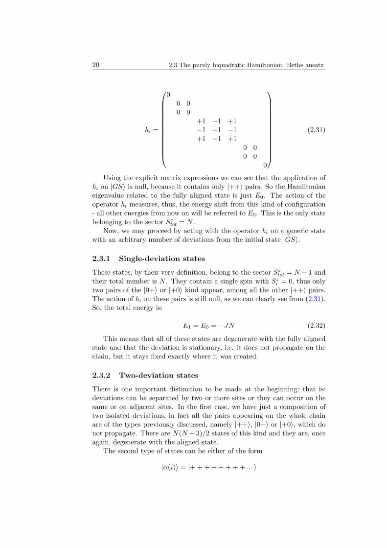
hi =
00 00 0
+1 −1 +1−1 +1 −1+1 −1 +1
0 00 0
0
(2.31)
Using the explicit matrix expressions we can see that the application ofhi on |GS〉 is null, because it contains only |++〉 pairs. So the Hamiltonianeigenvalue related to the fully aligned state is just E0. The action of theoperator hi measures, thus, the energy shift from this kind of configuration- all other energies from now on will be referred to E0. This is the only statebelonging to the sector Sztot = N .
Now, we may proceed by acting with the operator hi on a generic statewith an arbitrary number of deviations from the initial state |GS〉.
2.3.1 Single-deviation states
These states, by their very definition, belong to the sector Sztot = N − 1 andtheir total number is N . They contain a single spin with Szi = 0, thus onlytwo pairs of the |0+〉 or |+0〉 kind appear, among all the other |++〉 pairs.The action of hi on these pairs is still null, as we can clearly see from (2.31).So, the total energy is:
E1 = E0 = −JN (2.32)
This means that all of these states are degenerate with the fully alignedstate and that the deviation is stationary, i.e. it does not propagate on thechain, but it stays fixed exactly where it was created.
2.3.2 Two-deviation states
There is one important distinction to be made at the beginning; that is:deviations can be separated by two or more sites or they can occur on thesame or on adjacent sites. In the first case, we have just a composition oftwo isolated deviations, in fact all the pairs appearing on the whole chainare of the types previously discussed, namely |++〉, |0+〉 or |+0〉, which donot propagate. There are N(N − 3)/2 states of this kind and they are, onceagain, degenerate with the aligned state.
The second type of states can be either of the form
|α(i)〉 = |+ + + +−+ + + ... 〉
SU(2) symmetry and correspondence with the XXZ model 21
or|β(i)〉 = |+ + + + 0 0 + + + ... 〉 ,
where the first deviation is located at the site i in both cases.Clearly, there are 2N states of this kind. A general eigenstate will be a
linear combination of |α(i)〉 and |β(i)〉:
|Ψ〉 =∑i
(ai |α(i)〉+ bi |β(i)〉) (2.33)
with coefficients ai and bi determined by the constraint that this is an eigen-state of the biquadratic Hamiltonian:
H(J,Θ = π2 ) |Ψ〉 = E2 |Ψ〉 (2.34)
which has to satisfy the periodic boundary conditions, too.A solution of this equation is given by ai = Aeiki, if the wavevector k
satisfies the relation:
∆E = E2 − E0 = −J(3 + 2 cos k). (2.35)
These states are not degenerate with the aligned state anymore. This isa consequence of the fact that these states contain pairs, like |−+〉, |+−〉 or|0 0〉, which transform among themselves under the action of the operatorhi , producing a shift of the position of the deviation, too. The result isa propagating wave, which is very similar in its dispersion relation to spinwaves of magnetic models. As we stated, this is exactly the case for theXXZ model.
2.3.3 Three-deviation states
Again we must distinguish between isolated deviations and non isolated de-viations. The former considerations still apply for the isolated-deviationstates. Let’s focus now on states with three deviations occurring on neigh-bouring sites or (two of them at most) on the same site. We find states ofthese types:
|α(i, j)〉 = |+ + 0i
+ + 0j
0 + + + ... 〉
|β(i, j)〉 = |+ + 0i
+ +−j
+ + +... 〉,
|γ(i, j)〉 = |+ 0 0i
+ + 0j
+ + + ... 〉
|δ(i, j)〉 = |+ + −i
+ + 0j
0 + +... 〉
which we can linearly combine with coefficients aij , bij , cij and dij respec-tively. Imposition of periodic boundary conditions yields relations amongthem:
aij = cj+1,i+N
22 2.3 The purely biquadratic Hamiltonian: Bethe ansatz
cij = aj,i+N−1
bij = dj,i+N
dij = bj,i+N
Only two of these weight coefficients are independent, because the setof states |α(i, j)〉 and |γ(i, j)〉 are essentially the same, modulo periodicboundary conditions. The same happens for |β(i, j)〉 and |δ(i, j)〉.
As usual we get our set of constraints on the coefficients by imposingthat a linear combination |Ψ〉 of these four types of states is an eigenstate ofthe biquadratic Hamiltonian. We eventually get to solve a set of equationsfor a single parameter aij .
A further simplification comes from the requirement of the translationalinvariance, that means:
aij = eikian where n = j − i (2.36)
By means of this procedure we are allowed to find a solution of the Betheansatz type:
an = A1eiθn +A2e
−iθn (2.37)
provided θ satisfies:
∆E
−J − 3 = eiθ + e−iθ, (2.38)
which is the dispersion relation for a three-deviation state:
E3 = E0 − J (3 + 2 cos θ) (2.39)
Furthermore, the constraint on |Ψ〉 to be an Hamiltonian eigenstatetranslates into an equation which fixes the value of θ:
eiθ(N−2) = e−2ik ⇐⇒ θ =2πr ± 2k
N − 2r = 0, 1, 2...N − 3 (2.40)
Since k is defined as k = 2πlN , with integer l, it may happen that r
and l combine in giving a multiple of N − 2, that means θ = 2πpN , with
integer p, which reproduces the result previously discussed for two-deviationstates. Thus, apart from this kind of states, obviously degenerate withtwo-deviation states, eigenstates of the biquadratic Hamiltonian with threedeviations correspond to a propagating couple interacting with a stationarydeviation. When the two-string has to pass through the single deviation, itcauses its shift by two site positions; this is pointed out by the presence ofthe N − 2 factor. These states belong to the Sztot = N − 3 sector, but some
SU(2) symmetry and correspondence with the XXZ model 23
of them belong to Stot = N − 2 and the rest of them to Stot = N − 3. Thetotal number of them amounts to 2N(N − 2).
Since θ is defined by equation (2.38), θ is always real, which means thatthere are not three-deviation bound states. This is an important resultbecause it states that an odd number of deviations cannot combine to forma system bound state.
2.3.4 Four-deviation states
Once again, we have to discard at first states with isolated deviations, andthen we may apply the same Bethe ansatz technique outlined in the previouscases. Computational complications arise since the more deviations we takeunder consideration, the wider the variety of states is. Nevertheless, it isstill possible to find an analytical solution of the case Sz = N − 4. Wecan incorporate right from the beginning the periodic boundary conditionsrestricting the possible cases of four deviations to the following ones:
|α(i, j)〉 = |+ + 0i0 + + 0
j0 + + + ... 〉
|β(i, j)〉 = |+ +−i
+ + 0j
0 + + + ... 〉
|γ(i, j)〉 = |+ + −i
+ + −j
+ + + ... 〉,
where two two-strings are separated. When the two two-strings interact wehave the following cases:
|α(i, i+ 2)〉 = |+ + 0i0 0 0 + + + + + ... 〉
|β(i, i+ 1)〉 = |+ +−i
0 0 + + + + + ... 〉
|β(i, i+N − 2)〉 = |+ + 0 0 −i
+ + +... 〉
|γ(i, i+ 1)〉 = |+ + −i−+ + + + + ... 〉
|ρ(i)〉 = |+ + 0i
+− 0 + + + + + +... 〉
|σ(i)〉 = |+ + 0i−+ 0 + + + + + +... 〉
with the respective weight coefficients ai,j , bi,j , ci,j , ai,i+2, bi,i+1, bi,i+N−2,ci,i+1, ri and si.
The procedure is exactly the same applied for the case N = 2 and N = 3.Imposition of translational invariance and periodic boundary conditions areneeded to find a solution of the eigenstate constraints given by the actionof the Hamiltonian on a linear combination of the previously listed states,which transforms among themselves. Again, the most general Bethe ansatzsolution can be expressed in the form:
24 2.3 The purely biquadratic Hamiltonian: Bethe ansatz
aij = eikian where n = j − i (2.41)
withan = A1e
ik1n +A2eik2n where k1 + k2 = k. (2.42)
Periodic boundary conditions require: A1A2
= eik2N and the vanishingcondition on the determinant of the system of constraints coming from theeigenvalue equations, gives:
ε(ε− 3− 2 cos k1)(ε− 3− 2 cos k1)(ε− 6− 2 cos k1 − 2 cos k2) = 0, (2.43)
where we have defined ε = (E4−E0)−J . These four different values of ε corre-
spond to four different cases:
• ε = 0 → no two-strings. Only isolated deviations make up astate with energy equal to E0, thus degenerate with the fully alignedstate.
• ε = 3+2 cos k1 → one two-string with momentum k1 interactingwith two stationary isolated deviations. The energy of this kind ofstates resembles the one of the two-deviation or three-deviation states,when a two-string is formed. It can be noticed that the dispersionrelation is basically the same as (2.35).
• ε = 3 + 2 cos k2 → one two-string with momentum k2 and twoisolated deviations. Same observations stand.
• ε = 6 + 2 cos k1 + cos k2 → two two-strings, each one withits own momentum k1 or k2. There are two two-strings formed withthe available four deviations. They interact on the chain exactly inthe same way spin waves do on a spin-1/2 chain, since the energy isprecisely the sum of the single energies of the two two-string. Theycan even bond together and form bound states with complex momentak1and k2, provided their sum, representing the total momentum, staysreal.
The last case is also the most interesting one. Some other conditions onthe determinant of the eigenvalue equations concerning special low value ofn, making use of the definitions (2.42) in the case
ε = 6 + 2 cos k1 + 2 cos k2 (2.44)
yields the condition:
eik2N = −ei(k1+k2) + 1 + 3eik2
ei(k1+k2) + 1 + 3eik1(2.45)
SU(2) symmetry and correspondence with the XXZ model 25
Naming eik2N = e−iϕ, and keeping in mind relation (2.42) between k1and k2, we finally get a simple expression of the wavevectors describing astate containing two two-strings:
Nk1 = 2πl1 + ϕ Nk2 = 2πl2 − ϕ l1, l2 ∈ Z (2.46)
where ϕ is defined by
cotϕ/2 =−3 sin 1
2(k1 − k2)2 cos 1
2(k1 + k2) + 3 cos 12(k1 − k2)
(2.47)
The energy of two interacting 2-string is given by (2.44):
E4 = E0 − J [(3 + 2 cos k1) + (3 + 2 cos k2)] . (2.48)
In the thermodynamic limit, the real values of k1 and k2 should form acontinuum of states lying inside a cosine-shaped upper and lower profile,meanwhile the bound states will form a line below or above this diagramaccording to the positive or negative sign of the coupling constant J .
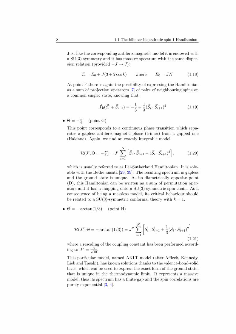
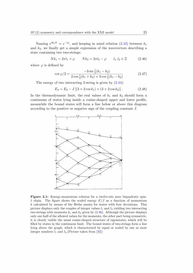
Figure 2.1: Energy-momentum relation for a twelve-site pure biquadratic spin-1 chain. The figure shows the scaled energy E/J as a function of momentumk calculated by means of the Bethe ansatz for states with four deviations. Thispicture displays only the couples of integer values l1 and l2 yielding two interactingtwo-strings with momenta k1 and k2 given by (2.46). Although the picture displaysonly one half of the allowed values for the momenta, the other part being symmetric,it is clearly visible the usual cosine-shaped structure of eigenstates, which will befilled by states in the continuous limit. The bound states of two-strings form a linelying above the graph, which is characterised by equal or scaled by one at mostinteger numbers l1 and l2.(Picture taken from [32])
26 2.4 Note on the correspondence of states
2.4 Note on the correspondence of states
As previously stated, we cannot find a complete correspondence between thebiquadratic Hamiltonian eigenstates and the spin-1/2 XXZ model ones, be-cause the first model has definitely many more states. Just a small amountof them will be mapped into the XXZ states thanks to the equivalence es-tablished in section 2.1, paying attention to the fact that the correspondenceoccurs between spin-1 pairs of the biquadratic modes and single deviationson the XXZ model. We have to bear in mind that the analytical expressionof the Bethe ansatz wave function coefficients which links the two modelsuniquely applies to some special case of spin-1 couples, i.e. only the propa-gating couples
|+−〉 , |00〉 , |−+〉suitably combined to form an Hamiltonian eigenstate, can be mapped intosingle deviations, i.e. a |−〉, on the spin-1/2 chain.
The equivalence lies just in the propagation modes along the chain, whichresemble the spin waves of the XXZ model, because of the localisation prop-erty and the interaction among two-strings in the biquadratic model, whichshows the same rules of spin-waves composition in magnetic systems. How-ever, a large amount of states of the biquadratic Hamiltonian cannot bemapped into the XXZ model because there is not enough room in the Hilbertspace of states. In particular, the non-propagating spin-1 pairs:
|++〉 , |+0〉 , |0+〉 , |0−〉 , |−0〉 , |−−〉
may be thought as having all the same representation on the spin-1/2 chain.In fact, they are all equivalent to the background set, made up of all |↑〉,within which the deviations, represented by |↓〉, run forming the spin waves.
The lack of means to represent the latter set of couples, which are neces-sary in particular to build up the states with an odd number of deviations,but also appear every time an isolated deviation occurs on the chain, ispreventing us from completing the entire mapping between the two models.
Chapter 3
SU(3) symmetry and thebilinear Heisenberg chain
In the introduction about the bilinear-biquadratic Hamiltonian, we havestressed the importance of the symmetry properties related to this partic-ular quantum model. In the previous chapter it was developed an SU(2)-symmetric approach, because the entire model is invariant under that group,regardless of the value of Θ, which selects a point on the phase diagram (Seefig.1.1).
However, it can be shown that the bilinear-biquadratic Hamiltonian (1.6)at some special points is endowed with more symmetry properties, namelyit is invariant under the larger SU(3) group, which contains SU(2) as asubgroup. These special points are located on the phase diagram at:
• Θ = π2 (point C) and Θ = −π
2 (point F). Antiferromagnetic (−J) andferromagnetic (+J) pure-biquadratic spin-1 Hamiltonian, respectively.
HbiQ(±J) = ± JN∑i=1
(~Si · ~Si+1)2 (3.1)
• Θ = 34π (point D) and Θ = −π
4 (point G). Antiferromagnetic-ferromagnetictransition point (−J) and Lai-Sutherland model (+J) respectively.
HLS(±J) = ± JN∑i=1
[~Si · ~Si+1 + (~Si · ~Si+1)
2], (3.2)
3.1 SU(3) Heisenberg chain
Exactly in the same way as it happens for SU(2), we may build up a SU(3)Heisenberg model employing the same Hamiltonian structure with nearest-neighbour interactions, replacing the well-known SU(2) spin operators with
27
28 3.1 SU(3) Heisenberg chain
the SU(3) generators. Bearing in mind that there are eight of them, theresulting Heisenberg Hamiltonian structure is:
HSU(3)(J) = J
N∑i=1
8∑α=1
λαi λαi+1 , (3.3)
where i = 1, 2, ..., N labels the lattice site to which the Gell-Mann matrixλα is referred, whereas α running from 1 to 8 indicates that the sum is takenall over the SU(3) generators. (See the related appendix B for definitionsand conventional notations applied for the SU(3) group).
Since SU(3) has two non equivalent fundamental representations [3] and[3] (for further details, see appendix B), there are basically two possible waysof defining this SU(3) Hamiltonian:
• the first one is built up using the same representation, either funda-mental or antifundamental, on all sites of the chain;
• the second one is build up using alternatively fundamental and anti-fundamental representations respectively on odd and even sites.
These two different models can be related to the two different types ofSU(3)-invariant spin-1 Hamiltonians expressed by (3.1) and (3.2). A simpleway of showing the equivalence between the SU(3) Heisenberg chain andthe spin-1 models [13] is based on the identification of the spin operatorsS1, S2 and S3 with the three Gell-Mann matrices:
λ7i =
0 0 00 0 −i0 i 0
− λ5i =
0 0 i0 0 0−i 0 0
λ2i =
0 −i 0i 0 00 0 0
(3.4)
It is sufficient to have three of the SU(3) generators to reproduce theSU(2) subalgebra. Moreover, it is important to stress that we may havechosen other perfectly fine representations (some examples are described inappendix A) of the spin-1 operators, which fulfill the same algebra, but leadus to a different mapping into the SU(3) generators, maybe involving otherGell-Mann matrices. The chosen mapping, with
S1i = λ7i S2
i = −λ5i S3i = λ2i (3.5)
is particularly convenient to prove the equivalence relation between the twomodels under investigation. The mapping of all other Gell-Mann matricesis performed explicitly by calculating the squares and the mixed products ofthe spin components (for details see appendix C). The final expression for aSU(2)-symmetric model of the form
H(α, β) =
N∑i=1
[α(~Si · ~Si+1) + β(~Si · ~Si+1)
2]
(3.6)
SU(3) symmetry and the bilinear Heisenberg chain 29
as a function of the SU(3) generators is:
H(α, β) =
N∑i=1
α (λ2iλ2i+1 + λ5iλ
5i+1 + λ7iλ
7i+1)+
+N∑i=1
12β (λ8iλ
8i+1 + λ3iλ
3i+1 + 8
3 + λ1iλ1i+1 − λ2iλ2i+1 + λ4iλ
4i+1+
− λ5iλ5i+1 + λ6iλ6i+1 − λ7iλ7i+1)
(3.7)
For α = 0 and β = ±J the Hamiltonian (3.6) reproduces the purebiquadratic (anti-)ferromagnetic model, therefore the same choice of the pa-rameters α and β in equation (3.7) guarantees that the resulting expressionas function of the SU(3) generators is representing exactly the biquadraticHamiltonian:
HbiQ(±J) = H(α = 0, β = ±J) = ±12J
N∑i=1
[ λ8iλ8i+1 + λ3iλ
3i+1+
+ λ1iλ1i+1 − λ2iλ2i+1 + λ4iλ
4i+1 − λ5iλ5i+1 + λ6iλ
6i+1 − λ7iλ7i+1 ]± 4
3JN
(3.8)
Now, let’s define properly the SU(3)-symmetric Heisenberg chain withalternate fundamental and antifundamental representations:
HF⊗A(±J) = ±JN/2∑i=1
8∑α=1
[λα2i−1 λ
α2i + λ
α2i λ
α2i+1
](3.9)
where the antifundamental representations [3] have been placed on evensites, whereas fundamental representations [3] were employed to describeodd sites.
It is clear, from equation (3.8), that the equivalence relation between thespin-1 biquadratic and the SU(3) chain
HbiQ(±J) = −12HF⊗A(±J)± 4
3JN (3.10)
may be performed by means of two very simple modifications, such as anoverall rescaling factor of −1
2 and an additive constant which basically justshifts the energy eigenvalues.
For the sake of completeness, we just hint at the fact that it is alsopossible to find the equivalence relation connecting the Lai-Sutherland modelwith the SU(3) chain using the same type of representation both on evenand odd sites; that is:
HLS(±J) = 12HF⊗F (±J)± 4
3JN (3.11)
30 3.2 SU(3)-symmetry of the pure biquadratic spin-1 model
The equivalence is found by fixing the parameters α = β = ±J in equation(3.7). Thus, the formulation in terms of Gell-Mann matrices becomes:
HF⊗F (±J) = ±JN∑i=1
8∑α=1
λαi λαi+1 (3.12)
3.2 SU(3)-symmetry of the pure biquadratic spin-1 model
Let’s focus now on the antiferromagnetic model with pure biquadratic ex-change:
HbiQ(J) = −JN∑i=1
(~Si · ~Si+1)2 (3.13)
in its SU(2)-symmetric structure.The mapping (3.5) proposed in the previous section is very useful to
the aim of showing the equivalence between the spin-1 purely biquadraticmodel and a Heisenberg Hamiltonian endowed with SU(3) symmetry. How-ever, it turns out to have a complicated interpretation of in terms of SU(2)operators. This framework, in fact, leads to a mapping of quantum num-bers, which is not very effective in order to classify the pure biqadraticmodel eigenstates, that spontaneously organise themselves according to theSU(2)-symmetric structure outlined in section 2.3.
The formerly discussed mapping leads to the following relations betweenSU(3) and SU(2) operators:
T 32i+1 = 1
2 λ32i+1 = 1
2
[(S2
2i+1)2 − (S1
2i+1)2]
(3.14)
Y2i+1 = 1√3λ82i+1 = (S3
2i+1)2 − 2
3 (3.15)
These identities work only for odd sites, on which we deliberately choseto have a fundamental representation of the SU(3) group, whereas, foreven sites, operators belonging to the antifundamental representation areinvolved, which lead to an extra minus sign due to the fact that both λ3 andλ8 are real matrices (cfr. appendix B):
T32i = 1
2 λ32i = −1
2λ32i (3.16)
Y 2i = 1√3λ82i = − 1√
3λ82i (3.17)
The consequence of using alternate representations on global quantum num-bers of the entire SU(3) chain can be actually incorporated in an alternateminus sign for odd and even sites:
T 3tot = 1
2
N∑i=1
(−1)i+1λ3i =N∑i=1
(−1)i+1 12
[(S2i )2 − (S1
i )2]
(3.18)
SU(3) symmetry and the bilinear Heisenberg chain 31
Ytot = 1√3
N∑i=1
(−1)i+1λ8i =N∑i=1
(−1)i+1[(S3i )2 − 2
3
](3.19)
Although this mapping between SU(3) and SU(2) quantum numbers isquite easy to find, there is the main disadvantage of having a non diagonalform of S3,
S3 =
(0 −i 0i 0 00 0 0
)(3.20)
that makes the interpretation in terms of Sz eigenstates very intricate, be-cause of the eigenstates form (A.9).
The matter is, then, finding a representation of the spin algebra thathas one of the three spin components, usually Sz in a diagonal form. Themost convenient choice is done organising the Sz eigenvalues 0,±1 on thediagonal in a slightly different order from usual:
Sz =
1 0 00 −1 00 0 0
(3.21)
leading to the set of eigenvalue (A.11). The remaining consistent choicefor the matrices representing the Sx and Sy spin operators are defined in(A.10) in appendix A. Now the obvious advantage of selecting this particularform of the spin components is that the Sz operator coincide with the thirdGell-Mann matrix λ3.
3.3 Mapping of the biquadratic Hamiltonian intoa SU(3) spin chain
Once established the fundamental relation Sz = λ3, we can write downthe complete mapping between the spin-1 operators of the pure-biquadraticHamiltonian and the Gell-Mann matrices of the SU(3) Heisenberg chain:
Sx =1√2
(λ4 + λ6) Sy =1√2
(λ5 − λ7) (3.22)
(Sx)2 =1
2(λ1 − 1√
3λ8 +
4
3) (Sy)2 =
1
2(−λ1 − 1√
3λ8 +
4
3) (3.23)
(Sz)2 =1
3(√
3λ8 + 2) (3.24)
SxSy =1
2(λ2 + iλ3) SySx =
1
2(λ2 − iλ3) (3.25)
32 3.3 Mapping of the biquadratic Hamiltonian into a SU(3) spin chain
SySz =1
2√
2( iλ4 + λ5 + iλ6 + λ7) SzSy =
1
2√
2( −iλ4 + λ5 − iλ6 + λ7)
(3.26)
SxSz =1
2√
2( λ4 − iλ5 − λ6 + iλ7) SzSx =
1
2√
2( −λ4 + iλ5 − λ6 − iλ7)
(3.27)Let’s proceed with the mappping of the pure-biquadratic model (3.13)
into a SU(3) symmetric model. The computational effort would be a lit-tle more using this mapping than the previously discussed one (3.5), but itmakes very immediate the mapping of the biquadratic Hamiltonian eigen-states with SU(3) quantum numbers T 3 and Y .
In order to simplify at minimum the algebra, we need to invert the log-ical process and using the inverse map, expressing the SU(3) operators ascombinations of the three spin components, their squares and mixed prod-ucts. The reason behind this choice lies in the fact that we will obtain anexpression containing SU(2) operators, which will be considerably easier tomanipulate in order to recover the pure-biquadratic Hamiltonian form. Thisis due to the much simpler Lie algebra of SU(2), built upon three commuta-tion rules (A.2) and one basic relation among the spin squares (A.13). Fromthe structure constant table B.1, we see that the SU(3) algebra would becertainly more difficult to deal with.
Inverting the former relations, we obtain the conventional map for thefundamental representation generators:
λ1i = (Sxi )2 − (Sxi )2 (3.28)
λ2i = Sxi Syi + Syi S
xi (3.29)
λ3i = Sz = −i(Sxi Syi − S
yi S
xi ) (3.30)
λ4i = 1√2(Sxi + Sxi S
zi + Szi S
xi ) (3.31)
λ5i = 1√2(Syi + Syi S
zi + Szi S
yi ) (3.32)
λ6i = 1√2(Sxi − Sxi Szi − Szi Sxi ) (3.33)
λ7i = 1√2(−Syi + Syi S
zi + Szi S
yi ) (3.34)
λ8i =√
3((Szi )2 − 2
3
)=√
3(43 − (Sxi )2 − (Syi )2
)(3.35)
As previously explained, we will start with the SU(3) Hamiltonian inthe form:
HF⊗A(J) = J
N/2∑i=1
8∑α=1
[λα2i−1 λ
α2i + λ
α2i λ
α2i+1
](3.36)
SU(3) symmetry and the bilinear Heisenberg chain 33
that may be written using only the fundamental generators, recalling the re-lation between fundamental and antifundamental representation generatorsλα = −(λα)∗ :
HF⊗A(J) =JN∑i=1
[ −λ1iλ1i+1 + λ2iλ2i+1 − λ3iλ3i+1 − λ4iλ4i+1+
+ λ5iλ5i+1 − λ6iλ6i+1 + λ7iλ
7i+1 − λ8iλ8i+1]
(3.37)
We will deal with couples of term separately.
−λ1iλ1i+1 − λ8iλ8i+1 = −(Sxi )2(Sxi+1)2 − (Syi )2(Syi+1)
2 + (Sxi )2(Syi+1)2+
(Syi )2(Sxi+1)2 − 3(Szi )2(Szi+1)
2 − 4
3+ 2(Szi+1)
2 + 2(Szi )2
(3.38)
λ2iλ2i+1−λ3iλ3i+1 = −Szi Szi+1 + (Sxi S
yi +Syi S
xi )(Sxi+1S
yi+1 +Syi+1S
xi+1) (3.39)
−λ4iλ4i+1−λ6iλ6i+1 = Syi Syi+1− (Sxi S
zi +Szi S
xi )(Sxi+1S
zi+1 +Szi+1S
xi+1) (3.40)
λ5iλ5i+1 + λ7iλ
7i+1 = −Sxi Sxi+1 + (Syi S
zi + Szi S
yi )(Syi+1S
zi+1 + Szi+1S
yi+1) (3.41)
Manipulating the first identity with the help of the property (Sx)2 +(Sy)2 +(Sz)2 = 2, we may get to the form:
− λ1iλ1i+1 − λ8iλ8i+1 = 83 − 2(Sxi )2(Sxi+1)
2 − 2(Syi )2(Syi+1)2 − 2(Szi )2(Szi+1)
2
(3.42)Regarding the three following identities, the best way to proceed is usingthe commutator definition, for example equation (3.39) becomes:
λ2iλ2i+1 − λ3iλ3i+1 = (Sxi S
yi − S
yi S
xi )(Sxi+1S
yi+1 − S
yi+1S
xi+1)+
+ (Sxi Syi + Syi S
xi )(Sxi+1S
yi+1 + Syi+1S
xi+1) =
= 2Sxi Syi S
xi+1S
yi+1 + 2Syi S
xi S
yi+1S
xi+1
(3.43)
Rearranging in the same manner equation (3.40) and (3.41) we get analogousidentities:
−λ4iλ4i+1 − λ6iλ6i+1 = −(Sxi Szi − Szi Sxi )(Sxi+1S
zi+1 − Szi+1S
xi+1)+
− (Sxi Szi + Szi S
xi )(Sxi+1S
zi+1 + Szi+1S
xi+1) =
= −2Sxi Szi S
xi+1S
zi+1 − 2Szi S
xi S
zi+1S
xi+1
(3.44)
34 3.4 Complete mapping of quantum numbers
λ5iλ5i+1 + λ7iλ
7i+1 = (Syi S
zi − Szi Syi )(Syi+1S
zi+1 − Szi+1S
yi+1)+
+ (Syi Szi + Szi S
yi )(Syi+1S
zi+1 + Szi+1S
yi+1) =
= 2Syi Szi S
yi+1S
zi+1 + 2Szi S
yi S
zi+1S
yi+1
(3.45)
Finally, when all pieces come together, we get the following expression:
HF⊗A(J) = −2JN∑i=1
(Sxi Sxi+1 − Syi S
yi+1 + Szi S
zi+1)
2 +8
3JN (3.46)
which resembles the equivalence relation (3.10) previously found with themapping illustrated in appendix C. There is one difference, though. In orderto recover exactly the biquadratic Hamiltonian (3.13), we need to changesome of the signs. Recalling that the SU(2) Lie algebra (A.2) is invariantunder the exchange of the signs of two of its generators, we may arbitrarilychange the signs of two of the spin components, in particular we will chooseSx and Sz, to restore the sum of terms with concording signs.
However, since there is a product of the same spin components of twoneighbouring sites, the global sign would not be altered. The trick we haveto exploit is changing the signs only for the x- and z-components of one oftwo adjacent spins which interact through the Hamiltonian. Since this mustbe true for each couple of neighbouring spins, we need to alternativelyexchange the suitable signs on the whole length of the chain.
We will show that the best possible choice is switching signs of x- andz-components only on even sites. In conclusion, the mapping we justperformed works uniquely under these premises:
HF⊗A(J) = −2JN∑i=1
(~Si · ~Si+1)2 +
8
3JN
provided Sx2i → −Sx2i and Sz2i → −Sz2i
(3.47)
We stress again the essential assumption for the exact mapping of thepure-biquadratic spin-1 Hamiltonian into a SU(3) Heisenberg chain: it isnecessary to switch the signs of two of the spin components on either odd oreven sites of the biquadratic model in order to recover the SU(3)-invariantHeisenberg model with alternate representations on even and odd sites. Wewill see in the following section how to deal with these changes of sign.
3.4 Complete mapping of quantum numbers
This section is dealing with the mapping between SU(2) and SU(3) quan-tum numbers, that allows a classification of the pure-biquadratic Hamilto-nian eigenstates, which may be calculated via the Bethe ansatz technique,
SU(3) symmetry and the bilinear Heisenberg chain 35
according to a hidden symmetry structure enlightened by the equivalencewith the SU(3) group.
Let’s start again from the equivalence relation (3.47). We already knowthat the eigenstates of the SU(3) Hamiltonian
HF⊗A(J) = J
N/2∑i=1
8∑α=1
[λα2i−1 λ
α2i + λ
α2i λ
α2i+1
](3.48)
with alternate representations on even and odd sites can be classified ac-cording to the good quantum numbers:
T 3tot = 1
2
N∑i=1
(−1)i+1λ3i Ytot =
N∑i=1
(−1)i+1Yi (3.49)
It is easy to prove that T 3tot and Ytot do indeed commute with the Hamiltonian
in the form (3.48). It is necessary to make extensive use of the SU(3) Liealgebra, that is encoded in its structure constants defined and listed tableB.1. The only useful ones to proceed with this commutator evaluation arethose involving λ3, namely:
f123 = 1, f345 = 12 , f367 = −1
2 (3.50)
[HF⊗A(J), T 3
tot
]=
J
[N/2∑i=1
8∑α=1
(λα2i−1 λ
α2i + λ
α2i λ
α2i+1
), 12
N∑j=1
(−1)j+1λ3j
]=
= J
N/2∑i=1
8∑α=1
((−1)2i
[λα2i−1 λ
α2i, λ
32i−1
]+ (−1)2i+1
[λα2i−1 λ
α2i, λ
32i
]+
+ (−1)2i+1[λα2i λ
α2i+1, λ
32i
]+ (−1)2i+2
[λα2i λ
α2i+1, λ
32i+1
])=
= J
N/2∑i=1
8∑α=1
([λα2i−1, λ
32i−1
]λα2i − λα2i−1
[λα2i, λ
32i
]+
−[λα2i, λ
32
]λα2i+1 + λ
α2i
[λα2i+1, λ
32i+1
])
)
(3.51)
36 3.4 Complete mapping of quantum numbers
Finally the evaluation of commutators results into a null expression, i.e.
=
N/2∑j=1
(−2iλ22i−1λ
12i + 2iλ12i−1λ
22i − iλ52i−1λ
42i + iλ42i−1λ
52i + iλ72i−1λ
62i − iλ62i−1λ
72i+
− 2iλ12i−1λ22i − 2iλ22i−1λ
12i − iλ42i−1λ
52i − iλ52i−1λ
42i + iλ62i−1λ
72i + iλ72i−1λ
62i+
− 2iλ22iλ12i+1 − 2iλ12iλ
22i+1 − iλ52iλ
42i+1 − iλ42iλ
52i+1 + iλ72iλ
62i+1 + iλ62iλ
72i+1+
− 2iλ12iλ
22i+1 + 2iλ
22iλ
12i+1 − iλ
42iλ
52i+1 + iλ
52iλ
42i+1 + iλ
62iλ
72i+1 − iλ
72iλ
62i+1
)= 0
(3.52)
Now, using the SU(2) formalism we should be able to show that also theequivalent Hamiltonian of the pure-biquadratic spin-1 model (3.13), com-mutes with the SU(3) quantum number T 3
tot , once the suitable changes ofsign
Sx2i → −Sx2i Sz2i → −Sz2i (3.53)
have been made. Therefore, the first SU(3) quantum number T 3tot happens
to be exactly the component of the total spin along the z-axis for the bi-quadratic Hamiltonian eigenstates:
T 3tot = 1
2
N∑i=1
(−1)i+1λ3i = 12
N∑i=1
(−1)i+1Szi (Sz2i → −Sz2i)
=⇒ T 3tot = 1
2
N∑i=1
(−1)i+1(−1)i+1Szi = 12
N∑i=1
Szi = 12S
ztot
(3.54)
This result is very useful in order to label the states, because according tothe Bethe ansatz technique we proceed by deviations from the fully alignedstates, that are easily connected with the value of Sztot. Now, let’s prove thisresult working in the SU(2) operators environment; we should be able toverify the following commutation relation:
[HbiQ(−J), Sztot
]=
[−J
N∑i=1
(~Si · ~Si+1)2 ,
N∑j=1
Szj
]= 0 (3.55)
Since spin operators acting on different sites commute among themselves,the only surviving terms of the summation appear among the following ones:
[(Sxi )2(Sxi+1)
2, Szi + Szi+1
]=− i(Sxi S
yi + Syi S
xi )(Sxi+1)
2+
− i(Sxi )2(Sxi+1Syi+1 + Syi+1S
xi+1)
(3.56)
SU(3) symmetry and the bilinear Heisenberg chain 37
[(Syi )2(Syi+1)
2, Szi + Szi+1
]= + i(Syi S
xi + Sxi S
yi )(Syi+1)
2+
+ i(Syi )2(Syi+1Sxi+1 + Sxi+1S
yi+1)
(3.57)
[(Sxi S
yi )(Sxi+1S
yi+1), S
zi + Szi+1
]= + i
((Sxi )2 − (Syi )2
)(Sxi+1S
yi+1)+
+ i(Sxi Syi )((Sxi+1)
2 − (Syi+1)2) (3.58)
[(Syi S
xi )(Syi+1S
xi+1), S
zi + Szi+1
]= + i
((Sxi )2 − (Syi )2
)(Syi+1S
xi+1)+
+ i(Syi Sxi )((Sxi+1)
2 − (Syi+1)2) (3.59)
[(Sxi S
zi )(Sxi+1S
zi+1), S
zi + Szi+1
]=− i(Syi S
zi )(Sxi+1S
zi+1)+
− i(Sxi Szi )(Syi+1S
zi+1)
(3.60)
[(Szi S
xi )(Szi+1S
xi+1), S
zi + Szi+1
]=− i(Szi S
yi )(Szi+1S
xi+1)+
− i(Szi Sxi )(Szi+1S
yi+1)
(3.61)
[(Syi S
zi )(Syi+1S
zi+1), S
zi + Szi+1
]= + i(Sxi S
zi )(Syi+1S
zi+1)+
+ i(Syi Szi )(Sxi+1S
zi+1)
(3.62)
[(Szi S
yi )(Szi+1S
yi+1), S
zi + Szi+1
]= + i(Szi S
xi )(Szi+1S
yi+1)+
+ i(Szi Syi )(Szi+1S
xi+1)
(3.63)
The sum of the first four commutators (3.56), (3.57), (3.58) and (3.59), onceproperly rearranged, manifestly vanish. The same happens to the followingfour ones (3.60), (3.61), (3.62) and (3.63). Hence, it was somehow easy toprove that the equation (3.55) holds.
However, there is one more quantum number characterising the SU(3)Heisenberg chain and it will be very interesting to see what is its correspon-dent one for the spin-1 biquadratic Hamiltonian.
Here, there is an important difference from the previous case. Since thesecond SU(3) quantum number Yi is defined in (3.35) as proportional to thesquare of the z-component of the spin operator on each site, now the changeof sign (3.53) to be performed in order to relate the spin-1 one chain to theSU(3)-symmetric model, appears to be irrelevant.
38 3.4 Complete mapping of quantum numbers
Ytot =1√3
N∑i=1
(−1)i+1λ8i =N∑i=1
(−1)i+1
((Szi )2 − 2
3
)(Sz2i → −Sz2i)
=⇒ Ytot =N∑i=1
(−1)i+1
(((−1)i+1Szi
)2 − 2
3
)=
N∑i=1
(−1)i+1(Szi )2 ≡ (Sz)2stag
(3.64)
Therefore, the minus sign introduced by alternate fundamental and an-tifundamental representations would not vanish, leading to a distinctionbetween states based on the parity of the of the sites of the chain. Thatis, the new staggered operator (Sz)2stag would not distinguish among stateswith Szi = 1 and Szi = −1, but eigenstates of Sz with null eigenvalue woulddefinitely stand out.
Recalling the Bethe ansatz approach outlined in section 2.3, we maydraw the conclusion that Y is definitely related to the two-string interpre-tation because, while it is null for neighbouring couples with the same spineigenvalues on both sites and minus-plus couples, it does have a non-nulleigenvalue for a couple with just one zero and a plus or a minus. The valueof Y is either +1 or −1 depending on the location of the zero. We will seesome examples of this action of the operator Y later on, when dealing withfinite chains.
For now, let’s focus our attention on the upcoming proof of the commu-tation relation that shows that Y is a good quantum number for the SU(3)Heisenberg model. This should be really immediate, recalling the appropri-ate commutation relations among Gell-mann matrices and employing thesuitable structure constants:
f458 =
√3
2f678 =
√3
2(3.65)
[HF⊗A(J), Ytot
]= J
[N/2∑i=1
8∑α=1
(λα2i−1 λ
α2i + λ
α2i λ
α2i+1
), 1√
3
N∑j=1
(−1)j+1λ8j
]=
=J√3
N/2∑i=1
8∑α=1
([λα2i−1, λ
82i−1
]λα2i − λα2i−1
[λα2i, λ2i
]+
−[λα2i, λ
82i
]λα2i+1 + λ
α2i
[λα2i+1, λ
82i+1
])
)(3.66)
This expression, once again, leads to a sum of Gell-Mann matrices which iseasily shown to be null.
SU(3) symmetry and the bilinear Heisenberg chain 39
J√3
2i
√3
2
N/2∑i=1
(−λ52i−1λ
42i + λ42i−1λ
52i − λ52i−1λ42i − λ42i−1λ52i+
− λ52iλ42i+1 − λ42iλ52i+1 − λ42iλ
52i+1 + λ
52iλ
42i+1+
+ (λ5 → λ7, λ4 → λ6)
)= 0
(3.67)
Now, because of the equivalence relation (3.47), the pure-biquadratic Hamil-tonian is bound to commute with the spin operator corresponding to Y ,provided the appropriate substitutions (3.53) have been made. This opera-tor was identified to be (Sz)2stag. Here, there is the complete proof of thatproperty.
[HbiQ(−J), (Sz)2stag
]=
[−J
N∑i=1
(~Si · ~Si+1)2 ,
N∑j=1
(−1)j+1(Szj )2]
=
= −JN∑i=1
(−1)i+1
[((Sxi )2(Sxi+1)
2 + (Syi )2(Syi+1)2 + (Szi )2(Szi+1)
2+
+ (Sxi Syi )(Sxi+1S
yi+1) + (Syi S
xi )(Syi+1S
xi+1)+
+ (Sxi Szi )(Sxi+1S
zi+1) + (Szi S
xi )(Szi+1S
xi+1)+
+ (Syi Szi )(Syi+1S
zi+1) + (Szi S
yi )(Szi+1S
yi+1)
), (Szi )2 − (Szi+1)
2
](3.68)
We may treat each of the nine terms of the biquadratic Hamiltonian sepa-rately. Recalling the spin commutation relations collected in appendix A,we get the following set of identities:[
(Sxi )2(Sxi+1)2, (Szi )2 − (Szi+1)
2]
= −iSxi Syi S
zi (Sxi+1)
2 − iSyi Sxi S
zi (Sxi+1)
2+
− iSzi Sxi S
yi (Sxi+1)
2 − iSzi Syi S
xi (Sxi+1)
2 + i(Sxi )2Sxi+1Syi+1S
zi+1+
+ i(Sxi )2Syi+1Sxi+1S
zi+1 + i(Sxi )2Szi+1S
xi+1S
yi+1 + i(Sxi )2Szi+1S
yi+1S
xi+1
(3.69)[(Syi )2(Syi+1)
2, (Szi )2 − (Szi+1)2]
= +iSxi Syi S
zi (Syi+1)
2 + iSyi Sxi S
zi (Syi+1)
2+
+ iSzi Sxi S
yi (Syi+1)
2 + iSzi Syi S
xi (Syi+1)
2 − i(Syi )2Sxi+1Syi+1S
zi+1+
− i(Syi )2Syi+1Sxi+1S
zi+1 − i(Syi )2Szi+1S
xi+1S
yi+1 − i(Syi )2Szi+1S
yi+1S
xi+1
(3.70)[(Sxi S
yi )(Sxi+1S
yi+1), (S
zi )2 − (Szi+1)
2]
= +i(Sxi )2Szi Sxi+1S
yi+1 − i(Syi )2Szi S
xi+1S
yi+1+
+ iSzi (Sxi )2Sxi+1Syi+1 − iSzi (Syi )2Sxi+1S
yi+1 − iSxi S
yi (Sxi+1)
2Szi+1+
+ iSxi Syi (Syi+1)
2Szi+1 − iSxi Syi S
zi+1(S
xi+1)
2 + iSxi Syi S
zi+1(S
yi+1)
2
(3.71)
40 3.4 Complete mapping of quantum numbers
[(Syi S
xi )(Syi+1S
xi+1), (S
zi )2 − (Szi+1)
2]
= +i(Sxi )2Szi Syi+1S
xi+1 − i(Syi )2Szi S
yi+1S
xi+1+
+ iSzi (Sxi )2Syi+1Sxi+1 − iSzi (Syi )2Syi+1S
xi+1 − iSyi S
xi (Sxi+1)
2Szi+1+
+ iSyi Sxi (Syi+1)
2Szi+1 − iSyi Sxi S
zi+1(S
xi+1)
2 + iSyi Sxi S
zi+1(S
yi+1)
2
(3.72)
[(Sxi S
zi )(Sxi+1S
zi+1), (S
zi )2 − (Szi+1)
2]
= +− iSyi Szi S
zi S
xi+1S
zi+1 − iSzi S
yi S
zi S
xi+1S
zi+1+
+ iSxi Szi S
yi+1S
zi+1S
zi+1 + iSxi S
zi S
zi+1S
yi+1S
zi+1
(3.73)[(Szi S
xi )(Szi+1S
xi+1), (S
zi )2 − (Szi+1)
2]
= −iSzi Syi S
zi S
zi+1S
xi+1 − iSzi S
zi S
yi S
zi+1S
xi+1+
+ iSzi Sxi S
zi+1S
yi+1S
zi+1 + iSzi S
xi S
zi+1S
zi+1S
yi+1
(3.74)[(Syi S
zi )(Syi+1S
zi+1), (S
zi )2 − (Szi+1)
2]
= +iSxi Szi S
zi S
yi+1S
zi+1 + iSzi S
xi S
zi S
yi+1S
zi+1+
− iSyi Szi S
xi+1S
zi+1S
zi+1 − iSyi S
zi S
zi+1S
xi+1S
zi+1
(3.75)[(Szi S
yi )(Szi+1S
yi+1), (S
zi )2 − (Szi+1)
2]
= +iSzi Sxi S
zi S
zi+1S
yi+1 + iSzi S
zi S
xi S
zi+1S
yi+1+
− iSzi Syi S
zi+1S
xi+1S
zi+1 − iSzi S
yi S
zi+1S
zi+1S
xi+1
(3.76)
The strategy employed to prove this long list of terms is in fact null is basedon cyclic permutations of the spin components, according to the SU(2) al-gebra, in order to recreate exactly the expression of the commutator of theHamiltonian with the z-component of the total spin, which we have previ-ously shown to be zero. We will reproduce two copies of that commutatorpreceded by a Szi and Szi+1 operator respectively. To make this possible, weshould commute the Sz operators to bring them in the first position of eachterm of the sum. Let’s see an example of this procedure for equations (3.69)and (3.70).
[(Sxi )2(Sxi+1)
2, (Szi )2 − (Szi+1)2]
=
Szi(−iSxi S
yi (Sxi+1)
2 − iSyi Sxi (Sxi+1)
2 − iSxi Syi (Sxi+1)
2 − iSyi Sxi (Sxi+1)
2)
+
+ Szi+1
(i(Sxi )2Sxi+1S
yi+1 + i(Sxi )2Syi+1S
xi+1 + i(Sxi )2Sxi+1S
yi+1 + i(Sxi )2Syi+1S
xi+1
)+
+ 2((Sxi )2 − (Syi )2
)(Sxi+1)
2 − 2(Sxi )2((Sxi+1)
2 − (Syi+1)2)
(3.77)[(Syi )2(Syi+1)
2, (Szi )2 − (Szi+1)2]
=
Szi(iSyi S
xi (Syi+1)
2 + iSxi Syi (Syi+1)
2 + iSyi Sxi (Syi+1)
2 + iSxi Syi (Syi+1)
2)
+
+ Szi+1
(−i(Syi )2Syi+1S
xi+1 − i(Syi )2Sxi+1S
yi+1 − i(Syi )2Syi+1S
xi+1 − i(Syi )2Sxi+1S
yi+1
)+
− 2((Sxi )2 − (Syi )2
)(Syi+1)
2 + 2(Syi )2((Sxi+1)
2 − (Syi+1)2)
(3.78)
SU(3) symmetry and the bilinear Heisenberg chain 41
The result of commutations on the first, second, fifth and sixth term pro-duces some additional terms, making the expression apparently more com-plicated, but having a closer look at them we realise that there are, in fact,no surviving terms once they have been summed together.
The same exact technique of iterated permutations applied to the othercouples of equations leads to similar expressions, where the left out termsdelete each other. From identities (3.71) and (3.72) we get:[
(Sxi Syi )(Sxi+1S
yi+1), (S
zi )2 − (Szi+1)
2]
=
Szi(i(Sxi )2Sxi+1S
yi+1 − i(Syi )2Sxi+1S
yi+1 + i(Sxi )2Sxi+1S
yi+1 − i(Syi )2Sxi+1S
yi+1
)+
+ Szi+1
(−iSxi S
yi (Sxi+1)
2 + iSxi Syi (Syi+1)
2 − iSxi Syi (Sxi+1)
2 + iSxi Syi (Syi+1)
2)
+
2((Sxi S
yi + Syi S
xi )(Sxi+1S
yi+1)− (Sxi S
yi )(Sxi+1S
yi+1 + Syi+1S
xi+1)
)(3.79)
[(Syi S
xi )(Syi+1S
xi+1), (S
zi )2 − (Szi+1)
2]
=
Szi(i(Sxi )2Syi+1S
xi+1 − i(Syi )2Syi+1S
xi+1 + i(Sxi )2Syi+1S
xi+1 − i(Syi )2Syi+1S
xi+1
)+
+ Szi+1
(−iSyi S
xi (Sxi+1)
2 + iSyi Sxi (Syi+1)
2 − iSyi Sxi (Sxi+1)
2 + iSyi Sxi (Syi+1)
2)
+
+ 2((Sxi S
yi + Syi S
xi )(Syi+1S
xi+1)− (Syi S
xi )(Sxi+1S
yi+1 + Syi+1S
xi+1))
)(3.80)
From (3.73) and (3.74)[(Sxi S
zi )(Sxi+1S
zi+1), (S
zi )2 − (Szi+1)
2]
+[(Szi S
xi )(Szi+1S
xi+1), (S
zi )2 − (Szi+1)
2]
=
− Szi (iSyi Szi S
xi+1S
zi+1 + iiSyi S
zi S
xi+1S
zi+1) + Szi+1(iS
xi S
zi S
yi+1S
zi+1 + iSxi S
zi S
yi+1S
zi+1)+
− Szi (iSzi Syi S
zi+1S
xi+1 + iSzi S
yi S
zi+1S
xi+1) + Szi+1(iS
zi S
xi S
zi+1S
yi+1 + iSzi S
xi S
zi+1S
yi+1)+
+ (Sxi Szi S
xi+1S
zi+1 − Sxi Szi Sxi+1S
zi+1) + (Szi S
xi S
zi+1S
xi+1 − Szi Sxi Szi+1S
xi+1)
(3.81)
From (3.75) and (3.76)[(Syi S
zi )(Syi+1S
zi+1), (S
zi )2 − (Szi+1)
2]
+[(Szi S
yi )(Szi+1S
yi+1), (S
zi )2 − (Szi+1)
2]
=
+ Szi (iSxi Szi S
yi+1S
zi+1 + iiSxi S
zi S
yi+1S
zi+1)− Szi+1(iS
yi S
zi S
xi+1S
zi+1 + iSyi S
zi S
xi+1S
zi+1)+
+ Szi (iSzi Sxi S
zi+1S
yi+1 + iSzi S
xi S
zi+1S
yi+1)− Szi+1(iS
zi S
yi S
zi+1S
xi+1 + iSzi S
yi S
zi+1S
xi+1)+
+ (Syi Szi S
yi+1S
zi+1 − Syi Szi S
yi+1S
zi+1) + (Szi S
yi S
zi+1S
yi+1 − Szi S
yi S
zi+1S
yi+1)
(3.82)
So, after getting rid of the unwanted terms, the remaining expression canbe rearranged to reproduce exactly twice the outcome of the commutator ofthe biquadratic Hamiltonian with the Sz operator, preceded by the commonfactor Szi in one case and by Szi+1 in the other.
42 3.4 Complete mapping of quantum numbers
[HbiQ(−J), (Sz)2stag
]=
− JN∑i=1
Szi
[(~Si · ~Si+1)
2, Szi + Szi+1
]− J
N∑i=1
Szi+1
[(~Si · ~Si+1)
2, Szi + Szi+1
]= 0
(3.83)
The crucial point is that the cross elimination of the additional termsoccurs solely thanks to the alternate signs introduced by the using the stag-gered (Sz)2stag; otherwise they would not be compensated by each other butdoubled, leading us to the conclusion that the commutator of the pure-biquadratic Hamiltonian with (Sztot)
2 is not null. Thus, this is not a goodquantum number for the model under examination and neither (S2
tot) willbe. This observation is quite remarkable, because in general we would notbe able to organise the biquadratic Hamiltonian eigenvalues according toS2tot eigenvalues, which define the SU(2) multiplets structure.
Chapter 4
Equivalence with thenine-state Potts model
4.1 q-state Potts models
The general q-state Potts model is a two-dimensional statistical model withnearest-neighbour interactions, that can be seen as a generalisation of theIsing model. In fact, it is effectively described in terms of classical spin vari-ables, located on each site of the two-dimensional lattice. For our purposeswe can restrict to a square lattice only, but Potts model can be definedon different geometries as well. Each site of the lattice, labelled by the in-dex i, is occupied by a discrete variable σi, taking q different values, i.e.σi = 0, 1, 2, ..., q − 1.
The expression of the q-state Potts Hamiltonian is thus given by:
Hq−states(J) = −J∑(i,j)
δ(σi − σj) (4.1)
where the notation (i, j) indicates the pairs of nearest-neighbour variablesand δ(x) is actually a Kronecker delta δx,0. Thus, any couple of variableswith the same value of σi yields a −J contribution to the total energy of thesystem, whereas any couple of different nearest-neigbour variables yields nocontribution.
Just like the Ising model, which may be recovered in the q = 2 case, thismodel shows an ordered-disordered (low-high temperature) phase transition,which is a first order transition for q > 4 and a second order transition forq ≤ 4 [25].
Let’s consider now a rectangular lattice with m rows and n columns,yielding a total number of sites N = m× n, and possibly different couplingconstants J1 and J2 along the two different lattice directions. We can definea dual lattice by connecting all the middle points on the links of the original
43
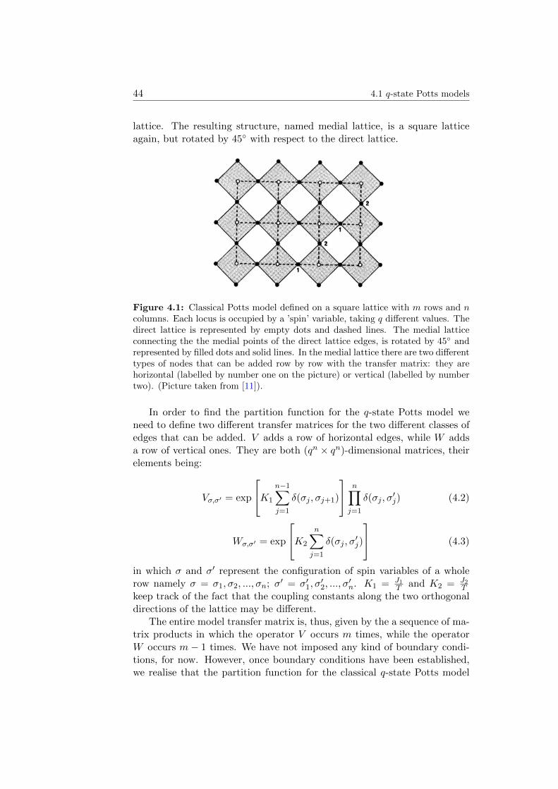
44 4.1 q-state Potts models
lattice. The resulting structure, named medial lattice, is a square latticeagain, but rotated by 45 with respect to the direct lattice.
Figure 4.1: Classical Potts model defined on a square lattice with m rows and ncolumns. Each locus is occupied by a ’spin’ variable, taking q different values. Thedirect lattice is represented by empty dots and dashed lines. The medial latticeconnecting the the medial points of the direct lattice edges, is rotated by 45 andrepresented by filled dots and solid lines. In the medial lattice there are two differenttypes of nodes that can be added row by row with the transfer matrix: they arehorizontal (labelled by number one on the picture) or vertical (labelled by numbertwo). (Picture taken from [11]).
In order to find the partition function for the q-state Potts model weneed to define two different transfer matrices for the two different classes ofedges that can be added. V adds a row of horizontal edges, while W addsa row of vertical ones. They are both (qn × qn)-dimensional matrices, theirelements being:
Vσ,σ′ = exp
K1
n−1∑j=1
δ(σj , σj+1)
n∏j=1
δ(σj , σ′j) (4.2)
Wσ,σ′ = exp
K2
n∑j=1
δ(σj , σ′j)
(4.3)
in which σ and σ′ represent the configuration of spin variables of a wholerow namely σ = σ1, σ2, ..., σn; σ′ = σ′1, σ
′2, ..., σ
′n. K1 = J1
T and K2 = J2T
keep track of the fact that the coupling constants along the two orthogonaldirections of the lattice may be different.
The entire model transfer matrix is, thus, given by the a sequence of ma-trix products in which the operator V occurs m times, while the operatorW occurs m− 1 times. We have not imposed any kind of boundary condi-tions, for now. However, once boundary conditions have been established,we realise that the partition function for the classical q-state Potts model
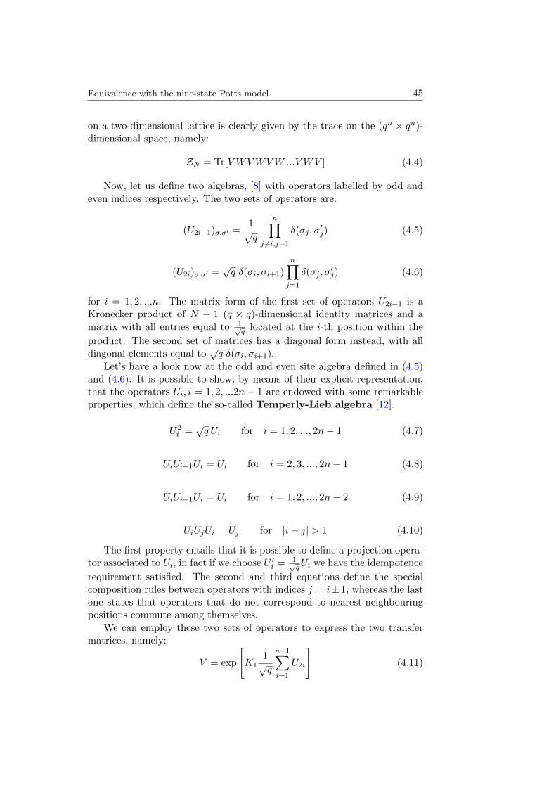
Equivalence with the nine-state Potts model 45
on a two-dimensional lattice is clearly given by the trace on the (qn × qn)-dimensional space, namely:
ZN = Tr[VWVWVW....V WV ] (4.4)
Now, let us define two algebras, [8] with operators labelled by odd andeven indices respectively. The two sets of operators are:
(U2i−1)σ,σ′ =1√q
n∏j 6=i,j=1
δ(σj , σ′j) (4.5)
(U2i)σ,σ′ =√q δ(σi, σi+1)
n∏j=1
δ(σj , σ′j) (4.6)
for i = 1, 2, ...n. The matrix form of the first set of operators U2i−1 is aKronecker product of N − 1 (q × q)-dimensional identity matrices and amatrix with all entries equal to 1√
q located at the i-th position within the
product. The second set of matrices has a diagonal form instead, with alldiagonal elements equal to
√q δ(σi, σi+1).
Let’s have a look now at the odd and even site algebra defined in (4.5)and (4.6). It is possible to show, by means of their explicit representation,that the operators Ui, i = 1, 2, ...2n − 1 are endowed with some remarkableproperties, which define the so-called Temperly-Lieb algebra [12].
U2i =√q Ui for i = 1, 2, ..., 2n− 1 (4.7)
UiUi−1Ui = Ui for i = 2, 3, ..., 2n− 1 (4.8)
UiUi+1Ui = Ui for i = 1, 2, ..., 2n− 2 (4.9)
UiUjUi = Uj for |i− j| > 1 (4.10)
The first property entails that it is possible to define a projection opera-tor associated to Ui, in fact if we choose U ′i = 1√
qUi we have the idempotence
requirement satisfied. The second and third equations define the specialcomposition rules between operators with indices j = i±1, whereas the lastone states that operators that do not correspond to nearest-neighbouringpositions commute among themselves.
We can employ these two sets of operators to express the two transfermatrices, namely:
V = exp
[K1
1√q
n−1∑i=1
U2i
](4.11)
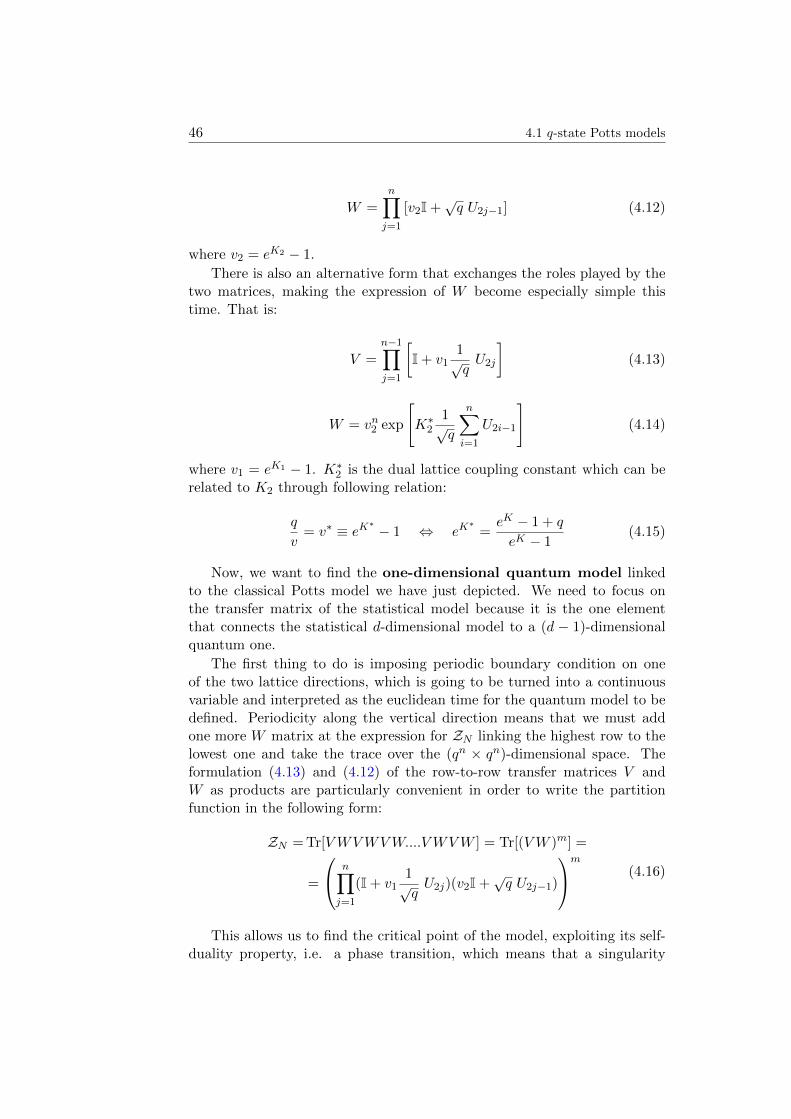
46 4.1 q-state Potts models
W =
n∏j=1
[v2I +√q U2j−1] (4.12)
where v2 = eK2 − 1.
There is also an alternative form that exchanges the roles played by thetwo matrices, making the expression of W become especially simple thistime. That is:
V =n−1∏j=1
[I + v1
1√qU2j
](4.13)
W = vn2 exp
[K∗2
1√q
n∑i=1
U2i−1
](4.14)
where v1 = eK1 − 1. K∗2 is the dual lattice coupling constant which can berelated to K2 through following relation:
q
v= v∗ ≡ eK∗ − 1 ⇔ eK
∗=eK − 1 + q
eK − 1(4.15)
Now, we want to find the one-dimensional quantum model linkedto the classical Potts model we have just depicted. We need to focus onthe transfer matrix of the statistical model because it is the one elementthat connects the statistical d-dimensional model to a (d − 1)-dimensionalquantum one.
The first thing to do is imposing periodic boundary condition on oneof the two lattice directions, which is going to be turned into a continuousvariable and interpreted as the euclidean time for the quantum model to bedefined. Periodicity along the vertical direction means that we must addone more W matrix at the expression for ZN linking the highest row to thelowest one and take the trace over the (qn × qn)-dimensional space. Theformulation (4.13) and (4.12) of the row-to-row transfer matrices V andW as products are particularly convenient in order to write the partitionfunction in the following form:
ZN = Tr[VWVWVW....V WVW ] = Tr[(VW )m] =
=
n∏j=1
(I + v11√qU2j)(v2I +
√q U2j−1)
m
(4.16)
This allows us to find the critical point of the model, exploiting its self-duality property, i.e. a phase transition, which means that a singularity
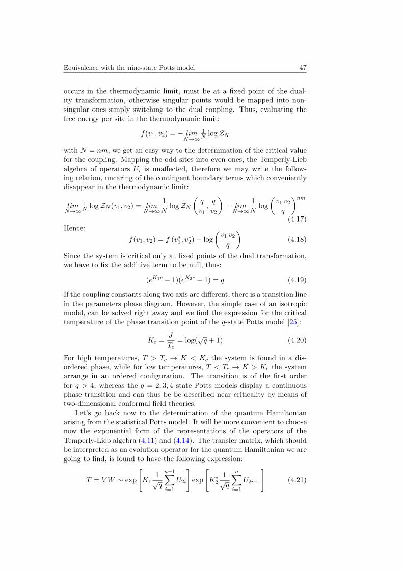
Equivalence with the nine-state Potts model 47
occurs in the thermodynamic limit, must be at a fixed point of the dual-ity transformation, otherwise singular points would be mapped into non-singular ones simply switching to the dual coupling. Thus, evaluating thefree energy per site in the thermodynamic limit:
f(v1, v2) = − limN→∞
1N logZN
with N = nm, we get an easy way to the determination of the critical valuefor the coupling. Mapping the odd sites into even ones, the Temperly-Liebalgebra of operators Ui is unaffected, therefore we may write the follow-ing relation, uncaring of the contingent boundary terms which convenientlydisappear in the thermodynamic limit:
limN→∞
1N logZN (v1, v2) = lim
N→∞
1
NlogZN
(q
v1,q
v2
)+ limN→∞
1
Nlog
(v1 v2q
)nm(4.17)
Hence:
f(v1, v2) = f (v∗1, v∗2)− log
(v1 v2q
)(4.18)
Since the system is critical only at fixed points of the dual transformation,we have to fix the additive term to be null, thus:
(eK1c − 1)(eK2c − 1) = q (4.19)
If the coupling constants along two axis are different, there is a transition linein the parameters phase diagram. However, the simple case of an isotropicmodel, can be solved right away and we find the expression for the criticaltemperature of the phase transition point of the q-state Potts model [25]:
Kc =J
Tc= log(
√q + 1) (4.20)
For high temperatures, T > Tc → K < Kc the system is found in a dis-ordered phase, while for low temperatures, T < Tc → K > Kc the systemarrange in an ordered configuration. The transition is of the first orderfor q > 4, whereas the q = 2, 3, 4 state Potts models display a continuousphase transition and can thus be be described near criticality by means oftwo-dimensional conformal field theories.
Let’s go back now to the determination of the quantum Hamiltonianarising from the statistical Potts model. It will be more convenient to choosenow the exponential form of the representations of the operators of theTemperly-Lieb algebra (4.11) and (4.14). The transfer matrix, which shouldbe interpreted as an evolution operator for the quantum Hamiltonian we aregoing to find, is found to have the following expression:
T = VW ∼ exp
[K1
1√q
n−1∑i=1
U2i
]exp
[K∗2
1√q
n∑i=1
U2i−1
](4.21)
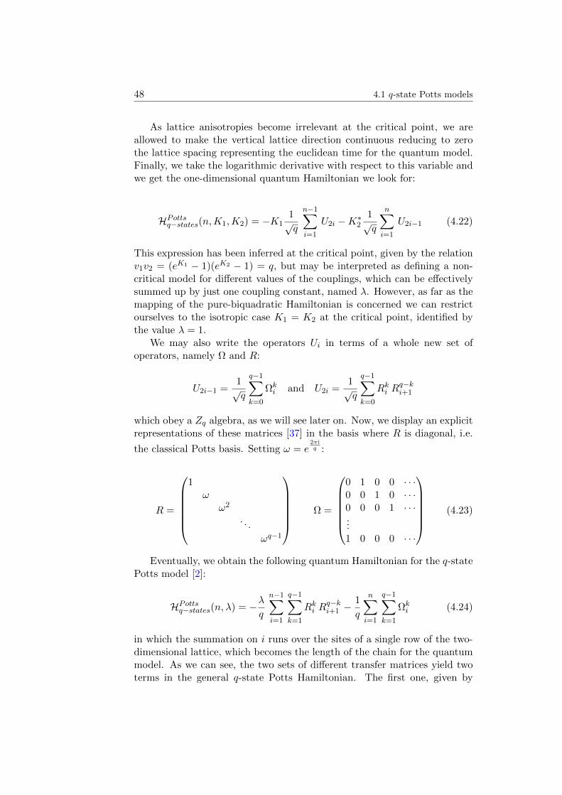
48 4.1 q-state Potts models
As lattice anisotropies become irrelevant at the critical point, we areallowed to make the vertical lattice direction continuous reducing to zerothe lattice spacing representing the euclidean time for the quantum model.Finally, we take the logarithmic derivative with respect to this variable andwe get the one-dimensional quantum Hamiltonian we look for:
HPottsq−states(n,K1,K2) = −K11√q
n−1∑i=1
U2i −K∗21√q
n∑i=1
U2i−1 (4.22)
This expression has been inferred at the critical point, given by the relationv1v2 = (eK1 − 1)(eK2 − 1) = q, but may be interpreted as defining a non-critical model for different values of the couplings, which can be effectivelysummed up by just one coupling constant, named λ. However, as far as themapping of the pure-biquadratic Hamiltonian is concerned we can restrictourselves to the isotropic case K1 = K2 at the critical point, identified bythe value λ = 1.
We may also write the operators Ui in terms of a whole new set ofoperators, namely Ω and R:
U2i−1 =1√q
q−1∑k=0
Ωki and U2i =
1√q
q−1∑k=0
Rki Rq−ki+1
which obey a Zq algebra, as we will see later on. Now, we display an explicitrepresentations of these matrices [37] in the basis where R is diagonal, i.e.
the classical Potts basis. Setting ω = e2πiq :
R =
1
ωω2
. . .
ωq−1
Ω =
0 1 0 0 · · ·0 0 1 0 · · ·0 0 0 1 · · ·...1 0 0 0 · · ·
(4.23)
Eventually, we obtain the following quantum Hamiltonian for the q-statePotts model [2]:
HPottsq−states(n, λ) = −λq
n−1∑i=1
q−1∑k=1
Rki Rq−ki+1 −
1
q
n∑i=1
q−1∑k=1
Ωki (4.24)
in which the summation on i runs over the sites of a single row of the two-dimensional lattice, which becomes the length of the chain for the quantummodel. As we can see, the two sets of different transfer matrices yield twoterms in the general q-state Potts Hamiltonian. The first one, given by
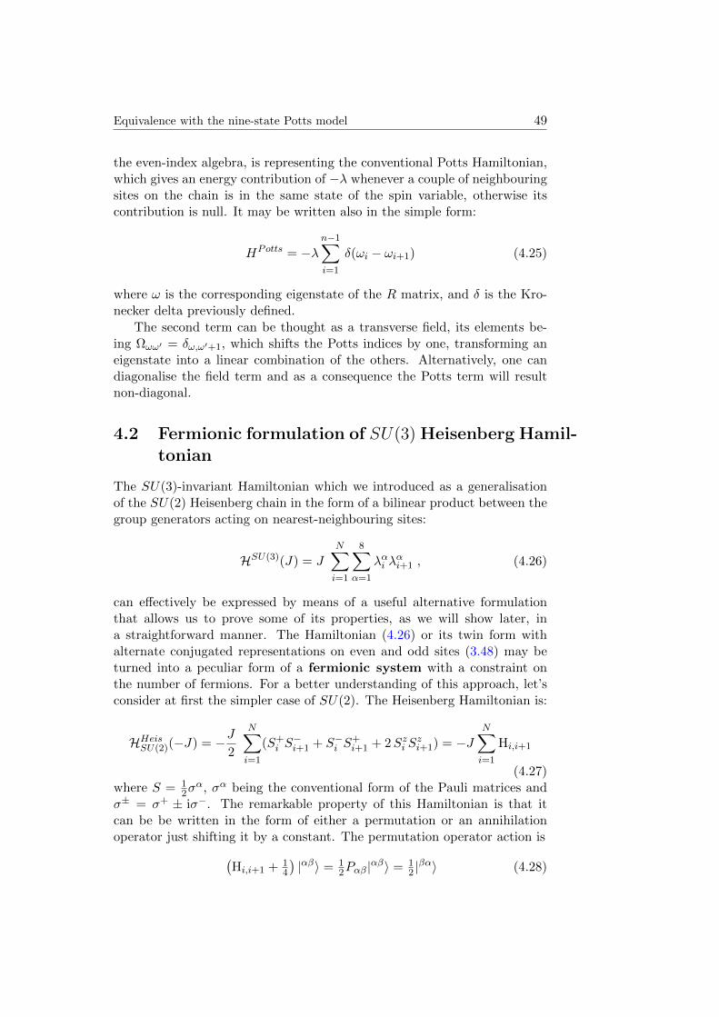
Equivalence with the nine-state Potts model 49
the even-index algebra, is representing the conventional Potts Hamiltonian,which gives an energy contribution of −λ whenever a couple of neighbouringsites on the chain is in the same state of the spin variable, otherwise itscontribution is null. It may be written also in the simple form:
HPotts = −λn−1∑i=1
δ(ωi − ωi+1) (4.25)
where ω is the corresponding eigenstate of the R matrix, and δ is the Kro-necker delta previously defined.
The second term can be thought as a transverse field, its elements be-ing Ωωω′ = δω,ω′+1, which shifts the Potts indices by one, transforming aneigenstate into a linear combination of the others. Alternatively, one candiagonalise the field term and as a consequence the Potts term will resultnon-diagonal.
4.2 Fermionic formulation of SU(3)Heisenberg Hamil-tonian
The SU(3)-invariant Hamiltonian which we introduced as a generalisationof the SU(2) Heisenberg chain in the form of a bilinear product between thegroup generators acting on nearest-neighbouring sites:
HSU(3)(J) = J
N∑i=1
8∑α=1
λαi λαi+1 , (4.26)
can effectively be expressed by means of a useful alternative formulationthat allows us to prove some of its properties, as we will show later, ina straightforward manner. The Hamiltonian (4.26) or its twin form withalternate conjugated representations on even and odd sites (3.48) may beturned into a peculiar form of a fermionic system with a constraint onthe number of fermions. For a better understanding of this approach, let’sconsider at first the simpler case of SU(2). The Heisenberg Hamiltonian is:
HHeisSU(2)(−J) = −J2
N∑i=1
(S+i S−i+1 + S−i S
+i+1 + 2Szi S
zi+1) = −J
N∑i=1
Hi,i+1
(4.27)where S = 1
2σα, σα being the conventional form of the Pauli matrices and
σ± = σ+ ± iσ−. The remarkable property of this Hamiltonian is that itcan be be written in the form of either a permutation or an annihilationoperator just shifting it by a constant. The permutation operator action is(
Hi,i+1 + 14
)|αβ〉 = 1
2Pαβ|αβ〉 = 12 |βα〉 (4.28)
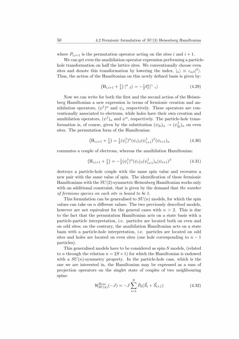
50 4.2 Fermionic formulation of SU(3) Heisenberg Hamiltonian
where Pi,i+1 is the permutation operator acting on the sites i and i+ 1.
We can get even the annihilation operator expression performing a particle-hole transformation on half the lattice sites. We conventionally choose evensites and denote this transformation by lowering the index, |α〉 ≡ εαβ|β〉.Thus, the action of the Hamiltonian on this newly defined basis is given by:(
Hi,i+1 + 14
)|α β〉 = −1
2δαβ |γ γ〉 (4.29)
Now we can write for both the first and the second action of the Heisen-berg Hamiltonian a new expression in terms of fermionic creation and an-nihilation operators, (ψ†)α and ψα respectively. These operators are con-ventionally associated to electrons, while holes have their own creation andannihilation operators, (ψ†)α and ψα, respectively. The particle-hole trans-
formation is, of course, given by the substitution (ψ2i)α → (ψ†2i)α on evensites. The permutation form of the Hamiltonian:(
Hi,i+1 + 14
)= 1
2(ψ†i )α(ψi)β(ψ†i+1)
β(ψi+1)α (4.30)
commutes a couple of electrons, whereas the annihilation Hamiltonian:(Hi,i+1 + 1
4
)= −1
2(ψ†i )α(ψi)β(ψ†i+1)α(ψi+1)
β (4.31)
destroys a particle-hole couple with the same spin value and recreates anew pair with the same value of spin. The identification of these fermionicHamiltonians with the SU(2)-symmetric Heisenberg Hamiltonian works onlywith an additional constraint, that is given by the demand that the numberof fermions species on each site is bound to be 1.
This formulation can be generalised to SU(n) models, for which the spinvalues can take on n different values. The two previously described models,however are not equivalent for the general cases with n > 2. This is dueto the fact that the permutation Hamiltonian acts on a state basis with aparticle-particle interpretation, i.e. particles are located both on even andon odd sites; on the contrary, the annihilation Hamiltonian acts on a statebasis with a particle-hole interpretation, i.e. particles are located on oddsites and holes are located on even sites (one hole corresponding to n − 1particles).
This generalised models have to be considered as spin-S models, (relatedto n through the relation n = 2S+ 1) for which the Hamiltonian is endowedwith a SU(n)-symmetry property. In the particle-hole case, which is theone we are interested in, the Hamiltonian may be expressed as a sum ofprojection operators on the singlet state of couples of two neighbouringspins:
HHeisSU(n)(−J) = −JN∑i=1
P0(~Si + ~Si+1) (4.32)
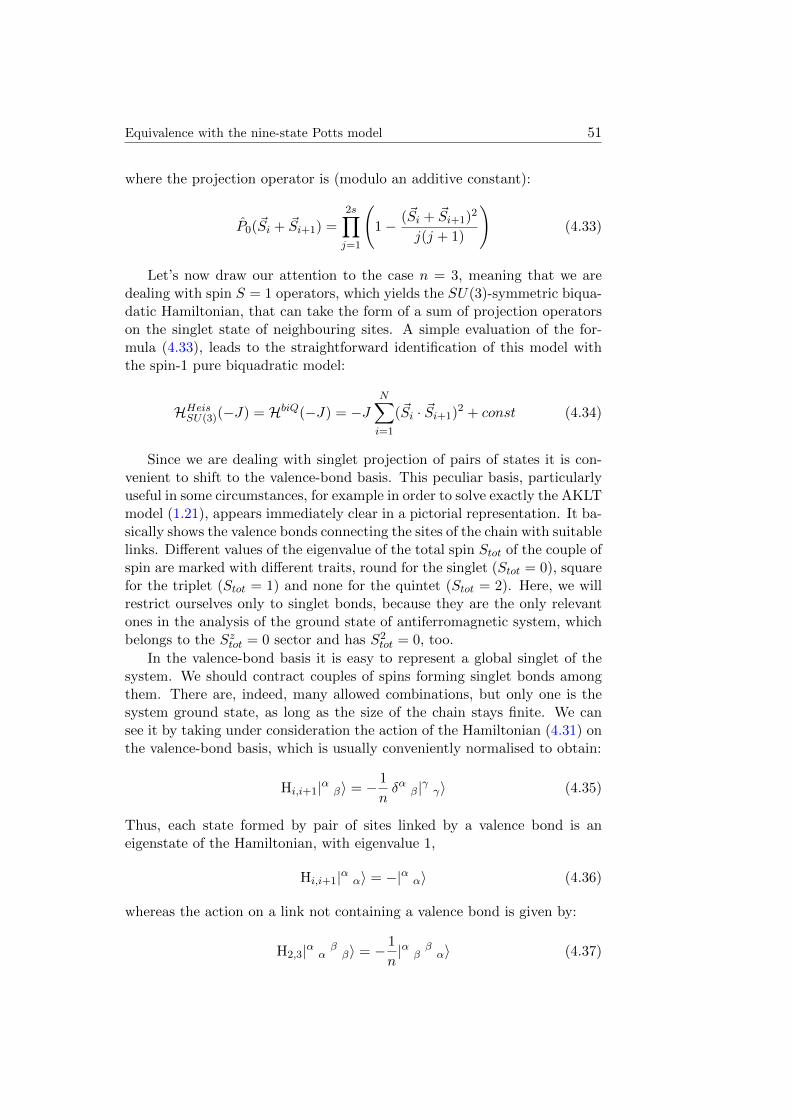
Equivalence with the nine-state Potts model 51
where the projection operator is (modulo an additive constant):
P0(~Si + ~Si+1) =
2s∏j=1
(1− (~Si + ~Si+1)
2
j(j + 1)
)(4.33)
Let’s now draw our attention to the case n = 3, meaning that we aredealing with spin S = 1 operators, which yields the SU(3)-symmetric biqua-datic Hamiltonian, that can take the form of a sum of projection operatorson the singlet state of neighbouring sites. A simple evaluation of the for-mula (4.33), leads to the straightforward identification of this model withthe spin-1 pure biquadratic model:
HHeisSU(3)(−J) = HbiQ(−J) = −JN∑i=1
(~Si · ~Si+1)2 + const (4.34)
Since we are dealing with singlet projection of pairs of states it is con-venient to shift to the valence-bond basis. This peculiar basis, particularlyuseful in some circumstances, for example in order to solve exactly the AKLTmodel (1.21), appears immediately clear in a pictorial representation. It ba-sically shows the valence bonds connecting the sites of the chain with suitablelinks. Different values of the eigenvalue of the total spin Stot of the couple ofspin are marked with different traits, round for the singlet (Stot = 0), squarefor the triplet (Stot = 1) and none for the quintet (Stot = 2). Here, we willrestrict ourselves only to singlet bonds, because they are the only relevantones in the analysis of the ground state of antiferromagnetic system, whichbelongs to the Sztot = 0 sector and has S2
tot = 0, too.
In the valence-bond basis it is easy to represent a global singlet of thesystem. We should contract couples of spins forming singlet bonds amongthem. There are, indeed, many allowed combinations, but only one is thesystem ground state, as long as the size of the chain stays finite. We cansee it by taking under consideration the action of the Hamiltonian (4.31) onthe valence-bond basis, which is usually conveniently normalised to obtain:
Hi,i+1|α β〉 = − 1
nδα β|γ γ〉 (4.35)
Thus, each state formed by pair of sites linked by a valence bond is aneigenstate of the Hamiltonian, with eigenvalue 1,
Hi,i+1|α α〉 = −|α α〉 (4.36)
whereas the action on a link not containing a valence bond is given by:
H2,3|α αββ〉 = − 1
n|α β
βα〉 (4.37)
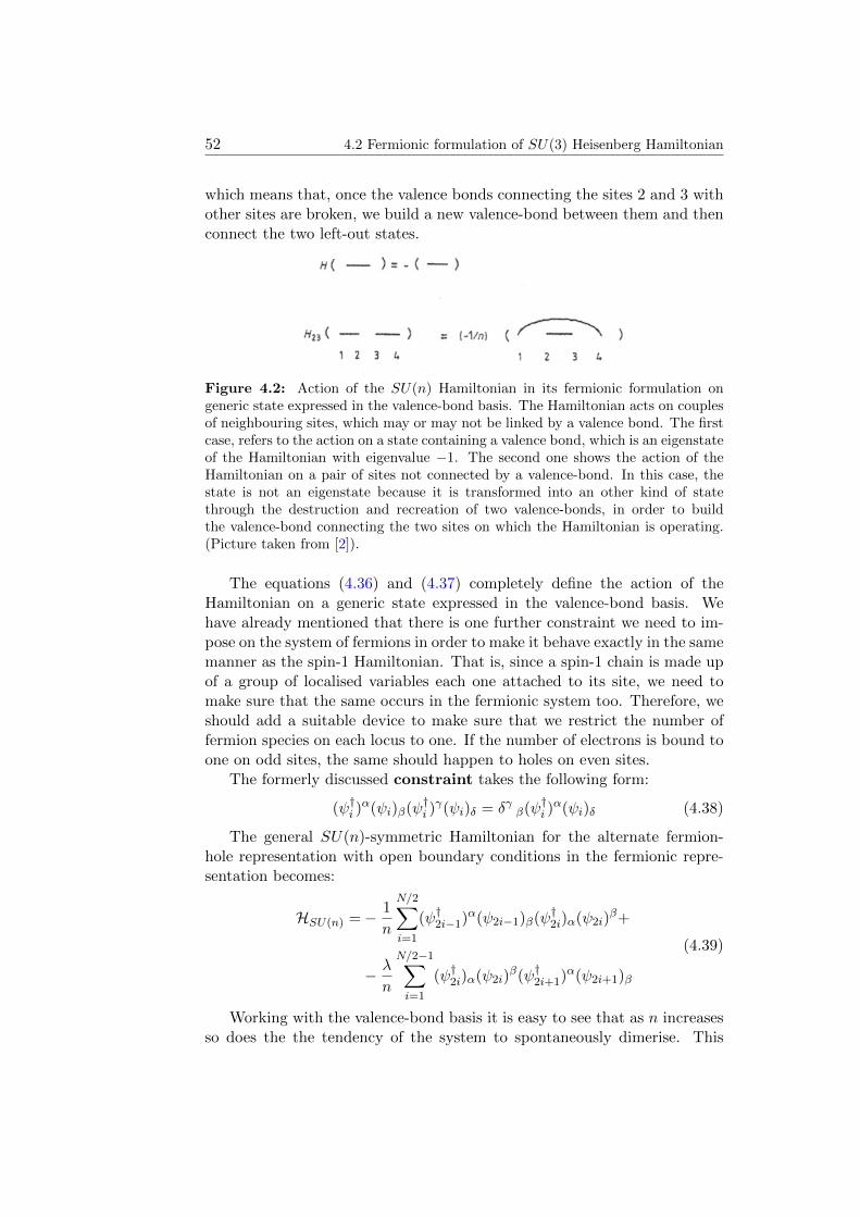
52 4.2 Fermionic formulation of SU(3) Heisenberg Hamiltonian
which means that, once the valence bonds connecting the sites 2 and 3 withother sites are broken, we build a new valence-bond between them and thenconnect the two left-out states.
Figure 4.2: Action of the SU(n) Hamiltonian in its fermionic formulation ongeneric state expressed in the valence-bond basis. The Hamiltonian acts on couplesof neighbouring sites, which may or may not be linked by a valence bond. The firstcase, refers to the action on a state containing a valence bond, which is an eigenstateof the Hamiltonian with eigenvalue −1. The second one shows the action of theHamiltonian on a pair of sites not connected by a valence-bond. In this case, thestate is not an eigenstate because it is transformed into an other kind of statethrough the destruction and recreation of two valence-bonds, in order to buildthe valence-bond connecting the two sites on which the Hamiltonian is operating.(Picture taken from [2]).
The equations (4.36) and (4.37) completely define the action of theHamiltonian on a generic state expressed in the valence-bond basis. Wehave already mentioned that there is one further constraint we need to im-pose on the system of fermions in order to make it behave exactly in the samemanner as the spin-1 Hamiltonian. That is, since a spin-1 chain is made upof a group of localised variables each one attached to its site, we need tomake sure that the same occurs in the fermionic system too. Therefore, weshould add a suitable device to make sure that we restrict the number offermion species on each locus to one. If the number of electrons is bound toone on odd sites, the same should happen to holes on even sites.
The formerly discussed constraint takes the following form:
(ψ†i )α(ψi)β(ψ†i )
γ(ψi)δ = δγ β(ψ†i )α(ψi)δ (4.38)
The general SU(n)-symmetric Hamiltonian for the alternate fermion-hole representation with open boundary conditions in the fermionic repre-sentation becomes:
HSU(n) =− 1
n
N/2∑i=1
(ψ†2i−1)α(ψ2i−1)β(ψ†2i)α(ψ2i)
β+
− λ
n
N/2−1∑i=1
(ψ†2i)α(ψ2i)β(ψ†2i+1)
α(ψ2i+1)β
(4.39)
Working with the valence-bond basis it is easy to see that as n increasesso does the the tendency of the system to spontaneously dimerise. This
Equivalence with the nine-state Potts model 53
happens because the contribution of the valence-bond breaking term (4.37)of the Hamiltonian become less important as n → ∞, as its amplitude hasa 1n behaviour. Therefore, the dimerised state, in which odd-even pairs of
neighbouring sites connecting 2i − 1 to 2i with a singlet bond create N/2alternate bonds on the N allowed lattice spaces of the chain, is the exactground state in the large n limit. The lowest energy configuration is thusthe following one, with contributions coming just from the valence-bonds:
HHeisSU(n)|α αββγγ ...〉 =
N∑i=1
Hi,i+1|α αββγγ ...〉 = −N
2|α α
ββγγ ...〉
(4.40)
In fact, all off-diagonal terms contributions in the Hamiltonian operatorsare of order O
(1n
). The other singlet states with non-nearest neighbour
bonds have an energy gap of 1 +O(1n
)and non-singlet states, with missing
bonds (uncontracted indices) have at least an equal gap.
Reminding that we keep on working with periodic boundary conditions,in the infinite volume limit, if we impose on the system periodic boundaryconditions, the ground state becomes doubly degenerate, because there aretwo equally probable configurations connected one to another by a transla-tion of all bonds by one lattice constant.
4.3 Correspondence between the Potts model andthe biquadratic Hamiltonian
The whole purpose of the interpretation in terms of fermionic operators ofthe pure-biquadratic Hamiltonian was to exploit this formulation to provethe equivalence between the former and and the quantum version of thenine-state Potts model. The Hamiltonian version of the latter should bepossible only at the critical point, defined by (4.20). However, uncaringof the lattice anisotropy, we could take the continuum limit in one of thetwo dimensions of the rectangular two-dimensional lattice of the statisticalmodel depicted in section 4.1. Identifying this direction with the time axis,we get the one-dimensional quantum Hamiltonian of the q-state Potts modelnear the critical point, which has the following expression:
HPottsq−states(L, λ) = −λq
L−1∑i=1
q−1∑k=1
Rki Rq−ki+1 −
1
q
L∑i=1
q−1∑k=1
Ωki (4.41)
for which the critical point corresponds to the critical value of the parameterλ = 1.
We are now on the edge of showing that the biquadratic Hamiltonianmay be written in an identical form thanks to the realisation that we can
54 4.3 Correspondence between the Potts model and the biquadratic Hamiltonian
build a Temperly-Lieb algebra of its operators too. Let us start from theHamiltonian in the most general form:
HbiQ(−J) =− JN−1∑i=1
εi(~Si · ~Si+1)2 = −J
[N−1∑i=1
εi (hi + 1)
](4.42)
where εi takes different values on even and odd sites, namely ε2i+1 = 1and ε2i = λ, as a measure of the dimerisation tendency of the system.There is one other significant difference from the conventional form of theHamiltonian used so far: there is in fact one less term in the summationover all sites, due to the choice to deal with open boundary conditions, i.e~SN+1 = 0.
We stated previously that the operators hi satisfy the relation h2i = 3hi.
This is just one of the characteristic features of the operators hi. It maybe shown that they fulfill all the requirements of the Temperly-Lieb algebradefinition, namely:
h2i = 3 hi for i = 1, 2, ..., N (4.43)
hi hi−1 hi = hi for i = 2, 3, ..., N (4.44)
hi hi+1 hi = hi for i = 1, 2, ..., N − 1 (4.45)
hi hj hi = hj for |i− j| > 1 (4.46)
which resemble exactly the relations (4.7), (4.8), (4.9) and (4.10) with√q =
3 and 2n = N . These are the first signals that the pure biquadratic spin-1Hamiltonian may be connected to a Potts model with q = 9 states definedon a chain of half the length of the biquadratic one.
Right now, let’s proceed by proving that these relations, in fact, hold. Itwill be really easy to achieve our goal if we make use of the newly introducedrepresentation in terms of fermionic operators. It should be noticed that thehi operators are not different from the operators:
Hi,i+1 = −13(ψ†i )
α(ψi)β(ψ†i+1)α(ψi+1)β (4.47)
which act according to (4.35) for n = 3, which means S = 1. We can startwith the first relation, which we can, by the way, check out even from itsexplicit representation (2.31). Making extensive use of the constraint of one
Equivalence with the nine-state Potts model 55
particle (or hole) per site (4.38), we get:
h2i =
1
9
((ψ†i )
α(ψi)β(ψ†i+1)α(ψi+1)β)(
(ψ†i )γ(ψi)δ(ψ
†i+1)γ(ψi+1)
δ)
=
=1
9
((ψ†i )
α(ψi)β(ψ†i )γ(ψi)δ)(
(ψ†i+1)α(ψi+1)β(ψ†i+1)γ(ψi+1)
δ)
=
=1
9
(δγ β(ψ†i )
α(ψi)δ
)(δβ γ(ψ†i+1)α(ψi+1)
δ)
=
=31
9(ψ†i )
α(ψi)δ(ψ†i+1)α(ψi+1)
δ) = 3 hi
(4.48)
Let’s deal with the second and third relation, which may be treated exactlyin the same way:
hi hi+1 hi =− 1
27
((ψ†i )
α(ψi)β(ψ†i+1)α(ψi+1)β)(
(ψ†i+1)γ(ψi+1)δ(ψ†i+2)
γ(ψi+2)δ
)(
(ψ†i )ε(ψi)η(ψ
†i+1)ε(ψi+1)
η)
=
=− 1
27
(δβ
ε(ψ†i )α(ψi)ν
)(δδ ε δ
βγ(ψ†i+1)α(ψi+1)
ν)(
(ψ†i+2)γ(ψi+2)δ
)=
=− 31
27
((ψ†i )
α(ψi)ν
)((ψ†i+1)α(ψi+1)
ν)(
(ψ†i+2)γ(ψi+2)γ
)=
=− 1
3
((ψ†i )
α(ψi)ν(ψ†i+1)α(ψi+1)ν)
= hi
(4.49)
Eventually, the third relation it is clearly inferred from the former one: ifthere are fermionic operators involved with two or more lattice sites of dis-tance, they obviously have not any common indices, thus they all commuteamong themselves.
Once the properties of the Temperly-Lieb algebra have been proved, wemay connect the spin operators hi to the odd and even algebras of the corre-sponding Potts model. We will finally reach a formulation of the biquadraticHamiltonian equivalent to the nine-state Potts model. It is sufficient to makethe identifications hi = Hi,i+1 = Ui for i = 1, 2..., 2n(= N).
According to [9], we should define the two usual odd and even algebrasof the Potts model employing the hi = Ui operators, which are divided intwo classes:
h2i−1 =1√q
q−1∑k=0
Ωki and h2i =
1√q
q−1∑k=0
Rki Rq−ki+1 (4.50)
with i = 1, 2, ...N/2 for the odd part of the algebra and i = 1, 2, ...N/2 − 1for the even part of the algebra. This distinction is due to the fact that wechose to work in the open boundary conditions framework (thus, hN = 0),which makes easier the proof of the equivalence between the two modelsunder examination.
56 4.3 Correspondence between the Potts model and the biquadratic Hamiltonian
These new sets of operators on each site form a Zq algebra, with thefollowing commutation rules:
ΩiRi = ω−1RiΩi , ΩiR†i = ωR†iΩi and Ωq
i = Rqi = 1 (4.51)
where we have defined ω = e2πiq .
Now, from the comparison between the relation (4.43) on the square ofthe hi operators and the general property (4.7), we realise that q = 9, thusthe biquadratic Hamiltonian turns out to be related to a nine-state Pottsmodel, with its odd- and even-site operators obeying the Temperly-Liebalgebra. Therefore, making use of the substitutions (4.50), we can write:
1JHbiQ(−J) = −
N−1∑i=1
εi (hi + 1) =
= −
N/2∑i=1
h2i−1 + λ
N/2−1∑i=1
h2i + 12N + λ(12N − 1)
=
= −(
1√q
L∑i=1
q−1∑k=0
Ωki + 1√
q λ
L−1∑i=
q−1∑k=0
Rki Rq−ki+1 + L+ λ(L− 1)
)=
= −(
13
L∑i=1
8∑k=1
Ωki + 1
3 λL−1∑i=
8∑k=1
Rki R9−ki+1 + 4
3L+ 43λ(L− 1)
)=
= 3HPotts9−states(L, λ)− 43L− 4
3λ(L− 1)
(4.52)
where in the third line we defined L = N/2 and in the fourth line we usedthe properties of the Z9 algebra, according to which Ω9 = R9 = 1. We havethus shown that there is indeed an equivalence between the spin-1 antifer-romagnetic pure biquadratic model and the one-dimensional quantumHamiltonian of the nine-state Potts model. This correspondence holdsthanks to the common underlying algebra of operators characterising bothmodels, that is the Temperly-Lieb algebra, provided that we work under thepremise of open boundary conditions.
Knowing that the spin-1 pure biquadratic model was also partially mappedinto a spin-1/2 XXZ chain (see section 2.1 for further details), we may havea representation of the Temperly-Lieb algebra also in terms of the spin-1/2operators, i.e the Pauli matrices. That is:
Ui =1
2(σxi σ
xi+1+σyi σ
yi+1)+
1
2cosh θ(1−σzi σzi+1)−
1
2sinh θ(σzi −σzi+1) (4.53)
where the correspondence with the Temperly-Lieb algebra (4.7), (4.8), (4.9)and (4.10) is recovered if we set 2 cosh θ =
√q. Hence we find that the
biquadratic Hamiltonian with open boundary conditions is related to the
Equivalence with the nine-state Potts model 57
spin-1/2 XXZ model by the following equivalence relation. (For simplicity,we will restrict our calculation to the case λ = 1.)
1
JHbiQ(−J,N) = −
N−1∑i=1
Ui − (N − 1) =
= −N−1∑i=1
[1
2(σxi σ
xi+1 + σyi σ
yi+1) +
1
2cosh θ(1− σzi σzi+1)−
1
2sinh θ(σzi − σzi+1)
]+
− (N − 1) =
= −1
2
N−1∑i=1
[σxi σ
xi+1 + σyi σ
yi+1 − cosh θσzi σ
zi+1
]+
1
2sinh θ(σz1 − σzN )+
−(
1 +cosh θ
2
)(N − 1)
(4.54)
Comparing the former expression to the conventional form of the spin-1/2XXZ Hamiltonian:
HXXZ(J) =1
2J
N∑i=1
[σxi σ
xi+1 + σyi σ
yi+1 + ∆σzi σ
zi+1
](4.55)
we realise that our spin-1 biquadratic Hamiltonian is equivalent to an an-tiferromagnetic model (negative coupling), defined on a chain of length N ,with free ends (summation running to N − 1), its anistoropy parameter
being ∆ = − cosh θ = −√q2 = −3
2 . Furthermore, external fields of values
±p2 = ± sinh θ
2 =√52 are applied to the extremes of the chain. Therefore the
correspondence we have established is:
1
JHbiQ(−J,N) = HXXZspin−1/2(N,∆ = 3
2 ,±p = ±√52 ) (4.56)
This model was solved for the general case in [6] via the Bethe ansatz tech-nique, which yields:
EXXZ = −1
2(N − 1)∆− 2
n∑j=1
(cos kj −∆) (4.57)
with the quasi-momenta kj bound to be solutions of the Bethe ansatz equa-tions [9]:
k2Nj =
n∏l 6=j=1
S(kl, kj)S(k−1l , kj)
S(kj , jkl)S(kj , k−1l )
, j = 1, 2, ...n (4.58)
where S(kl, kj) = 1 + 2∆kj + kjkl.
58 4.3 Correspondence between the Potts model and the biquadratic Hamiltonian
From the explicit form of the energy eigenvalues and knowing the valuesof the parameters which allow the mapping, we can recover information bothon the nine-state Potts model and on the spin-1 biquadratic Hamiltonianfrom which we started. All of the three are mapped one into another withelementary modifications, such as the introduction of a scaling factor andaddtitive constants, which do not alter the spectrum of the model but simplyshift and rescale it. Here is the complete equivalence:
HPotts9−states(L, λ = 1, free ends) ∼ HbiQspin−1(2L, λ = 1, free ends) ∼∼ HXXZspin−1/2(2L,∆ = 3
2 ,±p = ±√52 )
(4.59)
The allowed eigenvalues of the three models, are strictly related to theTemperly-Lieb algebra operators, therefore they must be the same set for allof the three models, however the degeneracies may not coincide due to thedifference in the dimensions of the representations chosen for the same op-erator algebra. Both the spin-1 biquadratic and the nine-state Potts modelhave the same dimension of the Hilbert-space of states, namely 32L×32L and9L × 9L respectively, whereas the XXZ spin-1/2 model has a smaller spaceof states which is 22L × 22L dimensional. This matter has been previouslydiscussed in section 2.4.
We stress once again the importance of the connection between the nine-state Potts model and the XXZ model, condensed in the relation ∆ =
cosh θ =√q2 . From this point of view we may get an explanation of the
different behaviour of the Potts model at phase transition point for q ≤ 4and q > 4. In the former case, corresponding to 0 < cosh θ ≤ 1, in the XXZinterpretation of the model we are going toward the XX-like behaviour,which is located in the massless region of the phase diagram (−1 ≤ ∆ < 0);while in the latter case, cosh θ > 1, which means we are going towards anIsing anisotropy (∆ < −1) and we are in the gapped region of the phasediagram.
The nine-state Potts model shows a first order phase transition in thethermodynamic limit, which means that its related quantum Hamiltonian atthe critical point λ = 1 undergoes an ordered-disoredered phase transition.In the low-temperature phase (λ > 1) the ground state is supposed to benine-fold degenerate. However, when dealing with finite size chains, thesymmetry is partially broken resulting in a splitting of the eigenvalues ina two sectors, distinguished by the eigenvalues of Ω [9]. The value ω = 0is singled out and the eight left eigenvalues remain still degenerate. This8 + 1 splitting reminds us of the SU(3) multiplet structure of the lowesteigenstates of the biquadratic Hamiltonian which presents a singlet and anoctet representation as its lowest energy states (open boundary conditions).Hence, for the nine-state Potts model (q > 4) there is a gap between theground and the first excited state, which is consistent with the fact that the
Equivalence with the nine-state Potts model 59
pure biquadratic Hamiltonian is located in a gapped region of the bilinear-biquadratic phase diagram (fig. 1.1).
This discussion may be extended to encompass even the generic SU(n)-symmetric system in its fermionic formulation (4.39). The equivalence withthe q-state Potts model is obvious for the n case too, since the fermionoperators were shown to be fulfilling the Temperly-Lieb algebra rules, withn =
√q. For q > 4, which means n > 2 the first order phase transition
guarantees that there are two distinct but coexisting ground states, oneordered and one disordered, which can be mapped one into the other at thecritical point (λ = 1) . Therefore, for n > 2 in the infinite volume limit, theground state is going to be doubly-degenerate meaning that the system isspontaneously dimerised, with its translational symmetry broken.
This does not occur for the case n ≤ 2, i.e. q ≤ 4, because the phasetransition is now continuous and the ground state is unique. This behaviouris confirmed by the SU(2) chain, which is the usual spin-1/2 Heisenbergmodel, solvable via the Bethe ansatz and having an undimerised and trans-lationally invariant ground state with a zero energy gap [40].
Concluding, it is important to recall that the equivalence of the spin-1biquadratic Hamiltonian with the Potts model is strictly connected to thechoice of free ends for both models, which leads to a correspondence withthe spin-1/2 XXZ chain previously described, having two opposite externalfields applied to the extremes. This might be a problem because in theprevious chapters we focused our discussion on periodic boundary conditionsonly and there is no guarantee that changing the conditions at the extremeswould not affect the behaviour of the model.
In particular, choosing periodic boundary conditions in this case leadsto a different version of the XXZ spin chain with a defect seam (yieldingtwisted boundary conditions), which is much more complicated to solve withthe Bethe ansatz. As long as the system size remains finite the gap of thebiquadratic Hamiltonian is also affected. However, while approaching thethermodynamic limit the discrepancy introduced by the change of boundaryconditions must become irrelevant. This statement [9] appears to be con-firmed by numerical results, which means that the gap of the biquadraticspin-1 chain in the thermodynamic limit is precisely given by the gap of theof the spin-1/2 XXZ chain in the thermodynamic limit calculated in [16].
4.4 q-state vertex models correspondence with thebiquadratic Hamiltonian
A different approach to the correspondence between the spin-1 pure bi-quadratic model and the Potts model was proposed by Klumper [27, 28].In order to connect this equivalence to the others previously examined weneed one further passage, that is the the discovered correspondence between
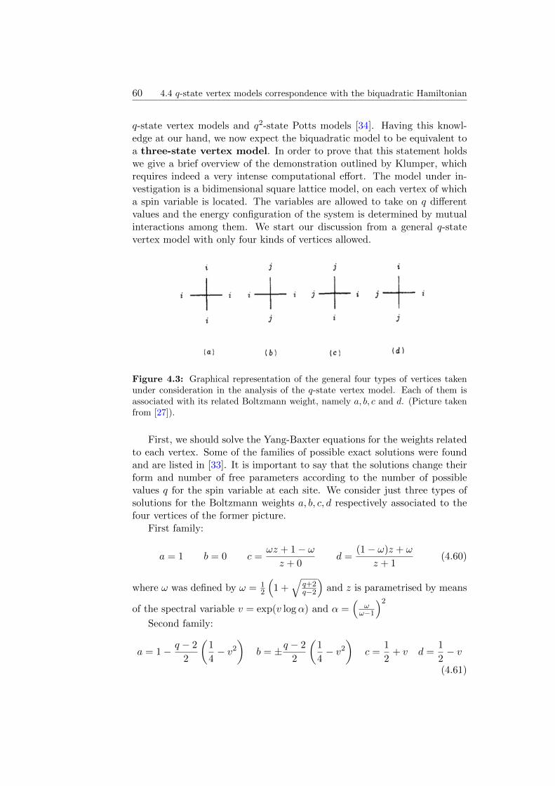
60 4.4 q-state vertex models correspondence with the biquadratic Hamiltonian
q-state vertex models and q2-state Potts models [34]. Having this knowl-edge at our hand, we now expect the biquadratic model to be equivalent toa three-state vertex model. In order to prove that this statement holdswe give a brief overview of the demonstration outlined by Klumper, whichrequires indeed a very intense computational effort. The model under in-vestigation is a bidimensional square lattice model, on each vertex of whicha spin variable is located. The variables are allowed to take on q differentvalues and the energy configuration of the system is determined by mutualinteractions among them. We start our discussion from a general q-statevertex model with only four kinds of vertices allowed.
Figure 4.3: Graphical representation of the general four types of vertices takenunder consideration in the analysis of the q-state vertex model. Each of them isassociated with its related Boltzmann weight, namely a, b, c and d. (Picture takenfrom [27]).
First, we should solve the Yang-Baxter equations for the weights relatedto each vertex. Some of the families of possible exact solutions were foundand are listed in [33]. It is important to say that the solutions change theirform and number of free parameters according to the number of possiblevalues q for the spin variable at each site. We consider just three types ofsolutions for the Boltzmann weights a, b, c, d respectively associated to thefour vertices of the former picture.
First family:
a = 1 b = 0 c =ωz + 1− ωz + 0
d =(1− ω)z + ω
z + 1(4.60)
where ω was defined by ω = 12
(1 +
√q+2q−2
)and z is parametrised by means
of the spectral variable v = exp(v logα) and α =(
ωω−1
)2Second family:
a = 1− q − 2
2
(1
4− v2
)b = ±q − 2
2
(1
4− v2
)c =
1
2+ v d =
1
2− v
(4.61)
Equivalence with the nine-state Potts model 61
Third family:
a = 1 b = 0 c =
√q − 1 z − 1
q − 2d =
√q − 1 z−1 − 1
q − 2(4.62)
where z = exp(v log(q − 1))The symmetry of the transfer matrices in the cases one and two (with
minus sign) is SO(q), while for the other cases the maximal symmetry istrivially the identity.
Once we have found these parametrised families of solutions for theBoltzmann weights, we need to find the explicit expression of the row-to-row tranfer matrix. This operation was performed thanks to some usefulsymmetry properties of the transfer matrix:
• symmetry relation: T †(v) = T (−v∗) → Λ∗(v) = Λ(−v∗)
• commutativity: T (v)T (v′) = T (v′)T (v)
• inversion relation: T (v)T (v + 1) = φ(v)N I +O(e−N ) →Λ(v)Λ(v + 1) = φ(v)N +O(e−N )
The third and most important property strictly holds just for the pointsv = ±1
2 , for which the transfer matrix becomes basically the right or leftshift operator. Since these matrices are inverse one of the other, we areallowed to write the inversion relation and we expect it to hold also in theneighbourhood of those points.
Then, we should proceed by computing the function φ for the threedifferent families, each one having its own characteristic expression, andexploiting the inversion relation, we may finally be able to find the partitionfunction per site. We should pay attention to the analytical properties ofthe functions we are dealing with. They have to be meromorphic in theanalytical region, i.e. −1
2 ≤ Re(v) ≤ 12 , and must satisfy required periodicity
or asimptotic behaviour to be well defined . We can then use an ansatz forthe partition function based on the previously mentioned properties andfinally get its explicit form exploiting the inversion relation.
We have to turn the statistical q-state vertex model into a one-dimensionalquantum model. This is done by taking the logarithmic derivative of thetransfer matrix at the shift point (v = −1
2), which ensures that the resultingHamiltonian is a local operator, i.e. the usual sum over operators acting onpairs of neighbouring sites.
Eventually we obtain two remarkable Hamiltonian expressions for thetwo mentioned families endowed with more symmetry properties (1 and2−). The first set of Boltzmann weights results in the following form:
H(1) = −2ω − 1
q2 − 4logα
N∑i=1
[(~Si · ~Si+1)2 − q + 1] (4.63)
62 4.4 q-state vertex models correspondence with the biquadratic Hamiltonian
where ~S = S1, S2, S3 are the generators of the group SO(q). The maxi-mal symmetry group of this Hamiltonian is, however, SL(q), which is largerthan SO(q) and contains also the special case SU(q), that for q = 3 re-produces the SU(3) symmetry which we already know to characterise thebiquadratic model.
Starting form the second one, choosing the minus sign and selecting thevalue q = 3, we obtain a Hamiltonian reproducing exactly the Takhtajan-Babujian model (1.11):
H(2−) =1
2(q − 2)
N∑i=1
[(q − 2)2(~Si · ~Si+1) + (q − 4)(~Si · ~Si+1)2 + q] (4.64)
This class of solutions is known to have a SO(q) maximal symmetry group,which is consistent with what we already know from the bilinear-biquadraticmodel at Θ = π
4 is not endowed with any more symmetry than the usualSU(2).
Chapter 5
Two-site, four-site andsix-site biquadraticHamiltonian
In the former chapters we have worked to find a set of good quantum num-bers for the biquadratic model both in its SU(2)-symmetric formulation, interms of spin-1 operators, and in its SU(3)-symmetric one, with Gell-Mannmatrices as group generators.
Now, it is about time to start a classification of the eigenstates accordingto these two different points of view. In the SU(2)-symmetric approach, wemay label the eigenstates according to eigenvalue Sztot, which is the onlygood quantum number immediately available to classify the states obtainedvia the Bethe ansatz technique (see 2.3). In this framework states are, thus,labelled with a number of deviations from the ferromagnetic ground state(the fully aligned one), which is, in fact, the highest excited state for thepure-biquadratic antiferromagnetic model.
We have developed also a different approach exploiting the SU(3)-symme-try properties of the Heisenberg chain, which led to a fundamental equiva-lence:
HF⊗A(J) = −2J
N∑i=1
(~Si · ~Si+1)2 +
8
3JN
provided Sx2i → −Sx2i and Sz2i → −Sz2i
(5.1)
Relying on this equivalence, we realise that there may be two good quan-tum numbers for the biquadratic Hamiltonian, which we have proved to beendowed with a SU(3) symmetry. They are:
63
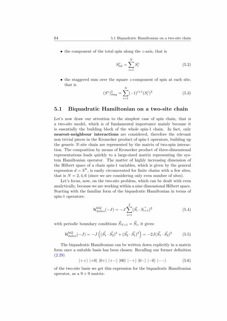
64 5.1 Biquadratic Hamiltonian on a two-site chain
• the component of the total spin along the z-axis, that is
Sztot =
N∑i=1
Szi (5.2)
• the staggered sum over the square z-component of spin at each site,that is
(Sz)2stag =
N∑i=1
(−1)i+1(Szi )2 (5.3)
5.1 Biquadratic Hamiltonian on a two-site chain
Let’s now draw our attention to the simplest case of spin chain, that isa two-site model, which is of fundamental importance mainly because itis essentially the building block of the whole spin-1 chain. In fact, onlynearest-neighbour interactions are considered, therefore the relevantnon trivial pieces in the Kronecker product of spin-1 operators, building upthe generic N -site chain are represented by the matrix of two-spin interac-tion. The composition by means of Kronecker product of three-dimensionalrepresentations leads quickly to a large-sized matrix representing the sys-tem Hamiltonian operator. The matter of highly increasing dimension ofthe Hilbert space of a chain spin-1 variables, which is given by the generalexpression d = 3N , is easily circumvented for finite chains with a few sites,that is N = 2, 4, 6 (since we are considering only even number of sites).
Let’s focus, now, on the two-site problem, which can be dealt with evenanalytically, because we are working within a nine dimensional Hilbert space.Starting with the familiar form of the biquadratic Hamiltonian in terms ofspin-1 operators:
HbiQ2sites(−J) = −J2∑i=1
(~Si · ~Si+1)2 (5.4)
with periodic boundary conditions ~SN+1 = ~S1, it gives:
HbiQ2sites(−J) = −J(
( ~S1 · ~S2)2 + ( ~S2 · ~S1)2)
= −2J( ~S1 · ~S2)2 (5.5)
The biquadratic Hamiltonian can be written down explicitly in a matrixform once a suitable basis has been chosen. Recalling our former definition(2.29)
|++〉 |+0〉 |0+〉 |+−〉 |00〉 |−+〉 |0−〉 |−0〉 |−−〉 (5.6)
of the two-site basis we get this expression for the biquadratic Hamiltonianoperator, as a 9× 9 matrix:
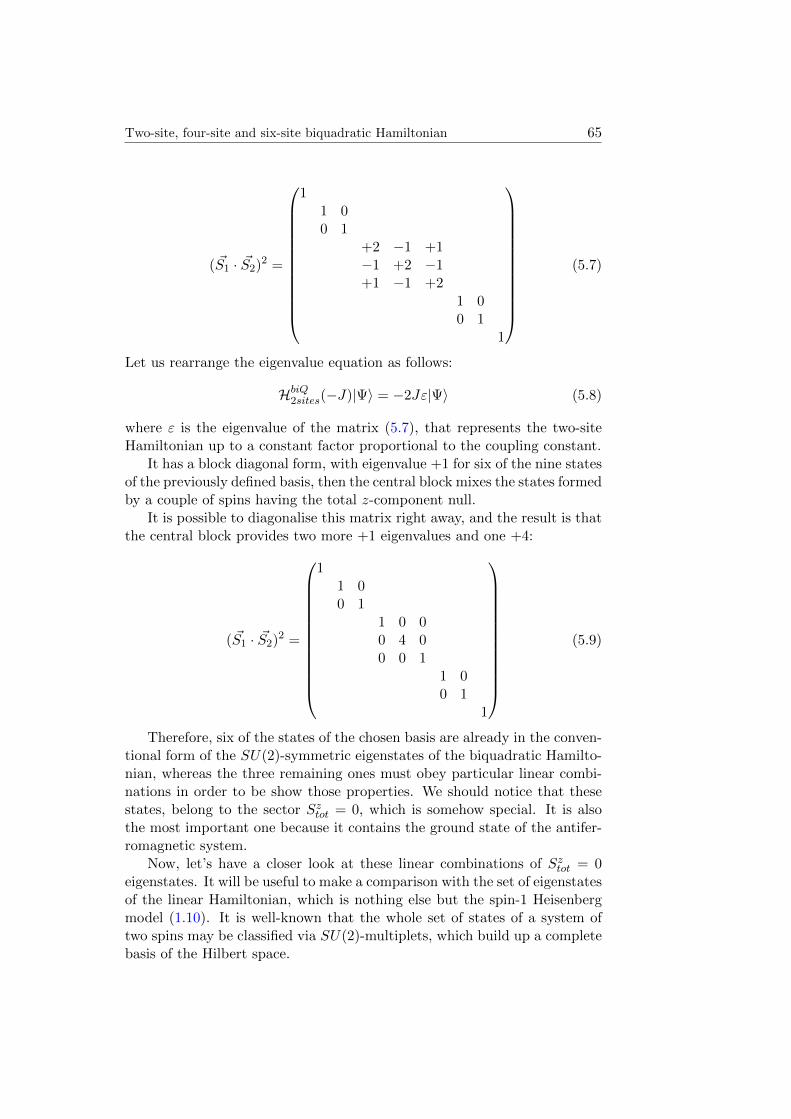
Two-site, four-site and six-site biquadratic Hamiltonian 65
( ~S1 · ~S2)2 =
11 00 1
+2 −1 +1−1 +2 −1+1 −1 +2
1 00 1
1
(5.7)
Let us rearrange the eigenvalue equation as follows:
HbiQ2sites(−J)|Ψ〉 = −2Jε|Ψ〉 (5.8)
where ε is the eigenvalue of the matrix (5.7), that represents the two-siteHamiltonian up to a constant factor proportional to the coupling constant.
It has a block diagonal form, with eigenvalue +1 for six of the nine statesof the previously defined basis, then the central block mixes the states formedby a couple of spins having the total z-component null.
It is possible to diagonalise this matrix right away, and the result is thatthe central block provides two more +1 eigenvalues and one +4:
( ~S1 · ~S2)2 =
11 00 1
1 0 00 4 00 0 1
1 00 1
1
(5.9)
Therefore, six of the states of the chosen basis are already in the conven-tional form of the SU(2)-symmetric eigenstates of the biquadratic Hamilto-nian, whereas the three remaining ones must obey particular linear combi-nations in order to be show those properties. We should notice that thesestates, belong to the sector Sztot = 0, which is somehow special. It is alsothe most important one because it contains the ground state of the antifer-romagnetic system.
Now, let’s have a closer look at these linear combinations of Sztot = 0eigenstates. It will be useful to make a comparison with the set of eigenstatesof the linear Hamiltonian, which is nothing else but the spin-1 Heisenbergmodel (1.10). It is well-known that the whole set of states of a system oftwo spins may be classified via SU(2)-multiplets, which build up a completebasis of the Hilbert space.
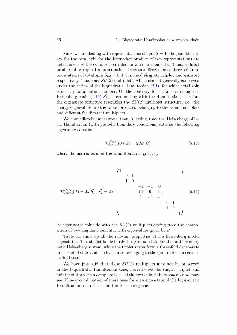
66 5.1 Biquadratic Hamiltonian on a two-site chain
Since we are dealing with representations of spin S = 1, the possible val-ues for the total spin for the Kronecker product of two representations aredetermined by the composition rules for angular momenta. Thus, a directproduct of two spin-1 representations leads to a direct sum of three spin rep-resentations of total spin Stot = 0, 1, 2, named singlet, triplet and quintetrespectively. These are SU(2) multiplets, which are not generally conservedunder the action of the biquadratic Hamiltonian (2.1), for which total spinis not a good quantum number. On the contrary, for the antiferromagneticHeisenberg chain (1.10) S2
tot is commuting with the Hamiltonian, thereforethe eigenstate structure resembles the SU(2) multiplet structure, i.e. theenergy eigenvalues are the same for states belonging to the same multipletsand different for different multiplets.
We immediately understand that, knowing that the Heisenberg bilin-ear Hamiltonian (with periodic boundary conditions) satisfies the followingeigenvalue equation:
HHeis2sites(J)|Ψ〉 = 2Jε′|Ψ〉 (5.10)
where the matrix form of the Hamiltonian is given by
HHeis2sites(J) = 2J ~S1 · ~S2 = 2J
10 11 0
−1 +1 0+1 0 +10 +1 −1
0 11 0
1
(5.11)
its eigenstates coincide with the SU(2) multiplets arising from the compo-sition of two angular momenta, with eigenvalues given by ε′.
Table 5.1 sums up all the relevant properties of the Heisenberg modeleigenstates. The singlet is obviously the ground state for the antiferromag-netic Heisenberg system, while the triplet states form a three-fold degeneratefirst-excited state and the five states belonging to the quintet form a second-excited state.
We have just said that these SU(2) multiplets may not be preservedin the biquadratic Hamiltonian case, nevertheless the singlet, triplet andquintet states form a complete basis of the two-spin Hilbert space, so we maysee if linear combination of these ones form an eigenstate of the biquadraticHamiltonian too, other than the Heisenberg one.
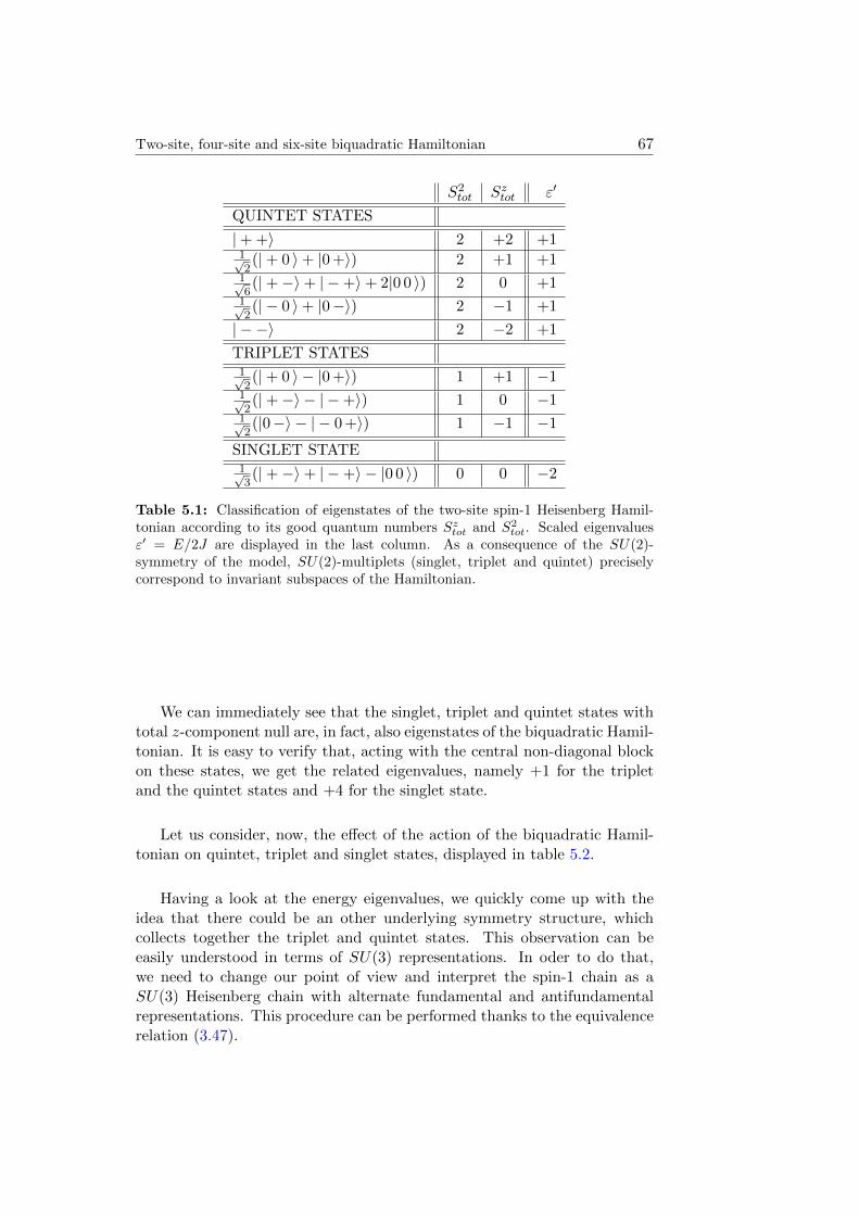
Two-site, four-site and six-site biquadratic Hamiltonian 67
S2tot Sztot ε′
QUINTET STATES
|+ +〉 2 +2 +11√2(|+ 0 〉+ |0 +〉) 2 +1 +1
1√6(|+−〉+ | −+〉+ 2|0 0 〉) 2 0 +1
1√2(| − 0 〉+ |0−〉) 2 −1 +1
| − −〉 2 −2 +1
TRIPLET STATES1√2(|+ 0 〉 − |0 +〉) 1 +1 −1
1√2(|+−〉 − | −+〉) 1 0 −1
1√2(|0−〉 − | − 0 +〉) 1 −1 −1
SINGLET STATE1√3(|+−〉+ | −+〉 − |0 0 〉) 0 0 −2
Table 5.1: Classification of eigenstates of the two-site spin-1 Heisenberg Hamil-tonian according to its good quantum numbers Sztot and S2
tot. Scaled eigenvaluesε′ = E/2J are displayed in the last column. As a consequence of the SU(2)-symmetry of the model, SU(2)-multiplets (singlet, triplet and quintet) preciselycorrespond to invariant subspaces of the Hamiltonian.
We can immediately see that the singlet, triplet and quintet states withtotal z-component null are, in fact, also eigenstates of the biquadratic Hamil-tonian. It is easy to verify that, acting with the central non-diagonal blockon these states, we get the related eigenvalues, namely +1 for the tripletand the quintet states and +4 for the singlet state.
Let us consider, now, the effect of the action of the biquadratic Hamil-tonian on quintet, triplet and singlet states, displayed in table 5.2.
Having a look at the energy eigenvalues, we quickly come up with theidea that there could be an other underlying symmetry structure, whichcollects together the triplet and quintet states. This observation can beeasily understood in terms of SU(3) representations. In oder to do that,we need to change our point of view and interpret the spin-1 chain as aSU(3) Heisenberg chain with alternate fundamental and antifundamentalrepresentations. This procedure can be performed thanks to the equivalencerelation (3.47).
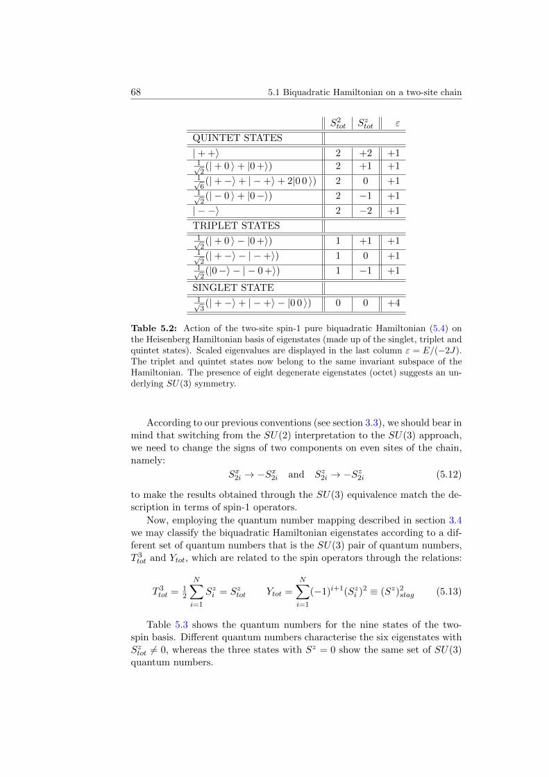
68 5.1 Biquadratic Hamiltonian on a two-site chain
S2tot Sztot ε
QUINTET STATES
|+ +〉 2 +2 +11√2(|+ 0 〉+ |0 +〉) 2 +1 +1
1√6(|+−〉+ | −+〉+ 2|0 0 〉) 2 0 +1
1√2(| − 0 〉+ |0−〉) 2 −1 +1
| − −〉 2 −2 +1
TRIPLET STATES1√2(|+ 0 〉 − |0 +〉) 1 +1 +1
1√2(|+−〉 − | −+〉) 1 0 +1
1√2(|0−〉 − | − 0 +〉) 1 −1 +1
SINGLET STATE1√3(|+−〉+ | −+〉 − |0 0 〉) 0 0 +4
Table 5.2: Action of the two-site spin-1 pure biquadratic Hamiltonian (5.4) onthe Heisenberg Hamiltonian basis of eigenstates (made up of the singlet, triplet andquintet states). Scaled eigenvalues are displayed in the last column ε = E/(−2J).The triplet and quintet states now belong to the same invariant subspace of theHamiltonian. The presence of eight degenerate eigenstates (octet) suggests an un-derlying SU(3) symmetry.
According to our previous conventions (see section 3.3), we should bear inmind that switching from the SU(2) interpretation to the SU(3) approach,we need to change the signs of two components on even sites of the chain,namely:
Sx2i → −Sx2i and Sz2i → −Sz2i (5.12)
to make the results obtained through the SU(3) equivalence match the de-scription in terms of spin-1 operators.
Now, employing the quantum number mapping described in section 3.4we may classify the biquadratic Hamiltonian eigenstates according to a dif-ferent set of quantum numbers that is the SU(3) pair of quantum numbers,T 3tot and Ytot, which are related to the spin operators through the relations:
T 3tot = 1
2
N∑i=1
Szi = Sztot Ytot =N∑i=1
(−1)i+1(Szi )2 ≡ (Sz)2stag (5.13)
Table 5.3 shows the quantum numbers for the nine states of the two-spin basis. Different quantum numbers characterise the six eigenstates withSztot 6= 0, whereas the three states with Sz = 0 show the same set of SU(3)quantum numbers.
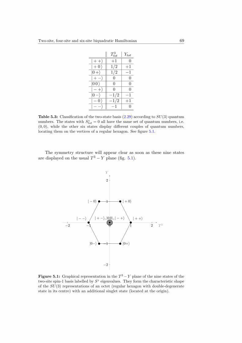
Two-site, four-site and six-site biquadratic Hamiltonian 69
T 3tot Ytot
|+ +〉 +1 0
|+ 0 〉 1/2 +1
|0 +〉 1/2 −1
|+−〉 0 0
|0 0 〉 0 0
| −+〉 0 0
|0−〉 −1/2 −1
| − 0 〉 −1/2 +1
| − −〉 −1 0
Table 5.3: Classification of the two-state basis (2.29) according to SU(3) quantumnumbers. The states with Sztot = 0 all have the same set of quantum numbers, i.e.(0, 0), while the other six states display different couples of quantum numbers,locating them on the vertices of a regular hexagon. See figure 5.1.
The symmetry structure will appear clear as soon as these nine statesare displayed on the usual T 3 − Y plane (fig. 5.1).
T 3
Y
21012
2
1
1
2
| + +i
| + 0i| 0i
| i
|0i |0+i
| + i, |0 0i, | +i
1
Figure 5.1: Graphical representation in the T 3−Y plane of the nine states of thetwo-site spin-1 basis labelled by Sz eigenvalues. They form the characteristic shapeof the SU(3) representations of an octet (regular hexagon with double-degeneratestate in its centre) with an additional singlet state (located at the origin).
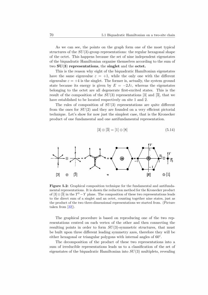
70 5.1 Biquadratic Hamiltonian on a two-site chain
As we can see, the points on the graph form one of the most typicalstructures of the SU(3)-group representations: the regular hexagonal shapeof the octet. This happens because the set of nine independent eigenstatesof the biquadratic Hamiltonian organise themselves according to the sum oftwo SU(3) representations, the singlet and the octet.
This is the reason why eight of the biquadratic Hamiltonian eigenstateshave the same eigenvalue ε = +1, while the only one with the differenteigenvalue ε = +4 is the singlet. The former is, actually, the system groundstate because its energy is given by E = −2Jε, whereas the eigenstatesbelonging to the octet are all degenerate first-excited states. This is theresult of the composition of the SU(3) representations [3] and [3], that wehave established to be located respectively on site 1 and 2.
The rules of composition of SU(3) representations are quite differentfrom the ones for SU(2) and they are founded on a very efficient pictorialtechnique. Let’s show for now just the simplest case, that is the Kroneckerproduct of one fundamental and one antifundamental representation.
[3]⊗ [3] = [1]⊕ [8] (5.14)
Figure 5.2: Graphical composition technique for the fundamental and antifunda-mental representations. It is shown the reduction method for the Kronecker productof [3]⊗ [3] in the T 3−Y plane. The composition of these two representations leadsto the direct sum of a singlet and an octet, counting together nine states, just asthe product of the two three-dimensional representations we started from. (Picturetaken from [22]).
The graphical procedure is based on reproducing one of the two rep-resentations centred on each vertex of the other and then connecting theresulting points in order to form SU(3)-symmetric structures, that mustbe built upon three different leading symmetry axes, therefore they will beeither hexagonal or triangular polygons with internal angles of 60.
The decomposition of the product of these two representations into asum of irreducible representations leads us to a classification of the set ofeigenstates of the biquadratic Hamiltonian into SU(3) multiplets, revealing
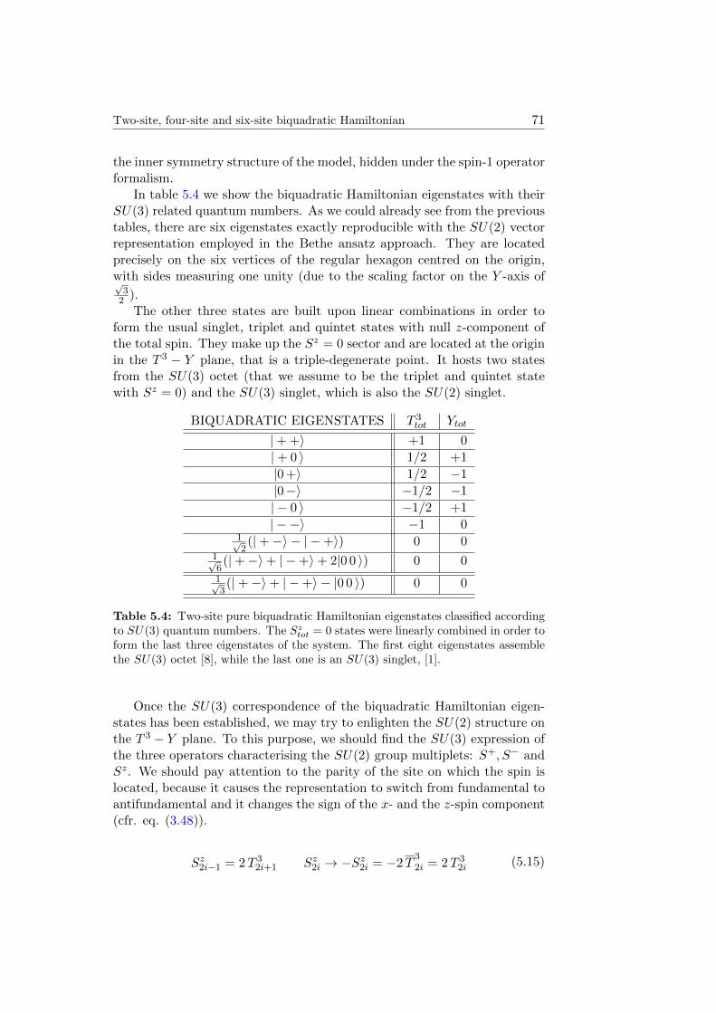
Two-site, four-site and six-site biquadratic Hamiltonian 71
the inner symmetry structure of the model, hidden under the spin-1 operatorformalism.
In table 5.4 we show the biquadratic Hamiltonian eigenstates with theirSU(3) related quantum numbers. As we could already see from the previoustables, there are six eigenstates exactly reproducible with the SU(2) vectorrepresentation employed in the Bethe ansatz approach. They are locatedprecisely on the six vertices of the regular hexagon centred on the origin,with sides measuring one unity (due to the scaling factor on the Y -axis of√
32 ).
The other three states are built upon linear combinations in order toform the usual singlet, triplet and quintet states with null z-component ofthe total spin. They make up the Sz = 0 sector and are located at the originin the T 3 − Y plane, that is a triple-degenerate point. It hosts two statesfrom the SU(3) octet (that we assume to be the triplet and quintet statewith Sz = 0) and the SU(3) singlet, which is also the SU(2) singlet.
BIQUADRATIC EIGENSTATES T 3tot Ytot
|+ +〉 +1 0
|+ 0 〉 1/2 +1
|0 +〉 1/2 −1
|0−〉 −1/2 −1
| − 0 〉 −1/2 +1
| − −〉 −1 01√2(|+−〉 − | −+〉) 0 0
1√6(|+−〉+ | −+〉+ 2|0 0 〉) 0 0
1√3(|+−〉+ | −+〉 − |0 0 〉) 0 0
Table 5.4: Two-site pure biquadratic Hamiltonian eigenstates classified accordingto SU(3) quantum numbers. The Sztot = 0 states were linearly combined in order toform the last three eigenstates of the system. The first eight eigenstates assemblethe SU(3) octet [8], while the last one is an SU(3) singlet, [1].
Once the SU(3) correspondence of the biquadratic Hamiltonian eigen-states has been established, we may try to enlighten the SU(2) structure onthe T 3 − Y plane. To this purpose, we should find the SU(3) expression ofthe three operators characterising the SU(2) group multiplets: S+, S− andSz. We should pay attention to the parity of the site on which the spin islocated, because it causes the representation to switch from fundamental toantifundamental and it changes the sign of the x- and the z-spin component(cfr. eq. (3.48)).
Sz2i−1 = 2T 32i+1 Sz2i → −Sz2i = −2T
32i = 2T 3
2i (5.15)
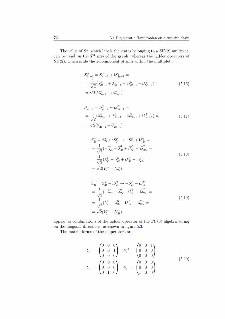
72 5.1 Biquadratic Hamiltonian on a two-site chain
The value of Sz, which labels the states belonging to a SU(2) multiplet,can be read on the T 3 axis of the graph, whereas the ladder operators ofSU(2), which scale the z-component of spin within the multiplet:
S+2i−1 = Sx2i−1 + iSy2i−1 =
=1√2
(λ42i−1 + λ62i−1 + iλ52i−1 − iλ72i−1) =
=√
2(V −2i−1 + U+2i−1)
(5.16)
S−2i−1 = Sx2i−1 − iSy2i−1 =
=1√2
(λ42i−1 + λ62i−1 − iλ52i−1 + iλ72i−1) =
=√
2(V −2i−1 + U+2i−1)
(5.17)
S+2i = Sx2i + iSy2i → −Sx2i + iSy2i =
=1√2
(−λ42i − λ62i + iλ
52i − iλ
72i) =
=1√2
(λ42i + λ62i + iλ52i − iλ72i) =
=√
2(V +2i + U−2i)
(5.18)
S−2i = Sx2i − iSy2i → −Sx2i − iSy2i =
=1√2
(−λ42i − λ62i − iλ
52i + iλ
72i) =
=1√2
(λ42i + λ62i − iλ52i + iλ72i) =
=√
2(V −2i + U+2i)
(5.19)
appear as combinations of the ladder operator of the SU(3) algebra actingon the diagonal directions, as shown in figure 5.3.
The matrix forms of these operators are:
U+i =
0 0 00 0 10 0 0
V +i =
0 0 10 0 00 0 0
U−i =
0 0 00 0 00 1 0
V −i =
0 0 00 0 01 0 0
(5.20)
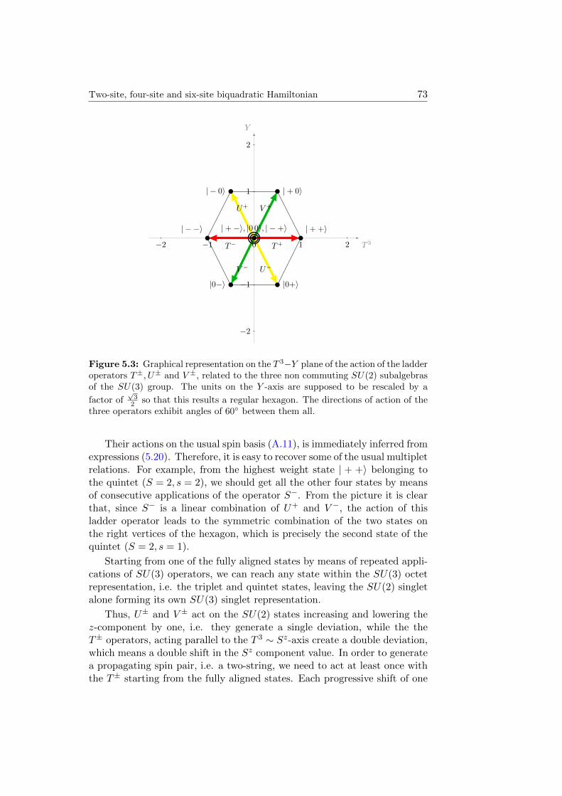
Two-site, four-site and six-site biquadratic Hamiltonian 73
T 3
Y
21012
2
1
1
2
T+T
V +
V
U+
U
| + +i
| + 0i| 0i
| i
|0i |0+i
| + i, |0 0i, | +i
1
Figure 5.3: Graphical representation on the T 3−Y plane of the action of the ladderoperators T±, U± and V ±, related to the three non commuting SU(2) subalgebrasof the SU(3) group. The units on the Y -axis are supposed to be rescaled by a
factor of√32 so that this results a regular hexagon. The directions of action of the
three operators exhibit angles of 60 between them all.
Their actions on the usual spin basis (A.11), is immediately inferred fromexpressions (5.20). Therefore, it is easy to recover some of the usual multipletrelations. For example, from the highest weight state | + +〉 belonging tothe quintet (S = 2, s = 2), we should get all the other four states by meansof consecutive applications of the operator S−. From the picture it is clearthat, since S− is a linear combination of U+ and V −, the action of thisladder operator leads to the symmetric combination of the two states onthe right vertices of the hexagon, which is precisely the second state of thequintet (S = 2, s = 1).
Starting from one of the fully aligned states by means of repeated appli-cations of SU(3) operators, we can reach any state within the SU(3) octetrepresentation, i.e. the triplet and quintet states, leaving the SU(2) singletalone forming its own SU(3) singlet representation.
Thus, U± and V ± act on the SU(2) states increasing and lowering thez-component by one, i.e. they generate a single deviation, while the theT± operators, acting parallel to the T 3 ∼ Sz-axis create a double deviation,which means a double shift in the Sz component value. In order to generatea propagating spin pair, i.e. a two-string, we need to act at least once withthe T± starting from the fully aligned states. Each progressive shift of one
74 5.1 Biquadratic Hamiltonian on a two-site chain
unity towards the origin of the plane represents the creation of one furtherpropagating couple, which cannot be identified in general because it is usu-ally defined as a linear combination which has to satisfy the Hamiltonianeigenvalue equation.
Although this is the simplest case of biquadratic Hamiltonian, theselatest considerations still hold even for a longer chain, with arbitrary buteven number of sites.
In order to get a confirmation of the technique employed, we may try thenumerical approach with the SU(3) Hamiltonian. This will be useful lateron, when we will deal with a larger number of sites for which the standardHamiltonian operator representation is (3N × 3N )-dimensional.
Focusing right now on the N = 2 site case, the Hamiltonian which weare going to study is the (3.48):
HF⊗A(J) = J
8∑α=1
[λα1 λ
α2 + λ
α2 λ
α1
](5.21)
where we assumed periodic boundary conditions as usual.
Evaluating this operator with the assistance of Mathematica, that pro-vides us with the complete set of eigenstates and eigenvalues of the model,we can see (table 5.6) that the eigenvectors appear in the shape of nine-dimensional vectors, with coefficients representing the decomposition on thecanonical C9 basis. These nine basis states can be built as the Kroneckerproduct of the three-dimensional vectors corresponding to the states of thetwo spin variables located on the two sites. Working in the SU(3) frameworkwe can use the single-site basis states (B.30), (B.31) and (B.32). The two-site joint basis will be the tensor product, organised in a nine-dimensionalvector displaying the conventional ordering:
|u〉|d〉|s〉
⊗|u〉|d〉|s〉
=
|uu〉|ud〉|us〉|du〉|dd〉|ds〉|su〉|sd〉|ss〉
(5.22)
In order to recover the interpretation in terms of spin-1 variables, we mustrelate the two-spin basis states to the nine canonical basis vectors for theHilbert space on which the SU(3) Hamiltonian acts. The correspondenceshould be based on the single spin basis (A.11), recalling that the order ofSz eigenstates is slightly different that the usual one (2.29), leading to the
Two-site, four-site and six-site biquadratic Hamiltonian 75
nine-dimensional basis vector, which should be decomposed according to thefollowing ordering:
|+〉|−〉| 0 〉
⊗|+〉|−〉| 0 〉
=
|+ +〉|+−〉|+ 0〉| −+〉| − −〉| − 0〉|0 +〉|0−〉| 0 0〉
(5.23)
While looking for the correspondence between the SU(3) canonical basis(5.22) and the spin-1 basis built on Sz eigenstates, we should pay particularattention to even sites. In fact, in order to establish the equivalence of theSU(3) Heisenberg chain with the pure-biquadratic spin-1 model, the signsof the two spin operators Sz and Sx on even sites have been altered.
Therefore, we should find an unitary operator U , that accomplishes thispurpose, namely:
U †Sx2iU = −Sx2i U †Sy2iU = Sy2i U †Sz2iU = −Sz2i (5.24)
Writing down the most general 3 × 3 matrix and imposing the constraintsgiven by the three former definitions of the action of the transformation Uon spin operators, we get the following matrix form:
U =
0 1 01 0 00 0 −1
(5.25)
which acts on a one-spin basis (|+〉, |−〉, |0〉) of an even site exchangingthe roles of the Sz = ±1 eigenstates and adding a minus to the Sz = 0eigenstate. We notice that the inverse of this matrix U−1 = U † is equalto U itself. The global transformation operator acting on a couple of twoneighbouring spins is given by the Kronecker product I ⊗ U , because thetransformation (5.24) should be performed only on the even sites.
I⊗ U =
0 1 01 0 00 0 −1
0 1 01 0 00 0 −1
0 1 01 0 00 0 −1
(5.26)
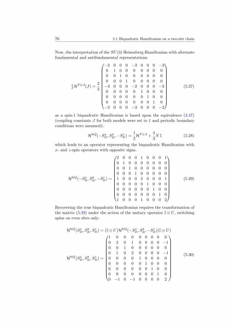
76 5.1 Biquadratic Hamiltonian on a two-site chain
Now, the interpretation of the SU(3) Heisenberg Hamiltonian with alternatefundamental and antifundamental representations
1JHF⊗A(J) =
2
3
−2 0 0 0 −3 0 0 0 −30 1 0 0 0 0 0 0 00 0 1 0 0 0 0 0 00 0 0 1 0 0 0 0 0−3 0 0 0 −2 0 0 0 −30 0 0 0 0 1 0 0 00 0 0 0 0 0 1 0 00 0 0 0 0 0 0 1 0−3 0 0 0 −3 0 0 0 −2
(5.27)
as a spin-1 biquadratic Hamiltonian is based upon the equivalence (3.47)(coupling constants J for both models were set to 1 and periodic boundaryconditions were assumed):
HbiQ(−Sx2i, Sy2i,−Sz2i) =1
2HF⊗A +
4
3N I (5.28)
which leads to an operator representing the biquadratic Hamiltonian withx- and z-spin operators with opposite signs.
HbiQ(−Sx2i, Sy2i,−Sz2i) =
2 0 0 0 1 0 0 0 10 1 0 0 0 0 0 0 00 0 1 0 0 0 0 0 00 0 0 1 0 0 0 0 01 0 0 0 2 0 0 0 10 0 0 0 0 1 0 0 00 0 0 0 0 0 1 0 00 0 0 0 0 0 0 1 01 0 0 0 1 0 0 0 2
(5.29)
Recovering the true biquadratic Hamiltonian requires the transformation ofthe matrix (5.29) under the action of the unitary operator I⊗ U , switchingspins on even sites only.
HbiQ(Sx2i, Sy2i, S
z2i) = (I⊗ U)HbiQ(−Sx2i, Sy2i,−Sz2i)(I⊗ U)
HbiQ(Sx2i, Sy2i, S
z2i) =
1 0 0 0 0 0 0 0 00 2 0 1 0 0 0 0 −10 0 1 0 0 0 0 0 00 1 0 2 0 0 0 0 −10 0 0 0 1 0 0 0 00 0 0 0 0 1 0 0 00 0 0 0 0 0 1 0 00 0 0 0 0 0 0 1 00 −1 0 −1 0 0 0 0 2
(5.30)
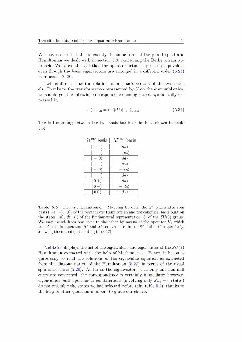
Two-site, four-site and six-site biquadratic Hamiltonian 77
We may notice that this is exactly the same form of the pure biquadraticHamiltonian we dealt with in section 2.3, concerning the Bethe ansatz ap-proach. We stress the fact that the operator action is perfectly equivalenteven though the basis eigenvectors are arranged in a different order (5.23)from usual (2.29).
Let us discuss now the relation among basis vectors of the two mod-els. Thanks to the transformation represented by U on the even sublattice,we should get the following correspondence among states, symbolically ex-pressed by:
| , 〉+,−,0 = (I⊗ U)| , 〉u,d,s (5.31)
The full mapping between the two basis has been built as shown in table5.5:
HbiQ basis HF⊗A basis
|+ +〉 |ud〉|+−〉 −|us〉|+ 0〉 |sd〉| −+〉 |uu〉| − 0〉 −|ss〉| − −〉 |dd〉| 0 +〉 |su〉| 0−〉 −|ds〉| 0 0 〉 |du〉
Table 5.5: Two site Hamiltonian. Mapping between the Sz eigenstates spinbasis (|+〉, |−〉, | 0 〉) of the biquadratic Hamiltonian and the canonical basis built onthe states (|u〉, |d〉, |s〉) of the fundamental representation [3] of the SU(3) group.We may switch from one basis to the other by means of the operator U , whichtransforms the operators Sx and Sz on even sites into −Sx and −Sz respectively,allowing the mapping according to (3.47).
Table 5.6 displays the list of the eigenvalues and eigenstates of the SU(3)Hamiltonian extracted with the help of Mathematica. Hence, it becomesquite easy to read the solutions of the eigenvalue equation as extractedfrom the diagonalisation of the Hamiltonian (5.27) in terms of the usualspin state basis (2.29). As far as the eigenvectors with only one non-nullentry are concerned, the correspondence is certainly immediate; however,eigenvalues built upon linear combinations (involving only Sztot = 0 states)do not resemble the states we had selected before (cfr. table 5.2), thanks tothe help of other quantum numbers to guide our choice.
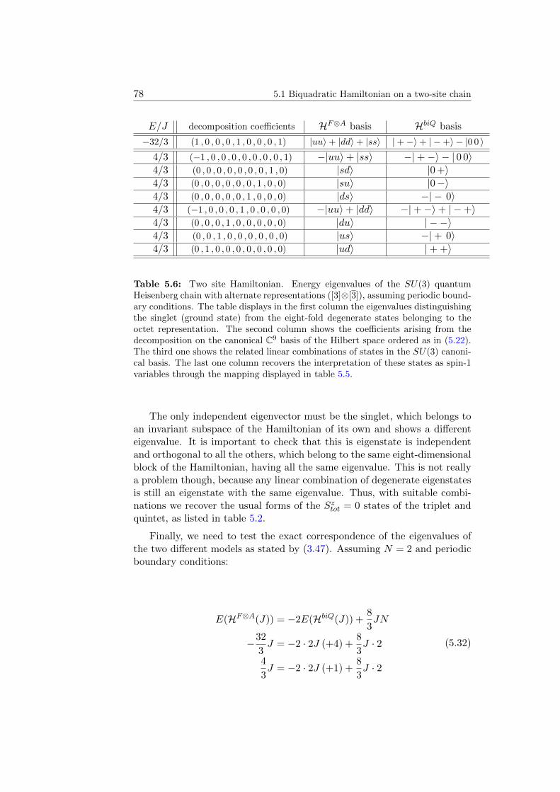
78 5.1 Biquadratic Hamiltonian on a two-site chain
E/J decomposition coefficients HF⊗A basis HbiQ basis
−32/3 (1 , 0 , 0 , 0 , 1 , 0 , 0 , 0 , 1) |uu〉+ |dd〉+ |ss〉 |+−〉+ | −+〉 − |0 0 〉4/3 (−1 , 0 , 0 , 0 , 0 , 0 , 0 , 0 , 1) −|uu〉+ |ss〉 −|+−〉 − | 0 0〉4/3 (0 , 0 , 0 , 0 , 0 , 0 , 0 , 1 , 0) |sd〉 |0 +〉4/3 (0 , 0 , 0 , 0 , 0 , 0 , 1 , 0 , 0) |su〉 |0−〉4/3 (0 , 0 , 0 , 0 , 0 , 1 , 0 , 0 , 0) |ds〉 −| − 0〉4/3 (−1 , 0 , 0 , 0 , 1 , 0 , 0 , 0 , 0) −|uu〉+ |dd〉 −|+−〉+ | −+〉4/3 (0 , 0 , 0 , 1 , 0 , 0 , 0 , 0 , 0) |du〉 | − −〉4/3 (0 , 0 , 1 , 0 , 0 , 0 , 0 , 0 , 0) |us〉 −|+ 0〉4/3 (0 , 1 , 0 , 0 , 0 , 0 , 0 , 0 , 0) |ud〉 |+ +〉
Table 5.6: Two site Hamiltonian. Energy eigenvalues of the SU(3) quantumHeisenberg chain with alternate representations ([3]⊗[3]), assuming periodic bound-ary conditions. The table displays in the first column the eigenvalues distinguishingthe singlet (ground state) from the eight-fold degenerate states belonging to theoctet representation. The second column shows the coefficients arising from thedecomposition on the canonical C9 basis of the Hilbert space ordered as in (5.22).The third one shows the related linear combinations of states in the SU(3) canoni-cal basis. The last one column recovers the interpretation of these states as spin-1variables through the mapping displayed in table 5.5.
The only independent eigenvector must be the singlet, which belongs toan invariant subspace of the Hamiltonian of its own and shows a differenteigenvalue. It is important to check that this is eigenstate is independentand orthogonal to all the others, which belong to the same eight-dimensionalblock of the Hamiltonian, having all the same eigenvalue. This is not reallya problem though, because any linear combination of degenerate eigenstatesis still an eigenstate with the same eigenvalue. Thus, with suitable combi-nations we recover the usual forms of the Sztot = 0 states of the triplet andquintet, as listed in table 5.2.
Finally, we need to test the exact correspondence of the eigenvalues ofthe two different models as stated by (3.47). Assuming N = 2 and periodicboundary conditions:
E(HF⊗A(J)) = −2E(HbiQ(J)) +8
3JN
−32
3J = −2 · 2J (+4) +
8
3J · 2
4
3J = −2 · 2J (+1) +
8
3J · 2
(5.32)
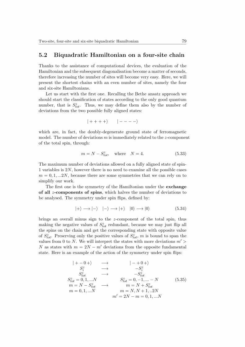
Two-site, four-site and six-site biquadratic Hamiltonian 79
5.2 Biquadratic Hamiltonian on a four-site chain
Thanks to the assistance of computational devices, the evaluation of theHamiltonian and the subsequent diagonalisation become a matter of seconds,therefore increasing the number of sites will become very easy. Here, we willpresent the shortest chains with an even number of sites, namely the fourand six-site Hamiltonians.
Let us start with the first one. Recalling the Bethe ansatz approach weshould start the classification of states according to the only good quantumnumber, that is Sztot. Thus, we may define them also by the number ofdeviations from the two possible fully aligned states:
|+ + + +〉 | − − −−〉
which are, in fact, the doubly-degenerate ground state of ferromagneticmodel. The number of deviationsm is immediately related to the z-componentof the total spin, through:
m = N − Sztot, where N = 4. (5.33)
The maximum number of deviations allowed on a fully aligned state of spin-1 variables is 2N , however there is no need to examine all the possible casesm = 0, 1, ...2N , because there are some symmetries that we can rely on tosimplify our work.
The first one is the symmetry of the Hamiltonian under the exchangeof all z-components of spins, which halves the number of deviations tobe analysed. The symmetry under spin flips, defined by:
|+〉 −→ |−〉 |−〉 −→ |+〉 |0〉 −→ |0〉 (5.34)
brings an overall minus sign to the z-component of the total spin, thusmaking the negative values of Sztot redundant, because we may just flip allthe spins on the chain and get the corresponding state with opposite valueof Sztot. Preserving only the positive values of Sztot, m is bound to span thevalues from 0 to N . We will interpret the states with more deviations m′ >N as states with m = 2N −m′ deviations from the opposite fundamentalstate. Here is an example of the action of the symmetry under spin flips:
|+− 0 +〉 −→ | −+ 0 +〉Szi −→ −SziSztot −→ −Sztot
Sztot = 0, 1, ...N Sztot = 0,−1, ...−Nm = N − Sztot −→ m = N + Sztotm = 0, 1, ...N m = N,N + 1, ..2N
m′ = 2N −m = 0, 1, ...N
(5.35)
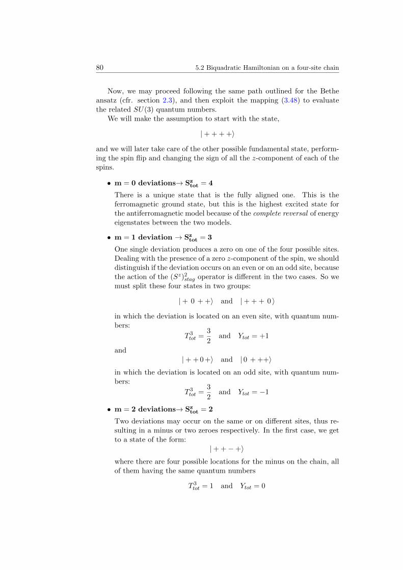
80 5.2 Biquadratic Hamiltonian on a four-site chain
Now, we may proceed following the same path outlined for the Betheansatz (cfr. section 2.3), and then exploit the mapping (3.48) to evaluatethe related SU(3) quantum numbers.
We will make the assumption to start with the state,
|+ + + +〉
and we will later take care of the other possible fundamental state, perform-ing the spin flip and changing the sign of all the z-component of each of thespins.
• m = 0 deviations→ Sztot = 4
There is a unique state that is the fully aligned one. This is theferromagnetic ground state, but this is the highest excited state forthe antiferromagnetic model because of the complete reversal of energyeigenstates between the two models.
• m = 1 deviation → Sztot = 3
One single deviation produces a zero on one of the four possible sites.Dealing with the presence of a zero z-component of the spin, we shoulddistinguish if the deviation occurs on an even or on an odd site, becausethe action of the (Sz)2stag operator is different in the two cases. So wemust split these four states in two groups:
|+ 0 + +〉 and |+ + + 0 〉
in which the deviation is located on an even site, with quantum num-bers:
T 3tot =
3
2and Ytot = +1
and|+ + 0 +〉 and | 0 + ++〉
in which the deviation is located on an odd site, with quantum num-bers:
T 3tot =
3
2and Ytot = −1
• m = 2 deviations→ Sztot = 2
Two deviations may occur on the same or on different sites, thus re-sulting in a minus or two zeroes respectively. In the first case, we getto a state of the form:
|+ +−+〉where there are four possible locations for the minus on the chain, allof them having the same quantum numbers
T 3tot = 1 and Ytot = 0
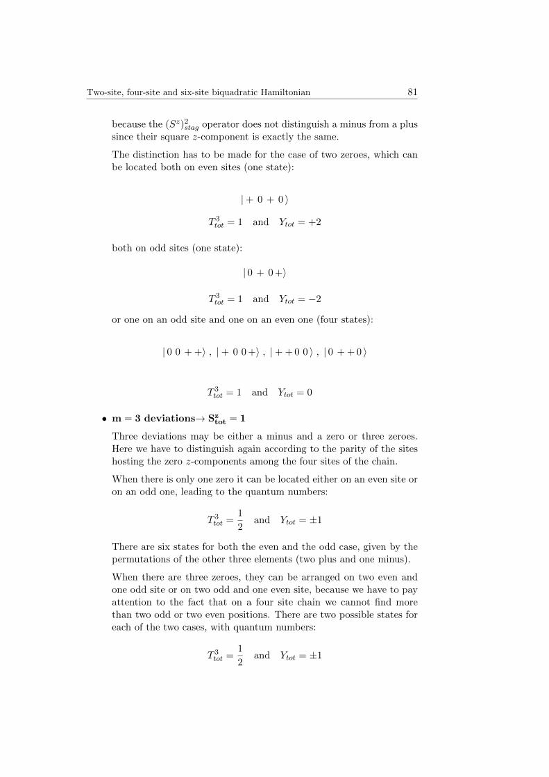
Two-site, four-site and six-site biquadratic Hamiltonian 81
because the (Sz)2stag operator does not distinguish a minus from a plussince their square z-component is exactly the same.
The distinction has to be made for the case of two zeroes, which canbe located both on even sites (one state):
|+ 0 + 0 〉
T 3tot = 1 and Ytot = +2
both on odd sites (one state):
| 0 + 0 +〉
T 3tot = 1 and Ytot = −2
or one on an odd site and one on an even one (four states):
| 0 0 + +〉 , |+ 0 0 +〉 , |+ + 0 0 〉 , | 0 + + 0 〉
T 3tot = 1 and Ytot = 0
• m = 3 deviations→ Sztot = 1
Three deviations may be either a minus and a zero or three zeroes.Here we have to distinguish again according to the parity of the siteshosting the zero z-components among the four sites of the chain.
When there is only one zero it can be located either on an even site oron an odd one, leading to the quantum numbers:
T 3tot =
1
2and Ytot = ±1
There are six states for both the even and the odd case, given by thepermutations of the other three elements (two plus and one minus).
When there are three zeroes, they can be arranged on two even andone odd site or on two odd and one even site, because we have to payattention to the fact that on a four site chain we cannot find morethan two odd or two even positions. There are two possible states foreach of the two cases, with quantum numbers:
T 3tot =
1
2and Ytot = ±1
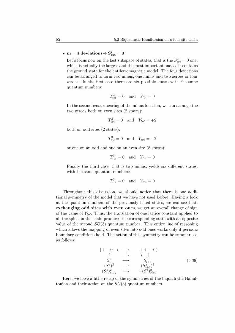
82 5.2 Biquadratic Hamiltonian on a four-site chain
• m = 4 deviations→ Sztot = 0
Let’s focus now on the last subspace of states, that is the Sztot = 0 one,which is actually the largest and the most important one, as it containsthe ground state for the antiferromagnetic model. The four deviationscan be arranged to form two minus, one minus and two zeroes or fourzeroes. In the first case there are six possible states with the samequantum numbers:
T 3tot = 0 and Ytot = 0
In the second case, uncaring of the minus location, we can arrange thetwo zeroes both on even sites (2 states):
T 3tot = 0 and Ytot = +2
both on odd sites (2 states):
T 3tot = 0 and Ytot = −2
or one on an odd and one on an even site (8 states):
T 3tot = 0 and Ytot = 0
Finally the third case, that is two minus, yields six different states,with the same quantum numbers:
T 3tot = 0 and Ytot = 0
Throughout this discussion, we should notice that there is one addi-tional symmetry of the model that we have not used before. Having a lookat the quantum numbers of the previously listed states, we can see that,exchanging odd sites with even ones, we get an overall change of signof the value of Ytot. Thus, the translation of one lattice constant applied toall the spins on the chain produces the corresponding state with an oppositevalue of the second SU(3) quantum number. This entire line of reasoningwhich allows the mapping of even sites into odd ones works only if periodicboundary conditions hold. The action of this symmetry can be summarisedas follows:
|+− 0 +〉 −→ |+ +− 0 〉i −→ i+ 1Szi −→ Szi+1
(Szi )2 −→ (Szi+1)2
(Sz)2stag −→ −(Sz)2stag
(5.36)
Here, we have a little recap of the symmetries of the biquadratic Hamil-tonian and their action on the SU(3) quantum numbers.
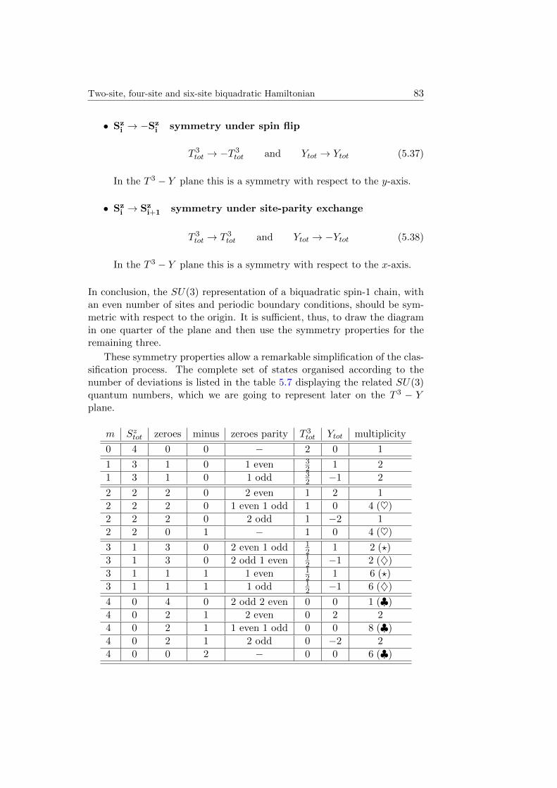
Two-site, four-site and six-site biquadratic Hamiltonian 83
• Szi → −Sz
i symmetry under spin flip
T 3tot → −T 3
tot and Ytot → Ytot (5.37)
In the T 3 − Y plane this is a symmetry with respect to the y-axis.
• Szi → Sz
i+1 symmetry under site-parity exchange
T 3tot → T 3
tot and Ytot → −Ytot (5.38)
In the T 3 − Y plane this is a symmetry with respect to the x-axis.
In conclusion, the SU(3) representation of a biquadratic spin-1 chain, withan even number of sites and periodic boundary conditions, should be sym-metric with respect to the origin. It is sufficient, thus, to draw the diagramin one quarter of the plane and then use the symmetry properties for theremaining three.
These symmetry properties allow a remarkable simplification of the clas-sification process. The complete set of states organised according to thenumber of deviations is listed in the table 5.7 displaying the related SU(3)quantum numbers, which we are going to represent later on the T 3 − Yplane.
m Sztot zeroes minus zeroes parity T 3tot Ytot multiplicity
0 4 0 0 − 2 0 1
1 3 1 0 1 even 32 1 2
1 3 1 0 1 odd 32 −1 2
2 2 2 0 2 even 1 2 1
2 2 2 0 1 even 1 odd 1 0 4 (♥)
2 2 2 0 2 odd 1 −2 1
2 2 0 1 − 1 0 4 (♥)
3 1 3 0 2 even 1 odd 12 1 2 (?)
3 1 3 0 2 odd 1 even 12 −1 2 (♦)
3 1 1 1 1 even 12 1 6 (?)
3 1 1 1 1 odd 12 −1 6 (♦)
4 0 4 0 2 odd 2 even 0 0 1 (♣)
4 0 2 1 2 even 0 2 2
4 0 2 1 1 even 1 odd 0 0 8 (♣)
4 0 2 1 2 odd 0 −2 2
4 0 0 2 − 0 0 6 (♣)
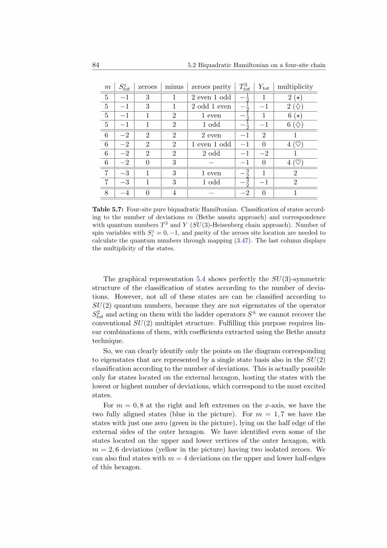
84 5.2 Biquadratic Hamiltonian on a four-site chain
m Sztot zeroes minus zeroes parity T 3tot Ytot multiplicity
5 −1 3 1 2 even 1 odd −12 1 2 (?)
5 −1 3 1 2 odd 1 even −12 −1 2 (♦)
5 −1 1 2 1 even −12 1 6 (?)
5 −1 1 2 1 odd −12 −1 6 (♦)
6 −2 2 2 2 even −1 2 1
6 −2 2 2 1 even 1 odd −1 0 4 (♥)
6 −2 2 2 2 odd −1 −2 1
6 −2 0 3 − −1 0 4 (♥)
7 −3 1 3 1 even −32 1 2
7 −3 1 3 1 odd −32 −1 2
8 −4 0 4 − −2 0 1
Table 5.7: Four-site pure biquadratic Hamiltonian. Classification of states accord-ing to the number of deviations m (Bethe ansatz approach) and correspondencewith quantum numbers T 3 and Y (SU(3)-Heisenberg chain approach). Number ofspin variables with Szi = 0,−1, and parity of the zeroes site location are needed tocalculate the quantum numbers through mapping (3.47). The last column displaysthe multiplicity of the states.
The graphical representation 5.4 shows perfectly the SU(3)-symmetricstructure of the classification of states according to the number of devia-tions. However, not all of these states are can be classified according toSU(2) quantum numbers, because they are not eigenstates of the operatorS2tot and acting on them with the ladder operators S± we cannot recover the
conventional SU(2) multiplet structure. Fulfilling this purpose requires lin-ear combinations of them, with coefficients extracted using the Bethe ansatztechnique.
So, we can clearly identify only the points on the diagram correspondingto eigenstates that are represented by a single state basis also in the SU(2)classification according to the number of deviations. This is actually possibleonly for states located on the external hexagon, hosting the states with thelowest or highest number of deviations, which correspond to the most excitedstates.
For m = 0, 8 at the right and left extremes on the x-axis, we have thetwo fully aligned states (blue in the picture). For m = 1, 7 we have thestates with just one zero (green in the picture), lying on the half edge of theexternal sides of the outer hexagon. We have identified even some of thestates located on the upper and lower vertices of the outer hexagon, withm = 2, 6 deviations (yellow in the picture) having two isolated zeroes. Wecan also find states with m = 4 deviations on the upper and lower half-edgesof this hexagon.
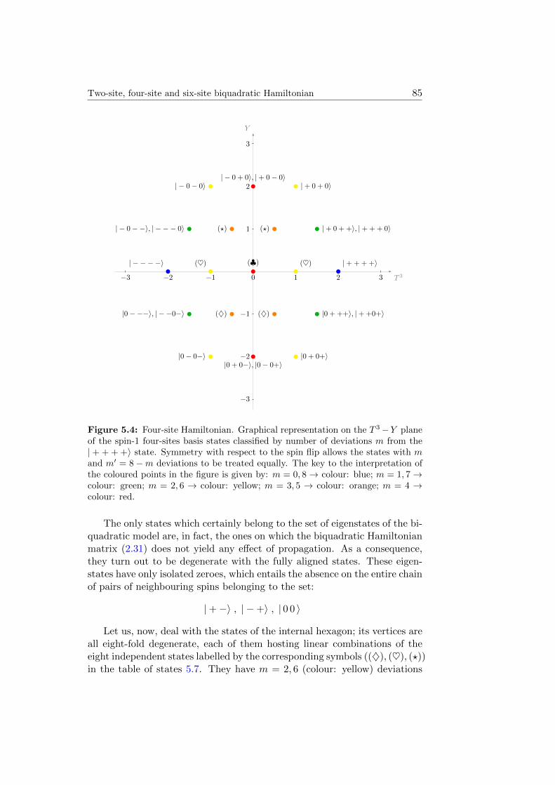
Two-site, four-site and six-site biquadratic Hamiltonian 85
T 3
Y
3210123
3
2
1
1
2
3
| + + + +i| i
| + 0 + +i, | + + + 0i| 0 i, | 0i
|0 i, | 0i |0 + ++i, | + +0+i
(~)
| + 0 + 0i| 0 0i
(~)
|0 0i |0 + 0+i
(?)
()
(?)
()
|0 + 0i, |0 0+i
| 0 + 0i, | + 0 0i
(|)
1
Figure 5.4: Four-site Hamiltonian. Graphical representation on the T 3−Y planeof the spin-1 four-sites basis states classified by number of deviations m from the|+ + + +〉 state. Symmetry with respect to the spin flip allows the states with mand m′ = 8−m deviations to be treated equally. The key to the interpretation ofthe coloured points in the figure is given by: m = 0, 8→ colour: blue; m = 1, 7→colour: green; m = 2, 6 → colour: yellow; m = 3, 5 → colour: orange; m = 4 →colour: red.
The only states which certainly belong to the set of eigenstates of the bi-quadratic model are, in fact, the ones on which the biquadratic Hamiltonianmatrix (2.31) does not yield any effect of propagation. As a consequence,they turn out to be degenerate with the fully aligned states. These eigen-states have only isolated zeroes, which entails the absence on the entire chainof pairs of neighbouring spins belonging to the set:
|+−〉 , | −+〉 , | 0 0 〉
Let us, now, deal with the states of the internal hexagon; its vertices areall eight-fold degenerate, each of them hosting linear combinations of theeight independent states labelled by the corresponding symbols ((♦), (♥), (?))in the table of states 5.7. They have m = 2, 6 (colour: yellow) deviations
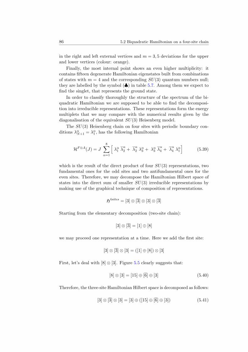
86 5.2 Biquadratic Hamiltonian on a four-site chain
in the right and left external vertices and m = 3, 5 deviations for the upperand lower vertices (colour: orange).
Finally, the most internal point shows an even higher multiplicity: itcontains fifteen degenerate Hamiltonian eigenstates built from combinationsof states with m = 4 and the corresponding SU(3) quantum numbers null;they are labelled by the symbol (♣) in table 5.7. Among them we expect tofind the singlet, that represents the ground state.
In order to classify thoroughly the structure of the spectrum of the bi-quadratic Hamiltonian we are supposed to be able to find the decomposi-tion into irreducible representations. These representations form the energymultiplets that we may compare with the numerical results given by thediagonalisation of the equivalent SU(3) Heisenberg model.
The SU(3) Heisenberg chain on four sites with periodic boundary con-ditions λαN+1 = λα1 , has the following Hamiltonian
HF⊗A(J) = J8∑
α=1
[λα1 λ
α2 + λ
α2 λ
α3 + λα3 λ
α4 + λ
α4 λ
α1
](5.39)
which is the result of the direct product of four SU(3) representations, twofundamental ones for the odd sites and two antifundamental ones for theeven sites. Therefore, we may decompose the Hamiltonian Hilbert space ofstates into the direct sum of smaller SU(3) irreducible representations bymaking use of the graphical technique of composition of representations.
H4sites = [3]⊗ [3]⊗ [3]⊗ [3]
Starting from the elementary decomposition (two-site chain):
[3]⊗ [3] = [1]⊕ [8]
we may proceed one representation at a time. Here we add the first site:
[3]⊗ [3]⊗ [3] = ([1]⊕ [8])⊗ [3]
First, let’s deal with [8]⊗ [3]. Figure 5.5 clearly suggests that:
[8]⊗ [3] = [15]⊕ [6]⊕ [3] (5.40)
Therefore, the three-site Hamiltonian Hilbert space is decomposed as follows:
[3]⊗ [3]⊗ [3] = [3]⊕ ([15]⊕ [6]⊕ [3]) (5.41)
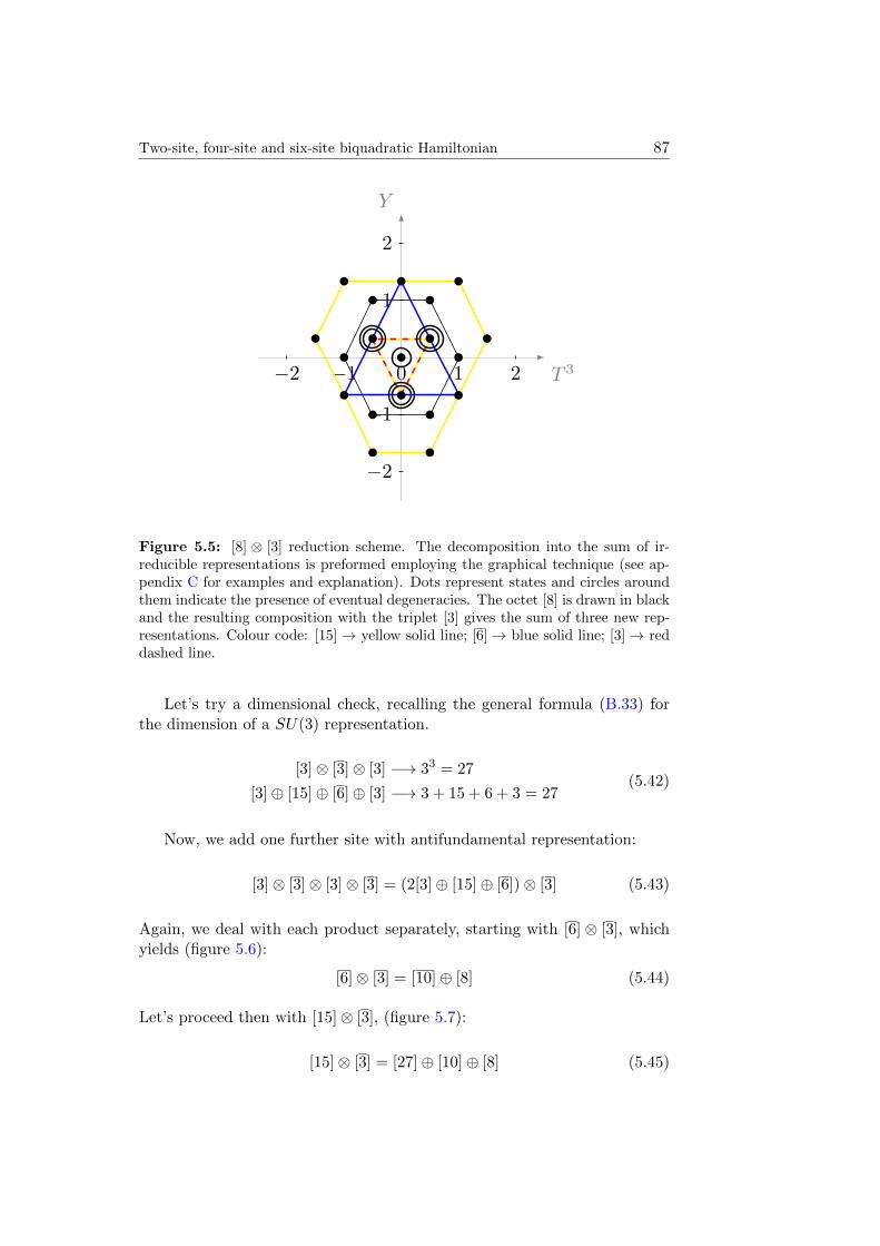
Two-site, four-site and six-site biquadratic Hamiltonian 87
T 3
Y
21012
2
1
1
2
1
Figure 5.5: [8] ⊗ [3] reduction scheme. The decomposition into the sum of ir-reducible representations is preformed employing the graphical technique (see ap-pendix C for examples and explanation). Dots represent states and circles aroundthem indicate the presence of eventual degeneracies. The octet [8] is drawn in blackand the resulting composition with the triplet [3] gives the sum of three new rep-resentations. Colour code: [15]→ yellow solid line; [6]→ blue solid line; [3]→ reddashed line.
Let’s try a dimensional check, recalling the general formula (B.33) forthe dimension of a SU(3) representation.
[3]⊗ [3]⊗ [3] −→ 33 = 27
[3]⊕ [15]⊕ [6]⊕ [3] −→ 3 + 15 + 6 + 3 = 27(5.42)
Now, we add one further site with antifundamental representation:
[3]⊗ [3]⊗ [3]⊗ [3] = (2[3]⊕ [15]⊕ [6])⊗ [3] (5.43)
Again, we deal with each product separately, starting with [6] ⊗ [3], whichyields (figure 5.6):
[6]⊗ [3] = [10]⊕ [8] (5.44)
Let’s proceed then with [15]⊗ [3], (figure 5.7):
[15]⊗ [3] = [27]⊕ [10]⊕ [8] (5.45)
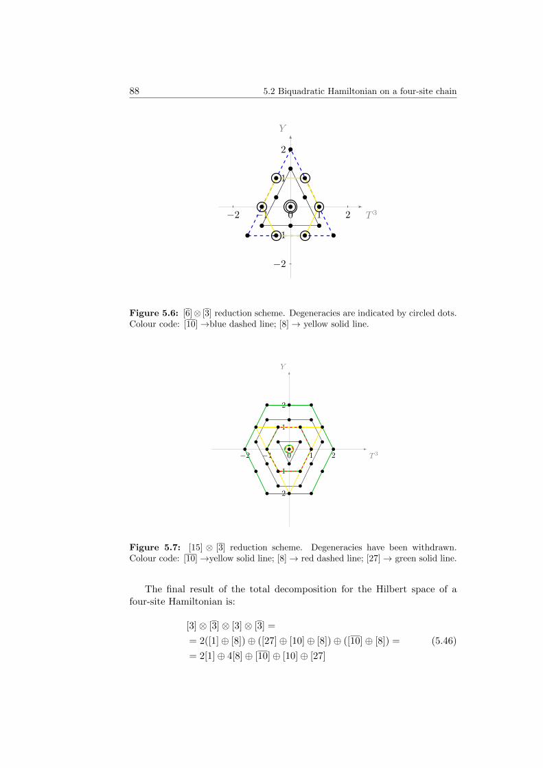
88 5.2 Biquadratic Hamiltonian on a four-site chain
T 3
Y
21012
2
1
1
2
1
Figure 5.6: [6]⊗ [3] reduction scheme. Degeneracies are indicated by circled dots.Colour code: [10]→blue dashed line; [8]→ yellow solid line.
T 3
Y
21012
2
1
1
2
1
Figure 5.7: [15] ⊗ [3] reduction scheme. Degeneracies have been withdrawn.Colour code: [10]→yellow solid line; [8]→ red dashed line; [27]→ green solid line.
The final result of the total decomposition for the Hilbert space of afour-site Hamiltonian is:
[3]⊗ [3]⊗ [3]⊗ [3] =
= 2([1]⊕ [8])⊕ ([27]⊕ [10]⊕ [8])⊕ ([10]⊕ [8]) =
= 2[1]⊕ 4[8]⊕ [10]⊕ [10]⊕ [27]
(5.46)
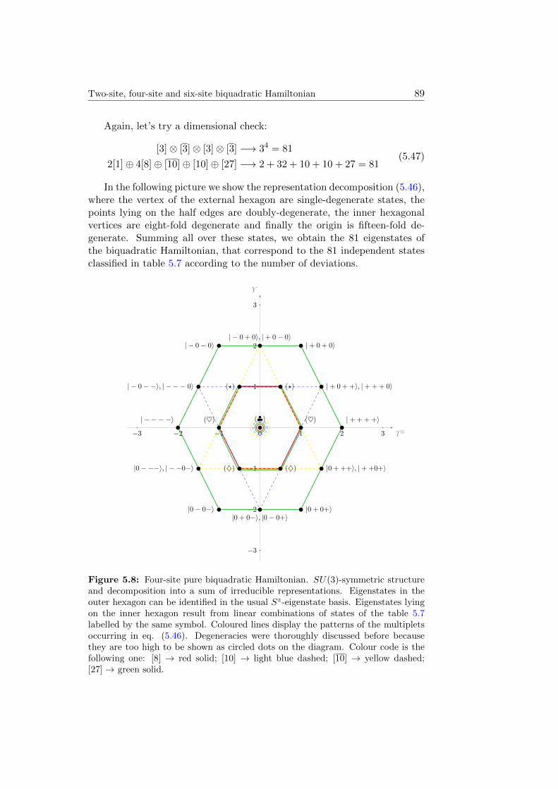
Two-site, four-site and six-site biquadratic Hamiltonian 89
Again, let’s try a dimensional check:
[3]⊗ [3]⊗ [3]⊗ [3] −→ 34 = 81
2[1]⊕ 4[8]⊕ [10]⊕ [10]⊕ [27] −→ 2 + 32 + 10 + 10 + 27 = 81(5.47)
In the following picture we show the representation decomposition (5.46),where the vertex of the external hexagon are single-degenerate states, thepoints lying on the half edges are doubly-degenerate, the inner hexagonalvertices are eight-fold degenerate and finally the origin is fifteen-fold de-generate. Summing all over these states, we obtain the 81 eigenstates ofthe biquadratic Hamiltonian, that correspond to the 81 independent statesclassified in table 5.7 according to the number of deviations.
T 3
Y
3210123
3
2
1
1
2
3
| + + + +i| i
| + 0 + +i, | + + + 0i| 0 i, | 0i
|0 i, | 0i |0 + ++i, | + +0+i
(~)
| + 0 + 0i| 0 0i
(~)
|0 0i |0 + 0+i
(?)
()
(?)
()
|0 + 0i, |0 0+i
| 0 + 0i, | + 0 0i
(|)
1
Figure 5.8: Four-site pure biquadratic Hamiltonian. SU(3)-symmetric structureand decomposition into a sum of irreducible representations. Eigenstates in theouter hexagon can be identified in the usual Sz-eigenstate basis. Eigenstates lyingon the inner hexagon result from linear combinations of states of the table 5.7labelled by the same symbol. Coloured lines display the patterns of the multipletsoccurring in eq. (5.46). Degeneracies were thoroughly discussed before becausethey are too high to be shown as circled dots on the diagram. Colour code is thefollowing one: [8] → red solid; [10] → light blue dashed; [10] → yellow dashed;[27]→ green solid.
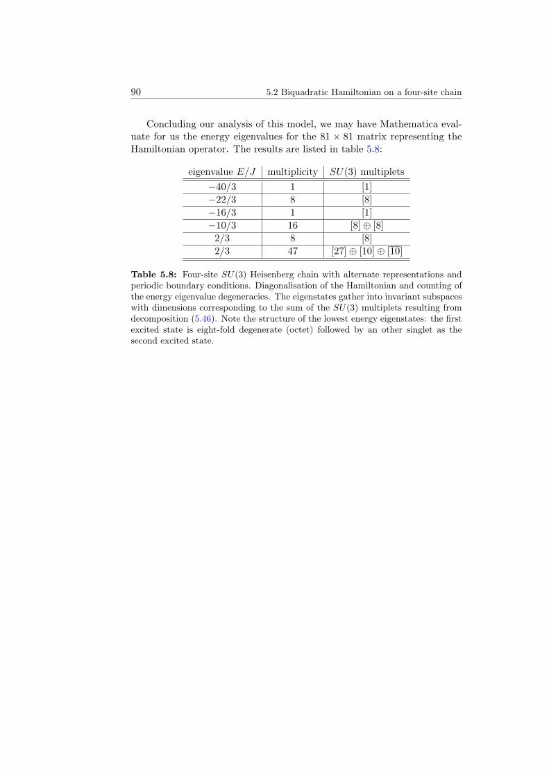
90 5.2 Biquadratic Hamiltonian on a four-site chain
Concluding our analysis of this model, we may have Mathematica eval-uate for us the energy eigenvalues for the 81 × 81 matrix representing theHamiltonian operator. The results are listed in table 5.8:
eigenvalue E/J multiplicity SU(3) multiplets
−40/3 1 [1]
−22/3 8 [8]
−16/3 1 [1]
−10/3 16 [8]⊕ [8]
2/3 8 [8]
2/3 47 [27]⊕ [10]⊕ [10]
Table 5.8: Four-site SU(3) Heisenberg chain with alternate representations andperiodic boundary conditions. Diagonalisation of the Hamiltonian and counting ofthe energy eigenvalue degeneracies. The eigenstates gather into invariant subspaceswith dimensions corresponding to the sum of the SU(3) multiplets resulting fromdecomposition (5.46). Note the structure of the lowest energy eigenstates: the firstexcited state is eight-fold degenerate (octet) followed by an other singlet as thesecond excited state.
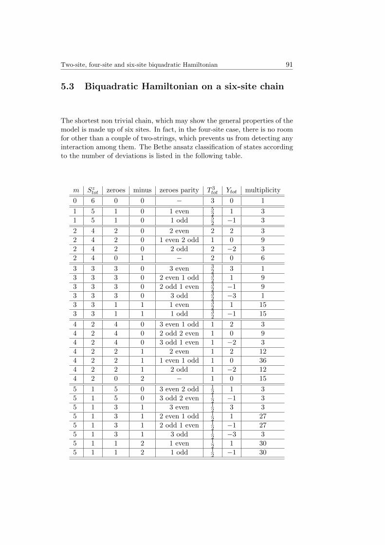
Two-site, four-site and six-site biquadratic Hamiltonian 91
5.3 Biquadratic Hamiltonian on a six-site chain
The shortest non trivial chain, which may show the general properties of themodel is made up of six sites. In fact, in the four-site case, there is no roomfor other than a couple of two-strings, which prevents us from detecting anyinteraction among them. The Bethe ansatz classification of states accordingto the number of deviations is listed in the following table.
m Sztot zeroes minus zeroes parity T 3tot Ytot multiplicity
0 6 0 0 − 3 0 1
1 5 1 0 1 even 52 1 3
1 5 1 0 1 odd 52 −1 3
2 4 2 0 2 even 2 2 3
2 4 2 0 1 even 2 odd 1 0 9
2 4 2 0 2 odd 2 −2 3
2 4 0 1 − 2 0 6
3 3 3 0 3 even 32 3 1
3 3 3 0 2 even 1 odd 32 1 9
3 3 3 0 2 odd 1 even 32 −1 9
3 3 3 0 3 odd 32 −3 1
3 3 1 1 1 even 32 1 15
3 3 1 1 1 odd 32 −1 15
4 2 4 0 3 even 1 odd 1 2 3
4 2 4 0 2 odd 2 even 1 0 9
4 2 4 0 3 odd 1 even 1 −2 3
4 2 2 1 2 even 1 2 12
4 2 2 1 1 even 1 odd 1 0 36
4 2 2 1 2 odd 1 −2 12
4 2 0 2 − 1 0 15
5 1 5 0 3 even 2 odd 12 1 3
5 1 5 0 3 odd 2 even 12 −1 3
5 1 3 1 3 even 12 3 3
5 1 3 1 2 even 1 odd 12 1 27
5 1 3 1 2 odd 1 even 12 −1 27
5 1 3 1 3 odd 12 −3 3
5 1 1 2 1 even 12 1 30
5 1 1 2 1 odd 12 −1 30
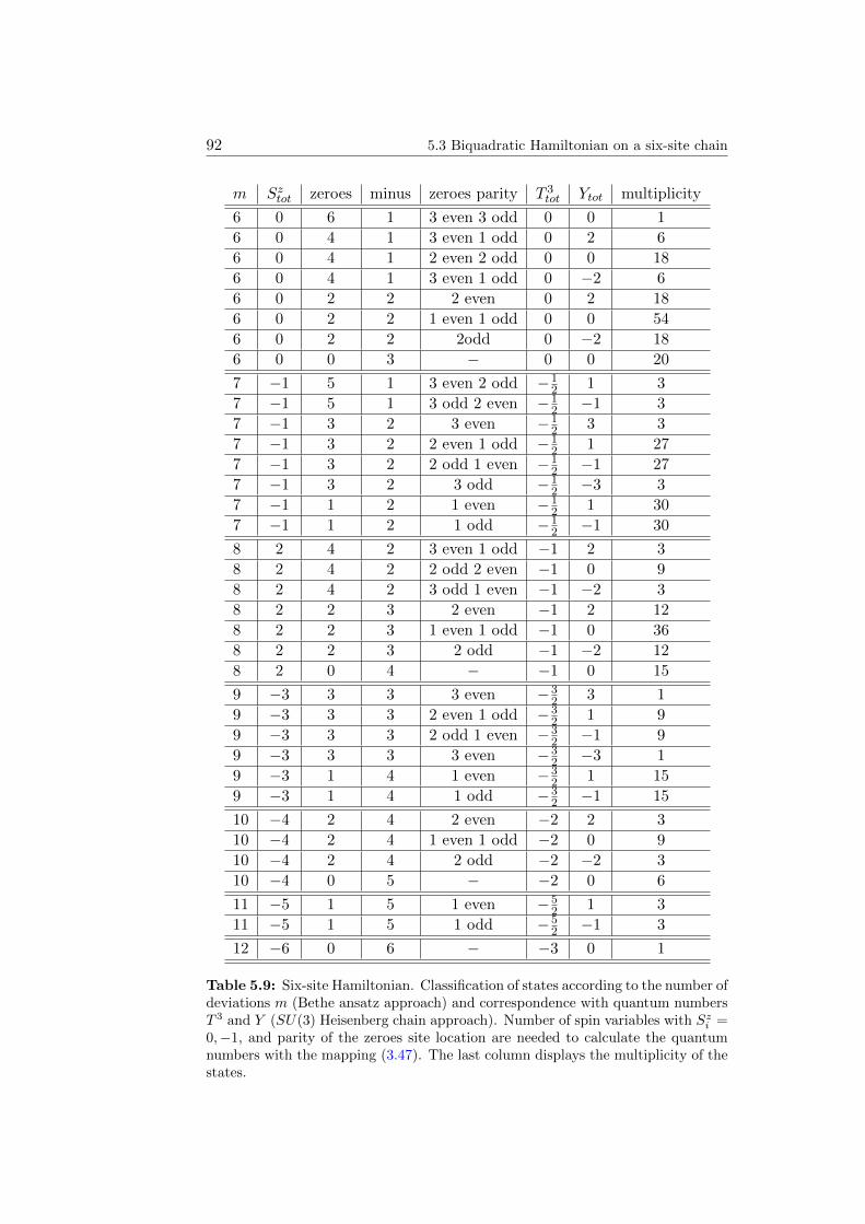
92 5.3 Biquadratic Hamiltonian on a six-site chain
m Sztot zeroes minus zeroes parity T 3tot Ytot multiplicity
6 0 6 1 3 even 3 odd 0 0 1
6 0 4 1 3 even 1 odd 0 2 6
6 0 4 1 2 even 2 odd 0 0 18
6 0 4 1 3 even 1 odd 0 −2 6
6 0 2 2 2 even 0 2 18
6 0 2 2 1 even 1 odd 0 0 54
6 0 2 2 2odd 0 −2 18
6 0 0 3 − 0 0 20
7 −1 5 1 3 even 2 odd −12 1 3
7 −1 5 1 3 odd 2 even −12 −1 3
7 −1 3 2 3 even −12 3 3
7 −1 3 2 2 even 1 odd −12 1 27
7 −1 3 2 2 odd 1 even −12 −1 27
7 −1 3 2 3 odd −12 −3 3
7 −1 1 2 1 even −12 1 30
7 −1 1 2 1 odd −12 −1 30
8 2 4 2 3 even 1 odd −1 2 3
8 2 4 2 2 odd 2 even −1 0 9
8 2 4 2 3 odd 1 even −1 −2 3
8 2 2 3 2 even −1 2 12
8 2 2 3 1 even 1 odd −1 0 36
8 2 2 3 2 odd −1 −2 12
8 2 0 4 − −1 0 15
9 −3 3 3 3 even −32 3 1
9 −3 3 3 2 even 1 odd −32 1 9
9 −3 3 3 2 odd 1 even −32 −1 9
9 −3 3 3 3 even −32 −3 1
9 −3 1 4 1 even −32 1 15
9 −3 1 4 1 odd −32 −1 15
10 −4 2 4 2 even −2 2 3
10 −4 2 4 1 even 1 odd −2 0 9
10 −4 2 4 2 odd −2 −2 3
10 −4 0 5 − −2 0 6
11 −5 1 5 1 even −52 1 3
11 −5 1 5 1 odd −52 −1 3
12 −6 0 6 − −3 0 1
Table 5.9: Six-site Hamiltonian. Classification of states according to the number ofdeviations m (Bethe ansatz approach) and correspondence with quantum numbersT 3 and Y (SU(3) Heisenberg chain approach). Number of spin variables with Szi =0,−1, and parity of the zeroes site location are needed to calculate the quantumnumbers with the mapping (3.47). The last column displays the multiplicity of thestates.
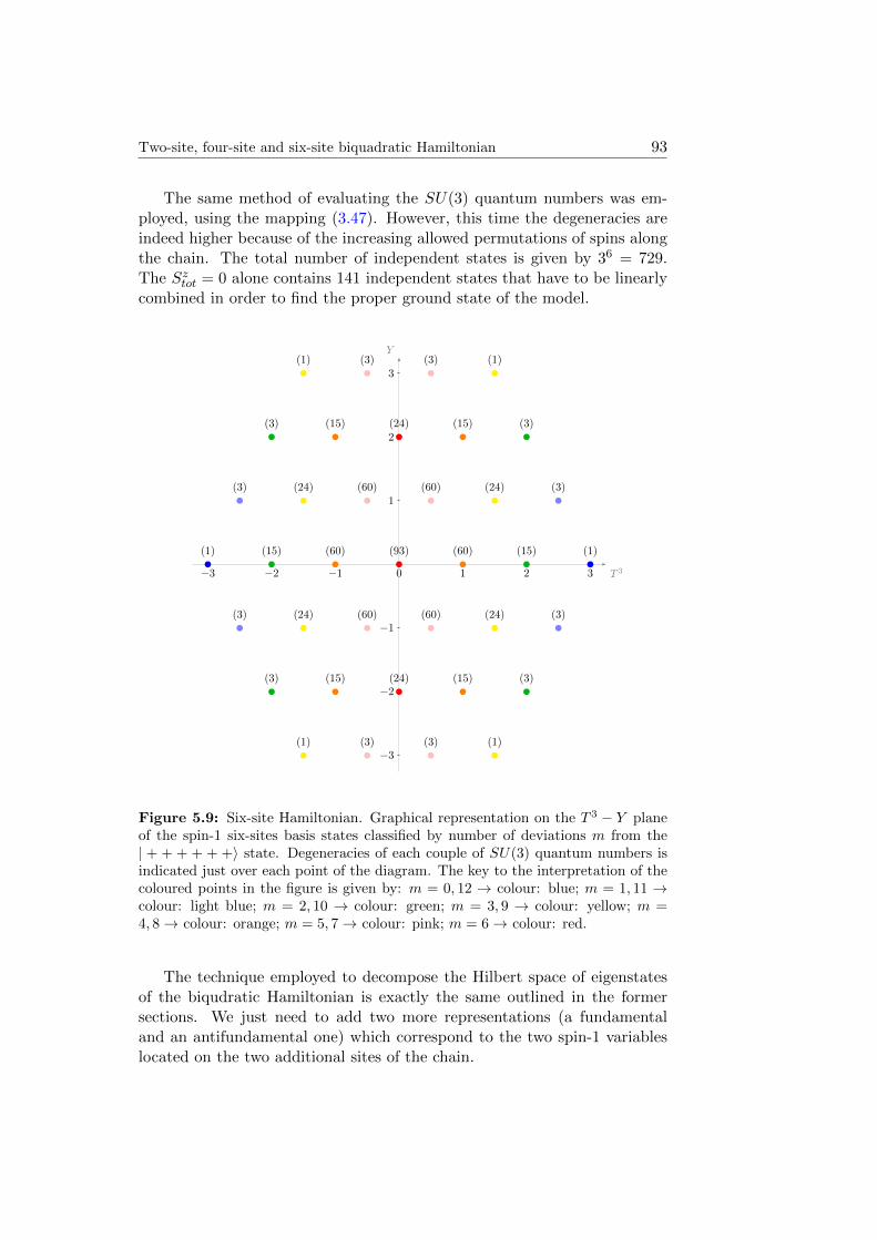
Two-site, four-site and six-site biquadratic Hamiltonian 93
The same method of evaluating the SU(3) quantum numbers was em-ployed, using the mapping (3.47). However, this time the degeneracies areindeed higher because of the increasing allowed permutations of spins alongthe chain. The total number of independent states is given by 36 = 729.The Sztot = 0 alone contains 141 independent states that have to be linearlycombined in order to find the proper ground state of the model.
T 3
Y
3210123
3
2
1
1
2
3
(1)(1)
(3)(3)
(3) (3)
(3)
(15)
(3)
(3)
(15)
(3)
(1)
(24)
(24)
(1)
(1)
(24)
(24)
(1)
(15)
(60)
(15)
(15)
(60)
(15)
(3)
(60)
(60)
(3)
(3)
(60)
(60)
(3)
(24)
(93)
(24)
1
Figure 5.9: Six-site Hamiltonian. Graphical representation on the T 3 − Y planeof the spin-1 six-sites basis states classified by number of deviations m from the| + + + + + +〉 state. Degeneracies of each couple of SU(3) quantum numbers isindicated just over each point of the diagram. The key to the interpretation of thecoloured points in the figure is given by: m = 0, 12 → colour: blue; m = 1, 11 →colour: light blue; m = 2, 10 → colour: green; m = 3, 9 → colour: yellow; m =4, 8→ colour: orange; m = 5, 7→ colour: pink; m = 6→ colour: red.
The technique employed to decompose the Hilbert space of eigenstatesof the biqudratic Hamiltonian is exactly the same outlined in the formersections. We just need to add two more representations (a fundamentaland an antifundamental one) which correspond to the two spin-1 variableslocated on the two additional sites of the chain.
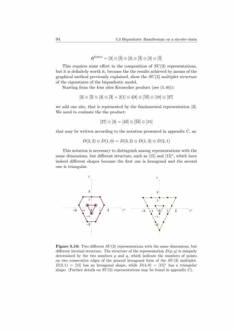
94 5.3 Biquadratic Hamiltonian on a six-site chain
H6sites = [3]⊗ [3]⊗ [3]⊗ [3]⊗ [3]⊗ [3]
This requires some effort in the composition of SU(3) representations,but it is definitely worth it, because the the results achieved by means of thegraphical method previously explained, show the SU(3) multiplet structureof the eigenstates of the biquadratic model.
Starting from the four sites Kronecker product (see (5.46)):
[3]⊗ [3]⊗ [3]⊗ [3] = 2[1]⊕ 4[8]⊕ [10]⊕ [10]⊕ [27]
we add one site, that is represented by the fundamental representation [3].We need to evaluate the the product:
[27]⊗ [3] = [42]⊕ [24]⊕ [15]
that may be written according to the notation presented in appendix C, as:
D(2, 2)⊗D(1, 0) = D(3, 2)⊕D(1, 3)⊕D(2, 1)
This notation is necessary to distinguish among representations with thesame dimensions, but different structure, such as [15] and [15]∗, which haveindeed different shapes because the first one is hexagonal and the secondone is triangular.
Figure 5.10: Two different SU(3) representations with the same dimensions, butdifferent internal structure. The structure of the representation D(p, q) is uniquelydetermined by the two numbers p and q, which indicate the numbers of pointson two consecutive edges of the general hexagonal form of the SU(3) multiplet.D(2, 1) = [15] has an hexagonal shape, while D(4, 0) = [15]∗ has a triangularshape. (Further details on SU(3) representations may be found in appendix C).
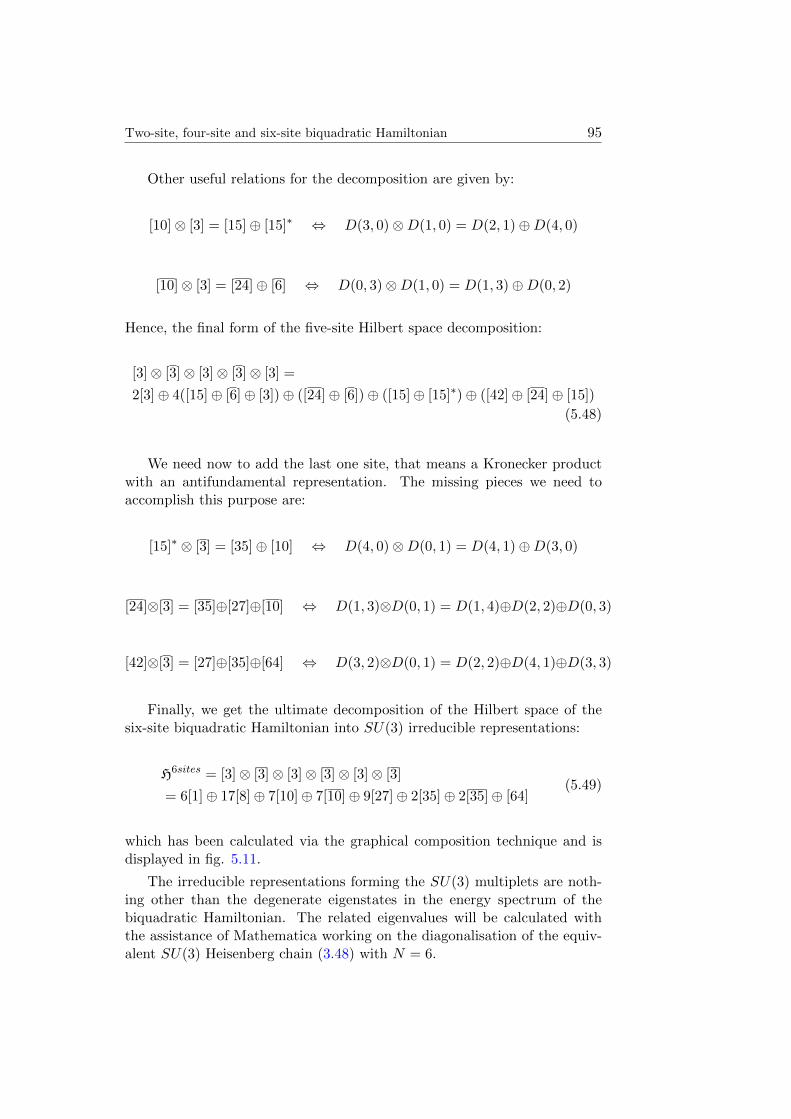
Two-site, four-site and six-site biquadratic Hamiltonian 95
Other useful relations for the decomposition are given by:
[10]⊗ [3] = [15]⊕ [15]∗ ⇔ D(3, 0)⊗D(1, 0) = D(2, 1)⊕D(4, 0)
[10]⊗ [3] = [24]⊕ [6] ⇔ D(0, 3)⊗D(1, 0) = D(1, 3)⊕D(0, 2)
Hence, the final form of the five-site Hilbert space decomposition:
[3]⊗ [3]⊗ [3]⊗ [3]⊗ [3] =
2[3]⊕ 4([15]⊕ [6]⊕ [3])⊕ ([24]⊕ [6])⊕ ([15]⊕ [15]∗)⊕ ([42]⊕ [24]⊕ [15])
(5.48)
We need now to add the last one site, that means a Kronecker productwith an antifundamental representation. The missing pieces we need toaccomplish this purpose are:
[15]∗ ⊗ [3] = [35]⊕ [10] ⇔ D(4, 0)⊗D(0, 1) = D(4, 1)⊕D(3, 0)
[24]⊗[3] = [35]⊕[27]⊕[10] ⇔ D(1, 3)⊗D(0, 1) = D(1, 4)⊕D(2, 2)⊕D(0, 3)
[42]⊗[3] = [27]⊕[35]⊕[64] ⇔ D(3, 2)⊗D(0, 1) = D(2, 2)⊕D(4, 1)⊕D(3, 3)
Finally, we get the ultimate decomposition of the Hilbert space of thesix-site biquadratic Hamiltonian into SU(3) irreducible representations:
H6sites = [3]⊗ [3]⊗ [3]⊗ [3]⊗ [3]⊗ [3]
= 6[1]⊕ 17[8]⊕ 7[10]⊕ 7[10]⊕ 9[27]⊕ 2[35]⊕ 2[35]⊕ [64](5.49)
which has been calculated via the graphical composition technique and isdisplayed in fig. 5.11.
The irreducible representations forming the SU(3) multiplets are noth-ing other than the degenerate eigenstates in the energy spectrum of thebiquadratic Hamiltonian. The related eigenvalues will be calculated withthe assistance of Mathematica working on the diagonalisation of the equiv-alent SU(3) Heisenberg chain (3.48) with N = 6.
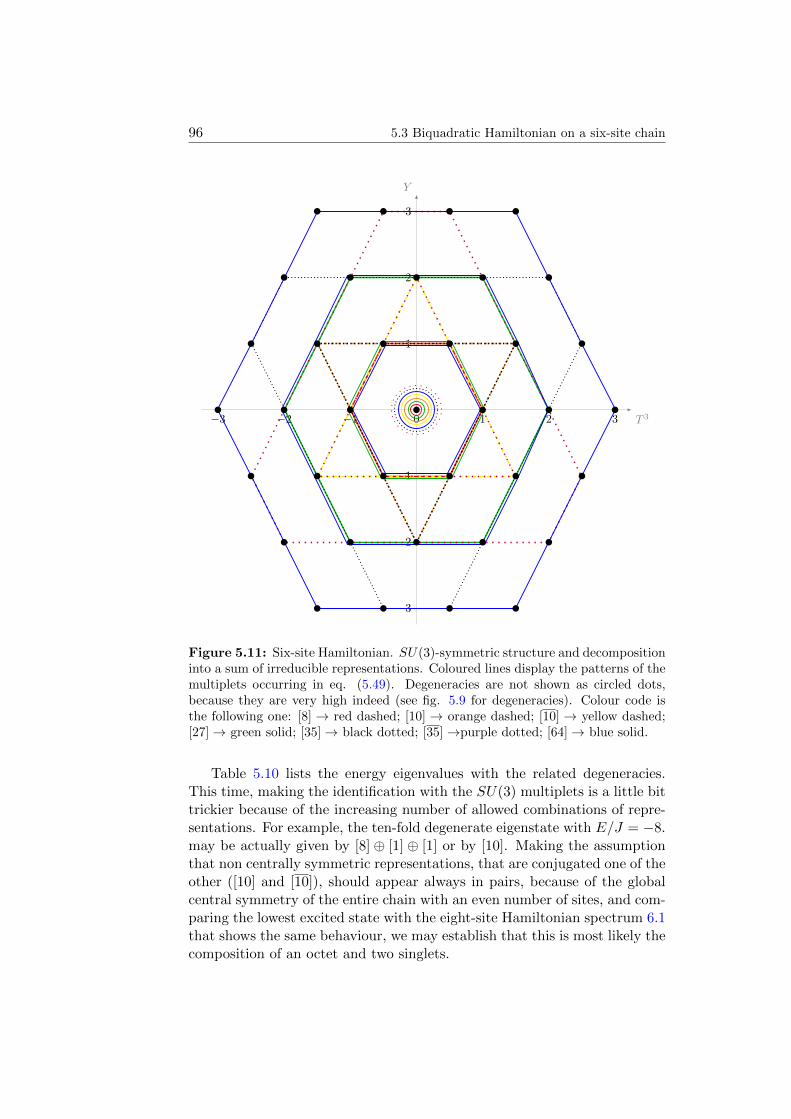
96 5.3 Biquadratic Hamiltonian on a six-site chain
T 3
Y
3210123
3
2
1
1
2
3
1
Figure 5.11: Six-site Hamiltonian. SU(3)-symmetric structure and decompositioninto a sum of irreducible representations. Coloured lines display the patterns of themultiplets occurring in eq. (5.49). Degeneracies are not shown as circled dots,because they are very high indeed (see fig. 5.9 for degeneracies). Colour code isthe following one: [8] → red dashed; [10] → orange dashed; [10] → yellow dashed;[27]→ green solid; [35]→ black dotted; [35]→purple dotted; [64]→ blue solid.
Table 5.10 lists the energy eigenvalues with the related degeneracies.This time, making the identification with the SU(3) multiplets is a little bittrickier because of the increasing number of allowed combinations of repre-sentations. For example, the ten-fold degenerate eigenstate with E/J = −8.may be actually given by [8] ⊕ [1] ⊕ [1] or by [10]. Making the assumptionthat non centrally symmetric representations, that are conjugated one of theother ([10] and [10]), should appear always in pairs, because of the globalcentral symmetry of the entire chain with an even number of sites, and com-paring the lowest excited state with the eight-site Hamiltonian spectrum 6.1that shows the same behaviour, we may establish that this is most likely thecomposition of an octet and two singlets.
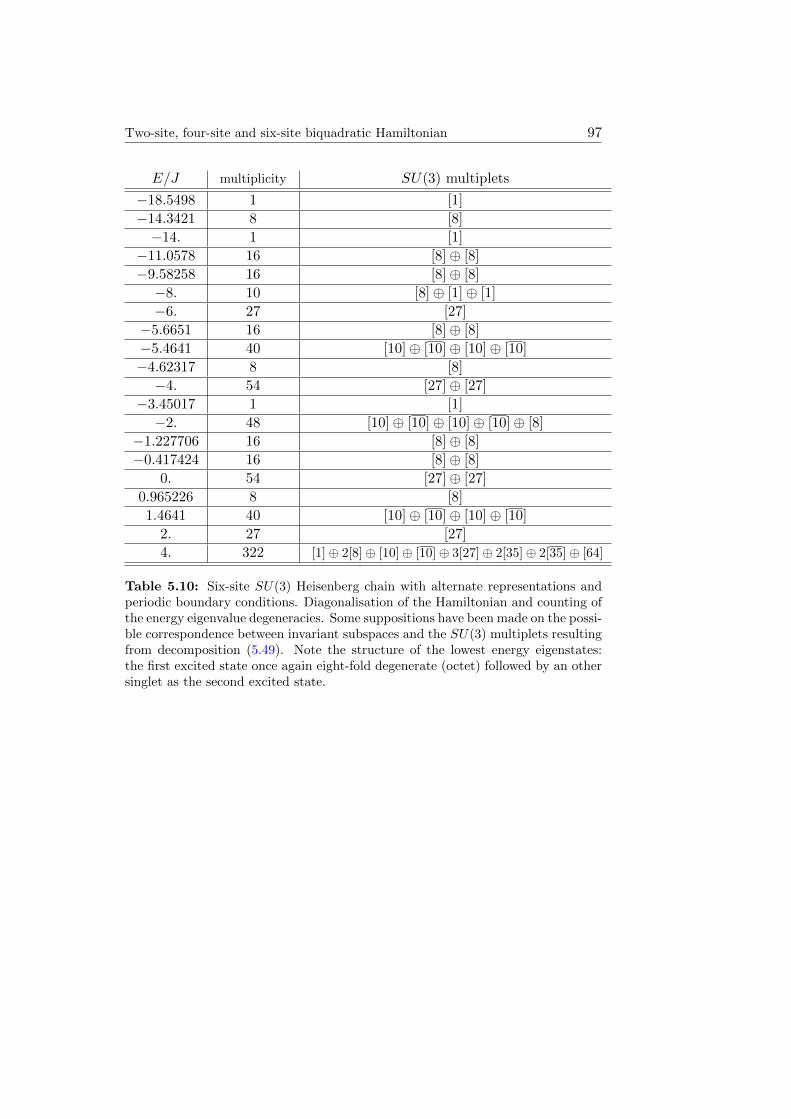
Two-site, four-site and six-site biquadratic Hamiltonian 97
E/J multiplicity SU(3) multiplets
−18.5498 1 [1]
−14.3421 8 [8]
−14. 1 [1]
−11.0578 16 [8]⊕ [8]
−9.58258 16 [8]⊕ [8]
−8. 10 [8]⊕ [1]⊕ [1]
−6. 27 [27]
−5.6651 16 [8]⊕ [8]
−5.4641 40 [10]⊕ [10]⊕ [10]⊕ [10]
−4.62317 8 [8]
−4. 54 [27]⊕ [27]
−3.45017 1 [1]
−2. 48 [10]⊕ [10]⊕ [10]⊕ [10]⊕ [8]
−1.227706 16 [8]⊕ [8]
−0.417424 16 [8]⊕ [8]
0. 54 [27]⊕ [27]
0.965226 8 [8]
1.4641 40 [10]⊕ [10]⊕ [10]⊕ [10]
2. 27 [27]
4. 322 [1]⊕ 2[8]⊕ [10]⊕ [10]⊕ 3[27]⊕ 2[35]⊕ 2[35]⊕ [64]
Table 5.10: Six-site SU(3) Heisenberg chain with alternate representations andperiodic boundary conditions. Diagonalisation of the Hamiltonian and counting ofthe energy eigenvalue degeneracies. Some suppositions have been made on the possi-ble correspondence between invariant subspaces and the SU(3) multiplets resultingfrom decomposition (5.49). Note the structure of the lowest energy eigenstates:the first excited state once again eight-fold degenerate (octet) followed by an othersinglet as the second excited state.

Chapter 6
Eight-site Hamiltonian andnew results
In this chapter we will deal with the eight-site biquadratic chain mainlyemploying a numerical approach, thanks to the assistance of Mathematica,which allows us to diagonalise the matrix representing the Hamiltonian op-erator, even though its dimension (38 × 38) becomes too high to evaluateeven the decomposition coefficients of the eigenvectors on the Hilbert spacecanonical basis.
We will focus our analysis on the ground state and the gap with thelowest excited states. It is clear that, since we are far away from the ther-modynamic limit, the ground state is single-degenerate, however the lowestexcited is a represented by an other singlet which will become degeneratewith it in the infinite-volume limit.
The remaining part is dedicated to the perturbation of the pure-biquadra-tic interaction by means of the introduction of a bilinear term, having theform of the usual spin-1 Heisenberg Hamiltonian. We will analyse theinfluence created by the additional term, which breaks the SU(3) symme-try of the model, leading to a splitting of the degenerate states of the bi-quadratic spectrum. We will examine at first small and then larger values ofthe coupling for the bilinear term, moving away from the biquadratic pointin the phase diagram, towards the two nearest known points, namely theantiferromagnetic-ferromagnetic phase transition (point D; Θ = 3
4π) and theTahkhtajan and Babudjian model (point B; π
4 ).
6.1 Comments on the ground state of the pure-biquadratic model
The ground state for the biquadratic spin-1 Hamiltonian in the infinite vol-ume limit is supposed to be doubly degenenerate [17, 26]. In fact, the purely
99
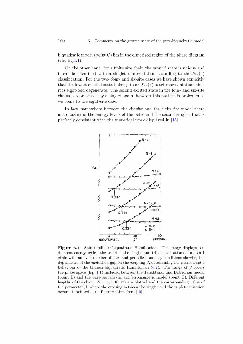
100 6.1 Comments on the ground state of the pure-biquadratic model
biquadratic model (point C) lies in the dimerised region of the phase diagram(cfr. fig.1.1).
On the other hand, for a finite size chain the ground state is unique andit can be identified with a singlet representation according to the SU(3)classification. For the two- four- and six-site cases we have shown explicitlythat the lowest excited state belongs to an SU(3) octet representation, thusit is eight-fold degenerate. The second excited state in the four- and six-sitechains is represented by a singlet again, however this pattern is broken oncewe come to the eight-site case.
In fact, somewhere between the six-site and the eight-site model thereis a crossing of the energy levels of the octet and the second singlet, that isperfectly consistent with the numerical work displayed in [15].
Figure 6.1: Spin-1 bilinear-biquadratic Hamiltonian. The image displays, ondifferent energy scales, the trend of the singlet and triplet excitations of a spin-1chain with an even number of sites and periodic boundary conditions showing thedependence of the excitation gap on the coupling β, determining the characteristicbehaviour of the bilinear-biquadratic Hamiltonian (6.2). The range of β coversthe phase space (fig. 1.1) included between the Tahkhtajan and Babudjian model(point B) and the pure-biquadratic antiferromagnetic model (point C). Differentlengths of the chain (N = 6, 8, 10, 12) are plotted and the corresponding value ofthe parameter β, where the crossing between the singlet and the triplet excitationoccurs, is pointed out. (Picture taken from [15]).
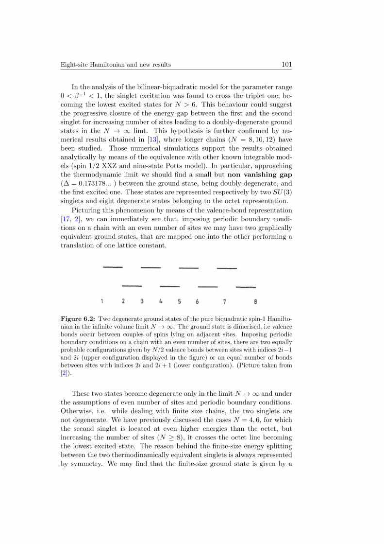
Eight-site Hamiltonian and new results 101
In the analysis of the bilinear-biquadratic model for the parameter range0 < β−1 < 1, the singlet excitation was found to cross the triplet one, be-coming the lowest excited states for N > 6. This behaviour could suggestthe progressive closure of the energy gap between the first and the secondsinglet for increasing number of sites leading to a doubly-degenerate groundstates in the N → ∞ limt. This hypothesis is further confirmed by nu-merical results obtained in [13], where longer chains (N = 8, 10, 12) havebeen studied. Those numerical simulations support the results obtainedanalytically by means of the equivalence with other known integrable mod-els (spin 1/2 XXZ and nine-state Potts model). In particular, approachingthe thermodynamic limit we should find a small but non vanishing gap(∆ = 0.173178... ) between the ground-state, being doubly-degenerate, andthe first excited one. These states are represented respectively by two SU(3)singlets and eight degenerate states belonging to the octet representation.
Picturing this phenomenon by means of the valence-bond representation[17, 2], we can immediately see that, imposing periodic boundary condi-tions on a chain with an even number of sites we may have two graphicallyequivalent ground states, that are mapped one into the other performing atranslation of one lattice constant.
Figure 6.2: Two degenerate ground states of the pure biquadratic spin-1 Hamilto-nian in the infinite volume limit N →∞. The ground state is dimerised, i.e valencebonds occur between couples of spins lying on adjacent sites. Imposing periodicboundary conditions on a chain with an even number of sites, there are two equallyprobable configurations given by N/2 valence bonds between sites with indices 2i−1and 2i (upper configuration displayed in the figure) or an equal number of bondsbetween sites with indices 2i and 2i+ 1 (lower configuration). (Picture taken from[2]).
These two states become degenerate only in the limit N →∞ and underthe assumptions of even number of sites and periodic boundary conditions.Otherwise, i.e. while dealing with finite size chains, the two singlets arenot degenerate. We have previously discussed the cases N = 4, 6, for whichthe second singlet is located at even higher energies than the octet, butincreasing the number of sites (N ≥ 8), it crosses the octet line becomingthe lowest excited state. The reason behind the finite-size energy splittingbetween the two thermodinamically equivalent singlets is always representedby symmetry. We may find that the finite-size ground state is given by a
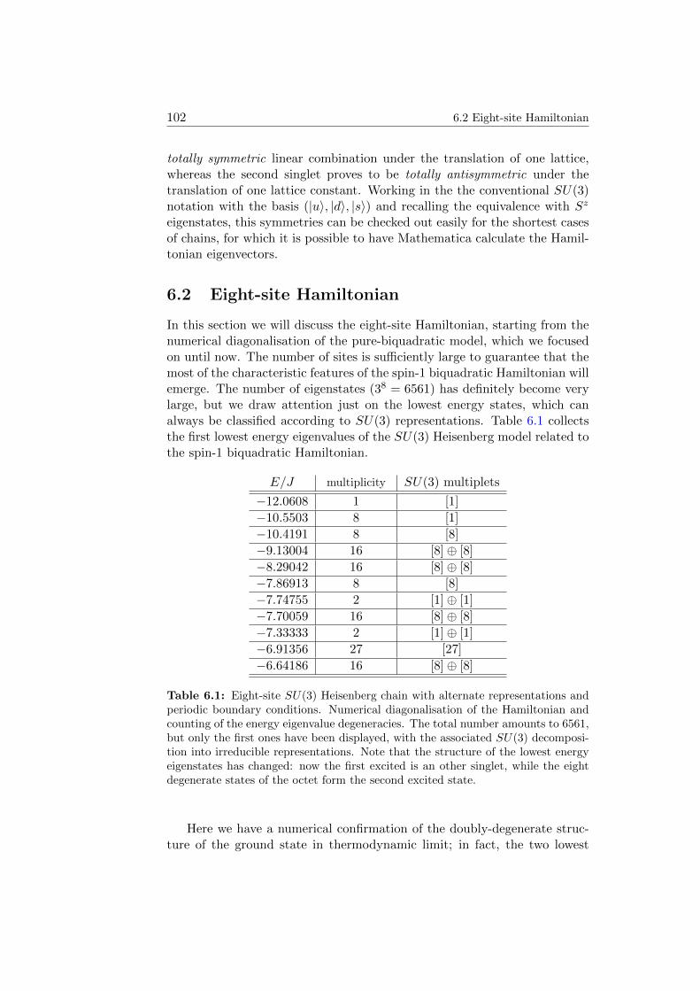
102 6.2 Eight-site Hamiltonian
totally symmetric linear combination under the translation of one lattice,whereas the second singlet proves to be totally antisymmetric under thetranslation of one lattice constant. Working in the the conventional SU(3)notation with the basis (|u〉, |d〉, |s〉) and recalling the equivalence with Sz
eigenstates, this symmetries can be checked out easily for the shortest casesof chains, for which it is possible to have Mathematica calculate the Hamil-tonian eigenvectors.
6.2 Eight-site Hamiltonian
In this section we will discuss the eight-site Hamiltonian, starting from thenumerical diagonalisation of the pure-biquadratic model, which we focusedon until now. The number of sites is sufficiently large to guarantee that themost of the characteristic features of the spin-1 biquadratic Hamiltonian willemerge. The number of eigenstates (38 = 6561) has definitely become verylarge, but we draw attention just on the lowest energy states, which canalways be classified according to SU(3) representations. Table 6.1 collectsthe first lowest energy eigenvalues of the SU(3) Heisenberg model related tothe spin-1 biquadratic Hamiltonian.
E/J multiplicity SU(3) multiplets
−12.0608 1 [1]
−10.5503 8 [1]
−10.4191 8 [8]
−9.13004 16 [8]⊕ [8]
−8.29042 16 [8]⊕ [8]
−7.86913 8 [8]
−7.74755 2 [1]⊕ [1]
−7.70059 16 [8]⊕ [8]
−7.33333 2 [1]⊕ [1]
−6.91356 27 [27]
−6.64186 16 [8]⊕ [8]
Table 6.1: Eight-site SU(3) Heisenberg chain with alternate representations andperiodic boundary conditions. Numerical diagonalisation of the Hamiltonian andcounting of the energy eigenvalue degeneracies. The total number amounts to 6561,but only the first ones have been displayed, with the associated SU(3) decomposi-tion into irreducible representations. Note that the structure of the lowest energyeigenstates has changed: now the first excited is an other singlet, while the eightdegenerate states of the octet form the second excited state.
Here we have a numerical confirmation of the doubly-degenerate struc-ture of the ground state in thermodynamic limit; in fact, the two lowest
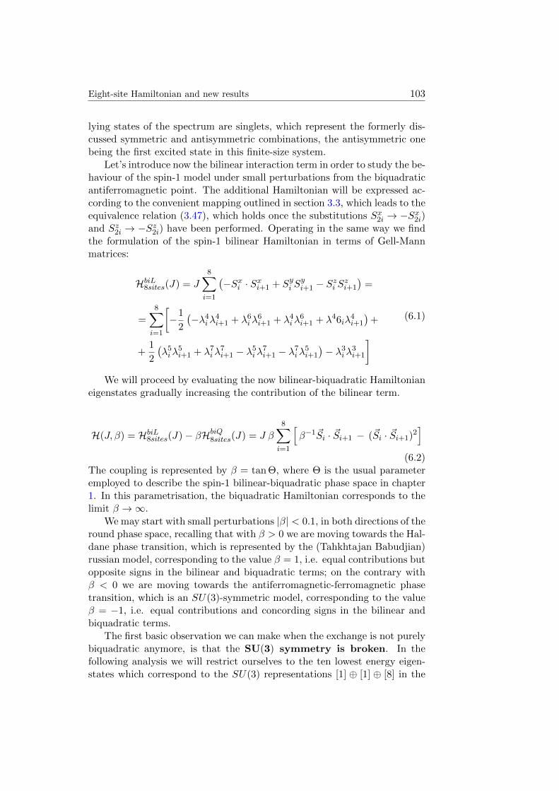
Eight-site Hamiltonian and new results 103
lying states of the spectrum are singlets, which represent the formerly dis-cussed symmetric and antisymmetric combinations, the antisymmetric onebeing the first excited state in this finite-size system.
Let’s introduce now the bilinear interaction term in order to study the be-haviour of the spin-1 model under small perturbations from the biquadraticantiferromagnetic point. The additional Hamiltonian will be expressed ac-cording to the convenient mapping outlined in section 3.3, which leads to theequivalence relation (3.47), which holds once the substitutions Sx2i → −Sx2i)and Sz2i → −Sz2i) have been performed. Operating in the same way we findthe formulation of the spin-1 bilinear Hamiltonian in terms of Gell-Mannmatrices:
HbiL8sites(J) = J8∑i=1
(−Sxi · Sxi+1 + Syi S
yi+1 − Szi Szi+1
)=
=8∑i=1
[−1
2
(−λ4iλ4i+1 + λ6iλ
6i+1 + λ4iλ
6i+1 + λ46iλ
4i+1
)+
+1
2
(λ5iλ
5i+1 + λ7iλ
7i+1 − λ5iλ7i+1 − λ7iλ5i+1
)− λ3iλ3i+1
](6.1)
We will proceed by evaluating the now bilinear-biquadratic Hamiltonianeigenstates gradually increasing the contribution of the bilinear term.
H(J, β) = HbiL8sites(J)− βHbiQ8sites(J) = J β8∑i=1
[β−1~Si · ~Si+1 − (~Si · ~Si+1)
2]
(6.2)The coupling is represented by β = tan Θ, where Θ is the usual parameteremployed to describe the spin-1 bilinear-biquadratic phase space in chapter1. In this parametrisation, the biquadratic Hamiltonian corresponds to thelimit β →∞.
We may start with small perturbations |β| < 0.1, in both directions of theround phase space, recalling that with β > 0 we are moving towards the Hal-dane phase transition, which is represented by the (Tahkhtajan Babudjian)russian model, corresponding to the value β = 1, i.e. equal contributions butopposite signs in the bilinear and biquadratic terms; on the contrary withβ < 0 we are moving towards the antiferromagnetic-ferromagnetic phasetransition, which is an SU(3)-symmetric model, corresponding to the valueβ = −1, i.e. equal contributions and concording signs in the bilinear andbiquadratic terms.
The first basic observation we can make when the exchange is not purelybiquadratic anymore, is that the SU(3) symmetry is broken. In thefollowing analysis we will restrict ourselves to the ten lowest energy eigen-states which correspond to the SU(3) representations [1] ⊕ [1] ⊕ [8] in the
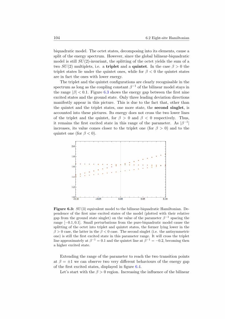
104 6.2 Eight-site Hamiltonian
biquadratic model. The octet states, decomposing into its elements, cause asplit of the energy spectrum. However, since the global bilinear-biquadraticmodel is still SU(2)-invariant, the splitting of the octet yields the sum of atwo SU(2) multiplets, i.e. a triplet and a quintet. In the case β > 0 thetriplet states lie under the quintet ones, while for β < 0 the quintet statesare in fact the ones with lower energy.
The triplet and the quintet configurations are clearly recognisable in thespectrum as long as the coupling constant β−1 of the bilinear model stays inthe range |β| < 0.1. Figure 6.3 shows the energy gap between the first nineexcited states and the ground state. Only three leading deviation directionsmanifestly appear in this picture. This is due to the fact that, other thanthe quintet and the triplet states, one more state, the second singlet, isaccounted into these pictures. Its energy does not cross the two lower linesof the triplet and the quintet, for β > 0 and β < 0 respectively. Thus,it remains the first excited state in this range of the parameter. As |β−1|increases, its value comes closer to the triplet one (for β > 0) and to thequintet one (for β < 0).
Figure 6.3: SU(3) equivalent model to the bilinear-biquadratic Hamiltonian. De-pendence of the first nine excited states of the model (plotted with their relativegap from the ground state singlet) on the value of the parameter β−1 spacing therange [−0.1, 0.1]. Small perturbations from the pure-biquadratic model cause thesplitting of the octet into triplet and quintet states, the former lying lower in theβ > 0 case, the latter in the β < 0 case. The second singlet (i.e. the antisymmetricone) is still the first excited state in this parameter range. It will cross the tripletline approximately at β−1 = 0.1 and the quintet line at β−1 = −0.2, becoming thena higher excited state.
Extending the range of the parameter to reach the two transition pointsat β = ±1 we can observe two very different behaviours of the energy gapof the first excited states, displayed in figure 6.4.
Let’s start with the β > 0 region. Increasing the influence of the bilinear
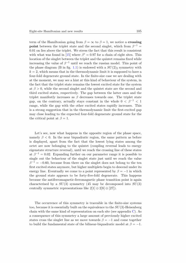
Eight-site Hamiltonian and new results 105
term of the Hamiltonian going from β =∞ to β = 1, we notice a crossingpoint between the triplet state and the second singlet, which from β−1 =0.01 on lies above the triplet. We stress the fact that this result is consistentwith what was found in [15] where β∗ = 0.97 for a chain of eight sites. Thislocation of the singlet between the triplet and the quintet remains fixed whileincreasing the value of β−1 until we reach the russian model. This point ofthe phase diagram (B in fig. 1.1) is endowed with a SU(2)2 symmetry withk = 2, which means that in the thermodynamic limit it is supposed to have afour-fold degenerate ground state. In the finite-size case we are dealing withat the moment, we may see a hint at this kind of behaviour of the system, inthe fact that the triplet state remains the lowest excited state for the systemat β > 0, while the second singlet and the quintet state are the second andthird excited states, respectively. The gap between the latter ones and thetriplet manifestly increases as β decreases towards one. The triplet stategap, on the contrary, actually stays constant in the whole 0 < β−1 < 1range, while the gap with the other excited states rapidly increases. Thisis a strong suggestion that in the thermodynamic limit the first-excited gapmay close leading to the expected four-fold degenerate ground state for thethe critical point at β = 1.
Let’s see, now what happens in the opposite region of the phase space,namely β < 0. In the near biquadratic region, the same pattern as beforeis displayed, apart from the fact that the lowest lying states among theoctet are now belonging to the quintet (coupling reversal leads to energyeigenstate structure reversal), until we reach the crossing line of these statesat β−1 = 0.02. Expanding further on our parameter range it is possible tosingle out the behaviour of the singlet state just until we reach the valueβ−1 = −0.60, because from there on the singlet does not belong to the tenfirst excited states anymore, but higher multiplets begin to descend under itsenergy line. Eventually we come to a point represented by β = −1 in whichthe ground state appears to be forty-five-fold degenerate. This happensbecause the antiferromagnetic-ferromagnetic phase transition point is againcharacterised by a SU(3) symmetry (45 may be decomposed into SU(3)centrally symmetric representations like 2[1]⊕ 2[8]⊕ [27]).
The occurrence of this symmetry is traceable in the finite-size systemstoo, because it is essentially built on the equivalence to the SU(3)-Heisenbergchain with the same kind of representation on each site (see appendix C). Asa consequence of this symmetry a large amount of previously higher excitedstates cross the singlet line as we move towards β = −1 and come togetherto build the fundamental state of the bilinear-biquadratic model at β = −1.
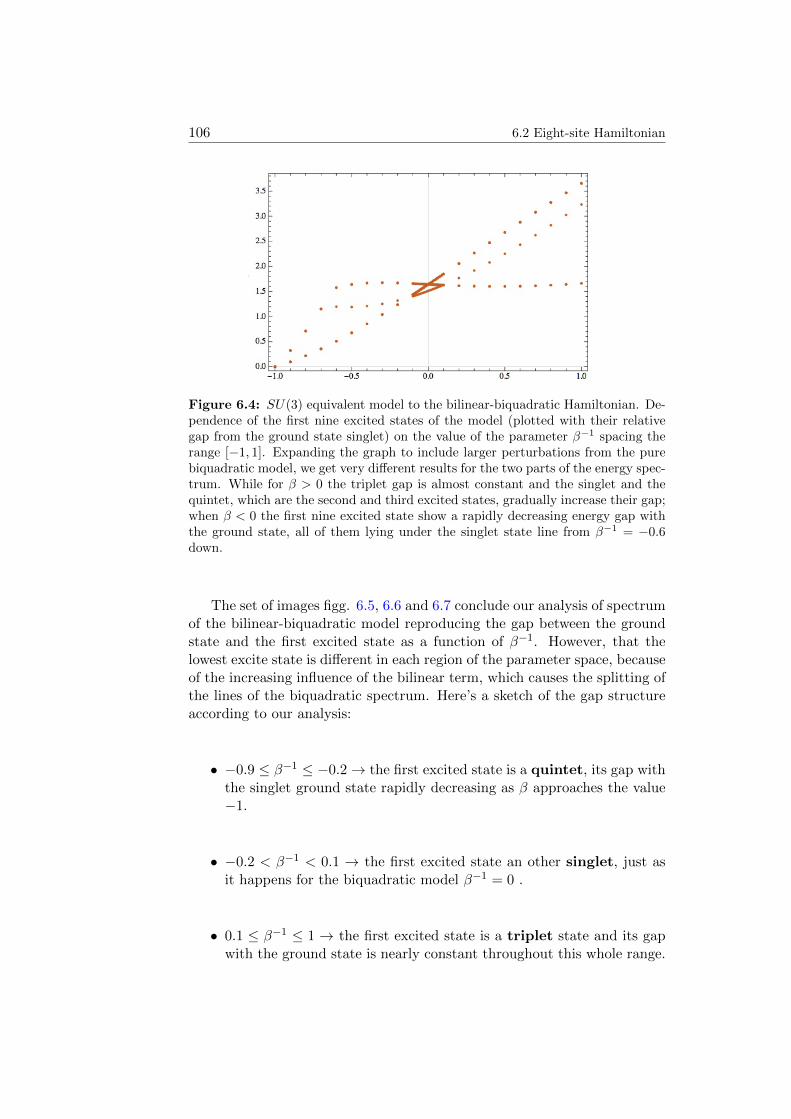
106 6.2 Eight-site Hamiltonian
Figure 6.4: SU(3) equivalent model to the bilinear-biquadratic Hamiltonian. De-pendence of the first nine excited states of the model (plotted with their relativegap from the ground state singlet) on the value of the parameter β−1 spacing therange [−1, 1]. Expanding the graph to include larger perturbations from the purebiquadratic model, we get very different results for the two parts of the energy spec-trum. While for β > 0 the triplet gap is almost constant and the singlet and thequintet, which are the second and third excited states, gradually increase their gap;when β < 0 the first nine excited state show a rapidly decreasing energy gap withthe ground state, all of them lying under the singlet state line from β−1 = −0.6down.
The set of images figg. 6.5, 6.6 and 6.7 conclude our analysis of spectrumof the bilinear-biquadratic model reproducing the gap between the groundstate and the first excited state as a function of β−1. However, that thelowest excite state is different in each region of the parameter space, becauseof the increasing influence of the bilinear term, which causes the splitting ofthe lines of the biquadratic spectrum. Here’s a sketch of the gap structureaccording to our analysis:
• −0.9 ≤ β−1 ≤ −0.2→ the first excited state is a quintet, its gap withthe singlet ground state rapidly decreasing as β approaches the value−1.
• −0.2 < β−1 < 0.1 → the first excited state an other singlet, just asit happens for the biquadratic model β−1 = 0 .
• 0.1 ≤ β−1 ≤ 1 → the first excited state is a triplet state and its gapwith the ground state is nearly constant throughout this whole range.
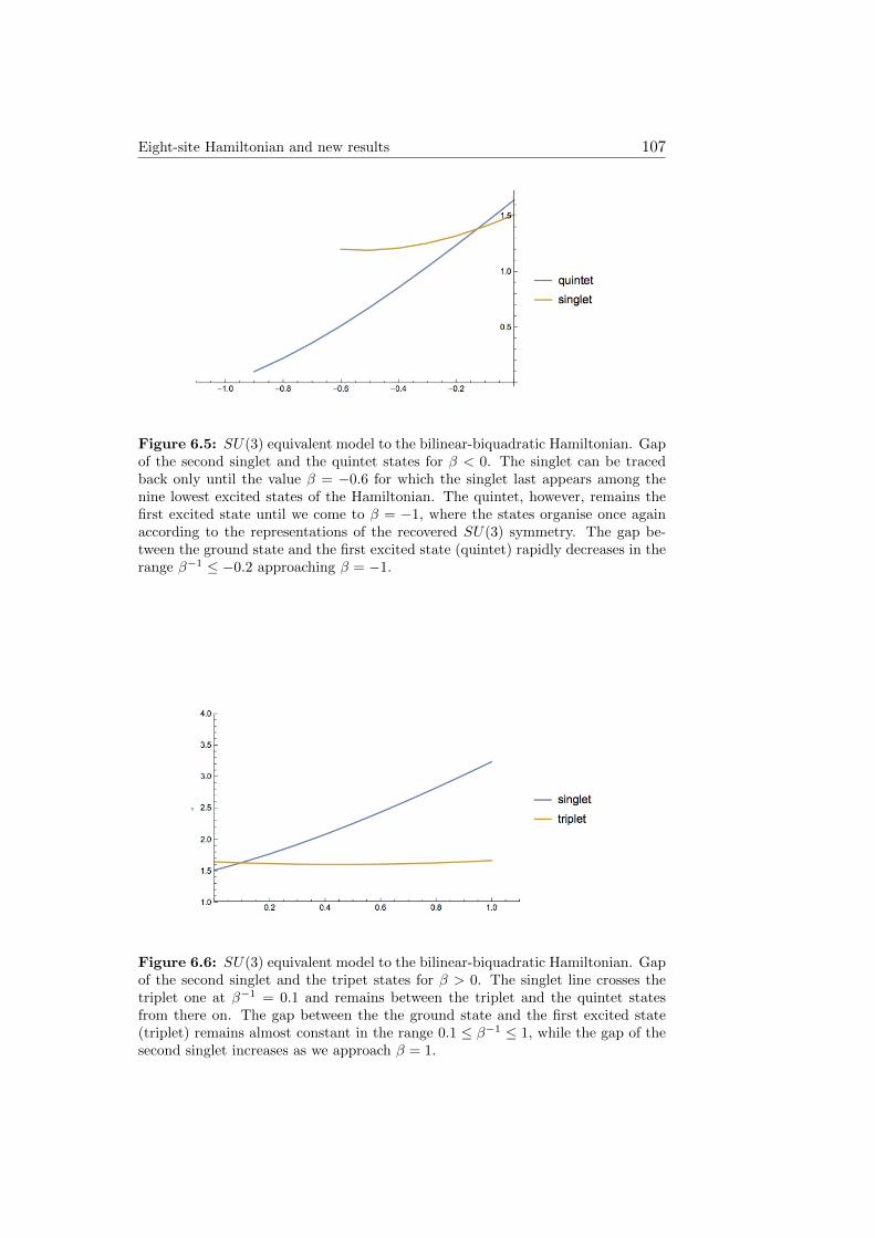
Eight-site Hamiltonian and new results 107
Figure 6.5: SU(3) equivalent model to the bilinear-biquadratic Hamiltonian. Gapof the second singlet and the quintet states for β < 0. The singlet can be tracedback only until the value β = −0.6 for which the singlet last appears among thenine lowest excited states of the Hamiltonian. The quintet, however, remains thefirst excited state until we come to β = −1, where the states organise once againaccording to the representations of the recovered SU(3) symmetry. The gap be-tween the ground state and the first excited state (quintet) rapidly decreases in therange β−1 ≤ −0.2 approaching β = −1.
Figure 6.6: SU(3) equivalent model to the bilinear-biquadratic Hamiltonian. Gapof the second singlet and the tripet states for β > 0. The singlet line crosses thetriplet one at β−1 = 0.1 and remains between the triplet and the quintet statesfrom there on. The gap between the the ground state and the first excited state(triplet) remains almost constant in the range 0.1 ≤ β−1 ≤ 1, while the gap of thesecond singlet increases as we approach β = 1.
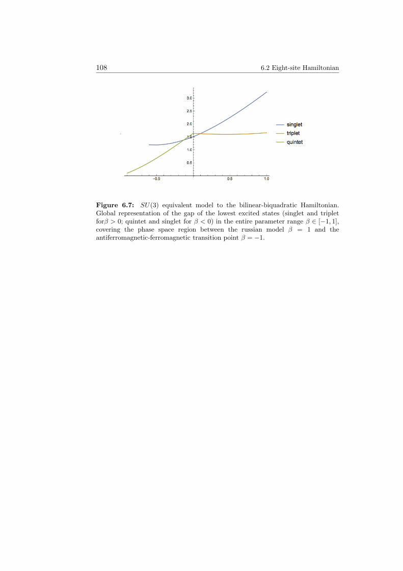
108 6.2 Eight-site Hamiltonian
Figure 6.7: SU(3) equivalent model to the bilinear-biquadratic Hamiltonian.Global representation of the gap of the lowest excited states (singlet and tripletforβ > 0; quintet and singlet for β < 0) in the entire parameter range β ∈ [−1, 1],covering the phase space region between the russian model β = 1 and theantiferromagnetic-ferromagnetic transition point β = −1.
Appendix A
Spin-1 Representations
The main topics dealt with in this thesis lay their foundations on spin-1 chains, which are essentially one dimensional models, where the relevantinteractions occur among spin variables positioned on each locus of the chain.This appendix tries to give a quick overview of the very basic properties ofthe spin-1 representations.
It is crucial to have a full understanding of the elementary propertiesof spin-1 operators on each site, because we will then consider a system ofspin variables interacting through a Hamiltonian, that connects the variousspins belonging to the chain. This results into a very large Hilbert space forthe system under consideration, which is essentially built up by Kroneckerproducts of representations of spin-1, as many as the number of sites on thechain.
A primary aim of this appendix is trying to establish a conventionalnotation, which we will follow consistently throughout the whole work.
A.1 Spin variables
Spin is an intrinsic degree of freedom of fundamental particles, which spon-taneously arises in the definition of fields behaviour under the action of therotation group. Therefore, spin may be thought as an intrinsic angular mo-mentum of elementary particles, which acts differently on each type of field,modifying the field form by means of position independent operators.
Different kinds of fields transform according to different types of spinrepresentations; namely spinor fields transform under the fundamental rep-resentation, meanwhile vector fields transform under the spin-1 one repre-sentation. This is the reason why vector fields are essentially employed todescribe spin-1 particles.
Different representations correspond to different operators and matrixdimensions, but with one underlying common feature, that is determined bythe universal behaviour of operators under commutation. The spin relation
109
110 A.2 Spin-1 operators
with angular momentum appears immediately clear when we check that thecommutation relations among spin group generators obey the SU(2) Liealgebra, that is exactly the same algebra as the rotation group SO(3).
This is the physical context in which spin emerges, but for our purposeswe shall focus on spin degrees of freedom only, separately from the otherphysical features related to particles.
A.2 Spin-1 operators
The spin-1 operators form a representation of the spin group of dimensionthree and are related to classical variables, which can take on three differentvalues, which we conventionally set to −1, 0,+1. The three cartesian com-ponents of the spin vector are conventionally represented by 3× 3 matrices:
Sx =1√2
(0 1 01 0 10 1 0
)Sy =
1√2
(0 −i 0i 0 −i0 i 0
)Sz =
(1 0 00 0 00 0 −1
)(A.1)
We may interpret the generators of the spin group as the three hermitiantraceless generators of the special unitary group SU(2), which is isomorphicto the rotations group in three dimensions SO(3). They, in fact, obey thesame Lie algebra, that has the following commutation relations:
[Sα, Sβ] = i εαβγSγ with α, β, γ = x, y, z (A.2)
We may introduce two new operators:
S± = Sx ± iSy(S±)†
= S∓ (A.3)
S+ =√
2
(0 1 00 0 10 0 0
)S− =
√2
(0 0 01 0 00 1 0
)(A.4)
which we call ladder operators, since their action on the eigenstates of Sz
has the effect of respectively raising or lowering by one unity the eigenvalueof Sz.
S+ |+〉 = 0 S+ |0〉 =√
2 |+〉 S+ |−〉 =√
2 |0〉S− |+〉 =
√2 |0〉 S− |0〉 =
√2 |−〉 S− |−〉 = 0
(A.5)
This property can be seen immediately by the following commutation rules,which may equally be taken as a definition of the SU(2) group:
[Sz, S±] = ±S± and [S+, S−] = 2Sz (A.6)
Since none of the generators commute with the others, we may indiffer-ently represent the states on a basis of eigenstates of a single one of the three
Spin-1 Representations 111
generators. It is convenient to choose Sz, which is diagonal with eigenvaluesλ = 0,±1. Therefore, we can decompose a generic state on the followingbasis, which is the canonical basis:
|+〉 =
100
|0〉 =
010
|−〉 =
001
(A.7)
The formerly outlined representation of the spin-1 operators is the bestphysical picture and usually the most widely employed. However, we maychoose different representations as long as they satisfy the same commuta-tion rules and, thus, the same Lie algebra, given by (A.2).
An other useful spin representation, which spontaneously arise from theinterpretation of spin as a rotation group, may be given by the antisymmetricgenerators of rotations in three dimensions times i~:
S1 = i~
(0 0 00 0 −10 1 0
)S2 = i~
( 0 0 10 0 0−1 0 0
)S3 = i~
(0 −1 01 0 00 0 0
)(A.8)
(In order to make them dimensionless we may drop the ~ dependence). Now,since all of the three matrices are non-diagonal, the eigenvalues of them beingλ = 0,±1, we may write down the eigenstates of S3 as linear combinationsof the canonical basis vectors in the following way:
|+〉 =1√2
−i10
|0〉 =
001
|−〉 =1√2
i10
(A.9)
This choice may be not very practical as long as we need to classify thestates according to the Sz eigenvalues, because we have to deal with linearcombinations, but it turns out to be a very useful representation to prove theequivalence of the biquadratic Hamiltonian with an SU(3) spin chain withalternate fundamental and antifundamental representations. (See AppendixC)
Eventually, let’s introduce one last spin representation which has beenmassively employed throughout this work, even though it is not really wide-spread. However, it allows an immediate classification of eigenstates of aspin chain because Sz has a diagonal form exactly corresponding to thethird Gell-Mann matrix. (see Appendix B and sections 3.3 and 3.4)
Sx =1√2
(0 0 10 0 11 1 0
)Sy =
1√2
(0 0 −i0 0 ii −i 0
)Sz =
(1 0 00 −1 00 0 0
)(A.10)
112 A.3 SU(2)-multiplets
The eigenvalues and eigenstates of Sz are exactly the same as (A.7), butthey appear in a slightly different order on the canonical basis:
|+〉 =
100
|0〉 =
001
|−〉 =
010
(A.11)
The same definitions (A.3), (A.4) and considerations (A.5) about theladder operators apply also in this case, with:
S+ =√
2
(0 0 10 0 00 1 0
)S− =
√2
(0 0 00 0 11 0 0
)(A.12)
We may check that the commutation relations (A.6) and (A.2) still hold too.
A.3 SU(2)-multiplets
SU(2) is a continuous symmetry group of dimension 22−1 = 3, isomorphic tothe rotations group in three dimensions, SO(3). Their common Lie algebrais built upon three generators, none of which commute with the others, asestablished by (A.2). The corresponding maximum number of commutingoperators, that defines the group rank is thus one. By Racach theorem wehave only one Casimir operator, that is:
S2 = (Sx)2 + (Sy)2 + (Sz)2 , (A.13)
which is a bilinear function of all the generators having the property of com-muting with all the former and thus with all the elements of the symmetrygroup.
Now we may start a classification of the SU(2)-symmetric states bylabelling them with the corresponding S2 eigenvalue.
The problem that arises in this picture is that S2 eigenvalues are notsufficient to point out a unique state, because in the generic representationof spin S, S2 eigenstates are (2S + 1)-fold degenerate. These 2S + 1 statestransform among themselves under the action of the ladder operator S+
and S−, closing the SU(2) algebra (A.2). The set of degenerate stateswhich transform among themselves under the action of a symmetry groupform an invariant subspace, called a multiplet. The Casimir operators of agroup uniquely characterize the multiplets.
Focusing on the particular case S = 1, we find three different eigenstates,each of them with an eigenvalue of S2 = S(S + 1) = 2, but we are allowedto label them thanks to an other good quantum number, which has beenchosen to be the Sz eigenvalue. They turn out to be:
|+〉 =∣∣S2 = 2, Sz = +1
⟩| 0 〉 =
∣∣S2 = 2, Sz = 0⟩
|−〉 =∣∣S2 = 2, Sz = −1
⟩ (A.14)
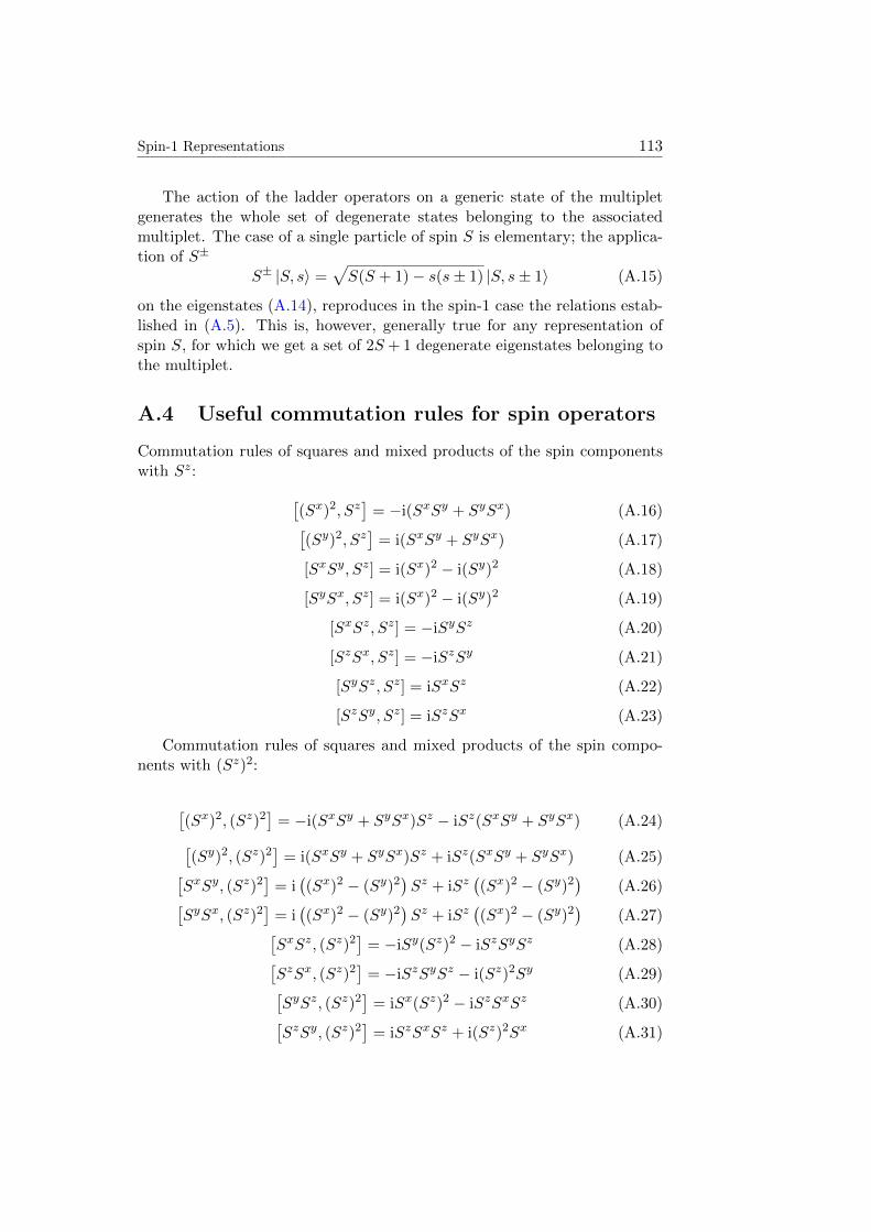
Spin-1 Representations 113
The action of the ladder operators on a generic state of the multipletgenerates the whole set of degenerate states belonging to the associatedmultiplet. The case of a single particle of spin S is elementary; the applica-tion of S±
S± |S, s〉 =√S(S + 1)− s(s± 1) |S, s± 1〉 (A.15)
on the eigenstates (A.14), reproduces in the spin-1 case the relations estab-lished in (A.5). This is, however, generally true for any representation ofspin S, for which we get a set of 2S + 1 degenerate eigenstates belonging tothe multiplet.
A.4 Useful commutation rules for spin operators
Commutation rules of squares and mixed products of the spin componentswith Sz: [
(Sx)2, Sz]
= −i(SxSy + SySx) (A.16)[(Sy)2, Sz
]= i(SxSy + SySx) (A.17)
[SxSy, Sz] = i(Sx)2 − i(Sy)2 (A.18)
[SySx, Sz] = i(Sx)2 − i(Sy)2 (A.19)
[SxSz, Sz] = −iSySz (A.20)
[SzSx, Sz] = −iSzSy (A.21)
[SySz, Sz] = iSxSz (A.22)
[SzSy, Sz] = iSzSx (A.23)
Commutation rules of squares and mixed products of the spin compo-nents with (Sz)2:
[(Sx)2, (Sz)2
]= −i(SxSy + SySx)Sz − iSz(SxSy + SySx) (A.24)[
(Sy)2, (Sz)2]
= i(SxSy + SySx)Sz + iSz(SxSy + SySx) (A.25)[SxSy, (Sz)2
]= i((Sx)2 − (Sy)2
)Sz + iSz
((Sx)2 − (Sy)2
)(A.26)[
SySx, (Sz)2]
= i((Sx)2 − (Sy)2
)Sz + iSz
((Sx)2 − (Sy)2
)(A.27)[
SxSz, (Sz)2]
= −iSy(Sz)2 − iSzSySz (A.28)[SzSx, (Sz)2
]= −iSzSySz − i(Sz)2Sy (A.29)[
SySz, (Sz)2]
= iSx(Sz)2 − iSzSxSz (A.30)[SzSy, (Sz)2
]= iSzSxSz + i(Sz)2Sx (A.31)

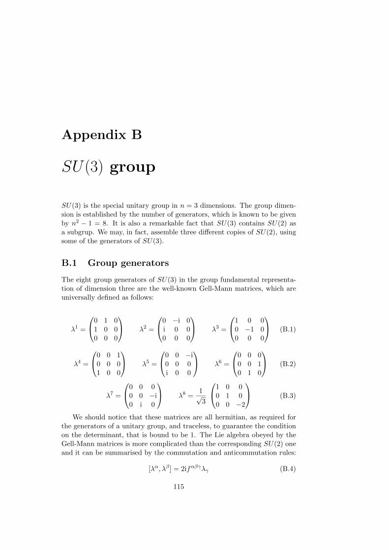
Appendix B
SU(3) group
SU(3) is the special unitary group in n = 3 dimensions. The group dimen-sion is established by the number of generators, which is known to be givenby n2 − 1 = 8. It is also a remarkable fact that SU(3) contains SU(2) asa subgrup. We may, in fact, assemble three different copies of SU(2), usingsome of the generators of SU(3).
B.1 Group generators
The eight group generators of SU(3) in the group fundamental representa-tion of dimension three are the well-known Gell-Mann matrices, which areuniversally defined as follows:
λ1 =
0 1 01 0 00 0 0
λ2 =
0 −i 0i 0 00 0 0
λ3 =
1 0 00 −1 00 0 0
(B.1)
λ4 =
0 0 10 0 01 0 0
λ5 =
0 0 −i0 0 0i 0 0
λ6 =
0 0 00 0 10 1 0
(B.2)
λ7 =
0 0 00 0 −i0 i 0
λ8 =1√3
1 0 00 1 00 0 −2
(B.3)
We should notice that these matrices are all hermitian, as required forthe generators of a unitary group, and traceless, to guarantee the conditionon the determinant, that is bound to be 1. The Lie algebra obeyed by theGell-Mann matrices is more complicated than the corresponding SU(2) oneand it can be summarised by the commutation and anticommutation rules:
[λα, λβ] = 2ifαβγλγ (B.4)
115
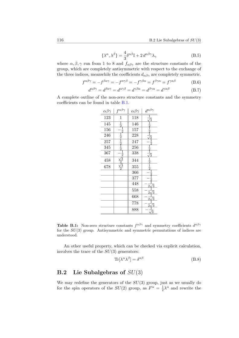
116 B.2 Lie Subalgebras of SU(3)
λα, λβ =4
3δαβI + 2 dαβγλγ (B.5)
where α, β, γ run from 1 to 8 and fαβγ are the structure constants of thegroup, which are completely antisymmetric with respect to the exchange ofthe three indices, meanwhile the coefficients dαβγ are completely symmetric.
fαβγ = −fβαγ = −fαγβ = −fγβα = fβγα = fγαβ (B.6)
dαβγ = dβαγ = dαγβ = dγβα = dβγα = dγαβ (B.7)
A complete outline of the non-zero structure constants and the symmetrycoefficients can be found in table B.1.
αβγ fαβγ αβγ dαβγ
123 1 118 1√3
145 12 146 1
2
156 −12 157 1
2
246 12 228 1√
3
257 12 247 −1
2
345 12 256 1
2
367 −12 338 1√
3
458√32 344 1
2
678√32 355 1
2
366 −12
377 −12
448 − 12√3
558 − 12√3
668 − 12√3
778 − 12√3
888 − 1√3
Table B.1: Non-zero structure constants fαβγ and symmetry coefficients dαβγ
for the SU(3) group. Antisymmetric and symmetric permutations of indices areunderstood.
An other useful property, which can be checked via explicit calculation,involves the trace of the SU(3) generators:
Tr[λαλβ] = δαβ (B.8)
B.2 Lie Subalgebras of SU(3)
We may redefine the generators of the SU(3) group, just as we usually dofor the spin operators of the SU(2) group, as Fα = 1
2λα and rewrite the
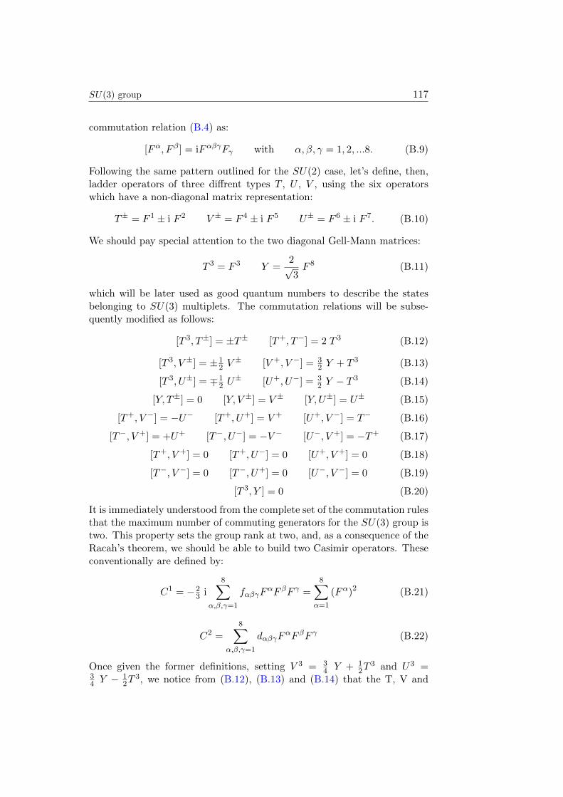
SU(3) group 117
commutation relation (B.4) as:
[Fα, F β] = iFαβγFγ with α, β, γ = 1, 2, ...8. (B.9)
Following the same pattern outlined for the SU(2) case, let’s define, then,ladder operators of three diffrent types T , U , V , using the six operatorswhich have a non-diagonal matrix representation:
T± = F 1 ± i F 2 V ± = F 4 ± i F 5 U± = F 6 ± i F 7. (B.10)
We should pay special attention to the two diagonal Gell-Mann matrices:
T 3 = F 3 Y =2√3F 8 (B.11)
which will be later used as good quantum numbers to describe the statesbelonging to SU(3) multiplets. The commutation relations will be subse-quently modified as follows:
[T 3, T±] = ±T± [T+, T−] = 2 T 3 (B.12)
[T 3, V ±] = ±12 V
± [V +, V −] = 32 Y + T 3 (B.13)
[T 3, U±] = ∓12 U
± [U+, U−] = 32 Y − T 3 (B.14)
[Y, T±] = 0 [Y, V ±] = V ± [Y,U±] = U± (B.15)
[T+, V −] = −U− [T+, U+] = V + [U+, V −] = T− (B.16)
[T−, V +] = +U+ [T−, U−] = −V − [U−, V +] = −T+ (B.17)
[T+, V +] = 0 [T+, U−] = 0 [U+, V +] = 0 (B.18)
[T−, V −] = 0 [T−, U+] = 0 [U−, V −] = 0 (B.19)
[T 3, Y ] = 0 (B.20)
It is immediately understood from the complete set of the commutation rulesthat the maximum number of commuting generators for the SU(3) group istwo. This property sets the group rank at two, and, as a consequence of theRacah’s theorem, we should be able to build two Casimir operators. Theseconventionally are defined by:
C1 = −23 i
8∑α,β,γ=1
fαβγFαF βF γ =
8∑α=1
(Fα)2 (B.21)
C2 =
8∑α,β,γ=1
dαβγFαF βF γ (B.22)
Once given the former definitions, setting V 3 = 34 Y + 1
2T3 and U3 =
34 Y − 1
2T3, we notice from (B.12), (B.13) and (B.14) that the T, V and
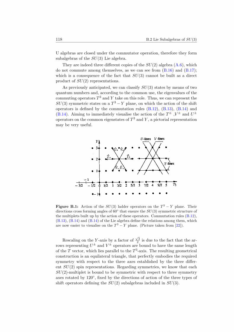
118 B.2 Lie Subalgebras of SU(3)
U algebras are closed under the commutator operation, therefore they formsubalgebras of the SU(3) Lie algebra.
They are indeed three different copies of the SU(2) algebra (A.6), whichdo not commute among themselves, as we can see from (B.16) and (B.17);which is a consequence of the fact that SU(3) cannot be built as a directproduct of SU(2) representations.
As previously anticipated, we can classify SU(3) states by means of twoquantum numbers and, according to the common use, the eigenvalues of thecommuting operators T 3 and Y take on this role. Thus, we can represent theSU(3) symmetric states on a T 3− Y plane, on which the action of the shiftoperators is defined by the commutation rules (B.12), (B.13), (B.14) and(B.14). Aiming to immediately visualise the action of the T± ,V ± and U±
operators on the common eigenstates of T 3 and Y , a pictorial representationmay be very useful.
Figure B.1: Action of the SU(3) ladder operators on the T 3 − Y plane. Theirdirections cross forming angles of 60 that ensure the SU(3) symmetric structure ofthe multiplets built up by the action of these operators. Commutation rules (B.12),(B.13), (B.14) and (B.14) of the Lie algebra define the relations among them, whichare now easier to visualise on the T 3 − Y plane. (Picture taken from [22]).
Rescaling on the Y -axis by a factor of√32 is due to the fact that the ar-
rows representing U± and V ± operators are bound to have the same lengthof the T vector, which lies parallel to the T 3-axis. The resulting geometricalconstruction is an equilateral triangle, that perfectly embodies the requiredsymmetry with respect to the three axes established by the three differ-ent SU(2) spin representations. Regarding symmetries, we know that eachSU(2)-multiplet is bound to be symmetric with respect to three symmetryaxes rotated by 120, fixed by the directions of action of the three types ofshift operators defining the SU(2) subalgebras included in SU(3).
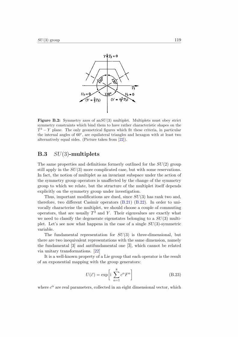
SU(3) group 119
Figure B.2: Symmetry axes of anSU(3) multiplet. Multiplets must obey strictsymmetry constraints which bind them to have rather characteristic shapes on theT 3 − Y plane. The only geometrical figures which fit these criteria, in particularthe internal angles of 60, are equilateral triangles and hexagon with at least twoalternatively equal sides. (Picture taken from [22]).
B.3 SU(3)-multiplets
The same properties and definitions formerly outlined for the SU(2) groupstill apply in the SU(3) more complicated case, but with some reservations.In fact, the notion of multiplet as an invariant subspace under the action ofthe symmetry group operators is unaffected by the change of the symmetrygroup to which we relate, but the structure of the multiplet itself dependsexplicitly on the symmetry group under investigation.
Thus, important modifications are dued, since SU(3) has rank two and,therefore, two different Casimir operators (B.21) (B.22). In order to uni-vocally characterise the multiplet, we should choose a couple of commutingoperators, that are usually T 3 and Y . Their eigenvalues are exactly whatwe need to classify the degenerate eigenstates belonging to a SU(3) multi-plet. Let’s see now what happens in the case of a single SU(3)-symmetricvariable.
The fundamental representation for SU(3) is three-dimensional, butthere are two inequivalent representations with the same dimension, namelythe fundamental [3] and antifundamental one [3], which cannot be relatedvia unitary transformations. [22]
It is a well-known property of a Lie group that each operator is the resultof an exponential mapping with the group generators:
U(~c ) = exp
[i
8∑α=1
cαFα]
(B.23)
where cα are real parameters, collected in an eight dimensional vector, which
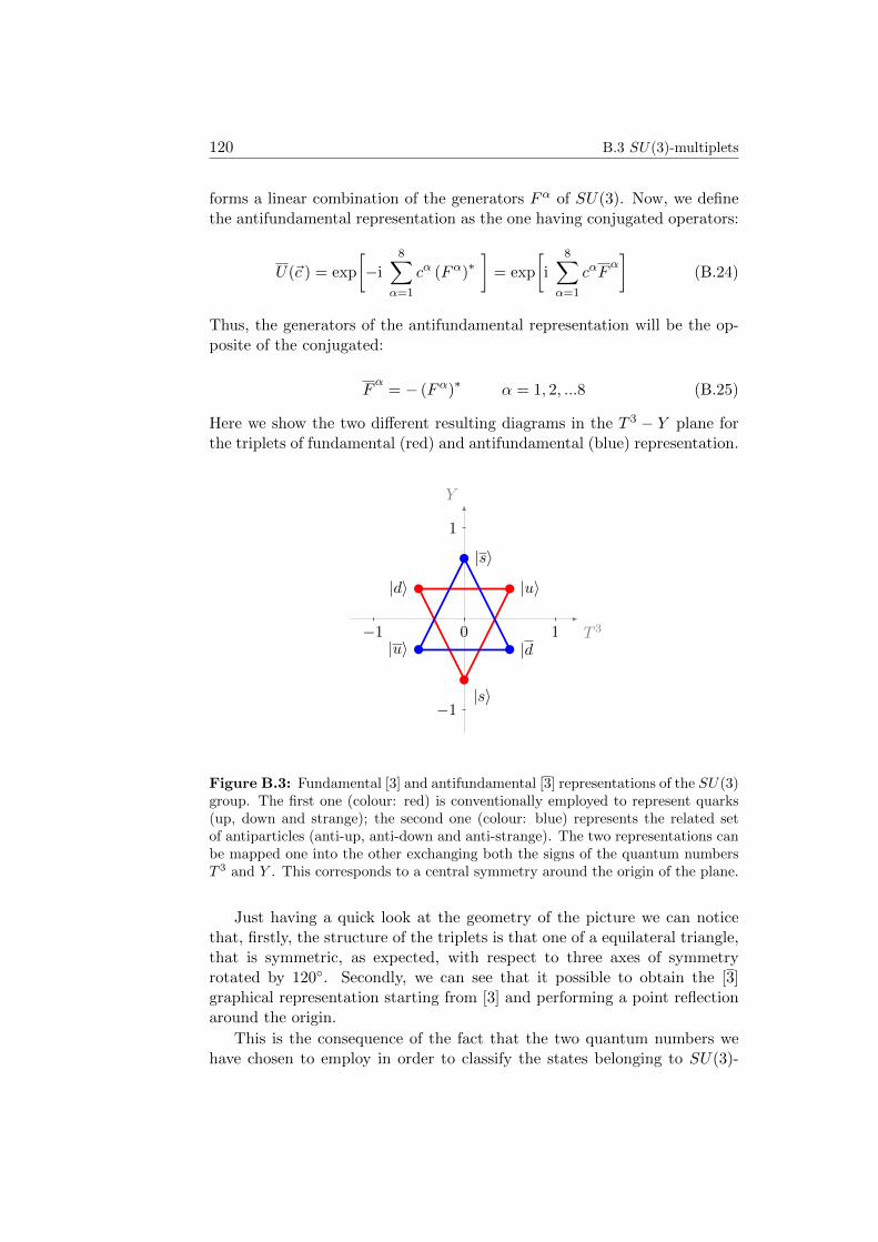
120 B.3 SU(3)-multiplets
forms a linear combination of the generators Fα of SU(3). Now, we definethe antifundamental representation as the one having conjugated operators:
U(~c ) = exp
[−i
8∑α=1
cα (Fα)∗]
= exp
[i
8∑α=1
cαFα]
(B.24)
Thus, the generators of the antifundamental representation will be the op-posite of the conjugated:
Fα
= − (Fα)∗ α = 1, 2, ...8 (B.25)
Here we show the two different resulting diagrams in the T 3 − Y plane forthe triplets of fundamental (red) and antifundamental (blue) representation.
T 3
Y
101
1
1
|ui|di
|si
|ui |d
|si
1
Figure B.3: Fundamental [3] and antifundamental [3] representations of the SU(3)group. The first one (colour: red) is conventionally employed to represent quarks(up, down and strange); the second one (colour: blue) represents the related setof antiparticles (anti-up, anti-down and anti-strange). The two representations canbe mapped one into the other exchanging both the signs of the quantum numbersT 3 and Y . This corresponds to a central symmetry around the origin of the plane.
Just having a quick look at the geometry of the picture we can noticethat, firstly, the structure of the triplets is that one of a equilateral triangle,that is symmetric, as expected, with respect to three axes of symmetryrotated by 120. Secondly, we can see that it possible to obtain the [3]graphical representation starting from [3] and performing a point reflectionaround the origin.
This is the consequence of the fact that the two quantum numbers wehave chosen to employ in order to classify the states belonging to SU(3)-
SU(3) group 121
multiplets are the eigenvalues of the two real operators:
T 3 =1
2
1 0 00 −1 00 0 0
Y =1
3
1 0 00 1 00 0 −2
(B.26)
Their antifundamental is, according to (B.25), the opposite of the conjugatedmatrix operator, resulting in a change of sign for all quantum numbers.
The composite effect of these two axial symmetries with respect to thetwo cartesian axes, gives a central symmetry with the origin as the reflectionpoint.
The states individuated by the vertices of the equilateral triangles havetheir own quantum numbers classifying them as follows:
|u〉 =∣∣T 3 = 1
2 , Y = 13
⟩(B.27)
|d〉 =∣∣T 3 = −1
2 , Y = 13
⟩(B.28)
|s〉 =∣∣T 3 = 0, Y = −2
3
⟩(B.29)
conventionally labelled by the name of quarks -up, down, strange- they arerelated to when we deal with SU(3) as a QCD symmetry group. A similarinterpretation is given to the antifundamental representation states, whichwe may see as the respective antiparticles: anti-up, anti-down and anti-strange.
|u〉 =∣∣T 3 = −1
2 , Y = −13
⟩(B.30)
∣∣d⟩ =∣∣T 3 = 1
2 , Y = −13
⟩(B.31)
|s〉 =∣∣T 3 = 0, Y = 2
3
⟩(B.32)
Higher dimensional multiplets will appear in the operation of composi-tion of representations by means of Kronecker products, that mix the fun-damental and antifundamental types of representations.
Here we will show some of the lowest dimensional irreducible represen-tations of the SU(3) group.
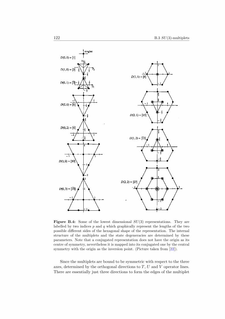
122 B.3 SU(3)-multiplets
Figure B.4: Some of the lowest dimensional SU(3) representations. They arelabelled by two indices p and q which graphically represent the lengths of the twopossible different sides of the hexagonal shape of the representation. The internalstructure of the multiplets and the state degeneracies are determined by theseparameters. Note that a conjugated representation does not have the origin as itscentre of symmetry, nevertheless it is mapped into its conjugated one by the centralsymmetry with the origin as the inversion point. (Picture taken from [22]).
Since the multiplets are bound to be symmetric with respect to the threeaxes, determined by the orthogonal directions to T , U and V operator lines.There are essentially just three directions to form the edges of the multiplet
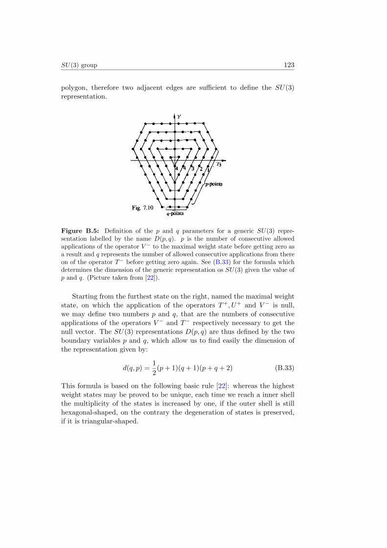
SU(3) group 123
polygon, therefore two adjacent edges are sufficient to define the SU(3)representation.
Figure B.5: Definition of the p and q parameters for a generic SU(3) repre-sentation labelled by the name D(p, q). p is the number of consecutive allowedapplications of the operator V − to the maximal weight state before getting zero asa result and q represents the number of allowed consecutive applications from thereon of the operator T− before getting zero again. See (B.33) for the formula whichdetermines the dimension of the generic representation os SU(3) given the value ofp and q. (Picture taken from [22]).
Starting from the furthest state on the right, named the maximal weightstate, on which the application of the operators T+, U+ and V − is null,we may define two numbers p and q, that are the numbers of consecutiveapplications of the operators V − and T− respectively necessary to get thenull vector. The SU(3) representations D(p, q) are thus defined by the twoboundary variables p and q, which allow us to find easily the dimension ofthe representation given by:
d(q, p) =1
2(p+ 1)(q + 1)(p+ q + 2) (B.33)
This formula is based on the following basic rule [22]: whereas the highestweight states may be proved to be unique, each time we reach a inner shellthe multiplicity of the states is increased by one, if the outer shell is stillhexagonal-shaped, on the contrary the degeneration of states is preserved,if it is triangular-shaped.

Appendix C
Alternative mapping
In this appendix we propose an alternative mapping of the purely biquadraticspin-1 model into a SU(3) Heisenberg chain, which makes it considerablyeasier to prove the equivalence between the two models, but eventually yieldsto a non-diagonal form of the operator T 3
i acting on each site. This furthercomplicates the interpretation of T 3
tot in terms of SU(2) quantum numbers,preventing us from fulfilling our purpose to map the Bethe ansatz classifi-cation of eigenstates in a wider SU(3)-symmetric structure.
C.1 Alternative form of the SU(3)Heisenberg chain
It may be convenient to deal with the SU(3) Heisenberg Hamiltonian ina slightly different formulation from the usual one in terms of Gell-Mannmatrices. We will restrict our analysis to the most relevant case for ourdiscussion, that is:
HF⊗A(±J) = ±JN∑i=1
[ −λ8iλ8i+1 − λ3iλ3i+1+
− λ1iλ1i+1 + λ2iλ2i+1 − λ4iλ4i+1 + λ5iλ
5i+1 − λ6iλ6i+1 + λ7iλ
7i+1 ]
(C.1)
which has alternate fundamental and antifundamental representations onodd and even sites.
Since for the spin-1/2 operators it is possible to express the combinationSxi S
xi+1+Syi S
yi+1 in terms of the SU(2) ladder operators, namely 1
2(S−i S+i+1+
S+i S−i+1), we may attempt to do the same for the spin-1 operators too. In
order to do so, all the ladder operators T±, U± and V ± characterising thethree SU(2) subalgebras included in the SU(3) group have to be employed.
125
126 C.2 Mapping between spin-1 operators and Gell-Mann matrices
By means of definition (B.10) we get to the identity:
T+i T
+i+1 + T−i T
−i+1 =
=1
4(λ1i + iλ2i )(λ
1i+1 + iλ2i+1) +
1
4(λ1i − iλ2i )(λ
1i+1 − iλ2i+1) =
=1
2(λ1iλ
1i+1 − λ2iλ2i+1)
(C.2)
Similarly for the other two cases:
U+i U
+i+1 + U−i U
−i+1 =
1
2(λ6iλ
6i+1 − λ7iλ7i+1) (C.3)
V +i V
+i+1 + V −i V
−i+1 =
1
2(λ4iλ
4i+1 − λ5iλ5i+1) (C.4)
Eventually, the SU(3) Heisenberg Hamiltonian (C.1) can be rewritten in thefollowing form:
HF⊗A(±J) = ∓JN∑i=1
[ T+i T
+i+1 + T−i T
−i+1 + U+
i U+i+1 + U−i U
−i+1+
+ V +i V
+i+1 + V −i V
−i+1 + 2T 3
i T3i+1 +
3
2YiYi+1]
(C.5)
where the last two Gell-Mann matrices λ3 and λ8 have been replaced bytheir related SU(3) operators T 3 and Y (B.11) .
C.2 Mapping between spin-1 operators and Gell-Mann matrices
The following pages outline the complete mapping between the SU(3)-symmetric Heisenberg chain and two special cases of the spin-1 bilinear-biquadratic models, i.e. the pure biquadratic and the Lai-Sutherland mod-els. As previously stated, this mapping [13] is indeed the easiest way toprove the equivalence between the models under investigation. In fact, theequivalence between the two Hamiltonians follows immediately, once the ba-sic equivalence with the generators of SU(2) algebra has been established.Namely:
S1 = λ7 S2 = −λ5 S3 = λ2 (C.6)
Let’s make now, the correspondence with the SU(3) operators for someoperators which turn out to be part of the bilinear-biquadratic model. Firstlythe squares of the spin components:
(S1)2 =1
2
(−λ3 − 1√
3λ8 +
4
3
)(C.7)
Alternative mapping 127
(S2)2 =1
2
(λ3 − 1√
3λ8 +
4
3
)(C.8)
(S3)2 =1
3
(√3λ8 + 2
)(C.9)
and then the mixed products of components:
S1S2 = −1
2
(λ1 − iλ2
)S2S1 = −1
2
(λ1 + iλ2
)(C.10)
S1S3 = −1
2
(λ4 − iλ5
)S3S1 = −1
2
(λ4 + iλ5
)(C.11)
S2S3 = −1
2
(λ6 − iλ7
)S3S2 = −1
2
(λ6 + iλ7
)(C.12)
Let us start with the bilinear form of the SU(2)-symmetric HeisenbergHamiltonian, having the following expression in terms of spin-1 operators:
HHeis(J) = J
N∑i=1
((S1i )(S1
i+1) + (S2i )(S2
i+1) + (S3i )(S3
i+1)
)(C.13)
Using the mapping (C.6), it is easy to see that:
(S1i )(S1
i+1) + (S2i )(S2
i+1) + (S3i )(S3
i+1) = λ7iλ7i+1 + λ5iλ
5i+1 + λ2iλ
2i+1 (C.14)
Now, let’s deal with the biquadratic term of the Hamiltonian, whichyields nine different terms:
HbiQ(−J) = −JN∑i=1
((S1i )2(S1
i+1)2 + (S2
i )2(S2i+1)
2 + (S3i )2(S3
i+1)2+
+ (S1i S
2i )(S1
i+1S2i+1) + (S2
i S1i )(S2
i+1S1i+1) + (S1
i S3i )(S1
i+1S3i+1)+
+ (S3i S
1i )(S3
i+1S1i+1) + (S2
i S3i )(S2
i+1S3i+1) + (S3
i S2i )(S3
i+1S2i+1)
) (C.15)
In order to complete the mapping we need the biquadratic terms and thequadratic mixed products. Using the identities (C.7), (C.8) and (C.9), weget:
(S1i )2(S1
i+1)2 =
1
4
(λ3iλ
3i+1 +
1
3λ8iλ
8i+1 +
16
9+
+1√3λ3iλ
8i+1 +
1√3λ8iλ
3i+1 −
4
3√
3λ8i −
4
3√
3λ8i+1 −
4
3λ3i −
4
3λ3i+1
) (C.16)
(S2i )2(S2
i+1)2 =
1
4
(λ3iλ
3i+1 +
1
3λ8iλ
8i+1 +
16
9+
− 1√3λ3iλ
8i+1 −
1√3λ8iλ
3i+1 −
4
3√
3λ8i −
4
3√
3λ8i+1 +
4
3λ3i +
4
3λ3i+1
) (C.17)
128 C.2 Mapping between spin-1 operators and Gell-Mann matrices
(S3i )2(S3
i+1)2 =
1
3λ8iλ
8i+1 +
4
9+
2
3√
3λ8i +
2
3√
3λ8i+1 (C.18)
Now, using the identities (C.10), (C.11) and (C.12), we may deal with themixed products, for which a convenient cancellation of terms occurs, leadingto the following relations:
(S1i S
2i )(S1
i+1S2i+1) + (S2
i S1i )(S2
i+1S1i+1) =
1
2
(λ1iλ
1i+1 − λ2iλ2i+1
)(C.19)
(S1i S
3i )(S1
i+1S3i+1) + (S3
i S1i )(S3
i+1S1i+1) =
1
2
(λ4iλ
4i+1 − λ5iλ5i+1
)(C.20)
(S2i S
3i )(S2
i+1S3i+1) + (S3
i S2i )(S3
i+1S2i+1) =
1
2
(λ6iλ
6i+1 − λ7iλ7i+1
)(C.21)
Finally, collecting these results all together we may write the most generalform of the bilinear-biquadratic spin-1 Hamiltonian, parametrised by meansof two coefficients α and β. Suitable choices of their values correspond todifferent models represented in the phase space of fig. 1.1.
H(α, β) = αHHeis + βHbiQ =
=N∑i=1
α (λ2iλ2i+1 + λ5iλ
5i+1 + λ7iλ
7i+1)+
+N∑i=1
12β
(λ8iλ
8i+1 + λ3iλ
3i+1 + 8
3+
+ λ1iλ1i+1 − λ2iλ2i+1 + λ4iλ
4i+1 − λ5iλ5i+1 + λ6iλ
6i+1 − λ7iλ7i+1
)(C.22)
In order to recover the pure-biquadratic exchange Hamiltonian we need toselect the value α = 0 in (C.22), which erases the presence of the bilinearinteraction. The resulting expression in terms of standard SU(3) generatorscan be interpreted as a SU(3) Heisenberg chain with alternate fundamentaland antifundamental representations on odd and even sites, which cause thesigns to change in some given products of Gell-Mann matrices.
HbiQ(±J) = H(α = 0, β = ±J) = ±12J
N∑i=1
[ λ8iλ8i+1 + λ3iλ
3i+1+
+ λ1iλ1i+1 − λ2iλ2i+1 + λ4iλ
4i+1 − λ5iλ5i+1 + λ6iλ
6i+1 − λ7iλ7i+1 ]± 4
3JN =
= −12HF⊗A(±J)± 4
3JN
(C.23)
Alternative mapping 129
In order to recover the Lai-Sutherland model, we need the coefficients of thebilinear and biquadratic terms to be equal, thus we may select α = β inequation (C.22) to finally get:
HLS(±J) = H(α = β = ±J)± 12J
N∑i=1
[ λ8iλ8i+1 + λ3iλ
3i+1+
+ λ1iλ1i+1 + λ2iλ
2i+1 + λ4iλ
4i+1 + λ5iλ
5i+1 + λ6iλ
6i+1 + λ7iλ
7i+1 ]± 4
3JN =
= 12HF⊗F (±J)± 4
3JN
(C.24)
which clearly represents a SU(3) Heisenberg model with the same type ofrepresentation on both even and odd sites.

Bibliography
[1] I. Affleck, Exact critical exponents for quantum spin chains, non-linearσ-models at θ = π and the quantum Hall effect, Nucl. Phys. B265, 409-447, (1986).
[2] I. Affleck, Exact results on the dimerisation transition in SU(n) anti-ferromagnetic chains, J. Phys. 2, 405-415, (1990).
[3] I. Affleck, T. Kennedy, E. H. Lieb, H. Tasaki, Rigorous results onvalence-bond ground states in antiferromagnetis, Phys. Rev. Lett. 59,799-802, (1987).
[4] I. Affleck, T. Kennedy, E. H. Lieb, H. Tasaki, Valence bond groundstates in isotropic quantum antiferromagnets, Commun. Math. Phys.115, 477-528, (1988).
[5] F. C. Alcaraz, M. N. Barber, M. T. Batchelor, Conformal invariance,the XXZ chain and the operator content of two-dimensional criticalsystems, Ann. Phys. N.Y. 182, 280-343, (1988).
[6] F. C. Alcaraz, M. N. Barber, M. T. Batchelor, Surface exponents ofthe quantum XXZ, Ashkin-Teller and Potts models, J. Phys. A 20,6397-6409, (1987)
[7] M. Andres, I. Schneider, S. Eggert, Highest weight state description ofthe isotropic spin-1 chain, Phys. Rew. B 77, 014429 1-7, (2008).
[8] H. M. Babujian, Exact solution of the one-dimensional isotropicHeisenberg chain with arbitary spin s, Phys. Lett.90A, 479-482, (1982).
[9] M. N. Barber, M. T. Batchelor, Spectrum of the biquadratic spin-1antiferromagnetic chain, Phys. Rew. B 40, 4621-4626, (1989).
[10] M. N. Barber, M. T. Batchelor, Spin-s quantum chains and Temperly-Lieb algebras, J. Phys. A, L15-L21, (1990).
[11] R. J. Baxter, Exactly solved models in statistical mechanics, AcademicPress, (1982).
131
132 Bibliography
[12] R. J. Baxter, H. N. V. Temperley , S. E. Ashley Triangular PottsModel at its Transition Temperature, and Related Models, Proc. Roy.Soc. London 358A,535-559, (1978).
[13] C. Benassi, SU(3) lattice gauge theories and spin chains,http://amslaurea.unibo.it, (2014).
[14] E. Berkcan, On the order-disorder variables, duality and the functionalinversion relation, Nucl. Phys. B215, 68-82, (1983).
[15] J. C. Bonner, J. B. Parkinson, J. Oitmaa, H. W. J. Blote, Unusual crit-ical behavior in a bilinear-biquadratic exchange Hamiltonian, J. Appl.Phys. 61, 4432-4434, (1987).
[16] J. Des Cloizeaux, M. Gaudin, H. W. J. Blote, Anisotropic LinearMagnetic Chain, J. Math. Phys. 7, 1384-1400 (1966).
[17] K. Chang, I. Affleck, G. W. Hayden, Z. G. Soos, A study of the bilinear-biqudratic spin-1 antiferromagnetic chain using the valence-bond basis,J. Phys. 1, 153-167, (1989).
[18] P. Di Francesco, P. Mathieu, D. Senechal, Conformal field theory,Springer, (1997).
[19] G. Fath, J. Solyom, Isotropic spin-1 chain with twisted boundary con-dition, Phys. Rev. B 47 , 872-881, (1993).
[20] G. Fath, J. Solyom, Solitonic excitations in the Haldane phase of anS=1 chain , J. Phys. 5, 8983-8998, (1993).
[21] G. Fath, J. Solyom, Search for the nondimerized quantum nematicphase in the spin-1 chain, Phys. Rev. B 51, 3620-3625, (1995).
[22] W. Greiner, B. Muller, Quantum mechanics symmetries, Springer,(1994).
[23] F. D. M. Haldane, Continuum dynamics of the 1-D Heisenberg antifer-romagnet: identification with the O(3) nonlinear sigma model, Phys.Lett. 93A, 463-468, (1983).
[24] F. D. M. Haldane, Nonlinear Field Theory of Large-Spin Heisen-berg Antiferromagnets: Semiclassically Quantized Solitons of the One-Dimensional Easy-Axis Neel State, Phys. Rev. Lett. 50, 1153-1156,(1983).
[25] M. Henkel, Conformal invariance and critical phenomena, Springer,(1999).
Bibliography 133
[26] T. Kennedy, H.Tasaki, Hidden symmetry breaking and the Haldanephase in S=1 quantum spin chains, Commun. Math. Phys. 147, 431-484, (1992).
[27] A. Klumper, The spectra of q-state vertex models and related antifer-romagnetic quantum spin chain, J. Phys. A23, 809-823, (1989).
[28] A. Klumper, New results for q-state vertex models and pure biquadraticspin-1 Hamiltonian, Europhys. Lett.9, 815-820, (1989).
[29] C. K. Lai, Lattice gas with nearest neighbor interaction in one dimen-sion with arbitrary statistics, J. Math. Phys. 15, 1675-1676, (1974).
[30] M. P. Nightingale, H. J. Blote, Gap of the linear spin-1 Heisenbergantiferromagnet: a Monte Carlo calculation, Phys. Rev B 33, 659-661,(1986).
[31] J. B. Parkinson, The S = 1 quantum spin chain with pure biquadraticexchange, J.Phys. C 20, L1029-L1032, (1987).
[32] J. B. Parkinson, The S = 1 quantum spin chain with pure biquadraticexchange, J.Phys. C 21, 3793-3806, (1988).
[33] J. H. H. Perk, C. L. Schultz, Families of commuting transfer matricesin q-state vertex models, Yang-Baxter equation in integrable systems,Michio Jimbo, (1989).
[34] J. H. H. Perk, F. Y. Wu, Nonintersecting String Model and GraphicalApproach: Equivalence with a Ports Model, J. Stat. Phys. 42, 727-742,(1986).
[35] U. Schollwock, Th. Jolicoeur, T. Garel, Onset of incommensurabilityat the valence-bond-solid point in the S=1 quantum spin chain, Phys.Rew. B 53, 3304-3311, (1995).
[36] J. Solyom, Competing bilinear and biquadratic exchange couplings inspin-1 Heisenberg chains, Phys. B 36, 8642-8648, (1987).
[37] J. Solyom, P. Pfeuty, Renormalization-group study of Hamiltonian ver-sion of the Potts model, Phys. Rew. B 24, 147, 218-229, (1981).
[38] Yu. G. Stroganov, A new calculation method for partition functions insome lattice models, Phys. Lett. 74A, 116-118, (1979).
[39] B. Sutherland, Model for a multicomponent quantum system, Phys.Rev. B 12 , 3795-3805, (1975).
[40] M. Takahashi, Thermodynamics of one-dimensional solvable models,Cambridge University Press, (1999).
134 Bibliography
[41] L. A. Takhtajan, The picture of low-lying excitations in the isotropicHeisenberg chain of arbitrary spin, Phys. Lett. 87A, 479-482, (1982).