ANALYSIS OF THE ROTATIONAL PROPERTIES OF KUIPER BELT

ANALYSIS OF THE ROTATIONAL PROPERTIES OF KUIPER BELT OBJECTS

Pedro Lacerda1, 2

Grupo de Astrof ısica da Universidade de Coimbra, Departamento de Matematica, Largo D. Dinis, 3000 Coimbra, Portugal;

[email protected]

and

Jane Luu

Lincoln Laboratory, Massachusetts Institute of Technology, 244 Wood Street, Lexington, MA 02420

Received 2005 October 4; accepted 2006 January 6

ABSTRACT

We use optical data on 10 Kuiper Belt objects (KBOs) to investigate their rotational properties. Of the 10, 3 (30%)exhibit light variations with amplitude �m � 0:15 mag, and 1 out of 10 (10%) has �m � 0:40 mag, which is ingood agreement with previous surveys. These data, in combination with the existing database, are used to discuss therotational periods, shapes, and densities of KBOs. We find that, in the sampled size range, KBOs have a higher frac-tion of low-amplitude light curves and rotate slower than main-belt asteroids. The data also show that the rotationalproperties and the shapes of KBOs depend on size. If we split the database of KBO rotational properties into two sizeranges with diameters larger and smaller than 400 km, we find that (1) the mean light-curve amplitudes of the twogroups are different with 98.5% confidence, (2) the corresponding power-law shape distributions seem to be different,although the existing data are too sparse to render this difference significant, and (3) the two groups occupy differentregions on a spin period–versus–light-curve amplitude diagram. These differences are interpreted in the context ofKBO collisional evolution.

Key words: Kuiper Belt — minor planets, asteroids — solar system: general

1. INTRODUCTION

The Kuiper Belt (KB) is an assembly of mostly small icyobjects, orbiting the Sun beyond Neptune. Kuiper Belt objects(KBOs) are likely remnants of outer solar system planetesimals(Jewitt & Luu 1993). Their physical, chemical, and dynamicalproperties should therefore provide valuable information regard-ing both the environment and the physical processes responsiblefor planet formation.

At the time of writing, roughly 1000 KBOs are known, halfof which have been followed for more than one opposition. A to-tal of �105 objects larger than 50 km are thought to orbit theSun beyond Neptune (Jewitt & Luu 2000). Studies of KB orbitshave revealed an intricate dynamical structure, with signatures ofinteractions with Neptune (Malhotra 1995). The size distribu-tion follows a differential power law of index q ¼ 4 for bodiesk50 km (Trujillo et al. 2001a), becoming slightly shallower atsmaller sizes (Bernstein et al. 2004).

KBO colors show a large diversity, from slightly blue to veryred (Luu & Jewitt 1996; Tegler & Romanishin 2000; Jewitt &Luu 2001), and seem to correlate with inclination and/or perihe-lion distance (e.g., Jewitt & Luu 2001; Doressoundiram et al.2002; Trujillo & Brown 2002). The few low-resolution opticaland near-IR KBO spectra are mostly featureless, with the excep-tion of a weak 2 �mwater ice absorption line present in some ofthem (Brown et al. 1999; Jewitt & Luu 2001) and strong meth-ane absorption on 2003 UB313 (Brown et al. 2005).

About 4% of known KBOs are binaries with separationslarger than 0B15 (Noll et al. 2002). All the observed binarieshave primary-to-secondary mass ratios�1. Two binary creation

models have been proposed. Weidenschilling (2002) favors theidea that binaries form in three-body encounters. This model re-quires a 100 times more dense Kuiper Belt at the epoch of binaryformation and predicts a higher abundance of large-separationbinaries. An alternative scenario (Goldreich et al. 2002), in whichthe energy needed to bind the orbits of two approaching bodiesis drawn from the surrounding swarm of smaller objects, also re-quires a much higher density of KBOs than the present, but it pre-dicts a larger fraction of close binaries. Recently, Sheppard &Jewitt (2004) have shown evidence that 2001 QG298 could be aclose or contact binary KBO and estimated the fraction of similarobjects in the Belt to be �10%–20%.Other physical properties of KBOs, such as their shapes, den-

sities, and albedos, are still poorly constrained. This is mainlybecause KBOs are extremely faint, with mean apparent red mag-nitude mR � 23 (Trujillo et al. 2001b).The study of KBO rotational properties through time-series

broadband optical photometry has proved to be the most suc-cessful technique to date for investigating some of these physicalproperties. Light variations of KBOs are believed to be causedmainly by their aspherical shape; as KBOs rotate in space, theirprojected cross sections change, resulting in periodic brightnessvariations.One of the best examples to date of a KBO light curve—and

what can be learned from it—is that of (20000) Varuna (Jewitt &Sheppard 2002). The authors explained the light curve of (20000)Varuna as a consequence of its elongated shape (axis ratio, a/b �1:5). They further argued that the object is centripetally deformedby rotation because of its low-density ‘‘rubble pile’’ structure. Theterm ‘‘rubble pile’’ is generally used to refer to gravitationallybound aggregates of smaller fragments. The existence of rubblepiles is thought to be due to continuingmutual collisions through-out the age of the solar system, which gradually fracture theinteriors of objects. Rotating rubble piles can adjust their shapes

1 Institute for Astronomy, University of Hawaii, 2680 Woodlawn Drive,Honolulu, HI 96822.

2 Leiden Observatory, Postbus 9513, NL-2300 RA, Leiden, Netherlands.

2314

The Astronomical Journal, 131:2314–2326, 2006 April

# 2006. The American Astronomical Society. All rights reserved. Printed in U.S.A.

to balance centripetal acceleration and self-gravity. The result-ing equilibrium shapes have been studied in the extreme caseof fluid bodies and depend on the body’s density and spin rate(Chandrasekhar 1969).

Lacerda & Luu (2003, hereafter LL03a) showed that underreasonable assumptions the fraction ofKBOswith detectable lightcurves can be used to constrain the shape distribution of theseobjects. A follow-up (Luu & Lacerda 2003, hereafter LL03b) onthis work, using a database of light-curve properties of 33 KBOs(Sheppard & Jewitt 2002 [hereafter SJ02], 2003), showed thatalthough most Kuiper Belt objects (�85%) have shapes thatare close to spherical (a/b �1:5), there is a significant fraction(�12%) with highly aspherical shapes (a/b �1:7).

In this paper we use optical data on 10 KBOs to investigate theamplitudes and periods of their light curves. These data are usedin combination with the existing database to investigate the dis-tributions of KBO spin periods and shapes. We discuss theirimplications for the inner structure and collisional evolution ofobjects in the Kuiper Belt.

2. OBSERVATIONS AND PHOTOMETRY

We collected time-series optical data on 10 KBOs at the IsaacNewton 2.5 m (INT) and William Herschel 4 m (WHT) tele-scopes. The INT Wide Field Camera (WFC) is a mosaic of fourEEV 2048 ; 4096 CCDs, each with a pixel scale of 0B33 pixel�1

and spanning approximately 11A3 ; 22A5 in the plane of the sky.The targets are imaged through a Johnson R filter. The WHT

prime focus camera consists of two EEV 2048 ; 4096 CCDswith a pixel scale of 0B24 pixel�1 and covers a sky-projectedarea of 2 ; 8A2 ; 16A4.With this camera we used a Harris R filter.The seeing for the whole set of observations ranged from 1B0 to1B9 FWHM.We tracked both telescopes at sidereal rate and keptintegration times for each object sufficiently short to avoid errorsin the photometry due to trailing effects (see Table 1). No light-travel time corrections have been made.

We reduced the data using standard techniques. The sky back-ground in the flat-fielded images shows variations of less than1% across the chip. Background variations between consecutivenights were less than 5% for most of the data. Cosmic rays wereremoved with the package LA-Cosmic (van Dokkum 2001).

We performed aperture photometry on all objects in the fieldusing the SExtractor software package (Bertin &Arnouts 1996).This software performs circular aperture measurements on eachobject in a frame and puts out a catalog of both the magnitudesand the associated errors. Below we describe how we obtained abetter estimate of the errors.We used apertures ranging from1.5 to2.0 times the FWHM for each frame and selected the aperture thatmaximized the ratio of signal-to-noise. An extra aperture of fiveFWHMs was used to look for possible seeing-dependent trendsin our photometry. The catalogs were matched by selecting onlythe sources that are present in all frames. The slow movement ofKBOs from night to night allows us to successfully match a largenumber of sources in consecutive nights. We discarded all satu-rated sources, as well as those identified to be galaxies.

TABLE 1

Observing Conditions and Geometry

Object Obs. Datea Telescope

Seeingb

(arcsec)

Mvt. Ratec

(arcsec hr�1)

Int. Timed

(s) R.A. Decl.

R e

(AU)

�f

(AU)

� g

(deg)

(19308) 1996 TO66 .............. 1999 Oct 1 WHT 1.8 2.89 500 23 59 46 +03 36 42 45.950 44.958 0.1594

1996 TS66............................. 1999 Sep 30 WHT 1.3 2.62 400, 600 02 26 06 +21 41 03 38.778 37.957 0.8619

1996 TS66............................. 1999 Oct 1 WHT 1.1 2.67 600 02 26 02 +21 40 50 38.778 37.948 0.8436

1996 TS66............................. 1999 Oct 2 WHT 1.5 2.70 600, 900 02 25 58 +21 40 35 38.778 37.939 0.8225

(35671) 1998 SN165............. 1999 Sep 29 WHT 1.5 3.24 360, 400 23 32 46 �01 18 15 38.202 37.226 0.3341

(35671) 1998 SN165............. 1999 Sep 30 WHT 1.4 3.22 360 23 32 41 �01 18 47 38.202 37.230 0.3594

(19521) Chaos...................... 1999 Oct 1 WHT 1.0 1.75 360, 400, 600 03 44 37 +21 30 58 42.399 41.766 1.0616

(19521) Chaos...................... 1999 Oct 2 WHT 1.5 1.79 400, 600 03 44 34 +21 30 54 42.399 41.755 1.0484

(79983) 1999 DF9................ 2001 Feb 13 WHT 1.7 3.19 900 10 27 04 +09 45 16 39.782 38.818 0.3124

(79983) 1999 DF9................ 2001 Feb 14 WHT 1.6 3.21 900 10 26 50 +09 46 25 39.783 38.808 0.2436

(79983) 1999 DF9................ 2001 Feb 15 WHT 1.4 3.22 900 10 26 46 +09 46 50 39.783 38.806 0.2183

(80806) 2000 CM105............ 2001 Feb 11 WHT 1.5 3.14 600, 900 09 18 48 +19 41 59 41.753 40.774 0.1687

(80806) 2000 CM105............ 2001 Feb 13 WHT 1.4 3.12 900 09 18 39 +19 42 40 41.753 40.778 0.2084

(80806) 2000 CM105............ 2001 Feb 14 WHT 1.5 3.11 900 09 18 34 +19 43 02 41.753 40.781 0.2303

(66652) 1999 RZ253............. 2001 Sep 11 INT 1.9 2.86 600 22 02 57 �12 31 06 40.963 40.021 0.4959

(66652) 1999 RZ253............. 2001 Sep 12 INT 1.4 2.84 600 22 02 53 �12 31 26 40.963 40.026 0.5156

(66652) 1999 RZ253............. 2001 Sep 13 INT 1.8 2.82 600 22 02 49 �12 31 49 40.963 40.033 0.5381

(47171) 1999 TC36 .............. 2001 Sep 11 INT 1.9 3.85 600 00 16 49 �07 34 59 31.416 30.440 0.4605

(47171) 1999 TC36 .............. 2001 Sep 12 INT 1.4 3.86 900 00 16 45 �07 35 33 31.416 30.437 0.4359

(47171) 1999 TC36 .............. 2001 Sep 13 INT 1.8 3.88 900 00 16 39 �07 36 13 31.416 30.434 0.4122

(38628) Huya....................... 2001 Feb 28 INT 1.5 2.91 600 13 31 13 �00 39 04 29.769 29.021 1.2725

(38628) Huya....................... 2001 Mar 1 INT 1.8 2.97 360 13 31 09 �00 38 23 29.768 29.009 1.2479

(38628) Huya....................... 2001 Mar 3 INT 1.5 3.08 360 13 31 01 �00 36 59 29.767 28.987 1.1976

2001 CZ31 ............................ 2001 Mar 1 INT 1.3 2.72 600, 900 09 00 03 +16 29 23 41.394 40.522 0.6525

2001 CZ31 ............................ 2001 Mar 3 INT 1.4 2.65 600, 900 08 59 54 +16 30 04 41.394 40.539 0.6954

Note.—Units of right ascension are hours, minutes, and seconds, and units of declination are degrees, arcminutes, and arcseconds.a UT date of observation.b Average seeing of the data.c Average rate of motion of KBO.d Integration times used.e KBO-Sun distance.f KBO-Earth distance.g Phase angle (Sun-object-Earth angle) of observation.

ANALYSIS OF ROTATIONAL PROPERTIES OF KBOs 2315

The KBO light curves were obtained from differential pho-tometry with respect to the brightest nonvariable field stars. Anaverage of the magnitudes of the brightest stars (the referencestars) provides a reference for differential photometry in eachframe. This method allows for small-amplitude brightness varia-tions to be detected even under nonphotometric conditions.

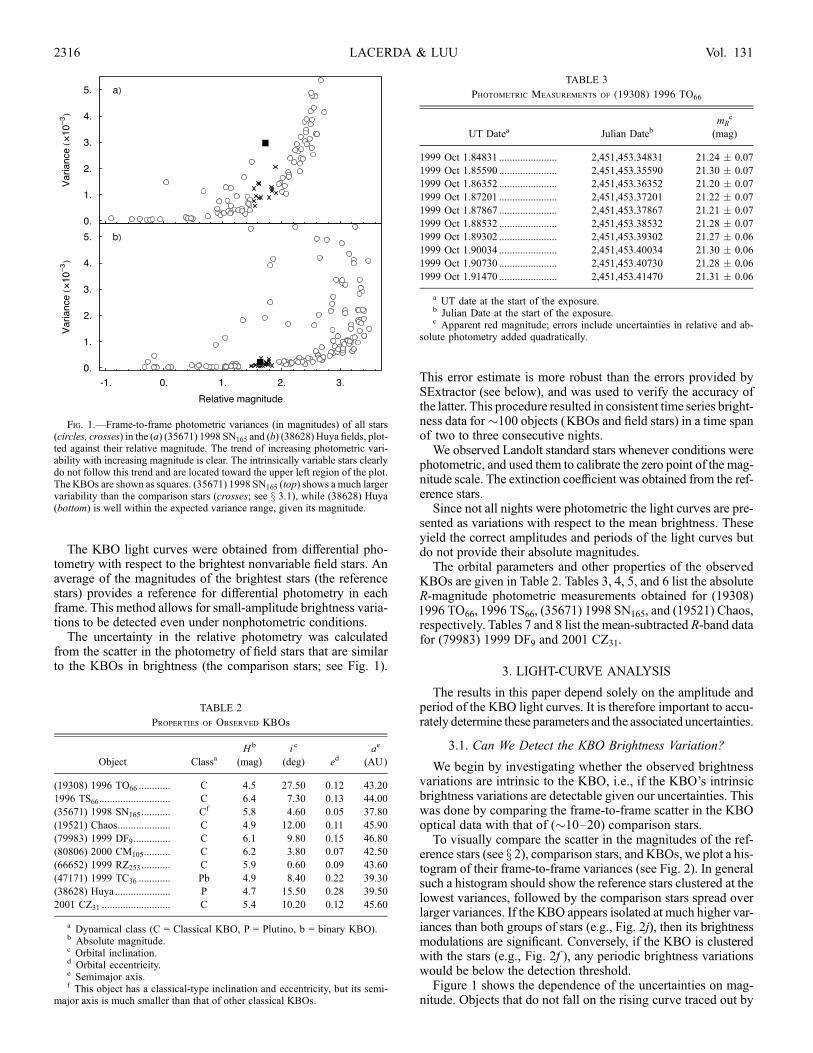
The uncertainty in the relative photometry was calculatedfrom the scatter in the photometry of field stars that are similarto the KBOs in brightness (the comparison stars; see Fig. 1).

This error estimate is more robust than the errors provided bySExtractor (see below), and was used to verify the accuracy ofthe latter. This procedure resulted in consistent time series bright-ness data for�100 objects (KBOs and field stars) in a time spanof two to three consecutive nights.We observed Landolt standard stars whenever conditions were

photometric, and used them to calibrate the zero point of the mag-nitude scale. The extinction coefficient was obtained from the ref-erence stars.Since not all nights were photometric the light curves are pre-

sented as variations with respect to the mean brightness. Theseyield the correct amplitudes and periods of the light curves butdo not provide their absolute magnitudes.The orbital parameters and other properties of the observed

KBOs are given in Table 2. Tables 3, 4, 5, and 6 list the absoluteR-magnitude photometric measurements obtained for (19308)1996 TO66, 1996 TS66, (35671) 1998 SN165, and (19521) Chaos,respectively. Tables 7 and 8 list the mean-subtracted R-band datafor (79983) 1999 DF9 and 2001 CZ31.

3. LIGHT-CURVE ANALYSIS

The results in this paper depend solely on the amplitude andperiod of the KBO light curves. It is therefore important to accu-rately determine these parameters and the associated uncertainties.

3.1. Can We Detect the KBO Brightness Variation?

We begin by investigating whether the observed brightnessvariations are intrinsic to the KBO, i.e., if the KBO’s intrinsicbrightness variations are detectable given our uncertainties. Thiswas done by comparing the frame-to-frame scatter in the KBOoptical data with that of (�10–20) comparison stars.To visually compare the scatter in the magnitudes of the ref-

erence stars (see x 2), comparison stars, and KBOs, we plot a his-togram of their frame-to-frame variances (see Fig. 2). In generalsuch a histogram should show the reference stars clustered at thelowest variances, followed by the comparison stars spread overlarger variances. If the KBO appears isolated at much higher var-iances than both groups of stars (e.g., Fig. 2j), then its brightnessmodulations are significant. Conversely, if the KBO is clusteredwith the stars (e.g., Fig. 2f ), any periodic brightness variationswould be below the detection threshold.Figure 1 shows the dependence of the uncertainties on mag-

nitude. Objects that do not fall on the rising curve traced out by

Fig. 1.—Frame-to-frame photometric variances (in magnitudes) of all stars(circles, crosses) in the (a) (35671) 1998 SN165 and (b) (38628) Huya fields, plot-ted against their relative magnitude. The trend of increasing photometric vari-ability with increasing magnitude is clear. The intrinsically variable stars clearlydo not follow this trend and are located toward the upper left region of the plot.The KBOs are shown as squares. (35671) 1998 SN165 (top) shows a much largervariability than the comparison stars (crosses; see x 3.1), while (38628) Huya(bottom) is well within the expected variance range, given its magnitude.

TABLE 2

Properties of Observed KBOs

Object ClassaH b

(mag)

i c

(deg) edae

(AU)

(19308) 1996 TO66 ............ C 4.5 27.50 0.12 43.20

1996 TS66........................... C 6.4 7.30 0.13 44.00

(35671) 1998 SN165........... Cf 5.8 4.60 0.05 37.80

(19521) Chaos.................... C 4.9 12.00 0.11 45.90

(79983) 1999 DF9.............. C 6.1 9.80 0.15 46.80

(80806) 2000 CM105.......... C 6.2 3.80 0.07 42.50

(66652) 1999 RZ253........... C 5.9 0.60 0.09 43.60

(47171) 1999 TC36 ............ Pb 4.9 8.40 0.22 39.30

(38628) Huya..................... P 4.7 15.50 0.28 39.50

2001 CZ31 .......................... C 5.4 10.20 0.12 45.60

a Dynamical class (C = Classical KBO, P = Plutino, b = binary KBO).b Absolute magnitude.c Orbital inclination.d Orbital eccentricity.e Semimajor axis.f This object has a classical-type inclination and eccentricity, but its semi-

major axis is much smaller than that of other classical KBOs.

TABLE 3

Photometric Measurements of (19308) 1996 TO66

UT Datea Julian DatebmR

c

(mag)

1999 Oct 1.84831 ...................... 2,451,453.34831 21.24 � 0.07

1999 Oct 1.85590 ...................... 2,451,453.35590 21.30 � 0.07

1999 Oct 1.86352 ...................... 2,451,453.36352 21.20 � 0.07

1999 Oct 1.87201 ...................... 2,451,453.37201 21.22 � 0.07

1999 Oct 1.87867 ...................... 2,451,453.37867 21.21 � 0.07

1999 Oct 1.88532 ...................... 2,451,453.38532 21.28 � 0.07

1999 Oct 1.89302 ...................... 2,451,453.39302 21.27 � 0.06

1999 Oct 1.90034 ...................... 2,451,453.40034 21.30 � 0.06

1999 Oct 1.90730 ...................... 2,451,453.40730 21.28 � 0.06

1999 Oct 1.91470 ...................... 2,451,453.41470 21.31 � 0.06

a UT date at the start of the exposure.b Julian Date at the start of the exposure.c Apparent red magnitude; errors include uncertainties in relative and ab-

solute photometry added quadratically.

LACERDA & LUU2316 Vol. 131

the stars must have intrinsic brightness variations. By calculatingthe mean and spread of the variance for the comparison stars(crosses) we can calculate our photometric uncertainties andthus determine whether the KBO brightness variations are sig-nificant (�3 �).

3.2. Period Determination

In the cases inwhich significant brightness variations (see x 3.1)were detected in the light curves, the phase dispersion minimi-zation method was used (PDM; Stellingwerf 1978) to look forperiodicities in the data. For each test period, PDM computes astatistical parameter � that compares the spread of data points inphase bins with the overall spread of the data. The period that bestfits the data is the one that minimizes �. The advantages of PDMare that it is nonparametric, i.e., it does not assume a shape for thelight curve, and it can handle unevenly spaced data. Each data setwas tested for periods ranging from 2 to 24 hr, in steps of 0.01 hr.To assess the uniqueness of the PDM solution, we generated 100Monte Carlo realizations of each light curve, keeping the originaldata times and randomizing the magnitudes within the error bars.We ran PDM on each generated data set to obtain a distribution ofbest-fit periods.

3.3. Amplitude Determination

We used a Monte Carlo experiment to determine the ampli-tude of the light curves for which a period was found. We gener-ated several artificial data sets by randomizing each point withinthe error bar. Each artificial data set was fitted with a Fourierseries, using the best-fit period, and the mode and central 68% of

TABLE 4

Photometric Measurements of 1996 TS66


c

(mag)

1999 Sep 30.06087..................... 2,451,451.56087 21.94 � 0.07

1999 Sep 30.06628..................... 2,451,451.56628 21.83 � 0.07

1999 Sep 30.07979..................... 2,451,451.57979 21.76 � 0.07

1999 Sep 30.08529..................... 2,451,451.58529 21.71 � 0.07

1999 Sep 30.09068..................... 2,451,451.59068 21.75 � 0.07

1999 Sep 30.09695..................... 2,451,451.59695 21.67 � 0.07

1999 Sep 30.01250..................... 2,451,451.60250 21.77 � 0.07

1999 Sep 30.10936..................... 2,451,451.60936 21.76 � 0.06

1999 Sep 30.11705 ..................... 2,451,451.61705 21.80 � 0.06

1999 Sep 30.12486..................... 2,451,451.62486 21.77 � 0.06

1999 Sep 30.13798..................... 2,451,451.63798 21.82 � 0.07

1999 Sep 30.14722..................... 2,451,451.64722 21.74 � 0.06

1999 Sep 30.15524..................... 2,451,451.65524 21.72 � 0.06

1999 Sep 30.16834..................... 2,451,451.66834 21.72 � 0.08

1999 Sep 30.17680..................... 2,451,451.67680 21.83 � 0.07

1999 Sep 30.18548..................... 2,451,451.68548 21.80 � 0.06

1999 Sep 30.19429..................... 2,451,451.69429 21.74 � 0.07

1999 Sep 30.20212..................... 2,451,451.70212 21.78 � 0.07

1999 Sep 30.21010..................... 2,451,451.71010 21.72 � 0.07

1999 Sep 30.21806..................... 2,451,451.71806 21.76 � 0.09

1999 Sep 30.23528..................... 2,451,451.73528 21.73 � 0.07

1999 Sep 30.24355..................... 2,451,451.74355 21.74 � 0.08

1999 Oct 1.02002 ....................... 2,451,452.52002 21.81 � 0.06

1999 Oct 1.02799 ....................... 2,451,452.52799 21.82 � 0.06

1999 Oct 1.03648 ....................... 2,451,452.53648 21.81 � 0.06

1999 Oct 1.04422 ....................... 2,451,452.54422 21.80 � 0.06

1999 Oct 1.93113 ....................... 2,451,453.43113 21.71 � 0.06

1999 Oct 1.94168 ....................... 2,451,453.44168 21.68 � 0.06

1999 Oct 1.95331 ....................... 2,451,453.45331 21.73 � 0.06

1999 Oct 1.97903 ....................... 2,451,453.47903 21.69 � 0.06

1999 Oct 1.99177 ....................... 2,451,453.49177 21.74 � 0.06

1999 Oct 2.00393 ....................... 2,451,453.50393 21.73 � 0.05

1999 Oct 2.01588 ....................... 2,451,453.51588 21.78 � 0.05

1999 Oct 2.02734 ....................... 2,451,453.52734 21.71 � 0.05



TABLE 5

Photometric Measurements of (35671) 1998 SN165


c

(mag)

1999 Sep 29.87384..................... 2,451,451.37384 21.20 � 0.06

1999 Sep 29.88050..................... 2,451,451.38050 21.19 � 0.05

1999 Sep 29.88845..................... 2,451,451.38845 21.18 � 0.05

1999 Sep 29.89811 ..................... 2,451,451.39811 21.17 � 0.05

1999 Sep 29.90496..................... 2,451,451.40496 21.21 � 0.05

1999 Sep 29.91060..................... 2,451,451.41060 21.24 � 0.05

1999 Sep 29.91608..................... 2,451,451.41608 21.18 � 0.05

1999 Sep 29.92439..................... 2,451,451.42439 21.25 � 0.05

1999 Sep 29.93055..................... 2,451,451.43055 21.24 � 0.05

1999 Sep 29.93712..................... 2,451,451.43712 21.26 � 0.06

1999 Sep 29.94283..................... 2,451,451.44283 21.25 � 0.06

1999 Sep 29.94821..................... 2,451,451.44821 21.28 � 0.06

1999 Sep 29.96009..................... 2,451,451.46009 21.25 � 0.06

1999 Sep 29.96640..................... 2,451,451.46640 21.21 � 0.06

1999 Sep 29.97313..................... 2,451,451.47313 21.17 � 0.05

1999 Sep 29.97850..................... 2,451,451.47850 21.14 � 0.05

1999 Sep 29.98373..................... 2,451,451.48373 21.12 � 0.06

1999 Sep 29.98897..................... 2,451,451.48897 21.15 � 0.06

1999 Sep 29.99469..................... 2,451,451.49469 21.15 � 0.06

1999 Sep 29.99997..................... 2,451,451.49997 21.16 � 0.06

1999 Sep 30.00521..................... 2,451,451.50521 21.12 � 0.06

1999 Sep 30.01144 ..................... 2,451,451.51144 21.09 � 0.06

1999 Sep 30.02164..................... 2,451,451.52164 21.18 � 0.06

1999 Sep 30.02692..................... 2,451,451.52692 21.17 � 0.06

1999 Sep 30.84539..................... 2,451,452.34539 21.32 � 0.06

1999 Sep 30.85033..................... 2,451,452.35033 21.30 � 0.06

1999 Sep 30.85531..................... 2,451,452.35531 21.28 � 0.06

1999 Sep 30.86029..................... 2,451,452.36029 21.31 � 0.06

1999 Sep 30.86550..................... 2,451,452.36550 21.21 � 0.06

1999 Sep 30.87098..................... 2,451,452.37098 21.26 � 0.06

1999 Sep 30.87627..................... 2,451,452.37627 21.28 � 0.06

1999 Sep 30.89202..................... 2,451,452.39202 21.23 � 0.05

1999 Sep 30.89698..................... 2,451,452.39698 21.30 � 0.06

1999 Sep 30.90608..................... 2,451,452.40608 21.20 � 0.05

1999 Sep 30.91191 ..................... 2,451,452.41191 21.26 � 0.05

1999 Sep 30.92029..................... 2,451,452.42029 21.15 � 0.05

1999 Sep 30.92601..................... 2,451,452.42601 21.19 � 0.05

1999 Sep 30.93110 ..................... 2,451,452.43110 21.14 � 0.05

1999 Sep 30.93627..................... 2,451,452.43627 21.16 � 0.05

1999 Sep 30.94858..................... 2,451,452.44858 21.18 � 0.05

1999 Sep 30.95363..................... 2,451,452.45363 21.16 � 0.05

1999 Sep 30.95852..................... 2,451,452.45852 21.13 � 0.05

1999 Sep 30.96347..................... 2,451,452.46347 21.17 � 0.05

1999 Sep 30.96850..................... 2,451,452.46850 21.16 � 0.05

1999 Sep 30.97422..................... 2,451,452.47422 21.18 � 0.05

1999 Sep 30.98431..................... 2,451,452.48431 21.18 � 0.05

1999 Sep 30.98923..................... 2,451,452.48923 21.17 � 0.06

1999 Sep 30.99444..................... 2,451,452.49444 21.16 � 0.05

1999 Sep 30.99934..................... 2,451,452.49934 21.20 � 0.05

1999 Oct 1.00424 ....................... 2,451,452.50424 21.16 � 0.05

1999 Oct 1.00992 ....................... 2,451,452.50992 21.18 � 0.06



ANALYSIS OF ROTATIONAL PROPERTIES OF KBOs 2317No. 4, 2006

the distribution of amplitudes were taken as the light-curve am-plitude and 1 � uncertainty, respectively. For the null light curves,i.e., those in which no significant variation was detected, we sub-tracted the typical error bar size from the total amplitude of thedata to obtain an upper limit to the amplitude of the KBO photo-metric variation.

4. RESULTS

In this section we present the results of the light-curve analysisfor each of the observed KBOs. We found significant brightnessvariations (�m > 0:15 mag) for 3 out of 10 KBOs (30%), and�m � 0:40 mag for 1 out of 10 (10%). This is consistent withpreviously published results: SJ02 found a fraction of 31% with�m > 0:15 mag and 23% with �m > 0:40 mag, both consis-tent with our results. The other seven KBOs do not show detect-able variations. The results are summarized in Table 9.

4.1. 1998 SN165

Thebrightness of (35671) 1998SN165 varies significantly ( >5�)more than that of the comparison stars (see Figs. 1 and 2c). Theperiodogram for this KBO shows a very broad minimum aroundP ¼ 9 hr (Fig. 3a). The degeneracy implied by the broad mini-

mumwould only be resolvedwith additional data. A slightweakerminimum is seen at P ¼ 6:5 hr, which is close to a 24 hr alias ofP ¼ 9 hr.Peixinho et al. (2002, hereafter PDR02) observed this object

in 2000 September, but having only one night’s worth of data,they did not succeed in determining this object’s rotational pe-riod unambiguously. We used their data to solve the degeneracyin our PDM result. The PDR02 data have not been absolutelycalibrated, and the magnitudes are given relative to a bright fieldstar. To be able to combine it with our own data we had to subtractthe mean magnitudes. Our periodogram of (35671) 1998 SN165

(centered on the broad minimum) is shown in Figure 3b and canbe compared with the revised periodogram obtained with ourdata combined with the PDR02 data (Fig. 3c). The minima be-come much clearer with the additional data, but because of the1 yr time difference between the two observational campaigns,many close aliases appear in the periodogram. The absolute min-imum, atP ¼ 8:84 hr, corresponds to a double-peaked light curve(see Fig. 4). The second-best fit, P ¼ 8:7 hr, produces a morescattered phase plot, in which the peak in the PDR02 data co-incides with our night 2. Period P ¼ 8:84 hr was also favored bythe Monte Carlo method described in x 3.2, being identified asthe best fit in 55% of the cases versus 35% for P ¼ 8:7 hr. Thelarge size of the error bars compared to the amplitude is respon-sible for the ambiguity in the result. We use P ¼ 8:84 hr in therest of the paper because it was consistently selected as the bestfit.

TABLE 6

Photometric Measurements of (19521) Chaos


c

(mag)

1999 Oct 1.06329 ....................... 2,451,452.56329 20.82 � 0.06

1999 Oct 1.06831 ....................... 2,451,452.56831 20.80 � 0.06

1999 Oct 1.07324 ....................... 2,451,452.57324 20.80 � 0.06

1999 Oct 1.07817 ....................... 2,451,452.57817 20.81 � 0.06

1999 Oct 1.08311 ....................... 2,451,452.58311 20.80 � 0.06

1999 Oct 1.08801 ....................... 2,451,452.58801 20.76 � 0.06

1999 Oct 1.09370 ....................... 2,451,452.59370 20.77 � 0.06

1999 Oct 1.14333 ....................... 2,451,452.64333 20.71 � 0.06

1999 Oct 1.15073 ....................... 2,451,452.65073 20.68 � 0.06

1999 Oct 1.15755 ....................... 2,451,452.65755 20.70 � 0.06

1999 Oct 1.16543 ....................... 2,451,452.66543 20.72 � 0.06

1999 Oct 1.17316 ....................... 2,451,452.67316 20.72 � 0.06

1999 Oct 1.18112 ....................... 2,451,452.68112 20.71 � 0.06

1999 Oct 1.18882 ....................... 2,451,452.68882 20.73 � 0.06

1999 Oct 1.19652 ....................... 2,451,452.69652 20.70 � 0.06

1999 Oct 1.20436 ....................... 2,451,452.70436 20.69 � 0.06

1999 Oct 1.21326 ....................... 2,451,452.71326 20.72 � 0.06

1999 Oct 1.21865 ....................... 2,451,452.71865 20.72 � 0.06

1999 Oct 1.22402 ....................... 2,451,452.72402 20.74 � 0.06

1999 Oct 1.22938 ....................... 2,451,452.72938 20.72 � 0.06

1999 Oct 1.23478 ....................... 2,451,452.73478 20.71 � 0.07

1999 Oct 1.24022 ....................... 2,451,452.74022 20.72 � 0.07

1999 Oct 2.04310 ....................... 2,451,453.54310 20.68 � 0.06

1999 Oct 2.04942 ....................... 2,451,453.54942 20.69 � 0.06

1999 Oct 2.07568 ....................... 2,451,453.57568 20.74 � 0.07

1999 Oct 2.08266 ....................... 2,451,453.58266 20.73 � 0.06

1999 Oct 2.09188 ....................... 2,451,453.59188 20.74 � 0.06

1999 Oct 2.10484 ....................... 2,451,453.60484 20.75 � 0.06

1999 Oct 2.11386 ....................... 2,451,453.61386 20.77 � 0.06

1999 Oct 2.12215 ....................... 2,451,453.62215 20.77 � 0.06

1999 Oct 2.13063 ....................... 2,451,453.63063 20.78 � 0.06

1999 Oct 2.13982 ....................... 2,451,453.63982 20.79 � 0.06

1999 Oct 2.14929 ....................... 2,451,453.64929 20.71 � 0.07



TABLE 7

Relative Photometry Measurements of (79983) 1999 DF9

UT Datea Julian Dateb�mR

c

(mag)

2001 Feb 13.13417 2,451,953.63417 0.21 � 0.02

2001 Feb 13.14536 2,451,953.64536 0.20 � 0.03

2001 Feb 13.15720 2,451,953.65720 0.17 � 0.04

2001 Feb 13.16842 2,451,953.66842 0.06 � 0.03

2001 Feb 13.17967 2,451,953.67967 �0.08 � 0.02

2001 Feb 13.20209 2,451,953.70209 �0.09 � 0.03

2001 Feb 13.21325 2,451,953.71325 �0.05 � 0.03

2001 Feb 13.22439 2,451,953.72439 �0.15 � 0.03

2001 Feb 13.23554 2,451,953.73554 �0.19 � 0.04

2001 Feb 13.24671 2,451,953.74671 0.00 � 0.04

2001 Feb 14.13972 2,451,954.63972 �0.05 � 0.02

2001 Feb 14.15104 2,451,954.65104 �0.12 � 0.02

2001 Feb 14.16228 2,451,954.66228 �0.25 � 0.02

2001 Feb 14.17347 2,451,954.67347 �0.18 � 0.02

2001 Feb 14.18477 2,451,954.68477 �0.14 � 0.03

2001 Feb 14.19600 2,451,954.69600 �0.05 � 0.03

2001 Feb 14.20725 2,451,954.70725 0.00 � 0.03

2001 Feb 14.21860 2,451,954.71860 0.03 � 0.03

2001 Feb 14.22987 2,451,954.72987 0.11 � 0.04

2001 Feb 14.24112 2,451,954.74112 0.21 � 0.04

2001 Feb 14.25234 2,451,954.75234 0.20 � 0.05

2001 Feb 14.26356 2,451,954.76356 0.16 � 0.05

2001 Feb 15.14518 2,451,955.64518 �0.06 � 0.05

2001 Feb 15.15707 2,451,955.65707 �0.08 � 0.02

2001 Feb 15.16831 2,451,955.66831 �0.15 � 0.05

2001 Feb 15.19086 2,451,955.69086 0.05 � 0.06

2001 Feb 15.20234 2,451,955.70234 0.19 � 0.07

2001 Feb 15.23127 2,451,955.73127 0.04 � 0.05

a UT date at the start of the exposure.b Julian Date at the start of the exposure.c Mean-subtracted apparent red magnitude; errors include uncertainties in

relative and absolute photometry added quadratically.


The amplitude obtained using the Monte Carlo method de-scribed in x 3.3 is �m ¼ 0:16 � 0:01 mag. This value wascalculated using only our data, but it did not change when re-calculated adding the PDR02 data.

4.2. 1999 DF9

KBO (79983) 1999 DF9 shows large-amplitude photometricvariations (�mR � 0:4 mag). The PDMperiodogram for (79983)1999 DF9 is shown in Figure 5. The best-fit period is P ¼6:65 hr, which corresponds to a double-peak light curve (Fig. 6).Other PDMminima are found close to P/2 � 3:3 hr and 9.2 hr, a24 hr alias of the best period. Phasing the data with P/2 results ina worse fit because the two minima of the double-peaked lightcurve exhibit significantly different morphologies (Fig. 6); thepeculiar sharp feature superimposed on the brighter minimum,which is reproduced on two different nights, may be caused bya nonconvex feature on the surface of the KBO (Torppa et al.2003). Period P ¼ 6:65 hr was selected in 65 of the 100 MonteCarlo replications of the data set (see x 3.2). The second most se-lected solution (15%) was at P ¼ 9 hr. We use P ¼ 6:65 hr forthe rest of the paper. The amplitude of the light curve, estimatedas described in x 3.3, is �mR ¼ 0:40 � 0:02 mag.

4.3. 2001 CZ31

This object shows substantial brightness variations (4.5 � abovethe comparison stars) in a systematic manner. The first night ofdata seems to sample nearly one complete rotational phase. As for(35671) 1998 SN165, the 2001 CZ31 data span only two nights ofobservations. In this case, however, the PDMminima (see Figs. 7aand 7b) are very narrow, and only two correspond to indepen-dent periods, P ¼ 4:69 hr (the minimum at 5.82 is a 24 hr aliasof 4.69 hr), and P ¼ 5:23 hr.

TABLE 8

Relative Photometry Measurements of 2001 CZ31

UT Datea Julian Dateb�mR

c

(mag)

2001 Feb 28.92789.................... 2,451,969.42789 0.03 � 0.05

2001 Feb 28.93900.................... 2,451,969.43900 0.06 � 0.04

2001 Feb 28.95013.................... 2,451,969.45013 0.03 � 0.04

2001 Feb 28.96120.................... 2,451,969.46120 �0.09 � 0.04

2001 Feb 28.97235.................... 2,451,969.47235 �0.10 � 0.04

2001 Feb 28.98349.................... 2,451,969.48349 �0.12 � 0.04

2001 Feb 28.99475.................... 2,451,969.49475 �0.14 � 0.03

2001 Mar 1.00706 ..................... 2,451,969.50706 �0.02 � 0.03

2001 Mar 1.01817 ..................... 2,451,969.51817 0.00 � 0.03

2001 Mar 1.02933 ..................... 2,451,969.52933 0.03 � 0.03

2001 Mar 1.04046 ..................... 2,451,969.54046 0.07 � 0.04

2001 Mar 1.05153 ..................... 2,451,969.55153 0.10 � 0.04

2001 Mar 1.06304 ..................... 2,451,969.56304 0.06 � 0.04

2001 Mar 1.08608 ..................... 2,451,969.58608 �0.05 � 0.04

2001 Mar 1.09808 ..................... 2,451,969.59808 �0.05 � 0.05

2001 Mar 3.01239 ..................... 2,451,971.51239 0.15 � 0.05

2001 Mar 3.02455 ..................... 2,451,971.52455 �0.01 � 0.05

2001 Mar 3.03596 ..................... 2,451,971.53596 0.00 � 0.04

2001 Mar 3.04731 ..................... 2,451,971.54731 �0.02 � 0.03

2001 Mar 3.05865 ..................... 2,451,971.55865 �0.08 � 0.04

2001 Mar 3.07060 ..................... 2,451,971.57060 �0.04 � 0.04

2001 Mar 3.08212 ..................... 2,451,971.58212 0.01 � 0.03

a UT date at the start of the exposure.b Julian Date at the start of the exposure.c Mean-subtracted apparent red magnitude; errors include uncertainties in

relative and absolute photometry added quadratically.

Fig. 2.—Stacked histograms of the frame-to-frame variance (in magnitudes) inthe optical data on the reference stars (white), comparison stars (gray), and theKBO(black). In (c), (e), and ( j ) the KBO shows significantly more variability than thecomparison stars, whereas in all other cases it falls well within the range of pho-tometric uncertainties of the stars of similar brightness.

TABLE 9

Light-Curve Properties of Observed KBOs

Object

mRa

(mag) Nightsb�mR

c

(mag)

P d

(hr)

(35671) 1998 SN165...... 21:20 � 0:05 2 (1) 0:16 � 0:01 8.84 (8.70)

(79983) 1999 DF9......... . . . 3 0:40 � 0:02 6.65 (9.00)

2001 CZ31 ..................... . . . 2 (1) 0:21 � 0:02 4.71 (5.23)

(19308) 1996 TO66 ....... 21:26 � 0:06 1 ? . . .1996 TS66...................... 21:76 � 0:05 3 <0.15 . . .

(19521) Chaos............... 20:74 � 0:06 2 <0.10 . . .

(80806) 2000 CM105..... . . . 2 <0.14 . . .(66652) 1999 RZ253...... . . . 3 <0.05 . . .

(47171) 1999 TC36 ....... . . . 3 <0.07 . . .

(38628) Huya ................ . . . 2 <0.04 . . .

a Mean red magnitude. Errors include uncertainties in relative and absolutephotometry added quadratically.

b Number of nights with useful data. Numbers in parentheses indicatenumber of nights of data from other observers used for period determination.Data for (35671) 1998 SN165 are taken from PDR02, and data for 2001 CZ31

are taken from SJ02.c Light-curve amplitude.d Light-curve period (values in parentheses indicate less likely solutions

not entirely ruled out by the data).


KBO 2001 CZ31 had also been observed by SJ02 in 2001February and April, with inconclusive results.We used their datato try to rule out one (or both) of the two periods we found. Wemean-subtracted the SJ02 data in order to combine themwith ouruncalibrated observations. Figure 7c shows the section of theperiodogram around P ¼ 5 hr, recalculated using SJ02’s firstnight plus our own data. The aliases are due to the 1 month timedifference between the two observing runs. The new PDM min-imum is at P ¼ 4:71 hr—very close to the P ¼ 4:69 hr deter-mined from our data alone.

Visual inspection of the combined data set phased with P ¼4:71 hr shows a very good match between SJ02’s first night(2001 February 20) and our own data (see Fig. 8). SJ02’s secondand third nights show very large scatter and were not included inour analysis. Phasing the data with P ¼ 5:23 hr yields a more

scattered light curve, which confirms the PDM result. TheMonteCarlo test for uniqueness yielded P ¼ 4:71 hr as the best-fitperiod in 57% of the cases, followed byP ¼ 5:23 hr in 21%, anda few other solutions, all below 10%, between P ¼ 5 and 6 hr.We use P ¼ 4:71 hr throughout the rest of the paper.We measured a light-curve amplitude of �m ¼ 0:21 �

0:02 mag. If we use both ours and SJ02’s first night data, �mrises to 0.22 mag.

4.4. Flat Light Curves

The fluctuations detected in the optical data on KBOs (19308)1996 TO66, 1996 TS66, (47171) 1999 TC36, (66652) 1999 RZ253,(80806) 2000 CM105, and (38628) Huya are well within theuncertainties. The KBO (19521) Chaos shows some variationswith respect to the comparison stars but no period was found tofit all the data. See Table 9 and Figure 9 for a summary of theresults.

4.5. Other Light-Curve Measurements

The KBO light-curve database has increased considerablyin the last few years, largely due to the observational campaignof SJ02, with recent updates in Sheppard & Jewitt (2003, 2004).These authors have published observations and rotational datafor a total of 30 KBOs (their SJ02 paper includes data for threeother previously published light curves in the analysis). Otherrecently published KBO light curves include those for (50000)Quaoar (Ortiz et al. 2003) and the scattered KBO (29981) 1999TD10 (Rousselot et al. 2003). Of the 10 KBO light curves pre-sented in this paper, 6 are new to the database, bringing the total

Fig. 3.—Periodogram for the data on (35671) 1998 SN165. Panel b shows anenlarged section near the minimum, calculated using only the data published inthis paper, and panel c shows the same region recalculated after adding thePDR02 data.

Fig. 4.—Light curve of (35671) 1998 SN165. The figure represents the dataphased with the best-fit period P ¼ 8:84 hr. Different symbols correspond todifferent nights of observation. The gray line is a second-order Fourier series fitto the data. The PDR02 data are shown as crosses.

Fig. 5.—Periodogram for the (79983) 1999 DF9 data. The minimum corre-sponds to a light-curve period P ¼ 6:65 hr.

Fig. 6.—Same as Fig. 4, but for KBO (79983) 1999 DF9. The best-fit periodis P ¼ 6:65 hr. The lines represent second-order (solid line) and fifth-order(dashed line) Fourier series fits to the data. The normalized �2 values of the fitsare 2.8 and 1.3, respectively.


to 41. Table 10 lists the rotational data on the 41 KBOs that areanalyzed in the rest of the paper.

5. ANALYSIS

In this section we examine the light-curve properties of KBOsand compare them with those of main-belt asteroids (MBAs).The light-curve data for these two families of objects cover dif-ferent size ranges. MBAs, being closer to Earth, can be observeddown to much smaller sizes than KBOs; in general it is verydifficult to obtain good-quality light curves for KBOs with diam-etersD < 50 km. Furthermore, some KBOs surpass the 1000 kmbarrier, whereas the largest asteroid, Ceres, does not reach 900 km.This is taken into account in the analysis.

The light-curve data for asteroids were taken from the HarrisLight Curve Catalog,3 version 5, while the diameter data were

obtained from the Lowell Observatory database of asteroid or-bital elements.4 The sizes of most KBOs were calculated fromtheir absolute magnitude assuming an albedo of 0.04. The ex-ceptions are (47171) 1999 TC36, (38638) Huya, (28978) Ixion,(55636) 2002 TX36, (66652) 1999 RZ36, (26308) 1998 SM165,and (20000) Varuna, for which the albedo has been shown to beinconsistent with the value 0.04 (Grundy et al. 2005). For exam-ple, in the case of (20000) Varuna simultaneous thermal and opticalobservations have yielded a red geometric albedo of 0:070þ0:030

�0:017(Jewitt et al. 2001).

5.1. Spin Period Statistics

As Figure 10 shows, the spin period distributions of KBOsand MBAs are significantly different. Because the sample ofKBOs of small size or large periods is poor, to avoid bias in ourcomparison we consider only KBOs and MBAs with diameterlarger than 200 km and with periods below 20 hr. In this rangethe mean rotational periods of KBOs and MBAs are 9.23 and6.48 hr, respectively, and the two are different with a 98.5% con-fidence according to Student’s t-test. However, the differentmeansdo not rule out that the underlying distributions are the same,and could simply mean that the two sets of data sample the same

Fig. 7.—Periodogram for the 2001 CZ31 data. Panel b shows an enlarged sec-tion near the minimum, calculated using only the data published in this paper,and panel c shows the same region recalculated after adding the SJ02 data.

Fig. 8.—Same as Fig. 4, but for KBO 2001 CZ31. The data are phased withperiod P ¼ 4:71 hr. The points represented by crosses are taken from SJ02.

Fig. 9.—‘‘Flat’’ light curves. The respective amplitudes are within the pho-tometric uncertainties.

3 See http://pdssbn.astro.umd.edu /sbnhtml /asteroids /colors_lc.html.

4 Available at ftp://ftp.lowell.edu /pub/elgb/astorb.html.


distribution differently. This is not the case, however, accordingto the Kolmogorov-Smirnov (K-S) test, which gives a probabilitythat the periods of KBOs and MBAs are drawn from the sameparent distribution of 0.7%.

Although it is clear that KBOs spin slower than asteroids, it isnot clear why this is so. If collisions have contributed as signif-icantly to the angular momentum of KBOs as they did for MBAs(Farinella et al. 1982; Catullo et al. 1984), then the observed dif-

ference should be related to how these two families react tocollision events. We will address the question of the collisionalevolution of KBO spin rates in a future paper.

5.2. Light-Curve Amplitudes and the Shapes of KBOs

The cumulative distribution of KBO light-curve amplitudes isshown in Figure 11. It rises very steeply in the low amplituderange (�m < 0:15 mag) and then becomes shallower reaching

TABLE 10

Database of KBO Light-Curve Properties

Object ClassaSizeb

(km)

P c

( hr)

�mRd

(mag) References

KBOs Considered to Have �m < 0:15 mag

(15789) 1993 SC ............................. P 240 . . . 0.04 2, 7

(15820) 1994 TB ............................. P 220 . . . <0.04 10

(26181) 1996 GQ21.......................... S 730 . . . <0.10 10

(15874) 1996 TL66........................... S 480 . . . 0.06 4, 7

(15875) 1996 TP66........................... P 250 . . . 0.12 1, 7

(79360) 1997 CS29 .......................... C 630 . . . <0.08 10

(91133) 1998 HK151 ........................ P 170 . . . <0.15 10

(33340) 1998 VG44.......................... P 280 . . . <0.10 10

(19521) Chaos.................................. C 600 . . . <0.10 10, 13

(26375) 1999 DE9............................ S 700 . . . <0.10 10

(47171) 1999 TC36 .......................... Pb 300 . . . <0.07 11, 13

(38628) Huya................................... P 550 . . . <0.04 11, 13

(82075) 2000 YW134 ....................... S 790 . . . <0.10 11

(82158) 2001 FP185.......................... S 400 . . . <0.10 11

(82155) 2001 FZ173 ......................... S 430 . . . <0.06 10

2001 KD77........................................ P 430 . . . <0.10 11

(28978) Ixion ................................... P 820 . . . <0.10 5, 11

2001 QF298....................................... P 580 . . . <0.10 11

(42301) 2001 UR163 ........................ S 1020 . . . <0.10 11

(42355) 2002 CR46 .......................... S 210 . . . <0.10 11

(55636) 2002 TX300......................... C 710 16.24 0:08 � 0:02 11

(55637) 2002 UX25.......................... C 1090 . . . <0.10 11

(55638) 2002 VE95 .......................... P 500 . . . <0.10 11

(80806) 2000 CM105........................ C 330 . . . <0.14 13

(66652) 1999 RZ253......................... Cb 170 . . . <0.05 13

1996 TS66......................................... C 300 . . . <0.14 13

KBOs Considered to Have �m � 0:15 mag

(32929) 1995 QY9 ........................... P 180 7.3 0:60 � 0:04 7, 10

(24835) 1995 SM55.......................... C 630 8.08 0:19 � 0:05 11

(19308) 1996 TO66 .......................... C 720 7.9 0:26 � 0:03 3, 11

(26308) 1998 SM165 ........................ R 240 7.1 0:45 � 0:03 8, 10

(33128) 1998 BU48.......................... S 210 9.8 0:68 � 0:04 8, 10

(40314) 1999 KR16.......................... C 400 11.858 0:18 � 0:04 10

(47932) 2000 GN171 ........................ P 360 8.329 0:61 � 0:03 10

(20000) Varuna ................................ C 980 6.34 0:42 � 0:03 10

2003 AZ84 ........................................ P 900 13.44 0:14 � 0:03 11

2001 QG298 ...................................... Pcb 240 13.7744 1:14 � 0:04 12

(50000) Quaoar................................ C 1300 17.6788 0:17 � 0:02 6

(29981) 1999 TD10 .......................... S 100 15.3833 0:53 � 0:03 9

(35671) 1998 SN165......................... C 400 8.84 0:16 � 0:01 13

(79983) 1999 DF9............................ C 340 6.65 0:40 � 0:02 13

2001 CZ31 ........................................ C 440 4.71 0:21 � 0:06 13

a Dynamical class (C = classical KBO, P = Plutino, R = 2:1 resonant, S = scattered KBO, b = binary KBO, c =contact binary).

b Diameter assuming an albedo of 0.04 except when measured (see text).c Period of the light curve. For KBOs with both single- and double-peaked possible light curves the double-

peaked period is listed.d Light-curve amplitude.References.— (1) Collander-Brown et al. 1999; (2) Davies et al. 1997; (3) Hainaut et al. 2000; (4) Luu & Jewitt 1998;

(5) Ortiz et al. 2001; (6) Ortiz et al. 2003; (7) Romanishin & Tegler 1999; (8) Romanishin et al. 2001; (9) Rousselot et al.2003; (10) SJ02; (11) Sheppard & Jewitt 2003; (12) Sheppard & Jewitt 2004; (13) this work.


large amplitudes. In quantitative terms,�70% of the KBOs pos-sess �m < 0:15 mag, while �12% possess �m � 0:40 mag,with the maximum value being �m ¼ 0:68 mag. (Fig. 11 doesnot include the KBO 2001 QG298, which has a light-curve ampli-tude�m ¼ 1:14 � 0:04 mag and would further extend the rangeof amplitudes. We do not include 2001 QG298 in our analysisbecause it is thought to be a contact binary [Sheppard & Jewitt2004].) Figure 11 also compares the KBO distribution to that ofMBAs. The distributions of the two populations are clearly dis-tinct; there is a larger fraction of KBOs in the low-amplitude range(�m < 0:15 mag) than in the case of MBAs, and the KBO dis-tribution extends to larger values of �m.

Figure 12 shows the light-curve amplitude of KBOs andMBAs plotted against size. KBOs with diameters larger thanD ¼400 km seem to have lower light-curve amplitudes than KBOswith diameters smaller than D ¼ 400 km. Student’s t-test con-firms that themean amplitudes in each of these two size ranges aredifferent at the 98.5% confidence level. ForMBAs the transition isless sharp and seems to occur at a smaller size (D � 200 km). In

the case of asteroids, the accepted explanation is that small bodies(DP100 km) are fragments of high-velocity impacts, whereastheir larger counterparts (D > 200 km) generally are not (Catulloet al. 1984). The light-curve data on small KBOs are still too sparseto permit a similar analysis. In order to reduce the effects of biasrelated to body size, we can consider only those KBOs andMBAswith diameters larger than 200 km. In this size range, 25 of37 KBOs (69%) and 10 of 27MBAs (37%) have light-curve am-plitudes below 0.15 mag. We used the Fisher exact test to calcu-late the probability that such a contingency table would arise ifthe light-curve amplitude distributions of KBOs andMBAswerethe same: the resulting probability is 0.8%.

The distribution of light-curve amplitudes can be used to inferthe shapes of KBOs, if certain reasonable assumptions are made(see, e.g., LL03). Generally, objects with elongated shapes pro-duce large brightness variations due to their changing projectedcross section as they rotate. Conversely, round objects, or thosewith the spin axis aligned with the line of sight, produce little orno brightness variations, resulting in ‘‘flat’’ light curves. Figure 12shows that the light-curve amplitudes of KBOs with diameterssmaller and larger than D ¼ 400 km are significantly different.Does this mean that the shapes of KBOs are also different inthese two size ranges? To investigate this possibility of a size de-pendence among KBO shapes we consider KBOs with diametersmaller and larger than 400 km separately. We loosely refer toobjects with diameter D > 400 km and D � 400 km as largerand smaller KBOs, respectively.

We approximate the shapes of KBOs by triaxial ellipsoidswith semiaxes a > b > c. For simplicity we consider the case inwhich b ¼ c and use the axis ratio a ¼ a/b to characterize theshape of an object. The orientation of the spin axis is parame-terized by the aspect angle �, defined as the smallest angular dis-tance between the line of sight and the spin vector. On this basisthe light-curve amplitude�m is related to a and � via the relation(eq. [2] of LL03a with c ¼ 1)

�m ¼ 2:5 log

ffiffiffiffiffiffiffiffiffiffiffiffiffiffiffiffiffiffiffiffiffiffiffiffiffiffiffiffiffiffiffiffiffiffiffiffiffiffiffiffiffiffiffiffiffiffiffiffiffiffiffiffi2a2

1þ a2 þ a2 � 1ð Þ cos (2�)

s: ð1Þ

Following LL03b we model the shape distribution by a powerlaw of the form

f (a) da / a�q da; ð2Þ

where f (a)da represents the fraction of objects with shapes be-tween a and aþ da. We use the measured light-curve amplitudes

Fig. 10.—Histograms of the spin periods of KBOs (top) and MBAs (bottom)satisfying D > 200 km, �m � 0:15 mag, and P < 20 hr. The mean rotationalperiods of KBOs and MBAs are 9.23 and 6.48 hr, respectively. The y-axis inboth cases indicates the number of objects in each range of spin periods.

Fig. 12.—Light-curve amplitudes of KBOs (circles) and MBAs (crosses)plotted against object size.

Fig. 11.—Cumulative distribution of light-curve amplitude for KBOs (cir-cles) and asteroids (crosses) larger than 200 km.We plot only KBOs for which aperiod has been determined. KBO 2001 QG298, thought to be a contact binary(Sheppard & Jewitt 2004), is not plotted, although it may be considered anextreme case of elongation.


to estimate the value of q by employing both themethod describedin LL03a and by Monte Carlo fitting the observed amplitude dis-tribution (SJ02; LL03b). The latter consists of generating artificialdistributions of �m (eq. [1]) with values of a drawn from distri-butions characterized by different q-values (eq. [2]), and selectingthe one that best fits the observed cumulative amplitude distri-bution (Fig. 11). The values of � are generated assuming randomspin axis orientations.We use the K-S test to compare the differentfits. The errors are derived by bootstrap resampling the originaldata set (Efron 1979) and measuring the dispersion in the distri-bution of best-fit power-law indices, qi , found for each bootstrapreplication.

Following the LL03a method we calculate the probability offinding a KBO with �m � 0:15 mag:

p(�m � 0:15)�Z amaxffiffiffi

Kp f (a)

ffiffiffiffiffiffiffiffiffiffiffiffiffiffiffiffiffiffiffiffiffia2 � K

(a2 � 1)K

sda; ð3Þ

where K ¼ 100:8 ; 0:15, f (a) ¼ C a�q, and C is a normalizationconstant. This probability is calculated for a range of q-valuesto determine the one that best matches the observed fractionof light curves with amplitude larger than 0.15 mag. Thesefractions are f (�m� 0:15 mag; D � 400 km) ¼ 8/19, f (�m�0:15mag; D > 400 km)¼ 5/21, and f (�m� 0:15 mag)¼ 13/40for the complete set of data. The results are summarized in Table 11and shown in Figure 13.

The uncertainties in the values of q obtained using the LL03amethod (q ¼ 4:3þ2:0

�1:6 forKBOswithD � 400 kmandq ¼ 7:4þ3:1�2:4

for KBOs with D > 400 km; see Table 11) do not rule out sim-ilar shape distributions for smaller and larger KBOs. This is notthe case for the Monte Carlo method. The reason for this is thatthe LL03a method relies on a single, more robust parameter: thefraction of light curves with detectable variations. The sizeableerror bar is indicative that a larger data set is needed to better con-strain the values of q. In any case, it is reassuring that both meth-ods yield steeper shape distributions for larger KBOs, implyingmore spherical shapes in this size range.A distributionwith q � 8predicts that �75% of the large KBOs have a/b < 1:2. For thesmaller objects we find a shallower distribution, q � 4, whichimplies a significant fraction of very elongated objects: �20%have a/b > 1:7. Although based on small numbers, the shapedistribution of large KBOs is well fitted by a simple power law(the K-S rejection probability is 0.6%). This is not the case forsmaller KBOs, for which the fit is poorer (K-S rejection prob-ability is 20%; see Fig. 13). Our results are in agreement withprevious studies of the overall KBO shape distribution, whichhad already shown that a simple power law does not explain theshapes of KBOs as a whole (LL03b; SJ02).

The results presented in this section suggest that the shapedistributions of smaller and larger KBOs are different. However,

the existing number of light curves is not enough to make thisdifference statistically significant. When compared to asteroids,KBOs show a preponderance of low-amplitude light curves, pos-sibly a consequence of their possessing a larger fraction of nearlyspherical objects. It should be noted that most of our analysis as-sumes that the light-curve sample used is homogeneous and un-biased; this is probably not true. Different observing conditions,instrumentation, and data analysis methods introduce system-atic uncertainties in the data set. However, the most likely sourceof bias in the sample is that some flat light curves may not havebeen published. If this is the case, our conclusion that the am-plitude distributions of KBOs and MBAs are different would bestrengthened. On the other hand, if most unreported nondetec-tions correspond to smaller KBOs then the inferred contrast inthe shape distributions of different-sized KBOs would be lesssignificant. Clearly, better observational constraints, particularlyof smaller KBOs, are necessary to constrain the KBO shape dis-tribution and understand its origin.

5.3. The Inner Structure of KBOs

In this section we wish to investigate if the rotational proper-ties of KBOs show any evidence that they have a rubble pilestructure; a possible dependence on object size is also investi-gated. As in the case of asteroids, collisional evolution may haveplayed an important role in modifying the inner structure ofKBOs. Large asteroids (D k 200 km) have in principle survivedcollisional destruction for the age of the solar system, but maynonetheless have been converted to rubble piles by repeatedimpacts. As a result of multiple collisions, the ‘‘loose’’ pieces ofthe larger asteroids would have reassembled into shapes close totriaxial equilibrium ellipsoids (Farinella et al. 1981). Instead, theshapes of the smaller asteroids (D � 100 km) are consistent withcollisional fragments (Catullo et al. 1984), indicating that theyare most likely by-products of disruptive collisions.

TABLE 11

Best-Fit Parameter to the KBO Shape Distribution

Methodb

Size Rangea LL03 MC

D � 400 km..................... 4:3þ2:0�1:6 3:8 � 0:8

D > 400 km..................... 7:4þ3:1�2:4 8:0 � 1:4

All sizes ........................... 5:7þ1:6�1:3 5:3 � 0:8

a Range of KBO diameters, considered in each case.b LL03 is the method described in LL03a, and MC is a

Monte Carlo fit of the light-curve amplitude distribution.

Fig. 13.—Observed cumulative light-curve amplitude distributions of KBOs(circles) with diameter smaller than 400 km (top left) and larger than 400 km(bottom left), and of all the sample (bottom right). Error bars are Poissonian. Thebest-fit power-law shape distributions of the form f (a) da ¼ a�q da were con-verted to amplitude distributions using a Monte Carlo technique (see text for de-tails) and are shown as solid lines. The best-fit q-values are listed in Table 11.


Figure 14 plots the light-curve amplitudes versus spin periodsfor the 15 KBOs whose light-curve amplitudes and spin periodsare known. Open and filled symbols indicate the KBOs with di-ameters smaller and larger thanD ¼ 400 km, respectively. Clearly,the smaller and larger KBOs occupy different regions of the dia-gram. For the larger KBOs (black filled circles) the (small) light-curve amplitudes are almost independent of the objects’ spinperiods. In contrast, smaller KBOs span a much broader rangeof light-curve amplitudes. Two objects have very low amplitudes:(35671) 1998 SN165 and 1999 KR16, which have diameters D �400 km and fall precisely on the boundary of the two size ranges.The remaining objects hint at a trend of increasing �m withlower spin rates. The one exception is 1999 TD10 , a scattereddisk object (e ¼ 0:872; a ¼ 95:703 AU) that spends most of itsorbit in rather empty regions of space and most likely has a dif-ferent collisional history.

For comparison, Figure 14 also shows results ofN-body simu-lations of collisions between ‘‘ideal’’ rubble piles (gray filled cir-cles; Leinhardt et al. 2000, hereafter LRQ00), and the light-curveamplitude–spin period relation predicted by ellipsoidal figuresof hydrostatic equilibrium (dashed and dotted lines; Chandrasekhar1969; Holsapple 2001). The latter is calculated from the equilib-rium shapes that rotating uniformfluid bodies assume bybalancinggravitational and centrifugal acceleration. The spin rate–shaperelation in the case of uniform fluids depends solely on the den-sity of the body. Although fluid bodies behave in many respectsdifferently from rubble piles, they can, as an extreme case, pro-vide insight on the equilibrium shapes of gravitationally boundagglomerates. The light-curve amplitudes of both theoreticalexpectations are plotted assuming an equator-on observing ge-ometry. They should therefore be taken as upper limits whencompared to the observedKBO amplitudes, the lower limit beingzero amplitude.

The simulations of LRQ00 consist of collisions between ag-glomerates of small spheres meant to simulate collisions be-tween rubble piles. Each agglomerate consists of�1000 spheresheld together by their mutual gravity and has no initial spin. Thespheres are indestructible, have no sliding friction, and have co-efficients of restitution of�0.8. The bulk density of the agglom-

erates is 2000 kg m�3. The impact velocities range from �0 atinfinity to a few times the critical velocity for which the impactenergy would exceed the mutual gravitational binding energy ofthe two rubble piles. The impact geometries range from head-oncollisions to grazing impacts. The mass, final spin period, andshape of the largest remnant of each collision are registered (seeTable 1 of LRQ00). From their results, we selected the outcomesfor which the mass of the largest remnant is equal to or largerthan the mass of one of the colliding rubble piles; i.e., we se-lected only accreting outcomes. The spin periods and light-curveamplitudes that would be generated by such remnants (assumingthat they are observed equator-on) are plotted in Figure 14 asgray circles. Note that, although the simulated rubble piles haveradii of 1 km, since the effects of the collision scale with the ratioof impact energy to gravitational binding energy of the collidingbodies (Benz & Asphaug 1999), the model results should applyto other sizes. Clearly, the LRQ00 model makes several specificassumptions and represents one possible idealization of what isusually referred to as ‘‘a rubble pile.’’ Nevertheless, the resultsare illustrative of how collisions may affect this type of structureand are useful for comparison with the KBO data.

The light-curve amplitudes resulting from the LRQ00 exper-iment are relatively small (�m < 0:25 mag) for spin periodslarger than P � 5:5 hr (see Fig. 14). Objects spinning faster thanP ¼ 5:5 hr have more elongated shapes, resulting in larger light-curve amplitudes, up to 0.65 mag. The latter are the result of col-lisions with higher angular momentum transfer than the former(see Table 1 of LRQ00). The maximum spin rate attained by therubble piles, as a result of the collision, is �4.5 hr. This is con-sistent with the maximum spin expected for bodies in hydro-static equilibrium with the same density as the rubble piles (� ¼2000 kg m�3; see Fig. 14, long-dashed line). The results ofLRQ00 show that collisions between ideal rubble piles can pro-duce elongated remnants (when the projectile brings signifi-cant angular momentum into the target), and that the spin ratesof the collisional remnants do not extendmuch beyond themax-imum spin permitted to fluid uniform bodies with the same bulkdensity.

The distribution of KBOs in Figure 14 is less clear. Indirect es-timates of KBO bulk densities indicate values � � 1000 kg m�3

(Luu & Jewitt 2002). If KBOs are strengthless rubble piles withsuch low densities, we would not expect to find objects with spinperiods lower than P � 6 hr (Fig. 14, short-dashed line). How-ever, one object (2001 CZ31) is found to have a spin period below5 hr. If this object has a rubble pile structure, its density mustbe at least �2000 kg m�3. The remaining 14 objects have spinperiods below the expected upper limit, given their estimateddensity. Of the 14, 4 objects lie close to the line corresponding toequilibrium ellipsoids of density � ¼ 1000 kgm�3. One of theseobjects, (20000) Varuna, has been studied in detail by SJ02. Theauthors conclude that (20000) Varuna is best interpreted as arotationally deformed rubble pile with � � 1000 kg m�3. Oneobject, 2001 QG298, has an exceptionally large light-curve am-plitude (�m ¼ 1:14 mag), indicative of a very elongated shape(axis ratio a/b > 2:85), but given its modest spin rate (P ¼13:8 hr) and approximate size (D � 240 km) it is unlikely that itwould be able to keep such an elongated shape against the crushof gravity. Analysis of the light curve of this object (Sheppard &Jewitt 2004) suggests that it is a close/contact binary KBO. Thesame applies to two other KBOs, 2000 GN171 and (33128) 1998BU48, also very likely to be contact binaries.

To summarize, it is not clear that KBOs have a rubble pilestructure, based on their available rotational properties. A com-parison with computer simulations of rubble pile collisions shows

Fig. 14.—Light-curve amplitudes vs. spin periods of KBOs. The black filledand open circles represent objects larger and smaller than 400 km, respectively.The smaller gray circles show the results of numerical simulations of rubble pilecollisions (LRQ00). The lines represent the locus of rotating ellipsoidal figuresof hydrostatic equilibrium with densities � ¼ 500 kg m�3 (dotted line), � ¼1000 kg m�3 (short-dashed line), and � ¼ 2000 kg m�3 (long-dashed line).Shown in gray next to the lines are the axis ratios, a/b, of the ellipsoidal solu-tions. Both the LRQ00 results and the figures of equilibrium assume equator-onobserving geometry and therefore represent upper limits.


that larger KBOs (D > 400 km) occupy the same region of theperiod-amplitude diagram as the LRQ00 results. This is not thecase for most of the smaller KBOs (D � 400 km), which tend tohave larger light-curve amplitudes for similar spin periods. IfmostKBOs are rubble piles then their spin rates set a lower limit to theirbulk density: one object (2001 CZ31) spins fast enough that itsdensity must be at least � � 2000 kgm�3, while four other KBOs[including (20000) Varuna] must have densities larger than� � 1000 kg m�3. A better assessment of the inner structure ofKBOs will require more observations and detailed modeling ofthe collisional evolution of rubble piles.

6. CONCLUSIONS

We have collected and analyzed R-band photometric data for10 Kuiper Belt objects, 5 of which have not been studied before.No significant brightness variations were detected from KBOs(80806) 2000 CM105, (66652) 1999 RZ253, and 1996 TS66. Pre-viously observed KBOs (19521) Chaos, (47171) 1999 TC36, and(38628) Huya were confirmed to have very low amplitude lightcurves (�m � 0:1 mag). KBOs (35671) 1998 SN165, (79983)1999 DF9, and 2001 CZ31 were shown to have periodic bright-ness variations. Our light-curve amplitude statistics are thus: 3 outof 10 (30%) observed KBOs have�m � 0:15 mag, and 1 out of10 (10%) has�m � 0:40 mag. This is consistent with previouslypublished results.

The rotational properties that we obtained were combinedwith existing data in the literature, and the total data set was usedto investigate the distribution of spin period and shapes of KBOs.Our conclusions can be summarized as follows:

1. KBOs with diameters D > 200 km have a mean spin pe-riod of 9.23 hr and thus rotate slower on average than main-beltasteroids of similar size (hPiMBAs ¼ 6:48 hr). The probabilitythat the two distributions are drawn from the same parent dis-tribution is 0.7%, as judged by the K-S test.

2. Twenty-six of 37 KBOs (70%, D > 200 km) have light-curve amplitudes below 0.15 mag. In the asteroid belt only 10 of

the 27 (37%) asteroids in the same size range have such low-amplitude light curves. This difference is significant at the 99.2%level according to the Fisher exact test.3. KBOs with diameters D > 400 km have light curves with

significantly (98.5% confidence) smaller amplitudes (h�mi ¼0:13 mag) than KBOs with diameters D � 400 km (h�mi ¼0:25 mag).4. These two size ranges seem to have different shape dis-

tributions, but the few existing data do not render the differencestatistically significant. Even though the shape distributions inthe two size ranges are not inconsistent, the best-fit power-lawsolutions predict a larger fraction of round objects in the D >400 km size range [ f (a/b < 1:2) � 70

þ12�19%] than in the group

of smaller objects [ f (a/b < 1:2) � 42þ20�15

%].5. The current KBO light-curve data are too sparse to allow a

conclusive assessment of the inner structure of KBOs.6. KBO 2001 CZ31 has a spin period of P ¼ 4:71 hr. If this

object has a rubble pile structure, then its density must be �k2000 kg m�3. If the object has a lower density, then it must haveinternal strength.

The analysis presented in this paper rests on the assumptionthat the available sample of KBO rotational properties is homo-geneous. However, in all likelihood the database is biased. Themost likely bias in the sample comes from unpublished flat lightcurves. If a significant fraction of flat light curves remains unre-ported, then points 1 and 2 above could be strengthened, depend-ing on the cause of the lack of brightness variation (slow spin orround shape). On the other hand, points 3 and 4 could be weak-ened if most unreported cases correspond to smaller KBOs. Bet-ter interpretation of the rotational properties of KBOs will greatlybenefit from a larger and more homogeneous data set.

This work was supported by grants from the NetherlandsFoundation for Research, the Leids Kerkhoven-Bosscha Fonds,and a NASA grant to D. Jewitt. We are grateful to Scott Kenyon,Ivo Labbe, and D. Jewitt for helpful discussion and comments.

REFERENCES

Benz, W., & Asphaug, E. 1999, Icarus, 142, 5Bernstein, G. M., Trilling, D. E., Allen, R. L., Brown, M. E., Holman, M., &Malhotra, R. 2004, AJ, 128, 1364

Bertin, E., & Arnouts, S. 1996, A&AS, 117, 393Brown, M. E., Trujillo, C. A., & Rabinowitz, D. L. 2005, ApJ, 635, L97Brown, R. H., Cruikshank, D. P., & Pendleton, Y. 1999, ApJ, 519, L101Catullo, V., Zappala, V., Farinella, P., & Paolicchi, P. 1984, A&A, 138, 464Chandrasekhar, S. 1969, Ellipsoidal Figures of Equilibrium (New Haven: YaleUniv. Press)

Collander-Brown, S. J., Fitzsimmons, A., Fletcher, E., Irwin, M. J., & Williams,I. P. 1999, MNRAS, 308, 588

Davies, J. K., McBride, N., & Green, S. F. 1997, Icarus, 125, 61Doressoundiram, A., Peixinho, N., de Bergh, C., Fornasier, S., Thebault, P.,Barucci, M. A., & Veillet, C. 2002, AJ, 124, 2279

Efron, B. 1979, Ann. Stat., 7, 1Farinella, P., Paolicchi, P., Tedesco, E. F., & Zappala, V. 1981, Icarus, 46, 114Farinella, P., Paolicchi, P., & Zappala, V. 1982, Icarus, 52, 409Goldreich, P., Lithwick, Y., & Sari, R. 2002, Nature, 420, 643Grundy, W. M., Noll, K. S., & Stephens, D. C. 2005, Icarus, 176, 184Hainaut, O. R., et al. 2000, A&A, 356, 1076Holsapple, K. A. 2001, Icarus, 154, 432Jewitt, D., Aussel, H., & Evans, A. 2001, Nature, 411, 446Jewitt, D., & Luu, J. 1993, Nature, 362, 730Jewitt, D. C., & Luu, J. X. 2000, in Protostars and Planets IV, ed. V. Mannings,A. P. Boss, & S. S. Russell (Tucson: Univ. Arizona Press), 1201

———. 2001, AJ, 122, 2099Jewitt, D. C., & Sheppard, S. S. 2002, AJ, 123, 2110Lacerda, P., & Luu, J. 2003, Icarus, 161, 174 (LL03a)Leinhardt, Z. M., Richardson, D. C., & Quinn, T. 2000, Icarus, 146, 133 (LRQ00)

Luu, J., & Jewitt, D. 1996, AJ, 112, 2310Luu, J. X., & Jewitt, D. C. 1998, ApJ, 494, L117———. 2002, ARA&A, 40, 63Luu, J., & Lacerda, P. 2003, Earth Moon Planets, 92, 221 (LL03b)Malhotra, R. 1995, AJ, 110, 420Noll, K. S., et al. 2002, AJ, 124, 3424Ortiz, J. L., Gutierrez, P. J., Sota, A., Casanova, V., & Teixeira, V. R. 2003,A&A, 409, L13

Ortiz, J. L., Lopez-Moreno, J. J., Gutierrez, P. J., & Baumont, S. 2001, BAAS,33, 1047

Peixinho, N., Doressoundiram, A., & Romon-Martin, J. 2002, NewA, 7, 359(PDR02)

Romanishin, W., & Tegler, S. C. 1999, Nature, 398, 129Romanishin, W., Tegler, S. C., Rettig, T. W., Consolmagno, G., & Botthof, B.2001, BAAS, 33, 1031

Rousselot, P., Petit, J.-M., Poulet, F., Lacerda, P., & Ortiz, J. 2003, A&A, 407,1139

Sheppard, S. S., & Jewitt, D. C. 2002, AJ, 124, 1757 (SJ02)———. 2003, Earth Moon Planets, 92, 207Sheppard, S. S., & Jewitt, D. 2004, AJ, 127, 3023Stellingwerf, R. F. 1978, ApJ, 224, 953Tegler, S. C., & Romanishin, W. 2000, Nature, 407, 979Torppa, J., Kaasalainen, M., Michalowski, T., Kwiatkowski, T., Kryszczynska,A., Denchev, P., & Kowalski, R. 2003, Icarus, 164, 346

Trujillo, C. A., & Brown, M. E. 2002, ApJ, 566, L125Trujillo, C. A., Jewitt, D. C., & Luu, J. X. 2001a, AJ, 122, 457Trujillo, C. A., Luu, J. X., Bosh, A. S., & Elliot, J. L. 2001b, AJ, 122, 2740van Dokkum, P. G. 2001, PASP, 113, 1420Weidenschilling, S. J. 2002, Icarus, 160, 212

LACERDA & LUU2326

ANALYSIS OF THE ROTATIONAL PROPERTIES OF KUIPER BELT

Documents

Transcript of ANALYSIS OF THE ROTATIONAL PROPERTIES OF KUIPER BELT