Analysis of the discharge capacity of radial-gated spillways using CFD and ANN — Oliana Dam case study

FERNANDO SALAZAR (IAHR Member),

RAFAEL MORAN (IAHR Member),

RICCARDO ROSSI, ]

EUGENIO ONATE,

ABSTRACT The paper focuses on the analysis of radial-gated spillways, which is carried out by the solution of a numerical model based on the finite element method (FEM). The Oliana Dam is considered as a case study and the discharge capacity is predicted both by the application of a level-set-based free-surface solver and by the use of traditional empirical formulations. The results of the analysis are then used for training an artificial neural network to allow real-time predictions of the discharge in any situation of energy head and gate opening within the operation range of the reservoir. The comparison of the results obtained with the different methods shows that numerical models such as the FEM can be useful as a predictive tool for the analysis of the hydraulic performance of radial-gated spillways.

1 Introduction and objectives

The hydraulic design of spillways has been traditionally carried out on the basis of empirical formulations which were devel-oped from the results of experimental tests. The most accepted methodologies date from the middle of the twentieth century, and were produced by North-American institutions, such as the US Bureau of Reclamation (USBR 1987) and the US Army Corps of Engineers (US ACE 1992). As a general rule, these methods offer a good approximation for each particular case, useful for the definition of a preliminary design, which most of the times is

specifically tested in the laboratory afterwards. The final design is obtained after a trial-and-error process, taking into account the results of the tests. This procedure can be improved in terms of the required time and resources for the construction of the models, the run of the tests, and the analysis of the results.

The performance of spillways with free-flow ogee crests has been thoroughly studied (USBR 1987), so that it is possible to calculate the relation between energy head and discharge, taking into account the shape of the abutments, the aspect ratio of the bays or the downstream water depth, among other features.

On the contrary, research on orifice flow under gated spillways is less common. The main reason is that in general, gated spill-ways workunder free-weir flow conditions during extreme floods (the gates are totally opened), and these are typically the relevant events in terms of dam safety. Spillways only work in orifice flow conditions during normal operation. As a consequence, the influ-ence of side contractions, upstream and downstream conditions, shape of the piers and abutments, etc. is not well known for such configurations.

In recent years, numerical methods have experienced a great progress. This, together with the improvement in the perfor-mance of computers, makes them capable of simulating complex problems with a high level of detail. Numerical methods have been substituted for physical tests in some fields of dam engi-neering, such as structural analysis. Although the design of hydraulic structures is still based on laboratory experiments, some of the latest works in this field combine numerical and experimental tests (Frizell et al. 2009). Some recent works even show that numerical methods can be substituted for phys-ical modelling of specific hydraulic problems (Ackers et al. 2011).

The objective of the current work is the description of a methodology for computing the discharge rating curves in gated spillways combining the predictive capabilities of the finite ele-ment method (FEM) and the fast response times offered by artificial neural networks (ANNs).

2 Background

2.1 Empirical formulations

As mentioned earlier, the formulas which are commonly used for the calculation of the discharge in spillways were developed from the results of experimental tests. Discharge over a free-ogee spillway can be computed by

Ql = CLHl'1 (1)

where Ql is the discharge (m3 ), C is the discharge coefficient for free flow (m1/2 ), L is the effective length of the spillway (m), and He is the total energy head on the crest (m).

The discharge coefficient is influenced by a number of factors, such as the flow depth at the crest, the energy head on the crest, the upstream face slope and the downstream conditions (USBR 1987). Experimental campaigns were undertaken to analyse the influence of these factors, developing corresponding design charts, which allow corrections to the value of the discharge coefficient for specific geometries.

The effective length can be computed by (USBR 1987):

L=L' - 2(NKp + Ke)He (2)

where L' is the net length of the crest (m), N is the number of piers, Kp is the pier contraction coefficient, andKe is the abutment contraction coefficient.

Both contraction coefficients depend upon the geometry of the piers and abutments, respectively.

This formulation takes into account the effect of the side contractions, which in practice reduce the discharge capacity proportional to the energy head.

US ACE (1992) suggests Eq. (3) to compute the discharge over gated spillways:

Qg = CgS(2gH)1^2 (3)

where Qg is the gate-controlled discharge (m3s_ 1), Cg is the discharge coefficient for orifice flow, S is the area of orifice opening (m2), and H is the energy head to the centre of the orifice (m).

The same formula is recommended by USBR (1987) and different institutions, such as the Spanish Committee on Large Dams (SPANCOLD 1997).

The discharge coefficient is obtained from the angle 9 formed by the tangent to the gate lip and the tangent to the crest curve (USACE 1992).

The suggested design curve is based on "tests with three or more bays in operation. Discharge coefficients for one single bay would be lower because of side contractions, although data are not presently available to evaluate this factor" (USACE 1992). Therefore, the discharge coefficient implicitly considers the effect of both side contractions and adjacent bays.

Suggested curves present up to a 5% deviation from the experimental data. As a consequence, detailed studies (exper-imental and/or numerical) are needed for the calculation of the discharge curves of gated spillways, considering the specific geometry (number of bays, geometry of piers and abutments, gate typology, etc.).

2.2 Numerical modelling

Despite the success of numerical models in the structural design of dams, the application of such techniques for the assessment of the hydraulic behaviour of spillways is still rather infre-quent. This situation roots in the complexity and cost of the solution of the Navier-Stokes equations for a viscous incom-pressible flow, as well as in the need for dealing with an unknown free-surface position. The increasing maturity of computer meth-ods has resulted in an increasing number of numerical tech-niques capable of running full three-dimensional (3D) fluid flow calculations.

3D numerical codes follow two basic tendencies: one uses a Lagrangian formulation and meshless techniques, and the other applies an Eulerian approach complemented by specific methods for an accurate definition of the position of the free surface. Most of the numerical codes can be classified in one of these categories, so that they can be labelled as Lagrangian or Eulerian.

In Eulerian approaches, the analysis domain is discretized into a finite element (FE) mesh which remains constant dur-ing the simulation. Since the position of the free surface varies

on the top of such mesh, specific algorithms are required for tracking the free surface, that is, to follow its position within the domain. Common choices are the volume of fluid technique (Hirt and Nichols 1981) or the use of a level-set function (Osher and Fedkiw 2001).

Lagrangian methods are gaining users in recent years. The most popular ones use the smooth particle hydrodynamics approach (Liu and Liu 2010). One of the most recent applica-tions of this technique in dam hydraulics was carried out by Eun-Sug et al. (2010), who used one of these codes to analyse the discharge capacity of Goulours Dam spillway.

An alternative Lagrangian approach is the particle finite ele-ment method (PFEM). This method utilizes an underlying mesh that is regenerated at each time step and has been successfully applied to solve a wide number of engineering problems involv-ing fluid-structure interaction, as well as dam hydraulics (Larese et al. 2008 ), some of which are hard to solve with alternative methods (Onate et al. 2004, 2008, 2011, Salazar et al. 2011).

Eulerian codes are more frequent in the study of dam hydraulics. ANSYS is one of the most popular commercial com-putational fluid dynamic codes, which was recently used by Andersson et al. (2010), for the hydraulic analysis of Holjes Dam spillway, and by Ackers et al. ( 2011) for the design of Lake Holiday Dam spillway.

Flow-3D is also becoming a popular code in this field. John-son and Savage (2006) used it to study the pressure distribution over an ogee spillway, as well as Chanel and Doering (2008) for the analysis of the discharge capacity of gated spillways in Canada.

A common feature of all of the methods reported is the need of large computational resources, particularly in terms of CPU time required to obtain accurate results. While such computational effort may be accepted at some stage of the design, faster response times are needed in other contexts, such as in gated spillway operation during floods.

The approach followed in the current work was to use two models with different levels of accuracy. The predic-tions obtained by the FEM are used for training a simplified reduced-order model, designed to provide fast response times.

While different techniques exist for the construction of this low-order model, we chose to use an ANN model, as described in the next section.

2.3 Artificial neural networks

ANNs are techniques that allow the construction of effective black-box meta models for a wide variety of problems.

Conceptually, ANNs "predict" the output of a system (dis-charge in our case) as a function of given inputs (energy head and gate opening). The fundamental difference with respect to fully predictive models (as the FEM) is that ANNs are not aware of the underlying physics, but rather allow "interpolating" exist-ing knowledge by providing a systematic way to build a relation between inputs and outputs.

The construction of an ANN model is thus typically based on a "training" phase in which the model is fed with inputs and the corresponding outputs. The model's results are then verified by comparing its predictions for cases that the ANN has not seen during the training process, that is, a testing data set.

Among the many different types of ANNs which exist in the literature (Lopez 2008 ), the multilayer perceptron (MLP) was used in this work. It is formed by a number of single units, called perceptrons, organized in different layers.

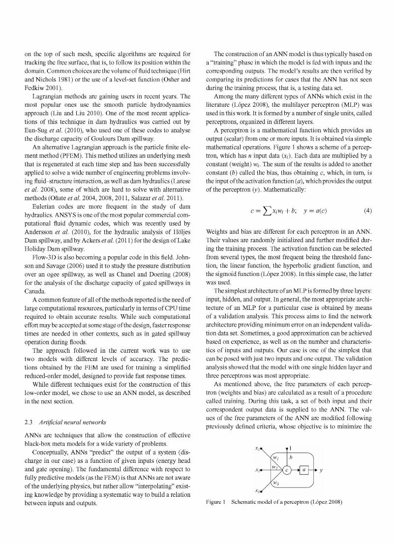
A perceptron is a mathematical function which provides an output ( scalar) from one or more inputs. It is obtained via simple mathematical operations. Figure 1 shows a scheme of a percep-tron, which has n input data (x,-). Each data are multiplied by a constant ( weight) w,-. The sum of the results is added to another constant (b) called the bias, thus obtaining c, which, in turn, is the input of the activation function (a), which provides the output of the perceptron (v). Mathematically:

c = ^x/M'/ + b; v = a(c) (4)

Weights and bias are different for each perceptron in an ANN. Their values are randomly initialized and further modified dur-ing the training process. The activation function can be selected from several types, the most frequent being the threshold func-tion, the linear function, the hyperbolic gradient function, and the sigmoid function (Lopez 2008). In this simple case, the latter was used.

The simplest architecture of an MLP is formed by three layers: input, hidden, and output. In general, the most appropriate archi-tecture of an MLP for a particular case is obtained by means of a validation analysis. This process aims to find the network architecture providing minimum error on an independent valida-tion data set. Sometimes, a good approximation can be achieved based on experience, as well as on the number and characteris-tics of inputs and outputs. Our case is one of the simplest that can be posed with just two inputs and one output. The validation analysis showed that the model with one single hidden layer and three perceptrons was most appropriate.

As mentioned above, the free parameters of each percep-tron ( weights and bias) are calculated as a result of a procedure called training. During this task, a set of both input and their correspondent output data is supplied to the ANN. The val-ues of the free parameters of the ANN are modified following previously defined criteria, whose objective is to minimize the

Figure 1 Schematic model of a perceptron (Lopez 2008)

discrepancy between the already-known outputs and those pre-dicted by the ANN. In our work, the training was carried out using the Quasi-Newton method (Lopez 2008, Lopez etal. 2008) with Broyden-Fletcher-Goldfarb-Shanno training direction and Brent training rate.

3 Methodology

3.1 Numerical FEM model

The examples presented in the current work were run using an Eulerian FEM completed in the open-source code Kratos (Dadvand et al. 2010, Rossi et al. 2011), developed at Centre Internacional de Metodes Numerics en Enginyeria (CIMNE).

The solution module is designed for the resolution of the 3D Navier-Stokes equations using the FEM. In this work, a level-set approach is applied for the simulation of the free-surface problem. The main features of the solver (Rossi et al. 2011) are:

(1) Discretization of the Navier-Stokes equations for incom-pressible fluid using the standard FEM and an Eulerian approach (Zienkiewicz et al. 2005).

(2) Low-order (linear) elements three-noded triangles in two-dimensional (2D) and four-noded tetrahedra in 3D.

(3) Time integration with a semi-explicit version of the fractional-step method (Rossi et al. 2011).

(4) Improvement in mass conservation via an "error recover-ing" technique that allows correcting the solution taking into account the errors made in the previous time steps.

(5) Level-set method (Osher and Fedkiw 2001) for tracking the free surface.

(6) An extrapolation function which allows computing the val-ues of velocity, pressure, and pressure gradient on the nodes in the air region area close to the free surface in the fluid.

The algorithm follows the following steps:

(1) Extrapolate velocity, pressure, and pressure gradient on the analysis domain (including fluid and air subdomains).

(2) Convect the level-set function defining the new free surface on the basis of the velocity field both on fluid and air domains.

(3) Re-initialize the distance function on the whole domain starting from the zero of the level-set function obtained at Step (2).

(4) Solve the momentum equations for the fluid flow. (5) Set the pressure boundary condition so that pressure is

(approximately) zero at the position indicated by zero of the level-set function.

(6) Solve the pressure equation (7) Solve the correction equation (8) Back to Step (1).

Details of the algorithm can be found in Rossi et al. (2011). The code is currently suitable for parallel processing

for shared memory machines (SMMs) using OpenMP. The algorithm is also adequate for distributed memory machines par-allelization, although at the current stage only the SMM version is available.

3.2 ANN

The high computational cost is one of the drawbacks of numerical modelling of 3D hydraulic problems. The key objective of the application of ANN is quasi real-time computation. This would allow the dam owner to compute actual discharges in practical situations (energy head, gate opening).

Currently, the way in which discharge curves are calculated using numerical models is similar to experimental tests: a number of relevant cases are selected and the results are used to obtain general expressions via curve fitting.

In order to optimize the work, a numerical test plan to obtain the discharge curves by extrapolation of the results of 2D models was devised (which computational cost is signifi-cantly lower than 3D runs). A few 3D models were run so as to validate the extrapolation. The steps of this methodology are the following:

(1) 2D numerical modelling of situations corresponding to inte-ger values of the gate opening (£>). For each one of them, four values of the inflow and the correspondent energy head on the crest were computed.

(2) Extrapolation of the results to actual 3D spillway geometry, taking into consideration side contractions. In our work, the expression developed to calculate effective length in free-ogee crests - that is, Eq. (2) - was used.

(3) Numerical modelling of a few representative 3D cases. The goal is to check the accuracy of the extrapolation defined in Step (2).

(4) Creation and training of an ANN based on the numerical results. The ANN allows the user to calculate the outflow for any possible situation (upstream head, gate opening) within the operation range of the spillway.

The ANN was generated and trained using the open-source ANN software OpenNN (Lopez 2012). OpenNN is based on an implementation of the MLP

3.3 Oliana Dam case study

The Oliana Dam spillway was chosen as the test case for the application of the methodology described above. Oliana Dam is located on the Segre River, in Lleida (Spain). Its spillway has two bays, both controlled by 17-m wide by 9-m tall radial gates. The operation range is from crest elevation (509.3 meters above sea level (m.a.s.l.)) to a design head (Hd) of 9.0 m (518.3 m.a.s.l.).

Inflow boundary condition

In the 2D models, inflow discharge is imposed by setting the velocity of the fluid at the boundary of the domain opposite the spillway, so that

qio = vT (5)

where g2D is the unit flow, in m2 s - 1 , v is the velocity at the boundary, in ms - 1 , and T is the length of the boundary line, in m (Fig. 2).

An analogous condition was applied for 3D calculations:

03D = vTB ( 6 )

where Qm is flow, in m3 , v is the velocity in the boundary, in ms - 1 , and T and B are the dimensions of the boundary surface, in m (Fig. 2).

Domain dimensions

One of the parameters which may influence the value of the discharge coefficient is the vertical distance from the spillway crest to the bottom of the domain (P, see Fig. 2 ). According to USBR (1987), the discharge coefficient for free-weir flow is independent of this factor when the ratio P/Hd is greater than 3.

Given that the design head is 9.0 m, and that the P height in Oliana Dam is above 30 m, the actual discharge coefficient in Oliana Dam spillway should not depend on this factor. Thus, the vertical distance from the spillway crest to the bottom of the domain was set to 30 m in all the numerical models, so that they reproduce this effect.

The domain in the downstream side of the gate was restricted to the topmost part of the chute. It was checked to insure that the downstream condition did not affect the discharge coefficient.

A sensitivity study on the influence of the horizontal dimen-sions was carried out for both 2D and 3D models. The objective was to define the limits of the domain, so that the boundary conditions did not affect the results.

A 3-m gate opening was selected for the 2D analysis, with 750 m3 inflow (22.06 m2 unit inflow ). It was run for three different domains having 50, 75 and 100 m measured from the spillway face to the inlet.

Results showed that the difference in terms of energy head between the three models is less than 1 cm, representing around

0.15%. It could therefore be concluded that the smaller domain was large enough to insure that the inlet boundary condition does not affect the results.

A similar analysis was carried out for the 3D models in order to determine the distance W from the abutment to the boundary (Fig. 2 ). Three different 3D domains were used to calculate the free flow case for 500 m3 s - 1 , in which W equalled 10, 20 and 30 m.

Energy head was computed as the average of the water surface elevation (W.S.E) in the area which lies outside the acceleration zone ( where velocity head is negligible). The results showed that the effect of the width increment on the approach head losses was negligible for 20 m ( Table 1). Thus, the intermediate domain was selected for the 3D models.

Energy head measurement and outflow stability All the models started from an initial condition in which the domain was full of water up to the spillway crest. From that moment on, inflow makes the free surface rise, and outflow begins and increases, until the steady-state is achieved ( i.e. inflow equals outflow, and the free surface remains stable). Certain fluctuations were recorded in terms of outflow which were anal-ysed in order to assess their relevance. Outflow discharge was measured by defining a control section under the gate lip, as outlined in Fig. 3.

Figure 4 shows a typical time series plot of discharge, where it can be seen that it becomes stable after around 60 s of simula-tion ( the magnitude of the fluctuations below 1 % of the inflow). Similar behaviour was recorded in 3D cases.

Mesh size Mesh size is one of the key aspects of FEM calculations. The mesh must be fine enough to accurately reproduce the main fea-tures of the flow field. Conversely, the number of elements must be moderate, so that the computational cost is affordable. The latter is equivalent to a lower limit of the mesh size.

Table 1 Energy head for different widths

W (m) 10 20 30

Average W.S.E. (m.a.s.l.) 515.32 515.34 515.34

Figure 3 Detail of the mesh, showing the position of the free surface and the cut under the gate lip

25

20

^ 15 <D 00 &

I 10 -o •a 3

5

0 0 50 100 150 200 250 300 t( s)

Figure 4 Typical discharge time series

When running a fluid dynamics calculation for free-surface flows, it is essential to set a fine mesh in the area where the free surface is expected to be. In this way, its position can be accu-rately computed and possible irregularities can be accounted for. Regions far from the free surface can be meshed using a larger element size.

It is also convenient to set a fine mesh region where significant gradients of the variables (pressure, velocity) are expected to occur. In our work, this happens in the environment of the gate and the crest, as well as in the chute.

The mesh size was defined following the above-mentioned criteria. Thus, 2D models were meshed with 0.25-m-edge triangles for the fine mesh and with 3-m-triangles for the coarse mesh. For 3D models, 0.5-m and 3-m edge tetrahedra were used.

Roughness

The FEM code allows us to model the effect of boundary rough-ness, which is taken into account as the wall law. The value of the wall law parameter was set to match the magnitude of the absolute roughness of the actual boundary, 1 mm.

In our work, given that the velocity does not reach high values ( only the reservoir and the topmost reach of the chute are mod-elled), the wall roughness was expected to have little influence on the results.

3.4 Extrapolation of the results of 2D models

2D numerical models reproduce a unit discharge without side contractions at all. In order to apply 2D results to an actual spill-way, an effective length has to be considered. This should be lower than total length to account for the side contractions that actually occur. Given that there is not a specific expression for calculating the effective length in gated spillways, the empirical formulation which is commonly used for free-flow ogee crests -that is, Eq. (2) - was used in our work. Thus, the discharge is computed as:

Qex = CJ2DL = q2D IL' - 2 (NKp + Ke )He] (7)

where Qex is total discharge (m3 ), q2D is the unit discharge from 2D models (m2s_ 1), L is the effective length calculated using Eq. ( 2 ), in m, and He is the energy head on spillway crest (m). The values of Kp and Ke for Oliana Dam spillway are 0.01 and 0.1, respectively, according to the geometry of the pier and abutments and the criteria of the USBR (1987).

This procedure extrapolates the 2D results, so that they can be applied for obtaining discharge curves for the actual Oliana Dam spillway.

3.5 Calculation of the underflow discharge using ANN

Discharge curves for gated spillways are commonly presented on a chart showing the discharge-head relation for several gate openings. Each curve can be obtained using the results of several computer runs. For the Oliana Dam spillway, four values of the inflow ( covering the whole operation range) and their correspon-dent heads (He) were computed for each integer value of the gate opening (£>), from 1 to 5 m. However, during the reservoir oper-ation, the dam owner needs to know this relation for any value of the energy head and gate opening.

One option to do that is to obtain a mathematical expression yielding the discharge coefficient for any given value of both head and gate opening, via Eq. (3). There is not a general rule for this procedure. It was already shown that the empirical for-mulation does not take into account some of the factors which may influence the discharge curves, such as side contractions or energy head.

An obvious alternative would be to run the numerical simu-lation for the specific situation of interest. This would require the availability of the numerical code and time for the run. Consequently, this approach is not practical.

In order to solve this drawback, ANNs were used to obtain a mathematical expression which computes in a quasi-real time the discharge flow for any given situation (energy head and gate opening) using the results of the numerical tests.

In the Oliana Dam spillway analysis, 20 different situations of gate-controlled discharge were calculated using the FEM, com-prising 1, 2, 3, 4 and 5 m gate openings. Given that these data seemed to be too scarce to be used as training data, a greater input data set was generated. It was found that an interpolating

polynomial could be obtained via curve fitting for computing the head-discharge relation for each gate opening ( with a root-mean-square error below 1%). These expressions were used to generate the input data set. One hundred data sets were generated in this way (20 for each integer value of the gate opening), covering the entire operating range of the spillway ( from 0 to 9.0 m of energy head). Of which, 60% of them were used for training, and the rest for testing.

The ANN training process was performed using supervized learning (Lopez 2008). In this kind of training algorithm, both the inputs and the corresponding outputs of the training data set are supplied to the ANN. The initial values of the free parameters are randomly defined. Then, the ANN takes the input values (energy head and gate opening), modifies the free parameters, obtains a result, and compares it with the correct ones ( discharge) which were supplied. This process is repeated until the root-mean-square error in the training data set becomes lower than 10~6. Finally, the model's results are verified by comparing its predictions for the testing data set.

Once the training process is successfully completed, the ANN can be used to calculate, in a very fast manner, the discharge for any given gate opening within the range of the training data ( i.e. between 1 and 5 m). If a gate opening lower than 1 m or greater than 5 m is used, the ANN provides an output (extrapolation) which in general will be wrong. As a general rule, the ANN should not be applied outside the range of the training data set.

4 Results and discussion

4.1 Empirical formulation

Discharge curves for Oliana Dam spillway were computed using the empirical formulation suggested by USACE (1992), as described above.

4.2 Numerical modelling

2D FEM analyses were carried out for 20 different situations having gate openings from 1 to 5 m, and covering the whole range of energy head of the spillway for an underflow discharge (Fig. 5). The 2D models do not consider side contractions. The curves joining the output points have the typical shape: they are quasi-vertical for 1 -m gate opening, and tend to a horizontal line for larger openings.

These results were extrapolated to Oliana Dam spillway mul-tiplying the computed unit discharge by the effective length calculated using Eq. (2). The outcome is a family of curves of similar shape, which were compared with the results of the 3D models. Figure 6 shows this comparison.

The 3D FEM results for underflow discharge match the pre-dictions of the extrapolations of 2D results within about 1%. This strongly suggests that the expression for calculating the effective length developed for free-flow ogee crests is a good

520

S. 518 a o | 516 U w H 514

3 00

S3 512

510 0 10 20 30 40 50

Discharge (m2s_1)

Figure 5 Results of 2D models. Unit discharge

520

I 518

a 0 1 516 > <D m <D

514 <4-1 u oo

512 a •S

510

0 500 1000 1500 2000 Discharge (m3 s_1)

Figure 6 Comparison between extrapolation of 2D results and 3D results

approximation to account for the side contractions in underflow discharges.

4.3 ANN analysis

The ANN predicts the underflow discharge for any value of the energy head and gate opening within the range of the training data. Figure 7 shows the outputs of the ANN analysis for 1, 1.5, 2, 2.5, 3, 3.5, 4, 4.5 and 5 m gate openings in comparison with the numerical results (extrapolations of 2D results). The ANN predictions match the numerical results with an accuracy of 1%. In addition, the results for intermediate gate openings are reasonable.

4.4 Empirical vs. numerical results

In general, the discharge predicted by the empirical formula is lower than the result of the numerical models for a given gate opening and energy head. Figure 8 shows the comparison between both predictions, and Table 2 includes the difference both in percentage and in absolute value. The table shows the mean value of the cases analysed for each gate opening.

D= lm—e-D = 2m—*-D = 4m x D = 5m - b £> = 3m —

10

- 8 S. U 6 00 ^ < % 4 w

2

0 0 200 400 600 800 1000 1200 1400 1600

Discharge (ill's-1) Figure 7 ANN vs. numerical results

520

£ 518 C

| 516

| 514 cw

1 512 S

510

0 500 1000 1500 2000 2500 Discharge (m3s - 1)

Figure 8 Discharge curves for Oliana Dam spillway: (a) using empir-ical formulation; (b) extrapolating 2D numerical models; (c) from 3D numerical models. The curve for free discharge was obtained using Eqs. (1) and (2)

Table 2 Average difference between empirical and numerical predictions of gated-discharge flow for Oliana Dam spillway

Gate opening (m) 1 2 3 4 5

\(Qg ~ Qex)\("l3 S-1) 16 22 31 39 12

1 (Qg- Qex)\/Qex(%) 6.7 4.3 3.9 3.8 0.7

5 Summary and conclusions

Discharge curves for Oliana Dam spillway were calculated using numerical simulation. An Eulerian FE code developed at CIMNE was used. The relation between head and unit discharge for 1, 2, 3,4 and 5 m gate openings was obtained from the results of 2D FE models. These results were extrapolated to the actual geometry of Oliana Dam spillway multiplying the unit discharge by an effective length. The latter was computed using the empirical formulation developed for free-flow ogee crests, that is, Eq. (2 ).

Four different situations of inflow-gate opening were com-puted using a 3D FE model for assessing the accuracy of the 2D extrapolation. The results are within 1 % of those extrapolated from the 2D FE model.

The same curves were computed using the empirical formula-tion developed by USACE (1992) and recommended by USBR (1987) and SPANCOLD (1997). FEM results differ less than 7% in terms of discharge ( Table 2).

An ANN was developed and trained on the basis of the results of numerical models. The ANN reproduces FEM results with an accuracy of 1%, and yields reasonable approximations to the discharge curves for intermediate openings.

The key conclusions of this work are summarized below.

(1) The formulation for computing the effective length in free-flow spillways can be a good approximation for calculating underflow discharge curves based on the results of 2D FE models. However, further research is needed to check if it provides accurate results for alternate combinations of number of bays, geometry of piers and abutments, energy head, etc.

(2) The FEM can be useful in the calculation of the discharge capacity of spillways. In order to increase confidence in the results, information on either experimental or on site data for the Oliana Dam spillway would be needed.

(3 ) ANNs can be a useful tool for the quasi real-time calculation of the response of a spillway system on the basis of discrete data given by numerical (or experimental) tests.

Acknowledgements

This research was partially supported by the SAFECON project of the European Research Council (ERC), as well as by the ALCON project (ref. IPT-310000-2010-11) funded by the Span-ish Ministry of Economy and Competitiveness (MINECO) and the European Regional Development Fund (ERDF). Special thanks are due to Gonzalo Rabasa (Confederation Hidrografica del Ebro) and Francisco Riquelme (INHISA) for promoting this research.

Notation

a = activation function of a perceptron (—) B = horizontal dimension of the inflow boundary

condition (m) b = bias of a perceptron (—) c = input of the activation function in a perceptron (—) C = discharge coefficient for free flow (m1/2 ) Q = discharge coefficient for gated flow (—) D = gate opening (m) g = gravitational acceleration (ms~2) H = energy head to the centre of the orifice ( m) Hd = design head (m) He = energy head on the crest ( m) Kp = pier contraction coefficient (—) Ke = abutment contraction coefficient (—) L = effective length of the spillway ( m) L< = total length of the spillway ( m) N = number of piers (—)

D(m) 1.0 1.5 2.0 2.5 3.0 3.5 4.0 4.5 5.0

ANN o FEM —

n = number of inputs of an ANN (-) P = vertical distance from the crest to the bottom of the

domain (m) Ql = free-flow discharge (m3 s - 1 ) g 3 D = discharge in 3D models (m3 ) Qg = empirical gate-controlled discharge (m3 s_ 1) Qex = discharge extrapolated from 2D models (m3 )

= discharge in 2D models (m2 ) S = total area of the orifice in underflow

discharge (m2) T = vertical dimension of the inflow boundary

condition (m) 9 = angle formed by the tangent to the gate lip and the

tangent to the crest curve (°) v = inflow velocity (ms -1) W = distance from the abutment to the boundary in 3D

models (m) Wj = weights of inputs jc, to a perceptron (-) %i = inputs to a perceptron (-) y = output of a perceptron (-)

References

Ackers, J., Bennet, F., Zamesky, G. (2011). Upgrading Lake Holiday spillway using a labyrinth weir [online], Proc. 31st Annual USSD Conference, San Diego, California, 1683—1696, M.F. Rogers, ed. Denver. Available from: http://ussdams.com/proceedings/201 lProc/1683-1696.pdf (Accessed 15 November 2012).

Andersson, A.G., Lundstrom, K., Andreasson, P., Lundstrom, T.S. (2010). Simulation of free surface flow in a spillway with the rigid lid and volume of fluid methods and validation in a scale model. Proc. VEuropean Conference on Computational Dynamics, Lisbon, 14—17, J.C.F. Pereira and A. Sequeira, eds. Lisbon, Portugal.

Chanel, P.G., Doering, J.C. (2008). Assessment of spillway mod-eling using computational fluid dynamics. Can. J. Civ. Eng. 35(12), 1481-1485.

Dadvand, P., Rossi, R., Onate, E. (2010). An object-oriented environment for developing finite element codes for multi-disciplinary applications. Archiv. Comp. Met. Eng. 17(3), 253-297.

Eun-Sug, L., Violeau, D., Issa, R., Ploix, S. (2010). Application of weakly incompressible and truly incompressible SPHto 3-D water collapse in waterworks. J. Hydraulic Res. 48(Suppl. 1), 50-60.

Frizell, K.W., Kubitschek, J.P, Einhellig, RF. (2009). Folsom dam joint federal project. Existing spillway modeling. Dis-charge capacity studies. HL-2009-02 [online], U.S. Bureau of Reclamation.

Hirt, C.W., Nichols, B.D. (1981). Volume of fluid (VOF) method for the dynamics of free boundaries. J. Comput. Phys. 39(1), 201-225.

Johnson, M.C., Savage, B.M. (2006). Physical and numerical comparison of flow over ogee spillway in the presence of tailwater. J. Hydraulic Eng. 132(12), 1353-1357.

Larese, A., Rossi, R , Onate, E., Idelsohn, S.R (2008). Validation of the particle finite element method (PFEM) for simulation of free surface flows. Engineering Computations, 25 385-425.

Liu, M.B., Liu, G.R. (2010). Smoothed particle hydrodynamics (SPH): An overview and recent developments. Archiv. Comp. Met. Eng. 17(1), 25-76.

Lopez, R. (2008). Neural networks for variational problems in engineering. PhD Thesis, Department of Computer Languages and Systems, Technical University of Catalonia, Spain.

Lopez, R. (2012). OpenNN: Open Neural Networks Library (Version 0.9) [software]. Retrieved from http://flood. sourceforge.net.

Lopez, R., Balsa-Canto, E., Onate, E. (2008). Neural networks for variational problems in engineering. Int. J. Num. Met. Eng. 75(11), 1341-1360.

Onate, E., Idelsohn, S.R., Del Pin, F., Aubry, R. (2004). The particle finite element method: An overview. Int. J. Comput. Met. 1(2), 267-307.

Onate, E., Idelsohn, S.R, Celigueta, M.A., Rossi, R. (2008). Advances in the particle finite element method for the anal-ysis of fiuid-multibody interaction and bed erosion in free surface flows. Comp. Meth. Appl. Mech. Eng. 197(19-20), 1777-1800.

Onate, E., Celigueta, M.A., Idelsohn, S.R., Salazar, F., Suarez, B. (2011). Possibilities of the particle finite element method for fluid-soil-structure interaction problems. Comput. Mech. 48(3), 307-318.

Osher, S., Fedkiw, R. (2001). Level set methods: An overview and some recent results. J. Comput. Phys. 169(2), 463-502.

Rossi, R., Larese, A., Dadvand, P., Onate, E. (2011). An effi-cient edge-based level set finite element method for free surface flow problems. Int. J. Num. Meth. Fluids, [online], http://dx.doi.org/10.1002/fld.3680

Salazar, F., Onate, E., Moran, R. (2011). Modelacion numerica de deslizamientos de ladera en embalses mediante el Metodo de Particulas y Elementos Finitos (PFEM). Rev. Int. Met. Num. Ing. 28(2), 112-123.

SPANCOLD. Spanish Committee on Large Dams. (1997). Guia Tecnica de Seguridadde Presas n° 5. Aliviaderosy Desagues, CNEGP, Madrid, Spain.

US Army Corps of Engineers (1992). Hydraulic design of spillways. EM 1110-2-1603, Department of the Army, Wash-ington, DC.

United States Bureau of Reclamation (1987). Design of small dams. ed. 3. U.S. Government Printing Office, Washing-ton, DC.

Zienkiewicz, O.C., Taylor, R.L., Nithiarasu, P. (2005). The finite element method for fluid dynamics, ed. 6. Elsevier Butterworth-Heinemann, Oxford, UK.