ANALYSIS OF THE CHANGES IN CHEMICAL …2015)/p.317-332.pdf · ANALYSIS OF THE CHANGES IN CHEMICAL...

CELLULOSE CHEMISTRY AND TECHNOLOGY

Cellulose Chem. Technol., 49 (3-4), 317-332(2015)

ANALYSIS OF THE CHANGES IN CHEMICAL PROPERTIES OF

DISSOLVING PULP DURING THE BLEACHING PROCESS USING

PIECEWISE LINEAR REGRESSION MODELS

OLIVER BODHLYERA*, TEMESGEN ZEWOTIR*, SHAUN RAMROOP* and

VIREN CHUNILALL**

*School of Mathematics, Statistics and Computer Science,

University of KwaZulu-Natal, P Bag X01, Scottsville 3209, Pietermaritzburg, South Africa **

The Forestry and Forest Products Research Centre, CSIR-Durban, South Africa

Corresponding author: Oliver Bodhlyera, [email protected]

Received February 17, 2014

Dissolving wood pulp is a chemically bleached wood pulp that has a cellulose content of more than 90%. Such pulp has

certain properties of industrial value according to the products it can be used for. Raw pulp, which comes after acid

bisulphite pulping, goes through a number of bleaching processing stages, each with a specific role, to produce

dissolving pulp. These processing stages have different effects on the pulp depending on the type of wood genotype

that is being processed. The bleaching processing stages are considered as time points for repeated measurements of the

following chemical properties viz., viscosity, lignin, γ-cellulose, α-cellulose, copper number, glucose and xylose.

Piecewise regression models were used to compare the behaviour of the chemical properties of the seven genotypes

throughout the bleaching processing stages. In order to cut costs on the chemicals used for processing, it is important to

identify species/genotypes that have similar chemical properties under the chemical pulping process in order to mix

them together for optimised processing. It was established that when trying to classify different timber

species/genotypes for the purpose of finding which ones can be mixed together, viscosity is not an important variable to

consider. The other variables viz., lignin, γ-cellulose, α-cellulose, copper number, glucose and xylose should be used

for classification as they were found to be important for that purpose. It is suggested that these properties can also be

used in multivariate classification procedures.

Keywords: dissolving pulp, piecewise linear regression, lignin, viscosity, γ-cellulose, α-cellulose, copper numbers,

glucose and xylose

INTRODUCTION Dissolving wood pulp is a bleached pulp with

more than 90% pure cellulose fibre.1 Cellulose is

the fibre component in wood that is obtained

through pulping and bleaching processes. This

pulp has a high level of brightness and uniform

molecular weight distribution and it is used to

make products such as viscose, rayon, acetate

textile fibres, cellophane and many other chemical

products.2 Delignification through pulping and

bleaching removes lignin, hemicellulose and other

impurities and results in high purity α-cellulose

pulp fibre, which can be used in the manufacture

of the above mentioned products. Sharma and

Shukla3 state that the delignification process aids

in the removal of the structural polymer lignin

from wood pulp, resulting in higher purity

cellulose. Bleaching follows after the

delignification process to further remove residual

lignin from the pulp. During the process of

extracting lignin through delignification and

bleaching, other chemical properties are also

altered, namely pulp viscosity, glucose level,

degraded celluloses, hemicelluloses, and other

chemical properties of which some are discussed

in this study.

The process of chemical pulping to produce

dissolving pulp has a very low solid matter yield

(30% to 35%).4 Chemical pulping takes place in a

high temperature and pressure environment with

chemicals added to dissolve lignin and

hemicelluloses, which are then washed away.5

The partial dissolution of lignin, which glues the

wood fibres together, results in the cellulose

OLIVER BODHLYERA et al.

318

fibres separating from each other. Lignin removal

is important because its presence imparts a

yellowish brown colour to the pulp. This is an

undesirable property of the dissolving pulp since a

high level of brightness is important in the

production of cellulose based products, such as

viscose and acetate fibres.

Since the chemicals used in pulp processing

are costly, it is necessary to optimise the usage of

such chemicals by identifying and combining

wood species/genotypes with similar chemical

properties under the chemical pulping process.

This study tries to identify such species/genotypes

by modeling the chemical properties of dissolving

pulp at all the processing stages using piecewise

linear regression models. Piecewise linear

regression models are deemed appropriate for

these data, since there are three known sub-

processes, in series, in the chemical processing of

dissolving pulp, namely, delignification,

bleaching and finishing. Species/genotypes with

similar rates of change (or slopes) in the chemical

property under consideration during the three sub-

processes will be mixed together during

processing in the future if economic quantities

cannot be achieved with just one

species/genotype. Species/genotypes that differ

significantly in the way they respond to the

processing stages would better be processed

separately. It is expected that each of the three

sub-processes will have a different effect on the

response variables, hence the resultant models are

three segment, piecewise linear regression

models. In this study, the response variables are

seven important chemical properties of dissolving

pulp and the independent variable is the stage of

processing.

The main objective in the processing of

dissolving pulp is to remove lignin, retaining α-

cellulose, while at the same time maintaining

other properties like viscosity within certain

product specified limits. The modeling, for each

species/genotype, of how lignin, viscosity, γ-

cellulose, copper number, and xylose content

decrease over the processing stages and of how α-

cellulose and glucose increase will highlight the

differences in species/genotype responses to

chemical processing of dissolving pulp.

Pulping process

In order to understand the nature of the data, it

is necessary to understand the chemical pulping

process in detail. In a pulping process, wood is

converted into fibres. This can be achieved

mechanically, thermally, chemically or through a

combination of these techniques.6 Chemical

delignification, an important process during

pulping, includes all processes resulting in partial

or total removal of lignin from wood by the action

of suitable chemicals.7 The lignin macromolecule

is depolymerised through the cleavage of the ether

linkages to become dissolved in the pulping

liquor. The α-hydroxyl and α-ether groups are

readily cleaved under simultaneous formation of

benzilium ions.8 The cleavage of the open α-aryl

ether linkages represents the fragmentation of

lignin during acid sulphite pulping. The benzilium

ions are sulphonated by the attack of hydrated

sulphur dioxide or bisulphite ions, resulting in the

increased hydrophylic nature of the lignin

molecule. The extent of delignification depends

on the degree of sulphonation as well as the

depolymerisation8. In summary, the aim of

pulping is to break down the lignin bonds

between the fibres using chemicals and heat,

enabling easy removal by washing, whilst not

destroying the cellulose and hemicellulose

components. The removed lignin is a by-product

that can be used in water treatment, dye

manufacture, agricultural chemicals and in road

construction.9 Different wood species/genotypes

have different levels of lignin content and those

species/genotypes that contain more lignin would

require more reagents to extract the lignin from

the cellulose.10

This means that different wood

species/genotypes have different lignin extraction

behaviour as they go through the chemical

processing stages and it is of interest to

investigate this behaviour. The wood

species/genotypes with similar physical and

chemical characteristics would naturally be put

into the same class and may be mixed during

processing if larger processing quantities are

needed.

Bleaching process The laboratory bleaching sequence was a

scaled down version of the commercial process.

The results obtained for the viscosity and lignin

content (K-number) at the oxygen delignification

(O) stage were used to adjust the bleaching

conditions. The chemical pulping and bleaching

process considered here consists of six stages, as

indicated in Table 1 below. For the purposes of

this study, the first stage will be called the O-

stage, i.e., the stage where wood is acid bisulphite

pulped into raw material for the bleaching stages.

Pulp

319

Table 1

Stage classification for statistical analysis purposes

Stage Process Description

0 Wood to raw pulp Delignification

1 O Delignification

2 D1 Brightness

3 E0 Extraction of hemicelluloses and solubilisation

of lignin degradation products

4 D2 Brightness

5 P Brightness and residual hemicellulose removal

Figure 1: Processing stages and the pulp samples

The aim of adjusting the bleaching conditions

was to produce dissolving pulp that would meet

the quality control parameters for α-cellulose,

viscosity, copper number, glucose (%) and xylose

(%) prescribed commercially for the 96α

dissolving pulp grade. While it would be

reasonable to consider the correlated chemical

properties using multivariate techniques, this

study looked at a single chemical property

individually with the aim of modelling and

comparing the behaviour of wood

species/genotypes on the same chemical property.

Data The wood species/genotypes analysed in this

study are E.dunnii, E.grandis, E.nitens, E.smithii

and the Eucalyptus clones E.gc, E.guA and

E.guW. The variable species/genotype is a fixed

effect with seven levels, namely the seven

genotypes that are known beforehand. The

subjects are the pulp samples taken from pulped

wood species/genotypes.

Trees were randomly selected from each of the

seven species/genotypes, chipped and raw pulp

was produced through acid bisulphite pulping.

Independent samples were then taken from the

raw pulp and processed. From each sample,

measurements of various chemical properties

were recorded at the six processing stages

described in Table 1, and are shown in Figure 1.

The samples were processed using three different

bleaching conditions coded as A, B and C.

Bleaching condition A is a set of original

bleaching conditions, whereas bleaching

conditions B and C are revised sets of bleaching

conditions specially set to ‘fine tune’ non-

conforming final pulps. If the chemical properties

of the final product do not fall within prescribed

limits, then the product will not be put on the

market. This, in a way, produced a controlled

response variable, especially at the final stage of

production. The bleaching conditions were found

not to be significantly different, hence they are

not a prominent part of this study. The pulp

samples are random effects, as trees were chosen

at random from a large number of possible trees.

EXPERIMENTAL The six stages in the chemical process fall under

three sub-processes, namely, delignification, bleaching

and finishing and these were carried out under

laboratory conditions as described below.

Delignification: acid bisulphite pulping The cooking liquor was prepared from acid

bisulphite by bubbling SO2 MgO slurry and circulated

in the digester with wood chips. The temperature was

ramped to 140 °C and maintained for a period of time.

The pressure in the digester was kept at 8.5 bars during

the cooking process. At the end of the cooking period,

the reaction mixture was allowed to cool down to room


320

temperature. After pulping, an oxygen delignification

step was included in a rotating digester. Pulp charge

was 800 g (oven dry); consistency 11%; temperature

100 °C; time at 100 °C = 80 min (96α pulp).

Laboratory bleaching and finishing

The oxygen delignified pulp samples were

bleached to target 96α grade using the following

bleaching process: D1 stage (ClO2 treatment), E stage

(NaOH treatment), D2 stage (ClO2 treatment), and a

peroxide stage.

Wet Chemistry analysis – chemical properties In the current study, the quality control parameters

were measured during each step of processing, as

described below.

Cellulose content

Low molecular weight carbohydrates

(hemicellulose and degraded cellulose) can be

extracted from pulp samples using sodium hydroxide.

The solubility of a pulp in alkali thus provides

information on the degradation of cellulose and loss or

retention of hemicellulose during the pulping and

bleaching processes. Thus, it gives an indication of the

amount of degraded cellulose/short chain glucan and

hemicellulose present in the pulp. S10 (%) and S18 (%)

indicate the proportions of low molecular weight

carbohydrates that are soluble in 10% and 18% sodium

hydroxide, respectively. The former alkali solubility

gives an indication of the total extractable material,

that is, degraded cellulose/short chain glucan and

hemicellulose content in a pulp sample, while the latter

alkali solubility gives an indication of the total

hemicellulose content of the pulp sample and is also

known as the percentage gamma (γ%) cellulose

content of pulp samples.

The quantity of degraded cellulose/short chain

glucan, also known as percentage beta (β%) cellulose,

was determined by the difference between S10 (%) and

S18 (%) alkali solubilities, that is,

Degraded cellulose/short chain glucan = S10 (%) – S18

(%).

The α-cellulose content is given by the following

equation:

α-cellulose =

+−

2

%%100

1810 SS

(1)

S10 (%) and S18 (%) alkali solubilities were

determined according to TAPPI method T235 OM-

60.11

The principle of the method is based on the

extraction of carbohydrates with sodium hydroxide

followed by oxidation with potassium dichromate. The

procedure for S10 (%) alkali solubilities determination

is as follows: 1.6 g of the pulp sample is placed in 100

mL of 10% sodium hydroxide (18% sodium hydroxide

for S18 (%) determination). The pulp and solution are

stirred for a period of 3 minutes and thereafter left at

20 ºC for a period of an hour. The pulp sample is

filtered under vacuum using a sintered glass crucible

(G3). Ten millilitres of 0.4N potassium dichromate and

30 mL of concentrated sulphuric acid are added to 10

mL of the filtrate. Thereafter 500 mL of deionised

water is added and the solution is cooled.

Approximately 20 mL of 10% potassium iodide is

added to the cool solution and 5 minutes thereafter the

solution is titrated with 0.1N sodium thiosulphate. A

blank, without pulp sample, is also titrated to give a

blank titre. The alkali solubility is given by the

following equation:

Alkali solubility = samplepulpofWeight

titreSampletitreBlank %685.0)( ×−

(2)

Viscosity The viscosity of a pulp sample provides an estimate

of the degree of polymerisation (DP) of the cellulose

chain. Viscosity determination of pulp is one of the

most informative procedures, which are carried out to

characterise a polymer, i.e., this test gives an indication

of the degree of degradation (decrease in molecular

weight of the polymer, i.e. cellulose) resulting from the

pulping and bleaching processes. The viscosity

measure involves dispersing 1 g of dissolving pulp

sample (cellulose I) in a mixture of (15 mL) sodium

hydroxide and (80 mL) cuprammonium solution

(concentration of ammonia 166 g/L and concentration

of copper sulphate 94 g/L) for a period of 1 hour. The

dispersed cellulose I is allowed to equilibrate at 20 ºC

for 1 hour and is then siphoned into an Ostwald

viscometer. The time taken for it to flow between two

measured points is recorded and the viscosity is

calculated using the specific viscometer coefficient at

the corresponding temperature according to a TAPPI

method.12

Lignin content (k-number) The permanganate number (k-number method) was

used to assess the lignin content after each stage of

processing. The principle of the method is based on the

direct oxidation of lignin in pulp by standard

potassium permanganate and back-titrating the excess

permanganate with ferrous ammonium sulphate

(Mohr’s salt) standard solution.13 The procedure for

permanganate number determination is as follows:

approximately 20 mL of 10% sulphuric acid and 180

mL of water are added to 1 g of pulp sample in a

conical flask. The mixture is then stirred using a

magnetic stirrer. Twenty five millilitres of 0.1N

potassium permanganate is added and after 3 minutes

25 mL of 0.1N ferrous ammonium sulphate is added,

followed by 10 drops of N-phenyl anthranilic acid

indicator. The excess is back titrated with 0.1N

potassium permanganate. A blank is also carried out

with the exception of the pulp sample. The following

calculation is used for permanganate number

determination:

Permanganate number = (Sample titre – Blank titre) x

0.355

Pulp

321

The data were modelled using piecewise linear

regression models that represented the three sub-

processes, namely delignification, bleaching and

finishing.

Copper number (Cu number)

Pulping and bleaching are known to affect cellulose

structure by the generation of oxidised positions and

subsequent chain cleavage in pulp samples.14

The

copper number gives an indication of the reducing end

groups in a pulp sample. The copper number is a

measure of the reducing properties of the pulp and is

defined as the number of grams of metallic copper

reduced from the cupric (Cu++) to cuprous (Cu+) state

in alkaline solution by 100 g cellulose under standard

conditions. The copper number is inversely

proportional to the viscosity of the pulp samples, that

is, with a decrease in viscosity there is increased chain

cleavage and hence more reducing end groups. The

copper number also serves as an index of reducing

impurities in pulp, such as oxycellulose,

hydrocellulose, lignin and monosaccharides, which

possess reducing power. The procedure for

determining copper number is as follows: 2.5 g of

disintegrated pulp is mixed with a

carbonate/bicarbonate (2.6/1, w/w) and 0.4N copper

sulphate solution (95/5, v/v) for exactly 3 hours.

Thereafter the pulp is filtered and washed with 5%

sodium carbonate followed by hot deionised water.

Cuprous acid is dissolved by treating the cellulose on

the filter with 45 mL of 0.2N ferric ammonium

sulphate. This is left for 10 minutes then filtered off.

The pulp is then washed with 250 mL of 2N sulphuric

acid. The filtrate is then titrated with 0.04N KMnO4.

The blank is subtracted from the titre value to yield the

number of grams of reduced copper in the pulp

sample.15

Glucose and xylose The polysaccharides were measured after their

conversion to monosaccharides (glucose and xylose)

via a two-step hydrolysis procedure with 72%

sulphuric acid. The first step in the hydrolysis process

is the addition of 3 mL of sulphuric acid to 0.2 g of

oven dried pulp in a test tube with stirring. The

contents of the test tube are then quantitatively

transferred into a Schott bottle with 84 mL of water.

The second step in the hydrolysis process involves

placing the Schott bottle in an autoclave set at a

temperature of 121 ºC and pressure of 103 kPa for 1

hour. The contents are then allowed to cool and then

filtered using a 0.45 µm filter. The filtrate is then

transferred to a 200 mL volumetric flask and diluted to

the mark. 50 µl of the sample is placed in a vial and

diluted with 500 µl of water. Twenty microlitres of 1

mg/ml fucose (internal standard) is added using the

autosampler. The monosaccharide constituents

(glucose, mannose, xylose, arabinose etc.) were

analysed using high performance liquid

chromatography coupled with pulsed amperometric

detection.16 Reference standards of glucose and xylose

were prepared. The standards were treated in the same

way as the sample and analysed using high

performance liquid chromatography coupled with

pulsed amperometric detection. The concentrations of

the monosaccharide constituents were obtained from

the calibration curves of the standards.

RESULTS AND DISCUSSION

Graphical presentation of chemical properties

over processing stages Figure 2 shows the percentage content of α-

cellulose as the processing stages unfold. It is

apparently clear from Figure 2 that the change in

α-cellulose percentages increase from the first to

the last stage for all species/genotypes. Generally,

stage D1 has the effect of slightly reducing the α-

cellulose level for all species/genotypes.

The relationship between α-cellulose content

and processing stage is not easy to generalize for

all species/genotypes, hence the statistical method

discussed in this study seeks to describe the

patterns in the data. Different species/genotypes

are expected to have varying model parameters

for the piecewise linear regression model.

Species/genotypes with parameters that do not

differ significantly can be classified as having

similar response profiles to the processing stages

of the chemical pulping process and such

species/genotypes will require similar amounts of

chemicals in each of the six processing stages.

Figure 3 shows how γ-cellulose levels for

different species/genotypes evolve over the

processing stages. The graph for γ-cellulose

(Figure 3) is more of an inverted version of the

graph of α-cellulose (Figure 2). This is due to the

fact that α-cellulose is closely associated with γ-

cellulose and degraded cellulose.

The viscosity profiles for the various

species/genotypes as shown in Figure 4 indicate a

general declining trend over the processing stages.

The process is designed to reduce the viscosity of

the product until ideal characteristics are

achieved. A final product with pulp characteristics

outside the product specific margins is discarded.

For the 96α pulp, the pulp characteristics should

be within the limits outlined in Table 2.

Lignin content for all species/genotypes under

study decreases over the processing stages, as

shown in Figure 5.

The decrease in lignin is not linear over the six

stages, but can be piecewise linear if the stages


322

are grouped into sub-processes, namely

delignification, bleaching and finishing.

Figure 6 shows that copper numbers decrease

with each processing stage with the O2 and E0

stages, accounting, to a greater extent, for the

decrease in copper numbers. It is also clear from

this graph that the species/genotypes do not vary

much in their copper numbers as the lines are very

close together.

Figure 2: Mean α-cellulose content (in %) by stage for

different genotypes Figure 3: Mean γ-cellulose content (in %) by stage for

different genotypes

Figure 4: Mean viscosities (centipoise (cP)) by stage

for different genotypes Figure 5: Mean lignin content (k-number) by stage for

different genotypes

Table 2

Ideal pulp characteristics for 96α pulp

Final pulp

characteristic

Ideal levels

Viscosity (cP) 28 - 35

Copper Number 0.43 - 0.54

S10 6.4 - 7.0

S18 2.7 - 3.3

S10-S18 3.7

α-cellulose >95.3

K-number 0.25

Mean glucose levels, as indicated in Figure 7,

increase as the processing stages unfold with

E.grandis and GuW having higher glucose levels

across the stages than the other five

species/genotypes.

Figure 8 shows the changes in xylose over the

processing stages. It was observed that mean

xylose levels decrease as the processing stages

unfold with E.grandis and GuW having closer and

lower means by stage.

Pulp

323

These two species/genotypes also had very

similar α-cellulose, γ-cellulose, lignin and copper

numbers levels. Based on this similarity, the two

genotypes can be deemed mixable during

processing.

Figure 6: Mean copper numbers by stage for different genotypes

Figure 7: Mean glucose by stage for different

genotypes

Figure 8: Mean xylose by stage for different genotypes

Piecewise linear regression

The data representations in Figures 2 to 8

show that there is a degree of non-linearity in the

data. The piecewise linear regression approach is

a useful method to model such data using two or

more piecewise linear splines.17

It is more

appropriate to use this method for the pulp

processing data, since there are three basic sub-

processes in the whole chemical pulping process

and there will be a spline for each of these sub-

processes in the model. The transition points or

knots are points where the parameters of the

model change from one spline to the other giving

the model a broken stick appearance.18

The three

sub-processes are:

(i) delignification,

(ii) bleaching and

(iii) finishing (peroxide stage)

The delignification sub-process is activated at

the O stage followed by the bleaching sub-process

spanning stages D1, Eo and D2, and the finishing

sub-process, which is activated at the last stage

(where peroxide is used). The variable t1 is used

to represent the delignification sub-process, t2 for

the bleaching and t3 for the finishing sub-

processes. The values of t1, t2 and t3 for each sub-

process are as defined in Table 3. The whole

process can be described in terms of t1, t2 and t3

by equation (3) below:

++++

+++

++

=

final )3(

bleaching )(

ationdelignific

33210

2210

110

et

et

et

Y

ββββ

βββ

ββ (3)

where the values of t1, t2 and t3 are as shown in

Table 3. The response variable Y is the pulp

characteristic of interest, seven of which are

modelled independently in this study, viz.,

viscosity, lignin, γ-cellulose, α-cellulose, copper


324

numbers, glucose and xylose. It is assumed that

the error terms (e’s) within each pulp sample are

correlated at different processing stages according

to a suitable covariance structure, which will be

determined by choosing one with the lowest AIC

value.19

Chemical pulp processing is a continuous

process, and measurements on the seven chemical

properties under study were taken at six time

points or stages (see Table 1). The knots of the

piecewise regression model are set as the stages at

which a different sub-process starts. This is so

because each sub-process has a different effect on

the chemical properties. There are two knots that

separate the three sub-process and these are stages

2 and 5, as indicated in Table 1. Instead of fitting

the piecewise linear regression model with one

covariate (stage as indicated in Table 1) together

with two indicator variables for the two knots,

time or stage is recoded into three time variates.

Each of the new time variates is set to zero when

the sub-process it represents begins.

In equation (3) above, β1, β2 and β3 are rates of

change of the response variable due to

delignification, bleaching and the finishing stage,

respectively. Since delignification occurs at the

raw pulp and the O stages, to be followed by

bleaching thereafter, we let t1=0 for the raw stage

and t1=1 from the O stage up to the finishing stage

as the delignification sub-process ends at the O

stage. The bleaching sub-process begins at stage

D1 (t2=1) and continues in stages E0 (t2=2) and D2

(t2=3). In the finishing stage, there is no bleaching

occurring so t2 remains unchanged at t2=3. A

value of ti=0 for i=1, 2 or 3, indicates that

chemical sub-process ti has not been activated and

if ti remains constant for subsequent stages then

the chemical sub-process ascribed to ti has

stopped. For example t1 remains at t1=1 for stages

O, D1, Eo, D2 and the finishing stage because it is

activated only at stage O and does not occur in

subsequent stages.

The intercept of the delignification sub-

process is β0 with slope parameter β1 and the

intercept of the bleaching sub-process is (β0+β1),

since these are the predicted values of the

response variable when delignification and

bleaching start, respectively. In the same way the

intercept of the finishing sub-process

is 210 3βββ ++ . Equation (3) together with the

values of t1, t2 and t3, as outlined in Table 3, can

be generalised as:

3322110)( tttYE ββββ +++=

(4)

where β0 (the delignification intercept) is the

initial value of the response variable in the raw

stage. The parameters β1, β2 and β3 can be

compared for different species/genotypes to see

which species/genotypes have the same response

rates to the three sub-processes in the chemical

pulp processing.

Analysis of the chemical pulp properties data

for the 96α pulp The SAS procedure Proc Mixed

20 was used to

analyse the data and the results are presented in

the sections that follow. The procedure Proc

Mixed in SAS has the versatility to be used for

the computation of parameter estimates for

various models that include repeated measures

models, such as random coefficient models and

piecewise regression models.21

Piecewise regression models were fitted to the

data for viscosity, lignin, α-cellulose, γ-cellulose,

copper number, glucose and xylose in order to

compare the response patterns of the seven

species/genotypes.

Table 3

Values of t for the three main chemical sub-processes in dissolving pulp

Stage t1

(Delignification)

t2

(Bleaching)

t3

(Finishing)

Raw 0 0 0

O 1 0 0

D1 1 1 0

E0 1 2 0

D2 1 3 0

Finishing (P) 1 3 1

Pulp

325

Table 4

AIC values for different covariance structures for the piecewise regression models

Wet chemistry property (AIC values) Covariance

structure

Number of

parameters Viscosity Lignin α-

cellulose

γ-

cellulose

Copper

number Glucose Xylose

Unstructured 7 863.7* 67.3* 372.4* 284.9* 65.2* 276.5* 173.5* ANTE(1) 6 869.6 - 398.0 314.8 99.3 281.5 179.5

AR(1) 3 885.2 107.7 394.2 313.5 97.3 283.3 190.3

ARMA(1,1) 4 887.2 109.7 396.2 313.5 99.3 283.0 189.1

CS 3 886.0 107.7 394.2 313.5 93.8 283.3 190.3

Toeplitz 4 887.2 108.8 394.9 314.4 96.5 282.1 186.4

SP(Pow) 3 888.7 107.7 394.2 313.5 97.3 283.3 190.3

SP(Gau) 3 888.7 107.7 394.2 316.4 97.3 287.1 196.7

Table 5

Tests for the effects of delignification, bleaching and finishing on genotype

Effect Viscosity Lignin γ-cellulose α-cellulose Copper

number Glucose Xylose

F 205.55 808.21 329.67 23411.40 279.41 72851.0 480.62 Intercept by

genotype p-value 0.000* 0.000* 0.000* 0.000* 0.000* 0.000* 0.000*

F 0.22 70.14 6.78 2.52 28.04 38.01 14.01 Delignification

by genotype p-value 0.976 0.000* 0.001* 0.056 0.000* 0.000* 0.000*

F 1.53 15.32 29.05 15.29 31.350 41.01 26.57 Bleaching by

genotype p-value 0.224 0.000* 0.000* 0.000* 0.000* 0.000* 0.000*

F 0.80 0.190 0.21 0.21 0.160 0.57 0.13 Finishing by

genotype p-value 0.595 0.983 0.980 0.980 0.990 0.768 0.995

Degrees of freedom for numerator=7 for all cases

Degrees of freedom for denominator=65 for intercept and 17 for delignification, bleaching and finishing

The purpose of fitting these models is to

analyse the effects of each of the three main sub-

processes, namely delignification, bleaching and

finishing (peroxide stage) on the dissolving pulp

chemical properties mentioned above. The choice

of the covariance structure for the six processing

stages was done after considering a few

commonly used covariance structures, the results

of which are presented in Table 4. Table 5 is a

summary of Analysis of Variance (ANOVA) tests

carried out to evaluate if the various

species/genotypes have significantly different

initial values and response characteristics to

delignification, bleaching and finishing.

The rate of change in a chemical property due

to any stage of a sub-process is represented by the

slope parameter estimate of the sub-process. In

this study, β0 is the intercept or raw stage value, β1

is the rate of change of a chemical property due to

delignification, β2 is the rate of change due to

bleaching and β3 is the rate of change due to the

finishing sub-process. The rates of change of the

seven chemical properties discussed in this study

are presented in Tables 6 to 12.

Viscosity data

For viscosity, the unstructured covariance

structure had the lowest AIC value (Table 4:

AIC=863.7). In fact, the unstructured covariance

structure was fitted for all the chemical properties

studied, as it had the lowest AIC values for all

chemical properties.

The seven species/genotypes had significantly

different raw pulp viscosities (Table 5: F=205.55,

df1=7, df2=65, p-value<0.000), but had no

significantly different delignification slopes for

viscosity (Table 5: F=0.22, df1=7, df2=17, p-

value=0.976). The seven species/genotypes did

not have significantly different bleaching slopes

for viscosity (Table 5: F=1.53, df1=7, df2=17, p-

value<0.224) and they also did not have

significantly different finishing stage viscosity

slopes (Table 5: F=0.80, df1=7, df2=17, p-

value=0.595). This means that viscosity cannot be


326

used as a classifying variable for the

species/genotypes. The trajectory of viscosity

values are shown in Figure 5.

The parameter estimates for the piecewise

linear regression models for the 96α viscosity data

for the seven species/genotypes are obtained from

Table 5 as:

E.dunnii: Ŷ=61.083-10.681t1-2.427t2-6.647t3

E.grandis: Ŷ=30.183+4.501t1-0.019t2-5.028t3

E.smithii: Ŷ=45.883-2.473t1-5.471t2-0.100t3

E.nitens: Ŷ=40.882+3.062t1-2.696t2-4.440t3

E.gc: Ŷ=56.713-2.143t1-7.016t2-2.516t3

E.guA: Ŷ=66.517+0.592t1-9.878t2-6.687t3

E.guW: Ŷ=54.413+2.986t1-7.718t2-0.630t3

From these model estimates, the viscosity

levels can be estimated at each processing stage

by substituting the values of t1, t2 and t3 as defined

in Table 2. The t-tests, as indicated by the p-

values, which are all greater than 5% for

delignification, bleaching and finishing, are not

significant (Table 6: p-values>0.050). This

indicates that no specific sub-process reduces

viscosity significantly for all seven

species/genotypes, which means that viscosity is

reduced steadily across the three sub-processes

without any particular sub-process reducing

viscosity significantly.

Lignin data

For the lignin data, the unstructured

covariance structure had the lowest AIC value

(Table 4: AIC=67.3) hence it was fitted to the

data. The rate of lignin decrease by

species/genotype over the sub-processes can be

used to highlight the differences in the response

patterns of the seven species/genotypes to the

three sub-processes. Ideally, most of the lignin

must be removed in the delignification stage, but

this does not remove all the lignin to product

specified levels. The species/genotypes have

significantly different raw stage lignin levels

(Table 5: F=808.21, df1=7, df2=17, p-

value=0.000). The results in Table 4 also show

that the seven genotypes have significantly

different slopes for lignin at delignification (Table

5: F=70.14. df1=7, df2=17, p-value=0.000) and

bleaching (Table 5: F=15.32, df1=7, df2=17, p-

value=0.000). There are no significant differences

among species/genotypes in lignin content due to

the finishing sub-process (Table 5: F=0.190.

df1=7, df2=17, p-value=0.983). The results above

mean that lignin levels in the raw, delignification

and bleaching stages can be used to classify

species/genotypes according to their slope

parameters.

Table 6

Piecewise linear regression model parameter estimates and t-tests for viscosity (96α)

β0 β1 β2 β3

Genotype Parameter

(Std Dev)

t-test

(df=65)

p-value

Parameter

(Std Dev)

t-test

(df=17)

p-value

Parameter

(Std Dev)

t-test

(df=17)

p-value

Parameter

(Std Dev)

t-test

(df=17)

p-value

E.dunnii 61.083

(3.832)

15.94

0.000*

-10.681

(10.516)

-1.02

0.320

-2.427

(5.114)

-0.47

0.641

-6.647

(4.996)

-1.33

0.201

E.grandis 30.183

(3.832)

7.88

0.000*

4.501

(10.516)

0.43

0.674

0.019

(5.114)

0.00

0.997

-5.028

(4.996)

-1.01

0.328

E.smithii 45.883

(2.710)

16.93

0.000*

2.473

(7.436)

0.33

0.744

-5.471

(3.616)

-1.51

0.149

-0.100

(3.533)

-0.03

0.978

E.nitens 40.882

(3.832)

10.67

0.000*

3.062

(10.516)

0.29

0.774

-2.696

(5.114)

-0.53

0.605

-4.440

(4.996)

-0.89

0.387

E.gc 56.713

(3.832)

14.80

0.000*

-2.143

(10.516)

-0.20

0.841

-7.016

(5.114)

-1.37

0.188

-2.516

(4.996)

-0.50

0.621

E.guA 66.517

(3.832)

17.36

0.000*

0.592

(10.516)

0.06

0.956

-9.878

(5.114)

-1.93

0.070

-6.687

(4.996)

-1.34

0.198

E.guW 54.413

(3.832)

14.20

0.000*

2.986

(10.516)

0.28

0.780

-7.718

(5.114)

-1.51

0.150

-0.630

(4.996)

-0.13

0.901

*significant parameters at the 5% significance level

Pulp

327

Table 7

Piecewise linear regression model parameter estimates and t-tests for lignin (96α)

β0 β1 β2 β3

Genotype Parameter

(Std Dev)

t-test

(df=65)

p-value

Parameter

(Std Dev)

t-test

(df=17)

p-value

Parameter

(Std Dev)

t-test

(df=17)

p-value

Parameter

(Std Dev)

t-test

(df=17)

p-value

E.dunnii 4.230

(0.148)

28.62

0.000*

-2.073

(0.286)

-7.26

0.000*

-0.449

(0.128)

-3.50

0.003*

-0.141

(0.193)

-0.73

0.473

E.grandis 3.319

(0.148)

22.46

0.000*

-2.157

(0.286)

-7.55

0.000*

-0.284

(0.128)

-2.21

0.041*

-0.062

(0.193)

-0.32

0.751

E.smithii 4.609

(0.105)

44.10

0.000*

-2.673

(0.202)

-13.24

0.000*

-0.556

(0.091)

-6.12

0.000*

0.074

(0.136)

0.54

0.593

E.nitens 2.414

(0.148)

16.33

0.000*

-1.520

(0.286)

-5.32

0.000*

-0.227

(0.128)

-1.77

0.095

0.036

(0.193)

0.19

0.854

E.gc 4.763

(0.148)

32.22

0.000*

-2.453

(0.286)

-8.59

0.000*

-0.690

(0.128)

-5.37

0.000*

0.062

(0.193)

0.32

0.753

E.guA 3.917

(0.148)

26.50

0.000*

-2.467

(0.286)

-8.64

0.000*

-0.428

(0.128)

-3.34

0.004*

0.066

(0.192)

0.34

0.737

E.guW 2.887

(0.148)

19.54

0.000*

-1.538

(0.286)

-5.39

0.000*

-0.396

(0.128)

-3.09

0.007*

0.077

(0.193)

0.40

0.695


The piecewise linear regression parameters

estimates of lignin are summarized in Table 7,

which shows the estimates, their standard

deviations and the corresponding t-tests.

The piecewise linear regression models built

from Table 7 are given as follows:

E.dunnii: Ŷ=4.230-2.073t1-0.449t2-0.141t3

E.grandis: Ŷ=3.319-2.157t1-0.284t2-0.062t3

E.smithii: Ŷ=4.609-2.673t1-0.556t2+0.074t3

E.nitens: Ŷ=2.414-1.520t1-0.227t2+0.036t3

E.gc: Ŷ=4.763-2.453t1-0.6909t2+0.062t3

E.guA: Ŷ=3.917-2.467t1-0.428t2+0.066t3

E.guW: Ŷ=2.887-1.538t1-0.396t2+0.077t3

Lignin levels can thus be estimated by

substituting the appropriate values of t1, t2 and t3

for any stage of the process for each

species/genotype, where t1, t2 and t3 are as defined

in Table 2. The small but positive slopes for all

genotypes in the finishing stage indicate that the

finishing sub-processes slightly increase lignin

levels. However, this lignin increase in the

finishing stage is not significant as shown by the

p-values of β3, which are not significant for all

species/genotypes (Table 7).

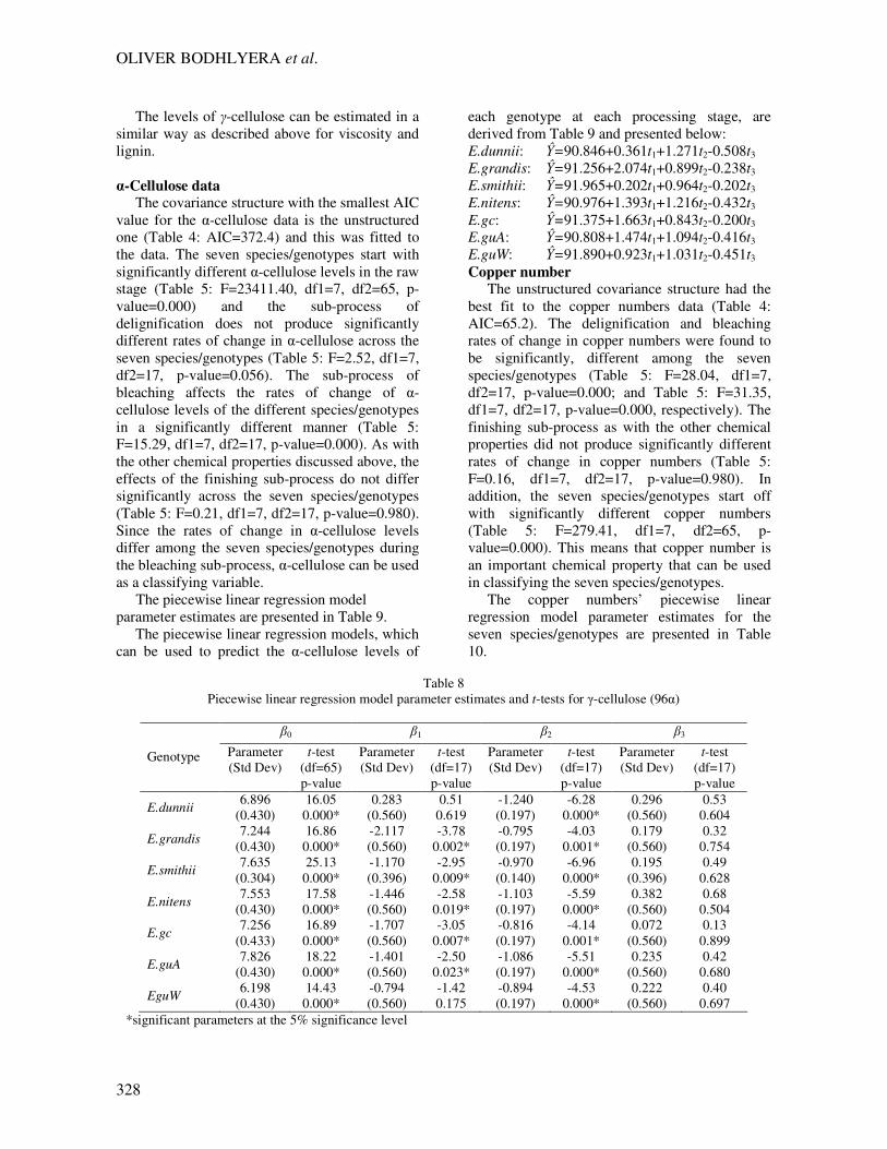
γ-Cellulose data For the γ-cellulose data, the unstructured

covariance structure had the lowest AIC value

(Table 4: AIC=284.9), hence it was used in the

analysis. As with viscosity and lignin, the

finishing stage had no significant effect on γ-cellulose (Table 5: F=0.21, df1=7, df2=17, p-

value=0.980). However, there were significant

differences in the changes in γ-cellulose levels

among the seven species/genotypes due to

delignification (Table 5: F=6.78, df1=7, df2=17,

p-value=0.001) and bleaching (Table 5: F=29.05,

df1=7, df2=17, p-value=0.000) sub-processes.

This means that γ-cellulose is an important

classifying variable for the seven

species/genotypes.

The piecewise linear regression model

parameters estimates for γ-cellulose are

summarized in Table 8. The results in Table 8

show that E.dunnii does not have a significant

reduction of γ-cellulose due to delignification

(Table 8: β1=0.283, t=0.51, df=17, p-

value=0.619). It is the only genotype that has this

behaviour out of the seven genotypes studied. The

other species/genotypes had significant reductions

in γ-cellulose levels during both delignification

and bleaching.

The corresponding piecewise linear regression

models derived from Table 8 for the seven

species/genotypes are as follows:

E.dunnii: Ŷ=6.896+0.283t1-1.240t2+0.296t3

E.grandis: Ŷ=7.244-2.117t1-0.795t2+0.179t3

E.smithii: Ŷ=7.635-1.170t1-0.970t2+0.195t3

E.nitens: Ŷ=7.553-1.466t1-1.103t2+0.382t3

E.gc: Ŷ=7.256-1.707t1-0.816t2+0.072t3

E.guA: Ŷ=7.826-1.401t1-1.086t2+0.235t3

E.guW: Ŷ=6.198-0.794t1-0.894t2+0.222t3


328

The levels of γ-cellulose can be estimated in a

similar way as described above for viscosity and

lignin.

α-Cellulose data The covariance structure with the smallest AIC

value for the α-cellulose data is the unstructured

one (Table 4: AIC=372.4) and this was fitted to

the data. The seven species/genotypes start with

significantly different α-cellulose levels in the raw

stage (Table 5: F=23411.40, df1=7, df2=65, p-

value=0.000) and the sub-process of

delignification does not produce significantly

different rates of change in α-cellulose across the

seven species/genotypes (Table 5: F=2.52, df1=7,

df2=17, p-value=0.056). The sub-process of

bleaching affects the rates of change of α-

cellulose levels of the different species/genotypes

in a significantly different manner (Table 5:

F=15.29, df1=7, df2=17, p-value=0.000). As with

the other chemical properties discussed above, the

effects of the finishing sub-process do not differ

significantly across the seven species/genotypes

(Table 5: F=0.21, df1=7, df2=17, p-value=0.980).

Since the rates of change in α-cellulose levels

differ among the seven species/genotypes during

the bleaching sub-process, α-cellulose can be used

as a classifying variable.


parameter estimates are presented in Table 9.

The piecewise linear regression models, which

can be used to predict the α-cellulose levels of

each genotype at each processing stage, are

derived from Table 9 and presented below:

E.dunnii: Ŷ=90.846+0.361t1+1.271t2-0.508t3

E.grandis: Ŷ=91.256+2.074t1+0.899t2-0.238t3

E.smithii: Ŷ=91.965+0.202t1+0.964t2-0.202t3

E.nitens: Ŷ=90.976+1.393t1+1.216t2-0.432t3

E.gc: Ŷ=91.375+1.663t1+0.843t2-0.200t3

E.guA: Ŷ=90.808+1.474t1+1.094t2-0.416t3

E.guW: Ŷ=91.890+0.923t1+1.031t2-0.451t3

Copper number The unstructured covariance structure had the

best fit to the copper numbers data (Table 4:

AIC=65.2). The delignification and bleaching

rates of change in copper numbers were found to

be significantly, different among the seven

species/genotypes (Table 5: F=28.04, df1=7,

df2=17, p-value=0.000; and Table 5: F=31.35,

df1=7, df2=17, p-value=0.000, respectively). The

finishing sub-process as with the other chemical

properties did not produce significantly different

rates of change in copper numbers (Table 5:

F=0.16, df1=7, df2=17, p-value=0.980). In

addition, the seven species/genotypes start off

with significantly different copper numbers

(Table 5: F=279.41, df1=7, df2=65, p-

value=0.000). This means that copper number is

an important chemical property that can be used

in classifying the seven species/genotypes.

The copper numbers’ piecewise linear

regression model parameter estimates for the

seven species/genotypes are presented in Table

10.

Table 8

Piecewise linear regression model parameter estimates and t-tests for γ-cellulose (96α)

β0 β1 β2 β3

Genotype Parameter

(Std Dev)

t-test

(df=65)

p-value

Parameter

(Std Dev)

t-test

(df=17)

p-value

Parameter

(Std Dev)

t-test

(df=17)

p-value

Parameter

(Std Dev)

t-test

(df=17)

p-value

E.dunnii 6.896

(0.430)

16.05

0.000*

0.283

(0.560)

0.51

0.619

-1.240

(0.197)

-6.28

0.000*

0.296

(0.560)

0.53

0.604

E.grandis 7.244

(0.430)

16.86

0.000*

-2.117

(0.560)

-3.78

0.002*

-0.795

(0.197)

-4.03

0.001*

0.179

(0.560)

0.32

0.754

E.smithii 7.635

(0.304)

25.13

0.000*

-1.170

(0.396)

-2.95

0.009*

-0.970

(0.140)

-6.96

0.000*

0.195

(0.396)

0.49

0.628

E.nitens 7.553

(0.430)

17.58

0.000*

-1.446

(0.560)

-2.58

0.019*

-1.103

(0.197)

-5.59

0.000*

0.382

(0.560)

0.68

0.504

E.gc 7.256

(0.433)

16.89

0.000*

-1.707

(0.560)

-3.05

0.007*

-0.816

(0.197)

-4.14

0.001*

0.072

(0.560)

0.13

0.899

E.guA 7.826

(0.430)

18.22

0.000*

-1.401

(0.560)

-2.50

0.023*

-1.086

(0.197)

-5.51

0.000*

0.235

(0.560)

0.42

0.680

EguW 6.198

(0.430)

14.43

0.000*

-0.794

(0.560)

-1.42

0.175

-0.894

(0.197)

-4.53

0.000*

0.222

(0.560)

0.40

0.697


Pulp

329

Table 9

Piecewise linear regression model parameter estimates and t-tests for α-cellulose (96α)

β0 β1 β2 β3

Genotype Parameter

(Std Dev)

t-test

(df=65)

p-value

Parameter

(Std Dev)

t-test

(df=17)

p-value

Parameter

(Std Dev)

t-test

(df=17)

p-value

Parameter

(Std Dev)

t-test

(df=17)

p-value

E.dunnii 90.846

(0.639)

142.28

0.000*

0.361

(0.833)

0.43

0.670

1.271

(0.286)

4.45

0.000*

-0.508

(0.833)

-0.61

0.550

E.grandis 91.256

(0.639)

142.92

0.000*

2.074

(0.833)

2.49

0.023*

0.899

(0.286)

3.15

0.006*

-0.238

(0.833)

-0.29

0.778

E.smithii 91.965

(0.452)

203.69

0.000*

0.202

(0.589)

0.34

0.735

0.964

(0.202)

4.77

0.000*

-0.202

(0.589)

-0.34

0.735

E.nitens 90.976

(0.639)

142.48

0.000*

1.393

(0.833)

1.67

0.113

1.216

(0.286)

4.26

0.001*

-0.432

(0.833)

-0.52

0.611

E.gc 91.375

(0.639)

143.11

0.000*

1.663

(0.833)

2.00

0.062

0.843

(0.286)

2.95

0.009*

-0.200

(0.833)

-0.24

0.813

E.guA 90.808

(0.639)

142.22

0.000*

1.474

(0.833)

1.77

0.095

1.094

(0.286)

3.83

0.001*

-0.416

(0.833)

-0.50

0.624

E.guW 91.890

(0.639)

143.91

0.000*

0.923

(0.833)

1.11

0.283

1.031

(0.286)

3.61

0.002*

-0.451

(0.833)

-0.54

0.595


Table 10

Piecewise linear regression model parameter estimates and t-tests for copper number (96α)

β0 β1 β2 β3

Genotype Parameter

(Std Dev)

t-test

(df=65)

p-value

Parameter

(Std Dev)

t-test

(df=17)

p-value

Parameter

(Std Dev)

t-test

(df=17)

p-value

Parameter

(Std Dev)

t-test

(df=17)

p-value

E.dunnii 3.107

(0.185)

16.83

0.000*

-1.064

(0.241)

-4.42

0.000*

-0.514

(0.083)

-6.22

0.000*

0.104

(0.241)

0.43

0.669

E.grandis 2.886

(0.185)

15.63

0.000*

-1.277

(0.241)

-5.30

0.000*

-0.414

(0.083)

-5.01

0.001*

0.083

(0.241)

0.34

0.736

E.smithii 2.974

(0.131)

22.78

0.000*

-1.245

(0.170)

-7.32

0.000*

-0.417

(0.058)

-7.14

0.000*

0.063

(0.170)

0.37

0.714

E.nitens 2.423

(0.185)

13.12

0.000*

-0.657

(0.241)

-2.73

0.014*

-0.452

(0.083)

-5.47

0.000*

0.105

(0.241)

0.44

0.669

E.gc 3.168

(0.185)

17.16

0.000*

-1.534

(0.241)

-6.37

0.000*

-0.418

(0.083)

-5.07

0.001*

0.075

(0.241)

0.31

0.759

E.guA 2.999

(0.185)

16.24

0.000*

-1.397

(0.241)

-5.80

0.000*

-0.410

(0.083)

-4.97

0.000*

0.102

(0.241)

0.42

0.678

E.guW 2.472

(0.430)

13.39

0.000*

-0.881

(0.241)

-3.66

0.002*

-0.408

(0.083)

-4.94

0.000*

0.112

(0.241)

0.47

0.647


All rates of change of copper numbers due to

delignification and bleaching are significant for

all species/genotypes (Table 10: all p-values for t-

test<0.05). From Table 10, the piecewise linear

regression models for copper numbers can be

constructed as:

E.dunnii: Ŷ=3.107-1.064t1-0.514t2+0.104t3

E.grandis: Ŷ=2.886-1.277t1-0.414t2+0.083t3

E.smithii: Ŷ=2.974-1.245t1-0.417t2+0.063t3

E.nitens: Ŷ=2.423-0.657t1-0.452t2+0.105t3

E.gc: Ŷ=3.168-1.534t1-0.418t2+0.075t3

E.guA: Ŷ=2.999-1.397t1-0.410t2+0.102t3

E.guW: Ŷ=2.472-0.881t1-0.408t2+0.112t3

The piecewise regression models can be used

to estimate copper numbers for the seven

species/genotypes at each stage by substituting

the values of t1, t2 and t3 that were described in

Table 2. The correlation between the percentage

of γ-cellulose at the beginning (raw pulp stage)

and at the end of processing was found to be

r=0.766. This means that there is a strong


330

relationship between the initial and final

percentage levels of γ-cellulose.

Glucose data

Having the lowest AIC value, the unstructured

covariance structure was fitted to the glucose data

(Table 4: AIC=276.5). The effects of

delignification and bleaching were significantly

different on the rates of change of glucose for the

seven species/genotypes (Table 5: F=38.01,

df1=7, df2=17, p-value=0.000; and Table 5:

F=41.01, df1=7, df2=17, p-value=0.000,

respectively). In general, glucose had significant

rates of change during delignification and

bleaching for all genotypes (Table 11: β1’s>0 and

β2’s>0 with p-values for t-tests<0.05 for all

genotypes). The changes in glucose due to the

finishing stage were not significant for all

species/genotypes.


parameter estimates derived from Table 11 are

shown below and these models can be used to

estimate glucose levels at each stage of chemical

processing using the values of t1, t2 and t3 defined

in Table 2 above.

E.dunnii: Ŷ=90.146+2.010t1+1.226t2-0.116t3

E.grandis: Ŷ=92.009+2.467t1+0.792t2-0.474t3

E.smithii: Ŷ=90.595+1.884t1+1.035t2-0.153t3

E.nitens: Ŷ=89.712+3.493t1+0.987t2-0.298t3

E.gc: Ŷ=89.619+3.640t1+0.701t2-0.054t3

E.guA: Ŷ=90.042+2.908t1+0.949t2-0.124t3

E.guW: Ŷ=92.454+2.493t1+0.675t2-0.672t3

Xylose data With the lowest AIC, the unstructured

covariance structure was of best fit to the xylose

data (Table 4: AIC=173.5). The rates of change in

xylose due to delignification and bleaching

differed significantly across the seven

species/genotypes (Table 5: F=14.01, df1=7,

df2=17, p-value=0.000; and Table 5: F=26.57,

df1=7, df2=17, p-value=0.000). This renders

xylose an important classification variable for the

seven species/genotypes. The finishing sub-

process, as with the other chemical properties, did

not have a significant effect on the final xylose

readings.

There were significant rates of decrease in

xylose during the delignification and bleaching

processes for most species/genotypes (Table 12:

β1’s<0, β2’s<0 with p-values<0.05 for t-tests),

except for EguA, which did not have a significant

decrease in xylose during delignification (Table

12: β1=-0.626, t=-1.95, df=17, p-value=0.068).

The finishing stage did not have a significant

effect on the xylose values just like with the other

chemical properties.

Table 11

Piecewise linear regression model parameter estimates and t-tests for Glucose (96α)

β0 β1 β2 β3

Genotype Parameter

(Std Dev)

t-test

(df=65)

p-value

Parameter

(Std Dev)

t-test

(df=17)

p-value

Parameter

(Std Dev)

t-test

(df=17)

p-value

Parameter

(Std Dev)

t-test

(df=17)

p-value

E.dunnii 90.146

(0.352)

256.46

0.000*

2.010

(0.461)

4.36

0.000*

1.226

(0.157)

7.80

0.000*

-0.116

(0.458)

-0.25

0.803

E.grandis 92.009

(0.352)

261.76

0.000*

2.467

(0.461)

5.35

0.000*

0.792

(0.157)

5.04

0.001*

-0.474

(0.458)

-1.03

0.315

E.smithii 90.595

(0.272)

332.74

0.000*

1.884

(0.345)

5.47

0.000*

1.035

(0.111)

9.31

0.000*

-0.152

(0.324)

-0.47

0.645

E.nitens 89.712

(0.352)

255.23

0.000*

3.493

(0.461)

7.57

0.014*

0.987

(0.157)

6.28

0.000*

-0.298

(0.458)

-0.65

0.524

E.gc 89.619

(0.352)

254.96

0.000*

3.640

(0.461)

7.89

0.000*

0.701

(0.157)

4.46

0.001*

0.054

(0.458)

0.12

0.908

E.guA 90.042

(0.352)

256.17

0.000*

2.908

(0.461)

6.30

0.000*

0.949

(0.157)

6.04

0.000*

0.124

(0.458)

0.27

0.791

EguW 92.454

(0.352)

263.03

0.000*

2.493

(0.461)

5.41

0.000*

0.675

(0.157)

4.29

0.001*

-0.672

(0.458)

-1.47

0.161


Pulp

331

Table 12

Piecewise linear regression model parameter estimates and t-tests for xylose (96α)

β0 β1 β2 β3

Genotype Parameter

(Std Dev)

t-test

(df=65)

p-value

Parameter

(Std Dev)

t-test

(df=17)

p-value

Parameter

(Std Dev)

t-test

(df=17)

p-value

Parameter

(Std Dev)

t-test

(df=17)

p-value

E.dunnii 4.714

(0.214)

22.04

0.000*

-0.857

(0.322)

-2.66

0.016*

-0.565

(0.096)

-5.91

0.000*

-0.037

(0.279)

-0.13

0.895

E.grandis 3.367

(0.214)

15.75

0.000*

-0.545

(0.322)

-1.69

0.109*

-0.402

(0.096)

-4.21

0.001*

0.084

(0.279)

0.30

0.766

E.smithii 4.912

(0.166)

29.66

0.000*

-1.032

(0.237)

-4.35

0.000*

-0.528

(0.068)

-7.80

0.000*

0.069

(0.197)

0.35

0.729

E.nitens 5.939

(0.214)

27.77

0.000*

-2.279

(0.322)

-7.09

0.000*

-0.484

(0.096)

-5.06

0.000*

0.017

(0.279)

0.06

0.952

E.gc 3.927

(0.214)

18.37

0.000*

-0.817

(0.322)

-2.54

0.021*

-0.291

(0.096)

-3.04

0.007*

0.218

(0.279)

0.78

0.445

E.guA 4.340

(0.214)

20.29

0.000*

-0.626

(0.322)

-1.95

0.068

-0.516

(0.096)

-5.39

0.000*

-0.046

(0.279)

-0.16

0.871

E.guW 3.244

(0.214)

15.17

0.000*

-0.951

(0.322)

-2.96

0.009*

-0.280

(0.096)

-2.93

0.009*

0.055

(0.279)

0.20

0.846


The parameter estimates for the piecewise

linear regression models for xylose derived from

Table 12 are presented below:

E.dunnii: Ŷ=4.714-0.857t1-0.565t2-0.037t3

E.grandis: Ŷ=3.367-0.545t1-0.402t2+0.084t3

E.smithii: Ŷ=4.912-1.032t1-0.528t2+0.069t3

E.nitens: Ŷ=5.939-2.279t1-0.484t2+0.017t3

E.gc: Ŷ=3.927-0.817t1-0.291t2+0.218t3

E.guA: Ŷ=4.340-0.626t1-0.516t2-0.046t3

E.guW: Ŷ=3.244-0.951t1-0.280t2+0.055t3

Although some parameter estimates for the

finishing sub-process are negative, most of them

are generally positive. It was observed that for all

chemical properties, the finishing stage had the

general effect of reversing the trend in bleaching,

but such reversal is not significant. Glucose is

also an important classifying variable for the

seven species/genotypes.

CONCLUSION The piecewise linear regression models had

the capability of outlining the effect of each sub-

process of chemical pulping on the seven

reactivity variables studied. The ability of the

model to state, by the model parameters, the

effect of each sub-process on the chemical

properties is a value addition to the study of

chemical pulping processes. This can be extended

to other types of pulp processing with known sub-

processes i.e. kraft pulping, neutral sulphite

pulping.

Based on the results from the piecewise linear

regression models, it was established that the six

chemical properties lignin, γ-cellulose, α-

cellulose, copper numbers, glucose and xylose

were important classification variables for

species/genotypes, while viscosity, based on the

results obtained, was not. This means that when

one wants to compare or group wood

species/genotypes using their chemical properties

for the purpose of deciding which ones are

mixable during processing, they do not need to

consider viscosity.

Using the coding of the stages as shown in

Table 2, the levels of the chemical properties

studied can be estimated at each stage using the

piecewise linear regression models developed in

this study. This is essential to dissolving pulp

manufacturers as the model can be used as a

predictive tool to assess species/genotype

properties without having to carry out the actual

bleaching, especially if such models have already

been developed for the concerned timber

species/genotype. This will reduce the use of

costly chemicals, as well as limit the generation of

harmful waste. Another advantage of the

developed models is that the parameter estimates

for the various species/genotypes can be grouped

according to their sizes in order to classify the


332

species/genotypes into groups of mixable species

or genotypes during chemical processing. This

reduces the trial and error involved in selecting

specific clones and species for specific grades of

dissolving pulp. The methodology can thus be

used for other pulps earmarked for other products

in the timber industry.

For further studies, it would of interest to

develop a classifying method based on

multivariate statistical techniques, such as cluster

analysis, classification algorithms and stepwise

linear regression.

ACKNOWLEDGMENTS: The Council for

Scientific and Industrial Research (CSIR) and

Sappi Saiccor of South Africa are acknowledged

for, in part, financially supporting the project. The

Forestry and Forest Products Research Centre,

CSIR-Durban, where the pulping, bleaching and

data generation work was conducted, also

deserves special acknowledgement.

REFERENCES 1

M. S. Jahan, L. Ahsan, A. Noori and M. A.

Quaiyyum, Bioresources, 3, 816 (2008) 2

J. F. Hinck, R. L. Casabier and J. K. Hamilton,

“Sulphite Science and Technology”, Joint Textbook

Committee of Paper Industry, Atlanta, 1985, pp. 213-

242. 3

M. Sharma, R. N. Shukla, IJERT, 2, 1 (2013). 4 C. J. Biermann, “Handbook of Pulping and

Papermaking”, Academic Press, San Diego, 1993, p.

72. 5

J. C. Roberts, “The Chemistry of Paper”, The Royal

Society of Chemistry, Letchworth (UK), 1996, p. 9. 6

H. Karlsson, “Fibre Guide – Fibre Analysis and

Process Applications in the Pulp and Paper Industry”,

AB Lorentzen & Wettre, Sweden, 2006. 7 J. Gierer, Wood Sci. Technol., 19, 289 (1985). 8

M. Funaoka, V. L. Chang, K. Kolppo, D. D. Stokke,

Bull. Fac. Bioresources, Mie Univ., 5, 37 (1991). 9

D. W. Sundstrom, H. E. Klel and T. H. Daubenspeck,

Ind. Eng. Chem. Prod. Res. Dev., 22, 496 (1983). 10

J. P. Casey, “Pulp and Paper, Chemisty and

Chemical Technology”, Vol. 4, 3rd

ed., John Wiley &

Sons, Toronto, 1983. 11 Alkali solubility of pulp, Tappi T235 OM- 60, Tappi

Press, Atlanta, 2000. 12

Viscosity of pulp, Tappi T230 om-94, Tappi Press,

Atlanta, 2013. 13 Permanganate number of pulp, Tappi UM251, Tappi

Press, Atlanta, 2013. 14

J. Röhrling, A. Potthast, T. Rosenau, T. Lange, G.

Ebner et al., Biomacromolecules, 3, 959 (2002). 15 P. R. R. Wallajapet, R. T. Shet, “Copper number of

pulp, paper and paperboard”, Tappi T430 OM 94,

Tappi Press, Atlanta, 1998.

16 M. W. Davis, J. Wood Chem. Technol., 18, 235

(1998). 17

K. A. Bollen and P. J. Curran, “Latent Curve

Models: A Structural Equation Perspective”, Wiley

Series in Probability and Mathematical Statistics, New

York, 2006, pp. 103. 18

G. M. Fitzmaurice, N. M Laird and J. H. Ware,

“Applied Longitudinal Analysis”, Wiley Series in

Probability and Mathematical Statistics, New Jersey,

2004, pp. 147. 19

H. Bozdogan, Psychometrica, 52, 345 (1987). 20

R. C. Littell, G. A. Milliken, W. W. Stroup, R. D.

Wolfinger and O. Schabenberger, “SAS for Mixed

Models” ,2nd Ed., SAS Institute Inc., 2006, pp. 717. 21

L. Dechateau, P. Jansen and G. J. Rowlands, “Linear

Models. An Introduction with Applications in

Veterinary Reserarch”, International Livestock

Research Institute, Kenya, 1998, pp. 23.

ANALYSIS OF THE CHANGES IN CHEMICAL …2015)/p.317-332.pdf · ANALYSIS OF THE CHANGES IN CHEMICAL...

Documents

Transcript of ANALYSIS OF THE CHANGES IN CHEMICAL …2015)/p.317-332.pdf · ANALYSIS OF THE CHANGES IN CHEMICAL...