Analysis of Tensegrity Structures Using Abaqus
36
Georgia Southern University Georgia Southern University Digital Commons@Georgia Southern Digital Commons@Georgia Southern Honors College Theses 2018 Analysis of Tensegrity Structures Using Abaqus Analysis of Tensegrity Structures Using Abaqus Kayla M. Allen Georgia Southern University Follow this and additional works at: https://digitalcommons.georgiasouthern.edu/honors-theses Part of the Civil Engineering Commons, and the Structural Engineering Commons Recommended Citation Recommended Citation Allen, Kayla M., "Analysis of Tensegrity Structures Using Abaqus" (2018). Honors College Theses. 553. https://digitalcommons.georgiasouthern.edu/honors-theses/553 This thesis (open access) is brought to you for free and open access by Digital Commons@Georgia Southern. It has been accepted for inclusion in Honors College Theses by an authorized administrator of Digital Commons@Georgia Southern. For more information, please contact [email protected].
Transcript of Analysis of Tensegrity Structures Using Abaqus

Georgia Southern University Georgia Southern University
Digital Commons@Georgia Southern Digital Commons@Georgia Southern
Honors College Theses
2018
Analysis of Tensegrity Structures Using Abaqus Analysis of Tensegrity Structures Using Abaqus
Kayla M. Allen Georgia Southern University
Follow this and additional works at: https://digitalcommons.georgiasouthern.edu/honors-theses
Part of the Civil Engineering Commons, and the Structural Engineering Commons
Recommended Citation Recommended Citation Allen, Kayla M., "Analysis of Tensegrity Structures Using Abaqus" (2018). Honors College Theses. 553. https://digitalcommons.georgiasouthern.edu/honors-theses/553
This thesis (open access) is brought to you for free and open access by Digital Commons@Georgia Southern. It has been accepted for inclusion in Honors College Theses by an authorized administrator of Digital Commons@Georgia Southern. For more information, please contact [email protected].

Analysis of Tensegrity Structures Using Abaqus
An Honors Thesis submitted in partial fulfillment of the requirements for Honors in the
Department of Civil Engineering and Construction.
By
Kayla Marie Allen
Under the mentorship of Dr. Shahnam Navaee and Dr. Gustavo Maldonado
ABSTRACT
This project involves modeling and analysis of a tensegrity structure using the finite
element approach utilizing Abaqus. A tensegrity structure is a special type of assembly
consisting of a series of straight solid members, arranged in various geometrical
configurations in three-dimensional space and held together by series of cables. A web
search for this type of structure yields a variety of structural components ranging from a
simple frame in the shape of a table, supporting a flat top platform with three straight
members and six cables, to a more innovative architectural bridge structure with large
number of members and cables. Other examples of a tensegrity structure include a variety
of load-bearing and non-load bearing sculptures and arches with a large number of
component parts arranged in various intriguing configurations. The developed FE models
for several tensegrity structures are included in this presentation to better describe the
project.
Thesis Mentors:________________________
Dr. Shahnam Navaee
________________________
Dr. Gustavo Maldonado
Honors Director:_______________________
Dr. Steven Engel
April 2018
Department of Civil Engineering and Construction
University Honors Program
Georgia Southern University

Introduction
Engineering is a field that makes full use of technological advances and advances
in design. This is a field that is always evolving based on the evolution of technology and
the ability for computers to quickly process data and information that would take much
longer by hand. This study incorporates the use of advances in both design and
technology in the field of engineering.
One program now used in engineering is Abaqus CAE, which is a software
program used to visualize finite element analyses. In this software it is possible to model,
analyze, manage jobs, and visualize results of any geometry that is created in the program
[1]. It is possible to import CAD (Computer Aided Design) files into the software to
create models, as well as design models directly in the program [2]. For the purposes of
this study it was chosen to create all the models in the program itself. Abaqus is able to
run accurate analysis of stresses, strains and other mechanical properties without repeated
testing in real life which ca be time consuming and costly.
Engineering also highly values structures that are both aesthetically pleasing and
functional in use. A structure that embodies these characteristics would be a tensegrity
structure. Tensegrity structures combine a pleasing aesthetic with a lightweight design
[3]. They are a structure that is formed using a system of cables that are in tension and
rods in compression. Despite the members of the structure being joined with pin-type
connections the structure is rigid because there is equilibrium within all the parts [4].
Tensegrity structures have a light self-weight which means that they are ideal for large
span structures and other cases where there needs to be minimal addition of load as a
result of weight from the structure itself [5]. These characteristics make tensegrity

structures ideal for use in design as they can be intricately detailed in design, but are also
able to withstand loads applied to them allowing for them to be used as support.
This research investigates the process of analyzing a tensegrity structure modeled
in Abaqus. It looks to find the correct steps and procedure to properly model the members
and connections in order to have the model simulate that of a tensegrity structure. This is
done in order to easily analyze the resulting forces and stresses acting in the members
once a load is applied and the structure reaches equilibrium. This process should allow
for visualization of the results in the members after application of the load. The means,
methods and results of this process are presented here.
Methodology
In this project, analysis of tensegrity structures utilizing the Abaqus software
package is outlined and discussed. Abaqus is a comprehensive and sophisticated software
tool used in prestigious engineering schools and premiere engineering research facilities
worldwide to solve complex engineering problems. Through the course of investigations
conducted in this applied research project, a variety of approaches and techniques were
explored to develop a correct model that can accurately determine the behavior of a
tensegrity structure under statically applied loads.
The procedure developed in undertaking this project can be applied to analyze a
variety of other more complex three-dimensional structures, connected in various ways,
and subjected to various static and dynamic loads. The effects of geometric nonlinearity
and material nonlinearity can also be incorporated in the produced models using more
advanced features and tools in Abaqus to further enhance the utility of the developed
models. Some of these capabilities were explored in various online resources [6-8].
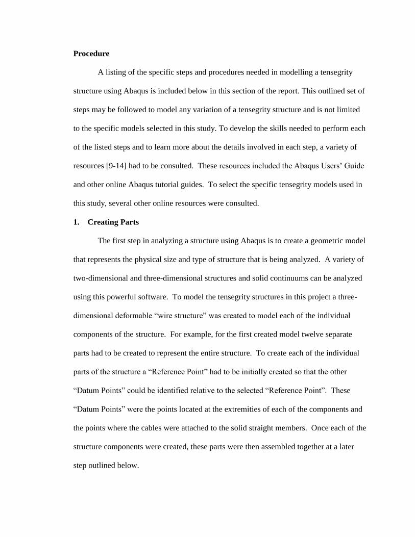
Procedure
A listing of the specific steps and procedures needed in modelling a tensegrity
structure using Abaqus is included below in this section of the report. This outlined set of
steps may be followed to model any variation of a tensegrity structure and is not limited
to the specific models selected in this study. To develop the skills needed to perform each
of the listed steps and to learn more about the details involved in each step, a variety of
resources [9-14] had to be consulted. These resources included the Abaqus Users’ Guide
and other online Abaqus tutorial guides. To select the specific tensegrity models used in
this study, several other online resources were consulted.
1. Creating Parts
The first step in analyzing a structure using Abaqus is to create a geometric model
that represents the physical size and type of structure that is being analyzed. A variety of
two-dimensional and three-dimensional structures and solid continuums can be analyzed
using this powerful software. To model the tensegrity structures in this project a three-
dimensional deformable “wire structure” was created to model each of the individual
components of the structure. For example, for the first created model twelve separate
parts had to be created to represent the entire structure. To create each of the individual
parts of the structure a “Reference Point” had to be initially created so that the other
“Datum Points” could be identified relative to the selected “Reference Point”. These
“Datum Points” were the points located at the extremities of each of the components and
the points where the cables were attached to the solid straight members. Once each of the
structure components were created, these parts were then assembled together at a later
step outlined below.

2. Defining Material
Once the members of the structures are created, the material properties for each
component should be specified. These properties are essentially related to the type of
material selected. For the tensegrity structures selected for this project. A structural Steel
(A-36 Steel) with the following material properties were used: E = 29 x 106 psi and n =
0.32. The E and n are respectively the “Modulus of Elasticity” and “Poisson Ratio” for
the material. These material constants basically determine how the members will deform
when subjected to loads.
3. Creating Cross-Section Profiles
In this step of the procedure, the geometric shape and the dimensions of the cross-
section for each of the structure members should be defined. In this project, a hollow
circular tube with an outside radius of r = 5/16 in. and thickness of t = 1/8 in. were
selected for the compression members. For the tension cables, a solid circular cross-
section of radius r = 1/16 in. was chosen.
4. Creating Sections
Next, the created material properties and member profiles have to be assigned to
each member of the structure. In this project two sections were created, one for
compression tube members, and the other for tension cables.
5. Assigning Sections to Members
Once the “Sections” are generated as described in the previous step, these sections
need to be assigned to various members of the structures, so that Abaqus can accurately
determine the behavior of the structure.
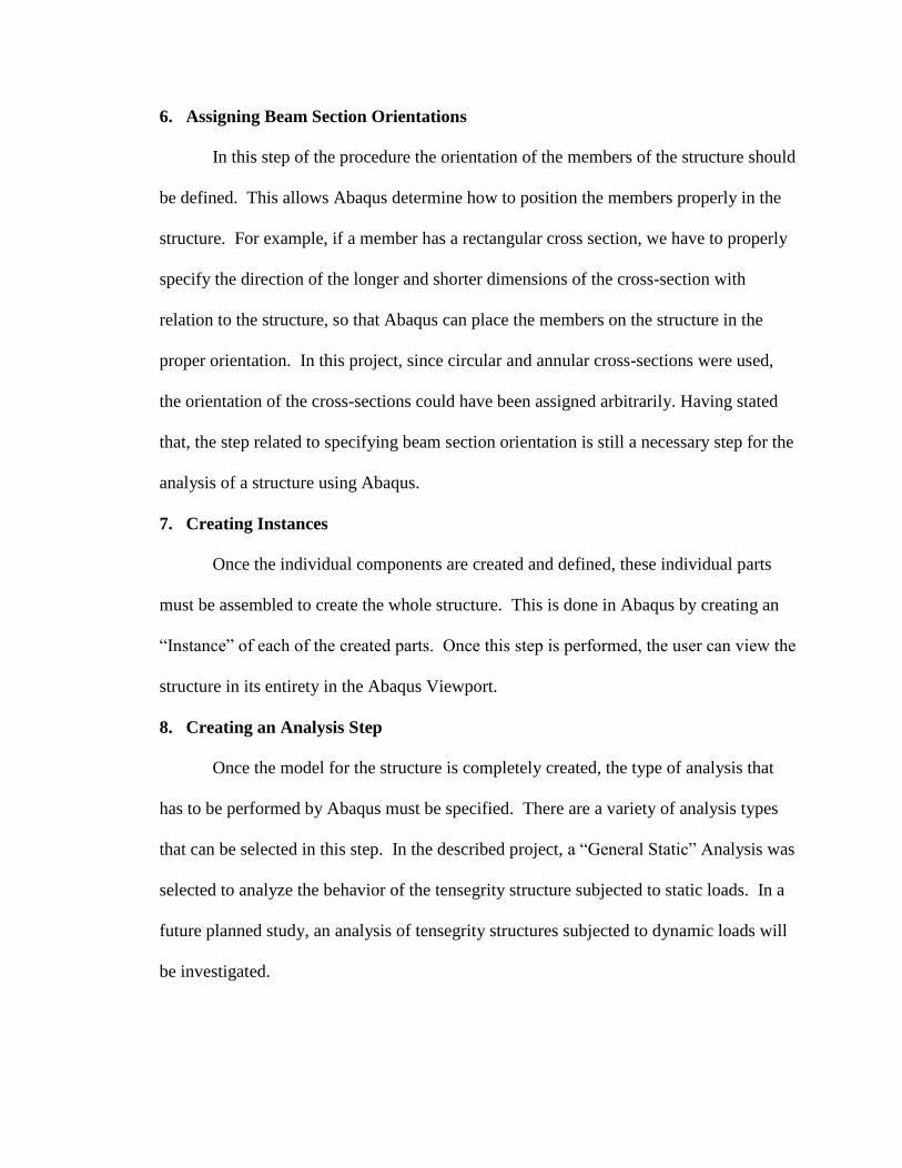
6. Assigning Beam Section Orientations
In this step of the procedure the orientation of the members of the structure should
be defined. This allows Abaqus determine how to position the members properly in the
structure. For example, if a member has a rectangular cross section, we have to properly
specify the direction of the longer and shorter dimensions of the cross-section with
relation to the structure, so that Abaqus can place the members on the structure in the
proper orientation. In this project, since circular and annular cross-sections were used,
the orientation of the cross-sections could have been assigned arbitrarily. Having stated
that, the step related to specifying beam section orientation is still a necessary step for the
analysis of a structure using Abaqus.
7. Creating Instances
Once the individual components are created and defined, these individual parts
must be assembled to create the whole structure. This is done in Abaqus by creating an
“Instance” of each of the created parts. Once this step is performed, the user can view the
structure in its entirety in the Abaqus Viewport.
8. Creating an Analysis Step
Once the model for the structure is completely created, the type of analysis that
has to be performed by Abaqus must be specified. There are a variety of analysis types
that can be selected in this step. In the described project, a “General Static” Analysis was
selected to analyze the behavior of the tensegrity structure subjected to static loads. In a
future planned study, an analysis of tensegrity structures subjected to dynamic loads will
be investigated.
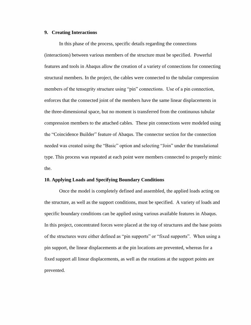
9. Creating Interactions
In this phase of the process, specific details regarding the connections
(interactions) between various members of the structure must be specified. Powerful
features and tools in Abaqus allow the creation of a variety of connections for connecting
structural members. In the project, the cables were connected to the tubular compression
members of the tensegrity structure using “pin” connections. Use of a pin connection,
enforces that the connected joint of the members have the same linear displacements in
the three-dimensional space, but no moment is transferred from the continuous tubular
compression members to the attached cables. These pin connections were modeled using
the “Coincidence Builder” feature of Abaqus. The connector section for the connection
needed was created using the “Basic” option and selecting “Join” under the translational
type. This process was repeated at each point were members connected to properly mimic
the.
10. Applying Loads and Specifying Boundary Conditions
Once the model is completely defined and assembled, the applied loads acting on
the structure, as well as the support conditions, must be specified. A variety of loads and
specific boundary conditions can be applied using various available features in Abaqus.
In this project, concentrated forces were placed at the top of structures and the base points
of the structures were either defined as “pin supports” or “fixed supports”. When using a
pin support, the linear displacements at the pin locations are prevented, whereas for a
fixed support all linear displacements, as well as the rotations at the support points are
prevented.

11. Seeding the Model
To perform the finite element analysis of the structure, it is necessary to first
“Seed” each member of the structure. By seeding the members, we basically divide each
component of the structure into “Finite Element” pieces that can be analyzed using
Abaqus. The number of elements chosen for the analysis can be defined by the user and
can vary based on the specific problem analyzed. In general, to obtain more accurate
results it is best to use more elements. For the models presented in this report five
elements were used for each unsupported length of the members. More element can be
chosen if needed.
12. Meshing the Model
Once the structure is seeded, it has be “Meshed” by selecting an appropriate
element type. In general, there are variety of elements that can be selected for various
structures and solids. These include: truss elements, beam elements, shell elements, and
continuum elements. For the structures analyzed in this project a linear beam element
was selected (B31 Element: A 2-node linear beam in space).
13. Creating and Running the Program
Once all steps outlined above are completed, an analysis job can then be created
and submitted to produce the needed results. This output can visually be displayed in a
variety of forms on the computer screen, and tabulated in a written report in any desired
format. Sample screenshots of Abaqus’ Viewport showing the deflected shapes of the
models analyzed in this project are provided in Figures. 1-5. Also, a sample produced
report showing the analysis results for one of the studied models (Model 1) is provided in
Appendix B. These results include the reaction forces at the structure supports, and the

displacements and axial stresses at several defined nodal points along the length of each
member of the structure.
Produced Models
As mentioned previously, a total of five tensegrity structures were modeled in this
project. All structures were assumed to be structural steel (A-36 Steel) with the
following material properties: E = 29 x 106 psi and n = 0.32. The E and n are
respectively the “Modulus of Elasticity” and “Poisson Ratio” for the material. These
material properties determine how the structure will deform when subjected to loads. All
compression members used in the models were selected as tubes with an outside radius of
5/16 in. and a thickness of 1/8 in. The tension cables incorporated assumed to have a
circular cross-section with a radius of 1/16 in. To be able to analyze the behavior of each
segment of all models studied in this project, six nodal points were used to divide each
segment of the structure into five elements. This discretization is necessary in the analysis
of the problem when using the finite element approach. These nodal points can be seen in
Figures. 1(b) through Figure. 5(b). As previously stated, more modal points (or
elements) can be used if desired.
Model 1
Model 1 was created using Abaqus for the first tensegrity structure analyzed in
the project. Figure 1(a) shows the undeformed structure and the loading, while Figure
1(b) illustrates the deformed configuration of the structure, including the nodal points
used in the analysis of the problem. This model had twelve members, 3 tubular rods
(compression members), and nine cables (tension members). The total length of each rod
used in the structure was 28 in. and the connection points of the cables to the rods were 2
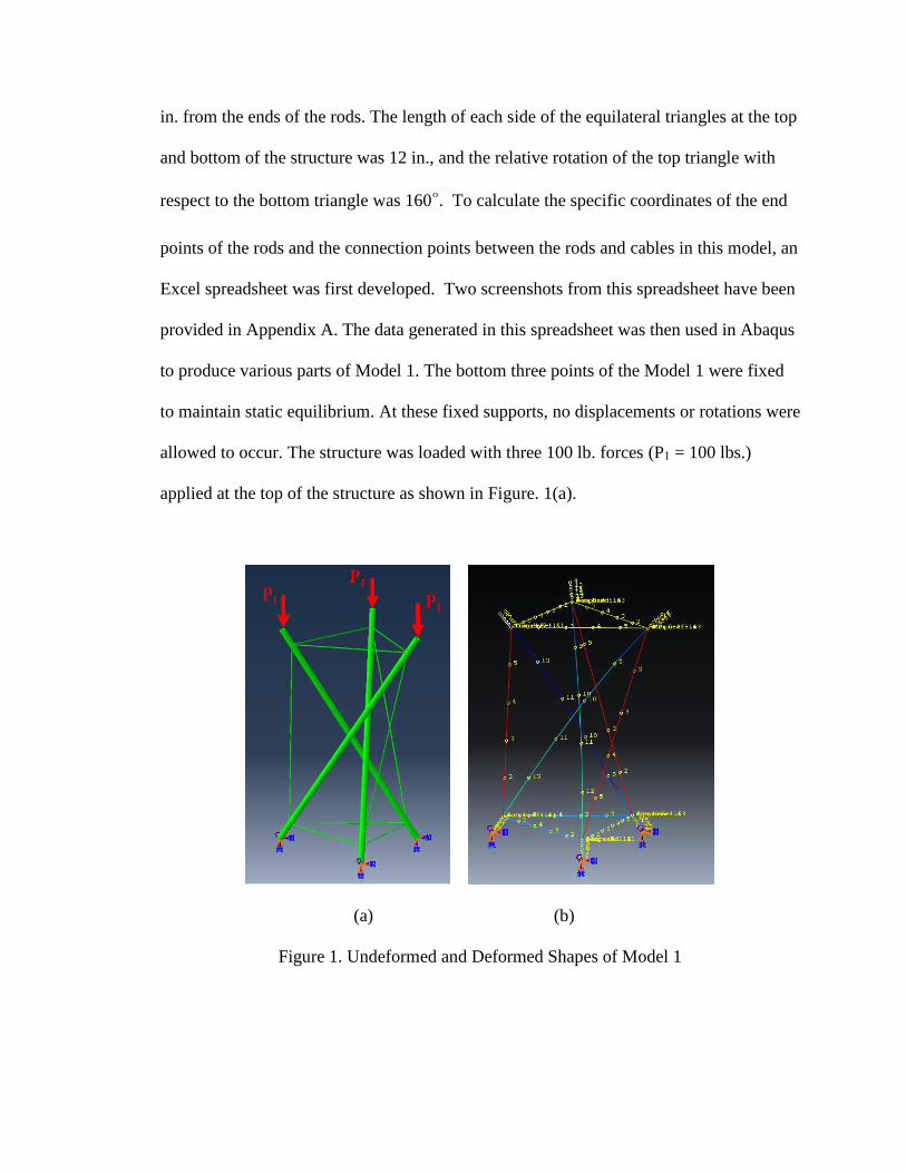
in. from the ends of the rods. The length of each side of the equilateral triangles at the top
and bottom of the structure was 12 in., and the relative rotation of the top triangle with
respect to the bottom triangle was 160°. To calculate the specific coordinates of the end
points of the rods and the connection points between the rods and cables in this model, an
Excel spreadsheet was first developed. Two screenshots from this spreadsheet have been
provided in Appendix A. The data generated in this spreadsheet was then used in Abaqus
to produce various parts of Model 1. The bottom three points of the Model 1 were fixed
to maintain static equilibrium. At these fixed supports, no displacements or rotations were
allowed to occur. The structure was loaded with three 100 lb. forces (P1 = 100 lbs.)
applied at the top of the structure as shown in Figure. 1(a).
(a) (b)
Figure 1. Undeformed and Deformed Shapes of Model 1

Model 2
Model 2 closely resembled Model 1, however, the total length of the rods was 24
in. and the cables were connected to the rods at the end points of the rods. This model
also had twelve members, three rods (in compression), and nine cables (in tension).
Rather than “fixed supports”, three “pin supports” were used at the bottom of this model
to support the structure. These pins allowed rotations to occur at the base supports, but
no displacements. Similar to Model 1, again three 100 lb. vertical forces (P1 = 100 lbs.)
were applied to the top three points of the structure.
(a) (b)
Figure 2. Undeformed and Deformed Shapes of Model 2
Model 3
In Model 3, two horizontal equilateral triangle bases were used at the bottom and
top of the structure. There was no relative rotation between the top and bottom triangles.
The length of each side of the bottom and top equilateral triangles were respectively 12

in. and 6 in. The model consisted of twelve members, six rods in compression, and six
cables in tension. The model was supported by three pins at the bottom and was
subjected to three vertical loads of 100 lb. each (P1 = 100 lbs.), and three horizontal
loadings of 20 lbs. (P2 = 20 lbs.). These loads are shown in Figure. 3(a).
(a) (b)
Figure 3. Undeformed and Deformed Shapes of Model 3
Model 4
Model 4 had square bases at the bottom and top, and consisted of sixteen members (four
compression rods, and twelve tension cables). The length of each square side was 12 in.
and the diagonal members used in the structure had a length of 24 in. The structure was
supported by four pins at the bottom and was subjected to four vertical loads of 100 lbs.
each (P1 = 100 lbs.), and four additional horizontal loadings of 20 lb. (P2 = 20 lbs.).
These loads can be seen in Figure. 4(a).

(a) (b)
Figure 4. Undeformed and Deformed Shapes of Model 4
Model 5
The final model analyzed in this project, Model 5, consisted of two rectangular
bases, one at the top and one at the bottom. The dimensions of the bottom and top
rectangles were respectively 144 in. x 96 in., and 72 in. x 48 in. The top rectangle was
placed symmetrically above the bottom rectangle without any relative angular rotation.
This model has similarity to a problem included in reference [15].
Similar to the previous three models analyzed in this study, this structure also had
pin supports at the bottom to prevent any displacements at the supports. The structure
was subjected to four vertical loads of 100 lbs. each (P1 = 100 lbs.) and four horizontal
loads of magnitude 50 lbs. (P3 = 50 lbs.). The directions of these forces are shown in
Figure. 5(a). This model had seventeen members, and due to the applied loading eight
tubular members experienced compression, and the remaining nine cable members were
in tension.

(a) (b)
Figure 5. Undeformed and Deformed Shapes of Model 5
Results
The tabulated results of the analyses performed in Abaqus can be created by using
the “Field Output Request” feature of Abaqus. When using this feature, one can specify
the type of output desired to be generated. Partial results created using Abaqus for the
five models studied in this project are provided in Tables 1 -10. These results include the
reactions at the supports of the structures, and the displacements at the ends of the
compression rods. For Model 1, the displacements of the connection points between the
rods and cables were also provided. Sample tabulated reports created in Abaqus showing
the complete set of results for Model 1 is provided in Appendix B. These results include
the support reactions, as well as the displacements, rotations, and axial stresses at
specified nodal points along the length of each member of the structure.
For each of the models, various checks were made to make sure that the structures
were analyzed correctly. For example, the reactions at the supports of the structures in

the x, y, and z directions were totaled to makes sure these results equaled the applied
loads in the corresponding directions. This was done to ensure that the structures were
indeed in static equilibrium. Additionally, the displacements at the connecting nodes of
various parts were checked to make certain that these nodes were displaced by the same
amount to ensure required deformation compatibility.
Figure 6. Undeformed Shape of Model 1 with Node Labels
Table 1. Reaction Forces at Lower End Nodes for Model 1
Node label Reaction Force in
x-direction (lbs.)
Reaction Forces in
y-direction (lbs.)
Reaction Forces in
z-direction (lbs.)
1 -79.58 51.71 100.00
2 -4.98 -94.77 100.00
3 84.56 43.06 100.00
7
4
1
2
3
5
6 8
9
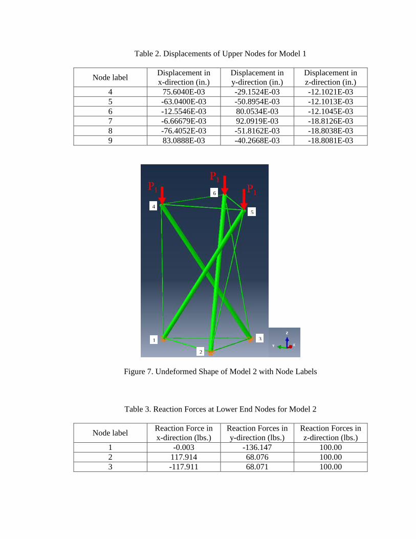
Table 2. Displacements of Upper Nodes for Model 1
Node label Displacement in
x-direction (in.)
Displacement in
y-direction (in.)
Displacement in
z-direction (in.)
4 75.6040E-03 -29.1524E-03 -12.1021E-03
5 -63.0400E-03 -50.8954E-03 -12.1013E-03
6 -12.5546E-03 80.0534E-03 -12.1045E-03
7 -6.66679E-03 92.0919E-03 -18.8126E-03
8 -76.4052E-03 -51.8162E-03 -18.8038E-03
9 83.0888E-03 -40.2668E-03 -18.8081E-03
Figure 7. Undeformed Shape of Model 2 with Node Labels
Table 3. Reaction Forces at Lower End Nodes for Model 2
Node label Reaction Force in
x-direction (lbs.)
Reaction Forces in
y-direction (lbs.)
Reaction Forces in
z-direction (lbs.)
1 -0.003 -136.147 100.00
2 117.914 68.076 100.00
3 -117.911 68.071 100.00
4
1
2
3
5
6

Table 4. Displacements of Upper Nodes for Model 2
Node label Displacement in
x-direction (in.)
Displacement in
y-direction (in.)
Displacement in
z-direction (in.)
4 -67.1168E-03 -54.3193E-03 -12.7346E-03
5 80.6062E-03 -30.9712E-03 -12.7355E-03
6 -13.4823E-03 85.2951E-03 -12.7373E-03
Figure 8. Undeformed Shape of Model 3 with Node Labels
Table 5. Reaction Forces at Lower End Nodes for Model 3
Node label Reaction Force in
x-direction (lbs.)
Reaction Forces in
y-direction (lbs.)
Reaction Forces in
z-direction (lbs.)
1 2.886 -17.284 142.689
2 -0.909 6.142 78.6557
3 -1.977 -8.858 78.6557
4
1
2
3
5
6

Table 6. Displacements of Upper Nodes for Model 3
Node label Displacement in
x-direction (in.)
Displacement in
y-direction (in.)
Displacement in
z-direction (in.)
4 -14.5872E-03 3.78238E-03 -71.8001E-06
5 7.31666E-03 -8.86727E-03 -787.269E-06
6 7.29499E-03 16.4555E-03 -874.562E-06
Figure 9. Undeformed Shape of Model 4 with Node Labels
Table 7. Reaction Forces at Lower End Nodes for Model 4
Node label Reaction Force in
x-direction (lbs.)
Reaction Forces in
y-direction (lbs.)
Reaction Forces in
z-direction (lbs.)
1 0.00 -20 .00 100.00
2 20 .00 0.00 100.00
3 -0.00 20.00 100.00
4 -20.00 0.00 100.00
1
2
3
4
8
7
6
5
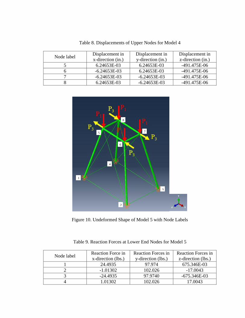
Table 8. Displacements of Upper Nodes for Model 4
Node label Displacement in
x-direction (in.)
Displacement in
y-direction (in.)
Displacement in
z-direction (in.)
5 6.24653E-03 6.24653E-03 -491.475E-06
6 -6.24653E-03 6.24653E-03 -491.475E-06
7 -6.24653E-03 -6.24653E-03 -491.475E-06
8 6.24653E-03 -6.24653E-03 -491.475E-06
Figure 10. Undeformed Shape of Model 5 with Node Labels
Table 9. Reaction Forces at Lower End Nodes for Model 5
Node label Reaction Force in
x-direction (lbs.)
Reaction Forces in
y-direction (lbs.)
Reaction Forces in
z-direction (lbs.)
1 24.4935 97.974 675.346E-03
2 -1.01302 102.026 -17.0043
3 -24.4935 97.9740 -675.346E-03
4 1.01302 102.026 17.0043
1
8
7
6
5
4
3
2

Table 10. Displacements of Upper Nodes for Model 5
Node label Displacement in
x-direction (in.)
Displacement in
y-direction (in.)
Displacement in
z-direction (in.)
5 -44.0400E-03 -2.14898E-03 -53.2180E-03
6 -44.3433E-03 -6.58723E-03 53.0775E-03
7 44.0400E-03 -2.14898E-03 53.2180E-03
8 44.3433E-03 -6.58723E-03 -53.0775E-03
Conclusions and Future Research Plans
In this research a procedure for analyzing a tensegrity structure using the Abaqus
software package was outlined and discussed. The models and analyses results for five
developed tensegrity structures were included in the report to further illustrate the details
related to the developed procedure and the structures analyzed. In developing these
models, each part of the structure was created as a separate piece. This was purposely
done in order to make the developed models more flexible. In these models the material
and geometric properties of each of the parts can easily be modified to obtain the solution
for a variety of other structures. Based on the performed study, a poster has been
prepared for presentation at the 2018 CEIT Student Research Symposium on April 19th.
The mentors of this project are also planning to submit a paper based on the performed
research to the 2019 American Society for Engineering Education (ASEE) Annual
Conference. The research performed in the study has been successful in the sense that
this study has laid the foundation for conducting other future studies related to the
analysis of structures subjected to more complicated loadings and material conditions.
Some of these cases include the following class of problems: (a) large deformations of
structural members, (b) study of structures exhibiting nonlinear material behavior, and (c)
dynamic loadings of structures. When solving any nonlinear problem, an iterative

procedure should be employed through which the loads are applied to the structure in
small increments. Convergence of results is needed in each load increment, before the
next increment of load can be applied. The process is continued until the total load is
applied in full. This iterative process can require a significant amount of computational
effort. The Abaqus software contains powerful features which can handle nonlinear
problems. The mentors of this study are planning to conduct future research related to the
above mentioned classes of problems.
References
[1] “Abaqus (Finite Element Analysis & Multiphysics Simulation),” feasol.com.
[Online]. Available: http://www.feasol.com/solutions/engineering-
simulation/abaqus/?gclid=CjwKCAjw7tfVBRB0EiwAiSYGM6JL9dd4BJ169qL
GIbsASrHPGDhXSH-Xyt3a0OxW4LnYIdth_--izBoCxVkQAvD_BwE.
[2] Y. Lai, Y. J. Zhang, L. Liu, X. Wei, E. Fang, and J. Lua, “Integrating CAD with
Abaqus: A Practical Isogeometric Analysis Software Platform for Industrial
Applications,” Computers & Mathematics with Applications, vol. 74, no. 7, pp.
1648–1660, 2017.
[3] D. T. Do, S. Lee, and J. Lee, “A Modified Differential Evolution Algorithm for
Tensegrity Structures,” Composite Structures, vol. 158, pp. 11–19, 2016.
[4] S. Lee and J. Lee, “A Novel Method for Topology Design of Tensegrity
Structures,” Composite Structures, vol. 152, pp. 11–19, 2016.
[5] F. Fu, Advanced Modeling Techniques in Structural Design. Somerset: Wiley, 2015.
[6] Advanced FEA, “Abaqus Geometric Nonlinear Example,” YouTube, 04-Feb-2016.
[Online]. Available: https://www.youtube.com/watch?v=Urh37Ec-YiU.
[7] Advanced FEA, “Abaqus Plasticity Bar with Plots,” YouTube, 26-Jan-2017. [Online].
Available: https://www.youtube.com/watch?v=opDuBmTJA_w.
[8] PSU DrZ, “Abaqus/CAE Plasticity Tutorial,” YouTube, 08-Jun-2016. [Online].
Available: https://www.youtube.com/watch?v=d4T0MAz3nc0.
[9] “Getting Started with Abaqus: Interactive Edition,” [Online]. Available:
http://abaqus.software.polimi.it/v6.14/books/gsa/default.htm.
[10] “35.2.2 General Multi-Point Constraints,” Abaqus Analysis User's Guide (6.14).
[Online]. Available:http://abaqus.software.polimi.it/v6.14/books/usb/default.
htm?startat = pt08ch35.html.
[11] S. Navaee, “Abaqus Tutorial Guides for Introduction to Finite Elements,”
unpublished.
[12] AbaqusPython, “3.b) Static Analysis of a 3D I-Beam Frame - Part 1 of 3,” YouTube,
05-Oct-2014. [Online]. Available:
https://www.youtube.com/watch?v=dBPL6pYO-4s.
[13] AbaqusPython, “3.c) Static Analysis of a 3D I-Beam Frame - Part 2 of 3,” YouTube,
05-Oct-2014. [Online]. Available:
https://www.youtube.com/watch?v=av2zjZbRX Z4.
[14] AbaqusPython, “3.d) Static Analysis of a 3D I-Beam Frame - Part 3 of 3,” YouTube,
05-Oct-2014. [Online]. Available: https://www.youtube.com/watch?v=N-
kS050IrkE.
[15] D.L. Logan, “A First Course in the Finite Element Method, 6th ed.,” Cengage
Learning, 2016.
Appendix A
Excel Spreadsheet Created by Dr. Maldonado for Calculating the
Coordinates and Dimensions of a Typical Tensegrity Structure

Table 1. Coordinates and Dimensions for Tensegrity Model 1
Main dimensions and characteristics
Total Number of elements in one module = 12
3 Compression Members (Legs) = 3 inclined legs = Leg ad, Leg be and Leg cf
9 Tension Members (Cables) = 3 lower horiz., 3 upper horiz. and 3 inclined ones
Horizontal cables form two horizontal equilateral triangles
The lower horizontal triangle is formed by points a, b & c. Triangle abc
The upper horizontal triangle is formed by points d, e & f. Tirnagle def
Total length of each leg (end-to-end) = Ltot = 28.00 inch
Leg diameter = LΦ = 0.50 inch
Distance along leg, from end of leg to center of hole for closest horizontal cable = Lend = 2.00 inch
Distances along legs, between center of holes for horizontal cables
Lad = Lbe = Lcf = Ltot - 2*Lend = 24.00 inch
Length of each lower horizontal cable = Cab = Cbc = Cca = 12 inch
The origen of cartesian coordinates is at the centroid of lower horizontal triangle, abc.
That is, the z=coord for points a, b & c is = Za = Zb = Zc = 0 inch
Point a is on the y-axis. Therefore, the X-coord of a = Xa = 0
Y-coord of a = Ya = (2/3) * Cab * sin(60°) = 6.928 inch
Magnitude of Position Vector a = Magnitude of Pa = ǁPaǁ = 6.928 inch
Points b & c are parallel to x-axis
Xb = - Cab * Cos(60°) = -6.000 inch
Xc = + Cab * Cos(60°) = 6.000 inch
Yb = Yc = - (1/3) * Cab * Sin(60°) = -3.464 inch
Coordinates of unit vectors, I, j & k X (in) Y (in) Z (in)
i = unit vector along X-axis = i 1.000 0.000 0.000
j = unit vector along Y-axis = j 0.000 1.000 0.000
k = unit vector along Z-axis = k 0.000 0.000 1.000
Coordinates of position vectors at lower points a, b and c XY
(a, b & c are the vertices of the lower horizontal equilateral triangle) X (in) Y (in) Z (in) Quad Magnitud
Pa = Position Vector of Point a = Pa 0 6.928 0.000 1 6.928 inch
Pb = Position Vector of Point b = Pb -6 -3.464 0.000 3 6.928 inch
Pc = Position Vector of Point c = Pc 6 -3.464 0.000 4 6.928 inch
Note: These vectors depend on the selected axes of reference
Horizontal angles of position vectors, a, b & c, with respect to X-axis.
Determined by dot products and corrections due to quadrant location of points
Horiz Angle between P# and X-axis = Acos[(P# dot i)/(Magnitude of P#)] + quad correc
Horizontal Angle between Vector Pa and X-axis = 90 degree
Horizontal Angle between Vector Pb and X-axis = 210 degree
Horizontal Angle between Vector Pc and X-axis = 330 degree
ROTATION ANGLE
Upper equilateral triangle with respect to lower equilateral triangle
Clockwise rotation = 160 degree
Horizontal Angles of position vectors defining the vertices of the upper triangle
Horizontal Angle between position vector d and X-axis = 250 degree
Horizontal Angle between position vector e and X-axis = 10 degree
Horizontal Angle between position vector f and X-axis = 130 degree
Coordinates of position vectors at upper points d, e and f XY
(d, e & f are the vertices of the upper horizontal equilateral triangle) x (in) y (in) z (in) Quad Magnitud
Pd = Position Vector of Point d = Pd -2.370 -6.510 19.743 3 20.923 inch
Pe = Position Vector of Point e = Pe 6.823 1.203 19.743 1 20.923 inch
Pf = Position Vector of Point f = Pf -4.453 5.307 19.743 2 20.923 inch
Note: These vectors depend on the selected axes of reference
Corroboration of distances, between lower and upper holes, along each legs
Lad = Distance a-d = sqrt( (Xd-Xa)^2+(Yd-Ya)^2+(Zz-Za)^2 ) = 24.000 inch
Lbe = Distance b-e = sqrt( (Xe-Xb)^2+(Ye-Yb)^2+(Ze-Zb)^2 ) = 24.000 inch
Lcf = Distance c-f = sqrt( (Xf-Xc)^2+(Yf-Yc)^2+(Zf-Zc)^2 ) = 24.000 inch
Coordinates at leg midpoints x (in) y (in) z (in)
Midpoint ad -1.185 0.209 9.872
Midpoint be 0.411 -1.131 9.872
Midpoint cf 0.773 0.922 9.872
COORDINATES and DIMENSIONS of a TYPICAL TENSEGRITY MODULE
with horizontal tension elements forming EQUILATERAL TRIANGLES
= Side length of Equilateral Triangle

Table 1 (cont.). Coordinates and Dimensions for Tensegrity Model 1
Leg Vectors (from bottom hole to upper hole) x (in) y (in) z (in) Magnitud
LVad = a→d = Vector from a to d = d - a LVad -2.370 -13.439 19.743 24.000 inch
LVbe = b→e = Vector from b to e = e - b LVbe 12.823 4.667 19.743 24.000 inch
LVcf = c→f = Vector from c to f = f - c LVcf -10.453 8.771 19.743 24.000 inch
Leg Unit Vectors x y z Magnitud
ULVad = LVad/(Magnitude of LVad) = ULVad -0.099 -0.560 0.823 1.000
ULVbe = LVbe/(Magnitude of LVbe) = ULVbe 0.534 0.194 0.823 1.000
ULVcf = LVcf/(Magnitude of LVcf) = ULVcf -0.436 0.365 0.823 1.000
Normal Vectors to Leg Vectors (each Is perpendicular to two legs) x (in) y (in) z (in) Magnitud
NLVadxbe = normal to LVad and to LVbe = LVad × LVbe = NLVadxbe -357.464 299.948 161.263 493.715 inch
NLVadxcf = normal to LVad and to LVcf = LVad × LVcf = NLVadxcf -438.494 -159.599 -161.263 493.715 inch
NLVbexcf = normal to LVbe and to LVcf = LVbe × LVcf = NLVbexcf -81.030 -459.546 161.263 493.715 inch
Unit Normal Vectors to Leg Vectors x y z Magnitud
UNLVadxbe = NLVadxbe/(Magnitude of NLVadxbe) = UNLVadxbe -0.724 0.608 0.327 1.000
UNLVadxcf = NLVadxcf/(Magnitude of NLVadxcf) = UNLVadxcf -0.888 -0.323 -0.327 1.000
UNLVbexcf = NLVbexcf/(Magnitude of NLVbexcf) = UNLVbexcf -0.164 -0.931 0.327 1.000
Minimum Distance between two skew lines (1 & 2) = |V12 dot (Unit Normal)|
Where V12 is a vector from Point 1 (in l ine 1) to Point 2 (in l ine 2)
Dot is dot product and (Unit Normal) is a unit vector normal to both legs
Minimum Distance between Leg ad (l ine 1) and Leg be (l ine 2) x (in) y (in) z (in)
Point 1 in l ine 1 Point 1 = Pa 0.000 6.928 0.000
Point 2 in l ine 2 Point 2 = Pb -6.000 -3.464 0.000
Vector from Point1 to Point2 = V12 = Position Vector b - Position Vector a = Vab V12 = Vab -6.000 -10.392 0.000
UNVadxbe -0.724 0.608 0.327
Min Dist.
btw ad & be 1.969 inch
Compare with distance between midpoints of legs ad and be = Dist mid pts 2.084 inch
Minimum Distance between Leg ad (l ine 1) and Leg cf (l ine 2) x (in) y (in) z (in)
Point 1 in Leg ad Point 1 = Pa 0.000 6.928 0.000
Point 2 in Leg cf Point 2 = Pc 6.000 -3.464 0.000
Vector from Point1 to Point2 = V12 = Position Vector c - Position Vector a = Vac V12 = Vac 6.000 -10.392 0.000
UNVadxcf -0.888 -0.323 -0.327
Min Dist.
btw ad & cf 1.969 inch
Compare with distance between midpoints of legs ad and cf = Dist mid pts 2.084 inch
Minimum Distance between Leg be (l ine 1) and Leg cf (l ine 2) x (in) y (in) z (in)
Point 1 in Leg be Point 1 = Pb -6.000 -3.464 0.000
Point 2 in Leg cf Point 2 = Pc 6.000 -3.464 0.000
Vector from Point1 to Point2 = V12 = Position Vector c - Position Vector b = Vbc V12 = Vbc 12.000 0.000 0.000
UNVbexcf -0.164 -0.931 0.327
Min Dist.
btw be & cf 1.969 inch
Compare with distance between midpoints of legs be and cf = Dist mid pts 2.084 inch
Coordinates of legs' tips
X (in) Y (in) Z (in)
Leg ad, bottom tip = Pa - Lend * ULVad = bottom tip 0.197 8.048 -1.645
Leg ad, top tip = Pd + Lend * ULVad = top tip -2.567 -7.630 21.388 Magnitud
Vector of Full Leg ad = top tip - bottom tip = VFLad -2.765 -15.678 23.034 28.000 inch
Unit Vector of Full Leg ad (corroborate against ULVad) = UVFLad -0.099 -0.560 0.823 1.000
X (in) Y (in) Z (in)
Leg be, bottom tip = Pb - Lend * ULVbe = bottom tip -7.069 -3.853 -1.645
Leg be, top tip = Pe + Lend * ULVbe = top tip 7.892 1.592 21.388 Magnitud
Vector of Full Leg be = top tip - bottom tip = VFLbe 14.960 5.445 23.034 28.000 inch
Unit Vector of Full Leg be (corroborate against ULVbe) = UVFLbe 0.534 0.194 0.823 1.000
X (in) Y (in) Z (in)
Leg cf, bottom tip = Pc - Lend * ULVcf = bottom tip 6.871 -4.195 -1.645
Leg cf, top tip = Pf + Lend * ULVcf = top tip -5.324 6.038 21.388 Magnitud
Vector of Full Leg cf = top tip - bottom tip = VFLcf -12.196 10.233 23.034 28.000 inch
Unit Vector of Full Leg cf (corroborate against ULVcf) = UVFLcf -0.436 0.365 0.823 1.000

Appendix B
Sample Field Output Report for Model 1
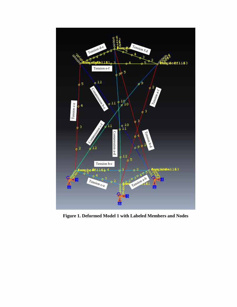
Figure 1. Deformed Model 1 with Labeled Members and Nodes
Tension b-c
Tension e-f
Co
mp
ression
a-d

Table 1. Reaction Forces, Displacements, and Rotations at Nodes Along Length of Members in Model 1
Note: Force reaction results are in pounds and displacements are in inches.
Field Output reported at nodes for part: comp a-d-1 Node Label RT.RT1 RT.RT2 RT.RT3 U.U1 U.U2 U.U3 UR.UR1 UR.UR2 UR.UR3 @Loc 1 @Loc 1 @Loc 1 @Loc 1 @Loc 1 @Loc 1 @Loc 1 @Loc 1 @Loc 1 ----------------------------------------------------------------------------------------------------------------------------------------------------------------- 1 0. 0. 0. 577.521E-06 457.893E-06 322.927E-06 -436.057E-06 539.108E-06 314.048E-06 2 -4.98086 -94.7724 100.000 4.98086E-36 94.7724E-36 -100.000E-36 -60.7516E-36 42.2080E-36 21.4101E-36 3 0. 0. 0. 75.6040E-03 -29.1524E-03 -12.1021E-03 5.98059E-03 2.83366E-03 2.63968E-03 4 0. 0. 0. 83.0888E-03 -40.2668E-03 -18.8081E-03 6.60995E-03 2.72295E-03 2.63969E-03 5 0. 0. 0. 359.911E-06 320.604E-06 214.992E-06 -388.317E-06 420.936E-06 239.476E-06 6 0. 0. 0. 196.374E-06 199.445E-06 124.514E-06 -320.840E-06 307.943E-06 170.779E-06 7 0. 0. 0. 83.8904E-06 101.141E-06 55.7120E-06 -233.628E-06 200.123E-06 107.967E-06 8 0. 0. 0. 19.4389E-06 32.4183E-06 12.8016E-06 -126.682E-06 97.4750E-06 51.0411E-06 9 0. 0. 0. 56.5387E-03 -9.99804E-03 -1.09799E-03 3.30697E-03 3.16689E-03 2.54680E-03 10 0. 0. 0. 37.4391E-03 -116.472E-06 3.59057E-03 1.32850E-03 3.10405E-03 2.26781E-03 11 0. 0. 0. 20.3697E-03 3.14896E-03 4.01957E-03 45.1664E-06 2.64514E-03 1.80269E-03 12 0. 0. 0. 7.39441E-03 2.45487E-03 2.24502E-03 -543.017E-06 1.79016E-03 1.15143E-03 13 0. 0. 0. 81.6035E-03 -37.9776E-03 -17.4204E-03 6.58478E-03 2.72738E-03 2.63969E-03 14 0. 0. 0. 80.1153E-03 -35.7051E-03 -16.0443E-03 6.50925E-03 2.74066E-03 2.63969E-03 15 0. 0. 0. 78.6213E-03 -33.4656E-03 -14.6915E-03 6.38338E-03 2.76280E-03 2.63969E-03 16 0. 0. 0. 77.1185E-03 -31.2759E-03 -13.3736E-03 6.20716E-03 2.79380E-03 2.63969E-03 Field Output reported at nodes for part: comp b-e-1 Node Label RT.RT1 RT.RT2 RT.RT3 U.U1 U.U2 U.U3 UR.UR1 UR.UR2 UR.UR3 @Loc 1 @Loc 1 @Loc 1 @Loc 1 @Loc 1 @Loc 1 @Loc 1 @Loc 1 @Loc 1 ----------------------------------------------------------------------------------------------------------------------------------------------------------------- 1 0. 0. 0. -12.5546E-03 80.0534E-03 -12.1045E-03 -5.44031E-03 3.76560E-03 2.64407E-03 2 0. 0. 0. -6.66679E-03 92.0919E-03 -18.8126E-03 -5.65892E-03 4.36637E-03 2.64407E-03 3 0. 0. 0. -685.163E-06 271.065E-06 323.151E-06 -248.560E-06 -647.146E-06 314.375E-06 4 84.5651 43.0672 99.9905 -84.5651E-36 -43.0671E-36 -99.9905E-36 -6.13804E-36 -73.6857E-36 21.4010E-36 5 0. 0. 0. -11.4719E-03 82.4266E-03 -13.3763E-03 -5.51901E-03 3.98188E-03 2.64407E-03 6 0. 0. 0. -10.3260E-03 84.8228E-03 -14.6947E-03 -5.58022E-03 4.15009E-03 2.64407E-03 7 0. 0. 0. -9.13260E-03 87.2362E-03 -16.0480E-03 -5.62394E-03 4.27025E-03 2.64407E-03 8 0. 0. 0. -7.90760E-03 89.6612E-03 -17.4245E-03 -5.65018E-03 4.34234E-03 2.64407E-03 9 0. 0. 0. -5.82436E-03 5.17695E-03 2.24589E-03 -1.27814E-03 -1.36547E-03 1.15305E-03 10 0. 0. 0. -12.9155E-03 16.0688E-03 4.02138E-03 -2.31210E-03 -1.28335E-03 1.80535E-03 11 0. 0. 0. -18.6239E-03 32.4859E-03 3.59273E-03 -3.35045E-03 -400.802E-06 2.27129E-03 12 0. 0. 0. -19.6151E-03 53.9676E-03 -1.09695E-03 -4.39319E-03 1.28218E-03 2.55086E-03 13 0. 0. 0. -37.7787E-06 606.140E-09 12.8069E-06 -20.9841E-06 -158.401E-06 51.0569E-06 14 0. 0. 0. -129.490E-06 22.0265E-06 55.7401E-06 -56.3322E-06 -302.316E-06 108.023E-06 15 0. 0. 0. -270.829E-06 70.2503E-06 124.585E-06 -106.044E-06 -431.745E-06 170.898E-06 16 0. 0. 0. -457.489E-06 151.267E-06 215.127E-06 -170.121E-06 -546.689E-06 239.681E-0

Table 1 (cont.). Reaction Forces, Displacements, and Rotations at Nodes Along Length of Members in Model 1
Note: Force reaction results are in pounds and displacements are in inches.
Field Output reported at nodes for part: comp c-f-1 Node Label RT.RT1 RT.RT2 RT.RT3 U.U1 U.U2 U.U3 UR.UR1 UR.UR2 UR.UR3 @Loc 1 @Loc 1 @Loc 1 @Loc 1 @Loc 1 @Loc 1 @Loc 1 @Loc 1 @Loc 1 ----------------------------------------------------------------------------------------------------------------------------------------------------------------- 1 0. 0. 0. 107.965E-06 -728.764E-06 323.020E-06 684.566E-06 108.369E-06 314.388E-06 2 -79.5842 51.7052 100.009 79.5842E-36 -51.7052E-36 -100.009E-36 66.8887E-36 31.5463E-36 21.4030E-36 3 0. 0. 0. -63.0400E-03 -50.8954E-03 -12.1013E-03 -540.185E-06 -6.59215E-03 2.64415E-03 4 0. 0. 0. -76.4052E-03 -51.8162E-03 -18.8038E-03 -950.943E-06 -7.08158E-03 2.64415E-03 5 0. 0. 0. 97.8383E-06 -471.754E-06 215.047E-06 558.396E-06 126.081E-06 239.694E-06 6 0. 0. 0. 74.6361E-06 -269.634E-06 124.543E-06 426.854E-06 124.100E-06 170.910E-06 7 0. 0. 0. 45.7006E-06 -123.143E-06 55.7233E-06 289.940E-06 102.426E-06 108.033E-06 8 0. 0. 0. 18.3743E-06 -33.0192E-06 12.8037E-06 147.656E-06 61.0597E-06 51.0627E-06 9 0. 0. 0. -36.9253E-03 -43.9654E-03 -1.09795E-03 1.08630E-03 -4.44455E-03 2.55092E-03 10 0. 0. 0. -18.8205E-03 -32.3666E-03 3.59031E-03 2.02202E-03 -2.70070E-03 2.27133E-03 11 0. 0. 0. -7.45818E-03 -19.2161E-03 4.01934E-03 2.26698E-03 -1.36059E-03 1.80538E-03 12 0. 0. 0. -1.57115E-03 -7.63108E-03 2.24497E-03 1.82115E-03 -424.236E-06 1.15307E-03 13 0. 0. 0. -73.6806E-03 -51.6753E-03 -17.4168E-03 -934.512E-06 -7.06200E-03 2.64415E-03 14 0. 0. 0. -70.9689E-03 -51.5236E-03 -16.0414E-03 -885.221E-06 -7.00327E-03 2.64415E-03 15 0. 0. 0. -68.2830E-03 -51.3502E-03 -14.6893E-03 -803.069E-06 -6.90538E-03 2.64415E-03 16 0. 0. 0. -65.6358E-03 -51.1444E-03 -13.3720E-03 -688.057E-06 -6.76834E-03 2.64415E-03 Field Output reported at nodes for part: ten a-b-1 Node Label RT.RT1 RT.RT2 RT.RT3 U.U1 U.U2 U.U3 UR.UR1 UR.UR2 UR.UR3 @Loc 1 @Loc 1 @Loc 1 @Loc 1 @Loc 1 @Loc 1 @Loc 1 @Loc 1 @Loc 1 ----------------------------------------------------------------------------------------------------------------------------------------------------------------- 1 0. 0. 0. 577.521E-06 457.893E-06 322.927E-06 354.969E-06 614.843E-06 -83.3401E-06 2 0. 0. 0. 324.991E-06 420.523E-06 322.972E-06 354.969E-06 614.843E-06 -83.3380E-06 3 0. 0. 0. 72.4633E-06 383.153E-06 323.017E-06 354.969E-06 614.843E-06 -83.3410E-06 4 0. 0. 0. -180.071E-06 345.785E-06 323.062E-06 354.969E-06 614.843E-06 -83.3388E-06 5 0. 0. 0. -432.601E-06 308.416E-06 323.107E-06 354.969E-06 614.843E-06 -83.3459E-06 6 0. 0. 0. -685.163E-06 271.065E-06 323.151E-06 354.969E-06 614.843E-06 -83.3604E-06 Field Output reported at nodes for part: ten a-f-1 Node Label RT.RT1 RT.RT2 RT.RT3 U.U1 U.U2 U.U3 UR.UR1 UR.UR2 UR.UR3 @Loc 1 @Loc 1 @Loc 1 @Loc 1 @Loc 1 @Loc 1 @Loc 1 @Loc 1 @Loc 1 ----------------------------------------------------------------------------------------------------------------------------------------------------------------- 1 0. 0. 0. -63.0400E-03 -50.8954E-03 -12.1013E-03 -7.73169E-03 -6.90848E-03 45.7061E-03 2 0. 0. 0. -50.3172E-03 -40.6238E-03 -9.61649E-03 -7.73185E-03 -6.90848E-03 45.7061E-03 3 0. 0. 0. -37.5942E-03 -30.3530E-03 -7.13175E-03 -7.73205E-03 -6.90862E-03 45.7061E-03 4 0. 0. 0. -24.8704E-03 -20.0826E-03 -4.64688E-03 -7.73202E-03 -6.90876E-03 45.7060E-03 5 0. 0. 0. -12.1464E-03 -9.81212E-03 -2.16196E-03 -7.73207E-03 -6.90876E-03 45.7060E-03 6 0. 0. 0. 577.521E-06 457.893E-06 322.927E-06 -7.73218E-03 -6.90876E-03 45.7060E-03 Field Output reported at nodes for part: ten b-c-1 Node Label RT.RT1 RT.RT2 RT.RT3 U.U1 U.U2 U.U3 UR.UR1 UR.UR2 UR.UR3 @Loc 1 @Loc 1 @Loc 1 @Loc 1 @Loc 1 @Loc 1 @Loc 1 @Loc 1 @Loc 1 ----------------------------------------------------------------------------------------------------------------------------------------------------------------- 1 0. 0. 0. -685.163E-06 271.065E-06 323.151E-06 -115.515E-21 10.9218E-09 -83.3190E-06 2 0. 0. 0. -526.537E-06 71.0989E-06 323.125E-06 -115.515E-21 10.9218E-09 -83.3190E-06 3 0. 0. 0. -367.912E-06 -128.867E-06 323.099E-06 -115.515E-21 10.9218E-09 -83.3190E-06 4 0. 0. 0. -209.286E-06 -328.832E-06 323.073E-06 -115.515E-21 10.9218E-09 -83.3190E-06 5 0. 0. 0. -50.6609E-06 -528.798E-06 323.047E-06 -115.515E-21 10.9218E-09 -83.3190E-06 6 0. 0. 0. 107.965E-06 -728.764E-06 323.020E-06 -115.515E-21 10.9218E-09 -83.3190E-06
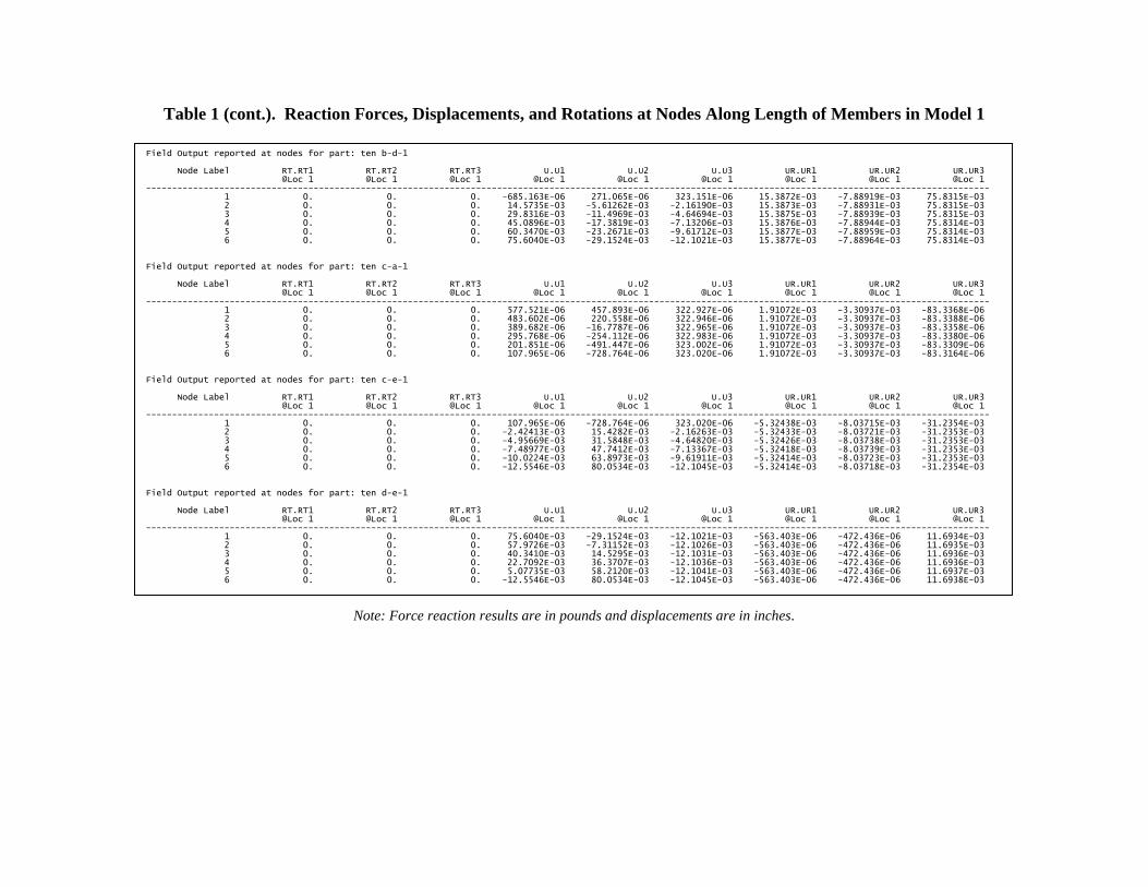
Table 1 (cont.). Reaction Forces, Displacements, and Rotations at Nodes Along Length of Members in Model 1
Note: Force reaction results are in pounds and displacements are in inches.
Field Output reported at nodes for part: ten b-d-1 Node Label RT.RT1 RT.RT2 RT.RT3 U.U1 U.U2 U.U3 UR.UR1 UR.UR2 UR.UR3 @Loc 1 @Loc 1 @Loc 1 @Loc 1 @Loc 1 @Loc 1 @Loc 1 @Loc 1 @Loc 1 ----------------------------------------------------------------------------------------------------------------------------------------------------------------- 1 0. 0. 0. -685.163E-06 271.065E-06 323.151E-06 15.3872E-03 -7.88919E-03 75.8315E-03 2 0. 0. 0. 14.5735E-03 -5.61262E-03 -2.16190E-03 15.3873E-03 -7.88931E-03 75.8315E-03 3 0. 0. 0. 29.8316E-03 -11.4969E-03 -4.64694E-03 15.3875E-03 -7.88939E-03 75.8315E-03 4 0. 0. 0. 45.0896E-03 -17.3819E-03 -7.13206E-03 15.3876E-03 -7.88944E-03 75.8314E-03 5 0. 0. 0. 60.3470E-03 -23.2671E-03 -9.61712E-03 15.3877E-03 -7.88959E-03 75.8314E-03 6 0. 0. 0. 75.6040E-03 -29.1524E-03 -12.1021E-03 15.3877E-03 -7.88964E-03 75.8314E-03 Field Output reported at nodes for part: ten c-a-1 Node Label RT.RT1 RT.RT2 RT.RT3 U.U1 U.U2 U.U3 UR.UR1 UR.UR2 UR.UR3 @Loc 1 @Loc 1 @Loc 1 @Loc 1 @Loc 1 @Loc 1 @Loc 1 @Loc 1 @Loc 1 ----------------------------------------------------------------------------------------------------------------------------------------------------------------- 1 0. 0. 0. 577.521E-06 457.893E-06 322.927E-06 1.91072E-03 -3.30937E-03 -83.3368E-06 2 0. 0. 0. 483.602E-06 220.558E-06 322.946E-06 1.91072E-03 -3.30937E-03 -83.3388E-06 3 0. 0. 0. 389.682E-06 -16.7787E-06 322.965E-06 1.91072E-03 -3.30937E-03 -83.3358E-06 4 0. 0. 0. 295.768E-06 -254.112E-06 322.983E-06 1.91072E-03 -3.30937E-03 -83.3380E-06 5 0. 0. 0. 201.851E-06 -491.447E-06 323.002E-06 1.91072E-03 -3.30937E-03 -83.3309E-06 6 0. 0. 0. 107.965E-06 -728.764E-06 323.020E-06 1.91072E-03 -3.30937E-03 -83.3164E-06 Field Output reported at nodes for part: ten c-e-1 Node Label RT.RT1 RT.RT2 RT.RT3 U.U1 U.U2 U.U3 UR.UR1 UR.UR2 UR.UR3 @Loc 1 @Loc 1 @Loc 1 @Loc 1 @Loc 1 @Loc 1 @Loc 1 @Loc 1 @Loc 1 ----------------------------------------------------------------------------------------------------------------------------------------------------------------- 1 0. 0. 0. 107.965E-06 -728.764E-06 323.020E-06 -5.32438E-03 -8.03715E-03 -31.2354E-03 2 0. 0. 0. -2.42413E-03 15.4282E-03 -2.16263E-03 -5.32433E-03 -8.03721E-03 -31.2353E-03 3 0. 0. 0. -4.95669E-03 31.5848E-03 -4.64820E-03 -5.32426E-03 -8.03738E-03 -31.2353E-03 4 0. 0. 0. -7.48977E-03 47.7412E-03 -7.13367E-03 -5.32418E-03 -8.03739E-03 -31.2353E-03 5 0. 0. 0. -10.0224E-03 63.8973E-03 -9.61911E-03 -5.32414E-03 -8.03723E-03 -31.2353E-03 6 0. 0. 0. -12.5546E-03 80.0534E-03 -12.1045E-03 -5.32414E-03 -8.03718E-03 -31.2354E-03 Field Output reported at nodes for part: ten d-e-1 Node Label RT.RT1 RT.RT2 RT.RT3 U.U1 U.U2 U.U3 UR.UR1 UR.UR2 UR.UR3 @Loc 1 @Loc 1 @Loc 1 @Loc 1 @Loc 1 @Loc 1 @Loc 1 @Loc 1 @Loc 1 ----------------------------------------------------------------------------------------------------------------------------------------------------------------- 1 0. 0. 0. 75.6040E-03 -29.1524E-03 -12.1021E-03 -563.403E-06 -472.436E-06 11.6934E-03 2 0. 0. 0. 57.9726E-03 -7.31152E-03 -12.1026E-03 -563.403E-06 -472.436E-06 11.6935E-03 3 0. 0. 0. 40.3410E-03 14.5295E-03 -12.1031E-03 -563.403E-06 -472.436E-06 11.6936E-03 4 0. 0. 0. 22.7092E-03 36.3707E-03 -12.1036E-03 -563.403E-06 -472.436E-06 11.6936E-03 5 0. 0. 0. 5.07735E-03 58.2120E-03 -12.1041E-03 -563.403E-06 -472.436E-06 11.6937E-03 6 0. 0. 0. -12.5546E-03 80.0534E-03 -12.1045E-03 -563.403E-06 -472.436E-06 11.6938E-03 Field Output reported at nodes for part: ten e-f-1 Node Label RT.RT1 RT.RT2 RT.RT3 U.U1 U.U2 U.U3 UR.UR1 UR.UR2 UR.UR3 @Loc 1 @Loc 1 @Loc 1 @Loc 1 @Loc 1 @Loc 1 @Loc 1 @Loc 1 @Loc 1 ----------------------------------------------------------------------------------------------------------------------------------------------------------------- 1 0. 0. 0. -12.5546E-03 80.0534E-03 -12.1045E-03 2.35900E-03 -858.285E-06 11.6935E-03 2 0. 0. 0. -22.6516E-03 53.8638E-03 -12.1039E-03 2.35900E-03 -858.285E-06 11.6935E-03 3 0. 0. 0. -32.7487E-03 27.6741E-03 -12.1032E-03 2.35900E-03 -858.285E-06 11.6936E-03 4 0. 0. 0. -42.8458E-03 1.48440E-03 -12.1026E-03 2.35900E-03 -858.285E-06 11.6936E-03 5 0. 0. 0. -52.9429E-03 -24.7054E-03 -12.1019E-03 2.35900E-03 -858.285E-06 11.6936E-03 6 0. 0. 0. -63.0400E-03 -50.8954E-03 -12.1013E-03 2.35900E-03 -858.285E-06 11.6937E-03

Table 1 (cont.). Reaction Forces, Displacements, and Rotations at Nodes Along Length of Members in Model 1
Note: Force reaction results are in pounds and displacements are in inches.
Field Output reported at nodes for part: ten e-f-1 Node Label RT.RT1 RT.RT2 RT.RT3 U.U1 U.U2 U.U3 UR.UR1 UR.UR2 UR.UR3 @Loc 1 @Loc 1 @Loc 1 @Loc 1 @Loc 1 @Loc 1 @Loc 1 @Loc 1 @Loc 1 ----------------------------------------------------------------------------------------------------------------------------------------------------------------- 1 0. 0. 0. -12.5546E-03 80.0534E-03 -12.1045E-03 2.35900E-03 -858.285E-06 11.6935E-03 2 0. 0. 0. -22.6516E-03 53.8638E-03 -12.1039E-03 2.35900E-03 -858.285E-06 11.6935E-03 3 0. 0. 0. -32.7487E-03 27.6741E-03 -12.1032E-03 2.35900E-03 -858.285E-06 11.6936E-03 4 0. 0. 0. -42.8458E-03 1.48440E-03 -12.1026E-03 2.35900E-03 -858.285E-06 11.6936E-03 5 0. 0. 0. -52.9429E-03 -24.7054E-03 -12.1019E-03 2.35900E-03 -858.285E-06 11.6936E-03 6 0. 0. 0. -63.0400E-03 -50.8954E-03 -12.1013E-03 2.35900E-03 -858.285E-06 11.6937E-03 Field Output reported at nodes for part: ten f-d-1 Node Label RT.RT1 RT.RT2 RT.RT3 U.U1 U.U2 U.U3 UR.UR1 UR.UR2 UR.UR3 @Loc 1 @Loc 1 @Loc 1 @Loc 1 @Loc 1 @Loc 1 @Loc 1 @Loc 1 @Loc 1 ----------------------------------------------------------------------------------------------------------------------------------------------------------------- 1 0. 0. 0. -63.0400E-03 -50.8954E-03 -12.1013E-03 873.463E-06 -4.95480E-03 11.6936E-03 2 0. 0. 0. -35.3112E-03 -46.5468E-03 -12.1014E-03 873.463E-06 -4.95480E-03 11.6936E-03 3 0. 0. 0. -7.58224E-03 -42.1981E-03 -12.1016E-03 873.463E-06 -4.95480E-03 11.6937E-03 4 0. 0. 0. 20.1467E-03 -37.8495E-03 -12.1018E-03 873.463E-06 -4.95480E-03 11.6936E-03 5 0. 0. 0. 47.8754E-03 -33.5009E-03 -12.1019E-03 873.463E-06 -4.95480E-03 11.6935E-03 6 0. 0. 0. 75.6040E-03 -29.1524E-03 -12.1021E-03 873.463E-06 -4.95480E-03 11.6935E-03
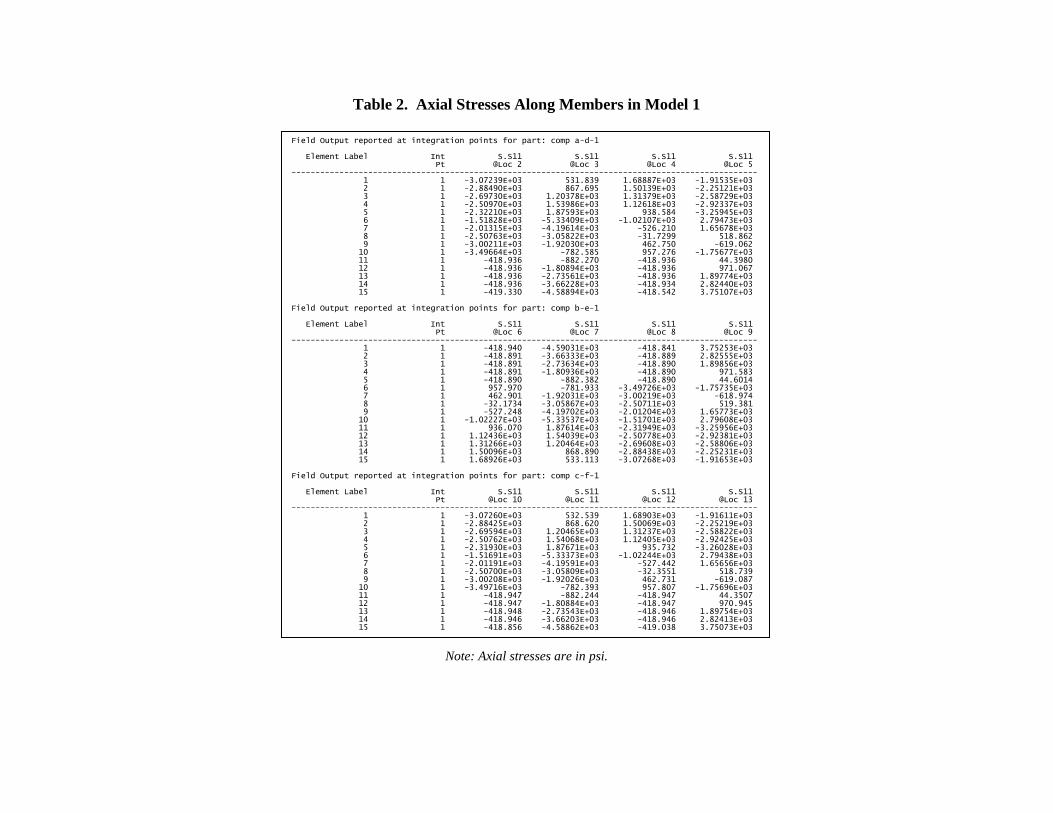
Table 2. Axial Stresses Along Members in Model 1
Note: Axial stresses are in psi.
Field Output reported at integration points for part: comp a-d-1 Element Label Int S.S11 S.S11 S.S11 S.S11 Pt @Loc 2 @Loc 3 @Loc 4 @Loc 5 ------------------------------------------------------------------------------------------------- 1 1 -3.07239E+03 531.839 1.68887E+03 -1.91535E+03 2 1 -2.88490E+03 867.695 1.50139E+03 -2.25121E+03 3 1 -2.69730E+03 1.20378E+03 1.31379E+03 -2.58729E+03 4 1 -2.50970E+03 1.53986E+03 1.12618E+03 -2.92337E+03 5 1 -2.32210E+03 1.87593E+03 938.584 -3.25945E+03 6 1 -1.51828E+03 -5.33409E+03 -1.02107E+03 2.79473E+03 7 1 -2.01315E+03 -4.19614E+03 -526.210 1.65678E+03 8 1 -2.50763E+03 -3.05822E+03 -31.7299 518.862 9 1 -3.00211E+03 -1.92030E+03 462.750 -619.062 10 1 -3.49664E+03 -782.585 957.276 -1.75677E+03 11 1 -418.936 -882.270 -418.936 44.3980 12 1 -418.936 -1.80894E+03 -418.936 971.067 13 1 -418.936 -2.73561E+03 -418.936 1.89774E+03 14 1 -418.936 -3.66228E+03 -418.934 2.82440E+03 15 1 -419.330 -4.58894E+03 -418.542 3.75107E+03 Field Output reported at integration points for part: comp b-e-1 Element Label Int S.S11 S.S11 S.S11 S.S11 Pt @Loc 6 @Loc 7 @Loc 8 @Loc 9 ------------------------------------------------------------------------------------------------- 1 1 -418.940 -4.59031E+03 -418.841 3.75253E+03 2 1 -418.891 -3.66333E+03 -418.889 2.82555E+03 3 1 -418.891 -2.73634E+03 -418.890 1.89856E+03 4 1 -418.891 -1.80936E+03 -418.890 971.583 5 1 -418.890 -882.382 -418.890 44.6014 6 1 957.970 -781.933 -3.49726E+03 -1.75735E+03 7 1 462.901 -1.92031E+03 -3.00219E+03 -618.974 8 1 -32.1734 -3.05867E+03 -2.50711E+03 519.381 9 1 -527.248 -4.19702E+03 -2.01204E+03 1.65773E+03 10 1 -1.02227E+03 -5.33537E+03 -1.51701E+03 2.79608E+03 11 1 936.070 1.87614E+03 -2.31949E+03 -3.25956E+03 12 1 1.12436E+03 1.54039E+03 -2.50778E+03 -2.92381E+03 13 1 1.31266E+03 1.20464E+03 -2.69608E+03 -2.58806E+03 14 1 1.50096E+03 868.890 -2.88438E+03 -2.25231E+03 15 1 1.68926E+03 533.113 -3.07268E+03 -1.91653E+03 Field Output reported at integration points for part: comp c-f-1 Element Label Int S.S11 S.S11 S.S11 S.S11 Pt @Loc 10 @Loc 11 @Loc 12 @Loc 13 ------------------------------------------------------------------------------------------------- 1 1 -3.07260E+03 532.539 1.68903E+03 -1.91611E+03 2 1 -2.88425E+03 868.620 1.50069E+03 -2.25219E+03 3 1 -2.69594E+03 1.20465E+03 1.31237E+03 -2.58822E+03 4 1 -2.50762E+03 1.54068E+03 1.12405E+03 -2.92425E+03 5 1 -2.31930E+03 1.87671E+03 935.732 -3.26028E+03 6 1 -1.51691E+03 -5.33373E+03 -1.02244E+03 2.79438E+03 7 1 -2.01191E+03 -4.19591E+03 -527.442 1.65656E+03 8 1 -2.50700E+03 -3.05809E+03 -32.3551 518.739 9 1 -3.00208E+03 -1.92026E+03 462.731 -619.087 10 1 -3.49716E+03 -782.393 957.807 -1.75696E+03 11 1 -418.947 -882.244 -418.947 44.3507 12 1 -418.947 -1.80884E+03 -418.947 970.945 13 1 -418.948 -2.73543E+03 -418.946 1.89754E+03 14 1 -418.946 -3.66203E+03 -418.946 2.82413E+03 15 1 -418.856 -4.58862E+03 -419.038 3.75073E+03
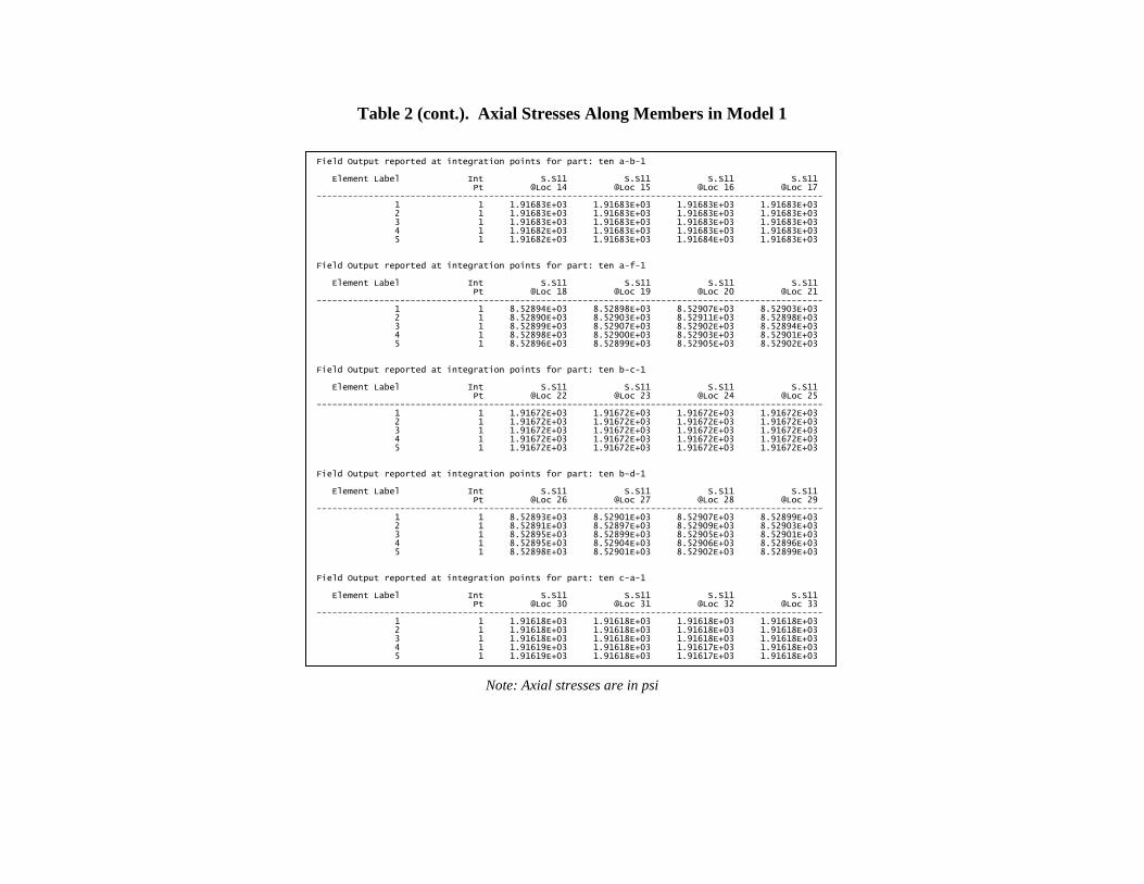
Table 2 (cont.). Axial Stresses Along Members in Model 1
Note: Axial stresses are in psi
Field Output reported at integration points for part: ten a-b-1 Element Label Int S.S11 S.S11 S.S11 S.S11 Pt @Loc 14 @Loc 15 @Loc 16 @Loc 17 ------------------------------------------------------------------------------------------------- 1 1 1.91683E+03 1.91683E+03 1.91683E+03 1.91683E+03 2 1 1.91683E+03 1.91683E+03 1.91683E+03 1.91683E+03 3 1 1.91683E+03 1.91683E+03 1.91683E+03 1.91683E+03 4 1 1.91682E+03 1.91683E+03 1.91683E+03 1.91683E+03 5 1 1.91682E+03 1.91683E+03 1.91684E+03 1.91683E+03 Field Output reported at integration points for part: ten a-f-1 Element Label Int S.S11 S.S11 S.S11 S.S11 Pt @Loc 18 @Loc 19 @Loc 20 @Loc 21 ------------------------------------------------------------------------------------------------- 1 1 8.52894E+03 8.52898E+03 8.52907E+03 8.52903E+03 2 1 8.52890E+03 8.52903E+03 8.52911E+03 8.52898E+03 3 1 8.52899E+03 8.52907E+03 8.52902E+03 8.52894E+03 4 1 8.52898E+03 8.52900E+03 8.52903E+03 8.52901E+03 5 1 8.52896E+03 8.52899E+03 8.52905E+03 8.52902E+03 Field Output reported at integration points for part: ten b-c-1 Element Label Int S.S11 S.S11 S.S11 S.S11 Pt @Loc 22 @Loc 23 @Loc 24 @Loc 25 ------------------------------------------------------------------------------------------------- 1 1 1.91672E+03 1.91672E+03 1.91672E+03 1.91672E+03 2 1 1.91672E+03 1.91672E+03 1.91672E+03 1.91672E+03 3 1 1.91672E+03 1.91672E+03 1.91672E+03 1.91672E+03 4 1 1.91672E+03 1.91672E+03 1.91672E+03 1.91672E+03 5 1 1.91672E+03 1.91672E+03 1.91672E+03 1.91672E+03 Field Output reported at integration points for part: ten b-d-1 Element Label Int S.S11 S.S11 S.S11 S.S11 Pt @Loc 26 @Loc 27 @Loc 28 @Loc 29 ------------------------------------------------------------------------------------------------- 1 1 8.52893E+03 8.52901E+03 8.52907E+03 8.52899E+03 2 1 8.52891E+03 8.52897E+03 8.52909E+03 8.52903E+03 3 1 8.52895E+03 8.52899E+03 8.52905E+03 8.52901E+03 4 1 8.52895E+03 8.52904E+03 8.52906E+03 8.52896E+03 5 1 8.52898E+03 8.52901E+03 8.52902E+03 8.52899E+03 Field Output reported at integration points for part: ten c-a-1 Element Label Int S.S11 S.S11 S.S11 S.S11 Pt @Loc 30 @Loc 31 @Loc 32 @Loc 33 ------------------------------------------------------------------------------------------------- 1 1 1.91618E+03 1.91618E+03 1.91618E+03 1.91618E+03 2 1 1.91618E+03 1.91618E+03 1.91618E+03 1.91618E+03 3 1 1.91618E+03 1.91618E+03 1.91618E+03 1.91618E+03 4 1 1.91619E+03 1.91618E+03 1.91617E+03 1.91618E+03 5 1 1.91619E+03 1.91618E+03 1.91617E+03 1.91618E+03
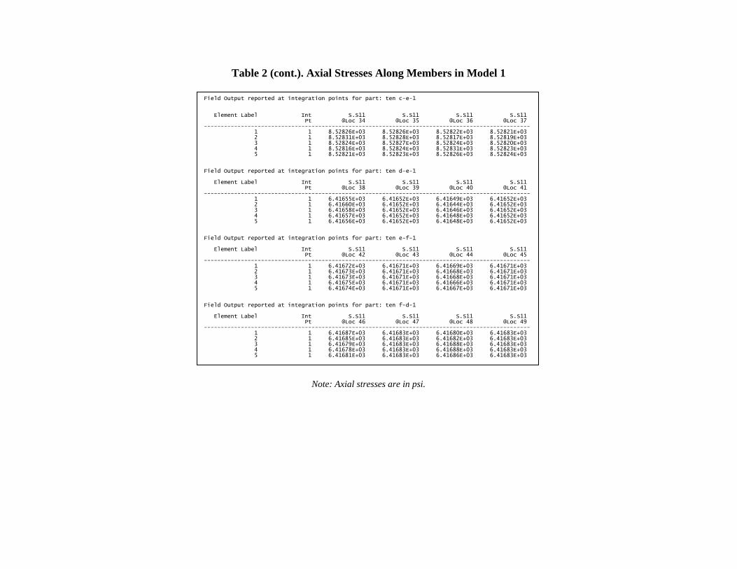
Table 2 (cont.). Axial Stresses Along Members in Model 1
Note: Axial stresses are in psi.
Field Output reported at integration points for part: ten c-e-1
Element Label Int S.S11 S.S11 S.S11 S.S11 Pt @Loc 34 @Loc 35 @Loc 36 @Loc 37 ------------------------------------------------------------------------------------------------- 1 1 8.52826E+03 8.52826E+03 8.52822E+03 8.52821E+03 2 1 8.52831E+03 8.52828E+03 8.52817E+03 8.52819E+03 3 1 8.52824E+03 8.52827E+03 8.52824E+03 8.52820E+03 4 1 8.52816E+03 8.52824E+03 8.52831E+03 8.52823E+03 5 1 8.52821E+03 8.52823E+03 8.52826E+03 8.52824E+03 Field Output reported at integration points for part: ten d-e-1 Element Label Int S.S11 S.S11 S.S11 S.S11 Pt @Loc 38 @Loc 39 @Loc 40 @Loc 41 ------------------------------------------------------------------------------------------------- 1 1 6.41655E+03 6.41652E+03 6.41649E+03 6.41652E+03 2 1 6.41660E+03 6.41652E+03 6.41644E+03 6.41652E+03 3 1 6.41658E+03 6.41652E+03 6.41646E+03 6.41652E+03 4 1 6.41657E+03 6.41652E+03 6.41648E+03 6.41652E+03 5 1 6.41656E+03 6.41652E+03 6.41648E+03 6.41652E+03 Field Output reported at integration points for part: ten e-f-1 Element Label Int S.S11 S.S11 S.S11 S.S11 Pt @Loc 42 @Loc 43 @Loc 44 @Loc 45 ------------------------------------------------------------------------------------------------- 1 1 6.41672E+03 6.41671E+03 6.41669E+03 6.41671E+03 2 1 6.41673E+03 6.41671E+03 6.41668E+03 6.41671E+03 3 1 6.41673E+03 6.41671E+03 6.41668E+03 6.41671E+03 4 1 6.41675E+03 6.41671E+03 6.41666E+03 6.41671E+03 5 1 6.41674E+03 6.41671E+03 6.41667E+03 6.41671E+03 Field Output reported at integration points for part: ten f-d-1 Element Label Int S.S11 S.S11 S.S11 S.S11 Pt @Loc 46 @Loc 47 @Loc 48 @Loc 49 ------------------------------------------------------------------------------------------------- 1 1 6.41687E+03 6.41683E+03 6.41680E+03 6.41683E+03 2 1 6.41685E+03 6.41683E+03 6.41682E+03 6.41683E+03 3 1 6.41679E+03 6.41683E+03 6.41688E+03 6.41683E+03 4 1 6.41678E+03 6.41683E+03 6.41688E+03 6.41683E+03 5 1 6.41681E+03 6.41683E+03 6.41686E+03 6.41683E+03