
Analysis of seismic activity on the western part of the ... Árni Guðnason.pdfFigure 2.3 An example...
81
Analysis of seismic activity on the western part of the Reykjanes Peninsula, SW Iceland, December 2008 – May 2009 Egill Árni Guðnason Faculty of Earth Sciences University of Iceland 2014
-
Upload
truongmien -
Category
Documents
-
view
221 -
download
3
Transcript of Analysis of seismic activity on the western part of the ... Árni Guðnason.pdfFigure 2.3 An example...

Analysis of seismic activity on the western part of the Reykjanes Peninsula, SW Iceland, December 2008 – May 2009
Egill Árni Guðnason
Faculty of Earth Sciences University of Iceland
2014


Analysis of seismic activity on the western part of the Reykjanes Peninsula, SW Iceland, December 2008 – May 2009
Egill Árni Guðnason
60 ECTS thesis submitted in partial fulfillment of a Magister Scientiarum degree in Geophysics
Advisors Kristján Ágústsson Ólafur G. Flóvenz
Faculty Representative Bryndís Brandsdóttir
Faculty of Earth Sciences School of Engineering and Natural Sciences
University of Iceland Reykjavik, April 2014

Analysis of seismic activity on the western part of the Reykjanes Peninsula, SW Iceland, December 2008 – May 2009 Seismicity on the Reykjanes Peninsula 60 ECTS thesis submitted in partial fulfillment of a Magister Scientiarum degree in Geophysics Copyright © 2014 Egill Árni Guðnason All rights reserved Faculty of Earth Sciences School of Engineering and Natural Sciences University of Iceland Askja, Sturlugata 7 101 Reykjavik Iceland Telephone: 525 4000 Bibliographic information: Egill Árni Guðnason, 2014, Analysis of seismic activity on the western part of the Reykjanes Peninsula, SW Iceland, December 2008 – May 2009, Master’s thesis, Faculty of Earth Sciences, University of Iceland, pp. 83. Printing: Háskólaprent Reykjavik, Iceland, April 2014

iii
Abstract In the autumn of 2008 the energy company HS Orka hf. had planned an injection test in the Reykjanes geothermal field in Iceland. This provided an opportunity to study eventual induced seismicity. The Icelandic regional seismic network was not considered sensitive enough to detect and locate small size seismic events. To increase the seismic sensitivity in the area, five temporary seismic stations were installed by the Institute of Earth Sciences at the University of Iceland in December 2008. In addition, data from six SIL stations and three seismic stations operated by the University of Wisconsin were available for the same period. The area under study encompassed mainly the western part of the Reykjanes Peninsula, i.e. the area west of longitude -22.4°, with the addition of the Fagradalsfjall area to the east. The seismic stations of the University of Iceland had to be dismantled in the middle of May 2009, before full-scale injection started. Some small-scale injection was carried out in the Reykjanes geothermal field during the recording period, while more extensive injection was carried out in the Svartsengi geothermal field. Seismic activity from December 2008 to May 2009 was less than on average in the study area. Induced seismicity was not observed in the Reykjanes geothermal field but indications of induced seismicity were observed in the Svartsengi geothermal field. In the Fagradalsfjall area, earthquake activity was mainly confined to one significant earthquake swarm, during the study period, located beneath the southwestern slopes of Fagradalsfjall.
Útdráttur Haustið 2008 ákvað HS Orka að hefja niðurdælingaprófanir á jarðhitasvæðinu á Reykjanesi. Því gafst tækifæri til að rannsaka mögulega örvaða smáskjálftavirkni. Til þess að fylgjast með henni setti Jarðvísindastofnun Háskóla Íslands upp fimm skjálftamæla á Reykjanesskaga í desember sama ár, sem voru reknir fram í maí árið 2009. Að auki voru fáanleg gögn frá sex skjálftamælum Veðurstofu Íslands af Reykjanesskaga, í SIL mælakerfinu, ásamt gögnum frá þremur mælum frá Háskólanum í Wisconsin fyrir sama tímabil. Skjálftamælanetið samanstóð því af fjórtán skjálftamælum og var mælanetið þéttast á plötuskilunum frá Reykjanesi að Svartsengi. Skjálftamælar Jarðvísindastofnunar voru teknir upp áður en niðurdæling hófst fyrir alvöru. Lítilsháttar niðurdæling var þó á þessu tímabili á Reykjanesi, en mun meiri í Svartsengi. Jarðskjálftavirkni á Reykjanesskaga u.þ.b. vestur af Grindavíkurvegi (-22.4° vestur) á tímabilinu var minni en hún hefur verið að meðaltali á rekstrartíma SIL kerfisins síðustu 17 ár. SIL kerfi Veðurstofunnar eitt og sér staðsetti 20 jarðskjálfta á tímabilinu, samanborið við 122 jarðskjálfta staðsetta sameiginlega af skjálftamælaneti Jarðvísindastofnunar, sex SIL-mælum og þremur mælum Háskólans í Wisconsin. Örfáir jarðskjálftar voru á Reykjanesi. Meirihluti jarðskjálftanna var í Svartsengi í grennd við niðurdælingaholurnar SV-17 og SV-24. Engar vísbendingar fundust um smáskjálfta af völdum niðurdælingar á Reykjanesi en í Svartsengi bendir staðsetning meirihluta jarðskjálftanna til þess að um örvaða skjálftavirkni af völdum niðurdælingar geti verið að ræða. Hrina smáskjálfta var á tímabilinu undir suðvesturhlíðum Fagradalsfjalls, um 7 km norðaustur af Grindavík.


v
Table of Contents List of Figures ..................................................................................................................... vi List of Tables ....................................................................................................................... ix Acknowledgements .............................................................................................................. x 1 Introduction ..................................................................................................................... 1
1.1 Tectonic, geological and geothermal setting ........................................................... 3 1.2 The seismic network ................................................................................................ 5 1.3 Data and processing ................................................................................................. 7 1.4 Historic seismicity on the Reykjanes Peninsula ...................................................... 9
1.4.1 The SIL seismic network ............................................................................. 10
2 Methods .......................................................................................................................... 13 2.1 Non-Linear Location ............................................................................................. 13 2.2 Double-difference earthquake location ................................................................. 14 2.3 Focal mechanism solutions ................................................................................... 17
3 Analysis of the seismic activity .................................................................................... 21 3.1 Explosions in the Helguvík area ............................................................................ 23 3.2 Results for the Reykjanes geothermal field ........................................................... 24
3.2.1 Seismicity compared with injection and production in Reykjanes .............. 25 3.2.2 Focal mechanism solutions in Reykjanes .................................................... 26
3.3 Results for the Svartsengi geothermal field .......................................................... 27 3.3.1 Seismicity compared with injection and production in Svartsengi .............. 28 3.3.2 An earthquake swarm in Svartsengi ............................................................ 29 3.3.3 Relative relocations of an earthquake swarm in Svartsengi ........................ 31 3.3.4 Focal mechanism solutions in Svartsengi .................................................... 32
3.4 Results for the Fagradalsfjall area ......................................................................... 33 3.4.1 An earthquake swarm in the Fagradalsfjall area .......................................... 34 3.4.2 Relative relocations of an earthquake swarm in the Fagradalsfjall area ...... 36 3.4.3 Focal mechanism solutions in the Fagradalsfjall area ................................. 39
4 Conclusions .................................................................................................................... 41 References .......................................................................................................................... 45 Appendix 1: List of earthquakes in Reykjanes ............................................................... 51 Appendix 2: List of earthquakes in Svartsengi ............................................................... 53 Appendix 3: List of earthquakes in the Fagradalsfjall area .......................................... 57 Appendix 4: Focal mechanism solutions in Reykjanes .................................................. 61 Appendix 5: Focal mechanism solutions in Svartsengi .................................................. 63 Appendix 6: Focal mechanism solutions in the Fagradalsfjall area ............................. 67

vi
List of Figures Figure 1.1 The plate boundary in Iceland (Hjaltadóttir, 2009). Fissure swarms are
shaded with grey colour and central volcanoes outlined with thin, black lines (from Einarsson and Sæmundsson, 1987). Transform zones and offshore ridge segments are drawn as broken, black lines. Abbreviations refer to main text. ............................................................................................... 1
Figure 1.2 A geological map of the Reykjanes Peninsula, showing the fissure swarms and high temperature areas along with the Reykjanes Ridge on the inset (based on a geological map of Iceland by Jóhannesson and Sæmundsson, 1999, modified from Harðardóttir et al., 2009). ................................................ 3
Figure 1.3 The seismic stations on the Reykjanes peninsula. Black triangles show the location of the permanent SIL stations, yellow the stations of the University of Wisconsin and blue the temporary seismic monitoring network of the University of Iceland. ................................................................. 6
Figure 1.4 One-dimensional velocity models used for NonLinLoc locations. ...................... 8
Figure 2.1 The double-difference earthquake location algorithm (Waldhauser and Ellsworth, 2000). Solid and open (initial locations) circles represent trial hypocenters linked to neighboring events by cross-correlation (solid lines) or catalog data (dashed lines). The corresponding slowness vectors, s, for two events, i and j, w/ respect to two stations, k and l, are shown. Thick arrows (Δx) indicate the relocation vector obtained from equation (5), and dt is the travel time difference between events i and j, observed at station k and l, respectively. .......................................................... 16
Figure 2.2 A schematic diagram of a focal mechanism, showing the stereographic projection on a horizontal plane of the lower half of the focal sphere surrounding the earthquake source (A), and the ambiguity in choosing which of the two nodal planes is the fault plane (B) (http://earthquake.usgs.gov/learn/topics/images/beachball.gif). ..................... 18
Figure 2.3 An example of a focal mechanism solution, as plotted by FPFIT, for an event located in an earthquake swarm in Svartsengi on the 6th of March 2009. The large circle is a lower-hemisphere projection of the adopted focal mechanism solution and first-motion data. Dilatational rays are represented by circle symbols, compressional rays by plus symbols, upgoing rays are indicated by bold-face symbols and downgoing rays by light-lined symbols. The letters P and T are centered on the points corresponding to the P- and T-axes, respectively. The small circle shows the distribution of possible range of orientations of P- and T-axes consistent with the data, allowing for uncertainty. .......................................... 19
Figure 3.1 Location of earthquakes (red dots) and explosions (blue dots) on the Reykjanes Peninsula, based on the temporary network and six SIL seismic stations. ................................................................................................ 21

vii
Figure 3.2 Comparison of depths of earthquakes west of longitude -22.4°, located only with available SIL stations, versus earthquakes located with the temporary network together with the SIL stations. The data points of the depth comparison are shown with red crosses, while the green line represents the modelled regression line. .......................................................... 22
Figure 3.3 Cumulative depth distribution of earthquakes west of longitude -22.4°, showing the fraction of earthquakes located at corresponding depth and shallower. ......................................................................................................... 23
Figure 3.4 Five seconds plots of vertical component traces for i) an explosion in Helguvík at station NYL on the 7th of April (top) and ii) an earthquake in Svartsengi at station HAFN on the 6th of March (bottom). Both waveforms are bandpass-filtered between 4-40 Hz. ......................................... 24
Figure 3.5 Earthquakes in Reykjanes from December 2008 to May 2009. E-W and N-S depth sections are shown, as well as the boreholes in the Reykjanes well-field with small yellow crosses. Yellow color indicates slightly altered ground, pink indicates heavily altered ground and dark grey indicates recent volcanic material. ................................................................... 25
Figure 3.6 Production and injection (top) in the Reykjanes geothermal field and temporal distribution of earthquakes (bottom) during the recording period. ............................................................................................................... 26
Figure 3.7 Focal mechanism solutions for earthquakes in Reykjanes. ............................... 27
Figure 3.8 Earthquakes in Svartsengi from December 2008 to May 2009. E-W and N-S depth sections are shown, as well as the boreholes in the Svartsengi well-field with small yellow crosses. Yellow color indicates slightly altered ground. ................................................................................................. 28
Figure 3.9 Production and injection (top) in the Svartsengi geothermal field and temporal distribution of earthquakes (bottom) during the recording period. ............................................................................................................... 29
Figure 3.10 The earthquake swarm of the 6th of March, 2009, and the origin time of individual earthquakes. The blue and red lines on the E-W and N-S depth sections show the direction and extent of the injection boreholes, SV-17 and SV-24, respectively. Yellow color indicates slightly altered ground. ........ 30
Figure 3.11 Relative relocations of the earthquake swarm from the 6th of March, 2009, and the origin time of individual earthquakes. The blue and red lines on the E-W and N-S depth sections show the direction and extent of the injection boreholes, SV-17 and SV-24, respectively. Yellow color indicates slightly altered ground. ..................................................................... 31
Figure 3.12 Focal mechanism solutions for earthquakes in Svartsengi. ............................. 32
Figure 3.13 Earthquakes in the Fagradalsfjall area from December 2008 to May 2009, with E-W and N-S depth sections. .......................................................... 34
viii
Figure 3.14 Selected earthquakes of the earthquake swarm in Fagradalsfjall in February 2009, with E-W and N-S depth sections and the origin time of individual earthquakes. .................................................................................... 35
Figure 3.15 Five seconds plots of vertical component traces for seven events of the earthquake swarm in the Fagradalsfjall area, observed at station NYL. All waveforms are bandpass-filtered between 4-40 Hz. ................................... 37
Figure 3.16 Relative relocations of the selected earthquakes of the earthquake swarm in Fagradalsfjall in February 2009, with E-W and N-S depth sections and the origin time of individual earthquakes. ................................................. 38
Figure 3.17 Focal mechanism solutions for earthquakes in the Fagradalsfjall area. ........ 39

ix
List of Tables Table 1 Seismic stations, location, elevation and seismometers on the Reykjanes
Peninsula. ........................................................................................................... 7
Table 2 List of earthquakes in Reykjanes. ........................................................................... 51
Table 3 List of earthquakes in Svartsengi. .......................................................................... 53
Table 4 List of earthquakes in the Fagradalsfjall area. ...................................................... 57

x
Acknowledgements This thesis is submitted to the University of Iceland in partial fulfillment of a degree of Master of Science in Geophysics. The research was supervised by Kristján Ágústsson and Ólafur G. Flóvenz at Iceland GeoSurvey (ÍSOR), and Bryndís Brandsdóttir at the University of Iceland. First and foremost, I would like to thank my supervisors for their guidance and encouragement throughout my work, but especially my main supervisor, Kristján, for all the support, patience and time spent explaining and discussing various seismological as well as technical problems that arose during my work.
This project was funded by the Geothermal Research Group (GEORG) in Iceland, the power company HS Orka hf., and the 7th Framework Programme of the EU through the GEISER project. HS Orka hf., the Icelandic Meteorological Office, Bryndís Brandsdóttir at the University of Iceland, Ólafur Guðmundsson at the University of Uppsala and Reykjavik University and Kurt Feigl at the University of Wisconsin kindly allowed use of the seismic data. Vatnaskil Consulting Engineers supplied the production and injection data for Reykjanes and Svartsengi. The majority of figures in this thesis were created using the GMT-software (Wessel and Smith, 1998) and ObsPy, the Python Toolbox for seismology, was used to plot focal mechanisms and corresponding maps, as well as waveform traces.
I would like to thank Iceland GeoSurvey for hiring me for this work. Many thanks go to my co-workers, especially Gunnlaugur M. Einarsson for GMT assistance and my cousin Ingvar Þór Magnússon for helping with various programming problems. Last but not least, I wish to thank my girlfriend Fríða, my family and all my friends, who never gave up encouraging me to finish this work.

1
1 Introduction Iceland is an island in the North Atlantic Ocean, shaped by volcanism and glaciations. It is the onshore continuation of the Mid-Atlantic Ridge, i.e. from the Reykjanes Ridge (RR) in the southwest to the Kolbeinsey Ridge (KR) in the north. Because of the interplay between the Mid-Atlantic Ridge and the Iceland Mantle Plume, the plate boundary in Iceland consists of a series of volcanic and seismic zones (Figure 1.1).
The plate boundary from the Reykjanes Peninsula (RP) in the west, up through the Hengill triple junction, and extending to the Langjökull ice cap, has been termed the Reykjanes-Langjökull Volcanic Zone (Sigmundsson, 2006). The Reykjanes-Langjökull Volcanic Zone can be divided into two zones, the Reykjanes Peninsula oblique rift, southwest of the Hengill volcanic area, and the less oblique Western Volcanic Zone (WVZ), north of the Hengill volcanic area (Einarsson, 1991, 2008). The plate boundary from the south coast of Iceland, extending north to the Vatnajökull ice cap, is termed the Eastern Volcanic Zone (EVZ). Similarly, the plate boundary north of the Vatnajökull ice cap and extending to the north coast of Iceland is termed the Northern Volcanic Zone (NVZ).
Figure 1.1 The plate boundary in Iceland (Hjaltadóttir, 2009). Fissure swarms are shaded with grey colour and central volcanoes outlined with thin, black lines (from Einarsson and Sæmundsson, 1987). Transform zones and offshore ridge segments are drawn as broken, black lines. Abbreviations refer to main text.
The third arm of the Hengill triple junction is the transform zone in South Iceland, the South Iceland Seismic Zone (SISZ), which connects the Reykjanes Peninsula to the Eastern Volcanic Zone (EVZ). Another transform zone, the Tjörnes Fracture Zone (TFZ),

2
connects the Northern Volcanic Zone to the offshore Kolbeinsey Ridge. The two transform zones are the main seismic zones of the plate boundary in Iceland, although seismic activity occurs everywhere on the plate boundary.
The discrimination between natural and induced earthquakes can be a difficult task. In general, induced seismicity is defined as earthquake activity resulting from human activity, i.e. earthquake activity that is expected to be higher than the normal level of historical seismicity. Seismicity can be induced in numerous ways. For example, by fluid injection or extraction at a rate that causes failure along fault planes, by thermal or chemical changes caused by fluid injection, or by hydrofracturing.
Over the past two years, some of Europe’s main geothermal research institutions have been working on a research project in the field of induced seismicity, i.e. the GEISER (Geothermal Engineering Integrating of Induced Seismicity in Reservoirs) project, partly funded by the European Commission. The project was coordinated by GFZ Potsdam in Germany, and involved 12 additional partners. Iceland GeoSurvey was a large participant in the project on behalf of Iceland, and Iceland GeoSurvey’s part in the project was funded by the Geothermal Research Group in Iceland (GEORG). The aim of the project was to, among other things, understand the nature of induced seismicity, propose licensing and monitoring guidelines for local authorities, and to investigate strategies for stimulation of geothermal reservoirs without producing earthquakes that could be felt or cause damage.
One of the specific topics of the project was analysis of induced seismicity from representative geothermal reservoirs throughout Europe. At Iceland GeoSurvey, data from four geothermal fields in Iceland, Reykjanes, Svartsengi, Hengill and Krafla, were investigated as a part of the project.
In the autumn of 2008 the energy company HS Orka hf. had planned an injection test in the Reykjanes geothermal field in Iceland. The regional seismic network in Iceland (SIL) was not considered sensitive enough to detect and locate eventual small size induced seismic events. To increase the seismic sensitivity of the SIL network in the area during the test, five temporary seismic stations were installed in December 2008, by the Institute of Earth Sciences at the University of Iceland (UI). In addition, data from three seismic stations operated by the University of Wisconsin were available for the same period.
Reykjanes is the SW tip of the Reykjanes Peninsula, precisely where the axis of the oceanic Reykjanes Ridge comes on shore in Iceland (Figure 1.2). The Reykjanes geothermal field is in the centre of Reykjanes and has been utilized for electrical power production by HS Orka hf. since 2006 with a power production of 100 MWe at present. About 13 km to the ENE of Reykjanes is the Svartsengi geothermal field. Svartsengi, similar to Reykjanes, is located on the plate boundaries of the Reykjanes Peninsula. It has been utilized by HS Orka hf. since 1976 to provide hot water for domestic heating (150 MWth) and production of electricity (75 MWe).
Exploitation of geothermal fluids in Reykjanes and Svartsengi has caused both pressure drawdown and a cumulative surface subsidence within the wellfields since the start of production (Eysteinsson, 1999). To reduce this drawdown, injection of wastefluids is currently carried out in both areas.

3
The injection test at Reykjanes was delayed, and the UI seismic stations had to be dismantled in the middle of May 2009, before full-scale injection started. However, small-scale injection was carried out in the Reykjanes geothermal field during the recording period, while more extensive injection was carried out in the Svartsengi geothermal field as a part of the reservoir management.
During the recording period from December 2008 to May 2009, seismic activity was less than on average in the study area. Induced seismicity was not observed in the Reykjanes geothermal field but indications of induced seismicity were observed in the Svartsengi geothermal field. The temporary network of seismic stations, together with data from six SIL stations, was successfully installed in order to detect smaller and consequently a larger number of earthquakes compared to the routine locations of the SIL network alone.
This thesis focuses on seismic data analysis on the Reykjanes Peninsula from December 2008 to May 2009, as well as comparison between the seismic activity and the injection and production data in Reykjanes and Svartsengi. The area under study encompasses mainly the western part of the Reykjanes Peninsula with a main focus on the plate boundaries from Reykjanes to Svartsengi, i.e. the area west of longitude -22.4° with the addition of the Fagradalsfjall area just east of the main study area.
1.1 Tectonic, geological and geothermal setting
Figure 1.2 A geological map of the Reykjanes Peninsula, showing the fissure swarms and high temperature areas along with the Reykjanes Ridge on the inset (based on a geological map of Iceland by Jóhannesson and Sæmundsson, 1999, modified from Harðardóttir et al., 2009).
The plate boundary in Iceland consists of volcanic rifts and fault zones, because of the interplay between the Mid-Atlantic Ridge (i.e. the Reykjanes Ridge) and the Iceland Mantle Plume. The westward motion of the spreading ridge with respect to the mantle plume has resulted in a number of eastward rift jumps and an increasing offset of the plate

4
boundary in Iceland from the Mid-Atlantic Ridge (Einarsson, 1991). As a result, most of the plate boundary in Iceland is oriented at an oblique angle to the spreading direction.
The Mid-Atlantic Ridge comes onshore at the southwestern tip of Iceland, on the Reykjanes Peninsula (Figure 1.1, 1.2). The peninsula marks the southwesternmost part of the active volcanic and rift zones of Iceland, and forms the transition from the Reykjanes Ridge in the west to the South Iceland Seismic Zone in the east, southeast of the Hengill high-temperature area (Einarsson, 1991). The peninsula is probably best described as an oblique spreading rift, defining the boundaries of the American and Eurasian plates, striking N80°E compared to the spreading direction of N102.1±1.1°E (Tryggvason, 1968; Klein et al., 1973; DeMets et al., 1994).
The Reykjanes Peninsula is one of the most seismically active parts of Iceland, especially at the microearthquake level. The seismic zone, which extends from the western tip of the peninsula towards the Hengill triple junction in the east, is not a single fault, but rather a series of strike-slip and normal faults (Einarsson and Björnsson, 1979). Seismicity is continuous along the plate boundary, and earthquake surveys have shown that seismicity on the western part of the peninsula, as in Reykjanes and Svartsengi, and of the Reykjanes Ridge to the southwest, is generally characterized by episodic earthquake swarms, whereas fewer but larger earthquakes are typical of the eastern part (Tryggvason, 1973; Einarsson, 1991).
The geology of the Reykjanes Peninsula is characterized by Pleistocene basaltic lavas, hyaloclastite ridges and postglacial lava flows (Sæmundsson and Einarsson, 1980). Postglacial lavas from shield volcanoes and eruptive fissures are dominant for the western part of the peninsula, which is our area of study. Rifting on the peninsula began after a rift jump 6-7 Ma ago (Sæmundsson, 1978), and the most recent eruption occurred in the 13th century (Thordarson and Larsen, 2007). Eruptive activity on the peninsula appears to repeat itself approximately every thousand years, with an eruptive period of a few hundred years and a non-eruptive period of several hundred years (Sigurgeirsson, 1995). The eruptions have occurred on a series of NE-SW trending eruptive fissures which can be grouped into four en echelon volcanic fissure swarms (Sæmundsson, 1978). The fissure swarms consist of normal faults and extensional tension fractures in addition to the eruptive fissures, and they are intersected at an oblique angle by a series of near vertical N-S right-lateral strike-slip faults (Keiding et al., 2009).
Five high-temperature geothermal fields are present on the Reykjanes Peninsula (Figure 1.2). They are located on the obliquely rifting plate boundaries of the American and Eurasian plates, primarily at the intersection of the eruptive fissures and the strike-slip faults. The geothermal fields are, from west to east, the Reykjanes, Eldvörp, Svartsengi, Krýsuvík and Brennisteinsfjöll fields. Two of the seven installed geothermal power plants in Iceland are located in Reykjanes and Svartsengi, producing about 30% (175 MWe in total) of all electricity production from geothermal energy in Iceland.
Inevitably, the extraction and exploitation of geothermal fluids can have several side effects. Pressure drawdown and contraction of the rock matrix are two effects causing subsidence above the reservoir. The local deformation is often so large that it obscures the deformation due to tectonic processes such as plate boundary deformation. These effects may well lead to decreased well field productivity or inflow of colder fluids into the

5
reservoir. In order to prevent pressure drawdown and subsidence, geothermal fluid is nowadays typically injected back into the geothermal reservoirs after utilization.
Subsidence and pressure drawdown have been documented by levelling and gravity measurements in Reykjanes and Svartsengi throughout the years. Subsidence in Svartsengi was first documented by repeated levelling and gravity measurements in 1975-1999 (Eysteinsson, 1999). Results showed subsidence rates between 7-14 mm/year with the highest rates during the first years of production, and a linear connection between the rate of subsidence and pressure drawdown observed at 900 meter depth in boreholes. The average rate of subsidence has however decreased since full-time injection started in Svartsengi in 2001, to around 6 mm/year in 1999-2004 and 2 mm/year in 2004-2008 (Magnússon, 2009). The shape of the subsidence in Svartsengi is elliptical, and elongated in the NE-SW direction, thus aligning with the trend of the normal faults and volcanic fractures in the area. In 2008-2010, the subsidence in Svartsengi stopped, i.e. the average subsidence rate decreased to almost 0 mm/year.
In Reykjanes, results showed no sign of subsidence before the start of production in May 2006, but then subsidence abruptly started, and average subsidence rates of around 14-16 mm/year in 2004-2008 were measured, with the highest rates during the first years of production, and then around 14 mm/year in 2008-2010 after the start of continuous injection (Magnússon, 2009). The elliptical shape of subsidence in Reykjanes is similar to Svartsengi, with a clear NE-SW direction, thus aligning with the trend of the volcanic fractures in the area.
In order to avert this process and to support the natural recharge into the system, an injection of geothermal water has been carried out in Svartsengi and Reykjanes, since 2001 and 2008 respectively.
1.2 The seismic network The seismic network consisted of three subnets (Figure 1.3 and Table 1). The stations ATLA, ELDV, HAFN, LINU and SAND were temporary stations operated by the University of Iceland. They were composed of REFTEK-130 data loggers and Lennartz LE-3D/5s seismometers. The stations ARNAR, CWSS and FFPS were also temporary stations installed by Kurt Feigl at the University of Wisconsin. The stations were composed of Guralp data loggers and seismometers, i.e. a CMG-DM24 data logger and a CMG-3T seismometer. Finally, the eight stations GRV, NYL, RNE, VOG, KAS, KRI, SAN and VOS are permanent stations that are part of the regional seismic network in Iceland, the SIL network, operated and maintained by the Icelandic Meteorological Office (IMO). At this time, seven of the SIL stations used the CRD3 digitizer, but one of them (RNE station) used the Guralp CMG-DM24 data logger. Seven of the SIL stations used the Lennartz LE-3D/5s seismometer, but one of them (KRI station) used the Lennartz LE-3D/1s seismometer. The sampling rate was 100 samples per second at all stations.

6
Figure 1.3 The seismic stations on the Reykjanes peninsula. Black triangles show the location of the permanent SIL stations, yellow the stations of the University of Wisconsin and blue the temporary seismic monitoring network of the University of Iceland.
The area covered by the twelve westernmost seismic stations was a region about 16 km times 17 km, with an average distance of 6.6 km between stations and a main focus on the plate boundaries from Reykjanes to Svartsengi.

7
Table 1 Seismic stations, location, elevation and seismometers on the Reykjanes Peninsula.
Station name Latitude [°N] Longitude [°W] Elevation [m] Seismometer
ATLA 63.82214 -22.61711 14 LE-3D/5s ELDV 63.85887 -22.53194 59 LE-3D/5s HAFN 63.92868 -22.63860 19 LE-3D/5s LINU 63.87368 -22.58812 54 LE-3D/5s SAND 63.86705 -22.70217 19 LE-3D/5s GRV 63.85716 -22.45583 52 LE-3D/5s NYL 63.97368 -22.73792 7 LE-3D/5s RNE 63.81681 -22.70563 19 LE-3D/5s VOG 63.96967 -22.39285 7 LE-3D/5s KAS 64.02290 -21.85200 108 LE-3D/5s KRI 63.87810 -22.07646 146 LE-3D/1s SAN 64.05601 -21.57013 208 LE-3D/5s VOS 63.85279 -21.70357 8 LE-3D/5s ARNAR 63.90313 -22.45915 23 CMG-3T CWSS 63.83633 -22.65467 8 CMG-3T FFPS 63.82800 -22.55218 25 CMG-3T
1.3 Data and processing Seismic data from the different subnets were on different formats. They were converted to Mini-SEED format, and then processed and earthquakes located using the SeisComp seismological software for data acquisition and processing (www.seiscomp3.org). The SeisComp software offers offline automatic event detection and location. Automatically located events were manually examined to improve time picks and to read first-motion polarities of the seismic waves. Furthermore, the records were manually scanned to see if any events escaped the automatic event detection.
In the location process, the NonLinLoc (Non-Linear Location) locator algorithm (Lomax et al., 2000) was used, that has been implemented into the SeisComp software. The NonLinLoc program performs earthquake locations in 3D models using non-linear search techniques. Our 3D model grid uses a 1 km grid node spacing along the x, y and z axes.
Local magnitudes (ML) were calculated using the SeisComp software. To model the relationship between local magnitudes of the SIL network and local magnitudes calculated by SeisComp, a least-squares linear regression was performed for earthquakes recorded by both the SIL network and the seismic network of this study, using Gnuplot. The modelled relationship is represented by a function y = f(x), where x is the independent variable (i.e. SeisComp magnitudes) and y the dependent variable (i.e. SIL magnitudes). The optimum values of the parameters of the function f(x) (f(x) = -0.76 + 0.90·x) were then used to correct the local magnitudes calculated by SeisComp, to make them consistent with the local magnitudes of the SIL network.

8
Crustal velocities affect seismic wave propagation and travel times. Therefore, a good knowledge of crustal structures is necessary for accurate earthquake locations. In this study, the SIL linear-gradient velocity model was used. The SIL model is an average model derived from the western part of the South Iceland Seismic Tomography (SIST) refraction profile (Bjarnason et al., 1993). A linear-gradient velocity model derived from the Reykjanes-Iceland Seismic Experiment (RISE) refraction profile (Weir et al., 2001) was also used for comparison, but gave less constrained results for the majority of events, i.e. higher RMS residuals and larger location uncertainties in latitude, longitude and depth, compared to the SIL model (Figure 1.4).
Figure 1.4 One-dimensional velocity models used for NonLinLoc locations.
Records from the five stations operated by the University of Iceland were continuous and data quality was for the most part good. Records from the three stations of the University of Wisconsin had many gaps and a very low signal-to-noise ratio. It turned out that they were more or less useless for this purpose. Records from six of the eight permanent SIL stations were continuous during the recording period, and data quality was good. However, records from stations KRI and VOS were discontinuous or empty during the recording period and unfortunately useless.
Focal mechanism solutions were generated using the program FPFIT of Reasenberg and Oppenheimer (1985), which calculates best fit double-couple focal mechanism solutions from the polarity data. The focal mechanism solutions were limited to events with strike, dip and rake uncertainties less than 20°.

9
The earthquakes in earthquake swarms in Svartsengi and Fagradalsfjall were relatively relocated using HypoDD, a program to compute hypocentre locations using a double-difference algorithm (Waldhauser, 2001).
Vatnaskil Consulting Engineers provided production and injection data for the Reykjanes and Svartsengi geothermal fields. Production data (in kg/s) for the Reykjanes geothermal field are given at one hour intervals for each production hole, and at six hour intervals for each production hole in the Svartsengi geothermal field, resulting in a fairly good temporal resolution of the production data. The injection volumes for both fields are only available as average values per month, resulting in a poor temporal resolution of the injection data.
1.4 Historic seismicity on the Reykjanes Peninsula
Seismic activity on the Reykjanes Peninsula is variable in time and with different characteristics along the peninsula. On the western part of the peninsula and the Reykjanes Ridge to the southwest, earthquake swarms are prominent and mainshock-aftershock sequences are rare (Einarsson, 1991; Keiding et al., 2009). Towards east, the mainshock-aftershock character of the activity increases gradually, while the central part of the peninsula acts as a transition between the two.
Historical descriptions exist and they are quite reliable since the construction of a lighthouse on Reykjanes in 1878 and permanent settlement in the area thereafter (Halldórsson, 2011). The first installation of a seismometer in Iceland was in 1909 (Einarsson and Björnsson, 1987). It was removed in 1914 (Tryggvason, 1973) but reinstalled in 1925 and seismicity in Iceland has been continuously recorded since then.
Annals report that a quite large event occurred on the Reykjanes Peninsula on the 10th of June 1933 (Halldórsson, 2011). The best known location of the earthquake is close to Fagradalsfjall, at 63.9°N and -22.2°W, and its estimated magnitude was around M 5.5 (Tryggvason, 1973). Earthquake activity on the westernmost part of the Reykjanes Peninsula increased during 1967 to 1970 and stayed high in 1971 to 1975, during which several dense swarms occurred along the plate boundary between 21.9° W and 22.7° W (Einarsson, 1991).
During the summers of 1967 and 1968, microearthquake activity was monitored for the first time on the Reykjanes Peninsula when portable, one-component, analog seismographs were operated for a few days near the Reykjanes and Krýsuvík geothermal areas (Ward and Björnsson, 1971). Close to 20 events were located per day in the immediate surroundings of Reykjanes, but no earthquakes were located near Svartsengi. One major swarm occurred in September 1967, on the western part of the Reykjanes Peninsula, with a maximum magnitude event of 4.9 and 14 events larger than magnitude 4 (Tryggvason, 1970). The swarm lasted about 3 days and a significant increase in surface geothermal activity was observed, including revival of geysers (Jónsson, 1968).
In 1971 to 1972, a dense temporary network of up to 23 short-period seismic stations was installed on the western part of the Reykjanes Peninsula, and provided accurate earthquake locations for the first time on the peninsula (Klein et al., 1973, 1977). An intense swarm of several thousand microearthquakes occurred on the peninsula in 1972, approximately one

10
km NNW of the Reykjanes geothermal area, on a less than 2 km wide and 12 km long zone trending NE-SW, interpreted as the currently active American – Eurasian plate boundary. There was no single dominating earthquake in the sequence, and the six largest earthquakes were in the magnitude range of 4.1-4.4. Hypocentral depths were mostly between 2 and 5 km and focal mechanism solutions ranged from normal faulting in the Reykjanes part of the plate-boundary segment to strike-slip faulting to the east of it. No clear relationship was found between the intense earthquake swarm and the geothermal activity of the Reykjanes geothermal area. A few microearthquakes were detected near Svartsengi, but the seismic activity was substantially lower than in Reykjanes.
During May to August in 1993, an array of 15 digital, portable seismographs was operated around the Svartsengi geothermal field in order to monitor microearthquake activity prior to and during an injection test in borehole H-6 inside the production field in Svartsengi (Brandsdóttir et al., 2002). The average rate of injection was 15 l/s, reaching a maximum of 30 l/s. No detectable earthquakes occurred within the Svartsengi geothermal field during the injection period, and it was concluded that the injection pressure was far below the level needed to induce seismicity.
1.4.1 The SIL seismic network
The regional seismic network in Iceland, the SIL (South Iceland lowland) network, has been operated by the Icelandic Meteorological Office and automatically collecting real-time data since June 1991 (Böðvarsson et. al., 1999; Jakobsdóttir et al., 2002). Data since 1995 are available on the internet (http://hraun.vedur.is/ja/viku/).
Since 1995 and until the end of 2012, or during 17 years of operation, the SIL network has located about 1200 events on the Reykjanes Peninsula, west of longitude -22.4° (roughly west of the road to Grindavík). This equals to about 70 events per year on the average. The largest events have reached local magnitudes of 3.6 ML. From a b-value plot (using the Gutenberg-Richter law: log (N) = a - b·M, where N is the number of earthquakes of magnitude M or larger, and a and b are constants) the sensitivity of the network is estimated to be about 1.2 ML for this period, i.e. all earthquakes of magnitude 1.2 ML or larger are recorded, with a b-value close to 1. The seismic stations GRV, VOG and NYL were in full operation since 1997 (Ágústsson et al., 1998). The Reykjanes station (RNE) was installed in May 2008, and it increased the sensitivity of the network in the Reykjanes, Eldvörp and Svartsengi geothermal areas.
Following the start of production in the Reykjanes field in 2006, the SIL network located three short-lived (1-2 days) earthquake swarms offshore, southeast of Reykjanes, trending NE-SW along the periphery of the observed subsidence bowl. Each of the swarms had around 30-60 located events and maximum magnitude events of 2.3, 2.5 and 2.6 ML, respectively. A swarm of around 40 located events also occurred in the same area early 2008 with a maximum magnitude event of 2.5 ML and 6 events larger than magnitude 2 ML.
In October 2013, an intense earthquake swarm occurred mainly offshore at Reykjanes, southeast of the Reykjanes geothermal field, at a distance of about 3 km (Guðnason and Ágústsson, 2014). During 11 days of seismic activity, 880 earthquakes were located by a seismic network operated by Iceland GeoSurvey for HS Orka hf. around the Reykjanes geothermal field, with the addition of four seismic stations of the SIL network. A

11
maximum magnitude event of 4.7 ML occurred on the 13th of October and 25 events had magnitudes of ML ≥ 2.5. Hypocentral depths were mostly between 3 and 5 km and focal mechanism solutions for 13 chosen earthquakes located throughout the active area showed mainly right-lateral strike-slip motion. No clear increase in surface geothermal activity was observed in the Reykjanes geothermal area. A small number of earthquakes have been located by the SIL network in Reykjanes apart from these swarms in 2006, 2008 and 2013.
A small number of earthquakes have been located on the SIL network in Svartsengi since the start of production in the Svartsengi geothermal field in 1976. In 1995-2012, the SIL network only located at an average 10-20 events per year in and around the geothermal area, except for short lived swarms southeast of Svartsengi during two days in July 2007 with a total of 12 located events and a maximum magnitude event of 2.7 ML, and three days in January 2008 with a total of 47 located events, a maximum magnitude event of 3.6 ML and 9 events in the magnitude range of 2-3.6 ML.
The low seismic activity located in Reykjanes and Svartsengi since the start of production, has been postulated to be the result of the fact that the subsidence and pressure drawdown may have increased the friction on potential fault planes, inhibiting fault slip, and thus reduced the microearthquake activity temporarily (Brandsdóttir et al., 2002; Keiding et al., 2010). The swarms located in both areas all seem to occur outside the boundary of the comparable elliptical shapes of subsidence measured in Reykjanes and Svartsengi.

13
2 Methods Seismology is the study of the elastic waves which propagate from a hypocenter, i.e. the source point of an earthquake, through the Earth (Aki and Richards, 1980). The location uncertainty of a determined hypocenter is generally many times larger than the source dimension of the earthquake itself (Waldhauser and Ellsworth, 2000). The accuracy of absolute hypocenter locations relies upon several factors, including the seismic network geometry and density of seismic stations, the number of available phases, arrival-time reading accuracy, and knowledge of the crustal structure.
Using the double-difference earthquake location algorithm on events with similar waveforms, it is possible to reduce the error of relative first arrival-time readings, as well as effectively minimize the effect of errors in structure (Waldhauser and Ellsworth, 2000). Simultaneous relocation of a number of earthquakes can hence increase the location accuracy, and possibly reveal fault patterns.
Earthquake information recorded by seismometers may be transferred to the focal sphere, as a surface on which to describe the radiation pattern of earthquakes (Aki and Richards, 1980). The focal sphere is a convenient device for displaying radiation patterns, and is used to obtain the orientation and direction of slip of the fault plane on which the earthquake occurred.
2.1 Non-Linear Location The NonLinLoc (Non-Linear Location) earthquake location package (Lomax et al., 2000), that has been implemented into the Seiscomp software, is a set of programs for velocity model construction, travel-time calculation and probabilistic, non-linear, earthquake location in 3D structures.
The non-linear location algorithm (Lomax, et al., 2000) uses an inversion approach (by Tarantola and Valette (1982)), and earthquake location methods by Tarantola and Valette (1982), Moser, van Eck and Nolet (1992) and Wittlinger et al. (1993). Observation errors (i.e. phase time picks) and errors in the forward problem (i.e. the travel-time calculation) are assumed to be Gaussian. Given the observed arrival times and the calculated travel times between observing stations and a point in x, y and z space, this assumption of Gaussian observation and forward problem errors allows a direct, analytic calculation of a maximum likelihood origin time. Consequently, the 4D problem of a hypocenter location reduces to a 3D search over x, y and z space.
Given a certain velocity model description, a 3D model grid file is created containing velocity or slowness values. The travel-times between each station and all nodes of the x, y and z spatial grid are calculated once using a 3D version (Le Meur, Virieux and Podvin, 1997) of the Eikonal finite-difference scheme of Podvin and Lecomte (1991) and then stored on disk as travel-time grid files. The forward calculation during location reduces to retrieving the travel-times from the grid files and forming a misfit function. A constant Vp/Vs ratio of 1.78 was specified, and then only P travel-time grids were required for each

14
station. The NonLinLoc program uses the gradients of travel time at the node to estimate the take-off angles at each node, once the travel times are calculated throughout the grid.
The x, y and z volume used for grid-search must be fully contained within the 3D travel-time grids. Therefore, the largest station distance that can be used for location is limited, since the 3D travel-time computation and the size of the output time-grid files grow rapidly with grid dimension.
The NonLinLoc program thus performs earthquake locations in 3D models using non-linear search techniques. The program uses a "flat earth", i.e. a left-handed, rectangular, x, y and z coordinate system with distance units in kilometers. Our 3D model grid uses a 1 km grid node spacing along the x, y and z axes.
2.2 Double-difference earthquake location Earthquakes occurring in an earthquake swarm often produce similar seismic waveforms at a common station, especially if their source mechanisms are identical (i.e. if they originate on the same fault). In general, relative earthquake location techniques take advantage of the fact, that if the hypocentral distance between two earthquakes is small compared to the event-station distance and the velocity heterogeneity, then the seismic ray paths of the two earthquakes, from the source region to a common station, are similar almost along the entire ray paths (Waldhauser and Ellsworth, 2000). The small difference in travel times for the two events recorded at one station will be primarily due to the relatively short distance between the two source locations. Using waveform cross-correlation techniques, the accuracy of relative arrival-time readings can be improved and as a result the absolute locations of earthquakes are improved.
Waldhauser and Ellsworth (2000) developed an efficient earthquake relocation method used in this study. The double-difference algorithm of Waldhauser and Ellsworth allows the simultaneous relocation of a large number of earthquakes occurring over large distances. The location method integrates ordinary catalog travel time measurements and/or P- and S- wave differential travel times, derived from waveform cross-correlation. Residual differences (double-differences) between observed and theoretical travel times are minimized for pairs of earthquakes at each station by iteratively adjusting the vector difference between the hypocentral pairs, while linking all observed event-station pairs together. Compared to ordinary catalog locations, uncertainties in double-difference locations are improved by more than an order of magnitude using the double-difference algorithm.
For an earthquake, i, the arrival time, T, to a seismic station, k, is expressed as a path integral along the seismic ray path as (Waldhauser and Ellsworth, 2000):
, (1)
where τ is the origin time of event i, u is the slowness field and ds is an element of path length. Generally, a truncated Taylor series expansion is used to linearize the otherwise nonlinear equation (1). As a result, the travel time residuals, r, for an event i are linearly related to perturbations, ∆ , to the four current hypocentral parameters for each observation k:

15
∆ , (2)
where , and are the observed and theoretical travel time, respectively, and∆ ∆ , ∆ , ∆ , .
Because cross-correlation methods measure travel time differences between events,
, equation (2) can not be used directly. The relative hypocentral parameters between two events i and j are obtained by taking the difference between equation (2) for a pair of events:
∆ , (3)
where ∆ ∆ , ∆ , ∆ , ∆ is the change in the relative hypocentral parameters between the two events, and the partial derivatives of t with respect to m are the components of the slowness vector of the ray connecting the source and receiver measured at the source (Aki and Richards, 1980). A constant slowness vector is assumed in equation (3) for the two events. The residual between observed and calculated differential travel time between the two events, , is defined as:
. (4)
Equation (4) is defined as the double-difference, and may either use phases with measured arrival times where the observables are absolute travel times, t, or cross-correlation relative travel time differences.
The constant slowness vector assumption is only valid for events that are close together. Therefore, for events farther apart (see Figure 2.1), a valid equation for the change in hypocentral distance between two events, i and j, is obtained by taking the difference between equation (2) and using the appropriate origin time term and slowness vector for each event:
∆ ∆ , (5)
or written out in full:
∆ ∆ ∆ ∆ ∆ ∆ ∆ ∆ . (6)

16
Figure 2.1 The double-difference earthquake location algorithm (Waldhauser and Ellsworth, 2000). Solid and open (initial locations) circles represent trial hypocenters linked to neighboring events by cross-correlation (solid lines) or catalog data (dashed lines). The corresponding slowness vectors, s, for two events, i and j, w/ respect to two stations, k and l, are shown. Thick arrows (Δx) indicate the relocation vector obtained from equation (5), and dt is the travel time difference between events i and j, observed at station k and l, respectively.
The partial derivatives of the travel times, t, for events i and j, with respect to their locations (x, y, z) and origin times (τ), respectively, are calculated for the current hypocenters and the location of the station where the kth phase was recorded (Waldhauser and Ellsworth, 2000). ∆ , ∆ , ∆ and ∆ are the changes required in the hypocentral parameters to make the model better fit the data.
To form a system of linear equations, we combine equation (6) from all hypocentral pairs for a station:
, (7)
where G defines a matrix of size M x 4N (M, number of double-difference observations; N, number of events) containing the partial derivatives, m is a vector of length 4N, ∆ , ∆ , ∆ , ∆ , containing the changes in hypocentral parameters we wish to determine,
d is the data vector containing the double-differences in equation (4), and W is a diagonal matrix to weight each equation. During relocation, we may constrain the mean shift of all earthquakes to zero by extending equation (7) by four equations so that:
∑ ∆ 0, (8)
for each coordinate direction and origin time, respectively. During inversion, equation (8) is usually downweighted to allow the earthquake cluster centroid to move, and to correct for possible errors in the initial absolute locations.

17
2.3 Focal mechanism solutions Focal mechanism solutions are used to describe the radiation pattern of the first P-wave arrivals of an earthquake, on convenient spherical surfaces called focal spheres (Aki and Richards, 1980). The focal sphere is used to obtain the orientation and direction of slip of the fault plane on which the earthquake occurred.
The fault orientation is usually specified by strike and dip, and then rake is used to specify the direction of the slip along the fault plane. For a shear dislocation, the radiation pattern for P-waves is characterized by a quadrantal distribution. The longitudinal first particle motion of a P-wave displacement at a given receiver is either toward or away from the source. On seismograms, the first P-wave arrival either goes up or down, where up signals a compressional arrival and down signals a dilatational arrival.
To obtain a focal mechanism solution from P-wave first motions, particular positions on the focal sphere have to be marked, using a different symbol for compressional and dilatational arrivals. Then, the focal sphere is partitioned by two perpendicular great circles, with each quadrant containing either all compressional or all dilatational arrivals. For P-waves there are two orthogonal nodal planes, and one of them is the fault plane. Due to the double-couple source mechanism (only shear motions on the fault plane), there is an ambiguity in choosing which of the two nodal planes is the fault plane. This ambiguity can sometimes be resolved by comparing the two fault plane orientations to the alignment of small earthquakes and aftershocks. Depending on the quality and distribution of the first P-wave arrivals, more than one focal mechanism solution may fit the data equally well.
A pressure axis (P), which approximates the maximum compressive stress direction, is located in the center of the dilatational quadrant of the focal sphere. A tension axis (T), which approximates the minimum compressive stress direction, is located in the center of the compressional quadrant. These axes are orthogonal to each other, oriented at 45° from the nodal planes, and are the principal axes of the moment tensor.
The focal mechanism solutions are typically displayed on maps as a “beach ball” symbol (http://earthquake.usgs.gov/learn/topics/beachball.php), which is the stereographic projection on a horizontal plane of the lower half of the imaginary, spherical shell (the focal sphere) surrounding the earthquake source. Figure 2.2 shows a schematic diagram of focal mechanisms and illustrates the ambiguity in identifying the fault plane. Figure 2.3 shows an example of a focal mechanism solution for an event located in Svartsengi on the 6th of March 2009.

18
Figure 2.2 A schematic diagram of a focal mechanism, showing the stereographic projection on a horizontal plane of the lower half of the focal sphere surrounding the earthquake source (A), and the ambiguity in choosing which of the two nodal planes is the fault plane (B) (http://earthquake.usgs.gov/learn/topics/images/beachball.gif).

19
Figure 2.3 An example of a focal mechanism solution, as plotted by FPFIT, for an event located in an earthquake swarm in Svartsengi on the 6th of March 2009. The large circle is a lower-hemisphere projection of the adopted focal mechanism solution and first-motion data. Dilatational rays are represented by circle symbols, compressional rays by plus symbols, upgoing rays are indicated by bold-face symbols and downgoing rays by light-lined symbols. The letters P and T are centered on the points corresponding to the P- and T-axes, respectively. The small circle shows the distribution of possible range of orientations of P- and T-axes consistent with the data, allowing for uncertainty.


21
3 Analysis of the seismic activity A total of 340 earthquakes and 40 explosions were located on the Reykjanes Peninsula and in its vicinity from December 2008 to May 2009 (Figure 3.1). In the area covered by the twelve westernmost seismic stations west of longitude -22.4°, or roughly west of the road to Grindavík and Svartsengi, 122 earthquakes were located. During this period, 20 events were located on the SIL network alone in the same area, or around 15% of the located earthquakes.
Figure 3.1 Location of earthquakes (red dots) and explosions (blue dots) on the Reykjanes Peninsula, based on the temporary network and six SIL seismic stations.
Earthquakes were located in various places on the Reykjanes Peninsula, as for example in the Reykjanes and Svartsengi geothermal areas, the Fagradalsfjall area, in Krýsuvík and offshore at Reykjanes (Figure 3.1).
Earthquakes located by the SIL network alone, west of longitude -22.4°, have considerably deeper hypocentres than earthquakes located in this study, with the temporary network together with the SIL stations, although the same velocity model is used for earthquake locations in both cases (Figure 3.3). The difference can to some extent be explained by the different acquisition periods. The SIL data is since 1995, and the majority of the data are from a timespan before the installation and operation of the RNE station in Reykjanes in May 2008. Prior to the operation of the RNE station, the depth resolution in the area was evidently much less. However, there is nothing that indicates that earthquake depths have

22
been different during this recording period (i.e. December 2008 – May 2009), although it cannot be ruled out.
To manually check the depth difference of earthquakes located by the SIL network west of longitude -22.4°, compared with earthquakes located by the temporary network together with the SIL stations, 20 earthquakes of magnitude 0.8 ML or larger, observed on at least 3 of the 4 SIL stations west of longitude -22.4° (i.e. RNE, GRV, VOG and NYL) during this recording period, were chosen for further analysis. For comparison, the earthquakes were first located with the available stations of the temporary network together with the SIL stations, and then only with the available SIL stations. On average, the earthquakes located 1.12 km shallower when only located with the available SIL stations than with the available stations of the temporary network together with the SIL stations. Average location uncertainties in depth were 510 m for earthquakes located with the available stations of the temporary network together with the SIL stations and 1430 m for earthquakes only located with the available SIL stations. Therefore, the different earthquake depths can mainly be explained by the fact that a denser seismic network gives a much better depth determination. The results of this comparison can be seen in Figure 3.2, with the modelled relationship fitted with a least-squares linear regression line, represented by the function y = f(x), and the optimum values of the parameters of the function f(x) = -0.67 + 0.87·x.
Figure 3.2 Comparison of depths of earthquakes west of longitude -22.4°, located only with available SIL stations, versus earthquakes located with the temporary network together with the SIL stations. The data points of the depth comparison are shown with red crosses, while the green line represents the modelled regression line.

23
A cumulative depth distribution of earthquakes most often shows a definite change between a fraction ratio of 0.9 and 1, of earthquakes located at corresponding depth and shallower, as is evident on Figure 3.3 for earthquakes located west of longitude -22.4°. The brittle-ductile boundary has been defined as the depth above which 95% of the seismic activity occurs, i.e. the 95% fraction level (Ágústsson and Flóvenz, 2005, Tryggvason et al., 2002). In this case it is estimated at 5.5 km depth for the temporary network and the SIL stations, and at 9.5 km depth for the SIL network alone (data since 1995). Corresponding brittle-ductile boundary figures based on the 90% fraction level as some authors do (Friðleifsson et al., 2003) are at 4.5 km and 8.5 km depth, respectively.
Figure 3.3 Cumulative depth distribution of earthquakes west of longitude -22.4°, showing the fraction of earthquakes located at corresponding depth and shallower.
3.1 Explosions in the Helguvík area On the 14th of March 2008, Norðurál Century Aluminum started constructions for an aluminum plant near Helguvík, around 10 km northeast of station NYL. From December 2008 to May 2009, 40 explosions were located in the Helguvík area (Figure 3.1). Normally, shallow explosions have a different seismic signature than natural earthquakes. In general, the seismic signal of the Helguvík explosions, containing both the P- and the S-wave, contains lower frequencies than the natural earthquakes on the Reykjanes Peninsula. The P-wave onset is stronger, i.e. contains more energy, than the S-wave onset, different from natural earthquakes where the S-wave onset is usually stronger. This seismic signature was evident for the 40 explosions located in the Helguvík area, and is shown on Figure 3.4 with a comparison of an explosion in the Helguvík area, and an earthquake in Svartsengi of similar magnitude (ca. 0.5 ML) and at a similar distance from the corresponding seismic station (ca. 10 km).

24
Figure 3.4 Five seconds plots of vertical component traces for i) an explosion in Helguvík at station NYL on the 7th of April (top) and ii) an earthquake in Svartsengi at station HAFN on the 6th of March (bottom). Both waveforms are bandpass-filtered between 4-40 Hz.
3.2 Results for the Reykjanes geothermal field The Reykjanes geothermal system is a young and currently heating geothermal system, opposite to the nearest geothermal systems in Eldvörp and Svartsengi (Franzson, 2000). The surface is characterized by Holocene lava flows, NE-trending eruptive fissures, faults and fractures (Sæmundsson, 1978). The uppermost 1 km is characterized by subaquatic / subglacial hyaloclastite formations in between shallow marine sediments. The lithology below the uppermost 1 km is characterized by pillow basalts and intrusive rocks (Franzson et al., 2002).
The geothermal fluid at Reykjanes is a modified sea-water. Temperature logs from boreholes indicate that below the clay cap rock at 500 m depth, the geothermal system follows the boiling point curve, down to about 900 m depth (Friðleifsson et al., 2011). The relatively dense sedimentary succession at 400-1000 m depth forms a kind of cap rock on the deep underlying reservoir. Some steam though manages to rise up through fractures, but at around 900-1100 m depth, a dry steam cap has developed in the center of the geothermal field due to pressure reduction caused by the geothermal fluid production. Below this dry steam cap, the Reykjanes system is liquid dominated with temperatures rising from 270-290 °C up to 320 °C in a freely convecting hydrothermal system, down to at least 2.5 km depth.
Seismicity in and around the Reykjanes geothermal field is shown in Figure 3.5. Earthquake activity from December 2008 to May 2009 was low, with only a few earthquakes located within the production field. The earthquakes that were located within the production field were neither close to the production boreholes nor the injection borehole, RN-20, which is southeast of the production field. A few earthquakes occurred

25
Figure 3.5 Earthquakes in Reykjanes from December 2008 to May 2009. E-W and N-Sdepth sections are shown, as well as the boreholes in the Reykjanes well-field with smallyellow crosses. Yellow color indicates slightly altered ground, pink indicates heavilyaltered ground and dark grey indicates recent volcanic material.
southeast and northwest of the tip of the peninsula, and a few north of the geothermal field. The majority of the 23 earthquakes located in the area (see Appendix 1) occurred between 2 and 5 km depth.
Only 3 of the 23 earthquakes located and shown in Figure 3.5, or 13%, were located by the SIL network alone. Average location uncertainties in latitude, longitude and depth were 420 m, 360 m and 650 m, respectively. The magnitudes of the earthquakes in Reykjanes range from -0.7 to 2.1 ML with the majority of the earthquakes ranging from 0 to 1 ML (see Appendix 1).
3.2.1 Seismicity compared with injection and production in Reykjanes
Production in the Reykjanes field from December 2008 through May 2009 was fairly constant, at 610-660 kg/s, with the exception of a drop in production to 370 kg/s in late April and again to 260 kg/s in early May. For the rest of May, production was stable at around 580 kg/s (Figure 3.6). Injection during the recording period appears to have been rather stable at 150-190 kg/s. However, injection volumes are only available as average values per month. No earthquake swarms occurred during that period in Reykjanes. Due to

26
this and the lack of temporal resolution of the injection rate, no spatial or temporal correlation between the observed scattered seismicity and the injection can be confirmed (Figure 3.6). Furthermore, there is no obvious coupling between the seismic activity and the production in the area.
Figure 3.6 Production and injection (top) in the Reykjanes geothermal field and temporal distribution of earthquakes (bottom) during the recording period.
3.2.2 Focal mechanism solutions in Reykjanes
Focal mechanism solutions were generated for 21 of the 23 earthquakes located in the area, and 12 solutions satisfied the criteria discussed in chapter 1.3 for strike, dip and rake. The focal mechanism solutions can be seen in Figure 3.7, and further examined in Appendix 4. The focal mechanism solutions in Figure 3.7 represent a particular earthquake and compressional quadrants are shown in red. All located earthquakes are shown in orange.
The poor azimuthal coverage of the seismic network relative to the earthquake locations in Reykjanes is not ideal for a detailed study of focal mechanisms. However, the data are sufficient to indicate the type and orientation of faulting of those 12 earthquakes.

27
Figure 3.7 Focal mechanism solutions for earthquakes in Reykjanes.
About half of the focal mechanism solutions for Reykjanes show a significant strike-slip component. The rest of the focal mechanism solutions show mainly reverse faulting with a few focal mechanism solutions showing normal faulting. No clear pattern of focal mechanism solutions is evident.
3.3 Results for the Svartsengi geothermal field The Svartsengi reservoir was initially liquid dominated with a brine reservoir fluid of salinity corresponding to around 2/3 that of sea water (Björnsson and Steingrímsson, 1992). The subsurface geology consists of fresh basaltic lavas at the surface, followed by irregular sections of hyaloclastite and then interglacial and postglacial lava sequences. At depths below 800 m, highly permeable intrusives become dominant.
The geothermal reservoir is divided into three different aquifer systems (Björnsson and Steingrímsson, 1992). The uppermost one is a warm groundwater system at 30-300 m depth with temperatures around 30-100 °C, and a thin freshwater lens on top of saline groundwater. At 300-600 m depth, a steam dominated aquifer, consisting of hyaloclastites with low permeability, separates the uppermost aquifer from the main reservoir. The main reservoir is a liquid dominated brine water system with temperatures of 230-240 °C, at depths greater than 600 m. A two-phase system extends to the surface in the NE part of the wellfield.
Seismicity in and around the Svartsengi geothermal field is shown in Figure 3.8. Earthquake activity during the recording period was noticeably greater than in the nearby geothermal field in Reykjanes, with a few earthquakes located close to the production

28
Figure 3.8 Earthquakes in Svartsengi from December 2008 to May 2009. E-W and N-Sdepth sections are shown, as well as the boreholes in the Svartsengi well-field with smallyellow crosses. Yellow color indicates slightly altered ground.
field. The majority of the earthquakes were located around and to the north of the injection boreholes, SV-17 and SV-24, which are about 3 km to the WSW of the production field. The majority of the 82 earthquakes located in the area (see Appendix 2) occurred between 2 and 5 km depth.
Of the 82 earthquakes located by the temporary network and shown in Figure 3.8, only 15 were located by the SIL network alone or 18%. Average location uncertainties in latitude, longitude and depth were 510 m, 370 m and 780 m, respectively. The magnitudes of the earthquakes in Svartsengi range from -0.9 to 1.9 ML with the majority of the earthquakes ranging from 0 to 1 ML (see Appendix 2).
3.3.1 Seismicity compared with injection and production in Svartsengi
Production in the Svartsengi field was fairly constant at 420-470 kg/s, with the exception of a drop in production to around 390 kg/s in the middle of May, and staying stable at that level for the rest of that month (Figure 3.9). Injection during the recording period appears to have been rather stable at 210-240 kg/s, with the exception of a drop to 180 kg/s during May. However, as in Reykjanes, injection volumes are only available as average values per

29
month. During the recording period, no temporal correlation can be drawn between the observed seismicity and production.
Figure 3.9 Production and injection (top) in the Svartsengi geothermal field and temporal distribution of earthquakes (bottom) during the recording period.
3.3.2 An earthquake swarm in Svartsengi
One significant earthquake swarm was located in vicinity of the injection boreholes. The earthquake swarm started at 04:50 on the 6th of March 2009, with the largest earthquake of the swarm, of magnitude 1.26 ML. The earthquake swarm occurred during a five hour period, with a total of 29 located earthquakes. The magnitudes of the earthquakes range from 0.17 ML to 1.26 ML, with the majority of the earthquakes ranging from 0.2 to 0.7 ML
(see Appendix 2).
The average injection rate was significantly lower in February than in January and March. Since these are monthly averages it is not known how large the changes of the injection rate have been on a shorter timescale. However, spatial correlation between the observed seismicity and the location of the injection boreholes, SV-17 and SV-24, is evident. A closer look at the earthquake swarm is shown in Figure 3.10. The swarm started northwest of the injection boreholes and gradually migrated towards the southeast, closer to the boreholes.

30
Figure 3.10 The earthquake swarm of the 6th of March, 2009, and the origin time ofindividual earthquakes. The blue and red lines on the E-W and N-S depth sections show thedirection and extent of the injection boreholes, SV-17 and SV-24, respectively. Yellowcolor indicates slightly altered ground.
Borehole SV-17 was vertically drilled in 1999 down to a depth of 1260 m, with a casing reaching down to a depth of around 800 m and a main aquifer at around 1220 m depth (Franzson et al., 1999). Borehole SV-17 acts as the main injection borehole, accepting almost 80% of the injected water in Svartsengi. Borehole SV-24 was directionally drilled in 2008 down to a depth of 1086 m (Sigurgeirsson et al., 2008). The direction of the borehole is to the NNW (339°) with an inclination of 18.9° and the main aquifer at around 650 m depth. During drilling, there was a total loss of circulation below 674 m depth.
The NW-SE trend of the earthquake swarm is more or less perpendicular to the most commonly NE-SW trending fissures, faults and fractures in the area. However, swarms with similar trends occur on the peninsula, e.g. in the Fagradalsfjall area (Hjaltadóttir and Vogfjörð, 2006) and similar observations have been made in Krýsuvík (Kristjánsdóttir, 2013).
As a consequence of a poor temporal resolution in the injection data, no conclusion on the temporal correlation between the seismic activity of the swarm and variations in injection rates can be drawn. Therefore, the only evidence of induced seismicity is the spatial distribution of the earthquake swarm.

31
Figure 3.11 Relative relocations of the earthquake swarm from the 6th of March, 2009,and the origin time of individual earthquakes. The blue and red lines on the E-W and N-Sdepth sections show the direction and extent of the injection boreholes, SV-17 and SV-24,respectively. Yellow color indicates slightly altered ground.
3.3.3 Relative relocations of an earthquake swarm in Svartsengi
A relative relocation of the earthquake swarm using a double-difference algorithm was made (Figure 3.11). Of the 29 earthquakes of the swarm, 27 earthquakes were relocated.
After relocating, the earthquake swarm is centred approximately 500 m northwest of the injection boreholes SV-17 and SV-24, at around 4 km depth. Average location uncertainties in latitude, longitude and depth were 33 m, 24 m and 51 m, respectively. The majority of the relocated earthquakes are to the southeast of the single event locations in Figure 3.10, closer to the injection boreholes. A few of the relocated earthquakes are around 2 km north of the center of the earthquake swarm, at much shallower depth. In February, the monthly average rate of injection in Svartsengi was around 215 kg/s. The monthly average rate of injection for March increased to around 235 kg/s. This increase in injection may have occurred in a large step, and close in time to the occurrence of the earthquake swarm, and thus induced the seismic activity. The relative relocation of the swarm strengthens the postulate on a spatial connection to the injection boreholes.
32
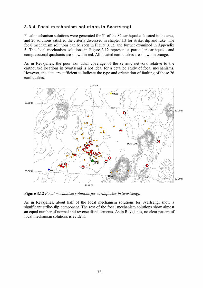
3.3.4 Focal mechanism solutions in Svartsengi
Focal mechanism solutions were generated for 51 of the 82 earthquakes located in the area, and 26 solutions satisfied the criteria discussed in chapter 1.3 for strike, dip and rake. The focal mechanism solutions can be seen in Figure 3.12, and further examined in Appendix 5. The focal mechanism solutions in Figure 3.12 represent a particular earthquake and compressional quadrants are shown in red. All located earthquakes are shown in orange.
As in Reykjanes, the poor azimuthal coverage of the seismic network relative to the earthquake locations in Svartsengi is not ideal for a detailed study of focal mechanisms. However, the data are sufficient to indicate the type and orientation of faulting of those 26 earthquakes.
Figure 3.12 Focal mechanism solutions for earthquakes in Svartsengi.
As in Reykjanes, about half of the focal mechanism solutions for Svartsengi show a significant strike-slip component. The rest of the focal mechanism solutions show almost an equal number of normal and reverse displacements. As in Reykjanes, no clear pattern of focal mechanism solutions is evident.

33
3.4 Results for the Fagradalsfjall area Fagradalsfjall is a 385 m high hyaloclastite table mountain on the Reykjanes Peninsula, making it the highest mountain on the peninsula (Sæmundsson and Einarsson, 1980). It is a product of a subglacial eruption, from the last part of the latest cold period of the ice age, which lasted about 100.000 years. A lava cap covers the highest, northwestern most part of the mountain, and recent lava flows surround the mountain.
Extensive surface fault mapping, as well as sub-surface fault mapping has been carried out in the Fagradalsfjall area (e.g. Sæmundsson and Einarsson, 1980; Clifton et al., 2003; Hjaltadóttir and Vogfjörð, 2006), where N-S striking, as well as NE- SW striking faults and fissures have been identified.
Seismic activity is common in the Fagradalsfjall area. In 1991-1996, when only one seismometer was installed on the Reykjanes Peninsula in Krýsuvík (station KRI), only 142 earthquakes were located in the Fagradalsfjall area (Hjaltadóttir and Vogfjörð, 2006). In 1996-1997, when six new seismometers were installed on the Reykjanes Peninsula, the sensitivity of the SIL network on the peninsula increased significantly (Jakobsdóttir, 1998). In comparison, around 5500 earthquakes were located in the Fagradalsfjall area between 1997 and 2005, with the largest earthquake swarms occurring in August 1998 (around 1300 earthquakes), in November 2000 (around 500 earthquakes) and in July 2004 (around 1900 earthquakes). These earthquakes have been analysed and used to map nearly 30 faults and fault-segments in the area (Hjaltadóttir and Vogfjörð, 2006).
Sigurlaug Hjaltadóttir (2009), used the relocated triggered earthquake distribution, induced by the large earthquakes on the 17th and 21st of June 2000 in the South Iceland Seismic Zone (SISZ), to map sub-surface fault planes in SW-Iceland, and to determine the slip distribution on them. A multi-event, relative relocation method was used to relocate the interactively located events. This method increased the location accuracy to such a degree that fault patterns, defined by the microearthquake distribution, were resolvable.
In the vicinity of Fagradalsfjall (Hjaltadóttir, 2009), most of the triggered earthquakes took place in the previously mentioned earthquake swarm in November 2000. The 2000 activity revealed a system of faults beneath the southwestern slopes of Fagradalsfjall striking N-S as well as NE-SW, in addition to two small clusters in the eastern slopes of the mountain striking N-S.
In general, most of the identified N-S and NE-SW striking sub-surface faults in the Fagradalsfjall area (Hjaltadóttir and Vogfjörð, 2006; Hjaltadóttir, 2009), show predominantly right-lateral strike-slip motion, as well as some faults with left-lateral strike-slip motion in between. Faults with a predominant normal component are also observed, as well as rare examples of faults with a predominant reverse component.

34
Figure 3.13 Earthquakes in the Fagradalsfjall area from December 2008 to May 2009,with E-W and N-S depth sections.
Earthquakes located with the SIL velocity model in the Fagradalsfjall area from December 2008 to May 2009 are shown in Figure 3.13. A total of 139 earthquakes were located, with the majority of earthquakes located beneath the southwestern slopes of Fagradalsfjall. A few earthquakes occurred to the northwest and to the east of the main seismic zone. The majority of the earthquakes located in the area (see Appendix 3) occurred between 5 and 8 km depth.
Average location uncertainties in latitude, longitude and depth were 620 m, 450 m and 1.070 m, respectively. The magnitudes of the earthquakes in Fagradalsfjall range from -0.3 to 3.0 ML with the majority of the earthquakes ranging from 0 to 1 ML (see Appendix 3).
3.4.1 An earthquake swarm in the Fagradalsfjall area
The majority of located earthquakes in the Fagradalsfjall area, or 133 of 139 earthquakes recorded, belong to one significant earthquake swarm located beneath the southwestern slopes of Fagradalsfjall (Figure 3.14). The earthquake swarm started at 15:35 on the 11th of February 2009, with two of the largest earthquakes of the swarm at the very beginning, at 18:35 and 18:38, of magnitude 2.13 ML and 3.03 ML, respectively. The earthquake swarm occurred during a three day period, with a total of 133 located earthquakes. The magnitudes of the earthquakes range from -0.09 ML to 3.03 ML, with the majority of the earthquakes ranging from 0 to 1 ML (see Appendix 3).

35
Figure 3.14 Selected earthquakes of the earthquake swarm in Fagradalsfjall in February2009, with E-W and N-S depth sections and the origin time of individual earthquakes.
Of the 133 located earthquakes of the earthquake swarm, 122 earthquakes were observed on either, or both, of the two stations to the east of the seismic activity, stations KAS and SAN, together with the twelve stations to the west of the seismic activity. As a constraint, these 122 earthquakes with the best azimuthal coverage were selected for further analysis and relative relocations.
36
The majority of the hypocentre locations of the earthquake swarm lie predominantly in a horizontal cluster at around 6 km depth, vertically elongated over a small depth range of 2 km, over an approximately 1 km2 area. A few of the hypocentre locations are around 1 km to the north of the center of the earthquake swarm, between 8 and 10 km depth.
Many of the events within the earthquake swarm exhibit similar seismic waveforms at multiple stations and identical P-wave first-motion polarities, as is evident e.g. on station NYL for multiple events (Figure 3.15). Waveform similarity and the epicentral clustering should suggest that the activity occurs on the same rupture plane with the same orientation and sense of failure.
This strong correlation of waveforms between events should not only confirm that the earthquakes are approximately co-located, but should also indicate that the focal mechanism solutions for the earthquakes must be similar and might even be identical.
However, slight differences in P-wave first-motion polarities were observed at multiple stations, which resulted in slightly different focal mechanism solutions to some degree (Figure 3.17).
3.4.2 Relative relocations of an earthquake swarm in the Fagradalsfjall area
A relative relocation of the earthquake swarm using a double-difference algorithm was made (Figure 3.15). Of the 122 selected earthquakes of the swarm, 120 earthquakes were relocated.
After relocating, the earthquake swarm reveals an approximately 1 km long N-S striking fault beneath the southwestern slopes of Fagradalsfjall, with the majority of events at around 5.9-7 km depth. Average location uncertainties in latitude, longitude and depth were 68 m, 40 m and 94 m, respectively. A few of the relocated earthquakes extend through the northern and southern end of the fault, and locate around 1 km to the north and south of the center of the earthquake swarm, at around 5-8 km depth to the north and around 5 km depth to the south.
The relative relocation of the swarm strengthens the postulate on the waveform similarity, which suggests the activity occurs on the same fault plane. The majority of events clearly occur on the same N-S striking fault plane.
The location of the N-S striking fault most likely corresponds to the location of a fault, or two fault segments believed to be one fault, mapped by Hjaltadóttir and Vogfjörð (2006). The southern fault segment was active in August, 1998, and forms a 700 m long lineament striking slightly east of north. The 33 earthquakes used to map the fault were located at 5.9-7.3 km depth, and focal mechanism solutions indicate a wide range of faulting mechanisms. The northern fault segment was active in November, 2000, and forms a 1500 m long lineament striking slightly east of north. The 177 earthquakes used to map the fault were located at 6.4-7.2 km depth, and focal mechanism solutions indicate predominantly right-lateral strike-slip motion, accompanied by a normal component.

37
Figure 3.15 Five seconds plots of vertical component traces for seven events of the earthquake swarm in the Fagradalsfjall area, observed at station NYL. All waveforms are bandpass-filtered between 4-40 Hz.

38
Figure 3.16 Relative relocations of the selected earthquakes of the earthquake swarm inFagradalsfjall in February 2009, with E-W and N-S depth sections and the origin time ofindividual earthquakes.
The majority of the relocated hypocentre locations of the earthquake swarm in this study lie predominantly in a horizontal cluster at around 6 km depth, vertically elongated over a small depth range of 1 km. These results are similar to the depth range of earthquakes used to map the previously mentioned fault by Hjaltadóttir and Vogfjörð (2006).
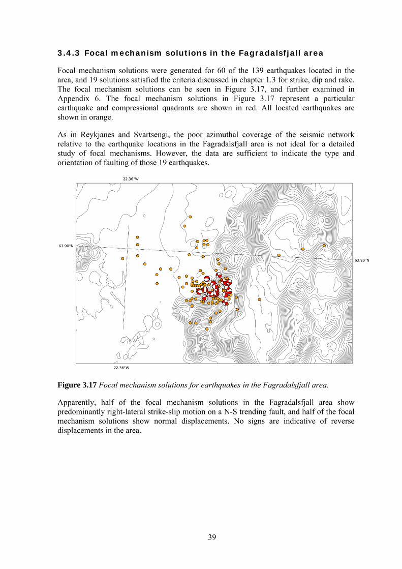
39
3.4.3 Focal mechanism solutions in the Fagradalsfjall area
Focal mechanism solutions were generated for 60 of the 139 earthquakes located in the area, and 19 solutions satisfied the criteria discussed in chapter 1.3 for strike, dip and rake. The focal mechanism solutions can be seen in Figure 3.17, and further examined in Appendix 6. The focal mechanism solutions in Figure 3.17 represent a particular earthquake and compressional quadrants are shown in red. All located earthquakes are shown in orange.
As in Reykjanes and Svartsengi, the poor azimuthal coverage of the seismic network relative to the earthquake locations in the Fagradalsfjall area is not ideal for a detailed study of focal mechanisms. However, the data are sufficient to indicate the type and orientation of faulting of those 19 earthquakes.
Figure 3.17 Focal mechanism solutions for earthquakes in the Fagradalsfjall area.
Apparently, half of the focal mechanism solutions in the Fagradalsfjall area show predominantly right-lateral strike-slip motion on a N-S trending fault, and half of the focal mechanism solutions show normal displacements. No signs are indicative of reverse displacements in the area.

40

41
4 Conclusions One of the specific topics of the European GEISER project (2010-2013), was analysis of induced seismicity from representative geothermal reservoirs throughout Europe. In the autumn of 2008, the energy company HS Orka hf. had planned an injection test in the Reykjanes geothermal field in Iceland. To increase the seismic sensitivity of the Icelandic regional seismic network (SIL) in the area during the test, and to be able to detect and locate eventual small size induced seismic events in Reykjanes, five temporary seismic stations were installed in December 2008, by the Institute of Earth Sciences at the University of Iceland. In addition, data from six SIL stations and three seismic stations operated by the University of Wisconsin were available for the same period.
The area under study encompassed mainly the western part of the Reykjanes Peninsula, i.e. the area west of longitude -22.4°, with the addition of the Fagradalsfjall area just east of the main study area. The injection test at Reykjanes was delayed, and the seismic stations of the University of Iceland had to be dismantled in the middle of May 2009, before full-scale injection started. However, small-scale injection was carried out in the Reykjanes geothermal field during the recording period, while more extensive injection was carried out in the Svartsengi geothermal field.
Seismic activity from December 2008 to May 2009 was less than on average in the study area, compared to the 17 years of available data from continuous monitoring of the SIL network. A total of 340 earthquakes and 40 explosions were located on the Reykjanes Peninsula and in its vicinity. In the area covered by the twelve westernmost seismic stations west of longitude -22.4°, 122 earthquakes were located, compared to only 20 earthquakes located by the SIL network alone. The temporary network of seismic stations, together with data from the six SIL stations, was successfully installed in order to detect smaller and consequently a larger number of earthquakes compared to the routine locations of the SIL network alone.
In the Reykjanes geothermal field, earthquake activity from December 2008 to May 2009 was low, with only a few earthquakes located within the production field and no indications of induced seismicity. The majority of the 23 earthquakes located in the area occurred between 2 and 5 km depth, with magnitudes ranging primarily from 0 to 1 ML. Average location uncertainties in latitude, longitude and depth were 420 m, 360 m and 650 m, respectively.
In the Svartsengi geothermal field, earthquake activity from December 2008 to May 2009 was noticeably greater than in the nearby geothermal field in Reykjanes, with a few earthquakes located close to the production field, and the majority of earthquakes located around and to the north of the injection boreholes, SV-17 and SV-24. As in Reykjanes, the majority of the 82 earthquakes located in the area occurred between 2 and 5 km depth, with magnitudes ranging primarily from 0 to 1 ML. Average location uncertainties in latitude, longitude and depth were 510 m, 370 m and 780 m, respectively. One significant earthquake swarm was located in vicinity of the injection boreholes on the 6th of March 2009. The earthquake swarm occurred during a five hour period, with a total of 29 located earthquakes. A double-difference relative relocation of the earthquake swarm provides spatial indications of induced seismicity.

42
In the Fagradalsfjall area, earthquake activity from December 2008 to May 2009 was mainly confined to one significant earthquake swarm located beneath the southwestern slopes of Fagradalsfjall. The majority of the 139 earthquakes located in the Fagradalsfjall area occurred between 6-8 km depth, with magnitudes primarily ranging from 0 to 1 ML. Average location uncertainties in latitude, longitude and depth were 620 m, 450 m and 1.070 m, respectively. The earthquake swarm occurred during a three day period from the 11th of February 2009, with a total of 133 located earthquakes. A double-difference relative relocation of the earthquake swarm reveals an approximately 1 km long N-S striking fault beneath the southwestern slopes of Fagradalsfjall, with the majority of events located at around 5.9-7 km depth. The location of the N-S striking fault, and the depth range of earthquakes used to map the fault, is similar to the location and the depth range of a fault, or two fault segments believed to be one fault, active in 1998 and 2000, mapped by Hjaltadóttir and Vogfjörð (2006). This earthquake swarm may have triggered an intense earthquake swarm that occurred in the Fagradalsfjall area in late May 2009, and subsequently the intense earthquake swarms that followed in the nearby Krýsuvík geothermal area during alternating periods of uplift and subsidence in 2009 and 2011 (Kristjánsdóttir, 2013).
The results of this study show that, in general, a dense seismic network increases the seismic sensitivity. The limitation of detecting small earthquakes relies upon several factors, including the noise level, seismic network geometry and the density of seismic stations. The noise level can be particularly high on the Reykjanes Peninsula with the ocean nearby and cliffs at the coastline. Still, by adding the temporary network, the sensitivity was increased by slightly less than one in magnitude, and the seismic network west of longitude -22.4° recorded around 10 times more earthquakes inside the network, compared to the SIL network, although it was focused on the plate boundary rather than the geothermal fields at Reykjanes and Svartsengi. In addition, the seismic activity on the westernmost part of the Reykjanes Peninsula is of episodic swarm character. Therefore, longer recording periods may be needed than in areas with more continuous background seismic activity.
Earthquake locations by the SIL network alone, west of longitude -22.4°, have considerably deeper hypocentres than our dataset located with the temporary network together with the SIL stations, although the same velocity model is used for earthquake locations in both cases. The depth estimation of the earthquakes west of longitude -22.4° is approximately 2 km shallower for 70% of located earthquakes using the temporary network together with the SIL stations, than using only the SIL network. This difference increases as the brittle-ductile boundary is approached. According to this study, the average brittle-ductile boundary west of longitude -22.4° is at 4.5-5.5 km depth, slightly shallower than suggested by Klein et al. (1973).
However, it should be kept in mind that this conclusion is based on a very small data set compared to the 17 years of available data from continuous monitoring of the SIL network. The majority of the SIL data are from a timespan prior to the installation and operation of the RNE station in Reykjanes in May 2008, when the depth resolution on the Reykjanes Peninsula was evidently much less. There is nothing that indicates that earthquake depths have been different during this recording period (i.e. December 2008 – May 2009), although it cannot be ruled out.

43
To manually check the depth difference of earthquakes located by the SIL network west of longitude -22.4°, compared with earthquakes located by the temporary network together with the SIL stations, 20 earthquakes of magnitude 0.8 ML or larger, observed on at least 3 of the 4 SIL stations west of longitude -22.4° during this recording period, were chosen for further analysis. On average, the earthquakes located 1.12 km shallower when only located with the available SIL stations than with the available stations of the temporary network together with the SIL stations. Therefore, the different earthquake depths can mainly be explained by the fact that a denser seismic network gives a much better depth determination.
Injection rates in the Reykjanes and Svartsengi geothermal fields are only available as average values per month while individual earthquake swarms may only last for a few hours as in the case of Svartsengi. As a consequence, no conclusions on the correlation between these observations in time can be drawn. Time of occurrence of seismic events is determined with an accuracy of more than 0.1 s. Therefore it is important for future seismic studies on induced events in geothermal areas that the injection rate is measured more frequently, preferably once every minute.
The use of the double-difference relative relocation method, to improve location accuracy of earthquake swarms in Svartsengi and Fagradalsfjall, has revealed localised activity close to the injection boreholes in Svartsengi, which has hitherto not been mapped, and a N-S striking fault beneath the southwestern slopes of Fagradalsfjall, which most likely corresponds to a fault that has been mapped before (Hjaltadóttir and Vogfjörð, 2006). However, the localised activity in Svartsengi was not enough to map any fault outlines.
Focal mechanism solutions for the located earthquakes in the Reykjanes and Svartsengi areas show that a wide range of faulting mechanisms characterizes the seismic activity in each area, with strike-slip, normal faulting and reverse faulting taking place. In the earthquake swarm on an apparent N-S striking fault beneath the southwestern slopes of Fagradalsfjall, focal mechanism solutions showed both right-lateral strike-slip motion and normal displacements, but no signs of reverse faulting. However, the poor azimuthal coverage of the seismic network relative to the earthquake locations in Reykjanes, Svartsengi and the Fagradalsfjall area is not ideal for a detailed study of focal mechanisms. The data are though sufficient to indicate the type and orientation of faulting of the located earthquakes.
The computer program, FPFIT, used to compute focal mechanism solutions (Reasenberg and Oppenheimer, 1985), assumes double-couple focal mechanism solutions, only considering pure shear motions on planar faults in isotropic elastic media, excluding any volume change at the source. Studies of complete moment tensor focal mechanism solutions show that microearthquakes in geothermal areas are often accompanied by volume changes at the source, which implies that these events involve processes more complicated than only pure shear faulting (Julian and Foulger, 2004). These volume changes correlate with exploitation activities in the geothermal areas. The wide range of faulting mechanisms observed in Reykjanes and Svartsengi might be explained by a component of volume increase, or decrease, not included in the double-couple focal mechanism solutions. Other possible explanations for different faulting mechanisms in approximately the same place at a similar time, e.g. in the Fagradalsfjall area, are that the earthquakes are caused by block faulting, or that they take place on non-optimally oriented faults.

44
Subsidence and pressure drawdown have been documented by levelling and gravity measurements in Reykjanes and Svartsengi throughout the years. The elliptical shape of subsidence in Reykjanes and Svartsengi is similar, elongated in the NE-SW direction, thus aligning with the trend of the normal faults and volcanic fractures in the area. In Reykjanes, results showed no sign of subsidence before the start of production, but then subsidence abruptly increased, and decreased again after the start of continuous injection (Magnússon, 2009). Similar for Svartsengi, the average rate of subsidence has decreased since full-time injection started in Svartsengi in 2001.
The low seismic activity located by the SIL network and other permanent seismic networks in Reykjanes and Svartsengi since the start of production, has been postulated to be the result of the fact that the subsidence and pressure drawdown may have increased the friction on potential fault planes, inhibiting fault slip, and thus reduced the microearthquake activity temporarily (Brandsdóttir et al., 2002; Keiding et al., 2010). The swarms located in both areas all seem to occur outside the boundary of the comparable elliptical shapes of subsidence. This explanation might apply to, to some extent, the low seismic activity located in Reykjanes and Svartsengi from December 2008 to May 2009.
In general, natural and induced earthquakes in a geothermal reservoir give important information on the status of the reservoir, e.g. stress conditions, flow pattern and physical properties. It is generally expected that induced earthquakes are of small magnitude. Therefore it is necessary to have sensitive networks to monitor the induced activity. One result of this study shows that noise is not a limiting factor for detection and a denser network will increase the sensitivity. For more reliable focal mechanism solutions, complete moment tensor inversion considering volume changes at the source should be done, instead of only double-couple focal mechanism solutions. Furthermore, to investigate induced seismicity in detail, a better time resolution of injection and production rates is needed.

45
References Aki, K. and P. G. Richards (1980). Quantitative Seismology, Theory and Methods, Vol. I. W. H. Freeman, San Francisco. Ágústsson, K., S. Th. Rögnvaldsson, B. H. Bergsson, and R. Stefánsson (1998). Jarðskjálftamælanet Veðurstofu Íslands og Hitaveitu Suðurnesja, VÍ-R98002-JA002 (in Icelandic). Ágústsson, K. and Ó. G. Flóvenz (2005). The thickness of the seismogenic crust in Iceland and its implications for geothermal systems in Iceland. Extended abstract, WGC 2005. Björnsson, G. and B. Steingrímsson (1992). Fifteen Years of Temperature and Pressure Monitoring in the Svartsengi High-Temperature Geothermal Field in SW-Iceland. Geothermal Resources Council Transactions, 16: 627-633. Brandsdóttir, B., H. Franzson, P. Einarsson, K. Árnason and H. Kristmannsdóttir (2002). Seismic monitoring during an injection experiment in the Svartsengi geothermal field, Iceland. Jökull, 51, 43-52.
Bjarnason, I. Th., W. Menke, Ó. G. Flóvenz and D. Caress (1993). Tomographic image of the Mid-Atlantic Plate Boundary in southwestern Iceland. J. Geophys. Res., 98, 6607-6622.
Böðvarsson, R., S. Th. Rögnvaldsson, R. Slunga and E. Kjartansson (1999). The SIL data acquisition system—at present and beyond year 2000. Phys. Earth planet. Inter., 113, 89–101. Clifton, A. E., C. Pagli, J. F. Jónsdóttir, K. Eyþórsdóttir, and K. S. Vogfjörð (2003). Surface effects of triggered fault slip on Reykjanes Peninsula, SW Iceland. Tectonophysics, 369, 145-154. DeMets, C. G., R. G. Gordon, D. F. Argus and S. Stein (1994). Effect of recent revisions to the geomagnetic reversal time scale on estimates of current plate motions. Geophys. Res. Lett., 21, 2191-2194. Einarsson, P. (1991). Earthquakes and present-day tectonism in Iceland. Tectonophysics, 189, 261-279.
Einarsson, P. (2008). Plate boundaries, rifts and transforms in Iceland. Jökull, 58, 35-58. Einarsson, P. and K. Sæmundsson (1987). Earthquake epicentres 1982-1985 and volcanic systems in Iceland (map), in Þorsteinn I. Sigfússon (ed.), Í hlutarins eðli: Afmælisrit til heiðurs Þorbirni Sigurgeirssyni prófessor. Menningarsjóður og Eðlisfræðifélag Íslands, Reykjavík. Einarsson, P. and S. Björnsson (1979). Earthquakes in Iceland. Jökull, 29, 37-43.

46
Einarsson, P. and S. Björnsson (1987). Jarðskjálftamælingar á Raunvísindastofnun háskólans, in Þorsteinn I. Sigfússon (ed.), Í hlutarins eðli: Afmælisrit til heiðurs Þorbirni Sigurgeirssyni prófessor. Menningarsjóður og Eðlisfræðifélag Íslands, Reykjavík (in Icelandic). Eysteinsson, H. (1999). Elevation and gravity changes at geothermal fields on the Reykjanes peninsula, SW-Iceland. Proceedings of the World Geothermal Congress 2000, 559-564. Japan.
Franzson, H., S. Þ. Guðlaugsson, G. Björnsson, J. Ö. Bjarnason and S. Þórhallsson (1999). Svartsengi - hola SJ-17: borun, rannsóknir og vinnslueiginleikar. Orkustofnun, report, OS-99036. 146 pp. (in Icelandic).
Franzson, H., 2000. Reykjanes high-temperature system. A study of fluid inclusions in wells RN-9 and RN-10. Orkustofnun, report OS-2000/021, 20pp. (In Icelandic).
Franzson, H., S. Thordarson, G. Björnsson, S. Guðlaugsson, B. Richter, G.Ó. Friðleifsson and S. Þórhallsson, 2002. Reykjanes high-temperature field, SW-Iceland. Geology and hydrothermal alteration of well RN-10. Workshop on Geothermal Reservoir Engineering, 27: 233-240.
Friðleifsson, G. Ó., H. Ármannson, K. Árnason, I. Þ. Bjarnason and G. Gíslason (2003). IDDP feasibility report. Iceland Deep Drilling Project, PART I, Geosciences – Site selection.
Friðleifsson, G. Ó., A. Albertsson, A. W. Elders, Ó. Sigurðsson, R. Karlsdóttir and B. Pálsson (2011). The Iceland Deep Drilling Project (IDDP): Planning for the Second Deep Well at Reykjanes. Geothermal Resources Council Transactions, 35: 347-354.
Guðnason, E. Á. and K. Ágústsson. (2014). Earthquake Swarm on Reykjanes in October 2013. Iceland GeoSurvey, ÍSOR-2014/017. 25 pp.
Halldórsson, P. (2011). Unpublished manuscript on historical earthquakes in Iceland.
Harðardóttir, V., K. L. Brown, Þ. Friðriksson, J. W. Hedenquist, M. D. Hannington and S. Þórhallsson (2009). Metals in deep liquid of the Reykjanes geothermal system, southwest Iceland: Implications for the composition of seafloor black smoker fluids. Geology, v. 37, no. 12, 1103-1106.
Hjaltadóttir, S., and K. S. Vogfjörð (2006). Kortlagning sprungna í Fagradalsfjalli á Reykjanesskaga með smáskjálftum. Kortlagning jarðhita í gosbeltum Íslands – Fyrsti áfangi, 2006. Icelandic Meteorological Office Report, 06001, VÍ-ES-01 (in Icelandic).
Hjaltadóttir, S. (2009). Use of relatively located microearthquakes to map fault patterns and estimate the thickness of the brittle crust in Southwest Iceland. Master’s thesis, Faculty of Earth Sciences, University of Iceland, pp. 104.
Jakobsdóttir, S. S. (1998). Uppsetning SIL-kerfisins. Icelandic Meteorological Office Report, VÍ-G98012-JA01.

47
Jakobsdóttir, S. S., G. B. Guðmundsson and R. Stefánsson (2002). Seismicity in Iceland 1991-2000 monitored by the SIL-system. Jökull, 51, 87-94.
Jóhannesson, H. and K. Sæmundsson (1999). Geological map of Iceland, 1:1.000.000. Iceland GeoSurvey.
Jónsson, J. T. and A. T. Guðmundsson (1968). Grunnhitamælingar á jarðhitasvæðinu á Reykjanesi (Ground temperature survey of the Reykjanes geothermal area at 50 cm depth). Orkustofnun.
Julian, B. R. and G. R. Foulger (2004). Microearthquake focal mechanisms. GRC Bulletin, July/August, 166-171.
Keiding, M., B. Lund, and Th. Árnadóttir (2009). Earthquakes, stress and strain along an obliquely divergent plate boundary: the Reykjanes Peninsula, southwest Iceland. J. Geophys. Res., 114, B09306.
Keiding, M., Th. Árnadóttir, S. Jónsson, J. Decriem and A. Hooper. (2010). Plate boundary deformation and man-made subsidence around geothermal fields on the Reykjanes Peninsula, Iceland. J. Volcanology and Geothermal Res., 194, 139-149.
Klein, F. W., P. Einarsson and M. Wyss (1973). Microearthquakes on the Mid-Atlantic plate boundary on the Reykjanes Peninsula in Iceland, J. Geophys. Res., 78, 5084-5099. Klein, F. W., P. Einarsson and M. Wyss (1977). The Reykjanes Peninsula, Iceland, earthquake swarm of September 1972 and its tectonic significance. J. Geophys. Res., 82, 865-888.
Kristjánsdóttir, S. (2013). Microseismicity in the Krýsuvík Geothermal Field, SW Iceland, from May to October 2009. Master’s thesis. Faculty of Earth Sciences, University of Iceland, pp. 50.
Le Meur, H., J. Virieux and P. Podvin (1997). Seismic Tomography of the gulf of Corinth: a comparison of methods. Annali di Geofisica, 40, 6, 1-24.
Lomax, A., J. Virieux, P. Volant and C. Berge (2000). Probabilistic earthquake location in 3D and layered models: Introduction of a Metropolis-Gibbs method and comparison with linear locations. In Thurber, C.H. and N. Rabinowitz (eds.), Advances in Seismic Event Location, 101-134, Kluwer, Amsterdam.
Magnússon, I. Þ. (2009). GNSS- og þyngdarmælingar á utanverðum Reykjanesskaga 2008. Iceland GeoSurvey, ÍSOR-2009/029. 62 pp. (in Icelandic).
Moser, T. J., T. van Eck and G. Nolet (1992). Hypocenter determination in strongly heterogeneous earth models using the shortest path method. J. Geophys. Res., 97, 6563-6572.
Podvin, P. and I. Lecomte (1991). Finite difference computation of traveltimes in very contrasted velocity models: a massively parallel approach and its associated tools. Geophys. J. Int., 105, 271-284.

48
Reasenberg, P.A. and D. Oppenheimer (1985). FPFIT, FPPLOT and FPPAGE: FORTRAN computer programs for calculating and displaying earthquake fault-plane solutions. U.S. Geol. Surv. Open File Rep. 85-739.
Sigmundsson, F. (2006). Iceland Geodynamics, Crustal Deformation and Divergent Plate Tectonics. Praxis Publishing – Springer Verlag, Chichester.
Sigurgeirsson, M. (1995). The Younger-Stampar eruption at Reykjanes, SW-Iceland. Náttúrufræðingurinn, 64, 211-230.
Sigurgeirsson, M. Á., O. Kjartansson, H. Björnsson, S. S. Jónsson and Christa Feucht (2008). Svartsengi - SV-24: borun holu SV-24. Iceland GeoSurvey, ÍSOR-2008/055. 61 pp. (in Icelandic).
Sæmundsson, K. (1978). Fissure swarms and central volcanoes of the neovolcanic zones of Iceland. Geol. J. Special Issue, 10, 415-432.
Sæmundsson, K. and S. Einarsson (1980). Geological map of Iceland, sheet 3, SW-Iceland, second edition, 1:250.000.
Sæmundsson, K. (1996). Svartsengi geological map, sheet 1, 1:25000. Orkustofnun, Hitaveita Suðurnesja and Landsvirkjun.
Tarantola, A. and B. Valette (1982). Inverse problems = quest for information. J. Geophys. Res., 50, 159-170.
The Icelandic Meteorological Office (2012). Downloaded 11. December 2012 from: http://hraun.vedur.is/ja/viku/.
The SeisComp seismological software (2013). Downloaded 12. October 2013 from: www.seiscomp3.org.
The U.S. Geological Survey (2013). Downloaded 10. October 2013 from: http://earthquake.usgs.gov/learn/topics/beachball.php.
Thordarson, T. and G. Larsen (2007). Volcanism in Iceland in historical time: Volcano types, eruption styles and eruptive history. J. Geodyn., 43, 118-152.
Tryggvason, E. (1968). Measurement of surface deformation in Iceland by precision levelling. J. Geophys. Res., 73, 7039-7050.
Tryggvason, E. (1970). Surface deformation and fault displacement associated with an earthquake swarm in Iceland. J. Geophys. Res., 75, 4407-4422.
Tryggvason, E. (1973). Seismicity, earthquake swarms, and plate boundaries in the Iceland region. Bull. Seis. Soc. Am., 63 (4), 1327-1348.
Tryggvason, A., S. Th. Rögnvaldsson and Ó. G. Flóvenz (2002), Three dimensional imaging of the P- and S-wave velocity and earthquake locations beneath Southwest Iceland. Geophys. J. Int., 151, 848-866.
49
Waldhauser, F. (2001). HypoDD: A computer program to compute double-difference hypocenter locations. U. S. Geol. Surv. Open File Rep. 01-113, 25 pp.
Waldhauser, F. and W. L. Ellsworth (2000). A double difference earthquake location algorithm: Method and application to the northern Hayward fault. Bull. Seism. Soc. Am., 90, 1353-1368.
Ward, P. and S. Björnsson (1971). Microearthquakes, swarms and the geothermal areas of Iceland. J. Geophys. Res., 76, 3953-3982.
Weir, N. R., R. S. White, B. Brandsdóttir, P. Einarsson, H. Shimamura, H. Shiobara and the RISE fieldwork team (2001). Crustal structure of the Northern Reykjanes Ridge and Reykjanes Peninsula, South-west Iceland. J. Geophys. Res., 106, 6347-6368.
Wessel, P. and W. H. F. Smith (1998). New improved version of generic mapping tools released. EOS Trans. AGU, 79(47), 579.
Wittlinger, G., G. Herquel and T. Nakache (1993). Earthquake location in strongly heterogeneous media. Geophys. J. Int., 115, 759-777.

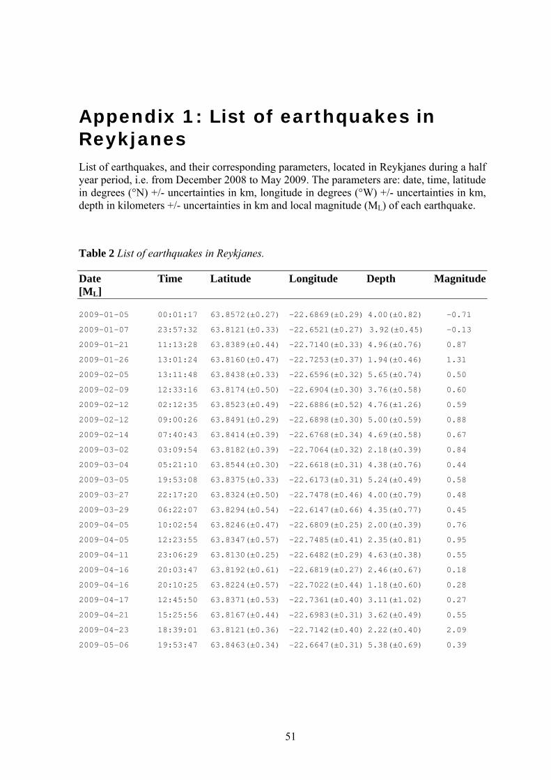
51
Appendix 1: List of earthquakes in Reykjanes List of earthquakes, and their corresponding parameters, located in Reykjanes during a half year period, i.e. from December 2008 to May 2009. The parameters are: date, time, latitude in degrees (°N) +/- uncertainties in km, longitude in degrees (°W) +/- uncertainties in km, depth in kilometers +/- uncertainties in km and local magnitude (ML) of each earthquake.
Table 2 List of earthquakes in Reykjanes.
Date Time Latitude Longitude Depth Magnitude [ML]
2009-01-05 00:01:17 63.8572(±0.27) -22.6869(±0.29) 4.00(±0.82) -0.71
2009-01-07 23:57:32 63.8121(±0.33) -22.6521(±0.27) 3.92(±0.45) -0.13
2009-01-21 11:13:28 63.8389(±0.44) -22.7140(±0.33) 4.96(±0.76) 0.87
2009-01-26 13:01:24 63.8160(±0.47) -22.7253(±0.37) 1.94(±0.46) 1.31
2009-02-05 13:11:48 63.8438(±0.33) -22.6596(±0.32) 5.65(±0.74) 0.50
2009-02-09 12:33:16 63.8174(±0.50) -22.6904(±0.30) 3.76(±0.58) 0.60
2009-02-12 02:12:35 63.8523(±0.49) -22.6886(±0.52) 4.76(±1.26) 0.59
2009-02-12 09:00:26 63.8491(±0.29) -22.6898(±0.30) 5.00(±0.59) 0.88
2009-02-14 07:40:43 63.8414(±0.39) -22.6768(±0.34) 4.69(±0.58) 0.67
2009-03-02 03:09:54 63.8182(±0.39) -22.7064(±0.32) 2.18(±0.39) 0.84
2009-03-04 05:21:10 63.8544(±0.30) -22.6618(±0.31) 4.38(±0.76) 0.44
2009-03-05 19:53:08 63.8375(±0.33) -22.6173(±0.31) 5.24(±0.49) 0.58
2009-03-27 22:17:20 63.8324(±0.50) -22.7478(±0.46) 4.00(±0.79) 0.48
2009-03-29 06:22:07 63.8294(±0.54) -22.6147(±0.66) 4.35(±0.77) 0.45
2009-04-05 10:02:54 63.8246(±0.47) -22.6809(±0.25) 2.00(±0.39) 0.76
2009-04-05 12:23:55 63.8347(±0.57) -22.7485(±0.41) 2.35(±0.81) 0.95
2009-04-11 23:06:29 63.8130(±0.25) -22.6482(±0.29) 4.63(±0.38) 0.55
2009-04-16 20:03:47 63.8192(±0.61) -22.6819(±0.27) 2.46(±0.67) 0.18
2009-04-16 20:10:25 63.8224(±0.57) -22.7022(±0.44) 1.18(±0.60) 0.28
2009-04-17 12:45:50 63.8371(±0.53) -22.7361(±0.40) 3.11(±1.02) 0.27
2009-04-21 15:25:56 63.8167(±0.44) -22.6983(±0.31) 3.62(±0.49) 0.55
2009-04-23 18:39:01 63.8121(±0.36) -22.7142(±0.40) 2.22(±0.40) 2.09
2009-05-06 19:53:47 63.8463(±0.34) -22.6647(±0.31) 5.38(±0.69) 0.39

52

53
Appendix 2: List of earthquakes in Svartsengi List of earthquakes, and their corresponding parameters, located in Svartsengi during a half year period, i.e. from December 2008 to May 2009. The parameters are: date, time, latitude in degrees (°N) +/- uncertainties in km, longitude in degrees (°W) +/- uncertainties in km, depth in kilometers +/- uncertainties in km and local magnitude (ML) of each earthquake.
Table 3 List of earthquakes in Svartsengi.
Date Time Latitude Longitude Depth Magnitude [ML]
2008-12-01 05:53:57 63.8512(±0.56) -22.5026(±0.49) 4.79(±0.68) 1.01
2008-12-16 03:05:29 63.8600(±0.42) -22.4462(±0.44) 2.97(±0.42) -0.04
2008-12-16 16:18:34 63.8625(±0.30) -22.5114(±0.28) 4.37(±0.39) 1.05
2008-12-16 16:20:45 63.8610(±0.32) -22.5166(±0.34) 3.86(±0.51) 0.07
2008-12-16 16:32:27 63.8622(±0.28) -22.5169(±0.28) 4.03(±0.44) 0.47
2008-12-16 16:35:25 63.8611(±0.26) -22.5144(±0.24) 4.42(±0.39) 0.22
2008-12-16 16:54:27 63.8614(±0.32) -22.5102(±0.39) 4.59(±0.48) -0.03
2008-12-30 14:05:33 63.8616(±0.31) -22.5194(±0.35) 2.82(±0.62) -0.53
2009-01-04 18:07:23 63.8838(±0.27) -22.4685(±0.31) 3.80(±0.59) -0.17
2009-01-04 18:08:53 63.8811(±0.83) -22.4648(±0.44) 4.31(±1.75) -0.88
2009-01-07 08:51:36 63.8648(±0.45) -22.4718(±0.33) 1.60(±0.59) -0.17
2009-01-11 09:08:59 63.8727(±0.51) -22.4851(±0.25) 0.28(±0.68) -0.06
2009-01-11 20:58:00 63.8607(±0.34) -22.4320(±0.17) 3.59(±0.45) -0.13
2009-01-12 01:31:34 63.8688(±0.38) -22.4752(±0.41) 1.70(±0.60) 0.17
2009-01-12 01:39:16 63.8628(±0.68) -22.4809(±0.26) 1.70(±0.70) -0.22
2009-01-13 07:48:22 63.8882(±0.64) -22.4292(±0.50) 0.91(±0.82) -0.40
2009-01-23 08:34:46 63.8779(±0.43) -22.3957(±0.38) 4.14(±0.71) 0.70
2009-01-29 08:05:50 63.8839(±0.27) -22.4699(±0.35) 3.80(±0.62) 1.37
2009-02-04 04:24:47 63.8653(±0.96) -22.4876(±0.42) 4.66(±1.36) 0.39
2009-02-04 06:38:32 63.8726(±0.58) -22.4861(±0.40) 3.90(±0.93) 0.55
2009-02-06 04:59:16 63.8593(±0.34) -22.4533(±0.37) 2.94(±0.35) 0.34
2009-02-10 15:42:12 63.8860(±0.57) -22.4382(±0.43) 1.49(±1.21) 0.32
2009-02-14 14:23:19 63.8848(±0.70) -22.4089(±0.65) 4.81(±1.82) 0.37
2009-02-22 14:33:49 63.8694(±0.27) -22.4699(±0.33) 2.52(±0.45) 0.82
2009-02-22 14:43:44 63.8777(±1.59) -22.4831(±0.47) 0.20(±1.27) 0.45
2009-03-06 04:50:19 63.8723(±0.31) -22.4861(±0.33) 3.80(±0.52) 1.26
2009-03-06 04:54:37 63.8797(±1.15) -22.4918(±0.35) 1.80(±1.28) 0.41
2009-03-06 05:12:13 63.8719(±0.99) -22.4972(±0.32) 2.80(±1.27) 0.41
2009-03-06 05:13:15 63.8828(±0.88) -22.4938(±0.36) 1.08(±1.26) 0.38

54
2009-03-06 05:14:20 63.8793(±0.85) -22.4925(±0.31) 1.80(±1.22) 0.43
2009-03-06 05:15:44 63.8712(±0.30) -22.4893(±0.31) 3.80(±0.50) 0.50
2009-03-06 05:17:36 63.8697(±0.28) -22.4843(±0.29) 3.96(±0.52) 0.57
2009-03-06 05:19:40 63.8688(±0.32) -22.4800(±0.32) 4.59(±0.48) 1.18
2009-03-06 05:22:09 63.8691(±0.32) -22.4801(±0.36) 5.14(±0.60) 0.77
2009-03-06 05:26:01 63.8857(±1.25) -22.4901(±0.48) 0.29(±1.65) 0.42
2009-03-06 05:27:24 63.8723(±1.01) -22.4940(±0.45) 3.01(±1.34) 0.39
2009-03-06 05:30:01 63.8703(±0.28) -22.4880(±0.28) 4.08(±0.50) 0.49
2009-03-06 05:34:05 63.8708(±0.28) -22.4885(±0.26) 3.86(±0.45) 0.53
2009-03-06 05:35:45 63.8708(±0.27) -22.4801(±0.30) 4.44(±0.46) 1.13
2009-03-06 05:42:21 63.8728(±0.31) -22.4841(±0.36) 3.85(±0.61) 0.55
2009-03-06 05:43:40 63.8684(±0.48) -22.4824(±0.41) 4.55(±0.74) 0.43
2009-03-06 05:46:58 63.8712(±0.31) -22.4795(±0.33) 4.52(±0.61) 0.68
2009-03-06 05:48:08 63.8737(±0.87) -22.4798(±0.30) 4.00(±1.64) 0.30
2009-03-06 05:49:49 63.8860(±1.24) -22.4870(±0.47) 0.22(±1.64) 0.40
2009-03-06 05:54:52 63.8776(±0.67) -22.4907(±0.25) 2.59(±1.16) 0.25
2009-03-06 05:59:05 63.8712(±0.29) -22.4803(±0.31) 4.45(±0.58) 0.49
2009-03-06 06:01:15 63.8691(±0.38) -22.4745(±0.35) 4.55(±0.73) 0.41
2009-03-06 06:12:08 63.8733(±0.39) -22.4878(±0.31) 3.76(±0.70) 0.43
2009-03-06 07:05:34 63.8734(±0.27) -22.4840(±0.30) 3.80(±0.47) 0.93
2009-03-06 07:31:15 63.8769(±0.88) -22.4986(±0.38) 2.39(±1.22) 0.38
2009-03-06 07:43:17 63.8748(±0.32) -22.4864(±0.33) 3.97(±0.50) 0.51
2009-03-06 07:58:49 63.8695(±0.33) -22.4817(±0.42) 4.52(±0.55) 0.64
2009-03-06 08:36:36 63.8888(±0.50) -22.4138(±0.37) 3.90(±0.91) 0.17
2009-03-06 08:45:50 63.8706(±0.27) -22.4960(±0.27) 3.39(±0.45) 0.50
2009-03-06 10:00:38 63.8677(±0.46) -22.4695(±0.55) 4.00(±1.28) 0.58
2009-03-29 17:43:48 63.8735(±0.56) -22.4730(±0.34) 4.26(±1.05) 0.45
2009-03-30 13:09:14 63.8673(±0.31) -22.5096(±0.28) 3.37(±0.45) 0.41
2009-04-08 20:40:33 63.8614(±0.33) -22.4891(±0.47) 1.88(±0.47) 0.49
2009-04-08 21:02:03 63.8682(±0.32) -22.4670(±0.37) 2.40(±0.49) 0.72
2009-04-08 21:28:47 63.8821(±0.27) -22.4657(±0.33) 4.17(±0.52) 1.08
2009-04-08 21:30:10 63.8897(±1.13) -22.4862(±0.46) 0.20(±1.48) 0.19
2009-04-08 21:33:32 63.8853(±0.98) -22.4821(±0.47) 1.70(±1.45) 0.29
2009-04-08 21:40:25 63.8811(±1.05) -22.4688(±0.45) 4.00(±1.76) 0.37
2009-04-09 01:57:31 63.8694(±0.26) -22.4755(±0.28) 1.67(±0.43) 0.70
2009-04-09 03:09:00 63.8650(±0.34) -22.4786(±0.25) 2.38(±0.45) 0.41
2009-04-09 10:59:32 63.8653(±0.38) -22.4604(±0.49) 1.46(±0.50) 1.60
2009-04-09 11:01:01 63.8689(±0.28) -22.4731(±0.37) 0.59(±0.42) 0.74
2009-04-09 11:02:47 63.8672(±0.37) -22.4563(±0.53) 1.51(±0.44) 0.79
2009-04-09 11:03:57 63.8675(±0.32) -22.4757(±0.46) 0.57(±0.53) 0.65
2009-04-09 11:06:19 63.8667(±0.43) -22.4734(±0.51) 0.56(±0.59) 0.62
2009-04-10 21:17:47 63.8827(±0.29) -22.4438(±0.39) 3.98(±0.57) 1.95

55
2009-04-10 21:18:56 63.8849(±0.54) -22.4525(±0.38) 3.80(±1.11) 0.33
2009-04-14 07:03:23 63.8683(±0.26) -22.5029(±0.25) 3.86(±0.43) 0.37
2009-04-14 07:25:48 63.8672(±0.35) -22.5106(±0.29) 3.37(±0.53) 0.48
2009-04-14 08:57:28 63.8680(±0.27) -22.5001(±0.27) 3.92(±0.44) 0.49
2009-04-14 09:10:57 63.8667(±0.42) -22.5045(±0.36) 3.45(±0.70) 0.49
2009-04-14 10:21:59 63.8675(±0.24) -22.5020(±0.26) 3.98(±0.42) 0.75
2009-04-23 21:00:55 63.8765(±1.21) -22.4770(±0.62) 0.19(±1.25) 0.58
2009-04-24 00:48:35 63.8765(±1.03) -22.4738(±0.64) 0.19(±1.06) 0.67
2009-05-10 00:39:16 63.8642(±0.36) -22.4084(±0.26) 1.11(±0.34) 1.10
2009-05-10 08:18:36 63.8741(±0.26) -22.4805(±0.27) 3.91(±0.43) 1.42

56

57
Appendix 3: List of earthquakes in the Fagradalsfjall area List of earthquakes, and their corresponding parameters, located in Fagradalsfjall during a half year period, i.e. from December 2008 to May 2009. The parameters are: date, time, latitude in degrees (°N) +/- uncertainties in km, longitude in degrees (°W) +/- uncertainties in km, depth in kilometers +/- uncertainties in km and local magnitude (ML) of each earthquake.
Table 4 List of earthquakes in the Fagradalsfjall area.
Date Time Latitude Longitude Depth Magnitude [ML]
2008-12-05 02:11:05 63.8970(±0.47) -22.2798(±0.39) 7.23(±1.11) 0.65
2009-01-25 21:06:17 63.8956(±0.57) -22.2900(±0.39) 9.09(±0.99) 0.87
2009-02-11 15:35:56 63.8893(±0.47) -22.3156(±0.46) 6.00(±0.95) 0.44
2009-02-11 18:35:05 63.8897(±0.39) -22.3125(±0.28) 6.03(±0.72) 2.13
2009-02-11 18:36:44 63.8918(±0.51) -22.3407(±0.68) 5.86(±1.12) -0.07
2009-02-11 18:38:16 63.8907(±0.42) -22.3126(±0.31) 6.03(±0.83) 3.03
2009-02-11 18:40:15 63.8907(±0.50) -22.3422(±0.65) 6.00(±1.07) -0.09
2009-02-11 18:42:01 63.8879(±0.41) -22.3235(±0.38) 6.03(±0.80) 0.27
2009-02-11 18:55:20 63.8904(±0.46) -22.3325(±0.56) 6.96(±0.94) 0.07
2009-02-11 18:56:51 63.8868(±0.46) -22.3161(±0.37) 6.82(±0.90) 0.24
2009-02-11 18:57:56 63.8851(±0.47) -22.3263(±0.41) 6.00(±0.83) 0.09
2009-02-11 19:00:22 63.8898(±1.08) -22.3249(±0.72) 6.80(±1.30) 0.21
2009-02-11 19:05:40 63.8941(±0.67) -22.3509(±0.82) 5.43(±1.48) 0.25
2009-02-11 19:08:54 63.8867(±1.19) -22.3173(±0.44) 6.08(±1.38) 0.37
2009-02-11 19:11:22 63.8891(±0.71) -22.3264(±0.52) 6.46(±1.20) 0.18
2009-02-11 19:31:25 63.8976(±0.73) -22.3226(±0.35) 8.87(±1.07) 0.54
2009-02-11 19:38:24 63.8900(±0.39) -22.3173(±0.30) 6.72(±0.95) 1.51
2009-02-11 19:48:19 63.8876(±0.61) -22.3122(±0.33) 6.51(±1.16) 0.82
2009-02-11 20:15:17 63.8858(±0.65) -22.3176(±0.40) 6.10(±1.16) 0.47
2009-02-11 20:29:09 63.8868(±0.53) -22.3105(±0.31) 6.00(±0.99) 0.65
2009-02-11 20:32:56 63.8893(±0.46) -22.3164(±0.35) 7.16(±0.94) 0.34
2009-02-11 20:39:48 63.8883(±0.45) -22.3211(±0.42) 6.31(±0.83) 0.40
2009-02-11 21:24:35 63.8830(±0.48) -22.3181(±0.43) 6.65(±0.84) 0.05
2009-02-11 21:30:06 63.8900(±0.38) -22.3133(±0.29) 6.24(±0.78) 1.55
2009-02-11 21:33:19 63.8858(±0.48) -22.3216(±0.50) 6.48(±0.92) 0.01
2009-02-11 21:36:45 63.8868(±0.47) -22.3209(±0.38) 6.03(±0.87) 0.18
2009-02-11 21:44:36 63.8865(±0.44) -22.3137(±0.31) 6.03(±0.86) 0.56
2009-02-11 21:49:32 63.8865(±0.49) -22.3265(±0.59) 6.03(±1.00) 0.07

58
2009-02-11 21:52:34 63.8907(±0.48) -22.3294(±0.61) 6.34(±1.05) 0.04
2009-02-11 21:57:09 63.8890(±0.48) -22.3252(±0.59) 6.44(±0.95) 0.01
2009-02-11 22:01:43 63.8904(±0.38) -22.3118(±0.28) 6.17(±0.74) 2.41
2009-02-11 22:03:16 63.8904(±0.46) -22.3269(±0.62) 6.48(±0.96) 0.05
2009-02-11 22:07:06 63.8900(±0.44) -22.3109(±0.32) 6.00(±0.86) 1.43
2009-02-11 22:13:59 63.8962(±1.10) -22.3256(±0.49) 6.05(±1.60) 0.33
2009-02-11 22:18:02 63.8919(±0.99) -22.3235(±0.50) 5.98(±1.66) 0.33
2009-02-11 22:21:58 63.8948(±1.01) -22.3287(±0.72) 6.05(±1.77) 0.18
2009-02-11 22:23:26 63.8921(±0.93) -22.3168(±0.32) 6.00(±1.43) 0.30
2009-02-11 22:25:06 63.8934(±1.30) -22.3573(±0.87) 5.70(±2.10) 0.11
2009-02-11 22:35:34 63.8976(±1.32) -22.3514(±0.92) 5.70(±2.21) 0.15
2009-02-11 22:44:31 63.8934(±1.04) -22.3157(±0.34) 5.98(±1.58) 0.33
2009-02-11 22:52:22 63.8891(±1.00) -22.3152(±0.35) 5.98(±1.53) 0.34
2009-02-11 22:55:16 63.8969(±0.85) -22.3225(±0.53) 5.77(±1.48) 0.62
2009-02-11 22:58:45 63.8946(±0.90) -22.3226(±0.35) 6.20(±1.42) 0.33
2009-02-11 23:03:06 63.8879(±0.47) -22.3266(±0.49) 7.30(±0.98) 0.07
2009-02-11 23:04:30 63.8883(±0.48) -22.3243(±0.57) 6.03(±0.99) 0.12
2009-02-11 23:11:09 63.8898(±0.47) -22.3265(±0.58) 6.25(±0.96) 0.08
2009-02-11 23:18:12 63.8879(±0.46) -22.3195(±0.41) 6.99(±0.91) 0.24
2009-02-11 23:19:42 63.8883(±0.50) -22.3235(±0.67) 7.03(±1.01) 0.07
2009-02-11 23:21:23 63.8819(±0.59) -22.3267(±0.65) 5.86(±1.22) 0.04
2009-02-11 23:33:41 63.8890(±0.51) -22.3268(±0.72) 6.03(±1.15) 0.08
2009-02-11 23:36:47 63.8893(±0.51) -22.3268(±0.66) 6.00(±1.14) 0.12
2009-02-11 23:42:40 63.8861(±0.49) -22.3121(±0.31) 6.03(±0.87) 0.68
2009-02-11 23:45:55 63.8907(±0.46) -22.3118(±0.32) 6.03(±0.93) 0.57
2009-02-11 23:47:18 63.8876(±0.46) -22.3162(±0.31) 6.61(±0.85) 0.20
2009-02-11 23:49:50 63.8893(±0.46) -22.3180(±0.34) 6.58(±0.87) 0.21
2009-02-11 23:52:15 63.8912(±0.40) -22.3155(±0.31) 7.01(±0.81) 0.68
2009-02-11 23:55:38 63.8893(±0.44) -22.3172(±0.44) 6.00(±0.90) 0.57
2009-02-11 23:57:59 63.8904(±0.43) -22.3142(±0.29) 6.96(±0.85) 0.47
2009-02-11 23:59:24 63.8890(±0.49) -22.3260(±0.64) 6.89(±1.00) 0.07
2009-02-12 00:02:57 63.8840(±0.47) -22.3158(±0.41) 6.00(±0.94) 0.24
2009-02-12 00:07:27 63.8883(±0.48) -22.3163(±0.35) 6.99(±0.94) 0.18
2009-02-12 00:12:00 63.8890(±0.45) -22.3252(±0.55) 6.41(±0.90) 0.12
2009-02-12 00:19:44 63.8886(±0.51) -22.3131(±0.35) 6.03(±1.03) 0.59
2009-02-12 00:22:11 63.8879(±0.72) -22.3179(±0.39) 6.34(±1.06) 0.39
2009-02-12 00:24:53 63.8861(±0.57) -22.3216(±0.52) 6.00(±1.00) 0.11
2009-02-12 00:30:51 63.8890(±0.47) -22.3236(±0.47) 5.89(±0.92) 0.07
2009-02-12 00:36:08 63.8883(±0.47) -22.3219(±0.31) 6.55(±0.93) 0.23
2009-02-12 00:42:03 63.8872(±0.59) -22.3106(±0.33) 6.03(±1.13) 0.40
2009-02-12 00:43:34 63.8884(±0.47) -22.3231(±0.50) 6.94(±0.92) 0.08
2009-02-12 00:45:59 63.8877(±0.47) -22.3166(±0.32) 6.18(±0.87) 0.23

59
2009-02-12 00:47:18 63.8876(±0.48) -22.3194(±0.46) 6.27(±0.91) 0.11
2009-02-12 00:50:13 63.8849(±0.59) -22.3067(±0.80) 5.98(±1.24) 0.05
2009-02-12 00:53:17 63.8861(±0.48) -22.3153(±0.41) 5.89(±1.02) 0.55
2009-02-12 00:57:34 63.8893(±0.48) -22.3156(±0.30) 6.75(±0.94) 0.62
2009-02-12 00:59:45 63.8844(±0.52) -22.3142(±0.41) 5.89(±1.03) 0.23
2009-02-12 01:03:53 63.8883(±0.62) -22.3179(±0.38) 6.48(±0.96) 0.43
2009-02-12 01:12:13 63.8881(±0.47) -22.3239(±0.53) 6.36(±0.93) 0.14
2009-02-12 01:22:26 63.8876(±0.44) -22.3186(±0.41) 6.03(±0.82) 0.33
2009-02-12 01:23:43 63.8900(±0.46) -22.3181(±0.31) 6.72(±0.88) 0.27
2009-02-12 01:29:26 63.8890(±0.45) -22.3212(±0.45) 6.65(±0.87) 0.07
2009-02-12 01:33:50 63.8904(±0.48) -22.3269(±0.63) 6.03(±1.06) 0.02
2009-02-12 01:36:45 63.8897(±0.47) -22.3221(±0.52) 6.65(±0.91) 0.24
2009-02-12 01:40:21 63.8872(±0.47) -22.3210(±0.30) 6.86(±0.91) 0.23
2009-02-12 01:42:02 63.8904(±0.48) -22.3205(±0.41) 6.61(±0.88) 0.21
2009-02-12 01:43:11 63.8891(±0.46) -22.3216(±0.40) 7.15(±0.87) 0.25
2009-02-12 01:51:12 63.8895(±0.51) -22.3176(±0.38) 7.18(±0.97) 0.24
2009-02-12 01:57:02 63.8900(±0.48) -22.3181(±0.41) 6.03(±0.89) 0.17
2009-02-12 01:59:13 63.8858(±0.56) -22.3192(±0.32) 6.00(±1.07) 0.30
2009-02-12 02:07:36 63.8883(±0.60) -22.3107(±0.39) 6.03(±1.12) 0.44
2009-02-12 02:08:40 63.8876(±0.43) -22.3154(±0.32) 6.44(±0.77) 0.92
2009-02-12 02:19:30 63.8879(±1.14) -22.3219(±0.57) 6.48(±1.24) 0.31
2009-02-12 02:21:42 63.8858(±0.48) -22.3160(±0.37) 6.96(±0.95) 0.46
2009-02-12 02:23:14 63.8883(±0.52) -22.3123(±0.33) 6.00(±0.90) 0.62
2009-02-12 02:32:55 63.8865(±0.66) -22.3249(±0.55) 5.89(±1.09) 0.27
2009-02-12 02:46:42 63.8914(±0.93) -22.3223(±0.52) 6.96(±1.12) 0.36
2009-02-12 02:48:32 63.9002(±0.88) -22.3313(±0.50) 8.51(±1.09) 0.20
2009-02-12 02:50:57 63.8865(±0.82) -22.3145(±0.42) 6.03(±1.24) 0.46
2009-02-12 03:04:03 63.8890(±0.58) -22.3116(±0.33) 6.55(±1.11) 0.50
2009-02-12 03:06:12 63.8861(±0.51) -22.3177(±0.37) 6.03(±0.97) 0.27
2009-02-12 03:10:47 63.8942(±0.89) -22.3162(±0.31) 6.00(±1.42) 0.65
2009-02-12 03:38:01 63.8969(±2.06) -22.3209(±0.40) 5.77(±2.00) 0.66
2009-02-12 03:40:42 63.8969(±1.25) -22.3209(±0.43) 5.63(±1.78) 0.41
2009-02-12 04:04:05 63.8879(±0.42) -22.3235(±0.36) 6.72(±0.81) 0.31
2009-02-12 04:06:56 63.8900(±0.50) -22.3149(±0.32) 7.03(±0.95) 0.30
2009-02-12 04:17:27 63.8893(±1.05) -22.3196(±0.41) 7.68(±1.10) 0.44
2009-02-12 04:22:30 63.8926(±0.66) -22.3476(±0.81) 5.70(±1.39) -0.02
2009-02-12 04:25:54 63.8925(±0.48) -22.3128(±0.33) 6.51(±0.92) 0.47
2009-02-12 04:29:12 63.8974(±0.57) -22.3254(±0.38) 8.88(±0.94) 0.27
2009-02-12 04:31:02 63.8876(±0.56) -22.3098(±0.34) 6.00(±1.07) 0.43
2009-02-12 04:34:53 63.8879(±0.49) -22.3179(±0.38) 7.13(±0.94) 0.30
2009-02-12 04:44:32 63.8858(±0.56) -22.3112(±0.40) 6.44(±1.04) 0.33
2009-02-12 04:47:59 63.8893(±0.48) -22.3228(±0.44) 6.44(±0.94) 0.14

60
2009-02-12 04:53:24 63.8861(±0.57) -22.3224(±0.48) 6.00(±0.96) 0.11
2009-02-12 04:55:49 63.8872(±0.46) -22.3170(±0.31) 7.44(±0.90) 0.31
2009-02-12 04:58:04 63.8890(±0.47) -22.3244(±0.44) 6.96(±0.91) 0.33
2009-02-12 05:07:34 63.8891(±0.49) -22.3168(±0.34) 6.73(±0.97) 0.57
2009-02-12 05:22:18 63.8962(±0.65) -22.3512(±0.76) 6.25(±1.38) 0.01
2009-02-12 05:33:41 63.8877(±0.61) -22.3182(±0.46) 6.53(±1.01) 0.28
2009-02-12 05:50:40 63.9020(±0.76) -22.3291(±0.45) 8.57(±1.01) 0.37
2009-02-12 06:00:23 63.8977(±0.47) -22.3214(±0.33) 7.68(±0.94) 0.50
2009-02-12 06:08:32 63.8872(±0.58) -22.3178(±0.44) 6.82(±0.95) 0.36
2009-02-12 06:37:28 63.8823(±0.62) -22.3180(±0.66) 5.82(±1.13) 0.21
2009-02-12 07:00:26 63.8872(±1.41) -22.3074(±0.37) 6.55(±1.34) 0.47
2009-02-12 07:04:00 63.8893(±1.08) -22.3292(±0.63) 6.86(±1.18) 0.34
2009-02-12 07:15:27 63.8861(±0.45) -22.3177(±0.30) 6.99(±0.86) 0.43
2009-02-12 07:27:32 63.8876(±0.46) -22.3186(±0.41) 6.82(±0.91) 0.39
2009-02-12 08:43:06 63.8893(±0.72) -22.3212(±0.47) 6.03(±1.11) 0.37
2009-02-12 09:24:31 63.8919(±1.11) -22.3363(±0.77) 5.98(±1.40) 0.47
2009-02-12 12:31:24 63.8868(±0.83) -22.3153(±0.40) 6.00(±1.23) 0.66
2009-02-12 13:29:33 63.8883(±0.53) -22.3131(±0.36) 6.65(±1.02) 0.40
2009-02-13 06:48:07 63.8890(±1.12) -22.3419(±0.74) 5.86(±1.47) 0.53
2009-02-13 06:50:29 63.8861(±1.10) -22.3288(±0.47) 6.03(±1.25) 0.50
2009-02-13 09:07:07 63.8879(±0.57) -22.3155(±0.37) 6.03(±1.12) 0.68
2009-02-13 15:06:01 63.8886(±0.44) -22.3307(±0.50) 6.65(±0.85) 0.37
2009-02-14 21:32:16 63.8861(±0.45) -22.3272(±0.43) 6.03(±0.81) 0.30
2009-03-23 14:12:13 63.8809(±0.47) -22.3194(±0.32) 6.00(±0.89) 0.47
2009-03-28 20:48:46 63.8870(±0.49) -22.2974(±0.32) 6.05(±0.99) 0.65
2009-04-12 08:49:33 63.8819(±0.47) -22.3243(±0.37) 5.86(±1.10) 0.28
2009-04-16 14:04:33 63.8979(±0.73) -22.2707(±0.52) 9.11(±1.23) -0.34

61
Appendix 4: Focal mechanism solutions in Reykjanes
Focal mechanism solutions, as plotted by FPFIT, for earthquakes located in Reykjanes from December 2008 to May 2009.

62
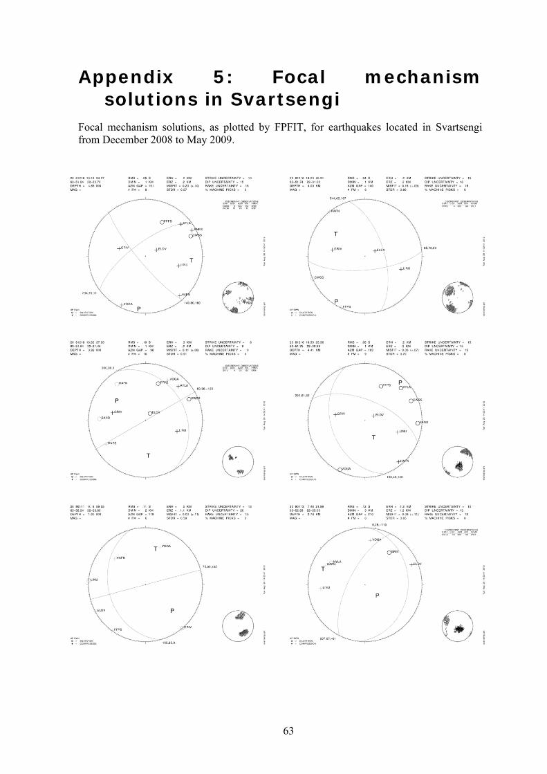
63
Appendix 5: Focal mechanism solutions in Svartsengi
Focal mechanism solutions, as plotted by FPFIT, for earthquakes located in Svartsengi from December 2008 to May 2009.

64

65

66
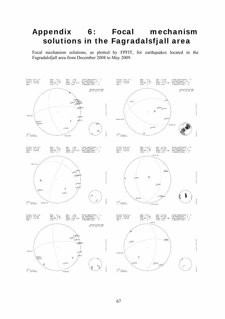
67
Appendix 6: Focal mechanism solutions in the Fagradalsfjall area
Focal mechanism solutions, as plotted by FPFIT, for earthquakes located in the Fagradalsfjall area from December 2008 to May 2009.

68

69


![Crustal stress field in southern California and its ... angles, with the FPFIT software package [Reasen- berg and Oppenheimer, 1985]. All events have location uncertainties of _•1](https://static.fdocuments.in/doc/165x107/5aafdfdb7f8b9a22118dc036/crustal-stress-field-in-southern-california-and-its-angles-with-the-fpfit-software.jpg)


