ANALYSIS OF ROBUST ORDER STATISTICCFAR DETECTORS

BY

DANIEL T. NAGLE

Submitted in partiai fuilfiilment of therequirements for the degree of

Doctor of Philosophy in Electrical and Computer Engineeringin the School of Advanced Studies of

iliinois Institute of Technoiogy

Approved

Chicago, I l l inois

\'{av, 1991

Advisor

ACKNOWLEDGEMENT

This work was created through the assistance of many people. I wish to thank

my friend and academic advisor of seven years, Dr. Jafar Saniie, for the opportunity

to work with him and for giving me the focus and the motivation to accomplish this

work. I would like to thank my defense committee members: Dr. E. Olsen, Dr. D.

Ucci, and Dr. G. Atkin for their interest and their insightful discussions. Also, I

thank Dr. Kevin Donohue for his participation, insights, and friendship.

I wish to acknowledge the Office of Naval Research and the Energy Power

Research Institute for their support throughout my graduate studies.

Finally, I have many family members and friends which have encouraged me

and strengthened my spirit throughout this endeavor. My dearest thanks go to my

father and grandmother for their unbelievable devotion and confidence in my goals.

D.T.N.

l l l

TABLE OF CONTENTS

ACKNOWLEDGMENTPage

l l t

vi

ix

xi

L IST OF TABLES

LIST OF FIGURES

\BSTRACT

( .HAPTERI. INTRODUCTION

Statistical Signal Detection Theory 2Nonparametric and Distribution-Free Signal Detection....... 4Basic CFAR Detector... 7

1.3.1 Radar Applications.... . . . . . . 81.3.2 Statistical Models for Radar .. 11

CFAR Threshold Estimation 15Generalized CFAR Design .. 18

1.5.1 Maximum Likelihood CFAR Detectors. 241.5.2 Analysis of the CA-CFAR Detectors .. . . . . . . . . . 311.5.3 Threshold Statistics of ML and

CA-CFAR Detectors. 331.6 Order Statistics 4l1.7 Outline of Present Research Goals 421.8 Preview of Remaining Chapters... . . . . . . . . 43

il. BACKGROUI\D THEORY

2.1 Statistical Properties of Order Statistics2.2 Estimation Properties of Order Statistics

2.2.1 Order Statistics Stemming from an UniformDist r ibut ion . . . . . . . . . . . . . .

2.2.2 Order Statistics for General ClutterDis t r ibut ions. . . . . . . . . . . . .

2.2.3 Asymptotic Estimation Properties of OrderStatistics

2.2.4 Summary.... . . . .2.3 Nonparametric Applications of Order Statistics2.4 Previous Work in the Field of Nonparametric

CFAR Detectors

l . l1.21.3

1.41.5

46

4658

727474

lv

CHAPTERm.

Page

84

IV.

NONPARAMETRIC ANALYSIS OF OS-CFARDETECTORS

3.1 Unmodified OS-CFAR Detector 873.1.1 Asymptotic UOS-CFAR Performance.... . . . . . . 91

3.2 Scaled OS-CFAR Detector... 923.2.1 Asymptotic Analysis of SOS-CFAR Detector... . . . . . . 1013.2.2 Statistical Properties of SOS-CFAR Threshold...... 105

3.3 Generalized OS-CFAR Detectors 1073.3.1 One-Parameter OS-CFAR

Detector... 1103.3.2 Asymptotic Design of the One-Parameter

OS-CFAR Detectors Il23.3.3 Weibulll One-Parameter OS-CFAR I)etector:

Unknown Shape Parameter 1133.4 Mult iple Parameter OS-CFAR Detector Design... 118

3.4.1 Weibull Two-Parameter OS-CFARDetector Design.... . . I20

3.4.2 Asymptotic Analysis of WTPOS-CFARDetector... L26

3.4.3 Statistics of WTPOS-CFAR ThresholdEstimate 128

3.5 Censored Maximum Likelihood CFAR Detector 1313.5.1 Asymptotic Analysis of Threshold Estimate........... I343.5.2 Statistics of Threshold Estimate 135

3.6 Trimmed-Mean CFAR Detector... 1373.6.1 Asymptotic Analysis of Threshold Estimate........... 1403.6.2 Statistics of Threshold Estimate.. 144

3.7 Best Linear Unbiased CFAR Detectors. 1483.7.1 Asymptotic Analysis of Threshold Estimate........... 1573.7.2 Statistics of Threshold Estimate 159

AI{ALYSIS OF ROBUSTNESS OF OS-CFAR DETECTORS... 167

4.1 Probability of Detection Analysis of OS-CFAIIDetectors 168

4.2 Asymptotic Probability of Detection Analysis I724.3 Performance of OS-CFAR Detectors under Lehmann's

Alternative Hypothesis... . . . . . . . . . I734.3.1 Pp of UOS-CFAR Detector . . . . . . . . . . . . . L754.3.2 PD of SOS-CFAR Detector . . . . . . . . . . . . . 1754.3.3 PD of CML-CFAR Detector . . . . . . . . . . L794.3.4 PD of TM-CFAR Detector .. . . . . . . . . . . . 1794.3.5 PD of BLU-CFAR Detector . . . . . . . . . . . . . . L824.3.6 Performance Comparisons of OS-CFAR Detectors L82

CHAPTER

APPENDIXA.B .C .D .

REFERENCES

Page4.4 Performance of OS-CFAR Detectors for Chi-Squared

Distributed Target-Plus-Clutter 1844.5 Performance of WTPOS-CFAR Detector 1954.6 Performance of OS-CFAR Detectors for Inhomogenous

KNS. . . . . . . . . 2034.7 Summary of OS-CFAR Detectors Performance.... . . . . . . . . . . . . . . . . 2L3

V. CONCLUSIONS

Contributions of OS-CFAR Detectors AnalysisOS-CFAR Detector Applications.... . . . . . . . . .Extensions of this Research..

5.15.25.3

217

2172r8220

CFAR BIAS FOR THRESHOLD ESTIMATESASYMPTOTIC OPTIMALITY OF ML-CFARCONVERGENCE OF RELATIVE RANKSBLUE COEFFICIENTS FOR EXPONENTIALLY

DISTRIBUTED OBSERVATIONSE. PDFS OF OS-CFAR THRESHOLD STATISTICS

DETECTOR.. . . .222225227

229232

v i

LIST OF TABLES

Table3.1 Accuracy of BLUE Coefficients

Page

153

v l l

LIST OF FIGURES

Figure Page1.1 Graphical Binary Detection Problem 51.2 Basic CFAR Detection Problem... I1.3 Radar Detection System 10L.4 Various Weibull pdfs... . . . . . . . 131.5 Weibull ML-CFAR Performance for Ideal Scaling.... . . . . . . . . . . 291.6 Scaling for Weibull ML-CFAR Detectors with a: 10-3... . . 30L.7 Required Scaling for Weibull CFAR Detectors with a =, 10-3 341.8 Eff iciency of ML verses CA Estimates.... . . . . . . . . 351.9 (a) Normalized ADT and (b) Normalized Threshold Variance

of CA and ML-CFAR Detectors... . . . . . . 371.10 Normalized MSE of CA and ML-CFAR Detectors... . . . . . 391.11 Performance of Exponentially-Designed CA-CFAR Detectors 402.L Sor t Funct ions for n :5. . . . . . . . . 482.2 (a) Sort Functions and (b) Output pdfs for Input

Observations, tr. . . . . . . . . 502.3 Example of an Inverse CDF with a superimposed

sort function for n:25 512.4 (a) MSE and (b) Normalized MSE of U-Statist ics .. . . . . . . . . 612.5 Various pdfs and Inverse CDF with

Normalized Power (Znd Moments) ........ 632.6 Bias of (a) OS Quantile Estimates a1d (b) Normalized

OS Quanti le Estimates for order ,. . . . . . . . . . . . . . . 642.7 Bias of (a) OS Quantile Estimates and (b) Normalized

OS Quanti le Estimates for order t ' . . . . . . . . . . . . . 662.8 Variance of (a) OS Quantile Estimates and (b) Normalized

OS Quanti le Estimates for order t. . . . . . . . . . . . . . . 682.9 MSE of (a) OS Quantile Estimates a1d (b) Normalized

OS Quanti le Estimates for order t. . . . . . . . . . . . . . . 702.IO MSE of (a) OS Quantile Estimates and (b) Normalized

OS Quanti le Estimates for order t ' . . . . . . . . . . . . . 7L2.ll Asymptotic Normalized Variance (a) by a factor L and

(b) bv a factor v-Fo ' ( t ) . . . . . . . . . . . . . . 73

2.L2 Basic CFAR DetectJr System 772.13 CA-CFAR Detector System.... . 792.14 GO & SO-CPAR Detector System.. . . . 812.15 General OS-CFAR Detector System .. 823.1 Ppl o f UOS-CFAR for severa l n . . . . . . . . . . . . . . . 903.2 Graphic Translation of Scaled OS-CFAR Threshold 94

V l l l

Figure3.33.4J . O

3.6

t nJ . l

Page

Pps of SOS-CFAR Detector with Various Scaling 98

Ppl o f SOS-CFAR Detector for c : 1 , 1 .5, 2 . . . . . - . . . . . . . ' . 99

Scaling factor o' of SOS-CFAR Detector for given n... . . . . . . . . . . . LOz

(u) Pr,q, Performance of SOS-CFAR with Ideal Scaling, and (b)

Asymptotic (Ideal) and Actual Scaling Factor a for a:0.001 ..... 104

Normalized Asymptotic Threshold Variance for SOS-CFARDetector 106

3.8 Normalized ADT of SOS-CFAR Detector for Weibull Distributions.. 108

3.9 Normalized (a) Variance and (b) MSE of SOS-CFAR Detector... . . . . . . . 109

3.10 Ideal Design Exponent Parameter for CFAR-Detector Ll4

3.11 Ppl for Exponent Design Parameter .. 116

3.12 Actual Exponent Design Parameter for CFAR-Detector LL7

3.13 Ppl for Fixed Design Parameter of WTPOS-CFAR Detector 124

3.L4 Design Parameter d for WTPOS-CFAR Detector for n:25 125

3.15 (a) Ideal Design Parameter 0r for WTPOS-CFAR Detector *and (b) Ppl of WTPOS-CFAR Detector Designed Using 0 ......' 127

3.16 Normalized (a) ADT and (b) Variance of WTPOS-CFAR Detectorfor c:1 129

3.LT Normalized (a) ADT and (b) Variance of WTPOS-CFAR Detector

for c:2 130

3.18 Normalized (a) ADT, (b) Variance, and (c) MSE for CML-CFAR

Detector 136

3.19 Design Parameter d for TM-CFAR Detector... . . . . . . . I4l

3.2O Ideal Scaling Factor 0' for TM-CFAR Detector... I43

3.2L Asymptotic Normalized Variance of Threshold for TM-CI'AR

Detector L45

3.22 Normalized ADT of TM-CFAR Detector for Various n... . . . . . ' . . . . . . . . . . . . . L47

3.23 Normalized Threshold Variance of TM-CFAR Detector forVarious Values of n... . . . . . . . 149

3.24 Normalized Threshold MSE of TM-CFAR Detector forVarious Values of n... . . . . . . . 150

3.25 Numerical Errors In the Linear Solution of theBLU Est imate. . . . . . . . . . . . . . 154

3.26 Asymptotic Variance of BLU Threshold Estimate 160

3.27 Asymptotic Efficiency of TM w.r.t. BLUThreshold Estimates 161

3.28 Normalized ADT of BLU-CFAR Detector for Various n... . . . . . . . . . . . . ' . . . . . L62

3.29 Normalized Threshold Variance of BLU-CFAR Detector forVar ious Values of n . . . . . . . . . . 163

3.30 Normalized Threshold MSE of BLU-CFAR Detector forVar ious Values of n . . . . . . . . . . 164

3.31 Eff iciency Tlu,uB,r, for Various Values of n... . . . . . . . 165

TX

PageFigure4.1 Comparisons between /1(r) and ADT, T ... . . . . . . . . . . . 1704.2 Graphical Definit ion of CFAR Loss.... . . . . . . 1744.3 Performance of UOS-CFAR Detector 1764.4 Optimal Neyman Pearson Detector Performance............. L774.5 CFAR Loss of SOS-CFAR Detector for a:0.001.... . . . . 1784.6 CFAR Loss of CML-CFAR Detector for a:0.001 1804.7 CFAR Loss of TM-CFAR Detector for a :0.001. . . . . . . . . 1814.8 CFAR Loss of BLU-CFAR Detector for o:0.001 1834.9 Comparisons of CFAR Loss of One-Sided Censoring OS-CFAR

Detectors for Lehmann's Hypothesis (n:5) 1854.lO Comparisons of CFAR Loss of One-Sided Censoring OS-CFAR

Detectors for Lehmann's Hypothesis (n:25) 1884.Ll Comparisons of CFAR Loss of TweSided Censoring OS-CFAR

OS-CFAR Detectors for Lehmann's Hypothesis (n=,5) 1914.I2 Comparisons of CFAR Loss of TwoSided Censoring OS-CFAR

Detectors for Lehmann's Hypothesis (n:25) 1934.13 Comparisons of CFAR Loss of One-Sided Censoring OS-CFAR

Detectors for Chi-Squared Target-Plus-Clutter (n:5) 1964.I4 Comparisons of CFAR Loss of One-Sided Censoring OS-CFAR

Detectors for Chi-Squared Target-Plus-Clutter (n:25) 1984.15 Comparisons of CFAR Loss of Two-Sided Censoring OS-CFAR

Detectors for Chi-Squared Target-Plus-Clutter (n:5) 2OO4.16 Comparisons of CFAR Loss of Two-Sided Censoring OS-CFAR

Detectors for Chi-Squared Target-Plus-Clutter (n:)5) 2O24.L7 Performance of WTPOS-CFAR Detector for Exponentially

Distr ibuted Clutter Compared with BLU-CFAR Detector.. 2044.18 Performance of WTPOS-CFAR Detector for Rayleigh-Distributed

Clutter Compared with CML & SOS-CFAR Detectors... . . . . . . . . . . . . . 2064.I9 Performance of WTPOS-CFAR Detector for Rayleigh-Distributed

Clutter Compared with Exponentially DesignedCML & SOS-CFAR Detectors. 2OB

4.2O Performance of SOS-CFAR Detector for Inhomogeneous KNS.... . . . . . . . zLI4.2I Performance of TM-CFAR Detector for Inhomogeneous KNS 2124.22 Performance of BLU-CFAR Detector for Inhomogeneous KNS.... . . . . . . 2144.23 Performance Comparisons of OS-CFAR Detectors

for Inhomogeneous KNS.... . . . . . 2I55.1 Split-Spectrum Processing Block Diagram z[g

ABSTRACT

Constant False Alarm Rate (CFAR) detectors have been utilized in radar

systems where the clutter environment is partially unknown and/or has varying

statistical properties (e.g., power, etc.). ln such instances, the performance of a

fixed optimal detector deteriorates significantly, and nonparametric or CFAR

detector is designed to be invariant to changes in the clutter density function. An

effective method of accomplishing this is to use local estimates for the threshold

from a set of known noise or clutter samples (KNS) related to the unknown (or

varying) parameters of the clutter distribution. However, the problem arises where

the KNS contains target information which will significantly degrade the probability

of detection.

Recently, Order Statistics (OS) and Trimmed-Mean (TM) processors have been

utilized to obtain robust estimates of the threshold in the presence of

inhomogeneous clutter observations for exponential clutter distributions. These

techniques, however, do not fully utilize the a priori information related to the

clutter distribution resulting in degradation in the probability of detection.

Furthermore, the study of OS-based threshold estimators designed under the CFAR

constraint is applicable to other clutter distributions.

In this thesis, general derivations of OS-CFAR detectors are given for assumed

'rarametric variations. The OS-CFAR threshold estimate is derived in order to

allow for the detector's performance to be invariant from the given distribution

:rarameter. Several OS-CFAR detectors are considered, where either one or more

,)rder statistics are used to estimate a single parameter. In particular, explicit

.olutions are obtained where the clutter has a Weibull distribution with unknown

-cale. In order to improve the performance of the OS and TM-CFAR detectors,

::rore efficient threshold estimates are examined, i.e., the Censored Maximum

.-ikelihood (CML) and Best Linear Unbiased (BLU) estimators of the scale

.)arameter of Weibull clutter distributions.

In addition, multiple order statistics can be used to estimate several parameters

i rhe clutter distribution and can be applied to the CFAR det,ection problem.

x i

General constraints similar to the one-parameter OS-CFAR detector are derived.

The Weibull Two Parameter Order Statistic (WTPOS) CFAR detector is examined

to account for variations in both the scale and shape parameters of the Weibull

clutter distribution. It is shown through performance results how these different

OS-CFAR detectors can be used most effectively and how they perform with

respect to one another.

Performance comparisons are based on examining the statistics of the CFAR

threshold estimate and the probability of detection performance under Lehmann's

alternative hypothesis. Since smaller threshold values indicate better detection

performance at a given CFAR level, the BLU and CML-CFAR detectors show

better target detection where the contamination of the clutter observations is small.

However, in the case of extreme contamination, the TM-CFAR detector is shown to

perform more robustly for exponentially-distributed clutter. The performance of

these one-parameter invariant OS-CFAR detectors are also compared with the

WTPOS-CFAR detector. It is shown that limited improvement in robustness can

be obtained for the WTPOS-CFAR detector. This is due to the lack of efficiency of

the WTPOS threshold estimate. Thus, this work facilitates a general

nonparametric (or invariance) design of several types of OS-CI'AR detectors and

illustrates their performance characteristics for different degrees of KNS

contamination.

x l l

CHAPTER I

INTRODUCTION

ln detection systems (e.g. radar), the effects of interfering signals (clutter) from

the environment a.re usually partially unknown and/or varying in terms of their

statistical properties. In such insta,nces where the performance of the optimal

detector deteriorates significantly, Constant False Alarm (CFAR) detectors can be

used since they are insensitive to changes in the underlying statistics of the

clutter. In recent years, order statistics have found many applications in CFAR

radar [Wei82,Roh83,Don87,Won87,Gan88], and have been utilized extensively for

over the pa.st four decades in nonparametric statistics ISch45,Leh53,Fra57,

Har65a,Che67]. Particularly, the use of ranks of ordered observations have

dominated most of the nonparametric techniques in statistics. The main objective

of this thesis is to analyze the effectiveness of using order statistics in general

threshold estimation producing adaptive detection systems of a nonparametric

nature. The performance of these adaptive detectors are evaluated using common

radar target and clutter models.

ln this chapter, basic detection theory is presented with emphasis on error

analysis and performance criteria. Nonparametric and Distribution-Free

performance criteria are defined and several Constant False Alarm Detector

|CFAR) designs are discussed. The CFAR detector is introduced where the

threshold is estimated to accommodate nonstationary clutter environments. The

mucimum likelihood threshold estimate is analyzed in terms of efficiency and

performance in the CFAR detector and an example given for Weibull distributed

clutter. These estimation techniques are shown to be very sensitive to outliers;

accordingly, more robust estimators are examined. The order statistic is

introduced for the purpose of censoring data in such a fashion that deviations

(outliers) from certain regions of the underlying distribution are ignored. Finally,

an outline of research goals and an overyiew of the following chapters is given.

l.l Statistical Signal Detection Theory

Statistical decision theory used in such fields a.s radar, sonar, digital

communication, and ultrasonic imaging, attempts to discriminate between

information bearing signals a"nd noise or interference. For the binary detection

problem, the observations can be classified in two mutually exclusive sets: the

null hypothesis, .[16, consisting of noise (clutter) samples, and the alternative

hypothesis, Hr, consisting of the signal (target) and noise. In deciding between

the two hypothesis two types of errors can occur: (type I error) //r is accepted

when 116 is true which is referred to a.s a false-alarm, md (type II error) I/6 is

accepted when 111 is true referred to as a miss. These errors are of course

inherently dependent upon the statistical models of the two hypotheses and the

design of the detector.

In classical detection theory, the probability distribution functions of the two

hypotheses are either assumed or known a priori. From these functions the design

of the detector can be found from the Bayes likelihood ratio [BayI764]. For the

given o priori density functions of the random variable X and an observed value,

z, the form of the optimum detector is given by likelihood ratio, L(r):

Py(r I H1)L l r ) :

P - ( r l l h )(1 .1 )

where Px@ | 111) and Px@ | //6) are the conditional probability densities of X, at

z, given events .[/1 and IIe, respectively. A decision is made by comparing the

test statistic, L(x), to a threshold, ), which is related to the performance of the

detector.

L(r) I , ^I < )t -

arcept H1

accept l/6(1.2)

ln general, when the equality holds, a random decision rule can be employed which

is generally equiprobable between the two hypotheses but may be biased depend-

ing upon the performance criteria of the detector and/or the cost associated with

each hypothesis [Van68]. As for now, the equality is set for Hs to minimize the

probability of a false acceptance of .I/1 which is critical as discussed below.

The threshold determines the performa.nce of the detector in terms of the two

errors previously discussed by fixing either the probability of false alarm or the

probability of miss. It is often the case that the occurrence of false ala.rm is of fa^r

greater concern than the occurrence of a miss. This is a practical consideration

since the ramifications of the accepting the hypothesis .E[1 can be very critical.

Thus, the choice of a threshold ) for the optimum detector must be evaluated

according to the constraints on the probability of false alarm of the detector.

The probability of false alarm, PFA, can be found by the Neyman-Pearson cri-

teria.

PFA : I*^ , (t (r) | Hs)d,L < d for all r (1 .3)

where a is a fixed quantity referred to as the size of the detector. This means

that for all observations, r, the probability of false alarm is guaranteed not to

exceed a. This type of optimizing constraint is also termed constant folse olarm

rote (CF LR) analysis. This will be the optimization constraint for the different

detectors considered in this thesis. It should be noted that no information about

the target is used in deciding the threshold which means this detector will not

have the same probability of detection performance for different target distribu-

tions.

Though the probability of type I error is guaranteed to be below a given level,

a, over all observations belonging to the null hypothesis, I/6, the type II error is

governed by the statistics of the alternative hypothesis, Ht. The probability of

miss (type II error), P14 can be calculated by evaluating the integral of the test

statistic in Equation 1.2 over the region specified by the threshold, ), that is,

)P u : I r Q @ ) l H ) d L ( n ) : L - 0

-oo

where 1 - B corresponds to the probability of a miss. The probability of detection,

Pp, simply corresponds to B in which the integral in the above equation is

(1.4)

evaluated over the complementary region, (),oo], of probability of a miss. A

graphical representation of the Py and Ppl is shown in Figure 1.1. As can be

seen, the probability of detection is determined by the threshold ) (chosen to

satisfy the CFAR constraint) which is pre-ordained by the statistics associated

with the null hypothesis. This implies that the performance of a detector (in terms

of probability of detection) with fixed size, a, cannot be improved independently

of the statistics of the target.

The analysis so far has briefly outlined the steps that would be taken to make

an optimal decision in the insta^nce where the designer ha.s complete statistical

knowledge of the hypotheses (i.e., the conditional probability density functions).

However, this incalculable good fortune rarely occurs in reality. In practical detec-

tion systems, such as radar, assumptions are made in order to model an environ-

ment which can be subject to change with time (e.g., clouds, birds, pollution,

chaffes, etc.). These changes can degrade the performance of the detector consid-

erably. Thus, the performance of the detector is optimal only as long as the

underlying assumptions concerning the environment and the target a.re valid. In

the following sections, alternative optimization procedures are described in which

the detector is designed under loose assumptions about the densities of the two

hypotheses.

1.2 Nonparametric and Distribution-Free Signal Detection

Constant false alarm techniques and nonparametric techniques have been used

synonymously in the past literature [Dil71,Kas80,Wei82,Rol83,Web85,Ga^n88] to

describe detectors which are insensitive to statistical variations in the null

hypothesis. That is to say the detector can be designed with a probability of false

alarm bound, a, while assuming limited a priori statistical information about the

observations under the null hypothesis. In the past literature, several definitions of

''nonparametric test," "nonpalametric hypothesis," and "nonparametric detector"

exist [Dil71,Haj69,Gib71,Kas80,Fras57,Leh53] which vary the generality of the dis-

tributions belonging to the null hypothesis. In this study, the definition of a non-

BASIC BINARY DETECTION PROBLEM

holdThres

t\ i

(u=

(!

, /

' ( x l H 1 )

Figure 1.1 Graphical Binary Detection Problem

Observation x

parametric detector is aligned with [Dil71] where the assumptions on the statistics

of the observations belonging to the null hypothesis pertain only to the form of the

distribution function (e.g., Lognormal, Weibull, Gamma, etc.) and set no fixed

parametric values in determining the type I error. A formal definition of a non-

pa.rameter detector is given below [Dil71]:

Giuen the clutter has a density function, /o (";@), and, distribution F6 (r;O) where

@ rs o linite set of paTorneters, a detector is nonparometric if the probobility ol

false olarm maintains o giuen performance bound (size a) when the parameter(s)

of the probabitity density function, @ under the null hypothesis, Ho, vory ouer oll

allowable ualues.

The design procedure for the nonparametric detector is difficult since optimiza-

tion is accomplished over a class of distributions belonging to the null hypotheses

(referred to as a composite hypothesis in contrast to the simple hypothesis in the

previously section). For a composite hypothesis characterizedby parametric vari-

ations in O, the optimal detector design is given by the Uniformly Most Powerlul

(UMP) detector [Leh59,Fra57,Haj69] which will perform as well as if the

parameter(s) @ were known. Thus, the likelihood ratio and the threshold of Equa-

tions 1.1 and 1.2 must be evaluated independent of O. In most ca.ses, however,

the UMP detector can not be found in which case plausible or justifiable but

suboptimal design procedures are utilized.

A common alternative detector design used is the generalized likelihood ratio

Van68] where maximum likelihood estimates of unknown parameters are used in

the likelihood ratio. This is intuitively satisfying since the maximum likelihood

estimate is optimal over a class of unbiased estimators. Despite this, the form of

the generalized likelihood ratio may not guarantee CFAR performance indepen-

dent of the actual value of the unknown parameters. An example of a non-

parametric generalized likelihood detector will be shown later for the Weibull

clutter distribution with unknown scaling parameter.

If the detector is designed with far looser constraints than the previously

defined nonpararnetric case where the form of the detector was not assumed, then

the detector is termed distribution-free. The term distribution-free implies that

the performance of the detector for type I and type II error is independent of the

underlying distributions of the hypotheses. The difference between the two

hypotheses is generally cha.racterized as a shift or scale transformation in the dis-

tribution function. In almost all these distribution-free tests, however, some mild

conditions a.re required which are usually imposed on the distributions of the

hypotheser (".g., symmetry, zero mean, etc.) [Leh53,Fra57,Gib71] or require the

availability of some observations stemming from the null hypothesis known o

p r i o r i IS av66,D il 7 l,Dil7 41.

Suboptimal nonparametric or distribution-free detectors are designed either to

extract the information present in the observations in order to account for the gap

of missing a priori knowledge of the distribution for the null hypothesis or to focus

on specific differences between the hypothesis (e.g., median, variance, etc). Note

that the term "suboptimal" is in respect to the Bayes detector where the o priori

distribution of the observation belonging to the null hypothesis is assumed known.

When a priori information is incomplete or changing, the nonparametric detector

will perform more robustly compared to the Bayes detector since it adapts to the

local statistics of the observations. Furthermore, the nonpa^rametric and

distribution-free detectors are popular because they are often simpler to imple-

ment than parametric models and have relatively acceptable loss of power (proba-

bility of detection performance) compared to the optimal detector [Kas80]. Thus,

the motivation for using these techniques is to compensate for lack of a priori

knowledge in the two hypotheses or obtain CFAR performance which is invariant

over some composite hypothesis.

1.3 Basic CFAR Detector

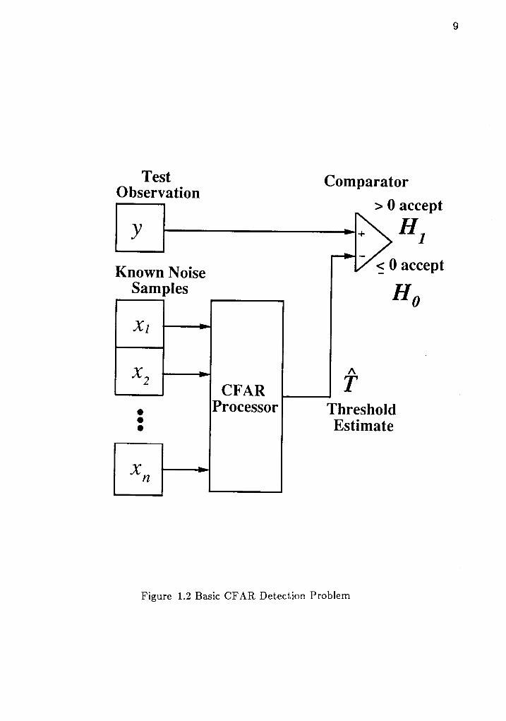
The CFAR detection system considered here consists of determining if a single

rest observation belongs to either Hs or H1 using a set of noise observations

belonging to 1/6) referred to as the Known Noise Samples (KNS) [Dil71]. The

KNS are used to estimate a threshold for the test observation. A schematic of this

detector is shown in Figure 1.2 where y corresponds to the test observation of the

received signal and the vector r : {rr,82, ..., rn} corresponds to the KNS. The

procurement of the known noise samples presents many interesting challenges

which are discussed in Chapter fV and V in terms of practical implementations of

this detector. The basic premise of this one-sample detector is to utilize a set of

null observations to discriminate whether or not a test sample belongs to 116 or

,[/1 under the CFAR performance constraint.

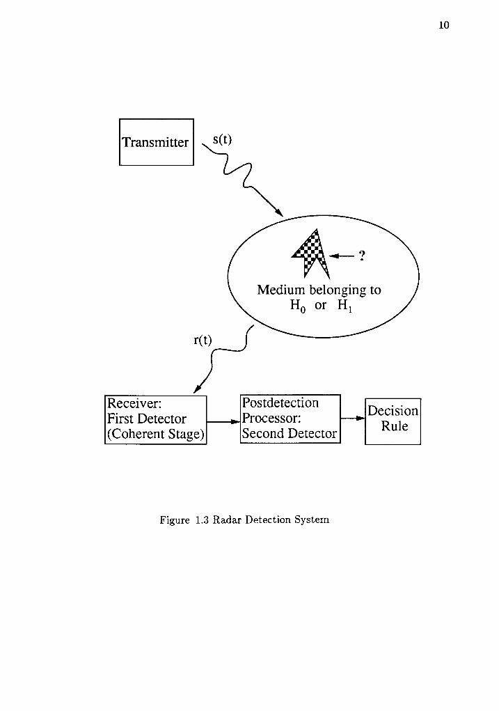
1.3.1 Radar Applications. In this section, several basic rada.r systems are

introduced and the acquisition of tests samples and KNS a.re discussed. The radar

system basics are shown in Figure 1.3 where the transmitted signal s (t) is modu-

lated through media of hypothesis l{ producing the received signal r(t). The

received signal then goes to the first detector (coherent detector) which may con-

sist of a linear envelope detector, square-law detector, or a matched filter [DiF80].

This stage retrieves amplitude features which may be related to the target's pres-

ence (position and velocity) corresponding to either a test observation, y, or KNS,

r. The second stage is referred to as the postdetection processor (incoherent

detection) in which a decision is ultimately made. The aforementioned CFAR

detector is a postdetection processor which processes the amplitude information of

a single test cell given a set of n known noise samples.

There are several types of radar transmission systems where the observations

can be acquired from the received signal(s) over time and/or frequency. The most

comnon types of radar systems are fixed frequency pulse radar, phased array

radar [DiF80l, frequency agile radar, and frequency diversity radar [Van74,Ray66].

The simplest of these is the fixed frequency pulsed radar system where n

pulses at the same center frequency are transmitted from one radiating source at a

specified rate, referred to as the pulse repetition frequency (p.f), in order to irradi-

ate a target within a given observation time. The observation time is dependent

on how much time can be spared to keep the antenna focused in one direction or

in the case where the antenna rotates at a uniform rate the prf is determined from

I

TestObservation

Known NoiseSamples

Comparator

> 0 accept

HI

< 0 accept

Ho

nT

ThresholdEstimate

CFARProcessor

Figure 1.2 Basic CFAR Detection Problem

10

Transmitter

Medium belonging toHo or Hl

PostdetectionProcessor:econd Detector

Receiver:First Detector(Coherent Stage)

Figure 1.3 Radar Detection System

1 1

the a,ntenna beam-width and the rotation rate.

In a phased-array radar system, several radiating elements with different

phases are used to focus the energy of the beam in a specific direction. The

received signals are then scaled appropriately and added together coherently to

emphasize the energy of the beam profile in a specific direction [Dif80]. The major

advantage over the fixed frequency pulse radar is that the antenna does not have

to move and finer resolution may be obtained. In both these ca.ses the test obser-

vations and/or noise observations are obtained sequentially over time.

Effective techniques for detecting targets in stationary noise are frequency agil-

ity [Bea68] and frequency diversity [Gua68]. Clutter decorrelation is achieved by

simultaneously transmitting with two or more channels centered at different fre-

quencies (frequency diversity), or by shifting the transmitted frequency between

pulses (frequency agility). The received signals a.re then processed over time and

frequency pa.ssing amplitude information to the postdetection processor. These

techniques are also useful in detecting targets with small cross sectional a.reas since

the wavelength of the pulses are changing and will consequently have a better

chance of hitting the target at a good aspect.

1.3.2 Statistical Models for Radar. The statistical modeling of the two

hypotheses is a vast research topic with numerous types of distributions con-

sidered [Nat67]. Basically, the models are chosen to satisfy some a.ssumptions

about the backscattering elements under the clutter and target-plus-clutter

hypotheses. If the clutter is composed of many scatterers where no single one is

dominant and the number of scatterers are large enough such that the central

limit theorem holds, then the received signal r(t) can be viewed a.s a narrowband

Gaussian channel with uniform phase [Van68,Ker51]. The corresponding distribu-

tion of the postdetection (incoherent) observations corresponding to the linear

envelope detector have a Rayleigh distribution [Dif80,Van68] given by:

f x @ ) : \ " - t , l d ' f o r r ) op '

(1.5)

L2

where pl is the scale parameter associated with the power of the signal s(t) given

by (s2(t)>: pz12. If a matched filter [Dif80] or square-law detector [Swe57] is

used in the coherent stage, then the output incoherent observations will be

exponentially-distributed as follows IWei82]:' t -z lp

f x @ ) - : e f o r 2 2 0 (1.6)

where the power of the input signal corresponds to <t2(t)):F. In some

instances, the above assumptions on clutter are not valid and empirical models

\at67] are needed to describe the distribution. The Weibull distribution which

incorporates Equations 1.5 and 1.6 is given by:

(1.7)

rvhere c is the shape parameter which allows for larger or smaller tails in the den-

sity function. This can be seen in Figure 1.4 where several Weibull density func-

: ions with unity power are plotted for c:0.8, 1.0, 2.O,and2.2.

Modeling of the distribution of the received signal amplitude, U, (assuming a

.inear envelope detector for Figure 1.3) under the alternative hypothesis has been

generalized into four cases by Swerling [Swesa]. Cases one and two correspond to

:he target-plus clutter distribution modeled as Rayleigh distribution of Equation

1.5. Cases three and four model the target-plus-clutter a.s a Chi distribution given

i r \ ' :

, -@ lD 2

r ( " ) (1 .8)

rr.here 2u represents the degrees of freedom which is set to four (u:2)

:iwe54,Dif80]. Note that if a square law or matched filter is used as the coherent

detector the distributions of the observation y will change resulting in exponen-

r ially distributed observations for Swerling Cases I and II and Chi-Squa"red distri-

buted observations for Swerling Cases III and IV. The Chi-Square density func-

tion is given by:

| ' l c - l

f x@) : ! l z l r -@ld ' ro , "<oP l t ' l

t 1 2 v - l) | r l

f x k ) : t l = |p l t ' )

13

0 . 5 1 1 . 5 2 2 . 5

Weibull Probabiliw Densiw Functions

Figure 1.4 Various Weibull pdfs

l4

-x l l t

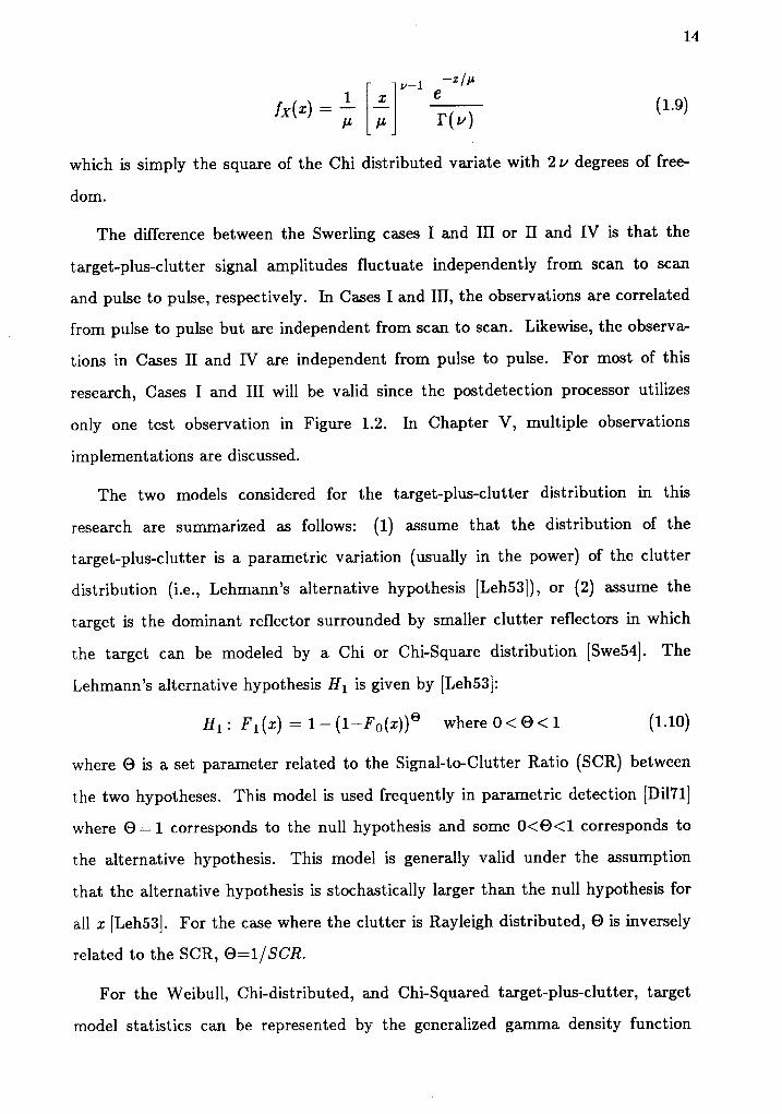
fx@)| \ v -I r lt - lL t ' )

distribu

I: -Lr

(1.e)r ( " )

which is simply the square of the Chi

dom.

ted variate with 2 u degrees of free-

The difference between the Swerling cases I a^nd III or II and tV is that the

target-plus-clutter signal amplitudes fluctuate independently from scan to scan

and pulse to pulse, respectively. In Cases I and III, the observations a.re correlated

from pulse to pulse but are independent from scan to scan. Likewise, the observa-

tions in Cases II and fV are independent from pulse to pulse. For most of this

resea,rch, Cases I and III will be valid since the postdetection processor utilizes

only one test observation in Figure 1.2. In Chapter V, multiple observations

implementations are discussed.

The two models considered for the target-plus-clutter distribution in this

research are summarized as followsr (1) a.ssume that the distribution of the

target-plus-clutter is a parametric variation (usually in the power) of the clutter

distribution (i.e., Lehmann's alternative hypothesis [Leh53]), or (Z) a.ssume the

target is the dominant reflector surrounded by smaller clutter reflectors in which

the target can be modeled by a Chi or Chi-Square distribution [Swesa]. The

Lehmann's alternative hypothesis y'/1 is given by [Leh53]:

H 1 : F 1 ( " ) : t - ( t - f o 1 r ; ) e w h e r e 0 < O < 1

where O is a set parameter related to the Signal-toClutter Ratio (SCR) between

the two hypotheses. This model is used frequently in parametric detection [Dil71]

where O:l corresponds to the null hypothesis and some 0(O{1 corresponds to

the alternative hypothesis. This model is generally valid under the assumption

that the alternative hypothesis is stochastically larger than the null hypothesis for

all r [Leh53]. For the case where the clutter is Rayleigh distributed, O is inversely

related to the SCR, @:LlSCR.

For the Weibull, Chi-distributed, and Chi-Squared target-plus-clutter, target

model statistics can be represented by the generalized garnma density function

(1.10)

15

lSta65l:

| 1 c v - rc l x l- t - tt L l t ' l

,-@ lD '

with corresponding F x@),

Fx@): re (v) l t (r) ' (1.11b)

where €:(rltt) c and I(') is the Gammafunction [ArbO ]. The moments of the

generalized garnma distribution function are given by:

n ( v c + m )' l ' J

fx@) :

nlx^l: I r* fx@) d,x : tr '- 0

r ( " ) (r . t ta)

(1 .1 l c )

These target models are utilized in Chapter fV in the robust analysis of CFAR

detectors. For the remainder of this research, the analysis is geared towards the

general cases where the clutter is assumed to have a Weibull distribution, and the

:arget-plus-clutter is assumed to have a generalized gamma distribution.

1.4 CFAR Threshold Estimation

In the design of a CFAR detector, the effectiveness of the threshold estimate is

,. haracterized by the statistics indicating how concentrated the sample estimate is

:o the ideal CFAR threshold. The ideal CFAR threshold, ?, for the one-sample

:est is given by:

T : F o L ( t - " ) ( 1 .12)

',r'here tr'01 ( ') is the inverse distribution function for the null hypothesis and a is

: he fixed probability of false alarm of the CFAR detector. Since tr'tt ( ' ) is not

inown a priori, the null observations, 3, are used to create an estimate of the

:hreshold, ?(z) as shown in Figure 1.2. If the observations are a.ssumed home

geneous, ,t"--ing from the same distribution, then the actual threshold can be

considered a nonrandom quantity and, therefore, the estimation of the threshold is

a point estimation problem.

16

There are several general statistical properties of "goodness" (such as bias, effi-

ciency, sufficiency) associated with an estimator which are commonly used to

define the optimality of the estimator. The threshold estimate can be represented

as a random variable, i(l), which is the transformations of the random variables,

x) corresponding to the processed samples, z. In the rest of this thesis, i will

represent the randomvariable ana i(r) will correspond to an observed or sample

value of the threshold. The statistics of i .t" useful in describing how concen-

trated the estimate is about the expected or actual value. This can be accom-

plished by using the mean and the variance, assuming the density of the estimate

is closely represented by an unimodal function.

The measure of how the statistics of the estimate emphasize the sample obser-

vations is given by the expected value of the estimate. It follows that the thres-

hold estimator will perform better if it emphasizes the regions close to the artual

value ?. If E[ i]: ?, then the estimate is termed, unbiased, which is a desirable

property. Otherwise, the bias is given by:

a( i ) - r -E l i lo ( i ) : r - 7

J*u t i t l l l : r

(1 .13a)

(1.13b)

where 7 ir th" mean of ?. If the bias is known a priori then the estimator can be

made unbiased by simply modifying the estimate by O. When the bias is depen-

dent on ? in some undefined manner, in which the bias cannot be compensated.

ln the case where the estimate is biased but converges to T as the number obser-

vations approaches infinity, is referred to a.s an asymptotically unbiosed estimate:

(1.14)

The variance is another indication of effective estimation which describes the

concentration of samples about the mean of the estimate. For the unbiased esti-

mator, the mean is the actual parameter value whereas if the estimator is biased,

the measure can be taken in a mean-square error sense by using the same second

central moment about the artual parameter value. Thus, when two estimates of T

L7

are based on the same observations, the efficiency of the second estimate i2 with

respect to the first estimate il is defined by [Fuk72]:

n[? ' ( l ) - r ) ' ]flL,z :

s [ ( i , ( l ) - r ) ' ]

tf i1 ir found such that 11p11 for any i2, then i1 it utt

The lower bound of the variance of the estimate is given

mator bv the Crame'r-Rao Bound:

(1.15)

efficient estimote.

for any unbiased esti-

E[( i ( r ) - r ) ' ] s { -4!^{ !n) - l

t l

J l)

(1 .16)

rvhere i t is assumed that Tlnp@lDla? and |2lnp@lf) laT2 exist and are

absolutely integrable. When these assumptions are not satisfied, the lower bound

may be obtained by urr expression derived by Barankin [Bar 9]. If a^n efficient

unbiased estimate does exist, then the equality of the above bound (Equation

1.16) is satisfied using the Marimum-Likelihood estimator [Van68]. The design of

the Ma><imum-Likelihood estimator will be introduced later in this chapter in a.n

example of CFAR detector design.

The asymptotic behavior of the variance of the estimator is important since it

ensures that the estimator will converge to a single point with the addition of

more samples. There are several different convergence mea.sures used [Fuk72] but

ior this analysis the most typically used measure is given below:

n m E [ ( i - r ) ' ] : o (1 .17 )

where the estimat" i .orrrr"rges in an r th moment to ?. For the case where

r:2, the estimate is said to be consistent in the mean squore error sense.

The third and final measure of the estimate effectiveness characterizes the

amount of information about the estimate that is utilized from the observed set of

samples. If an estimate, i, contains all the information about the parameter T

which is contained in r then it referred to as su//r cient. In other words, for a.ny

other independent (in a functional sense) estimate O of ?, the conditional density,

18

given ? a"nd ?, is independent of ?,

p ( o I i , r ) : / ( o , ? ) (1 .18)

where p ( ') and / (') are both density functions.

Thus, the most attractive estimator will be one that is unbiased, efficient, and

sufficient. Although in choosing an estimator for the purpose of CFAR detection,

it is important that the probability of false alarm can be set in a nonpa^rarnetric or

distribution-free manner, which may not include the efficient estimator of T. In

order to understa"nd how the two optimization philosophies coincide or diverge, the

probability of false alarm of the CFAR detector is analyzed in terms of the statis-

tics of the threshold ? in the following section.

1.5 Generalized CFAR Detector Design

The probability of false alarm for the CFAR detector, Ppa is given by:

P F A : P ( Y t i ( l ) | r / . ) (1. le)

where Y is the random variable corresponding to the test observation with distri-

bution function tr'o (r) and density function fo@) under the null hypothesis 11e.

Note that i 1o. i1*;) is a random variable with distribution function .F|(c), den-

sity function fi@), and sample observation denoted by r.

Ppl carr be expressed as:

P r t : P ( Y - r ( l ) > o | / / o ) (1.20)

where I is the random vector associated with the observations t. The above

equation can be determined by using the joint probability density function of i

and Yunder the /Ie hypothesis,, fir(r,y | //o)t

,+oo ,. VP F A : | | f ; " ( r , v l H o ) d r d yt - o o - - m

.oo .*ooPFt : I I f i r fu-gvI Ho)dvde

' 0 t - o o

( t .zta)

(1.2lb)

Making the assumption that the random variables ? and Y arc independent given

IIe, the above equation becomes:

19

no n*ooPFA: J , J _*f;(v

-f | /10) fvfu | //o) dv de (r.22)

Note set fvfu | Ho):/o(v) *d f;(v- f | f l6):f;(v -f l which follows the null

hypothesis, .[/6, from the previous KNS assumption. Substituting r:U-1, Pp,c,'rs

given by:

Ppt : /l l_]n U) f s(r+s) drds (1.23)

Assuming that for most applications, the distribution function ,Fo(t) is one'sided

(" > 0) and then changing the order of integration of the above equation with

respect to the variables r and E:

The above equation describes the probability of false alarm in terms of the distri-

bution of the test statistic, Fs('), and the density of the threshold, fi(). It can

also be expressed in the following form by integrating the above equation by parts:

PFA : /l /lltr r) rob+e) de dr

PFA: Ii h6 I*o f o1+e) ae a,

PFA : /l tt - ro(")l f7ft) d,r

PFA: /l "t,, fs(r) d,r

ro(") : i ( ' -€) '4Pr : 1

(r.z+a)

(1.24b)

(t.ztc)

(1 .25)

This relationship is useful in evaluating the probability of false alarm in certain

instances. It is of interest to note that the above integral determines the average

of f';(r) where r is an observation with distribution F6(z).

The probability of false alarm can be described in terms of the central

moments of i by expanding ^t' o(r) into a Taylor series given by

Cra46,Gib71,Pap84l:

(1.26)

20

where f6(') is the rth derivative, dd[.t'6( )Uar'. The above series converges for

sufficiently smooth distributions (e.g., exponential). Yet, keep in mind that con-

vergence of an infinite series does not imply that the truncated series will be more

accurate than one from a divergent infinite series [Cra45,Din73]. Thus, the topic

of convergence will not be of interest since only a few of the expanded terms

(including remainder terms) will be used to cha^racterize the properties of the

detector.

The probability of false alarm given in Equation L.24c for the general a CFAR

detector can be written as:

It is more appropriate to write the probability of false alarm as a finite series with

a remainder term [Tho7a]:

PFA:t-,r;,A +9 ("-€)' r,(x)dx

- 1-i+9/lt" -s)it;@)ax

t rL (€) r@PFA : 1 - t

t J o@- €) ' f ; ( r ) d r+ R{ { )

where nr(€):/ ; f i '4 I ' , \ !r l ( t)dtdr

(r.27a)

(r.27b)

(1 .28)

(1.2e)

Evaluation of the remainder term, designated bV fir({), for higher derivatives of

.'.(z) may be more complicated than the original integral of Equation 1.25. But,

n;(€) can lead to general bounds for the error of the truncated series which will

:,e helpful in the design criteria of CFAR detector.

When { equals the expected value of the threshold, f, tn" above integrals

:)ecome the central moments of the threshold estimate i. The relationship in

f quation 1.28 shows the contribution to Ppg of each central moment of the thres-

:.old estimate. Examining the first three terms of the series with f : 7;

2l

PFA : r - Fo( T) - L, * l , r tF l ] r [ t ' -T) ' ]

- +#[r.r r l ] r l t ' - 7) ' l - n,(7) (1.30)

where Rs(T) is the remainder term of the series as in Equation 1.29. Assuming

that i is an unbiased estimate then from Equation 1.30, it can be seen that the

first term in the series, f -Fo(7),."pru.ents the optimal fixed-threshold detector

performance. Thus, subsequent terms in the series will cause the deviations from

the required performance a. Assuming, that the unbiased estimate of i is slightly

perturbed from the optimal detector, it is shown in the Appendix A that the pro-

bability of false alarm will be greater than a for the case where the density func-

tion of the clutter decreasing at the point ? (".g., negative slope). For this case,

the mean threshold will have to be increased, to lower Ppa, and, consequently, the

probability of detection performance will suffer. In general, the bias of the proba-

bility of false alarm for a given unbiased threshold estimate can be positive, zero,

or negative given a particular clutter density function and mean threshold level, ?,

as illustrated in Appendix A. Also, the bias of Ppl car. be lessened by reducing

the spreading (i.e., central moments) of the threshold estimate in Equation 1.30.

The effect of the threshold statistics (i.e., central moments) on the probability

of false alarm performance depends upon the sign of the coefficients

d,; Fo(V11a, t of each individual term a"nd their collective sum. Here, several

assumptions are needed to make solid inferences upon the effect each term in the

above series will have on Pp1. The clutter distribution, ,F6(r), is assumed to be a

sufficiently smooth unimodal function coinciding with the previous examples given

in Equations 1.5-1.7. Knowing that typical values of Ppl are usually smaller than

10-2, then the resulting Twill generally fall on the tail of the clutter distribution.

It follows from the above assumptions that the tail of /6(r) will be a monotoni-

cally decreasing function in this region where the first derivative is negative.

The variance term for the above assumption will contribute by increasing the

probability of false alarm whereas the third central moment will act in an opposite

22

:.:.ion. It is hard to determine the effect of these terms since the central

" ,:nents of the estimate may increase or decrea^se depending on the distribution

':he estimale,, F1@). However, an upper bound on the probability of false alarm

' ."1' be obtained by using the remainder term in Equation 1.29. In developing a

:',:eral bound for the case where the clutter distribution is assumed unimodal, an

'-,:imization criteria for this detector can be inferred.

The probability of false alarm for the truncated series with remainder nr(7)

-. given by:

\n upper bound for the remainder may be obtained by simplifying the above

:tegral over different regions of z given by:

pr.t --r - Fo( 7) - 1l nO I'- r,'U) @ - t) dt daU T

Prt :1 - Fo( 7) - 17 hk) I ' - tr 'Q) @ - t) dt drT T

" i F r+J t ;@) l - fo 'u)@-t ) d tdr- 0 ' T

(1 .31)

Recalling the previous assumptions on Tand fo!), the first double integral term

may be reduced by substituting the ma>rimum value for -/6'(t), -lo'(7), in ttre

inner integral for the range T <t <r < oo. As for the second double integral term

a bound can be obtained by replacing the expression -fo'U) with its marimum

sup_{-fo(t)}. This bound will be much looser than the first term since /6'(t), t 1 t 1 T

may be positive or negative (depending on where the maximum of /e(t) lies) and

cancellation may occur within the region O < r <i. After the above mentioned

substitutions are used, the bound for Ppl becomes

(1.32)

(1.33)

23

This bound can be written more appropriately in terms of the variance as

P r t l r - f o ( T l - i t , ' (7) / ; @-r) ' r7@) dr

*+t,IiI,L/o'(')) - ro'(rtl II@-�7)' r7@) dx (1.34)

The above equation is generally applicable assuming the first derivative is bounded

for negative values which is valid for the assumed Weibull clutter distributions.

Note that the bound on Ppa for a giver 7 -.y be reduced by minimizing the

variance of the estimator since both terms of the remainder will be reduced.

Equations 1.30 and 1.34 imply that larger variances of i will degrade the pre

bability of false-alarm performance of the detector. This falls in line with the gen-

eralized likelihood ratio optimization philosophy in which the va.riance of the

unbiased parameter estimates is minimized. The contribution of the variance

means that in order to reach the required Pr'1,:d,T must be set higher than the

optimal fixed sample threshold, T. This is very critical since increasing 7 will

degrade the probability of detection performance of the detector (this will be

analyzed in Chaptet IV). Thus, for a given f, tn" above bounds for Ppl will be

minimized when an efficient estimator as defined in Equation 1.13 is used under

the above assumptions.

Note that there may exist more optimal techniques for estimating the thres-

hold which would result in a distribution /;(r) which would minimize the integral

of Equation 1.25. Using calculus of variational procedures on Equation L.25

including the general constraints on the density and distribution functions will lead

to the not so unexpected solution below fRus7gl:

li@) : 6@- r) (1.35)

where T: Fi' (1-o),6 is a dirac delta function, and a is the chosen size of the

detector. This result coincides with the Neyman Pearson optimal detector which

is not achievable without a priori knowledge of the clutter distribution, Fs(z).

24

1.5.1 Mucimum Likelihood CFAR Detectors. In the previous section, alr

-:biased and efficient estimator was shown to produce the lowest bounds on Pp1

:-,: a fixed 7 under the assumed clutter distributions. In this section, the

::.aximum-likelihood estimator design criterion is applied to unknown parameters

i the clutter distribution. In particular, Weibull distributed clutter with

-:.known scaling is considered for which CFAR threshold estimates are obtained,

,:.d Ppl performance is analyzed. The shape parameter of the Weibull distribu-

: .on must be known a priori since the murimum likelihood estimates for the shape

.rd scale parameters cannot be determined in two sepa^rate closed-form expres-

..rrrrS &rd a solution can only be found iteratively [StaOS,Har0S]. Therefore, we

lrsume that the shape parameter is known a priori and the Morimum Likelihood

i-stimate (MLE) of the scale parameter of the Weibull distribution is examined

.i ith respect to CFAR detection.

The maximum-likelihood estimator is derived by finding the maximum of the

'..:.e o priori conditional density function (likelihood function) of the the clutter

iensity function, fo(Zl ?), over all values of the threshold ?. The unknown scale

rarameter of the /s(z) can be ideally determined as a function of T from Equation

1.12. For instance, the ideal scaling parameter p for the Weibull distribution is

given in terms of the threshold ? from Equation 1.7:

F : T l l - t n o f ' ' ' (1.36)

The unbiased estimate of scaling factor p,,, ft,can be assumed to be proportional to

the unbiased threshold estimate scaled by a factor, rc,

(1.37)

_ _ t l c' t r l - /rvhere 6: [- lnal from Equation 1.36.

The MLE is found by setting the first derivative of the logarithm of the likeli-

hood function to zero and solving for T in terms of the observations t:

^ a l

l t : t / K

25

d l n / s G l r ) - 0; / \

t : t M L \ r )

(1 .38)A T

The joint conditional density, f oQl ?) for n independent and identically

i Weibull) distributed (iid) observations nr, Ez, ..., an can be written as

*'here p is replaced by the threshold from Equation 1.37. The MLE of the thres-

hold, i147, can be found by taking the derivative of the above equation with

:espect to T:

fo(st r) : l+J" g'r-' ".0 [ -*' i,,,t*f

a f o ( z l \ l c I c r c ' ) " f t ' - c------=---

r - t ^car lr:i* rur. I rur) g, zf -r exP( -r"

I

> "rl r'*t)j : 1

(1.3e)

(1 .41)

(t.+oa)

(1.40b)

l ,| ^ C

. l n - r c ' y z t l T 1 4 1

L t:t

n^ . F , r r A Cu : n - K " L a i l t u t

r = 1

Solving for T747,

i r t (4 o ' '

[ * = ' , ) ' ' '

The above expression gives the form of the marimum likelihood estimate of the

threshold in terms of the shape parameter c and the observations z where the

proportional relation is used to ensure the estimate is unbia.sed. The scaling factor

of the unbiased estimate of ? is found by setting the expected value of the above

estimate to the actual value of T, pt1-trro]t/' from Equation 1.36. The ML esti-

mate is then given by [Har65]:

26

(t.au)

Equation L.44a can be written as the MLE of the scale parameter p [Har65] scaled

b1' a factor aML- K:

i,, ( z) :o#}r- | -,, r,,)''

i,,(z:) : ou,{"m, l=,, ]"' }

(1.44b)

The above unbiased threshold estimate is written as the MLE of the scale parame-

'.er LL [Har65] scaled by a factor aML:K. In most applications [Fin72,Dil71], the

:naximum-likelihood estimate of the threshold for an exponential distribution

c:1) is used which is simply the sample average scaled by a constant.

From the previous section an intuitive argument was raised about the

deterioration in performance of this detector under the assumptions concerning

the estimator and the clutter distribution. In Equation 1.34, it was shown that for

an unbia.sed estimator, the probability of false alarm would be higher than the

required size a due to the additional positive terms related to the spreading (e.g.,

r.ariance) of the threshold estimate. Since the above scaling factor is determined

by the unbiased constraint, the actual detector will perform at a higher Ppa then

the prescribed a. Thus, the detector has a smaller effective threshold then actual

operating point ?, such that the above scaling factor oytr must, be increased to

operate at c. The above ML estimate is unbiased and consistent such that it will

perform optimally at a only in an asymptotic sense. Otherwise for the finite case,

the scaling factor ay7 is increased to satisfy the required the probability of false

alarm which will make the threshold estimate biased by a positive qua^ntity.

To see the relationship between Pp1 and the scaling factor atr4tr, Eqtation 1.41

is solved for the Weibull distributed clutter and the probability of false alarm from

Equation 1.24c:

27

PFA : lT f t - ro( dl* h@ I o u,)d,

*'here fi(r) is given by [Har65]:

f;(,) :c

p,0

*.here d is the composite scaling

evaluated using Equation 1.24c:

P r.q

( ) c n - ll n lI - l

l r o )

s - [ t+e ' )@lpo) "

f , ll r t )factor,

, -@luo) "

r(")

0: our t (n) l t (n+t lc ) .

(r.asa)

(t.+o)

P rl. can be

c n - L

dr: [*,fr r(") Q.aza)

ds (r.47b)

(t.tzc)

P F.4 : lP' +t1tt' l-'"/; l ' ' *-fi ' ' '

)'"p r e : ( | ' + t )

, r c n - r " - [ G + e ) L l ' , I p e \ '

r(")

This expression for Pp1 is nonparametric since it is independent of the scaling

parameter p (related to the clutter power). Simila.rly, for other clutter distribu-

tions with unknown scale parameter, the form of ML threshold estimate can be

derived. Later in this chapter, the Cell Averaging CFAR (CA-CFAR) detector

rvhich uses the sample mean of the KNS for the threshold estimate will be shown

to be nonparametric for a wide class of clutter distributions with unknown scale

parameter. This is advantageous since the threshold estimate may be calculated

in a similar manner for any of these distributions, although the determination of

the design parameter d will depend on the underlying distribution.

Two questions which have not been addressed in this example a"re: (L) how is

the form of the threshold estimate determine with respect to the design parameter

0, (2) can this invariance technique be applied to any parameter of the clutter dis-

tribution. At this point, the answer to the These questions will be addressed in

It is important to note that the threshold estimates corresponding to other

unknown parameters of the clutter distribution can be modified (u.g., location

28

-.rameter) may not produce nonparametric or CFAR detectors.

Equation 1.47 shows that Prt, is a monotonically decreasing function for

:.creasing scaling factor d for fixed n. In the specific case where c:1, the sample

:','erage is the threshold estimate. Note that the performance of this detector for

:.iferent shape parameters of Weibull distributions can be adjusted for by modify-

:.g the scale parameter 0 by c given above. The probability of false alarm devia-

:.on from a:0.001 is shown in Figure 1.5 as a function of n and different values of

- rvhere aML: -ln(a). From this figure it can be seen that the probability of false

..arm for small n is much higher and for increasing n converges monotonically to

::.e optimal value. Also, little variation exists in the Pp1 performance of this

retector for different parameter values of c.

To achieve the desired probability of false alarm, the scaling factor is used to

:odify the estimate of the threshold by solving Equation 1.47b:

r (n+L lc )au t - ( Pr.c- '1" - r )L lcr(") (1 .48)

{ plot of the scaling factor for Ppa:0.001, for various n is shown in Figure 1.6,

''r'here lower scaling factors are required for larger n. This can be shown by apply-

:ng the limit to Equation I.47b where a14tr converges to the optimal scale factor

given in Equation 1.41 (Appendix B). Intuitively, it can be concluded that larger

scaling factors increase the sample mean and variance of the threshold estimate

and will degrade probability of detection performance. Therefore, best perfor-

mance is obtained for minimum (asymptotic) value of the scaling fartor ay1.

ln summary, it has been shown that the ML threshold estimate can be

designed to maintain CFAR performance for Weibull distributions with known

shape parameter, but its actual implementation creates several cumbersome prob-

lems. For instance, the use of this detector requires a priori knowledge of c where

small deviations can deteriorate CFAR performance. The threshold statistic thus

can either be modified to update the value for the scaling factor, apqtr, ot can be

replaced by the value which results in the largest acceptable probability of false

alarm for a class of distributions (i.e., minimur solution). As was shown before in

29

lrd

- 1fi-/q.

q).l)

rl

* 1n -3i5 rv

20 40 60 80

Number of Processed Samples, n

CFAR Operating Constraint

Figure 1.5 Weibull ML-CFAR Performance for Ideal Scaling

30

()f r

o0

a

16

74

72

10

8

6

4

220 40 60 80

Number of Processed Samples, n

Figure 1.6 Scaling for Weibull ML-CFAR Detectors with a: 10-3

0

Optimal Scaling Factor

31

Figure 1.5, the ML threshold estimate (c :1) ha^s been shown to have the the

greatest probability of false alarm for Weibull distributions with c ) l. Further-

more, this CA-CFAR threshold estimate has several useful generalized estimation

properties. Thus, the general properties of the CA-CFAR threshold estimate a^re

analyzed in the next section.

1.5.2 Analysis of the CA-CFAR Detectors. The CA CFAR detector is shown

in this section to be nonpararnetric for the scale parameter p, of a wide class of

clutter distributions. The CA threshold estimate given by the scaled version of

the summation of n iid random variables,

i^(i : oZ ,, (1'4e)i : 1

n'here the probability density function, fi(r) is the convolution of the individual

density functions [Pap81],

f i(r) : /o(rr) *f o@) " '* t 'o@") (1.b0)

This threshold estimate is unbiased for any general distribution when scaled by

l,'n , and reduces the variance of the original distribution, f o@) by the same fac-

tor. The proofs of these properties can be found in [Fuk72,Pap81]. In addition,

the CA-CFAR detector is nonparametric for the scaling factor, F, of any known

continuous one-sided distribution over the ra^nge of [0,oo]. This mildly brash state-

ment can be proven by using the substitut ion of /s(r) : i rr@lp) in Equation

1.49 where f O@) is a known underlying normalized distribution and evaluating

Pp1 through Equation L.24c:

p @ . , o T n ' - ' op F t : I l t - F s ( ? r ) l l f o @ ) l f o @ " - , ) . . .r 0 - - v 0 . 0

T-In- Io-1- " ' X2

?

I /o("r) f s(r-r , - rnt- . . . r t ) d 'q dr2 " ' drndr ( t .sta)0

32

Pr.q, -- / ;

T_

I0

F- ro@nl I oro"--) IXn-Xn-1 " ' -X2

T-rn

f o@"- t ) " '0

f o@) f 6 ( r - rn - rn - r - . . . c r ) d r1dx2 ' ' ' d rnd r (1 .51b )

It can be seen that only linear transformations of the underlying density function

are invariant for this CFAR detector, thus the CA-CFAR detector can only

account for unknown scale of clutter distributions.

Now, in order to use this detector, a general design procedure must be

obtained. There are two different approaches for determining the scaling factor 0:

(1) evaluate a closed form expression (or numerically evaluate) for d in Equation

1.51, or (2) solve for d using the large sample central limit approximation for the

density /;(.) i" which the integrals of Equation 1.51 are somewhat simplified.

The numerical evaluation of the Equation 1.51 is done through the use of charac-

teristic functions [Pap81], where the convolution integral becomes multiplication in

the lrequency-domarn [Pap81]. These characteristic functions can be found using

the Fast Fourier Transform (FFT) for any sampled distribution function. The cen-

tral limit approximation entails utilizing the first two moments of the threshold

estimate to define a normal distribution representing the statistical profile of the

threshold. The central limit approximation does not simplify the problem since in

most cases the integral given in Equation 1.51 can not be explicitly solved.

As for the case where the clutter is Weibull distributed, the required scaling

for the unbiased estimate of the sample mean, ac.e--0lnof the CA-CFAR detec-

tor where a:0.@1, c:1.0, 1.5,and2.0 and for various n is found by numerically

solving Equation 1.51 and is displayed in Figure 1.7a along with the scaling

required for the ML-CFAR detector. The values for the scale of the CA-CFAR

detector are larger since the scale a"n is calculated with respect to the sample

mean estimate which is not the same as the ML scale, orrr, which is calculated

with respect to the scale parameter estimate. To see the scale with respect to the

same mean estimate, the modified ML-CFAR scale factor, ou, is derived below for

33

: re Weibull distribution:

o 'ML: * r ' Io t f 4@)dx (t.sza)

o'ML : aut ' t ( l+ l lc ) (1 .52b)

r );rhere f O@)

-exp l-"'j

from the above transformation and Equation 1.7. The

:rodified scaling values o'ML axe compared with the CA scaling factors in Figure

1.7b. From these results it can be inferred that the scaling of the scale estimates

.s almost equivalent for the two CFAR techniques. Thus, to compa,re how closely

: hese techniques operate to the optimal (asymptotic) point in terms of bias and

efficiency, the statistics of each threshold estimate will be examined in the next

=ect ion.

1.5.3 Threshold Statistics of CA and ML-CFAR Detectors. In this section

r he CA and ML-CFAR detectors are evaluated in terms of the bias and efficiency

of their respective threshold estimates. Before examining these threshold esti-

mates, it is of interest to illustrate the efficiency of the CA and ML unbiased esti-

mates of the scale parameter pt of the clutter distribution. The efficierrcy,4ur,c.e,,

is given for the Weibull distributed clutter by:

r( t+zlc)r2!+rlc)

4ur,c.t, : r (n+2lc) t (n)(1.53)

n l z (n+11 c )

and is shown in Figure 1.8 for c:1.5 and 2. This figure indicates that the large

sample efficiency of the ML estimate is 3% more effective than the CA estimate

for the Weibull distribution (c:1.5) and is 9% more effective for the Rayleigh dis-

tribution. The improvement in efficiency is moderate but it is as yet unknown to

what degree the loss in efficiency will effect the biased threshold estimates perfor-

mance.

The bia^s and efficiency of the threshold estimate can be expressed in terms of

the first two moments of i. Since both the CA and ML threshold estimates con-

- 1

34

(u)

14

T2

10

8

6

4

,,

0

ML Scaiing FactorCA Scaling Factor

0 5 1 0 1 5 2 0 2 5 3 0

Number of Processed Samples, n

Ideal CA Scaling FactorMod ML Scaling FactorCA Scaiing Factor

c = 1

^ - ' lw - L

(b)

14

12

10

8

6

4

2

065 1 0

Number of Processed Samples. n

Figure 1.7 Required Scaling for Weibull CFAR Detectors witha : 1 0 - 3

J J

>'r()q)()

I r ' l

1.1,

1.09

1.08

1.07

1.06

1.05

1..04

1.03

1.02

1.01

--- RaYleigh c:2

-------\

Weibull c:1.5

1d40 60

Number of Observations. n

Figure 1.8 Efficiency of ML verses CA Estimates

100

tain the unbiased ML estimate

these estimators are simply:

36

of the scale pa.rameter, p,,, the expected values of

Elirrl: ourttr (t.saa)

and

El i"^ l : acr t r (1+ r /c) (1.54b)

where ou, and ocA are defined in Equations 1.48 and 1.52, respectively. A plot of

the expected value of the threshold, referred to a.s the Average Detection Thres-

hold (ADT) [Fin68,Han78,Tru78,Rol83], normalized with respect to 1.t, is shown in

Figure 1.9a. The difference between the ML and CA estimates is almost negligible

which is expected since they are both unbiased estimates of p and the difference

between the scaling coefficients, dct and a'u, is small as shown in Figure 1.7b.

As for the efficiency of these estimates, their variance is given by:

and

,o , ( i "n) : *@o"^) ' l r . :+z lc)

- r ' � ( r+r / , ) ]

(t.ssa)

,or(iur) : (t, o*r)2 | %foL

- tl (1.55b)

The normalized (with respect to p) variances for different numbers of processed

samples are shown in Figure 1.9b. Again, little loss in efficiency exists in the CA

estimate.

The variance does not really indicate the total error or deviation about the

actual value of ? since the estimate is unbiased. The mean square error of the

actual threshold, T, is a better indication of the estimators convergence for the

bias case as previously stated.

The mean square error for the two detectors is given for the Weibull clutter

distribution as follows:

37

14

72

10

8

6

4

2

00 5 1 0 1 5 2 0 2 5 3 0

Number of Processed Samples, n

4

3.5

J

2.5

2

1.5

1

0.5

00 5 1 0 1 5 2 0 2 5 3 0

Number of Processed Samples, n

Figure t.O (a) Normalized ADT and (b) Normalized ThresholdVariance of CA and ML-CFAR Detectors

Fa\H

EoN/ \

\ d / !F

L^z

ootrd

LA

5fb) €\ / o

N

(lla

Lvz

c= 1 .5

MSE,A: El(i"n - T)'l

: uar(i^) + ,, lo'"^

MSEML: E[( iu, - f)')

: yor(irr) + ,, lo'ur- [-rr,1o1]' ' ' ) '

- [-r,,1a;]''' f'

38

(r.soa)

(1.56b)

and

(r.sza)

(1.57b)

There is little difference between the normalized MSE of the ML and CA detec-

tors as shown in Figure 1.10. The main point of these comparisons is to show that

the CA-CFAR detector performs very closely to the ML-CFAR detector for

Weibull clutter, and, in addition, that the structure and implementation of the

CA-CFAR detector is simpler than that of the ML-CFAR detector and is applica-

ble to a larger number of distributions. However, the design (determination of

arn) of. the CA-CFAR detector is, in general, more involved.

Since solving for ac.r is computationally difficult, alternative less optimal

methods of designing the CA-CFAR processor may be advantageous. Consider

the case where the the clutter is Weibull distributed with an unknown shape

parameter, c. The exponential distribution showed the worst performance (higher

Ppa, |rDT, etc.) of all Weibull distributions considered for which arr upper bound

could be obtained. Thus, designing for the exponential case will guarantee accept-

able probability of false performance for the Weibull distributions with c ) 1. This

can be verified in Figure 1.11, where the less-skewed distributions perform at a

much lower Pp1 than the exponential clutter case. Consequently, there will be

greater CFAR loss in terms of probability of detection.

Thus, it is very advantageous to know the skewness or shape of the clutter dis-

tribution to obtain improved detection. One alternative method of utilizing CA-

CFAR with a known shape parameter is to approximate the scaling by the ML-

CFAR design with equivalent asymptotic thresholds as the CA-CFAR. This is

accomplished by solving for act from Equation L.52b, giving

acA: o'ML: au, ll$+1lc). Since the differences betweer. a' ytr ar,d a"n from Fig-

39

1of

efI8 i'l' l" t4 l. fJ T

,f-I1 [

oj

!

./tCJ

fF

f r .

()I

aoa

rr'la

oN

z

c :1 .0

ML Normalized MSEPFA:0.001

Rank, r

Figure 1.10 Normalized MSE of CA and ML-CFAR Detectors

40

Exponentially Designed CA-CFAR Detector

10 20 30

Number of Processed Samples, n

Figure 1.11 Performance of Exponentially-Designed CA-CFARDetectors

lr

C)r/)

t<

PFA:0.001CFAR Operating Constraint

41

:re 1.7b are very small (tO-') the probability of false alarm performance of the

detector should be relatively close to CFAR.

The preceding examples have shown how the marimum-likelihood and CA

estimators can be obtained for the scale parameter of a Weibull distribution for

w-hich the CFAR performance criteria would be met nonpararnetrically. However,

:he detectors performance depends heavily upon finding a efficient unbiased esti-

nator of the clutter distribution and upon the homogeneity assumptions pertain-

ing to the observations. This is the case where clutter distribution varies (e.g., in

terlns of shape) from the assumed form or where the observations are not home

geneous and contain target information. At this juncture, censoring techniques

are introduced which will have the ability to focus on stable regions of the ampli

tude statistics of the clutter while ignoring outlier data which does not pertain to

clutter information. In this thesis, order statistics will be the preliminary tool used

to censor observations in the KNS.

1.6 Order Statistics

Order statistics characterize amplitude information by ranking observations in

rvhich differently ranked outputs can estimate different statistical properties of the

distribution from which they stem. The order statistic corresponding to a rank r

is found by taking the set of n observations xr, rz, . . . , xn and ordering them

with respect to increasing magnitude where

1 6 1 x 6 w h e r e r < 1 a n d i , j e { t , 2 , . . . , n }

such that for a given rank, r,

(t.saa)

r ( r ) ( r p 1 1 " ' r k - \ 1 r ( r \ < r ( r + r ) 1r f t l for l1r 1n (1.58b)

where r1r; is the r th order statistic. In other words, r1r; is the rth largest value

of the set of observatiof ls, 11 ,rzr.. .rxn. The case where r:n corresponds to the

mo<imum, and r:1 corresponds to the minimum. The case where r:(n+L)lz

for odd n is referred to as the median order statistic and must be interpolated for

even n.

42

The motivation to use order statistics in CFAR detection is that the aforemen-

tioned optimal techniques can suffer from the fart that the assumptions on the

distribution or the homogeneity of the clutter samples may be invalid. The ML

CFAR detector must be designed under the assumptions of the likelihood function

which may be varying with time and will possibly degrade the CFAR perfor-

mance. In the case where the samples are inhomogeneous due to ta.rget samples in

the clutter observations for example, the ML estimate becomes biased. Thus, the

order statistic filter is a method of censoring outliers which will have a great effect

on the false alarm performance of the detector.

1.7 Outline of Present Research Goals

In this thesis, nonparametric order statistics are applied to threshold estima-

tion in conjunction with the CFAR constraint. In particula.r, the following topics

are addressed:

Determine the effectiveness of order statistics in the estimation of inverse dis-

tribution function (i.e., quantiles) under various radar clutter model distribu-

tions in order to obtain better threshold estimates for the CFAR detector.

Analyze the estimation of the scale or shape parameter of Weibull distributed

clutter using a single order statistic. The form of the threshold statistic is

derived such that the probability of false alarm can be determined non-

parametrically. Furthermore, constraints on the estimated parameters are to

be found which indicate the type of parameter transformations that invariant

to the OS-CFAR detector.

Examine the efficiency and bias of the threshold estimate (e.g., mean and vari-

ance) for OS-CFAR detectors under various clutter distributions. This will

indicate how close the estimate is operating with respect to the optimal solu-

tion and thus will give the robustness (probability of detection performa,nce) of

the detector.

. Investigate the design of OS-CFAR detectors utilizing several order statistics

43

from KNS observations to estimate the scale pa.rameter of the clutter distribu-

tion. The procedures considered are: the censored-Ml estimates, the

Trimmed-Mean (TM) filter, and the Best Linea.r Unbiased (BLU) estimates of

the scale parameter for different clutter distributions.

Determine robustness of the above OS-CFAR processors for skewed target-

plus-clutter distributions and how they relate to the CFAR loss of the detec-

tor.

Extend the single parameter OS-CFAR to multiple parameter estimation

where the scale and shape of the Weibull distribution are estimated non-

parametrically using two order statistics. The CFAR performance and statis-

tics are then compared with the various one-parameter OS-CFAR detectors.

Evaluate above OS-CFAR processors under different nonhomogeneous KNS

scenarios for which the guidelines for robust performance are determined.

1.8 Preview of Remaining Chapters

In Chapter II, the statistical properties of order statistics are analyzed and

their nonparametric applications are discussed. The order statistic processor is

shown to be a consistent quantile estimator of the continuous distribution of the

observations. The finite estimation properties of order statistics are examined and

analyzed for several radar models introduced in this chapter. The order statistic is

compared with conventional averaging and it is shown where one outperforms the

other. Asymptotic results are also given which coincide with the small sample

analysis. The probability integral transformation is then introduced which

motivated the use of order statistics as distribution-free statistical processors.

Finally, the chapter concludes with an overview of past literature of order statis-

tics towards the estimation and CFAR detection.

Chapter III is concerned with the type I error design of several nonpa.rametric

OS processors under different clutter distributions. The design of the ba.sic OS-

CFAR detector is shown to be distribution-free, although it has the drawback of

requiring large numbers of clutter observations to maintain a low probability of

44

false alarm. The scaled OS-CFAR processor is analyzed in which the probability

of false alarm of the detector is not conditional on the number of samples n (incur-

ring a probability of detection loss). The scaled OS-CFAR detector is shown to be

an application of estimating the scale parameter of a given distribution using a sin-

gle order statistic. The finite and a.symptotic CFAR design is analyzed to facili-

tate the detector performance characteristics. The resulting bias and efficiency of

the CFAR threshold estimate is examined over va,rious ranked order statistics.

This OS-CFAR design technique is extended to the twoparameter Weibull

distribution where two order statistics are used to estimate scale and shape param-

eter, respectively. This is used where the assumptions on the clutter distribution

are violated for the one pararneter case. The finite and a.symptotic threshold esti-

mation properties of two-parameter OS-CFAR detector are analyzed to give

insight to the optimal rank(s) in order to operate at a specific probability of false

alarm.

From here, the design of OS-CFAR detectors using several order statistics to

estimate one parameter such as the censored ML estimators and the BLU estima-

tors are analyzed for distributions of unknown scale parameters. These more effi-

cient estimators are compared with the previous OS-CFAR detectors in terms of

sensitivity to the changes in the skewness of the the underlying clutter distribution

for several Weibull distributions. Chapter III is capped off with a brief concluding

statement outlining the basic attributes of the design of the different OS-CFAR

processors. Also included are predictions of probability of detection performance

for these processors based upon the statistics of the threshold estimates.

Chapter IV analyzes the OS-CFAR processors analyzed in Chapter III for dif-

ferent types of target-plus-clutter (observations belonging to the alternative

hypothesis) distributions. For the parametric detection model, the Lehmatrrn's

alternative general hypothesis is used for applications of Weibull distributed

hypotheses. In this manner, the receiver operating characteristics of the detectors

are analyzed in terms of signal-to-noise. ln the study, sets of hypotheses with

varying statistics (i.e. skewness) are chosen to illustrate the robustness of the OS

45

processor and infer heuristic guidelines for its general application.

Chapter V discusses practical implementations of the OS CFAR processor in

terms of using surrounding samples for obtaining the supposedly homogeneous

clutter samples. Further extensions of these different OS-CFAR detectors is

given, and is followed by an outline of the contributions of this work in the con-

text of CFAR detection.

46

CHAPTER II

BACKGROUND THEORY

The background theory presented in this chapter attempts to familiarize the

reader with estimation properties of order statistics and discuss how they a,re to be

analyzed for finite samples and for the asymptotic case. The general distribution

of the order statistic is given in terms of the underlying (input) distribution of iid

observations. From here, the order statistic is shown to be an asymptotically

unbiased and consistent quantile estimator of any continuous distribution function.

Next, the ranks of order statistics are analyzed in terms of the unbia.sed quantile

estimation for finite observations. This relationship can be derived for a specific

distribution, but is found to be complex for most distributions and solutions may

only be available for certain values of n. Thus, general relations between the rank

and the quantile values are introduced, and their finite estimation properties are

examined for the distributions discussed in Chapter I. In addition, the estimation

properties of the order statistics are generalized in an asymptotic sense to which

their distribution tend towards the Gaussian.

Apart from the estimation properties of order statistics, nonpa.rametric

applications are discussed and their theory presented. The ranks of order

statistics have the attractive property of being uniformly distributed under the

assumption of iid observations. Other applications beside the use of ranks are

introduced in this Chapter and further analyzed in Chapter III. The remainder of

the chapter addresses past work that ha"s been done on this topic and where this

work contributes to each.

2.1 Statistical Properties of Order Statistics

In this section, order statistics are analyzed in terms of their statistical

properties and applications to nonparametric estimation. The OS processor is

shown to be an asymptotically consistent quantile estimator of the input density

function which can be applied towards threshold estimation.

47

A fundamental question of the order statistics processor involves finding the

relationship between the input and output statistical behavior of the data.

Assuming that the observations, t ir 3,x€ independent and identically distributed

(iid) with probability distribution function Fx('), and probability density function

fx(), the distribution function for the output of the OS filter is given by

ISch45,Gum58,Gib71,Dav8 1] :

f r , - - t . n - iFx , , 1@) : D (T r ' -A l [ r - r y1 ' y ] - f o r rS r1n (2.r)

where t represents the ;;" of the observations of the input sequence and clry is

the value of the ordered sequence, while X is the random variable for the input of

the OS filter and X1r; is the random variable for the ordered sequence of the OS

filter. The density function can be found by taking the derivative of Equation 2.1,

fxpy@) : , ( : ) FT'@)[rrvp1]"- ' f r ( r ) ror 1( r ( n (2.2)

Equation 2.2 completely describes the output statistics of a general OS filter when

the density functions of the observations a,re independent and identically

distributed. This equation demonstrates that the input density function, fy(x), is

weighted by another function given by

u , , n ( u ) : t ( ? ) u r - r ( 1 - u ) n - r f o r o s u ( 1 (2.3)

where

u : Fx@) (2.4)

The function ur.n(u) is referred to as the sort function [Don87,Dong0]. The sort

function is the beta probability density function and examples are shown in Figure

2.1 where n:5. Note the sort function's modal and mea.n points occur at

equidistant spaces on the u a><is a r -l

t points :r_, -td ;h,

respectively, for

r : L r 2 r . . . , f t .

The moments for the beta density function of Equation 2.3 can be determined

48

5

4.5

4

3.5

J

2.5

2

1.5

1

0.5

00

u uns

Figure 2.1 Sort Functions for n:5

49

as follows:

EI "^ ]

E [ r ^ ] : (9

u^ wr .o(u) du

um* r - r ( l _ u ) " - , du

( m * r - l ) ! n !

l .1: J O (z.sa)

(2.5b)/;

E [ u ^ ] :( n + m ) t ( r - 1 ) ! (z.sc)

The mean of this distribution (*:1) is given by r l@+l). These results showthat different sort functions (Figure 2.1) emphasize the sample regions surrounding

the modal and mean points.

To see the effect on the input distribution, take the example where the inputobservations are Rayleigh distributed with n:5. The input distribution and sortfunctions corresponding to each output order statistic for r:1,3, and5 are shown

in Figure 2-2a against the abscissa of observed values c. As expected, the sortfunctions emphasize different magnitude regions corresponding to their rank. InFigure 2.2b the probability density functions (pdf) of the output samples of theoS Filter are shown along with the input pdf for r:L,s,and5. From Figure 2.2a

and b it can be seen that the output distribution has smaller variance and theexpected value is shifted towards the modal and mean points of the sort function.

The expected value for the output of the OS filter is

s [x ( , i : / , r i t U)w,. ,(u) du (2.6)

Equation 2.6 shows that the sort function acts as a weighting function toemphasize a particular region of the inverse distribution function over theintegration as stated in Equation 2.2. Figure 2.8 shows an ex:unple of the sortiunction with r:17 and n:25 superimposed on a Weibull inverse distributionfunction with a shape parameter equal to 1.5. Graphically it can also be seen inFigure 2.3 that the output observation will decrease in variance and be shifted inmean towards the bulk emphasis of the sort function. This is made evident in the

50

N)

5

o\

qqa l

9 x r: t €

: v

' aH O

n

7 Te tta FU

tsN)

r5

o+

U)

-

a '

-

i i m -? bo

r-t

z = ud 'g trt

= \ J Od Fr1 |+,

U)

oU)

Ft

t l(-,1

51

l4

L2

10

8

6

4

2

06

Figure 2.3 Example offunction for n:25

U'

>r

q)

Inverse Weibull Distribution

Sort Funct ion for r : IJ

u axis

an lnverse CDF with a superimposed sort

52

analysis of the asymptotic properties of the sort function.

The order statistic has been shown in the past [sch45,Gib7l,Davgr,Don87'Dong0] to be an asymptotically unbia.sed and consistent estimator ofquantiles of any continuous distribution function irs n approaches infinity whiler f n rcmains fixed. A quantile of order u, or the uth qua.ntire, eu, is defined asany real number given by [Gib7l,Davgl]:

Qu : F*' (") f o r 0 ( u ( l (2.7)

where F*t (u) is the inverse distribution function of the random variable x.

The asymptotic properties of the order statistic estimator are examined bydetermining the asymptotic properties of the sort function in Equation 2.6. Aproof is included below which shows that the sort function is a delta sequence forn approaching infinity for quantiles corresponding to a fixed pointu:(r-7)l('-1), denoted as the relative rank t. Note that this proof is applicableto any selection of a function g(r,n) describing a fixed quantile of order u: g(r,n)only if the value r f n also converges to u for n approaching infinity:

l im g(r,n) : l im r

for fixed u (2.8)n+oo n+6 n

This constraint is arises in the proof of the folrowing theorem.

Theorem 2-7: The beta density function giuen by wr.n(u) in Equotion p.g is a

delta sequence,6n(u-t), for in*easing n for a f ired relatiue rankt giuen O, #.

Proof.: There are three conditions sufficient to proue w.n(u) is o derta sequence_

1' The integral of the delta function over the entire domain of u should equolunit y as y rnpt oti c all y :

,*oo ?l im | 6"(u-t l du : L

n+oo - _oo

This is true since

(2.ea)

53

(2.eb)

This is inherent in the evaluation of the ,r,n(u) since it is a beta probability

density function and satisfies the above condition for any r ot n.

2. The delta sequence, 6o(u_�t), approoches a delta function, 6(u-t),

osymptotically:

r - L (z.roa)

. ll im | ,r,n(r) du : L

n - m t 0

lim E[u] : lim f +ln+oo n*m I

n+ l J

l im 6,(u-t)

i$ '''"1';

?

:

?

6(u-t) for constant t:

6(u-t) for constant t:

n - l

r - ln - l

(2.10b)

This can be shown by examining the asymptotic values of the variance and

the mean of u and using the results of Equation 2.5 for m:l and m:2. The

asymptotic mean is derived as follows:

(2.11)

Examining the above expression it can be seen that fixed t governed by

g(r,n) must also fix rf n in some finite or asymptotic manner. Otherwise,

the mean of the sort function would converge to one of the endpoints, 0 or 1.

This is equivalent to setting the rank equal to 1 or n while taking the limit

as n approaches inf inity. Using g(r,n):(r-t) l(n-1) defined above, the

limit can be written in terms of t:

lim E[u] : limt ( n - 1 ) + 1

(z.rza)

(2.rzb)i im E[u] : t

The asymptotic value of the variance

follows:

n * l

of u, var (u), is evaluated as

54

(2.13a)

J*'o'(u) : o (2.13b)

Thus, the asymptotic density function w*o(u) converges to a delta function

at point u:t in a mearr-square sense.

3. The integration of o sufficiently smooth test function, $(u), weighted by a

d,elta sequence, 6n{u-t), should osymptoticolly converge to the test function

evoluated of the point u:t:

r*€ ?.

The test function /(u) can be expanded by a Taylor series about an

arbitrary point 4:

6(u ) : d ( , i + @- r i d ' ( r i + @- - r i ' {9+ ' ' ' + (u - - r r ) " ' " \ 1 , ) (2 .15 )' 21. nt

Substituting this series into Equation 2.14:

I r ( n - r + 1 ) lt imuar(u) :,l5LLffi l

"tool im | 6(") 6n(u-t) du :

n+oo - _oooo

r r 6 t (q ) z r idh) +,,*,p, J, t @-rr)'w,.n(u) du (z.toa)

I

^ 1

;g/'d(,) w,,n(u)au:6(n)+,!�, l{+,A [(i) r-nl,' : ' l ' : ' t ,

1 1 I IJ51 J ou ' - 'w, , (u) , l f

(2 .16b)

The above integral may be evaluated by determining the asymptotic values

of the moments from Equation 2.6 while holding the relative rank t constant:

,,gi/' u^,,n(u)du:,,5il#trffi] r'a

In the limit as n--+@, the factorial terms may

approximation [Gum58] :

t - L r

kl : J2n "-o k**T 11a t

+ + -' 12k ' 288k2

where for large values of ft can be approximated

be simplified

OD

Stirling's

(2.18a)

(2.18b)

(2.lea)

usmg

139

51840ftt -

byt

. l

kt x t /G , - r kr* i

in which the above relationship is satisfied asymptotically.

Using this result, the moments reduce to:

i*u['",] : Jgan(

I+-2

I,

n

)

I,' n

r - L(

m

1

T

r *

!_+ m +n

* m

+*)

J:iur,'t : ",5i l+]' | ".-]' [++]' (2 leb)[ ( ' - � r ) n ] ' t '

LCI;-rX"+-) l(2.lec)

Note that since the relative rank is held constant, r will approach infinity as

well, and only the ratio of r f n rcmains constant with respect to t. Thus,

three of the terms above approach unity yielding the following results:

rim E lu^l:"'5i l+#l' : ,- (2.2o)\ /

Evaluating the integral of Equation 2.13b using the above result:

"1 oo

6 i (d d

, . . t

_l i t J 6@)w.n(u)au:6( , r ) + D -T ' t ( . ; l ( -q) , t ' - t (z .zta)n + o o - 0

, . : l t l j : O ' J '

: 6(n) +[6@-6(n)] : 6(t) (2.21b)

All three conditions are now satisfied and the proof is complete.

The above theorem is the basis for using order statistics as consistent quantile

estimators for any continuous clutter distribution function. In addition, they are

56

simple to implement and have the ability to focus on different regions of the

distribution which can perform robustly in the presence of outliers (i.e., extreme

deviations from the assumed distribution model).

The OS quantile estimator can be shown a.symptotically unbiased and

consistent using Theorem 2.1:

l im E [Xt,t]l]g

From this theorem, we have

1

: l im f -

r ; t (u) w,.^(u) dun + m . 0

: / , r t l (u) 6(u - t ) dul im E [Xf, t ]n--+6

(2.22a)

(2.22b)

(2.22c)

and so the relative rank t remains constant with respect to ratio r ln

asymptotically.

In the limit, both r a"nd n approach infinity but t remains a finite ratio of r and

n. For infinite n the OS filter is an unbiased estimator. With finite observations,

n, the sort function will have some dispersion about the quantile value that allows

the values of neighboring quantiles to influence the output. Note that for a^ny

distribution, there may exist values of r and n which will lead to unbiased

estimates of quantile estimates of order u of Equation 2.7. However, the

determination of these values of r and n will depend on the underlying

distributior, /o(r).

In order for a quantile estimate, X1ry, to be unbiased, n and r must be chosen

such that the mean corresponds to the actual quantile of a given relative rank, t.

For example, the mean of an order statistic stemming from an exponential

distribution (Equation 1.6) is given by [Dav81]:

l im E[x f , l l : Fo1( t )

r - l u

E l x p y l : t " _ (2.23)

P So ,

Equating the above equation with the actual qua.ntile value ^F0 t (r), the relative

rank, t, is given by:

(2.24)

Consider the example where n:3, the possible ranks r € {L,2,3} have the

corresponding relative ranks {O.ZaSS 0.5654 0.8401} from the above relationship.

Of course these relative ranks do not correspond to the finite value of r f n brfi

will converge a.symptotically as shown in Appendix C for constant f. Thus, the

above relationship for constant t will produce consistent and unbiased estimates

for finite r and n.

Depending upon how much a priori information is available about the parent

distribution, the bias can be accounted for by appropriately scaling the order

statistic as will be addressed in Chapter III. However, determining r and n from

Equation 2.24 for fixed t is quite a cumbersome task and can be even more

difficult for more complex distributions (i.e., Normal, Gamma, etc.). Since general

comparisons of the efficiency for finite observations of these quantile estimates

over several distributions is involved, this research will introduce the following

approximations.

The relative rank of a given quantile estimate, X1ry, can be approximated by a

simple set of uniformly-spaced points over the interval (0,1). These quantiles are

defined such that they divide the distribution function domain into n equal

probability regions. The probability regions can be divided by either the modes or

the means of the sort functions (Figure 2.L),

* r - 1f o r L ( � r 1 n (2.25)u r : t

n - l

r. , - + -w r - u -

n * \f o r L 1 r ( n , (2.26)

t : r - e x p [ * * ]

respectively. It is an objective of this chapter to determine which choice of ranks

58

will more accurately represent the relative ranks of quantile values for finite values

of n. This is determined by finding the relative ranks which provide better

estimation properties (i.e., small bias and efficiency). This is a subtle point but

will be significant in the asymptotic analysis of different CFAR processorsl.

A major difference between the two sets of points, 7 and t *,

is that 7 does not

include the endpoints of the inverse distribution values for finite values which are

more prevalent in quantile estimation of distributions with semi-infinite ranges.

The following analysis will show how the effectiveness of the OS estimate depends

upon the selection of t in terms of r and n for the distributions introduced in

Chapter I.

2.2 Estimation Properties of Order Statistics

The order statistic estimates (in reference to 7 or t *)

for finite observations are

generally biased and not efficient estimators. However, ca.ses do exist where order

statistics are unbia.sed and/or efficient [Tuk70,Hogg70] depending on the o priori

knowledge of the distributions. Throughout the rest of this section, the term

"bias" will always be used with respect to the two relative ranks, t and t *.

In this

section, the small-sample bias and variance of order statistics are analyzed for the

uniform-distribution (U-statistics [Leh53, Gib7l, DavS1]) and numerically

evaluated for the case of Weibull and Chi distributions in which the bia.s, variance

and mean square error are also examined. Finally, large sample inferences on the

estimator's efficiency are made using the asymptotically normal property of order

statistics.

2.2.1 Order Statistics Stemming from an Uniform Distribution. The rea.sons

for looking at the order statistics from uniform distributions are simple: (1) it is

easy to evaluate moments and interpret results, and (2) given small intervals

between quantiles the continuous distribution function can be approximated

linea"rly, and (S) the characterization of the bias and the variance of an order

statistic quantile estimate can be made in terms of the linear model approximation

given by the uniform distribution.

59

The uniform distribution function and its inverse are given by:

f o ( " ) : x l P f o r 0 1 r 1 P 'and

t r ' o t ( r ) : p u f o r 0 ( u ( 1

The expected value is given by evaluating the integral in Equation 2.6:

(2.27)

(2.28)

(z.roa)

(2.30b)

tr[xf,l] : p *T

(2.2e)

I t can be seen that the quanti le values of order u:r l(n*1) for r:1,2,.. . , f t

correspond to the mean of the sort functions, 7 (Equation 2.26), making this

estimate unbiased.

The bias of the order statistic, O, defined in Equation 1.13a with respect to the

quantiles corresponding to the modal points of the sort functions t:f *

(Equation

2.25) are given by:

- r r - LQ : u'

n * L n - L

- n - Z r - l lQ : p "

-

n " - l

It can be seen from this expression that the bias is largest at the minimum rank

and decreases linearly. At the point r:(n+1)12, the bias becomes zero since the

sort function of the median order statistic is symrnetric a.s is the region of

emphasis of the clutter density function (e.g., the inverse distribution function is

odd symmetric about the mean).

The 2nd central moment of the output order statistic about an arbitrary point

A-- Fx(X1,;) i" given by:

f - r ' l - 1 - 2nl(xvt -Vr , ) "1 : I o [ r r ' ( ' )

- r t ' ( t ) ] w, ' , (u) du (2 '31)

Thus, the variance of the order statistic for the uniform distribution using

Equations 2.26 and 2.27 is found to be

60

= p,2r ( r+1) + i (n+4[n @+L) - 2 r ]

(2.32)(n +2 ) (n + 1 )

trf(r) is the expected value of the order statistic given in Equation2.28 then the

expression for u can be found from Equation 2.26 and the varia.nce becomes

r ' [(xr, l - ",,, ) ' ]

(2.33)

From the above equation it can be seen that the ma><imum variance associated

with the uniform distribution is the median order statistic while the extremes have

minimum variance.

The second central moment about the quantile of order t *

(Equation 2.25) is

found from the Equation 2.32:

, - ( 1 - t - ) ( n - 7 ) + 2

(2.34)( n + 1 ) ( n + 2 )

Note that the morimum mean square error occurs at f ':0.5

(median) for the

uniform distribution. The mean square error for the U-statistics for , *

and 7 are

shown in Figure 2.4a for n:25. The difference between the two relative ranks is

most significant for the extreme values. Figure 2.4b shows the relative error

(normalized with respect to the actual quantile values) where the lower relative

ranks of tr perform worse. As for the linear approximation of a general

distribution function, the value of p changes in both Equations 2.33 and 2.34 f.or

different regions of t depending on the corresponding slope of the density function

at that point [Don87,Don90]. Next, the OS quantile estimators of different

distributions are examined and the performance of each rank is discussed. In

addition to determining optimal ranks, this analysis will illustrate which choice of

relative ranks, t or t*, rrro." accurately describes the finite sample performance (in

terms of actual quantile values) of the OS estimator.

2.2.2 Order Statistics Stemming from General Clutter Distributions. The

properties of the bias and the variance can also be analyzed for general

distributions by numerically evaluating Equations 2.31, and 2.5 for a given

"[(",,, -t,#)'] : t##

z'[( xr,t - t, tr )'f : r'

61

t=ri(n+1)1:(r-1)/(n-1)

o /

,-2

r 1 {

r r lCN

2 r

0.5

0.03

_ 0.0?5.E

.3

4 0.02

t= r/(n + 1)t= (r-1)/(n-1)$ o.ors

o

* o.o1

z0.005

0.4u^'U

U EDOS

Figure 2.a (a) MSE and (b) Normalized MSE of U-Statistics

62

distribution f'y(r). Consider the Weibull and Chi Distributions introduced in

Chapter I with normalized power (2nd moments) shown in Figure 2.5a and 2.5b.

The bias of the order statistics with respect to 7 (Equation 2.25) of these

distributions for n:25 are shown in Figure 2.6a. Note that for signals of larger

power, Figures 2.6a would be scaled accordingly, yet all the ranks will perform the

same relative to one another. The bias line going through zero represents the

unbiased estimates, such as the sample mean (averaging) estimate and the U-

statistics. It is of interest to note that the bia.s is an increasing function of the

rank of the order statistic for all the distributions shown. This is expected because

the estimate of the extreme values will be more bia.sed since the distributions

shown in Figure 2.4a are skewed and have asymptotically decreasing tails. The

exponential is the most skewed of the distributions shown and consequently shows

the largest bias for higher ranks. Examining the bounds of the relative ra.nks

corresponding to the expected value of order statistics from an exponential parent

distribution [Dav81, pg. 75] we know that:

# < ro ( r l x r , r l ) s ; i l , (2.35)

It can be seen that this lower bound is the mean value of the sort function, 7 and

therefore implies that the bias will always be non-negative for this choice of

relative rank. It is important to keep in mind the application of these quantile

estimates for which the above solution would guarantee CFAR performance for

exponential clutter distributions.

The generalized analysis of the bias could be more informative if the estimates

of different quantiles were normalized by actual values. This would indicate how

different quantile estimates perform for the same actual value. The normalized

bias with respect to the actual quantile values are shown in Figure 2.6b. The

normalized bias shows increases in the extreme ranked order statistics and slight

increases in the intermediate order statistics. Thus, as expected, the relative rank

7 do"r not represent the extreme quantiles as well as the intermediate quantiles.

63

(.)

1.4

7.2

1

0.8

0.6

0.4

0.2

Ctti (df=4)

Rayleigh (c=20)

Weibull (c=1.5)

Exponential (c=1.0)

oot

o 1.5/ r \ =

IDJ EAa

Probability Density Functions (Normalized Power)

u-€Dos

pdfs and Inverse CDF with NormalizedFigure 2.5 Various(2nd Moments)

Inverse Probabiiity Distribution Functions(Normalized Power)

Rayleigh (c=2.0)

Weibull (c:1.5)

Exponential (c:1.0)

Power

64

(')

(b)

0.4

0.35

0.3

0.25

0.2

0.15

0.1

0.05

0

-0.0501

q)

r Y l

(n

Rank, r (n=25)

o.rl

Figure 2.6 Bias of (a) OS Quant&Quantile Estimates for order I

Exponential (c=1.0)

Chi (df=a)

10 15

Rank. r (n=25)

o

Io

e

d

oa

oN

li

z

E

0.15

0.1

0.05

0

-0.05

-0.1

-0.1sd

lIil/ r

Exponential (c=1.0) -j I

chi (df=4)-1'

Weibull (c=1.5)

Rayleigh (c=2.0)

Uniform & Averaging

Weibull (c=1.5)

Uniform & Averaging

Rayleigh (c=2.0)

Estimates and (b) Normalized OS

65

Figure 2.7a shows the bias with respect to the t* (Equation2.25). The bia.ses

for the lower ranked order statistics are much la.rger than in the previotui ca.se.

The estimated quantiles for the lower ranks are much smaller than the actual

quantile value based on t *

and similarly, the larger quantiles are smaller than their

actual values. This can be attributed to the fact that the relative rank t', based

on the mode in this region, is less representative of the emphasis of the sort

function on the underlying distribution. The uniform distribution has a linear

relationship with r as in Equation 2.29 and intersects the zero bia.s line at the

median r:13. Recalling the relative rank 7 wa^s unbiased for the uniform

distribution, it suggests that if the linear approximation holds true for a given

region of the distribution function, the relative rank 7 i, -or" suitable. The

relative rank t *,

on the other hand, empha.sizes the errors of the extreme values.

As for the other distributions the rank corresponding to zero bias is shifted to the

left due to their skewness. This is especially apparent with the exponential

distribution which is the most skewed, corresponding to the largest zerobiased

ranked (r:16) order statistic. For the minimum sort function (an example is in

Figure 2.2) the Rayleigh, Weibull (c:1.5), and Chi density functions present

higher emphasis away from zero) resulting in larger biases. Exainining the

exponential density function, however, the zero value has the greatest weighting

and thus it has the lowest bias for the minimum order statistic. As for the

intermediate order statistics, all distributions show relatively small bia.ses.

However, Figure 2.7b shows the normalized bias based on t' which indicates that

the relative error is large for many of the ranks, unlike the previous case of t:7 .

Thus, the relative rank,7, at this point is a more accurate representation for the

quantile values than the relative rank t *.

For comparative purposes, the variance analysis of these order statistic

estimators are examined for various clutter distributions shown in Figure 2.5. In

addition to the order statistic estimates, the sample mean estimate is also included

in this comparison of estimator efficiency since it is a commonly used method of

reducing the variance in an unbiased manner as shown in Chapter I for the

66

(.)

0.2

0.15

0.1

0.05

0

-0.05

-0.1

-0.15

-0.2

-0.25

4!.)

,i\{)

a

?a

Chi (df=4)

Rayleigh (c=2.0)

Weibull (c=1.5)

Exponential (c=1.0)

10 15

Rank, r (n=25)

Uniform- Exponential (c:1.0)

Weibull (c=1.5)

Rayleigh (c=2-0)

Chi (df=a)

t=(r-1)/(n-1)- - t q

-0.3d25z0

(b)

0.2

0.15

0.1

0.05

-0.05

-0.1

o

o

q,

I(n

NI

z

3

-0.150110 15

Rank, r (n=25)

Figure 2.7 Bias of (a) OS Quantile, Estimates and

Quantile Estimates for order f

Averaging

(b) Normalized OS

67

exponential distribution. Averaging also has the property of reducing the variance

f.or ony distribution such that for an averaged set of n iid observations with mean

value 7, the output variance is given by:

r;-e)' ] : \4(i" [r* i " , ) ] - 2 n 2 + ' t 2

1 - r n o l I n n

= = E l E r i l + ; E En' r':1

- n- ,:t ti=r,t lr,r i f - n'

(2.36a)

(2.36b)

(2.36c)Lnlrr l+ n-L q2 -nzn n

r[r* p=,,,- �r) ' l : * ul*)- l r ' (2.36d)

Thus, the variance decreases by a factor of n for the sample mean estimate of

homogeneous observations.

The variances of the output order statistics with respect to the normalized

input variance of the Chi and Weibull distributions (Figure 2.5) are shown in

Figure 2.8. The lower order statistics have smaller variances than averaging

(except for Rayleigh) and the skewness of the distribution increases the variance

for the larger ranked order statistics. Note again that the effect of the termination

of the uniform distribution results in lower variances at the extremes, whereas the

ma><imum order statistics for the other distributions have the la,rgest varia.nces

associated with them. This is understandable since the maximum quantile

estimate converges to infinity for the asymptotic tails of the Exponential,

Rayleigh, Weibull, and Chi distributions. Thus, in this application, the maximum

order statistic will have the largest variance.

However, the efficiency between the ranks and the sample mean can not be

compared without modifications since they estimate different quantities. One

method of equating different estimators is to normalize the estimates by their

actual value. This corresponds to scaling the order statistics by [f;t (r)]'

(Normalized Power)

ExPonential (c=1.0)

Weibull (c=1.5)Rayleigh (c:2.0)Chi (df=a)

68

(.)

0.1

0.09

0.08

0.07

0.06

0.05

0.04

0.03

0.02

0.01

q

c)

,7o

a

t)

Averaging

10 15

Ranh r (n=25)

0.1

0.09

0.08

0.07

0.06

0.05

0.04

0.03

0.02

0.01

ob10 15

Rank, r (n=25)

Figure 2.8 Variance of (u) OS Quantile Estimates and (b)Normalized OS Quantile Estimates for order f

0d 20

q

eF

'12f r l

U)nvu-

(b) 8L

a

N

-ra

69

(Equation 2.22c) and the sample mean statistic by O2[r). In either case, the

scaling factors of the distributior$ are also normalized. The relative rank 7 is used

since it has lower bias associated with it. The normalized variance of each order

statistic estimate can be seen in Figure 2.8b where the ranks close to the

maximum order statistic have the lowest normalized variance. The extreme order

statistics show sharp increases in normalized variance which, in conjunction with

the bias results, suggest that the extreme ranks are not effective estimators. Note

that the bias associated with each rank will introduce more error into the estimate

which must be taken into account.

Thus, the output variance will have little bearing on the estimator's efficiency

if the estimate ha.s a large bias associated with it. The expression for the mean-

square error (MSE, i.e., computed with respect to the actual value fot 1tl) in

Equation 2.34 can also be used to interpret estimators efficiency. The MSE of the

order statistic quantile estimates are found numerically and are shown in Figures

2.9 and 2.10. Figure 2.9a presents the MSE based on 7 and is very close to the

artual variance shown in Figure 2.6, even in the higher ranks where the bias is

larger. Figure 2.9b shows the normal\zed MSE which is similar to the normalized

variance of Figure 2.8b. This shows that the bias associated with 7 does not cause

significant degradation in the estimators' efficiency. For the relative rank t *,

the

MSE is displayed in Figure 2.IOa where the larger bias values (Figure 2.7b) are in

the lower ranked order statistics. So it would seem, that 7 is more appropriate to

represent quantiles corresponding to smaller bias and varia,nce for the ranks order

statistics.

Figures 2.9 and 2.10 also show how well the OS estimator compares with

averaging. In Figures 2.9a and 2.l}a, the lower order statistics show smaller error

than averaging which is due to the smaller estimated values. In Figures 2.9b and

2.l}b, the normalized MSE of the order statistics perform worse than averaging for

all the ranks. Thus, for this example the order statistic is less efficient tha.n

averaging in a relative sense. Next, the general asymptotic properties of the order

statistics and averaging are examined such that inferences on the their large-

70

+

L

t l

C)

e

vlr r I

\o/ l?F

I

1-1v

ag

a

r r'lCN

0.1

0.09

0.08

0.07

0.06

0.05

0.04

0.03

0.02

0.01

00

0.1

0.09

0.08

0.07

0.06

0.05

0.04

0.03

4.02

0.01

10 15

Rank, r (n=25)

(b)

Figure 2.9 MSEOS Quantile

10 15

Rank, r (n=25)

f

Y

l l

f r l

U)

r r lU)z

N

z0;

20

of (a) OS Quantile_ EstimatesEstimates for order I

and (b) Normalized

7L

I

.l

I

l

I

l

ll

Y

vI

qo

/ \ , ?l a l * r

{)

v)

r r lV)z

cY

t l

,11(t)

r r l(h

N

E

z

0.1

0.09

0.08

0.07

0.06

0.05

0.04

0.03

0.02

0.01

N L"0

(b)

0.1

0.09

0.08

0.07

0.06

0.05

0.04

0.03

0.02

0.01

N LU 10 15

Rank. r (n=25)

Figure 2.10 MSE of (a) OS Quantile EstimatesOS Quantile Estimates for order f

Exponential (c=1.0)Weibull (c=1.5)

Rayleigh (c=2.0)

Chi (df=4)

and (b) Normalized

72

sample performance can be made.

2.2.3 Asymptotic Estimation Properties of Order Statistics. To understand

how the estimator will improve with additional samples, the asymptotic properties

of the order statistic ca^n be examined. A useful result in the asymptotic analysis

of order statistics is the following theorem [Che58,Gib71]:

Theorem 2.2: If X O rs the rth order stotistic from onV continuous parent

distribution Fy(r), then as n opprooches infinity while the relotiue ronkt remains

constant the distribution of

(2.sT)

approaches a standard normal distribution (i.e., zero meon and unity vorionce)

and X p1 is said to be an asymptotically norrnal estimate.

The proof can be found in [Gib71, pg. 37-a0].

The asymptotic variances for the distributions of Figure 2.5 arc shown in

Figure 2.Lla which indicate the large sample performance (Note: plot normalized

by a factor of lln). Looking at this figure that the relative variances of the ranks

for n:25 are very similar. Thus, these asymptotic estimates are significa^nt

indicators for relatively small n. Figure 2.11b show the estimator deviations with

respect to the magnitude of the actual estimated quantile, ,t'tt (t), and, thus, the

variance is normalized by If;t (r)]'. The more skewed distributions show la.rger

relative errors while the exponential distribution performs worst overall. The

minimum ranks perform extremely poor and even some small degradation in

performance exists in the macimum ranks which suggests that the extreme ranks

are unattractive. Note that averaging of n samples outperforms the order statistic

for each corresponding distribution. Thus, this plot indicates that for all the

distributions, the generally higher ranked order statistics have smallest relative

error and that there exists wide variation in performance of OS estimators for

different distributions.

| 1 L l 2t n l

l fr l n@r'(t)) [xr,r -rt l(,)]

73

a^I

/ \ t l .l a l q)

oA

h

CNva

A

-q,

4\ oot

u zDos

(b)

10

9

8

7

6

5

4

q)

N

z

,tl

1 l^ l

0 LU

Figure 2.11 Asymptotic Normalized Variance (a)

(b) bv a factor *r; '(r)

b y a f a c t o r L a n d

74

2.2.4 Summary. The analysis of order statistic estimators has shown that

certain ranks can be expected to give better estimation performa^nce. For these

distributions, the extreme order statistics had large bias and variance associated

with them. This depended upon the degree of skewness and the shape of the

distribution. The relative mean-squaxe error showed that the higher order

statistics (excluding the morimum) perform the best, wherea.s the lower ranked

order statistics show the worst performance. In comparison to averaging, the

order statistic estimators did not perform better in terms of relative error. The

question is now: Are these censoring techniques worth the d,egrod.otion in

efficiency and how can we optimize these order statistics to improue detection ?

This question will be answered in the following Chapters III and IV by examining

how the estimator is going to be used, and to what degree does the bia.s or

variance effect the CFAR detector's performance. In the following section, some

other properties of order statistics are discussed which make them useful for

distribution-free and nonparametric applications.

2.3 Nonparametric Applications of Order Statistics

Order Statistics have been extensively studied in the field of nonparametric

estimation in the past [Che58,Leh53,Gib71] for which particular applications

distribution-free statistics can be obtained. The nonparametric or distribution-free

property of order statistics can be expressed in the following probability-integral

transform theorem and corollary fl,eh53,Gib7ll.

Theorem 2.3: (probobility-integral transformation) Giuen a rondom uorioble X

with corresponding continuovs distribution Fy(X), then o random uorioble Y

produced by the transformation Y: Fx(X) has o uniform probability d,istribution

ouer (o,L).

Proof: The region for which possible values of y exists is (O,f). The distribution

of Y can be given by the above transformation:

, o

Fvfu) : Fx(FVr (v)) :I 'I1 vl .o

ED.

y > 11 > y > oy < 0

(2.38)

Corollary 2.9: Giuen a set of independent and identically distributed (iid) random

uariables Xt, X2,..., Xn with a continuous distribution Fx@). Using the

probobility integral tronsform of Theorem 2.9 giues a set uniformly distributed iid.

rondom uoriables, Fx(X), Fx(X), ..., Fx(X"). Thus, ;f

X(t) < X(r) <

order statistics of the transformed. set of random voriobles

Fy(x6) < Fy(xp)) . . . .< Fx6at)

are order statistics from the uniform distribution on (O,L).

(2.3e)

This statement really reveals the property that the probability of a.n observed

value, r;, corr€sponding to a rank r out of n observations is uniform (e.g., equal to

1/n). Thus, marry distribution-free processors utilize the ranks instead of the

order statistics. It will be shown in Chapter III that order statistics stemming

from a uniform distribution have a beta distribution with parameters r and n.

Thus, these order statistics are distribution-free in the sense that their distribution

depends on only r and n and not Fy(x).

2.4 Previous Work in the Field of Nonparametric CFAR Detectors

There has been a va.st amount of work published in the nonparametric

detection field as can be seen from the bibliography published by Kassam

[Kas80a,Kas80b]. The basis of most nonparametric detectors is to use the ra.nks of

ordered observations to make a decision since these ranks are distribution-free as

has been shown in the previous section. These detectors operate on the set of test

observations to decide whether they belong to the null or alternative hypothesis.

This has been implemented using fixed samples [Cox80] and sequential analysis

[Sav66,Dil71]. But, nonetheless these tests require a set of homogeneous samples

76

(corresponding to the average sample number in the case of sequential detection

[WalaS]). This may not be appropriate in some applications, such a.s the CFAR

detector introduced in Chapter I in which a set of null observations (KNS) are

used to determine a decision from a single test observation. This detector is more

effective when the resolution between closely spaced targets is important or the

duration of the target observations is unknown. The key difference between the

CFAR detector and other nonpararnetric detectors is that the CFAR procedure

makes use of nonparametric estimates while the nonparametric procedures make

use of rank transformations of random variables. Savage has determined a rank

procedure which makes use of test and null observations to create a test statistic

that is optimal for exponential distributions with small differences between the

two hypotheses (locally optimal) [Sav66,Sav70,Cox80]. This statistic is based on

the expected value of the order statistics.

A comparison of these techniques with the CFAR detector is difficult and

must be treated separately. Thus, the CFAR detector performance results are in

respect with conventional CFAR techniques and the CFAR loss which is in

respect to the optimal detector under similar hypotheses. In this section, a

literature review is presented on CFAR techniques including conventional

averaging and the more recently applied order statistic processors.

The CFAR detector has been implemented in the past as shown in Figure 2.12

where surrounding observations of the test sample are used as clutter or null

observations (".g., KNS). These clutter observations may contain target

information, and will introduce bia.s into the threshold estimate. The bias can be

dealt with by increasing the number of KNS or censoring the KNS in some

manner. The first CFAR detectors analyzed used the first technique and later

CFAR detectors utilized the latter technique.

One of the first CFAR detectors analyzed was the adaptive mean level

threshold detector which was introduced by Finn [Fin66,Fin68]. The output of the

test cell was compared with an adaptive threshold obtained from the mean level of

surrounding cells as shown in Figure 2.13. This follows the assumption that the

, ,

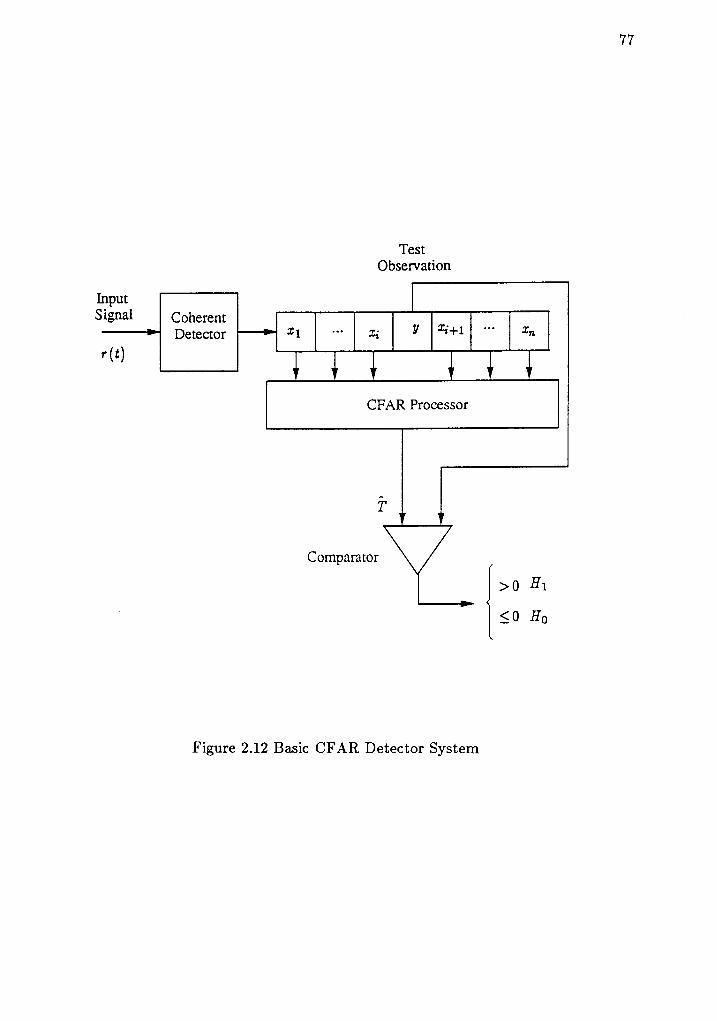
InputSignal

TestObservation

Comoarator

Figure 2.12 Basic CFAR Detector System

[ ' o{| < 0t -

H1

H6

78

adjacent cells are mostly clutter especially when a large number of cells are

averaged. For the instance where cells containing target information axe

introduced into the threshold mean value, the bias is assumed positive (for

stochastically larger distributions under the alternative hypothesis) *d will

decrease the probability of false alarm. Thus, this detector will be able to satisfy

the CFAR requirement for the homogeneous (Chapter I ) and nonhomogeneoru;

clutter observations. Inherently, the probability of detection will suffer from this

contamination. It can be intuitively seen that if the number of auxiliary cells

approaches infinity, then the detector performance is asymptotically optimal.

Thus, there is a CFAR loss (referring to probability of detection) always

associated with this cell averaging (CA) CFAR detector for finite number of

averaged cells.

The extensions of the CA-CFAR detector have been analyzed for different

target and clutter distributions. The work of Hansen and Ward investigated the

CFAR detectors for stationary Gaussian noise using log and square law receivers

to retrieve amplitude information [Han72]. They basically showed that it required

approximately 65% more samples for the log detector to achieve the sarne

probability of false alarm level. The Rayleigh-Rice and Chi distributed models

were investigated for the CFAR detector by Mitchell and Walker [Mit71]. CFAR

detectors for Weibull and lognormal distributions were also examined [Gol73l; "ttd

simulated and asymptotic analysis for the F-distribution and generalized garnma

distributed target models were also applied to CFAR detectors [Nit78]. Basically,

these results illustrate the CFAR loss associated with a given size a for different

fluctuating target models. The next trend of research introduced censoring

contaminated samples containing target information so a.s to lower the CFAR loss

of the detector.

With the advent of censored clutter threshold estimates studied by several

researchers [Han73,Tru78,Wei8Z], the use of partial sums of leading and lagging

cells shown in Figure 2.14 was shown to give more robust detection for the case of

multiple targets. The minima and maxima of the partial sums had different

79

InputSignal

TestObservation

Comparator

Figure 2.13 CA-CFAR Detector System

{l/

> 0 H 1

(0 r?o

80

performance tradeoffs which were studied for the ca.se of exponentially distributed

clutter and Swerling ca.se I (slowly fluctuating targets). The "greatest of' (GO or

maximum) CFAR detector was shown proficient at maintaining the probability of

false alarm under sharp clutter power transitions, but it was also susceptible to

probability of detection loss in the case of multiple targets in the observation

window. The "smallest of" (SO or minimum) CFAR detector was shown to have

higher resolution for discriminating closely spaced targets, but the probability of

false alarm would increase under sharp clutter power transitions.

Rohling [Roh83] introduced the idea of using a single order statistic for the

purpose of robust CFAR detection as is depicted in Figure 2.L5. Assuming

exponentially distributed clutter, he derived an expression for designing the size of

the detector a. In optimizing the rank, he looked at the Average Detection

Threshold (ADT), the expected value of the threshold estimate from homogeneous

clutter observations, and chose the rank with the minimum ADT. Error analysis

of the performance was conducted against several profiles of clutter transitions

with target(s) present under different ranks of order statistics. In this

investigation, the results of Rohling are generalized for several classes of

distributions applied to CFAR detectors and a detailed analysis of the estimators

statistics (efficiency and bias) is given along with analysis of the probability of

detection for several target and clutter models.

Past extensions of Rohling's work include: applications of the trimmed-mean

(censored averages using order statistics [Dav81,Won87]) by Gandi [Gan88] and

Blake [Bla88]; and the function of two order statistics for CFAR detection in

Weibull-distributed clutter. The work of Gandi was confined to exponential

distributions for the clutter and target following Lehmann's alternative hypothesis.

Basically, the study analyzed the trimmed-mean filter in terms of the ADT and

probability of detection for Lehmann's alternative hypothesis. The results showed

that some improvement could be obtained if the trimmed-mean filter parameters

were judiciously chosen.

8 1

TestObservation

lnputSignal

ScalingFactor

Comparator

I f 'o E1- 1 < o E nt -

Figure 2.14 GO & SO-CFAR Detector System

82

Test Sa^mpie Comparator

Figure 2.15 General OS-CFAR Detector Svstem

( r 0 n ' ,1 1 < o r / n

t -

Null Obsenrations

T ( r i r 1 ,

OrderStatisticProcessor

83

The OS-CFAR detector of Figure 2.15 will be analyzed in this research with

the emphasis on the statistical properties of the threshold estimate, i. The

trimmed-mean threshold estimate is a simplified approximation of the censored

ML estimator for the exponential distribution. The r:se of the censored ML

estimator will provide an unbiased a^nd efficient estimate of the scale pa,rameter.

However, the degree of trimming and scaling of the samples will have a.n effect on

the bias and efficiency of the estimate. Thus, the censored ML estimate is

evaluated using Weibull-distributed clutter and is applied to CFAR detection

where the robustness of the detector is analyzed for several target models. An

alternative to the censored ML estimator, is the Best Linear Unbiased (BLU)

estimate which uses order statistics applied to the scaling factor of Weibull

distributions [Dye73]. The BLU estimate is attractive because it is linear and can

be readily updated in terms of a priori information of the clutter distribution,

although the determination of the scaling factors of the BLU estimate may be

more involved. The effectiveness and robustness of these types of estimators are

compared in Chapter III.

The focus is on estimating the scaling parameter for the distribution in the

most efficient manner. For the detector described by Weber and Haykin [Web85],

the shape and scale parameter are estimated simultaneously. No performance

analyses are included on the statistics of the threshold or the robust performance

of this twoparameter OS-CFAR detector. In this research, it is the goal to

investigate how effective this procedure is in comparison with other previously

mentioned CFAR detectors for the case where the skewness of the distribution is

unknown and/or varying.

The following chapter analyzes the design of the discussed CFAR processors in

the context of maintaining the probability of false alarm and examining the bias

and variance associated with each threshold estimate.

84

CHAPTER III

NONPARAMETRIC ANALYSIS OF OS-CFAR DETECTORS

The main goal of this chapter is to analyze different os-cFAR detectors interms of the CFAR design procedure corresponding to different assumptions uponthe clutter distribution. The clutter is a.ssumed to follow weibull distribution inwhich the parameters of the distribution may be partially or completely unknown.The detector considered must be designed independent of the unknownparameter(s) to maintain CFAR performance. In this chapter, several SFARdesign procedures are given which take a robust estimator (e.g., consisting of func-tions of order statistics) of parameter(s) of the clutter distribution and thenmodify it in a nonparametric manner to obtain the required threshold. The dif-ferent CFAR detectors considered in this chapter are briefly described below:

' unmodified order statistic (uos) crAR Detector - uses a single unmodifiedorder statistic to estimate the threshold for any continuous clutter distributionfunction.

' scaled order statistic (sos) CFAR Detector - uses a scaled order statistic asthe threshold for a continuous clutter distribution function with an unknownscale parameter.

' one Paramslsl order statistic (oPos) CFAR Detector - uses a function of asingle order statistic to estimate the threshold that is applicable to certain dis-tributions with one unknown parameter (including the scare parameter).

' Multiple Paramgfsl order statistic (MPos) CFAR Detector - uses a functionof ;r order statistics to estimate the threshold that is applicable to certain con-tinuous clutter distributions with 7 unknown parameters.

' weibull TweParameter order statistic (wTpos) CFAR Detector - uses theaforementioned MPos-cFAR detector results applied to the weibull clutterdistribution with two unknown parameters (e.g., scale and shape).

85

. Censored Maximum Likelihood (CMt) CFAB Detector - uses a threshold esti-

mate comprised of a function of several order statistics that is a scaled version

of the the censored (one-sided) murimum-likelihood estimate of the scale

parameter for the Weibull clutter distribution.

o Tt'irnrned-Mean (TM) CFAR Detector - threshold is given by a scaled cen-

sored (twosided) mean or average value of the clutter observations applied to

the exponential clutter distribution with unknown scale parameter.

. Best Linear Unbiased (BtU) Estimate CFAB Detector - threshold estimate is

given by a scaled version of the BLU estimate (i.e., providing for twosided

censoring) for the scale parameter of an exponential clutter distribution.

The above detectors can be categorized into two groups: (1) uos, sos, oPos,

MPOS, and WTPOS are those detectors with a threshold consisting of a function

of order statistic(s) where an one-toone correspondence exists between the order

statistic(s) (quantile estimates) and the estimated parameter(s) of the clutter dis-

tribution; and (2) CML, TM, and BLU threshold estimators are comprised of

several order statistics which are combined to form a estimate of an unknown

parameter of the clutter distribution. An outline of this chapter follows and the

motivations for using each detector are discussed.

First, the ba.sic OS-CFAR detector will be discussed and shown to be a

distribution-free threshold estimator for any continuous clutter distribution. In this

case the probability of false alarm can be set by r and n alone. This loose applica-

tion of the UOS-CFAR detector is hampered by the fact that large numbers of

processed samples are needed to reach typical CFAR levels (< ro-'). In order to

improve the design flexibility of the UOS-CFAR Detector, a design parameter will

be introduced to give the scaled OS-CFAR detector. The SOS-CFAR detector will

be shown to be nonparametric for a class of clutter distributions with unknown

scale parameters.

The generalized SOS-CFAR detector, the OPOS-CFAR detector, uses a single

order statistic (i.e., quantile estimator) towards the estimation of a pa.rameter of

86

the clutter distribution and modifies it nonparametrically in accordance with the

CFAR constraint. There are applications (e.g., estimated parameters of the

clutter distribution) where the threshold estimate does not satisfy the CFAR

requirement. Thus, there are constraints imposed upon the possible clutter distri-

bution parameters to be estimated and upon the modifying design parameters of

this detector. An academic example will be given for the case where the clutter is

Weibull distributed with and unknown shape parameter.

The multiple parameter estimation procedure will be applied to the MPOS-

CFAR detector which is simply an extension of this one parameter OS-CFAR

detector An application will then be analyzed for the Weibull distribution with

two unknown pararneters including the scaling and shape parameter (i.e., related

to the power and the skewness of the distribution, respectively). CFAR perfor-

mance comparisons will be made for the multiple parameter threshold estimate

OS-CFAR detector and the scaled OS-CFAR detector under va,rious skewed

Weibull clutter distributions. OS-CFAR detector design may be simplified by

using the asymptotic detector design, although the CFAR performance of each

detector will suffer. The degree of this degradation will be examined for the each

CFAR detector.

The second group of OS-CFAR detectors will be then analyzed using multiple

order statistics to estimate the scale parameter of the otherwise known Weibull

distribution (i.e. the shape parameter c is known). First, the censored maximum-

likelihood (CML) estimate of the Weibull distribution will be introduced to allow

for censoring of larger observations (type I censoring) and can be designed non-

parametrically for known shape parameter c. This detector outperforms the other

OS-CFAR detectors considered in this group. If twesided (type I & II) censoring

is required due to the characterization of outliers in the KNS, the Trimmed-Mean

(TM) and Best Linear Unbiased (BLU) estimates can be used in CFAR design.

The BLU estimate is shown to perform better overall than the TM, although, for

large numbers of observations, numerical error is introduced in the evaluation of

the BLU estimate. The asymptotic performance of both detectors is shown to be

87

similar for small censoring suggesting that there are applications for both detectors

depending on the number of processed samples a^nd the homogeneity of the clutter

observations.

The effectiveness (i.e., bias, efficiency, and robustness) of the above threshold

estimators for each OS-CFAR detectors will be examined for the finite and asymp.

totic cases a.s compared to the optimal Bayes detector. Thus, the performance of

these OS-CFAR detectors are evaluated in terms of upon the null hypothesis, and

will be further analyzed in terms of probability of detection in Chapter IV.

Finally, a surnmaxy of the above OS-CFAR detectors will be presented indicating

assets and drawbacks of each system with respect to one another.

3.1 Unmodified OS-CFAR Detector

In this section, the order statistic filter is utilized a.s an estimate of the optimal

one-sample fixed threshold detector. The ideal CFAR threshold, T, is given by the

inverse clutter distribution function /'tl (1-a), where a is the fixed size of the

detector. As shown in previous analysis (Chapter II), the order statistic is a

natural estimate for the inverse distribution function for a given quantile. Thus,

the order statistic can be used to estimate the threshold:

T : r g l (3.1)

where i ir th" threshold estimate given in Figure 1.2. As shown in Chapter II,

this is a consistent threshold estimate implying a.symptotically optimal

performance. In order to determine whether this detector is nonparametric, the

probability of false alarm is found from Equation 1.28:

where

, .@ .

Pr,q,: / o It - rv@)] f;(r) dr

f vQ) : /o (v ) and

(3.2)

(3.3)

(3.4)r;(,): ,(7) rt-' Ol f,- Fo ( r ) l - ' f o@)

under the null hypothesis 116.

and 3.4 into Equation 3.2:

88

Substituting the above expressions of Equations 3.3

u:Fo(r), the above integral can

(3.5)

be evaluated as

, .@

,on: J o

Making the transformation

follows:

,(:) rt-' (") tr - Fok))-'*r 701,1 a,

: '(?) /l: ' ( l ) B( r ,n- r+z) :

(a.oa)

(3.6b)

because it

2.28, the

Ppt u r - r [ 1 - u ] n - r + t O u

n - r * ln * l

where B( ', ') is a Beta function [Abr64]. Thus, Ppa \s distribution-free

is independent of f'o(r). Using the relative rank t of Equation

probability of false alarm is written as:

P r ' c : L - t (3.7)

Thus, the probability of false alarm is determined solely by the relative rank for a

given n. It is important to note that the probability of false alarm also determines

the amount of censoring that is allowed for a given n.

So far it has been shown that the OS-CFAR detector using an adaptive

threshold estimate is distribution-free. However, to understand why the detector

performs distribution-free consider the following alternative derivation of Py.

Since this threshold estimate is changing with each new clutter observatiot, PFA

for each threshold observation c(r) is not a deterministic quantity and can be

thought of as a random variable, denoted as Pra. To interpret this new found

random variable one can think of it as the probability of false alarm which would

result from choosing a threshold from a set of independently acquired order

statistics that remains fixed over subsequent homogeneous stationary test

observations. This random variable associated with a probability is a queer notion

since it assumes that only one threshold observation determines the threshold.

This does not follow the CFAR implementation of Figure 2.L2,b:ut it will facilitate

89

the following argument.

After that rewarding clarification, Equation 3.3 can be rewritten in the form of

input clutter distribution, Fo('), giving the following:

P pt -- f - f'o(Xf ,.t) (3.8)

where the probability of false alarm stemming from one observation, P FA, for this

detector is expressed as a transformation of the random variable of the rth order

statistic, X1r;. From the probability integral transformation (Theorem 2.1), it was

shown that .Fs (Xfrl) is the rth order statistic from a set of random observations

which are uniformly distributed over the region [0,1]. Intuitively and from

Equation 3.8, the expected value of P g with respect to the random variable X1r;

will result in the actual probability of false alarm, Pp1. Let U: l-Fo (X1ry),

Corollary 2.3 shows that U has a Beta probability density function given by:

pu (u ) :nl.

( l - u l | ' - r u " - ' f o r o < u ( l (3.e)( ' - t ) ! ( n - r ) !

where r and n are constants corresponding to the rank and number of

observations, respectively. Through the above equation, the moments and general

statistics of U can be evaluated without any knowledge of f'6 (r). Thus, the

statistics of P p.t (including the mean) are independent of the underlying

distribution, Io (r), and are determined solely by r and n, as in the previous

results of Equation 3.6.

The Ppl of the UOS-CFAR detector is determined by Equation 3.6 governed

by the rank r and the number of observation n where larger values of either r or n

will reduce the probability of false alarm. This can be seen in Figure 3.1 for

n:5,25,and125, where Pp,a is plotted against the relative rank t. The graphs of

Pptr arc linear with respect to I where, for increasing n, the Pp,a decreases for

higher ranks and increases for lower ranks.

The maximum rank shows the lowest probability of false alarm which makes it

the most optimal order statistic in terms of achieving a given Pr,s, with the

minimum number of samples n. From Equation 3.6, the lowest probability of false

90

C)rn

f r .

k

1

0.9

0.8

0.7

0.6

0.5

0.4

0.3

0.2

0.1

00 0.2 0.4 0.6 0.8

Normalized Rank, (r-1)/(n-1)

Figure 3.7 Ppa of UOS-CFAR for several n

91

alarm that can be obtained for a given n ts Lf n*1. For example, if Ppr:6.661,

then the minimum number of null observations needed would be 999. This

requirement may be unrealistic due to availability of homogeneous clutter

observations (further discussion is provided in Chapter V). Other OS-CFAR

detectors introduced later in this chapter will be less restrictive upon the choices

of r and n.

3.1.1 Asymptotic UOS-CFAR Detector Performance. The improvements

that can be gained through increasing the number of processed samples n ca^n be

seen through the asymptotic analysis of the OS-CFAR detector. The a.symptotic

properties of the Ppa can be inferred from results of Chapter II where it was

shown that the order statistic is a consistent quantile estimator. Using Equation

3.8, the asymptotic estimate of Pp1 made while holding the relative rank, t,

constant can be determined by replacing rk\ with its asymptotic quantile

estimate, tr'tt (t),

JgP" , - 1 - r ( ro t ( r ) ) : r - t (3.10)

This result can also be obtained by taking the limit as /D--+oo of .O[fpa] in

Equation 3.8 while holding f constant.

Besides the asymptotic consistency of this detector, the efficiency and the

other statistics of the threshold estimate are indicators of effective estimation and

intuitively support improved detection. Preliminary conclusions made in Chapter I

noted that the higher order statistics show the greatest variances and bias for

Rayleigh and exponential clutter distributions. Thus, the lower the probability of

false alarm of the detector is set, the worse the performance of the estimator will

be and consequently the probability of detection is degraded as will be addressed

in Chapter fV. Since the rank of this detector is fixed by Ppt through the

relative rank, any further reduction in the variance can only be made in terms of

increasing the number of processed samples n.

Thus, the fruits of Chapter II will not be ripe enough to pick until the OS-

CFAR detector is free to choose between several order statistics which can

92

maintain the same CFAR performance for a given n. In the next section, a

scaled OS-CFAR detector will be analyzed in which the order statistic output (the

threshold estimate) is scaled to maintain a given a performance criterion almost

independent of the selection of ranks r and the number of processed samples n.

3.2 Scaled OS-CFAR Detector

The scaled OS-CFAR detector can be seen in Figure 1.2, where the threshold

estimate, ? is given by:

T ( r 6 1 t n ( z ) t ' ' ' r 1 o ; ) - o r e ) (3 .11 )

where the value a is a fixed positive constant. In this section, the scaled OS

CFAR detector is derived for the general case, and is shown to perform

nonparametrically. The optimization of the scaled OS-CFAR detector is done for

Weibull-distributed clutter and the statistical properties of the threshold estimate

are analyzed.

The probability of false alarm can be determined from the threshold estimate of

Equation 3.11:

Pp.a, : PIY > "x olPr,q, : PIY-cX1, ; >o]

(e.rza)

(3.12b)

The value of a can be used to scale the observation up which would produce a

lower probability of false alarm or to scale down the observation resulting in

higher probability of false alarm. For example, if a low ranked observation wa.s

used as the threshold with a:!, the Pp1 would be very poor no matter how

many samples are added, since the asymptotic bound of. Ppl is 1 - f, as wa.s shown

in the last section. But if the low ranked order statistic were scaled properly, it

could produce sufficiently low probability of false alarm. Thus, this scaling factor

allows looser optimization constraints on r and n in this type of CFAR analysis.

From a derivation, similar to the derivation of Equations 1.2U1.25, the

probability of false alarm for this detector can be written as:

93

PFA : /l tt - rv?)l. l h{,to) o, (3.13)

Substituting for ft(') and Fv() from Equations 3.3 and 3.4 and translating the

following integrals by €: rf a and r: f o(f),

pFA: , ( : ) / l t t - r o ( " ) l r f l ( r l a ) [ r - r o? lo ) ] " - ' - + r sb la )d r ( s .ua )

pFA: ' (9 / I t r -Fo(o€) l r5- ' ( { ) [1- ro(€) ] ' - ' foo)a€

PFA : ,g I, ft - Fp(a^Fs-r (r))] u'-t lt- ul"-' du

(3.14b)

(a.tnc)

From the above equation it can be seen that the probability of false alarm is

related to the distribution function .t'o (r) through the expression

[f -fo(aftttrl)]. In order for the detector to be CFAR, the above expression

for Ppl must be independent of the parameters associated with tr'o(r). Using this

constraint, the assumptions of .F'6(z) can be found.

The assumptions of F6(z) needed to make this detector nonparametric and

CFAR, lie in the determination of the scaling factor, o. If this detector is to be

designed nonparametric, then a must also be chosen nonpariilnetrically. This can

be made clearer by examining the asymptotic case illustrated in Figure 3.2, where

the optimal (asymptotic) threshold corresponding to an inverse distribution

function, tr'tt (r), is shown against the relative rank f, where improvement in the

probability of false alarm is accomplished through the translation of relative ranks.

This translation from the chosen rank of the detector, t, to a larger (o> 1)

effective rank l' of the threshold, oF;L (t), must also be nonpaxarnetric. For this

to be true, the optimal value of o must be dependent only on t and t' implying

that

r t t (r ' )o:f f i (3 '15)

is independent of the parameters of f-t (r). Thus, there can be only one

94

r- t (u)

c F - t ( t )

r - t ( r )

Figure 3.2 Graphic Translation of Scaled CFAR Threshold

95

unknown parameter associated with F6l (u) and it must be a homogeneour; factor

of s in the distribution ,t'o("). In other words, there exists a translation y:sf p

whereby the distribution for y, FAfu), is given by

Fo@) : Fo1tv) (3.16)

and is nonparametric in the sense that the pa.rameter p of the distribution is

normalized.

Pplin Equation 3.14c can now be shown to be nonpararnetric under the above

assumption by substituting F;r (u1:rfo t (u) and F6(pz):F a@):

pFA : ,O I l t t - F6@F6L(,)) l , '* ' [r - , ] ' - ' du (3.17)

The determination of Pps is dependent on the choice of r, n, and o under the

assumption of F6(z). Note that the value of ofor finite n is not equivalent to the

optimal value of Equation 3.17 since the sort function will allow neighboring values

of I in the expression [t - F6@F6ttrt)] to influence the result of Ppa.

So far, the problem of estimation of the threshold has been reduced to

parametric estimation of the scaling factor p. This can be seen by considering the

optimal threshold,

T : p f 6 r Q - a ) ( 3 . 1 8 )

Since p is unknown, the above quantile of order l-a is estimated using an order

statistic for the required size a of the detector. The resulting estimate for p, fu is

then given by:

^ r( i )

u : ,-rt 1*s

where u; is the relative rank of rth order statistic, r1,y. The threshold estimate, i,

is found using the estimate ! as follows:

(3.1e)

96

(3.20a)

(3.20b)

where the asymptotically optimal choice for o i" ftt (t-Qlf ;r(u) whereas for

finite r and n the choice of o is given by Fit g-�t'FA) lF 6r fu;) where .Fp1

represents the effective probability of false alarm of the detector which will give

Pp41 a. This effective probability of false alarm is determined indirectly by

solving for o in Equation 3.17 which takes into account the bias and variance

associated with the estimate p. Thus, it will be used to illustrate the relative

CFAR performance of different ranks.

At this point, the choice of rank and number of observations becomes unclear

since almost any scaling factor (within limits) will set the probability of false alarm

to any needed value. Of course for the asymptotic ca.ses the extreme order

statistics are unsatisfactory since they converge to the endpoints of the

distribution so that the threshold converges to zero or infinity. For the

optimization of probability of false alarm it will be shown that several choices of

ranks will satisfy the CFAR requirement upon the proper selection of o.

Although, the bias and variance of the estimate p will have a significant effect on

the probability of detection performance of the detector (the probability of

detection is analyzed in Chapter tV) as well. The parameter o gives us the means

to set Pr.q,. The above relationship may be quite complicated. But in the

particular case where the clutter is Weibull distributed with known shape

parameter, a closed-form solution for Pp1 is obtainable. Thus, the remainder of

this section will explore how the scaling factor a may be determined simply and

effectively for the Weibull clutter distribution.

Given the Weibull distributed clutter introduced in Chapter I, its distribution

function and its inverse can be written a^s:

f o ( r ) - t - " - f u l r ' ) " f o r c > 0

r o t ( " ) : p [ - t n ( r - � u ) ] t ' ' f o r o ( u ( 1

97

(3.2r)

(3.22)

For c:1the distribution is exponential and for c:2 the distribution is Rayleigh.

The normalized distribution F 6@) is evaluated from the above equations for

rr:L. substituting the two above equations into Equation 3.14c, pp1 for the

Weibull distributed clutter ,F'6 (r) is

Prn : '(i) (1 - r )n- ' u ' - r du (3.28a)

PFA: , ( : )B( r ,n - r+a '+r ) (3 .28b)

where B(',') is a Beta function [Abr6a]. The above expression for the probability

of false alarm can be written in terms of the ratio of two beta functions:

r (n+1)

/ , r t - u)o"

P F A :

P F A :

. I ( r ) I ( n - r + o ' + 1 ) . I ( c ' + t )

I ( n+o '+ t ) f (o '+r )

B ( n - r + 1 , a ' + 1 )

where I(') is a Gamma function [Abr6a]. If o'is an integer, then the above

equation can be written as:

P F A :n ! ( n - r + o ' ) !

(n - ra ' ) l (n - r ) l(3.25a)

r (n - r+ t ) I ( r )

B (n+ t , a '+ t )

(t.zta)

(3.24b)

(3.25b)

It can be seen from this equation how increasing a r, r, or n will reduce the

probability of false alarm. The Pp1 for n:2s and a' - 1,5, 10 is shown in Figure

3.3 for the various ranks r:1, "' ,25. For a:1, the p,r1_is linear a.s wa.s shown

in Equation 3.6b. As o is increased the Ppl is reduced considerably for the higher

ranks. In Figure 3.4, a plot of Pp1 is shown where a:5 and c:1.0, l .5and2

corresponding to the exponential, Weibull, and Rayleigh distributions,

respectively, where smaller values of c are needed to maintain the probability of

r-L ( ')

P F ' : I I l - + l; = 0 l n + a " - t )

98

()q)q)

f r

QI(t)

a)(J

a

( r .

1tr

10-1

10'2

10-3

104

L0-5

10-6

10-7

10-8

10-e

Rank

Figure 3.3 Ppl of SOS-CFAR Detector with Various Scaling

99

rnt l

(Jc)c)

f r

OI(n

oq)

(J(t)

106

1tr

L00

10-3

10-6

10-e

1,0'12

10-1s

(c :1 .

0

Rank

Figure 3.4 Ppl o f SOS-CFAR Detector for c :1. 1 .5,2

Weibul

100

false alarm than in the exponential case (c:1). This is importa.nt in some

instances where the. shape parameter of the distribution is unknown, and the

distribution can be assumed exponential so as to satisfy Pr,q ( a for any value of

c ) 1. However, the probability of detection performance will suffer as a result as

is illustrated in Chapter IV. The above examples illustrate that a low Ppy ca^n be

obtained from limited amount of processed samples.

When setting PFA : a, the choice of r and n is not easily evaluated directly

from the above equation and a general solution may be obtained by using

numerical techniques. Newton-Ralphson's iterative technique can be used to solve

Equation 3.25a if the beta function is a sufficiently monotonically increasing

function of a for o ) I to provide guaranteed convergence [Dah7a]. The algorithm

is based on the evaluation of a function of a, f (a), and its derivative to determine

an iterative solution of f (a):0, a^s follows [Dah7a]:

fb;-)a i : a i - r -

I \ r _ )(3.26)

where o; is the present estimate and o;-1 is the previous estimate in which an

initial o6 is chosen and the iterations are terminated when a given tolerance,

lf(oi) l f ' (o;-t) | <e, is satisf ied. The function /(o) can be derived by taking

the natural logarithm of both sides of Equation 3.25a and equating the right hand

side (RHS) to zero:

f (o) :r" f =45t1 , I * r"1r1, -r*a+l)l - h[r(n+o+r)] g.zl)lPror (n- r+t ) j

Taking the first derivative of the above function:

f ' (o ) : V(n- r+o) - V(n+o+1) (3.28)

where !Ir(') is the digamma function [AbrO ]. The choice of o1y will determine

how fast the algorithm will converge, but in general, os ma/ be set to unity. A

better initial estimate of a utilizing the asymptotic behaviour of Ppa is described

in the following section.

101

The required scaling factor at to accommodate a given size a is shown in

Figures 3.5a and b for various relative ranks. The scaling that is required for

a:0.001 is shown in Figure 3.5a, where the lower ranks require much larger

scaling factors than the higher ranks. It is important to note that the scaling

factor will increase the bias and variance of each order statistic differently. As the

number of processed samples increases, the scaling decreases for all ranks. This is

a direct result of the converging quantile estimates for increasing n. For lower

probability of false alarm, a:10-6, the results are similar except that the scaling

factors are much larger and the relative difference between the scaling factors of

different ranks is small. Next, the asymptotic value of the scaling factor is

obtained and comparisons are made to the performance design using the simpler

asymptotic results.

3.2.1 Asymptotic Analysis of SOS-CFAR Detector. The expression for Pp1

may be simplified considerably by examining its asymptotic values. The

asymptotic bound for the probability of false alarm, Pla, is found in general by

taking the limit as n approarhes infinity while holding relative rank t of Equation

3.14c constant and using the results of Chapter II, Theorem 2.1:

lim Pru

Pr.q a rl'1t71)

: / ; / ,

: t - F o (

f o(o F i ' ( r ) + €) 6(u - t ) du d( (3.2ea)

(3.2eb)

(3.30a)

(3.30b)

(s.soc)

The asymptotic value of the probability of false alarm can be determined by

substituting f;' (t): p F;' (t) into the above equation:

Pie :1 - Fo 1o p r j ' ( t ) )- 1 - F o ( o F ; ' ( t ) )

pi,s, -- | - F o1 c "r;r (t) )

where F O() is a known normalized distribution and o *

i. th" asymptotic value of

o. In many instances, the above equation must be evaluated numerically due to

the complex form of the distribution function or in cases where the inverse

distribution function mav not be analvticalh' expressible.

LOz

PFA=0.001

Relative Ranlq t=r(n+ 1)

1018

0.2 0.4 0.6 0.8

Relative Rank, t=r/(n+ 1)

t 1 0ruq)

4 1 0t r

(Jcno 1 s

t t voI)

? 1olcn

(u)

k

I 1nrs

a)r\

d 1012r r

O6

/h\ o 10eL^k

t 1 f f( r

ooa

? 1 F(.)(,

1fl

PFA=0.000001

Figure 3.5 Scaling factor cc of SOS-CF.A.R Detector for given n

103

The asymptotic value of Ppl for the Weibull distributed clutter with known shape

parameter can be described in terms of parameters o *

and t which will describe

general properties of this detector. The Weibull clutter distribution function and

its inverse are given by Equations 3.21a and b. The underlying distribution F a@)

for this distribution is found by setting p:I. Substituting into Equation 3.30c,

the asymptotic estimate for Prt, Pie, for the Weibull distributed clutter is given

bv:

Pie : L - F o(o - J-t t (r- t l l t / ' )

P ie : [ e ln ( r - r )14 ' "

P i e : ( r - 1 1 o ' "

It can be seen from Equation 3.31c that the choice of o *

must be greater than one

to reduce the Ppl and less than one to increa.se it. The reduction is done in an

exponential manner which is attractive since relatively small values of o *

will

reduce Pp1 substantially. The asymptotic analysis of Ppl indicates an alternative

method for selecting an approximate scaling factor for o rather than solving for

the exact value in Equation 3.24 which must generally be done numerically. The

former method of selecting c requires only the evaluation of the distribution

function and its inverse (Equation 3.21 and 3.22). The question is: how close does

the CFAR detector operate to the asymptotically optimal value for finite n?

An example of CFAR performance is given in Figure 3.6a where the

probability of false alarm is given for or for a:0.001 and n:25. The

performance of the CFAR detector designed with a *

shows significant increase for

the probability of false alarm where the marimum order statistic gives the best

performance which degrades significantly for lower ranks. The difference between

the actual scaling factor and o *

.un be seen in Figure 3.6b where the differences

coincide with the detectors' performance shown in Figure 3.6a. It is important to

point out that even small differences in the scaling factor for higher ranks will

produce large degradation in the detector's performance. One reason for this is

that for higher ranks the bias and variance contribute more towards reducing the

(s.sra)

(3.31b)

(3.3lc)

104

(.)

Rank, r

(b)

Rank r

Figure 3.6 (a) Pp.q, Performance of SOS-CFAR with Ideal Scaling,and (b) Asymptotic (Ideal) and Actual Scaling Factor a fora :0 .001

E 1o-1{)()

!\ t0'2U)

ri L0'3

3 tor{)

!r 1trU)

: w

ho

€ 101a(/)

itr

25z010

PFA=0.001

PFA=0.001

105

detector's performance, ali was shown in Chapter I & II. However, the scaling

magnifies the bias and variance of each order statistic differently for a given

relative rank (to achieve a given CFAR size). This effect can be analyzed for large

sample cases by the asymptotic efficiency of the threshold estimate.

The asymptotic efficiency of the estimates is found by using the asymptotic

normal property of order statistics (Equation 2.36) and the corresponding

asymptotic scaling factors, o* (Equation 3.33c). The asymptotic variance,

,orr{i1, of the scaled OS-CFAR detector is then given by:

ro'(r-r"r; ,

' r ( 1 - r ) f o r o < t < 1 ( 3 . 3 2 )rtt (r) /o(ro'(t))

Figure 3.7 shows the normalized asymptotic variance of the threshold estimate,

@lp')'var{i1, fo. Weibull-distributed clutter using Equation 3.21 and Equation

3.22 for various relative ranks, 0 < , < 1.

The relative rank with minimum asymptotic variance can be determined by

setting the first derivative of the above equation to zero for Weibull clutter which

gives:

t + e - 1 (3.33)

Note that this equation is independent of the shape parameter c, thus, solving the

above equation results in I :0.79681213 which is the optimal relative rank for all

Weibull-distributed clutter. This minimum is in agreement with Figure 3.7 in

which the variance increases sharply for smaller ranks. The loss in efficiency for

smaller ranks is of importance since a primary motive for using order statistics is

to provide robust estimates through censoring. Thus, if further censoring of upper

ranks (beyond 2O%) is required, significant deterioration in the detectors'

performance can be expected. Next, finite statistics of the threshold are examined

in order to will gage the validity of the asymptotic analysis.

3.2.2 Statistical Properties of SOS-CFAR Threshold. The statistical

properties of the threshold estimate are analyzed in this section to indicate how

close the detector is operating relative to the optimal detector. Basically, the

,o r r { i } : !n

106

100

90

'o]

, l*l'olool,of2ol

'ofoj

oo

ro

oa)

FO

.t)

N

SOS-CFAR DetectorWeibull-Distribute d Clutter

PFA:0.001

0.4 0.6

Relative Rank, t

Asymptotic Threshold Variance for SOS-

/

0.2

Figure 3.7 NormalizedCFAR Detector

107

normalized mean and variance of the threshold estimates are examined under

various Weibull clutter distributions in which the most effective ranks can be

determined.

The moments of the order statistics stemming from a Weibull distribution axe

given in closed form by [LieS ]:

n["F, f : r ,^ , . ( : ) t f r *mf ct i t - r l t ( ' ; t ) { " - , * r+r1-(r+^t4 1z.z+)r : 0

The Average Detection Threshold (ADT), i:oz1r; is evaluated a.nd shown in

Figure 3.8 from the above equation (m:1) and Equation 3.26 for the case where

n:25 and the probability of false alarm is set for a:0.001. It can be seen that

the lowest ADT occurs at r:2L corresponding to t:0.80769 which coincides with

the previous asymptotic analysis. Some increa.se in the ADT associated with the

ma><imum rank which is due to the larger error associated with the murimum

order statistic as shown in Figure 2.9 of the normalized MSE of order statistics.

The corresponding variance and MSE of the threshold estimate, o x14, fot

Rayleigh distributed clutter can also be evaluated from the Equations 3.26 and

3.32. The variance and mean square error (normalized with respect to p) u"

shown in Figure 3.9a and b, respectively, for c:1, 1.5,and2 and n-2s. These

results follow the ADT and also confirm the previous results.

3.3 Generalized OS-CFAR Detectors

In the previous section the scaled OS-CFAR detector was shown to be a con-

sistent estimator of the scale parameters for any continuous clutter distribution.

In this section, the OS-CFAR detector is generalized for the estimation of the

other clutter distribution parameter(s) considered. An example of this is given for

a class of Weibull distributions for which only the shape parameter is varied and

the threshold estimate is derived. Basically, the order statistic can be used to esti-

mate any parameter of a distribution so long as it can be written as a function of

quantile estimates. This does not, however, guarantee that the detector will per-

108

c:2.0

Figure 3.8 NormalizedDistr ibutions

ML Normalized ADT

Actual Threshold

PFA:0.001

c :1 .0

c= 1.5

Rank, r

ADT of SOS-CFAR Detector for Weibul l

aoa)

f r

UI(h

(t)

d

F.

q.)N

E

z

109

1 0

9

8

7

6

5

4

J

2

I

00

10

9

8

7

6

5

4

2

1

00

Figure 3.9 Normalized (")Detector

Rank, r

ML Normalized MSEPFA:0.001

Rank, r

Variance and (b) MSE of SOS-CFAR

!AI

oq)Lr

-ti

il

4a r

U,ht'\a

/ \ q

ia l oc)(Jtrkd

a.,N

dF

|<A

>2A

EA

oc)r<F-

F{f | .

r lv

Iu)a1

rb) 6\ - /

kA

r Y l

v)

d

0)N

FkA

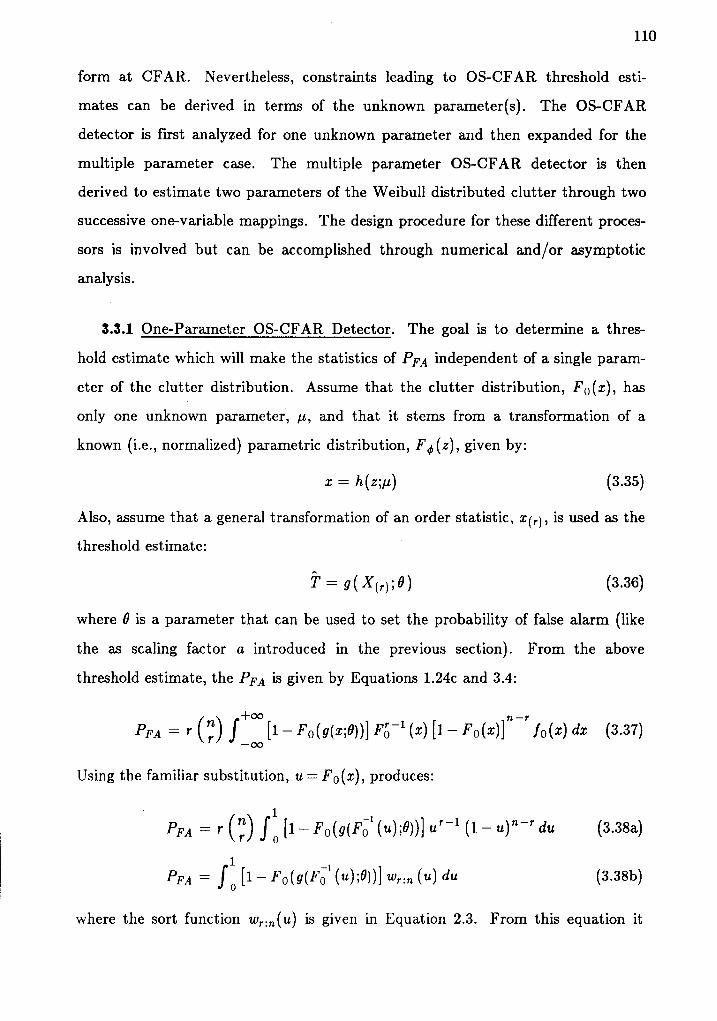
110

form at CFAR. Nevertheless, constraints leading to OS-CFAR threshold esti-

mates can be derived in terms of the unknown parameter(s). The OS-CFAR

detector is first analyzed for one unknown parameter and then expanded for the

multiple parameter case. The multiple parameter OS-CFAR detector is then

derived to estimate two parameters of the Weibull distributed clutter through two

successive one-variable mappings. The design procedure for these different proces-

sors is involved but can be accomplished through numerical and/or asymptotic

analysis.

3.3.1 One-Parameter OS-CFAR Detector. The goal is to determine a thres-

hold estimate which will make the statistics of Pp,a independent of a single param-

eter of the clutter distribution. Assume that the clutter distribution, Fo(z), has

only one unknown parameter', p,, arrd that it stems from a transformation of a

known (i.e., normalized) parametric distribution, F6(z), given by:

x : h ( z ; p ) (3.35)

Also, assume that a general transformation of an order statistic, r1ry, is used as the

threshold estimate:

T : g ( X g y ; 0 ) (3.36)

where d is a parameter that can be used to set the probability of false alarm (like

the as scaling factor o introduced in the previous section). From the above

threshold estimate, the Pp1 is given by Equations L.24c and 3.4:

/ - \ n - f @ , , - . r , . r f t - lpFA : , l:) /__ [r - ro fu@;q)] r,5-' (") [t - ro1";] -

f 6@) dx (3.37)

Using the familiar substitution, u: Fo(c), produces:

PFt : ' (?) J: t t - ro(g(r0 ' ( , ) ;d)) l u ' - r (1 - u)n- ' du (3.38a)

PFA : / : t t - ro (g( ro ' ( r ) ;d ) ) ] w , .n (u) d ,u (3.38b)

where the sort function wr,r(u) is given in Equation 2.3. From this equation it

1 1 1

can be seen that Pp.t is independent of the parameter p, if the expression

fo(g(tr'ot(r);r)) is a function which can be evaluated by d and u alone over all

allowable values. Using the assumption that the parameter p is governed by the

transformation on the clutter distribution, Fe(r) :FO(h-'(sip)), where h-'(r;tt)

is the inverse transformation, the above expression, Fokgi'{ru)te)), can be

written a.s:

ro(g(ro ' @);0)) : F o@-'@&1rj ' wt ; p) ;0) ; p)

A solution may be obtained if the functions h(r;p) and g(r;d) were commutative

in the above equation since p would fall out in the expression of

n-' \@gj' $l;0); p);p). This solution mav be expressed as:

s (h ( r ; p ) ; 0 ) : h (g (x ; 0 l ; p ) (3.40)

where g(r;0) is given by:

(3.3e)

(3 .41)

(3.42)

with the condition that

s(r ;0) : h(r ;g)

g ( g ( r ; p ) ; 0 ) - - s ( s ( r ; 0 ) ; p )

This is only a simple solution to the problem and is by no means a unique

solution. However, other solutions are as dfficult to find. Many g(r; p) will satisfy

the above CFAR conditions such as scaling, shifting, and exponential functions.

Note that the distribution tr'o(") is assumed continuous and has positive nonzero

values for the all points on the real line [-m,*oo]. If this is not true, then the

above procedure will remain nonparametric only if ,F6(c) can be evaluated

nonparametrically at the endpoints or at the discontinuities. For the one-sided

distributions considered in this research, the shifting property may not be

compatible with the CFAR constraint since the lower endpoint of the integral in

Equation 3.38 cannot be determined nonparametrically.

The Pp1 under the above solution of Equations 3.42-44 on .F6(r) with properly

chosen g(r;0 ) can be written as:

rt2

PFA: ' ( : ) / l f t - � pok (F i '@) ,q ) l u ' - ' ( t - � u )n - ' du (a .+e )

The above expression of Ppl is independent of p yet the determination of d in

order to set PFA:a may be involved. As with the previous exalnple of the

Weibull distribution with known shape parameter, the value of a could be either

calculated by numerically solving Equation 3.24 or approximated with the simpler

asymptotic expression of Ppy for the large samples case. The general asymptotic

analysis is given below to illustrate how these estimates will perform for large

samples and give a general understanding of the small sample design.

3.3.2 Asymptotic Design of the One-Parameter OS-CFAR Detector. The

asymptotic value of the Pro, Pio for n approaching infinity with constant relative

rank t produces the following results:

Pin : r - Fok7 i ' ( t ) ;d - ) ) (3 .44)

where d* corresponds to asymptotic parameter setting. Knowing from Equation

3.41 that functions g and h are equivalent, Equation 3.44 becomes:

pi ,q : r - Fo0@; ' t t t ;or ) ) (3.45)

From this relationship it is apparent that the parameter d* replaces the unknown

parameter p in the clutter distribution F6(z). Thus, asymptotic 0,0* rs found to

meet the required s\ze, Pla: c r for a given relative rank by simplifying Equation

3.45:

h(F; ' ( t ) ;o r ) : F i ' 0 - P io )

and solving for d*. The optimal parametric value for 0, 0r can be used to

approximate 0 for finite r and n. Pfa must, however, be chosen lower or equal to

the effectiu" Fro in order for the detector to perform with Pp1 ( o, a.s was

illustrated in Section 3.2 f.or the example of Weibull distributed clutter with

unknown scale parameter. Again, the choice of rank is not critical for the

asymptotic case, except where l:0 and f :1 in which case the extreme values of

Fi'(t) may be independent of 0 since they converge to the end points of the

(3.46)

113

distribution. When r and n are finite, then 0 must be properly chosen to account

for the bia.s on the threshold estimate as was shown in previous sections.

The bias of the threshold estimate is, of course, a result of the bias of the

parameter estimate d. The parameter estimate 0 can be found by substituting the

quantile estimate, z1r1 in Equation 3.46, producing the following results:

s(,) : n-' @i' @);p) (3.47)

in which i, ^uy be solved in terms of xg,1 ana f/' (ur). The properties of both

functions, h(r) and tr'6(z), determine the bias and varia.nce of the nonparametric

threshold estimate.

3.3.3 Weibull One-Parameter OS-CFAR Detector: Unknown Shape Parameter.

The one parameter OS-CFAR design results can be illustrated in an example

where the clutter has a Weibull distribution:

F o ( r ) - 1 - r - @ l u ) n ' f o r r ) o ( 8 . 4 8 a )

Fo@) - 1 - e - ' u ' f o r r .>o (8 .48b )

and p1 is the unknown shape parameter and the scaling parameter p2 is assumed

normalized (pz : 1). The transformation h (r; p) : tPt dictates from Equation

3.39 the form of the threshold estimate for the OS-CFAR detector:

i : g( rk) ;o) : , [ l (3 .4e)

The asymptotic value of d is found from Equation 3.44 for the above

transformation:,

r - - l r r t O ^ - l r - *

l Fa '@)1" - F6 $ - P re )

Solving for 0r ,

(s.soa)

(3.50b)* ln F6' G - Pie)0 : - r n m -

w h e r e F O @ ) : I - e - ' .

Figure 3.10 shows an example of what values of d can be used to attain a

probability of false alarm rate of 0.001 in the asy'mptotic case. This figure shows

tt4

-100

PFA:0.001

l n n l " '-4\.'\.'o o.z 0.4 0.6 0.8 1

Relative Rank. t

Figure 3.10 Ideal Design Exponent Parameter for CFAR-Detector

50

o

q)

0)

(u

Xr r'l

q.)

-50

-150

115

that the lower ranks need negative values of 0 for the given Pp1, while the higher

ranks, conversely, need positive values. This is intuitive, since the lower ranks

correspond to observed values less than one and the negative exponent d will

increase the threshold values. It is also important to note that all the ranks are

able to satisfy the CFAR requirement asymptotically. Next, the values of. 0 are

investigated for finite r and n.

To see how 0 is chosen for finite r and n, the integral of Equation 3.43 is

determined for F6 ( ' ):

Pp.t "*p(- [ - t t t ( r - r ) ]d ) w, . , (u) du (3.51)

where urr.n is the sort function defined in Equation 2.3. The above integral cannot

be simplified to a closed form expression, and therefore can only be evaluated

numerically. From Figure 3.11 it can be seen that there is a lower limit on the

probability of false alarm that can be obtained for Nry 0 of a given rank. The

lower rank, r:1, shows minimum probability of false alarm (Pp,q,:0.005) for

negative values of 0. There exists a sharp transition at zero where there is an

increase in Ppa for the lower ranks and a decrease for the higher ranks. This is

due in part to the region of observations which are emphasized. For lower ranks

the observations of values less than unity are emphasized, which means that in

order to decrease the probability of false alarm, d must be negative. It is is

important to point out that for each of the ranks, Pp1 has a lower bound.

Thus, depending on how low the required probability of false alarm a is set,

the detector may not be able to perform for some or all the ranks. This point is

illustrated in Figure 3.12, where the values for d needed to set Ppa:0.001 are

shown for the different ranks of an OS processor with n:25. For this example,

ranks 1-5 and 24-25 are the only ranks which will meet the required size a. As

was shown above, the extreme order statistics provide the ability to rearh lower

Pr,q,. Despite this, the extreme ranks are usually not attractive since they are

more susceptible to outliers. Thus, in order to use intermediate ranks, the number

of observations n must be increased.

: / :

116

- 1n- r{ r v

(u4

f r

€ 'to-2

10-3-40 -20 0 20

Exponent Parameter Value

Figure 3.7I Ppl for Exponent Design Parameter

40

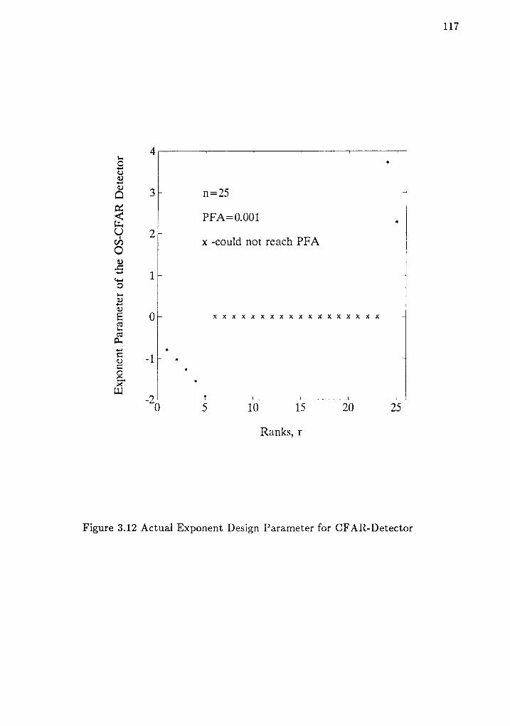
tt7

ac)q)

?O

I

a

q)

Lr

{)

q')

xf T ' l

15

Ranks, r

Figure 3.12 Actual Exponent Design Parameter for CFAR-Detector

n:25

PFA:0.001

x -could not reach PFA

x x x x x x x x x x x x x x x x x x

118

This procedure can be extended to the multiple parameter case if, through

successive translations of F6, Equation 3.42 holds true for each estimated

parameter of the clutter distribution. It can be inferred from this analysis that the

threshold requires one unique order statistic to estimate each parameter and only

one variable parameter 0 to set the probability of false alarm. In some

circumstances, certain order statistics a,re not asymptotically optimal since they

will not converge to the proper size o. Such is the case for the scaled OS-CFAR

detector under an exponential distribution as in Equation 3.50b, where fixed ranks

at r:1 and r:r? are unsuitable since they would correspond b Pla of l and 0,

respectively. Although Pio:0 is attractive, under a simple thresholding it would

mean that the probability of detection would converge to zero as well. This is, of

course, a condition never met for the relative ranks chosen in Chapter II,

t:r l(n*1), since they do not include the endpoints for finite r and n.

3.4 Multiple Parameter OS-CFAR Detectors Design

In order to understand the constraints on the functions h(r) a"nd 9(r), the

expression for Pp1 must be examined as was done for the one parameter case.

Since the threshold is dependent on fr distinct order statistics corresponding to a

distribution containing ft unknown pararneters, the Pp1 is given in terms of the

joint distribution of order statistics:

" f @ " * @p r e : [ . . t I r - r o ( g ( r t , . . . , 2 k ; 0 ) ) ] f o Q t , . . . , , z * ) d z y . . . d z pt - @ t - o o

(3.52)

w h e r e ( , , , . . . , r ) , : ( g ( n , ) . . . r ( n t ) ) ? f o r w h i c h L 1 n 1 ! n z 3 . . . < � � � �

The parameter d is a scalar quantity, since ft-l of the elements in d can be

represented in terms of the order statistics (tt,,..., t*). The 0 notation is used to

facilitate a solution in terms of separate translations for which the derivation of

g(Z;0) is discussed after the constraints of this transformations are derived.

The joint distribution of order statistics 'Dav81l is substituted into Equation

3.52:

119

pFA : " ' / ] : / l : I r - ro (s@t, . . . , zh;o)))

k

.n [ ro( , i * , ) - ro( , , ] l ' l ] ' - " ' - t n n e i )d21 . . .d , r (s .s ' )

i :o (ni+t - nt

i :r

where .Fs(zs) :0 , Fs(zt .+1) :1, z !0:0, and f lk+r :n*L. Using the

tra"nsformation z; : h-'(r;; ttr, ..., p*) the above equation becomes:

pFA : " ' / l : / l : Ir - ro (s@-'(,,), . . . , h-'(,r) ;r))]

+ IFo@i*r) - Fo(w,1]ni+rn ' - tI I / - - r l ri j ,

(n1+t - n1- r) l

The term Fo(gf t - ' ( r r r r ) , . . . , h- ' (w1,) ;0) ) must independent of FLt " ' , p* in

order to fix Pp1 nonparametrically.

A solution can be obtained if functions g and h satisfy the property below:

g(h- ' ( r r ) , . . . , h - ' (u* ) ;0 ) : h - ' ( g@r, . . . , w* ;0 ) ) (3.55)

The solution for g is more complicated and involved for the multiple parameter

case since it can only be derived from the solution of parameter estimates from the

asymptotic analysis. This can be verified by simplifying Equation 3.54 using the

above assumption:

n * @ n * @

Pro -- I I J- r o(s@r, , . . . , wk;o)) lt - o o t - @

il o@i)1n111-ni-r\ lro@ir+r) - Fo@i)

(n1+r - n1 - I ) l f o@) d r r ' ' ' d r r (3 .56 )

independent of the unknown

k

IIj : l

; b e

f 6 @ ) d w t " ' d r r ( 3 . 5 4 )

k

ilj : L

ow

i :o

Thus, the above expression for Pp.q, is n

parameters of .t'6(r).

Knowing the conditions upon g(Z;0) which will make a threshold estimate T

CFAR, the actual simplif ication of g(Z;i l to g(Z;d) must be addressed. Since

the transformation is over two unknown parameters, the composite threshold is

determined by introducing the order statistic estimates in the inverse distribution

L20

function of Equation 1.12. Solving for the a.symptotic casie, a simila,r solution can

be obtained for the parameter d where an effectiv e Ppt, Foo is used in Equation

3.2O to represent the value of the parameter, which would produce the

corresponding Ppa. Then, for each individual transformation, the subsequent

parameter d is replaced by the composite parameter 0, which is a function of .Fpr1

and the asymptotic values of the order statistic quantile estimates. This will

hopefully be made crystal clear by the following example.

3.4.1 TwePa"rameter Weibull OS-CFAR Detector Design. An example of

multiple parameter OS-CFAR detector design is now given for the Weibull

distributed clutter with two unknown parameters, scale and shape. This

distribution is given by:

r o ( " ) - 1 - r - @ l u r ) p ' f o r r ) o (3.57)

where Ltt ffid Fz fre shape and scaling parameters, respectively. The normalized

distribution considered, F4(r), is simply an exponential function e-', although

this derivation is applicable to any known distribution F O@). From the

transformation h(r): -@lp)P' and Equation 3.55, g(r) is given by the

threshold estimate below:

i : g ( r1 l ; ! ) : ( " ( , ) le r )o t (3.58)

were 0 is a vector depicting all translations. Note that the outer exponential

operation is the first translation, then it stems from another order statistic,

(r1r;,s+r). Also, it can be seen that the parameter d2 is dependent on r1a; since

it is irlso dependent on the estimate of LLL. As stated in the previous discussion,

this derivation is slightly more complicated than the more direct method of solving

for one composite parameter. Therefore, the derivation will be based on

s ( r O ) ; ! ) : r 6 1 f 0 2 .

In order to use the second translation, the underlying distribution tr'6 must be

updated to include the estimate of p.1, ir. The estimated parameter !t is found

from Equation 3.57:

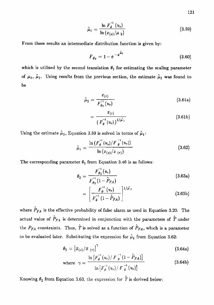
- 1 .

^. _ ln FO (u,)* t -

l r , ( ro l lp r )

From these results an intermediate distribution function is given by:

-itn a ^ - Lr 6 2 : l - Y

f r r : #_

r(r)- r t | i

( F 6 . ( u , ) ) , , n ,

Using the estimate fu2, Equation 3.59 is solved in terms of fia:

h (rJ' @,) I F f' {r,,))

12l

(3.5e)

(3.60)

which is utilized by the second translation 02 for estimating the scaling pa.rameter

of pz, itz. Using results from the previous section, the estimate p2 was found to

be

itt :ln (r1,y l, Ol)

The corresponding parameter 02 from Equation 3.46 is as follows:

riitu,)

(e.ota)

(3.61b)

(3.62)

(s.osa)

(3.63b)

(3.6aa)

(3.64b)

02riO - i'ro)

I ri' fu,) 1't'' ': L" i ( t-F"r l

where i'pa i" the effective probability of false alarm as used in Equation 3.20. The

artual value of Ppa is determined in conjunction with the parameters of ? under

lhe Ppa constraints. Thus, iis solved as a function of Fp1, which is a parameter

to be evaluated later. Substituting the expression for fu1from Equation 3.62:

r,2: lr1,1l, oi'n [r/' (u,) I F J' (r - i'ri]

where 1 -

h [ rJ ' (u . ) / r , ' ( r , ) l

Knowing 02 from Equation 3.63, the expression for i is derived below:

i : 1 6 l 0 z

r +.y - . t | ' , , , I '

: f , (r) ' r( t) : ' , t , L , ,

l

( n 1 + r - n j - l ) t

122

(3.65a)

(3.65b)

where 0 : - 1. It can be seen from the above relationship that 0 is dependent

upon the effective probability of false alarm, Fpy, and, the inverse quantiles of the

underlying distribution F6 (c) for ranks r and s. Following the assumption that

r<s ( i .e., r1r; ("(r)), then larger values of 0 ( i .e., 0>L) wil l produce smaller

thresholds and subsequently smaller probability of false alarm. In meeting a

required probability of false alarm, a, the choice of d is based upon the effective

value of Pp1, which for finite observatiom Fa1 * a, and error (e.g., bias and

va.riance) associated with i which must be taken into consideration.

For the previous example, h(r) and g(r) from Equations 3.57 and 3.58,

respectively, satisfy the property in Equation 3.55 which results in the following

expression for Ppa:

F T @ F w z .Pre, : I I ] - ro( , ! - ' ,o rDlr c - - oo

lF o@ i * r ) - F o@ i ) ln i s - n1-r2

ilSubst i tut ing u -- F A@), u: F d@),

Pp. l , : t (9

. u r - L ( , _ , ) r - r - r d u d u

Simplying by transforming u) : t! /u produces

2

ili : l

, ( ' ; t ) / , , r - u)n-s / ; t t - F o(1rJ ' t , ) )1- ' {F ; ' t , l } ' ) ]

f o @) d w1 d w2 (3.66)

(3.67)

123

PFA : ' (9 / , , t - u)n

-s , ' r - t

' n) '-t ( l - ,) '- ' -t arla"

{ , {";') /, t'- r oeri'(rr)\t-o 1rJ'trl ld)1

(3.68)

From the above relationship it can be recognized that the two integrals are of the

form of OS quantile estimators. The inner and outer integral estimates the

quantiles corresponding to the relative ranks tr: r ls and t s : s l@+t)

respectively.

For the Weibull distributed clutter where F O@): e-x, the Ppl are given by:

Pr . r : ' ( 9 / r , t - u )n -s t ) ' - t r ( ' ; t ) / , f t - r r l n [ l n ( r -u ) / l n (1 - ' q ]0

. r r r - r (1 - , ) r - ' - r dw du (3.6e)

This can not be simplified further and must be evaluated numerically through

multivariate quadrature techniques. Taking arr example where n:25 and 0:2,

the Ppa of the detector is shown in Figure 3.13 for ranks s > r. This reveals that

as the r and s separate, the probability of false alarm decreases. Also note that

higher values of s for sets of ranks with the same separation, s-r, will produce

lower Pp4.

The required scaling needed to achieve a given probability of false alarm

a:0.001 is shown in Figure 3.14. For certain values of r and s the parameter

value became very large for small separation of ranks and these are not included in

this figure. As expected a smaller exponent is needed for ranks separated far

apart while it increases significantly for ranks close together since the ratio

r(r)lr t) is closer to unity. Next, the asymptotic solution of this detector is

derived and compared with actual finite design values of exponent d.

L24

0 : 2 . 0

as ;s

1 ' 5

B.u$o'

Figure 3.L3 PFADetector

for Fixed Design Parameter of WTPOS-CFAR

125

PF.t:0.00r

sh

€

fr

Figure 3.14 Designn :25

Parameter 0 for WTPOS-CFAR Detector for

126

3.4.2 Asymptotic Analysis of WTPOS-CFAR Detector. The asymptotic

value of the expected value of P|,a, Pio is found by taking the limit of Equation

3.7O asi n approaches infinity while holding tr:rl(n+l) and tr:sl(n|L)

consta.nt. fla is then given in general by:

Pie : L - F ({F;' (r, r,)}t 1r/' (t,)}t-d)

The quantity trt, can be written in the asymptotic limit a"s:

lim t, t,, :n + @E+OOf + @

(3.70)

(3.71a)r. ,t r

n+o n *L . 9E + @r--+oo

, . fIlm -

n--+oo n *18-+OOr+@

+ 'v r

(3.71b)

(3 .7 lc)

The above Equations need not have had the limits imposed on them since the

equality holds for any values of r, s, and n. Yet, for other definitions of relative

ranks, t, and t' they might only hold true asymptotically. Equation 3.70 can be

written as:

pi,s, = 1- r({r; ' 1t',1yt-t '{r; '(r,)}d ) G.72)

and for the Weibull distributed clutter where F a: e-", Pit is found through

the above relationship:

- * t , . . , [ l n ( l - t , ) l } n ( t - t ' , ) )eP F A : [ 1 - t ' r ] ' (3.73)

The ideal values of d for a:0.001 are shown in Figure 3.15a. The values of d for

n:25 in Figure 3.14 and d* show small differences, yet small deviations in d can

produce very large degradations in Pp1. Figure 3.15b shows the actual Ppl f.or

n:25 and various ranks where the detector is designed using ideal d* with

a:0.001. It can be seen from this figure that ranks with large separations not

including the extremes produce the Pp.q, close to d. Next the statistics of

threshold are examined to characterize the effectiveness of the estimate in terms of

PFA:0.001

L27

i \ ,

d

\

s

r d E

tr

ad

=_>

Ppt

1 , 9

B.a$t'

Q**, , 3'os\F'

Figure 3.15 (a) Ideal Design Parameter 0' for WTPOS-CFARD,etector and (b) Pp1 of WTPOS-CFAR Detector Designed Using0

L28

the ranks used.

3.4.3 statistics of the wrPos-cFAR Threshold Estimate. The statistics of

the threshold for the two parameter CFAR detector can be evaluated numericallv

from the following:

E[ i^ ] : " ( : ) , ( ' ; t ) / , , t - , ) " - ' I :

' t t ' ' -r (a - u1t- '-r du du

Using Equation 3.22, the moments of i become:

E[ i^ ] : , ( l ) , ( ' ; t ) / l r ' - u )n -s I i r ^

I t"; ' (r)]t-d {ro' trt}'] -

I trJ' (,)]'-' 1r;' @]'l^t'

(3.74)

' t t ' - r (u - v\ t- ' -L du du (3.75)

where F 6: "-'. The moments of the threshold are dependent upon p and c and

will be examined for normalized p, and c : 1 and 2.

The mean and variance of thresholds for various skewed clutter skewnesses are

shown in Figures 3.16 and Figure 3.17 for n:2s. The minimum mean and

variance is associated with the ranks of s near the macimum and the ranks of r

slightly greater than the minimum. Note that for the exponential clutter

distribution in Figure 3.16 (c:1) the minimum mean is 11.91 which is larger than

the ADT of the scaled OS (r:21) at 8.48 (Figure 3.7). This is also true for the

variance where the minimum of Figure 16b is 34.55 and for the Scaled OS

threshold where the minimum of Figure 3.8 is 4.36. Thus, the 2-Parameter is far

more inefficient and can be expected to require more samples in order to perform

equivalent to the robust solution of the scaled os-cFAR detector.

The performance of the detector with Rayleigh-distributed clutter (c:2), the

minimum mean and variance of the 2-Parameter CFAR Detector are 3.3625

(Figure 3.17a) and 0.6053 (Figure 3.17b), respectively. In comparison with the

scaled OS-CFAR detector statistics, where the minimum mean and variance are

L29

(.)

(b)

Figure 3.16 NormalizedDetector for c:1

. h

a

oN

CI

ts{

II/

l< Fr i'. -l! - l

A ] -J

N .r \ l

A ]J

Fr ^- id t - l - l

' 1- l

o t - iN r i : i' ] :

!

Ft ) :

t { " 1 .A - . _ l

2 ll

Irn '1_, -+-.

.-.t: -

Eaarr, ,

8."$o'

(a) ADT and (b) Variance of WTPOS-CFAR

r30

c--2

:\ J

. !

(F\ N -l' v - l. ! " 1O ' t - lF N JA \ {

4 " r J, j :' n * - l

o - lN n - l

d r i - 1d - ' - i

r r * l

Z t r l t' t t

' � s - l l-.-1- '

:l-

€--->

(")

j>-,

:'\

%) -],-..-.

n , ItN

. tti -lt ! f i J

A

Io . l( J \ _ l

l

A I!

! ' r ' 1d , !

(b) rr .\ / o ' lN * - r

q J!

< d ' lH } :H Jk . - t lA t i

t it - _ l i, : - L - - : ' l

':.- r' '- -; j

€-

.alr^'qhL

i :,-! - ' , . -i . - ; - . '

1 r S

&ast'

Figure 3.12 Normari'sfl (a) ADT and (b) variance of wTpos-cFARDetector for c:2

131

2.89 and 0.126, respectively, the efficiency of the 2-Parameter CFAR detector is

better than the scaled OS CFAR detector (c:1) yet shows significant losses for

Weibull-distributed clutter with c:2. The choices of ranks r and I a.re rather

restricted since the performance deteriorates sharply. Thus, if suspect wide

deviations in the shape parameter c exist, and the observations robustly represent

the clutter statistical information, then the use of this detector would be more

attractive. However, significant losses in efficiency arise, a.s was illustrated in the

above example.

Further research is needed in determining a method which would utilize

several order statistics to estimate both the scale and shape parameters in concert.

This problem is involved and has been studied in the past [Men63,Har6ba,Har65b]where the censored-Ml estimator of the two parameters requires iterative

solutions for each set of observations. This feature would require more complex

computations with each observation and corresponding KNS in the design of

CFAR detector which may not be practical for large amounts of data. Thus, in

the remainder of this thesis, the focus is on using multiple order statistics to

estimate only the scale parameter of several clutter distributions.

In the following section, the focus will be on designing the CFAR detector

using multiple observations in a Mucimum Likelihood estimate to improve the

efficiency of the scale parameter and its corresponding threshold estimate.

3.5 Censored Maximum-Likelihood OS-CFAR Detector

The goal of this section is to utilize censored ma<imum-likelihood estimates of

the scale parameter of Weibull clutter distributions and apply them to CFAR

detection. The motivation behind searching for a maximum likelihood estimator

lies in the fact that minimum variance is achieved in the estimate which will

improve the detectors performance as shown in Chapter I. In previous sections,

only one order statistic was utilized as an estimate of the threshold for each

unknown parameter of the clutter distribution and consequently the efficiency of

the estimator suffered. It would be attractive to utilize more information in the set

t32

of n observations of the KNS without introducing error due to outliers (".g.,

target-plus-clutter samples) within the KNS. These samples must be chosen such

that they are less susceptible to the introduction of target information or spurious

noise. In general the outliers are found in the extreme or larger ranked order

statistics. Thus, this section analyzes the design of ML-CFAR detectors which

make use of a selected m smallest observations out of n order statistics. for which

the improvement in efficiency is presented.

Work on censored ML estimates of the scale parameter of Weibull

distributions has been done by Epstein and Sobel [Eps53] in the field of life

testing. The censored data utilized in the estimate were the order statistics

corresponding to r l), re),.. . , r(m) where the upper ranked n-m order statist ics

are not used. The joint density function of these observations for Weibull-

distributed clutter is given from Equations 3.S3 and 3.21:

f * ( r ( r ) , r ( z ) , ' ' ' , r ( ^ ) ) : # [ r - ro ( r r . t ) ] n - ^

^

. f o ( r t i l )i=L(3.76)

f *@G), r14, , r(^)) :#*),| ^ . - l' '"0 | ,!,( ',t t ld ' - @-^) @o ld '

| (3.77)

Making the t ransformat ion, Y; :X( ; ; for i :1 ,2, . . . ,m) the above jo in t

probability density becomes

fr(vrta2, - . . ,u^): # tr-^, expl; ,, -

c - i m c _ � r

r * ) f r r \ i t

i , , , - (n-^)r. I l (3.78)i : r ) l

From this equation it can be seen that the expression, ! ; !_tvi+@_�m)u^, k

the suf f ic ient s tat is t ic o f the jo in t densi t l ' funct ion, t 'v (yr , !2 , . . . ,u^) . That is

to s&y, this expression contains all the information provided by the m

observations.

The maximum likelihood estimate of the scaie parameter, fi,, for the Weibull

distribution of known shape parameter. c. car be derived in a similar fashion to

133

Equation L.41- 1.44, and is found to be [Eps53,Har65]:

^ r ( - ) l ^ c ' \ ci': 1r*;fi | ,I,ril * (n -m)a1^1

r l t

(3.7e)

Note that this is the ML estimate for m-samples where the censored samples do

not contribute information to this estimate. Defining a.n unscaled estimate, D, by

the following:

D : i , T (m+L lc ) l l@) ,

This statistic has a ganrma probability density function [Har65]:

(3.80)

, , c m - l f I

l t@) : " t ^ \#^ " *p l @ld ' )L lm)LL-

" L

where the threshold estimate for the CML-CFAR detector

ML estimate,l:

i : 0 i (3.82a)

(3.82b)

where the design parameter d is chosen to satisfy the CFAR constraint and which

satisfies Equation 3.55 of the previous section.

The probability of false alarm of this ML-CFAR detector is given by Equation

1.24 and 3.81:

(3.81)

is given the unscaled

(3.83a)

(3.83b)

1.47a-|.47c

^ l ^ t " t 1 t l 'r : o L ' '?'"itt

+ (n -^) r@ l

r * - . rPFA : J _"" [t

- ro(")J V f tk l0) dr

pFA:/ l : #"*o [ - 0- ' ) " , lu , la,

This equation can be solved using similar steps taken in Equations

which leads to the following:

P F t : ( I - g ' ' " ' ( 3 . 8 4 )

This expression implies that this method *:.. u:il ize the m samples in exactly the

134

sarne manner as the ML example of Chapter I with only a reduction in sample

size.

3.5.1 Asymptotic Analysis of the CML-CFAR Detector. The a.symptotic

scaling of the threshold estimate can be seen from Chapter I (Equation l.aa) to be

for m out of n samples (keeping the ratio m f n constant) and Weibull-distributed

clutter:

o * : | (m) [-tn(r-a)] ' t ' l r @+Ll c)

and can be approximated by:

or x rn-Ll , [_tn(r_ o)) t l ' (3.86)

which becomes an equality in the limit as m approaches infinity. From Figures

1.5-1.7 similar interpretations can be made about the performance of this detector

based upon the smaller sample size m.

The asymptotic analysis of the CML threshold estimate for Weibull-distributed

clutter can be shown to be asymptotically unbiased and Normally distributed

[Cra 5] with variance given by:

,o r r { i } : o r ' r - ' r r ' *21 c - r

,orr { r l - - * [ - r '1r-o; ] ' / 'c - m

(3.85)

(a.aza)

(3.87b)

To put this relation to good use, comparisons between the OS estimate and the

censored ML estimate can indicate how the CML can provide equivalent or better

asymptotic performance for increased censoring of larger ordered observations.

This is accomplished by determining the Asymptotic Relative Efficiency (ARE)

[Haj69,Gib71] of two detectors, which is simply the ratio of the a.symptotic

variances of each detector's threshold for the ca-se where the two test statistics

(e.g., thresholds) can be assumed asymptotically' unbiased and normal. Using this

relationship, the ARE of the CML-CFAR detector (i.e., asymptotic variance of

Equation 3.87) with respect to the SOS-CFAR detector ( i .e., asymptotic variance

of Equation 3.32) is given by:

ARE^ML,"':ffi135

(3.88a)

AREsI,fi.ss :(1-t) [- tr ,1r-t ; ] '

'@1" ) (3.88b)

where r;l(') and /o(') are defined in Equations3.22 and 1.7, respectively, a.nd t

is the relative rank of the order statistic threshold estimate. From this equation

using the best or efficient order statistic relative rank , = 0.8 the ARE is unity

when mf n:0.6476. Thus, for large samples up to approximately L5%'more

censoring can be obtained without loss in performance from the OS-CFAR

detector. Next, the finite statistics will be examined to illustrate this point

further.

3.5.2 Statistics of CML Threshold Estimate. The mean and variance

expressions presented in Equations 1.53a and 1.54b are valid for sample size m

instead of n. To see the gain of this censored ML threshold estimate over the

scaled order statistic estimates, Figure 3.18 shows the normalized mean, variance,

and MSE of the threshold with respect to p. The censored ML estimate shows

considerable increase in efficiency for the upper ranks and is a monotonic function

of m, whereas the order statistic shows a optimal performance for ranks at

approximately 80% of n (Equation 3.33). Also, the efficiency of the CML estimate

exceeds that of the OS estimate at approximately r:17, which is close to that of

the asymptotic analysis. Thus, the reduction of the mean and variance can be

substantial when using the lower ranked observations in a macimum likelihood

estimate.

The use of the CML-CFAR detector is most effective when one-sided censoring

is needed, yet drawbacks exists when censoring of the lower ranked observations is

needed. The reason for this is that the ML estimate for two sided censoring

requires an iterative solution to be found for each scale parameter estimate

fHar65a], ft, and consequently, the threshold estimate, i(r), which would

complicate the design of the detector considerably. As discussed in Chapter

the censoring of lower ranks can be useful *'hen erroneous observations exist

[,

or

136

Rank r

Figure 3.18 Normalized fa)CML-CFAR Detector

OS CFAR Detec tor

Ccnsorecj ( n-r) i \ ' lL-t lFAR

ranK r

OS-CFAR DetecrorCensored (n-r) ML-CFAR Detecror

5 1 0

N

z

tI

II

i,

\\

\'.\'.\',

fr l

. !

Ecz

Rank r

ADT. (b) Variance, and (.)

\ -------

OS-CFAR Derector

Censored NIL-CFAR Derecror

MSE for

137

abrupt changes in the noise power occur. Such circumstances will bias the

threshold so a.s to increase the the probability of false alarm. The next two

sections will examine detectors which will accommodate two sided censoring of

samples and compare the performance of the estimates with that of the ML

estimates.

3.6 Trimmed-Mean CFAR Detector

The trimmed-mean filter is applied to CFAR detectors in order to improve the

threshold estimator's efficiency while allowing for twosided censoring. This section

includes the analysis for designing a CFAR detector for exponential clutter as

analyzed by Ghandi and Kassam [Gha89], which is further analyzed in terms of

the finite and asymptotic statistical properties of the threshold estimate. The

TM-CFAR detector is analyzed here for only the exponential distribution out of

necessity, since other distributions (".g., Rayleigh) would require involved

multidimensional integrations and have limited accuracy in terms of number of

processed samples n. However, these results can be extended to included the

Weibull distribution with known shape pa^rameter, c, by applying the transform,

(')', to the KNS, s, and test sample, y, of Figure 1.2 which validates the

exponential TM-CFAR detector solution presented in this section.

The trimmed-mean threshold statistic is given by:

^ n - E

T : O E r U )l = r * 1

(3.8e)

where r and .s represent the amount of censored observations from the higher a"nd

lower ranks, respectively and 0 is a scaling factor used to set the probability of

false alarm nonparametrically. The trimmed-mean filter where r: s is a general

robust estimator of the median for symmetric probability distributions [Tuk70].

However, for skewed distributions (e.g., exponential) there can be bias associated

with the estimate and the trimming must be modified accordingly. In this section,

the trimmed-mean filter is optimized (in terms of bias and efficiency) for Weibull

distributed clutter where the trimming parameters, r and s, iLre determined for a

138

given m f n and skewness c. The optimization is based upon a"symptotic and small

(finite) sample expressions for the bias and variance of the threshold estimate for

Weibull distribution with known shape pa.rameter.

The distribution of i ir difficult to compute analytically since it involves the

n-r-s-l dependent integrations of the joint probability density function of

X1r+r;,. . . , X1n*ry as seen from the statist ic in Equation 3.53. The joint

probability density function of these order statistics is given by {Dav81]:

,))] ' T' Io('r,r) (3.e0)i = r * l

In the particular case where the observations are exponentially distributed

(Equat ion 1.6) , the set o f order s tat is t ics , { X1r+r) ,Xg+zy, . . . ,X6_a) } , can be

transformed to a set of independent observations, { Yt, ' ' ' , Yn-r-, }, 6 fol lows

[Dav81]:

Y1 : Xg+r) (s.ota)and

Y ' : X 6 + r , - X 1 ; - r + r )

The resulting joint density function is given by

into Equation 3.91:

" - (n - r )v t I r

l l -1 e -v r l u 1 '

(n -r \y t I t ' l t_ e-u t l u

1 'and

f v , f u ; ) : ( n - r - i + t ) e - ( ' - ' - i + r ) v ; l p f o r 2 < ; < n - , r - s

f o r 2 < i < n - r - s ( 3 . 9 1 b )

substituting Equations 1.6 and 3.90

(a.osa)

(3.e3b)

n! r - E (n- , - t+1) ! ; - r l t t

: ;d_rx l t - r -v ' lu f ' e r : r r1 (3 .92)f t ( Y r , . . . , ! n - , - , )

where the

are:

densit ies of each independent random variable Y;, i :1r2,.. . ,n-r-s

f " r @ t )

f v,fut)

( r+1 ) ( , i , )( , - , ) ( : ) , -

(3.e3c)

139

Note that the probability density function of i fro- Equation 3.89 can be

determined from the product of the characteristic functions of the independent

random variables, Y;, i :1,2, " ' ,n-r-s. The characterist ic function of a

random variable, Y, is defined as:

.+ooO(u.') : I tvfu) et'u dy

t - 6

where t,r is the variable corresponding to the transformed observation space.

The characteristic function of i is determined from Equations 3.93 a.nd 3.94 by

n _ s n _ t _ s ,using X r : r+1 r ( i : E i : t (n - , -s - r +1) y ; ,

n - r - 8

O;(ar ) : I I O"* ( [ r - r -s -k+L] f lu )/ s : l

where the characteristic functions of Yp are given by:

(3.e5)

n - r - J l . L u(3.e6a)

- l

(3.e4)

(-t) ' -r ( ,r)

and

l- I -1

( D r * : l t - J p y - l r o r z < k < n - r - s ( g . 9 6 b )J ,

" - r - r c - fL )

Substituting the above expressions into Equation 3.95, the characteristic function

of i is given by:

i l - ln- t - j op r ln - r - s l

or, : ( r - r ) (?) f "

o;( , ) : ( l ) ( " ; ' ) D (- t ) ' - ' ( l )i :0

jopu (3.e7)

The computation of the density function of the I isn't necessary since Pp1 can be

determined from the characterist ic function of Equation 3.94.

Note that A;?U lr) co..".ponds lo::.e Pir of the CFAR detector (Equation

1.24) for exponential ly-distr ibuted c.-::e: L-=:ng Equations 3.95 and 3.97, the

n - r - 3 |I n - r - k * I. T T r -t : _ , l n - r - s - , t - l

140

probability of false alarm

P F A : n - r

n - r - 8

P F A :

is given by:

P F . e , : O ; ( - t l i p )

n- r -k+ I

n- r -s - f t+1

( " - , ) I @- , -s ) + d n - r - k + l

n - r -s - /c+1

r ! s ! ( n - r - s ) ! ?:o @-;) I @-r -s) + o

(;) rr : 0

( - t ) ' - ' ( ; )

En l

IIk=2

(a.saa)

(3.e8b)

(3.esc)

+ 0

(-t) ' - ' ( l )

n - r - s I' r Ik : 2 t

n - r - E - / c + 1n - r - k + l - r l

where d is the scaling factor of Equation 3.90. In examining this relationship

between d and PFA, u solution must generally be found iteratively. Figure 3.19

shows the required 0 for n:25 and Ppl: 0.0O1. Again it can be noted that

censoring of the larger values requires much greater scaling, whereas the censoring

of lower ranked observations are less sensitive to scaling. Next, we will examine

the asymptotic results in order to investigate how the scaling differs for large

samples and derive the associated efficiency of variously censored threshold

estimates.

3.6.1 Asymptotic Analysis of Threshold Estimate. The trimmed-mean

threshold converges asymptotically for constant censoring, fr-.,,1 and fn-r, to a

summation of infinite converging quantiles which becomes the following integral:

T - o n (3.eea)where

h

t t - | t f' o \ a / u 4 (3.eeb)

t4l

Pp.q: o.ool

Figure 3.19 Design Parameter 0 for T\I-CFAR Detector

(b

,

fr.d

r * 1 : l t r + r n l , n - s : l t n - r n l ,

o : Fi ' (r,+r), and b -- F;'(tn-,),

I42

(s.ooc)(3.eed)

(3.100a)

where ['l it the greatest integer function. Using the ideal threshold given in

Equation 1.12, the solution of the asymptotic scaling factor 0r for the exponential

clutter distribution (Equations 3.21 and 3.22, c:1) is derived from Equation 3.96:

Fi',.,)0 r :

0 * :- lna

tn - , - t r+ r -h [ ( r - t r * r ) t - t ' * t I 0_ tn - r ) t - t o - ' ]

(3.loob)

Figure 3.20 shows 0r for different combinations of tr..1 and l-tr-, with a:0.0O1.

The results are similar to those found in Figure 3.19 where increased censoring also

increa.ses the scaling parameter d*. In order to see how censoring degrades the

detector's robustness (probability of detection performance), the asymptotic

efficiency of the TM estimate is examined.

The asymptotic distribution of the trimmed-mean threshold estimate is normal

for most continuous distributions (including Weibull distribution) [Stig73]. The

variance of the trimmed-mean threshold for constant censoring is given by

Istis73]:

, o r r { i ) :

(s.rora)

t n - s

I , , * rFi ' (u) du

where

b

o? : | "t f c,G) dr - qz (3.101b)J o

where r1,, a, and b are defined in Equations 3.99b-d. The asymptotic variance for

the exponentially distributed obserr-ations is as follows:

L { ( t , - , - t ,+r)d+ rn- , ( r - t , - , ) (b - r r ) 'n l

- 2tr +r( 1 - r, -,) (U - ri @ - ri * t r +t ( 1 - t,, +r ) ( r -r) t I

143

PFt: o 'ool

Figure 3.20 Ideal Scaling Factor 0r for TM-CFAR Detector

ri{N0\

;!, *

q o(\

;

tr

Nl l

a' +

tr

L44

,o, r {4:#{r*,""* [{r-r" -,) (r-h [r-r" -, i)

- ( t - t ,+r ) ( t - ln t r - t , . * ,1) l + tn-s(L- tn- , )h ' | - r * |\ /

r ) r ' t r ) )-2tr+t(t-to-,)ln l . = ln l t*- | *t,*,(r-t,*r)ln' | ;= | | (3.102)

l t - r n _ r J l l - r r + l J I r - ! r + r . J J

A plot of the normalized varia.nce, ("lp')'rorr1i1, i. shown in Figure 3.21 for

various censoring values of fr11 and lo-r. The va^ria^nce increases substantially for

censoring of upper ranks, s or l-tn-r, whereas the censoring of lower ranks, r or

fr.,1, has less effect. The finite statistics are examined below for a confirmation of

asymptotic findings and to gage the increase of bias and variance for small sample

size.

3.6.2 Statistics of the Threshold Estimate. The statistics (".g., mean a^nd

variance) of the trimmed-mean CFAR detector can be determined from the

characteristic function (i.e., moment generating function) of Equation 3.95. The

moment generating function of i ir results in the following expressions for the first

two moments:

Elil (3.103a)

n - r - i + l

Elil: 0 p , n !

, t ( n - r - 1 ) ! ( n - r - s )

- - i * o i ( u )

' x,t:0

n - r - E

l . I

n - r - E - i + 1

( - t ) ' - * ( ; )

n - r - i + ln - r - s - i + 1

- j p o ,

n - r - l + ln - r - s - l + 1

- i t r o r . )n - r - - .

sa

11"-t '111"-r-s) - j po")

n - r - i + ln - r - s - i - i - 1 ( r ) ' - - ( ; )

' t Ii : 2

ra -

n - r - i + \n - r - s - i + 1

- j v o - n - ' t - j l tou

n r - sc u : 0

(3.103b)

r45

' { i}

Figure 3.21 AsymptoticCFAR Detector

PFt:0.001

Normalized Variance of Threshold for TM-

\s\("l

ln

h

i0l l )l')

aN

\Iilo

a' +

p- uarn

146

at a1- � r . t .Tnt J . ' f l t ( - t ) ' - t

D l ' t ) : r ! (n- ' - l ) ! p- \ i l ( , -k )n - r - E n - r - E n - r - s - i + 1

- T I

n - k 1 , n - r - i + l (a.tosc)

The average value of the threshold ? (ADT) normalized with respect to p, for

various censoring values is evaluated for n:5 and 25 and shown in Figure 3.22.

The ADT of the threshold estimate shows greater sensitivity to censoring

parameter s where larger values produce larger mean thresholds. As for the censor

parameter r, it has very little effect for small values of s; and, for large values of s,

larger values of censoring r actual lower the mean threshold. This implies that

using the order statistics near the minimum will increase the ADT for large s,

which is due to fact that the lower order statistics have larger variances, as shown

in Figures 2.8 and 9, thus requiring much larger scaling. This will be seen more

clearly in the analysis of the variance and MSE of the threshold estimate.

The 2nd moment can be calculated in a similar manner, yielding the following:

. ^ 2 - f i IE l r l o ; ( , ) I ( 3 . 1 0 4 a )I r

d u o l a , , : O

p2oz (n - ' ) ( ; ) " -Ii- ' o", ( [, - r -s - k +r]u)

k :2n - r - EE [ i ' ) :

, (I) (-r; '-t ([) t- ' l '-*

I* " ; ' G , ; - i t o r ) - ' o ; ( r )

; - q

n - r - i + 1

"i-'G,-trror)-L D

i=2 * :0

c,r :o

" ; : r ' G;- i r 'o ' )- t i #oi(u)

;rt:0 |

"-r -irr,)"I n - r - s )

| "-r - irr,) '

l n - r - s )

(3.104b)u : o

where {; -

n - r - s - i + 7Further simplification yields:

L47

-1

Fr -l. t

- - lN I

I_ l. -! -.1

-i

€ - 1s - j

,,\,

/ A- / / \tr:-r--i I I \

- : l l \l . l I i \ , : 5irl -: ,f---==-_i_-- ___._ : i i l ,F i ' : r

! , l i , ,

-:---==---_\ -_ ] " ,Y - e- -i \"fzt - .d'-

- o d\ - _ J

€

\.enSot, f

f1

d

s;e

.E !

d

-ia

q)N

d

F{

z-s=-ra- .i-==- a= - a

1-* ,ut€ o "

. E r

CI

a

N

k

z

Figure 3.22 Normalized ADT of T\I-CFAR Detector for Various n

148

, ^ 2 ,

E I T ] :p 2 0 2 ( n - , ) ( : )

f

+ r' z-)rt :0

;i t :0

,O( - ry ' - t, (:r) (- r) '-*

( \ 2 1l n - r - 8 _ r | |

l E € ; l lI t : 2 ) )

+ trt:0

n - r - 8 . _ 1

t € ii : 2

(3.104c)

n - r - s | " -n I '| "-'-' ,l

( " - * l 'l. "-'* l

([) r-'l '-*| " -k I| " -' * ,J

The variance and MSE of the threshold estimate for a:0.0O1 and n:5 and 25 arc

shown in Figure 3.23 and 24 for various censoring values of r and s. These results

pretty much follow the ADT except for small n where the variance and MSE

increase significantly. This effect will be evident in the probability detection

a"nalysis of Chapter [V.

3.7 Best Linear Unbiased CFAR Detector

Another approach to estimating the CFAR threshold for clutter distributions

of unknown scale involves using linearly weighted order statistics in an optimal

fashion. This corresponds to the best linear unbiased (BLU) estimate where this

statistic has the minimum variance over all possible unbiased estimates consisting

of linearly-combined order statistics. In this section, a presentation of the BLU

scale estimate is given in terms of multiple order statistics and then analyzed for

CFAR detectors.

The BLU estimate for the scale parameter pr is given by:

n - 8

U : ) ' A ; r t : t' u | \ . 1r - r r t

(3.105)

where.\; are the weighting coefficients (yet to be determined). A method for

determining these coefficients for the estimation of a scale parameter in general

univariate distributions has been derir-ed bv Llol'd lllo52] which is based on a

application of the Gauss-Markov theorem .{it3{ .

n - r - E

s r r . ' +Zr I ti :2

149

. [-r

q)I

dhat

N

|i

z

----.----'-=-

. F-{

I

l.d

q)N

fr

z

Figure 3.23 Normalized Threshold Variance of TM-CFAR Detectorfor Various Values of n

150

fa

.Fr iO a

r-l .;aA D.tt e'

N

3 -t r L nr<

z qe

ll

:

-r__

I.Ft

(nkra

N

fi

z

Cu*orl

Figure 3.24 Normalized ThreshoidVarious Values of n

t, =5

\1SE of T\I-CFAR Detector for

151

Let us normalize the random variable with respect to the actual parameter

value of p

W ( ; ) : X 6 l uwhere u; has the following statistics:

m ; : E l w 6 lo ? j : , o , f w g , o l

o ? i : E l r O l r O l - m i m i

Note that 171;1 has been scaled such that the above quantities are independent of

p.

From Lloyd [Llo52], the BLU estimate of the scale parameter p isT - 1

m ' E '

t t : = ;=r- ( r1 ,+r) r ( r+2) " ' rp-s) ) (3 .109)

where * : { * ; } for r : r *1, r12, . . . , n-s and Z: { "?) which is a pos i t ive

definite symmetric matrix of size n-r-s.

For the Weibull clutter distribution, the elements of m can be determined from

Equation 3.36 and the covariance matrix X can be determined as follows [Lie54l:

(3.106)

(3.107)

(e.roaa)

(3.ro8b)

E l , u t , u t l : , ( : ) u - ; l ( ] _ ) ; ' ; - ' ( - r ; i + r ( t ; t )

.H(r - r+f t - r , n- j * r+1 i : t f " ' r :or* t a i < j 1 n-s

( j - i - ' )

(a.rroa)

where

H(o ,D) : c2 (ab ) r+ r l ' t ( 2+2 lc )B a l ( t+b ) Q+ t f c ,1+ r l c ) (8 .110b)

and B" is an incomplete beta function given by lAbr6a]:

Br(o, u) : I ' ^ rd- r (1 _ � t ) '_ � ' d t (3 .110c)

The function H can be written explicitll ' for the exponential and Rayleigh

distributions as follows:

(1) exponential distr ibution (c :1).

b 2 ( o + b ) 2

r52

(a.rrr)H(c ,b ) :

(2) Rayleigh distribution (c:2),

H ( a , D ) : *

Isin-r{;TGT{t -

I t/"1

\o - b I-F ' (3.tL2)'

( a + b ) 2 |

and therefore only n(n-L)12

computations of H, the the

Note that X is a positive definite symmetric matrix

elements need to be evaluated. Also to reduce

following relationship may be utilized:

H(o,b)+H(6, o) : ,-z 1oA\-r-t /c 72$+tlc) (e.rrs)

The coefficients, .\;, can be numerically determined using a Choleski's factorization

[Dal7a]. This will utilize the symmetry property and the fact that X is positive

definite to produce accurate solutions for moderately large n to the linear system

of Equation 3.109.

In order to measure the accuracy of the evaluation of X and m Dyer [Dye73]

has suggested the use of recurrence relationships of the moments of order statistics

given by [Dav81]:

(n- t ) n lwl ; ,^1/c ] + r E lwl ;+r ,n)k l - " E[W1; ,n- t )&] : o (3 .114)

where ;€1,2, ' ' ' n-l and w6,ny is the ith order statistic out of n samples.

( t - t ) E lWl ; , ,1 W( i ,^ ) )+ U- t ) Efwl ; - t ,n \ W( i ,n) l

+(n- j +1) E IW 1 ; - t ,n -q W 11 - t , , ] -nn [W 1 ; - � r ,n -11 W 11 - � t ,n - r ; ] : 0 (3.115)

for 1 ( i < i < n. Using these relationships, approximate error quantities ?- and

i2 are evaluated by replacing the RHS of Equations 3.114 and 3.115, respectively.

Their norrns are shown in Table 3.1 for shape parameter c:L and various

dimensions n. From this table it can be seen that the accura,cy of the D and m

deteriorate with increasing n and in particular for n:25, significant error exists

(= ro-s) in the evaluation of D.

n ll a- ll* l l 2 " l l - cond [DJ

o

10l5

2025

1.77 x 10-152.8L x 10-134.78 x 10-l l

1.53 x 10-87.80 x 10-6

L.77 x 10-151.49 x 10-121.08 x 10-e

1.40 x 10-62.39 x 10-3

0.89 x 1025.16 x 1021.37 x 1032.69 x 1034.50 x 103

153

Table 3.1 The respective infinity norms [Dal71] of the errorassociated with the numerical evaluation of D andm are given for various n along with the conditionnumber of X which is approximated by the ratio ofthe largest to the smallest singular decomposedvalues of l.

As a consequence of these errors, the a.ccuracy of the BLU estimate

coefficients, )d, will suffer. This loss in accuracy for a specific n can be

characterized for r:s:0 since the solution is known to be.\ i :1 for rg 1,2,.. . ,n.IL

Also, for a fixed n, other cases of censoring (r :0 and/or r :0) would utilize

sub-matrices and vectors of X and m, respectively, and, thus, the error in these

cases can be assumed to be equal to or smaller than the above noncensored case.

Figure 3.25 shows the relative error, I- n' );, a^ssociated with each coefficient for

n:10 and 25. This figure shows that the error increases almost logarithmically

with respect to n, such that for n:10 the accuracv of the coefficients is lower than

3.5 x 10-lr and reaches to about 12 % for n-25. For this solution, n:2},will be

the taken as the limit for computing BLL estimate coefficients,.\, correct to at

least four significant digits.

However, this limit in numerical precision can be overcomed for the

exponential distribution by finding the explicit solutions for ):

x10-t l

154

(t

q)

a Y l

)

f r l

5

3.5

a

2.5

2

1.5

actual value=0.1

n= 10

0.5

00

0.08

0.06

0.04

0.02

Figure 3.25 Numerical Errors InEstimate

Rank, r

Rank, r

the Linear Solution of the BLU

a

Q

'1

r r l

v

roo

f o r r : n - s

f o r r * 2 1 i ( n - s(3.116a)

for r : r*1

[rr:ot" -r- ' ] '

(3.116b)E i!_sb- i)- '

, r 2w h e r e a - - F - : n _ r _ s _ l *

uar{it'}

The BLU-CFAR threshold is given by:

n - 8

T : 0 r - \ -2J

tn.; t'(i)

i = r * l

s * 1

If , :

*

X;16("-r)- '- n * r * 1 *

El='fu-il-'

of which a proof is given in Appendix D. This solution significantly reduces the

number of computations needed and increases the precision of the solution

tremendously for large n.

As for utilizing the BLU estimate for other Weibull distributions, similiar

precision bounds will occur for large n in the solution of Equation 3.109.

Although, as was shown in the previous section (TM-CFAR analysis), an explicit

solution f.or Ppa could only be realized by an exponential distribution. Otherwise,

numerical quadrature and optimization techniques would have to be employed. In

order to avoid these obstacles, the exponential distribution will be the focus of this

BLU-CFAR application, and a solution to the general Weibull distibuted clutter

problem is given by using transformed test sample, !t, and corresponding

transform of the KNS, {, for the exponential BLU-CFAR detector. Below, the

CFAR design parameter d is found explicitly for the exponential clutter

distribution utilizing the BLU solution in Equation 4.109.

(3.117)

In order to determine the probability of false alarm of this detector, the

threshold's characteristic function can be derived as in the ca.se of the trimmed-

mean CFAR detector for exponential distributed clutter.

156

For the case where the clutter is exponentially distributed, the threshold can

be written in terms of independent random variables, !;, r:1,..., n-r-s

(Equations 3.92-3.95) :

n - s i - r

7:o t ) ;E u1 (s. r raa)i : r * l i - - l

i : , T' €; !;-, (3.118b)i : r * l

where €; : D;1-jr l i fot i : I ,2, . . . , n*r - �s. The characterist ic functions of

these random variables are given in Equations 3.97 and the corresponding

characteristic function for the threshold is given by:

oi(k) : '-I i- '

ay (o (;w) (r.rroa)i : 1

o;(u,,) : 4r') ; (-t)'--(;)

^ 1 \ _ , , € r \ r / z t _ o @ _ t ) l € t _ j | p ,

' i ; ' f f i ( 3 l l e b )This above expression can be simplified by determining the values of the {; from

Equation 3.118b:

n - r - l + L f o r 2 1 1 1 n - r - s

E i lo("- i)- ' for t :LE 1!o@-i l- '

The characteristic function of Equation 3.19b can now be written as:

r . - Lt r - a

(3.120)

r57

The probability of false alarm is then given by evaluating O1(cu) at -Llj tt,

( - t ) ' - * ( ; )P F A :

n - r

{ , 4 - n * r + r + t

r

( ; } ) to *o) -n+r+a+r yl :0

(3.r22)

(3.123)

( " - k ) l € r + o

where {1 is given in Equation 3.120. The scaling factor d corresponding to a given

Pp1 can be solved for numerically from the above equation. Figures 3.28 show

the required d for n : 5 and 25 corresponding to the censor values of r and s.

3.7.1 Asymptotic Analysis of Threshold Estimate. In this section, the

a.symptotic BLU estimate is presented for the exponential distribution and is

applied towards CFAR design. The asymptotic BLU estimate was derived by

Bennett [Ben52, Dav8l] for location and scale parameters of general parent

distributions. Also, the BLU statistic also has been shown to be an a^symptotically

normal and efficient estimator [Che07]. For the sake of brevity, the general

expression of the ABLU estimate is ommitted and is derived for the exponential

distribution. The ABLU-CFAR threshold estimate efficiency is then analyzed.

The ABLU estimate of the scale pa.rametet, pt, is given by:

where .\,: are the asymptotic weighting coefficients analogous to .\; of Equation

3.105. Through a derivation of Equation 3.116 the asymptotic coefficients can be

found by taking the limit as n tends toward infinity while keeping the relative

censor values constant, tr+r and tn-, (where t;:il@+I). In doing this,

expressions containing for the mean and variance of order statistic from an

exponential parent distribution can be simplified by using the asymptotic results

of Equation 2.36:

i r : ! ' , l i r1,;i = r * L

' \ - l _ � - l ' '

l i m ; ( " - j ) - ' - F 6 ( l - f , + r ) : - l n ( 1 - r , + r )n * € ; : o

and

(3.124)

158

ra . , . l - 9

l i m 2 ( n - i ) - " : l i mn + O O ; - n n + @

J - v

, r+ l (1- r r+1): lim

nJoo" l '6@i' (r,+r)) n ( t - t r *1 )

t r+L(3.125)

where f O@): e-' and F4(") : I-e-'. The asymptotic coefficients of order

statistics with relative ranks between tr11 and tn-r, respectively are derived from

Equation 3.116a as follows:

) ' 1u1 :uarr { f i } I p,2

-1* f ,11 + Q l t ,a1 - l ) ln (1 - t ,+ r )

f o r { : t r - ,

for t r+t 1u ( - tn- ,(s.tzoa)

tn- , - ,+( t l t ,+r -1) ln2( l - t r+r) f o r u : t r+ t

where ,orr 1!ty : Ln [ r , - , - , * ,1 l t ,+r - t ) ln2(r - t , * , ) ]

t (3 . t2ob)

From the above findings it can be seen that the asymptotic coefficients not

including the endpoints (e.g., t7.,1 and tn-r) are equivalent and approach zero for

increasing n whereas at the endpoints the coefficients converge to some finite

constant values. This would imply that the the BLU estimate is more sensitive to

outliers at the endpoints than the TM since the BLU estimate has larger

weighting on these order statistics.

The asymptotic variance of the BLU-CFAR threshold estimate for exponential

distributed clutter can be found using the asymptotic value of 0,0r:-ln(a), and

the variance of ABLU estimate of ! in Equation 3.126b:

,o r r { i } : o r t va r r {p } (t.rzta)

var ' { iy : t# " - [ r , - , - ,+( 1 l t ,+ t -1) ln2(1- t , * r ) l

- t (s .127b)

n L _

The uor *

is shown in Figure 3.26 for censoring values of tr11 and tn-r. The

asymptotic variance of the BLU estimate peaks for extreme censoring of larger

, , lr*-,-,+0 1t,..1 -1)ln2(r-t,*r)] t

159

samples. However, the intermediate asymptotic variance is more uniform (e.g.,

flatter) than the asymptotic variance of the TM estimate for larger censoring

values. The improvements in effficiency over the TM are clea.rly seen by taking

the ratio of the two (e.g., asymptotic efficiency of Equation 1.15) shown in Figure

3.27. In the next section, the finite BLU-CFAR threshold statistics are examined

relative to the TM in which improvements in small sample performa.nce may be

determined.

3.7.2 Statistics of Threshold Estimate. Since the threshold estimate is

unbiased, the mean of ? is given by:

Eli) - o p, (3.128)

The average value of the threshold f (ADT) normalized with respect to p, for

various censoring values is shown in Figure 3.28 for n:5 and 25. The ADT

results are close to that of the TM threshold estimates, yet significant differences

exist in the large censor values r and s where the addition of minimum and lower

order statistics do not increase the ADT.

The variance is given from the least squares solution of Equation 3.109

IDye73]:, 2

l A u l 'I m l I ' I

vart I t : ----;------ l-I J r n - ^

m L m

r l' m - L lJ

(3.12e)

(s.reo)

Figure 3.29 and 3.30 shows the normalized variance and MSE, respectively, (e.8.,

p--�l) for n:5and25 and all values of rand s. The values show improvements in

efficiency of the BLU threshold estimate over the TM threshold estimate. To

explicitly see this improvement the efficiency of the unbiased estimates of the

scale parameter p can be evaluated as below:

T - - rT n t , ' e . r u : l T l L m

where r is the unitl' vector of dimension

n:5 and 25 n'here improvements exists

n-r-s. Figure 3.31 shows flar,uB,ru for

for all censor values except for r:s:O

. t f 6 | \ . /

r I I + m m ) r l m

160

Luor ' { i }

Figure 3.26 Asymptotic Variance of BLU Threshold Estimate

Pr.t =o.ool

161

.Fr

"q

* l q

Figure 3.27 AsymptoticEstimates

Efficiency of TM w.r.t. BLU Threshold

162

t F r

s Fk q )ot A

r d X

o ' Hr<

z

nL.(.,

. F.r r')l* rl

S . 1 [ 1

k d

EE d(! q) i,H . t s

0 r ? Y4

tA

o

4

Figure 3.28 \ormal\zed ADT of BLU -CFAR Detector for Various n

163

,F: R

o NUc c 0.d

d :

q)N

.d

k voz

.Fr

o do N9 | n

'i f1

t N' s

xN m

) < t f )l . m

Z -Y

a

Figure 3.29 Normalized ThresholdDetector for Various Values of n

BLU -CFARVariance

164

to(F {

O N

a :z

q)N

H Nk

Z v

2a a<

Figure 3.30 Normalized Threshold \ISE of BLU -CFAR Detector forVarious Values of n

. E-'lca

a 9

d O

o d iN

cl

fr

z 6

165

ts

lr

a.

0)

t,,1d

U)

trA

li

-Rfq

sU

t d)-lJl

k\ot l

- c O ' t u A ' t t O ' t Z O i . e ' i ? O . t

i

Nr'gn7S t,a,a,

(n0)

ru'snIsu

wJ'sn78 u

166

and n-r-s:l. Thus, this indicates that the BLU estimator will always have

lower CFAR loss under the a.ssumption of homogeneous clutter observations as is

confirmed in Chapter fV.

167

CHAPTER TV

ANALYSIS OF ROBUSTNESS OF OS-CFAR PROCESSORS

The focus of the previous chapter was to utilize the order statistic(s) as thres-

hold estimators in order to maintain CFAR performance of the detector. In this

chapter the robustness of the OS-CFAR processors are examined in terms of their

power or probability of detection performa^nce. The detector's performance is

suboptimum under unvarying a priori knowledge, but can be superior under cir-

cumstances where the assumptions misrepresent the environment. Thus, the aim

will be to provide efficient and robust estimation of the threshold in order to com-

pensate for nonstationary or contaminated clutter observations.

Section 4.1 analyzes the general probability of detection of the OS-CFAR

detectors to illustrate the limitations and optimal performance of these detectors.

The CFAR-detectors with asymptotically unbiased and consistent threshold esti-

mators are then shown to converge to the optimal Neyman-Pearson one-sample

test. The finite performance of the one parameter CFAR detectors (e.g., SOS,

TM, CML, and BLU) is explicitly given under the Lehmann's alternative

hypothesis (i.e., Weibull distributed target-plus-clutter) and numerically evaluated

for Swerling Model III (i.e., Chi-Squared distributed target-plus-clutter). Next,

the WTPOS-CFAR detector performance is evaluated for Lehmann's alternative

hypothesis and comparisons in robustness between the one-parameter CFAR

detectors are made. These results quantify the possible gain in performance when

the a priori knowledge of the shape parameter c is invalid, and indicate the losses

in power that occur when c is known. Then the OS-CFAR detectors are analyzed

for the case where the clutter observations are inhomogeneous (i.e., observed

values which stem from different parent distributions). Also, performance losses

under different clutter scenarios are given. From these explicit results, the perfor-

mance of the other detectors can be presented. Finally, a surlmary of the CFAR

detectors is given, emphasizing the possible advantages of each detector.

168

4.1 General Probability of Detection Analysis of OS-CFAR Detectors

The ideal probability of detection, PD for a target plus clutter distribution,

Fr ("), is as follows:

Pp -- PIY>r I Hrl - l- FJr) (4 .1)

where ? is the actual threshold producing the Optimal Neyman-Pearson Detector

Due to the unavailability of the actual threshold value, the threshold estimate is a

function of the KNS, xg)t re), ..., r(n). The Pp corresponding to this threshold

estimate can be found through similar derivation of Ppa in Equations 1.191.25:

(4.2)

where /;(r) is the density for the threshold statistic ?.

The probability of detection given in Equation 4.2 for the general CFAR

detector can be expressed by a Taylor series expansion of .t. 1(r) about a general

point 4:

PD : /l tt - r,(")l f;(x) dr

PD :'- /;,A +9 @-,r), r;(x) dx

- 1 -,4 +9 /1," -,7)i v;@) ar

(a.3a)

(4.3b)

When 4 equals the expected value of the threshold ?, the above integrals become

the central moments of the threshold ?. The relationship in Equation 4.3b shows

the contribution of each central moment to the probability of detection.

Examining the first three terms of the series for 4: 7 '

pD :r -Fr( i ) - + UP EIG-i r , - +tY nl@-i) ' l - . . . (4.4)

The moments are dependent on the threshold statistics and the underlying clutter

distribution ,t'e(r). The first term in Eq:a:ion {.-1 is dependent only the average

detection threshold (ADT) value. 7 Fo. .a:ger values of 7, the probability of

detection will decrease accordinglv sl:.ce F . ) is a monotonically increa.sing

function. The second term is more co::::,..ca:ei because, for different distributions

169

of ,F1('), the coefficient of the variance may either be positive or negative. The

slope of the target density function evaluated at the mearr of the threshold will

determine the sign of the second term since the threshold's variance is a positive

quantity.

Assuming a unimodal target-plus-clutter distribution (e.g. Weibull), the value

of the ADT will determine how the variance will effect the probability of

detection. The sign of the variance term will be positive if the mean of the

threshold is lower than the modal point of the distribution of the target, which

occurs in instances where the signal to clutter ratio is very good.

The coefficients of the central moments in the probability of detection series

(Equation 4.4) arc shown Figure 4.1 for the cases of Rayleigh distributed target-

plus-clutter and Rayleigh distributed clutter with signal-toclutter ratios of 6,

12.26, and 30dB. The ADT is calculated for the scaled OS-CFAR detector with

a:0.001. Using the relative rank t:0.75 for n:25, the scaled OS-CFAR detector

has a mean threshold of 2.899, variance of 0.1286, and a third central moment of

8.945x10-3 evaluated numerically from Equation 3.36 for p:1. The first three

derivatives of the target-plus-clutter distributions are displayed in each figure

along with the ADT indicating how the first several terms of Equation 4.4 will

effect Pp. In Figure 4.1a, the ADT falls on the left side of the modal point,

indicating a negative slope for the 2nd derivative, indicating that the variance

term of Equation 4.4 improves the probability of detection while the 3rd central

moment has the opposite effect. The first term is significantly larger than the

second term resulting in a probability of detection of 0.1333.

Figure 4.1b illustrates the case where the ADT falls on the marimum of the

target plus clutter density function. *'hich means that the variance term will have

no effect on the probability of detection. The third moment will still have a

negative contribution to the probabiliti' of detection, yet will generally be smaller

than the two preceding terms. The probability of detection for this case is 0.6062

due to the position of the ADT rvith resect to the density function.

170

0.6

0.4

0.2

0

4.2

-0.4

-0.66

0.25

0.2

0.15

0.1

0.05

0

-0.05

-0.td

Lst Derivative of Target PDF

2nd Derivative of Target PDF

3rd Derivative of Target PDF

SCR = 6dB

(b)

Figure 4.1 Comparisons benveen /1(r) and ADT, 7

17l

0.09

0.08

0.07

0.06

0.05

0.04

0.03

0.02

0.01

0

-0.0101

1st Derivative of Target pDF

2nd Derivative of Target pDF

3rd Derivative of Tarset pDF

SCR = 20dB

I

Figure 4.1 (Continued)

772

When high SCR exists as shown in Figure 4.1c, the variance term has a

negative contribution to the probability of detection; therefore, minimization of

the variance would be advantageous. Of course, in these examples the variance

arrd the mean are dependent upon the same scaling parameter p, for the Rayleigh

distribution, and cannot be treated as totally independent quantities. For small

SCR, the variance term will be positive and therefore contribute to the probability

of detection. However, higher mean threshold values will reduce the proability of

detection due to the contribution of the first term of Equation 4.4.. These

observations are useful in intuitively understanding how different estimators will

perform. In the following sections, the probability of detection expressions for the

various OS-CFAR detectors introduced in Chapter III will be examined.

4.2 Asymptotic Probability of Detection Analysis

In the previous analysis, the OS-CFAR processors were shown to be consistent

estimators of the threshold ? satisfying the CFAR constraint. The generalized

OS-CFAR detectors' perform is analyzed asymptotically for corresponding design

parameters. An example is given below for the scaled OS-CFAR detector for the

family of clutter distributions with unknown scale. Substituting for ft(r) from

Equation 3.4:

[ r - ro(z) ]n- ' f o@) dr (4.5a)

(4.5b)

where u:Fo(r ) . Us ing

can be

asymptotic results

- t ( t - r )n - ' d .u

of Chapter II, the above integral

1

lr0 '

I

lr0 -

the

: r e ) l

: ,e) lPp

Pp

- r , ( " ) ] [Fo ( , ) ] ' - t

- FJor ; r 1u; ) ] z '

Pi : i*

* - 1 - F'1(o r;1 (t)) for constant t :n * l

(4.6)

where fi is the asymptotic value of Pp. Choosing the asymptotic value of o from

Equation 3.20, the asymptotic value of Pp is

P i : 1 - r r ( r ; 1 1 r - a 1 )

L73

(4 .7 )

This is the optimal performance for the one sample Neyman-Pearson fixed

threshold detector.

The above results applies to all the OS-CFAR detectors considered, since the

quantile estimates of the order statistics are asymptotically unbiased and

consistent. Thus, the OS-CFAR detectors considered here are a.symptotically

optimal. However, for finite n, some loss in detection power will occur since the

threshold will be a random variable. This degradation in Pp from the Optimal

Neyman Pearson Detector, t.e., L0: P;- Pp, is termed "CFAR Loss" and is

shown graphically in Figure 4.2. Another important property of the SOS, TM,

CML, and BLU estimators is that they produce asymptotically normal estimates.

This property can be useful in simplifying the large sample evaluation of the

probability of detection for general clutter distributions. In the following sections,

the probability of detection of the CFAR detectors are quantified in terms of the

CFAR loss of each OS-CFAR detector given various censoring scenarios.

4.3 Performance of OS-CFAR Detectors under Lehmann's Alternative

Hypothesis

The probability of detection under the Lehmann's hypotheses (Equation 1.10)

is derived from Equation 4.2 for various OS-CFAR detectors with homogeneous

clutter observations represented by the random variable X. In the following

equations, the design parameter, d, is a scale factor determined by satisfying the

CFAR constraint, and O is a parameter a.ssociated with Lehmann's alternative

hypothesis (Equation 1.10) having values between 0 and 1. From these

expressions, it can be seen that smaller values of O increase the probability of

detection and can be thought of as being inversely related to the signal-teclutter

ratio. Note that the probability of detection under the Lehmann's alternative

hypothesis may be obtained for Weibull distributed clutter by replacing the

scaling factor '(0)) in the expressions for the probability of false alarm with

t cg g r / ' . t ,

174

Nevman-PearsonOptimalDetector

CF'ARLoss

CFARDetector

P D

0

60

scR (dB)

Figure 4.2 Graphical Definition of CFAR Loss

175

4.3.1 Pp of UOS-CFAR Detector. The probability of detection for the UOS-

CFAR detector is given by (X - aoy continuous distribution, .['6(o)):

nt l (n - r +O+1)(a.8a)

( " - r ) ! I (n+o+1)

w h e r e f o r @ € J ,

P D : , ( : ) B ( r , n - r + o + 1 ) :

P D : [ , *

P D : g , = f

(4.8b)

The performance of the UOS-CFAR against the optimal detector for

exponentially-distributed clutter is shown in Figure 4.3 for a:0.01, n:gg, and

r:99. The loss in performance is relatively small although the sample size, used is

the minimum required size which is large in comparison to the other OS-CFAR

detectors considered. The other major drawback to this detector is the fart that

the censoring is governed by the level of a, for which top censoring is not allowed

in this example for for o:! - l.d.

4.3.2 Pp of SOS-CFAR Detector. The probability of detection for the SOS-

CFAR detector is given bV (X - Weibull distribution):

P D :

and for 0'@ € J,

nt . l (n - r+d 'O+1)(a.ea)

( " - r ) l l ( n + 0 ' O + 1 )' ( : ) B ( r , n _ � r * o c o + r ) :

(4.eb)

The CFAR loss of the SOS-CFAR detector for c:l is shown in Figure 4.5 for

a:10-3 for various ranks, while the corresponding optimal Neyman-Pearson

detector performance is shown in Figure {.{. For n:10, Figure 4.5a shows that

the optimal rank (i.e., smallest CFAR lo-*sl is 9 and that larger and smaller ranks

perform worse, with the lower ranks having larger degradation in performance. As

for the case where n:25, Figure 4.5b shoris that the 20th ranked order statistic

performs optimally, which coincides *l::. ::e results of Chapter IIIwhere the 0.79

L76

1

0.9

0.8

0.7

0.6

0.5

0.4

0.3

0.2

0.1

n:99

PFA:0.01

o

0)

!

0620 30 40

scR (dB)

50

Figure 4.3 Performance of UOS-CFAR Detector

Optimal N.P. Detector

UOS-CFAR Detector

t77

t fonfo'io'f0.61-"fooi0., Io'io't l-ooL

. ' ; i

r<

PFA=0.001

Target*Clutter

Distributions:------ Chi-Squared- Exponential

20 30 40

scR (dB)

Figure 4.4 Optimal Neyman Pearson Detector Performance

178

(u)

0.t2

0.1.

0.08

0.06

0.04

0.02

c)()

O(n

CN

sr \

0^LU

(b)

0.3

0.25

0.2

0.15

0.1

0.05

00

u

?U(h

u)

*1

r \

Figure 4.5 CFAR Loss of SOS-CFAR Detector for a:0.001

179

percentile showed the most efficient a.symptotic threshold estimator. It should

also be noted that the largest loss occurs near the inflection point of the optimal

performance curve of Figure 4.4. The large error is due to the fact that the small

deviations (i.e., related to the variance) of the threshold estimate from that point

have a greater impact on the Pp. This suggests that operating above Pp>O.5

will increase the SNR and reduce the CFAR loss of the detector since it will be

operating closer to the optimal detector.

4.3.3 Pp of CML-CFAR Detector. The probability of detection for the

CML-CFAR detector is given bV (X - Weibull distribution):

Pp -- (r+0'o)-- (4.10)

A plot of the CFAR loss (optimal performance shown in Figure .a) for n:10 and

c:1 is shown in Figure 4.6 where increased censoring of the KNS results in higher

CFAR losses. These results a"re most efficient for the class of unbiased estimators,

and will outperform the other OS-CFAR detectors under the same censoring

scenarios. However, this detector has only been designed for one-sided censoring.

4.3.4 Pp of TM-CFAR Detector. The probability of detection for the TM-

CFAR detector is given by (X - exponential distribution):

n - r - s Ir l

k :2 L;

(-') '-' ( l)+ do]PD : ( : ) ( " ; ' )

n - r - k + L

?=o @-; ) I @-r -s) +do n - r -E - /c+1

(4.11)

Figure 4.7 presents CFAR loss (optimal performance shown in Figure .a) of the

TM-CFAR Detector for n:10 for several censoring scenarios. This figure shows

that the censoring of larger order statistics will be more detrimental to the

performance than lower censoring. An interesting result of Figure 4.7 is that the

censoring of lower order statistics for s:4 actually lowers the CFAR loss of the

detector. Thus, the addition of the smaller samples is actually detrimental to the

performance of the TM-CFAR Detector in this case. Next, the performance of the

BLU-CFAR detector, which utilizes the information in the KNS more effectively,

180

C)

f r .

O

(t{

U'4)

x

0.3

0.25

0.2

0.15

0.1

0.05

00-20 30 40

scR (dB)

Figure 4.6 CFAR Loss of CML-CFAR Detector for a:0.001

181

Oc,)o

?f r .

QI

F

o42

x

f r

Q

0.35

0.3

0.25

0.2

0.15

0.1

0.05

oo'20 30 40

scR (dB)

Figure 4.7 CFAR Loss of TM-CFAR Detector for a:0.001

182

will be analyzed.

4.3.5 Pp of BLU-CFAR Detector. The probability of detection for the BLU-

CFAR detector is given bV (X - exponential distribution):

r-'l '-' ( I)n - rP D : ( : ) fa+ao l -n+ '+ '+ r "\ r , / L I , :o

(4.12)f r 7 \ -n+r+s+t ( " - t ) l € t + e s

where €r md A are given in Equations 3.20 and 3.16b, respectively. Figure 4.8

shows the CFAR loss (optimal performance shown in Figure 4.4) for BLU-CFAR

detector for a: 10-3 and various censoring scenarios. As in the TM, the

censoring of the larger samples degrades the detectors performance yet subtle

differences exist in the case of censoring of smaller samples. The effect of the

smaller observations for the BLU-CFAR detector is insubstantial and no loss in

performance occurs by including these observations in the threshold estimate.

4.3.6 Performance Comparisons of OS-CFAR Detectors. Performance

comparisons of the different detectors are shown in Figures 4.9.LZ for various

degrees of one and two sided censoring. Note that the design of the BLU a^nd

CML CFAR detectectors are equivalent when r:0 and c:1, as can be verified

from Equations 3.81, 3.105, and 3.116. The CML and BLU have minimum CFAR

loss for all censoring ca.ses shown in the above Figures, verifying the use of efficient

parameter estimates for the threshold. The relative CFAR loss (i.e., L0lL0 "ru)

is also shown for the TM and SOS-CFAR detectors to further illustrate

improvements in power. However, for different degrees of censoring the

improvement in power varies. Examples of CFAR loss for one.sided censoring are

shown in Figures 4.9 and 4.10 for n:5 and n--25, respectively, which indicate

that the improvement diminishes for large censoring s of the upper ranked order

statistics. The performance of the OS and TM-CFAR detectors also varies for

different degrees of upper censoring. For large values of s, the OS outperforms the

TM-CFAR detector, in contrast, smaller values of s (20%) show that the reverse is

true. One explanation of this result is that the minimum order statistic has large

bias and variance (Chapter II) while the efficiency of the threshold estimate

183

llllIlII!-J

60

l<

0)C)

l r .

I

l

.J)q)

x

?

(r'r)- (0,6)

(2,4)(0,4)(2,2)(02)

0.1

0.05\

't-..

\ \ \

\

20 30 40

scR (dB)

Figure 4.8 CFAR Loss of BLU -CFAR Detector for a:0.001

184

deteriorates only when smaller samples (e.g., large s) are used in the TM threshold

estimate. Thus, for larger values of s, the TM emphasizes the smaller samples

with poorer estimation properties and, consequently, causes more CFAR loss.

The twesided censoring examples are shown in Figures 4.11 and 4.12 for n:5

and n:25, respectively. The improvement in power of the BLU-CFAR detectors

is substantially less for n:5 and is more significant f.or n:25. As for the TM and

SOS-CFAR detectors, the effect of smaller order statistics is still prevalent for

upper censoring, s, greater than 80%. Examining the results for the censor values,

r:1 and s:2, for n:5 shows that, in this instance, the TM-CFAR detector

slightly outperforms the OS-CFAR detector. However, for increased sample sizes,

the results follow the above one-sided censoring examples where the SOS-CFAR

detector outperforms the TM-CFAR detector. Thus, for ca.ses of extreme

censoring, the SOS-CFAR detector can be utilized, since it provides improved

performance over the TM-CFAR and shows small losses as compared with the

BLU-CFAR detector. Otherwise the BLU-CFAR detector shows the best

performance overall. The next section examines the performance of the CFAR

detector for less skewed target-plus-clutter distributions corresponding to the case

where the target is modeled as the dominant scatterer.

4.4 ROC of OS-CFAR Detectors under Chi-Squared Distributed

Target-Plus-Clutter

The performance of the OS-CFAR detectors for Chi-Squared target-plus-

clutter distribution (i.e., with degrees of freedorrL, tr:4, as in Equation 1.9) can be

determined by numerically evaluating Equation 4.2. This requires determining the

probability density functions of the threshold estimates, fi@), which are derived

explicitly in Appendix E for each OS-CFAR detector. Problems arise in

accurately determining the pdfs of the BLU and TM threshold estimates such that

large errors (-tO-2) occur for moderately sized n (>fO). However this problem

can be alleviated by approximating f;(r) bV a normal distribution described by

the threshold's mean and variance given in Chapter III. This assumption is

n=5s = Lr=0

C\4L & BLUTMOS (rank=4)

185

0.2

0.15

0.L

0.05

20 30 40

scR (dB)

n=5s = Lr=0

,._ os (rank=4)

\ n , t

20 30 40

scR (dB)

Figure 4.9 Comparisons of CFAR Loss of One-Sided Censoring OS-CFAR Detectors for Lehmann's Hypothesis (n:5)

a

'1

60ooL

qa-.1

(.)

(-)

.1

Q

1.09

1.08

7.07

1.06

1.05

1.04

1.03

t.02

1.01

601 n^0

186

q

'1

&

0.4

0.35

0.3

0.8

0.2

0.15

0.1

0.05

0

C\,IL & BLUn-5s=2r=0

-_ TMOS (rank=3)

0 20 30

scR (dB)

30 40

scR (dB)

5010

.1

Q\

Q

0

'1

' . - [

';I'::f1.00s

I1o'

n=5s=2r=0

TM

OS (rank=3)

Figure 4.9 (Continued)

n=5s=3r=0

CML & BLt.]'- T M

OS (rank:2)

187

s

Q

0.6

0.5

0.4

0.3

0.2

0.1

00 30 40

scR (dB)

n=5s=3r=0

30 40

scR (dB)

10

1.03

7.08

\

? 1..02O

I r.ors

Fr 1.01

t t.oos

5010

Figure 4.9 (Continued)

188

n=?5s=5r=0

OS (rank=20)

CML & BLU

20 30 40

scR (dB)

7.2

1.18

1.16

1.14

t.12

' t 1I . I

1.08

1.06

1.04

1 n )

Figure 4.10 comparisons of CFAR Loss of one-sided censoring os-CFAR Detect,ors for Lehmann's Hypothesis (n:25)

0.06

0.05

3 o.o4

6 o.o3

0.01

10oo'

I

OJ

'1

U

189

'1

O

0.09

0.08

0.07

0.06

0.05

0.04

0.03

0.02

0.01

n=Es=10r=0

OS (rank=15)

TM

CML & BLU

0^LU 20 30

scR (dB)

60

s

\

O

-1

rr

O

1.14

7.t2

1.1

1.08

1.06

1.04

1 n 1

-0

Figure 4.10 (Continued)

190

0.14

0.t2

0.1

0.08

0.06

0.04

0.02

0.0

OS (rank=10)

TM

CML & BLU

s

-1

Q

I

O

1.18

1.16

1.74

1 1 ' )

1.1

1.08

1.06

1.04

L . U L

1 .

n=Es= 15r :0

Figure 4.10 (Continued)

191

n=5s=Lr-1

BLUTMOS (rank=4)

6a

\& 0.15.LO

0.1

6010ooL 20 30 40

scR (dB)

a

'1

l!Q

3

'1

(J

1.08

1.07

1.06

1.05

7.04

1.03

7.02

n:5s = 1r : 1

OS (rank=4)

Figure 4.11 Comparisons of CFARCFAR OS-CFAR Detectors for

Loss of Two-Sided CensoringLehmann's Hypothesis (n :5)

os-

I92

0.4

0.35

0.3

a 0.25

0.2

0.15

0.1

0.05

00 20 30

scR (dB)

n=5s=2r = 1

OS (rank=3)

60

1.025

n LozI

ltI r.ors.J

g l.0I

$ r.oos-

n=5s=2r=1

BLUTMOS (rank=3)

Figure 4.11 (Continued)

193

0.u

0.06

0.0s

o04

0.03

0.v2

0.01

20 30 40

. scR (dB)

1 ' � '

1.18

1.16

7.14

L . L L

'I 1

1.08

1.06

1 rL1-" - 0

Figure -1.12 Comparisons of CFAR Loss of TwoSided Censoring OS-CFAR Detectors for Lehmann's Hypothesis (n:25)

a

s

6010

'1

O

J

s(,)

OS (rank=20)

TMBLU

- l . \C / / --- l , - ' tn\v 9 \ r o r a - 4 v /

194

0.09

0.08

0.07

0.06

0.05

n=75 i---rs=10 ,i---i.s=10 ,t -'),

, , , , i - - \ ' \

r:5 i/ \i- OS (rank=l5)i:/ \'.\

\\r-ru\r- sl-u

a

0.04

0.03

0.02

0.01

oo' 10 30 40

scR (dB)

- os (rank=15)

.1

Q

.1

Q

1.1

1.09

1.08

1.07

1.06

1.05

1.04

n=Es= 10r=5

l

I

r.ozo

scR (dB)

Figure 4.12 (Continued)

195

generally accurate f.or n)25. The approximations were applied to the previous

analysis for Lehmann's Alternative hypothesis producing approximate Pp results

accurate within 2 significant digits. Thus, the performance results for the SOS,

TM, CML, and BLU for this section were obtained through numerical quadrature

of Equation 4.2, where for large samples (".g., r:25), the BLU and TM-CFAR

detectors used the normal approximation of f;(").

Figures 4.L3-L4 and Figure 4.15-16 show the OS-CFAR detectors performance

loss for one-sided and two-sided censoring, respectively, relative to the optimal

performance of the Neyman-Pearson detector shown in Figure 4.4 for Chi-Squared

distributed target-plus-clutter. These figures show a small increase in the peak

CFAR loss, as in the case of Lehmann's distributed hypothesis. This is attributed

to the fact that the Chi-Squared distribution is less skewed than the exponential

distribution. However, these figures support the trends of the TM and OS-CFAR

detectors' performance of the previous section. It should be noted that if the

degrees of freedom were higher for the target distribution, the performance curve

would become sharper (i.e., approaching a step function in the asymptotic case),

since the density function of the alternative hypothesis would have smaller

variance.

4.5 Performance of WTPOS-CFAR Detector

The goal of this section is to show how the performa.nce of the Weibull Two

Parameter OS-CFAR detector compares to that of the above one pararneter OS-

CFAR detectors for different clutter distributions. In doing this, the trade-offs

between a priori kno*'ledge of the shape parameter and the estimation of c will

become apparent. Thus, the effectiveness of the WTPOS-CFAR detector is

consequently determined.

The probabiliti' of detection of the WTPOS-CFAR detector (i.",

i:tl,lrt r8,,,, ) can be evaluated similarly, as in Chapter III, Equation 3.?0, for

Lehmann's alternative hypothesis (Equation 1.10):

n=5s = 1r=0

CML & BLUTM

,, OS (rank=4)

196

-1

Q

0.45

0.4

0.35

0.3

0.8

0.2

0.15

0.1

0.05

06 5010 20 30 40

scR (dB)

1.76

1.14

S 1.72

!r 1.1\

6 1.08

a L06

f; 1.04

1.02

20 30 40

scR (dB)

Figure 4.13 Comparisons of CFAR Loss of One-Sided Censoring OS-CFAR Detectors for Chi-Squared Target-Plus-Clutter (n :5)

6010t l

U

n=5s=1r=0

OS (rank=4)

197

q

0.6

0.5

0.4

0.3

0.2

0.1

r.07

1.06

1.05

1.04

1.03

t.02

1.01

-0

60oo'

20 30

scR (dB)

s

O\

O

str.O

n=5s=2r=0 OS (rank=3)

TMC]vfL & BLU

OS (rank=3)

Figure 4.13 (Continued)

198

0.1

0.08

I

il 0.04

0.02

20 30 40

scR (dB)

50

0

'1

c.)

0.14

0.12

0.1

0.08

0.06

0.04

0.02 FII

0 r

20 30 40

scR (dB)

Figure {.1-1 Comparisons of CFAR Loss of One-Sided Censoring OS-CF {R Detectors for Chi-Squared Target-Plus-Clutter (n:25)

4.020r6010

n=Es=5r=0

OS (rank=2O)

TM

CML & BLU

199

o.z

n=Es= 15r=0

OS (rank=10)

TM

CML & BLU

\..

0.15

0

& 0.1

0.05

0o so 60

scR (dB)

Figure 4.14 (Continued)

2W

OS (rank=4)

TMBLU

20 30 40

scR (dB)

n=5s = 1r = 1

Figure {.15 Comparisons of CFAR Loss of Two-Sided CensoringCF.{.R Detectors for Chi-Squared Target-Plus-Clutter (n :5)

0.35

0.3

0.25

0.2

0.15

0.1

0.05

q

..1

Q

50oo'

rank=4)

-1

4 1.1

Orn 1.08-)J

\ 1.06

x

& 1.04

O

20r

OS (rank=3)

n=5

s=2r=1

I- l

I

li

1.04

1.035

s 1.03

f, r.ozsr Y l

- r n a-.1 L.vL

I t.ors'1

? 1.01O

1.005

1 20 30

scR (dB)

\ t l

Figure 4.15 (Continued)

202

0.14

0.72

0.1

n:?5s= 10r=5

0.08

0.06

0.04

0.02

0

-0.020120 30 40

scR (dB)

Figure 4.16 Comparisons of CFAR Loss of Two-Sided Censoring OS-CFAR Detectors for Chi-Squared Target-Plus-Clutter (n:25)

a6''!

?(-)

203

P D : ( n - r )

{ , '

) ) ' ) ]

/ - t 1 1

( " ' : r J J o ( t - r ) s , n - s - r +1) (" -,

i i t)

(4 .13)

where d is the design parameter for the WTPOS-CFAR detector of Equation 3.20,

O is the parameter of the alternative hypothesis, and F6(r) :"*p(_r). Note that

the above WTPOS-CFAR Detector uses the two order statistics with the largest

separation for censoring values of r and s, a method which was shown to provide

effective estimation in Chapter III. The numerical evaluation of pp is shown in

Figures 4.L7 and 4.18 for c:1 and c:2, along with the performance of other OS-

CFAR detectors designed with known c. These graphs show that the loss involved

in estimating the shape parameter c for the WTPOS-CFAR detector is more

severe for small n. The potential advantage in using the WTPOS-CFAR detector

arises when the one-parameter os-cFAR detectors (e.g. cML, sos) arc designed

under the minimax solution (i.e., assuming c:1). The performance results given

in Figure 4.19 indicate that for small sample size n, the WTPOS-CFAR detector

performs poorly. Yet, for larger n, the WTPOS-CFAR detector can out perform

the cML and sos-cFAR detectors for small scR (e.g., scR < 20 dB) clutter.

However, Figure 4.19 also shows limitations in the performance of the WTpOS-

CFAR detector for larger SCR.

4.6 Performance of os-cFAR Detectors for Inhomogeneous KNS

So far, the analysis of the performance of OS-CFAR detectors has been made

under the assumption, which is hardly ever the case, that c contains only clutter

information. This assumption is not critical to the pFA, since the target

information is assumed to be stochastically larger [Dil71] than the clutter which

increases the expected value of the threshold estimate. However, there is a

consequential loss in the probability of detection of OS-CFAR detectors, even in

the case of extreme censoring. This loss is quantified for the SOS-CFAR detector

for Lehmann's alrernative hypothesis and several cases of censoring.

/ , f t r o({r i ' @,)} ' -o {r i ' { ,t

, ' ( L - w ) n - s - r a r ) a ,)

2M

0.9

0.8

0.7

0.6

0.5

0.4

0.3

0.2

0.1

0

(Jol)

x

0

Detector forwith BLU -CFAR

Q . ! , "I^ r ,.',.0 [

WTPOS-CFAR Detector ,/I c = l /

0 .71 /

| (n'r's) /0.6l- /

i (25,s,5) - /

0.5 r- /t /

0 .4 r /i (1.0,12) vo.3r / \

/ \o ) - / \

/ ..---'/ . . . "

0 . 1 - /

n ' - - """"

-0 10 20 30 40

scR (dB)

rformance of IVTPOS-CFARlly Distributed Clutter Compared

a

(J

ngA

A

-8AE

F ' i o r r r p I l 7 P p

Exponent iaD e t e c t o r

205

(J()o

x

1

0.9

0.8

0.7

0.6

0.5

0.4

0.3

0.2

0.1

00

BLU -CFAR Detector^ - 1

(n,r,s)

o{)q)

x

/ ?5 S 5 \

(70,2,2)

Figure 4.17 (Continued)

206

E 0.6(J

q.)

o 0.5

.9 0.4xO U.J

Figure -1.18 Performance of WTPOS-CFAR Detector for Rayleigh-Distr ibuted Clutter Compared with CML & SOS-CFAR Detectors