Analysis of Portfolio Diversification and Risk Management ...
124
Utah State University Utah State University DigitalCommons@USU DigitalCommons@USU All Graduate Theses and Dissertations Graduate Studies 5-2015 Analysis of Portfolio Diversification and Risk Management of Analysis of Portfolio Diversification and Risk Management of Livestock Assets in the Borana Pastoral System of Southern Livestock Assets in the Borana Pastoral System of Southern Ethiopia Ethiopia Medhat Ibrahim Utah State University Follow this and additional works at: https://digitalcommons.usu.edu/etd Part of the Economics Commons Recommended Citation Recommended Citation Ibrahim, Medhat, "Analysis of Portfolio Diversification and Risk Management of Livestock Assets in the Borana Pastoral System of Southern Ethiopia" (2015). All Graduate Theses and Dissertations. 4408. https://digitalcommons.usu.edu/etd/4408 This Thesis is brought to you for free and open access by the Graduate Studies at DigitalCommons@USU. It has been accepted for inclusion in All Graduate Theses and Dissertations by an authorized administrator of DigitalCommons@USU. For more information, please contact [email protected].
Transcript of Analysis of Portfolio Diversification and Risk Management ...
Utah State University Utah State University
DigitalCommons@USU DigitalCommons@USU
All Graduate Theses and Dissertations Graduate Studies
5-2015
Analysis of Portfolio Diversification and Risk Management of Analysis of Portfolio Diversification and Risk Management of
Livestock Assets in the Borana Pastoral System of Southern Livestock Assets in the Borana Pastoral System of Southern
Ethiopia Ethiopia
Medhat Ibrahim Utah State University
Follow this and additional works at: https://digitalcommons.usu.edu/etd
Part of the Economics Commons
Recommended Citation Recommended Citation Ibrahim, Medhat, "Analysis of Portfolio Diversification and Risk Management of Livestock Assets in the Borana Pastoral System of Southern Ethiopia" (2015). All Graduate Theses and Dissertations. 4408. https://digitalcommons.usu.edu/etd/4408
This Thesis is brought to you for free and open access by the Graduate Studies at DigitalCommons@USU. It has been accepted for inclusion in All Graduate Theses and Dissertations by an authorized administrator of DigitalCommons@USU. For more information, please contact [email protected].

Analysis of Portfolio Diversification and Risk Management
of Livestock Assets in the Borana Pastoral System of
Southern Ethiopia
by
Medhat Ibrahim
A thesis submitted in partial fulfillment
of the requirements for the degree
of
MASTER OF SCIENCE
in
Applied Economics
Approved:
____________________ ______________________
Dr. DeeVon Bailey Dr. Ruby Ward
Major Professor Committee Member
_____________________ ______________________
Dr. D. Layne Coppock Dr. Alan Stephens
Committee Member Committee Member
_____________________
Dr. Mark McLellan
Vice President of Research and
Dean of the School of Graduate Studies
UTAH STATE UNIVERSITY
Logan, Utah
2015
ii
ABSTRACT
Analysis of Portfolio Diversification and Risk Management
of Livestock Assets in the Borana Pastoral System of
Southern Ethiopia
by
Medhat Ibrahim, Master of Science
Utah State University, 2015
Major Professor: Dr. DeeVon Bailey
Department: Applied Economics
This thesis analyzes the different types of investments and diversification
strategies pursued by some of the wealthy pastoralists in the Borana Plateau of
southern Ethiopia. Field surveys with 12 influential pastoralists in the region were
conducted to obtain data about the different investments they have. The data also
identified their risk perception about different potential investments. Returns on the
potential investments considered in the study were calculated using a return on assets
approach (ROA).
A nonlinear quadratic program was used to estimate five optimal portfolios
using a mean-variance (E-V) formulation for minimizing variance. These optimal
portfolios were analyzed together with the portfolios actually held by the 12
iii
participants using risk analysis. This included using portfolio analysis, stochastic
dominance, and stochastic efficiency, and estimating risk premiums for different
investment alternatives. It was found that large investments in camels, savings
accounts, and real estate are preferred by very risk-averse producers. A combination
of cattle, camels, and savings tended to make up the portfolios of more risk-seeking
participants. Sheep and goats, while arguably beneficial during droughts, are high
risk, low reward types of assets.
The results from this study closely match the current perception of the 12
panel participants. They ranked the risk associated with cattle as the highest of the
investment options considered and for camels as the lowest risk alternative. They
also ranked livestock investment with regard to the perceived risk of investments as
high compared to savings accounts and real estate. This also supports the movement
toward less investment in cattle and more investment in other alternatives such as
camels.
(123 pages)
iv
PUBLIC ABSTRACT
Analysis of Portfolio Diversification and Risk Management
of Livestock Assets in the Borana Pastoral System of
Southern Ethiopia
by
Medhat Ibrahim, Master of Science
Utah State University, 2015
Major Professor: Dr. DeeVon Bailey
Department: Applied Economics
Ethiopia is one of the poorest and most populated countries in the world. It is
also one of the largest receivers of foreign aid in the world. The Borana Plateau in
the Oromia region is one of the poorest regions in southern Ethiopia. The local
population in this region has relied on livestock for their livelihood for many
generations. The growing number of humans and livestock on the Borana Plateau has
caused the rangeland to be degraded. Coupled with more frequent and severe
droughts, this growth can cause the loss of a large number of the livestock in this
region from time-to-time. Several scientific and social studies have been conducted
regarding how to maintain more sustainable livelihoods on the Borana Plateau in the
face of all of these challenges. Most of the social science literature has focused on
the poor and how to build their resiliency in the face of poverty and drought.

v
Research about poor pastoralists is very important. However, it is likely the wealthy
pastoralists of the region have the greatest potential to fuel economic activity by their
investment decisions.
This thesis focused on an analysis of portfolio diversification and risk
management by wealthy pastoralists on the Borana Plateau. The method was to
choose 12 important and wealthy pastoralists to survey to obtain data for the analysis.
The idea was that wealthy pastoralists have more discretionary income available to
invest compared to other local people. They have large-sized cattle herds, which leads
to a larger-than-average consumption of the community water and forage resources.
Wealthy pastoralists can also provide employment for the local communities for
milking and herding activities. Understanding the diversification strategies used by
this segment of the pastoralist population also provides some insights about the
diversification strategies that are available and the barriers that exist to accessing
different forms of investment to allow for diversification. This type of information
may help us understand how to aid more general economic development in the
Borana Plateau given that investment decisions of the wealthy are relatively
important compared to the general population. It is also likely true that the livestock
investment decisions by wealthy pastoralists may point to the future configuration of
livestock herds on the Borana Plateau.
A nonlinear quadratic program was used to estimate five optimal portfolios
using a mean-variance (E-V) formulation for minimizing variance. These optimal
portfolios were analyzed together with the portfolios actually held by the 12

vi
participants using risk analysis. This included using portfolio analysis, stochastic
dominance, and stochastic efficiency, and estimating risk premiums for different
investment alternatives. It was found that large investments in camels, savings
accounts, and real estate are preferred by very risk-averse producers. A combination
of cattle, camels, and savings tended to make up the portfolios of more risk-seeking
participants.
\
vii
ACKNOWLEDGMENTS
I consider myself lucky to have the opportunity to work on two master’s
degrees with Utah State University, and the Royal Agriculture University, which I
consider a big milestone in my life. It was a great chance for learning and
professional development. I am grateful for the opportunity to meet and work with
many wonderful professors, staff, and classmates.
I would like to express my deepest gratitude to everyone who supported me
throughout the courses, classes, and projects of the two degrees in the USA and UK.
Furthermore I would also like to acknowledge with much appreciation the guidance,
patience, and constructive criticism of my major advisor, Dr. Bailey. His mentoring
and research advising experience have been priceless in encouraging me to finish my
thesis and my degree.
I am sincerely grateful to Dr. Coppock for sharing his world-renowned
expertise and insightful views on a number of topics related to the project and
research region. A warm thank you to Dr. Ward and Dr. Stephens for their opinions
and suggestions and for serving as valuable members of my thesis committee.
Last but not least, a special acknowledgment goes out to Mr. Seyoum Tezera
for his field work in the Borana region in support of this study and to Elliott Dennis
for his time and guidance in using simulation and statistical models.
Medhat Ibrahim
viii
CONTENTS
Page
ABSTRACT .................................................................................................................. ii
PUBLIC ABSTRACT ................................................................................................. iv
ACKNOWLEDGMENTS .......................................................................................... vii
CONTENTS ............................................................................................................... viii
LIST OF TABLES .......................................................................................................x
LIST OF FIGURES ................................................................................................... xiii
CHAPTER 1 ..................................................................................................................1
INTRODUCTION ........................................................................................................ 1
Sub-Saharan Africa (SSA)..................................................................................... 2
Ethiopia .................................................................................................................. 3
The Borana Plateau ................................................................................................ 4
Research Objectives .............................................................................................. 6
CHAPTER 2 ..................................................................................................................9
LITERATURE REVIEW ............................................................................................. 9
Foreign Direct Investment in Ethiopia ................................................................ 17
Smallholder Family Investments ......................................................................... 21
CHAPTER 3 ................................................................................................................26
FIELD SURVEY AND RESULTS ............................................................................ 26
Data Collection .................................................................................................... 29
The Surveys ......................................................................................................... 31
Livestock Portfolios ............................................................................................. 32
Cattle .................................................................................................................... 33
Camels ................................................................................................................. 38
Sheep ................................................................................................................... 42
Goats .................................................................................................................... 44
Crops .................................................................................................................... 45
Maize ................................................................................................................... 46

ix
Haricot Beans ...................................................................................................... 47
Real Estate ........................................................................................................... 51
Bank Saving Accounts......................................................................................... 52
Risk Perception .................................................................................................... 53
Portfolio and Investment Selection ...................................................................... 53
CHAPTER 4 ................................................................................................................58
RISK ANALYSIS AND RESULTS ........................................................................... 58
Risk Analysis Based on Survey Reponses .......................................................... 58
Stochastic Dominance Analysis .......................................................................... 61
Stochastic Efficiency Analysis ............................................................................ 62
Nonlinear Programming Analysis ....................................................................... 64
Simulation Analysis ............................................................................................. 66
Stochastic Dominance Results............................................................................. 73
Results of the Stochastic Efficiency Analysis ..................................................... 79
CHAPTER 5 ................................................................................................................86
DISCUSSION AND CONCLUSIONS ...................................................................... 86
REFERENCES ............................................................................................................91
APPENDIX ................................................................................................................100
Survey questions ....................................................................................................... 101

x
LIST OF TABLES
Table Page
1 Total Number of Livestock and Their Per Head Values ........................................35
2 Average Number of Livestock and Their Values Per Member .............................35
3 Average Livestock Complement for the Panel Together with Estimated Revenue
and Return on Investment During Normal Years ..................................................37
4 Estimated Net Returns Per Year for the Ten-Year Simulation Reported in
Percentages……………………………………………………………..………..39
5 Values Used in Calculations Depicted in Equation (1) .........................................40
6 Total Crop Land Share and Returns of Cropland Per Member of the Panela ........48
7 Average Share and Returns for Cropland for Each Member of the Panel .............49
8 Estimated Percentage Net Returns Per Year for the Ten-Year Simulation ...........50
9 Values Per Hectare Used in Calculations Depicted in Equation (2)a ....................50
10 Average and Standard Deviation of GDP Growth Based on Annual Percentage
Changes in Ethiopian GDP from 2003-2012. ........................................................54
11 Investment Options Risk Ranking by the Panel ....................................................54
12 Livestock Species Risk Ranking by the Panel .......................................................54
13 Panel Average Responses Comparing the Risk of Other Investments to
Livestock ................................................................................................................54
14 Percentage Share of Total Portfolio for Each Investment Category ......................57
15 Synopsis of Constraints in the Nonlinear Programming Model Imposed for Five
Separate Strategies. ................................................................................................67

xi
16 Covariance Matrix for the Different Investments ..................................................67
17 Report of Optimum Portfoliosa Determined by Nonlinear Programming Model
Based on Five Different Sets of Restrictionsa for the Panel Members in the
Survey. ...................................................................................................................68
18 CDFs Used in the Simulation and Risk Analysis ..................................................69
19 Estimated Net Returns Per Year for the Ten-Year Simulation Reported in
Percentages………………………………………………………………………70
20 Linear Correlation Matrix Used to Correlate Uniform Standard Deviates in the
Simulation Analysis ...............................................................................................71
21 Descriptive Statistics for Correlated Random Returns Used in the Risk Analysis
Based on 500 Random Draws Reported in Percentages ........................................71
22 Descriptive Statistics for Each Panel Participant Based on Existing Portfolio
Weighted Returns for 500 Random Draws Reported in Percentages. ...................74
23 Descriptive Statistics for Portfolio Strategies for Returns Weighted According to
the Nonlinear Programming Analysis. Based on 500 Random Draws and
Reported in Percentages. ........................................................................................75
24 Efficient Sets for Risk Adverse Decision Makers Identified by the Stochastic
Dominance Analysis. .............................................................................................77
25 Implied Risk Premiums for Actual Portfolios Compared to the Actual Porfolio
Held by P1 Based on Risk Preferences. .................................................................81
26 Implied Risk Premiums for Actual Portfolios Compared to PUR and PSM Based
on Risk Preferences................................................................................................83

xii
27 Ranking of 12 Panel Participants Using Mean Return and CV. ............................83
28 Ranking of Five NLP Portfolios by Mean Return and CV. ...................................84

xiii
LIST OF FIGURES
Figure Page
1 Africa and Ethiopia ..................................................................................................5
2 The Borana Region ..................................................................................................7
3 SERF chart depicting risk premiums for different actual portfolios......................80
4 SERF chart depicting risk preimums for different NLP portfolios........................82
1
CHAPTER 1
INTRODUCTION
The first of the eight Millennium Development Goals1(MDGs) of the United Nations
is to eradicate extreme poverty and hunger, with a target to halve the number of
people in the world whose income is less than $1 a day and also to halve the number
of people who suffer from hunger by 2015 (UN 2013). Some studies have been
predicting scenarios that could happen in the near future if widespread hunger
continues (Hammond 2000; Runge et al. 2003; Von Braun 2005; Randers 2008;
Beddington 2009). The perfect storm scenario suggested by Beddington2 is a good
example. He predicts that by the year 2030, the world will need to be producing 50
percent more food and energy than it is now, as well as 30 percent more water. He
goes on to state that there may not be a complete collapse in the system, but major
problems will start occurring if not tackled by finding solutions (Beddington 2009).
1 The millennium Development Goals (MDGs) are time-bound and quantified targets
established by the United Nations in order to address world extreme conditions
including income poverty, hunger, disease, lack of adequate shelter, and exclusion-
while promoting gender equality, education, and environmental sustainability.
2 Sir John Beddington, UK government chief scientific advisor and head of the
Government Office for Science 2008-2013

2
As the world population increases, the need for securing food resources increases as
well. Food insecurity exists when necessary food stocks are not available to the
population and when the population has insufficient access to the food stocks at
adequate nutritional levels (Zuberi and Thomas 2012). The Food and Agriculture
Organization of the United Nations (FAO) predicts the world’s population will
increase to 9.1 billion by 2050. Seventy percent of this increase will be in urban areas
indicating increased urbanization because only 49 percent of the world’s population
lives in urban areas today (FAO 2009). Food production must be increased by 70
percent by 2050. It is estimated that there will be a need to increase annual meat
production by over 200 million tons. This suggests meat production will reach 470
million tons by 2030 if it is to help meet the protein intake of the projected increased
population (FAO 2009).
Sub-Saharan Africa (SSA)
Sub-Saharan Africa (SSA) is the region of the world with the highest
prevalence of human malnourishment (FAO, IFAD and WFP 2014). However,
SSA’s regional gross domestic product (GDP) growth rose by 5.2 percent in 2014 and
was expected to increase by 5.4 percent in 2015 (World Bank 2014).
Livestock production is an important economic activity in Africa. There are
250 million Tropical Livestock Units (TLU = 250 kg) of live animal weight in Africa.
This number includes cattle, sheep, goats, equines, and camels. Animal production
takes place over a vast expanse of Africa on about 30 million km2 or half of Africa’s

3
total land area (Peden et al. 2006). Sudan and Ethiopia have about third of livestock
with another third in Nigeria (Peden et al. 2006).
Total aggregate meat consumption in SSA between 2015 and 2030 is expected
to increase by 3.7 percent annually which is a higher rate of increase in meat
consumption than in recent years in SSA (3.5 percent) and much higher than the
world’s expected annual meat consumption growth (1.5 percent) during this period
(Bruinsma 2003). While the growth in the demand for meat in SSA projects an
opportunity for local livestock producers, significant barriers may prevent the meat
industry in SSA from participating fully in this opportunity, or at least as fully as they
might if these barriers were not present. For example, the U. S. Geological Survey
indicates that drought in the Horn of Africa has become more frequent and severe
during the past 20 years (Funk et al. 2012). Severe drought often results in large
numbers of livestock either dying or being sold off at greatly depressed (Coppock
1994).
Ethiopia
Ethiopia is one of the countries in SSA (Figure 1). It is a landlocked country
located in the Horn of Africa. Ethiopia shares borders with Eritrea to the north, Sudan
to the west, Kenya to the south, and Somalia and Djibouti to the east (FAO 2014).
Ethiopia has the second largest human population of any country in Africa with about
94 million people (UN 2014). However, Ethiopia is one of the poorest countries in
the world with annual per capita income averaging only $470 (UN 2014). Roughly
39 percent of Ethiopians live below the World Bank’s poverty line of $1.25 a day

4
and, as a result, are vulnerable to food insecurity. Also, 82 percent of Ethiopians
depend on subsistence agriculture for their livelihoods (USAID 2012). The United
States provided approximately $10 billion in economic assistance to Ethiopia between
1951 and 2011 (USAID 2012). At the same time, Ethiopia is also one of the fastest
growing economies in SSA with an annual growth in GNP of 10.4 percent
experienced between 2009 and 2013 (World Bank 2013). Ethiopia is one of the top
livestock producers in Africa and among the top 10 in the world with an impressive
35 million cattle, 11.4 million sheep and 9.6 million goats (Embassy of Ethiopia
2014).
Ethiopia’s land area is around 1.1 million km2 (Federal Ministry of Education
2010). Two thirds of this area could be used for agriculture. The actual cultivated
area of Ethiopia is about 16.5 million hectares (22 percent). Smallholder farming
represents 96 percent of the cultivated area of Ethiopia while the rest is used for
governmental and private commercial farming (Federal Ministry of Education 2010)
The Borana Plateau
The Borana Plateau is an important rangeland area in southern Ethiopia. The
pastoralists of the region have relied on cattle for many generations for their
livelihoods. The pastoralists of this region have been slow to participate in
commercial livestock trade. This lack of trade has been limited by social, economic,
ecological, and political factors (Coppock 1994). Other factors that have threatened
pastoralist livelihoods in the region specifically, and in Africa in general, are droughts
which are increasing in frequency and severity (Coppock 1994). Social, political,

5
Figure 1. Africa and Ethiopia
Source: http://www.nationmaster.com/country-info/profiles/Ethiopia

6
economic, and religious conflicts are also factors that threatened their livelihoods
(Coppock 1994). Population growth, external interventions, and the loss of pastoral
grazing lands are also factors have negative consequences for the Boran pastoralists
on the Borana Plateau (Coppock 1994; Swift et al. 2001).
The expanding human and livestock populations of the Borana Plateau have
caused the rangeland to be degraded. For example, bush encroachment on the
grasslands has reduced grass production and the resulting reduction in ground cover
has caused a recent acceleration of gully erosion (Coppock 1994; Coppock et al.
2014). Another factor negatively affecting pastoralists in the Borana Plateau is the
loss of grazing lands to cultivation (Desta 1999).
Research Objectives
Because diversification is an essential risk management strategy, this thesis
presents an analysis of the diversification strategies pursued by wealthy pastoralists in
the Borana Plateau. Wealthy pastoralists were studied because an increasing portion
of the wealth in the Borana Plateau is becoming concentrated in the hands of
pastoralists owning 50 cows or more (our definition of wealthy in this area).
Understanding the diversification strategies used by this segment of the pastoralist
population will provide insights about the diversification strategies that are available
and the barriers which exist to accessing different forms of investment allowing for
diversification. The specific objectives of this research are:
(1) Determine the types of investment strategies and level of diversification
used by pastoralists such as cattle, camels, goats, sheep, farming, value-

7
Figure 2. The Borana Plateau
Source: https://www.google.com/maps/@8.1789002,39.0964242,6z
The Borana
Plateau
8
added agricultural activities, financial assets such as bank accounts, and
financial instruments such as certificates of deposit, and real estate
investments.
(2) Determine the perceived level of risk for each of these different potential
investments; and
(3) Use quadratic programming to determine empirical risk preferences
associated with the different portfolios of potential investments,
The analysis presented in this thesis is conducted more than 15 years after a
similar analysis undertaken by Desta (1999). However, it provides a deeper
assessment of the motivations and characteristics of diversification by pastoralists on
the Borana Plateau than was completed by Desta. The result of this research will
provide a clearer picture of risk management strategies undertaken by pastoralists on
the Borana Plateau which will assist in making recommendations to remove barriers
to diversification that may exist. This should provide insights about educational
activities that could help pastoralists in their risk management activities.

9
CHAPTER 2
LITERATURE REVIEW
Investment theory is defined as, “The study of the individual behavior of
households and economic organizations in the allocations of their resources to the
available investment opportunities” (Merton 1977, p. 1). Merton (1977) divided the
individual’s investment decision into two parts. The first part is “consumption
saving” where the individual decides how much of his wealth to allocate to his
current consumption and how much to invest in future consumption. The second part
is “portfolio selection” choices where he decides how to allocate his savings among
the available investment opportunities.
The gain obtained as a result of holding a certain asset over a period of time is
called a “return.” For example, the return on a stock can be defined by the dividend
paid to shareholders (investors) or by the income of the stock’s value. The return on a
bond can be defined by the annuities paid to the investors or by the difference
between the buying and selling prices (Ionescu 2011). The “rate of return” is often
associated with the degree of risk taken. That is, larger rates of return are typically
associated with larger risks than smaller rates of return. The risk taken by investors
can be divided in two types (Lintner 1965; Sharpe 1964). One is called systematic
risk. Systematic risk is caused by economy-wide disturbances affecting all returns.
This risk cannot be eliminated using diversification. The other is unsystematic risk.
This type of risk is caused by factors not associated with economy-wide conditions.
10
This risk can be reduced using diversification. Academic and policy research in
Africa have usually focused on risk management and diversification related to
livestock assets and comparing returns on livestock investments to non-farm
investments. Swallow (1994) divided the risks facing pastoralists and agro-
pastoralists in Africa into three major risks including environmental risks, property
categories, and market risks. Environmental risks include: 1) rain fall variation and its
relationship with the quality and quantity of forage and crop production; 2)
temperature changes and their effect on the kind of livestock breeds and species; 3)
interactions with wildlife; and 4) livestock and crop diseases. Property risks for agro-
pastoralists are mainly the risks and threats to their livestock, natural pastures, fallow
lands and cropland. The main risks for livestock are: 1) loss due to weather
conditions like droughts; 2) livestock diseases; 3) loss due to change in social
relations like partnership and sharing agreements; and 4) the lack of security and
increasing violence.
Market risks include livestock and input price variability and the availability
of inputs and outputs. Risk management and diversification strategies adopted by
pastoralist households discussed by Swallow (1994) are: 1) livestock mobility and
migration; 2) asset accumulation and depletion; 3) different livestock species and
breeds; 4) crop cultivation; 5) waged labor and self-employment; and 6) new
livestock production techniques. Swallow (1994) also discussed risk management
and diversification strategies used by pastoralist households as being: 1) sharing and
11
hospitality; 2) group ownership and inheritance; 3) bride-wealth; 4) livestock
management arrangements; and 5) rotating credit societies.
Desta (1999) conducted a portfolio analysis for Boran pastoralists and
discussed the diversification and risk management of livestock assets in the Borana
plateau of southern Ethiopia. He used a bank savings account as a measure of non-
pastoral investment. Desta interviewed and used data from 317 pastoralist’s
households who lived in the range of a 35 km radius from four major towns in the
region. The populations in these four cities represented 73 percent of the total
population of the study area. Desta’s study concluded that diversification using non-
pastoral investments and access to finance and marketing are vital factors in
sustaining the livelihoods of pastoralists in the region. The results from Desta’s
stochastic dominance analysis suggested the best investment portfolio option for
pastoralists was combining cattle with safe banking while using an improved cattle
marketing system.
Little et al. (2001) used field-work observations, individual interviews and
focus groups, to gather information about pastoral and non-pastoral income earning
activities. They indicated that agriculture and cultivation, if feasible, are good ways
for pastoralists to diversify during good climate conditions. If agriculture and
cultivation are not feasible, labor wages and trading or business activities represent
good ways to diversify Little et al. (2001).
Skilled higher-income waged labor, business and trading activities are also
used by the wealthiest pastoralists. Wealthy pastoralists use herd mobility to

12
diversify in dry areas. Wealthy pastoralists could use dry land cultivation as a source
of the cereal used in the livestock feed to reduce the amount needed to be purchased
Berhanu et al. (2007).
McPeak and Barrett (2001) talked about strategies to reduce the risk exposure
in the arid and semi-arid rangelands of eastern Africa. They listed herd mobility,
migration and accumulation, financial savings, livestock marketing, insurance,
diversification by non-farm activities, and external assistance from government and
charity organizations as ways to reduce risks for pastoralists in the region.
Lybbert et al. (2001) concluded that mortality and calving are very important
to herd dynamics during weather and other shocks compared to marketing and social
insurance mechanisms. They suggested that maintaining a larger herd size before the
shock is the best means to have a reasonable herd size following the shock. The data
suggested that a pastoralist household’s chances to remain pastoralists for a few years
was much less when the heard size dropped to about six head of cattle compared to
those pastoralist households with 15-30 head of cattle. This second group represents
the hope for the Borana pastoralism against livestock cycles that happen because of
shocks like droughts and diseases. Lybbert et al. (2001) also suggest that wealthy
pastoralists need means to diversify their assets and to invest in non-pastoral
activities.
Coppock et al. (2008) researched the die-offs of cattle in the Borana plateau of
southern Ethiopia during droughts and found that cattle “boom-and-bust” cycle is
predictable in the in data covering from 1983 to 2005. According to their study, this

13
finding can be used to encourage pastoralists to diversify and to help plan the
activities of the agencies involved in the relief and development efforts for these
pastoralists. Coppock et al. (2008) warned about factors like resource degradation,
population growth, and rainfall variation which can affect the production system.
Their research pointed out that any further efforts and solutions to help the
sustainability and the future of pastoralism in the Borana plateau region should focus
on capacity building and livelihood diversification.
Tache and Oba (2010) concluded that crop cultivation represents a livelihood
diversification strategy against livestock and not a poverty-mitigating strategy.
It has been suggested that the lifestyle of the pastoralists in Borana region of southern
Ethiopia is changing from pastoralism to agro pastoralism3 due to poor pasture and
livestock productivity, environmental conditions, and population growth (Coppock
1994; Gemtessa et al. 2005). The region is exposed and vulnerable to several risks.
These include: 1) climate risks which such as drought, and floods, which lead to
harvest failure; 2) policy shocks, such as taxation and migration changes; and 3)
livestock illness and death (Dercon 2002). There is also the typical income, price and
revenue risks for farm commodities that is faced by these producers (Tomek and
Peterson 2001).
3 Agro pastoralism is combining farming with pure pastoralism to cope with the food
insecurity (Coppock 1994; Gemtessa et al. 2005).

14
The population of the Borana Plateau receives a large amount of the food aid
sent from the United States and other countries to Ethiopia (Coppock 1994).
Pastoralists in the region are striving to maintain a sustainable livelihoods in the face
of all of these challenges. The means or assets needed to develop sustainable
livelihoods include: human capital (the health, education and skills of household
members); physical capital such as farm machinery; 3) social capital (the groups
which they belong to); financial capital (savings, credit, cattle); and natural capital
(the natural resources at their disposal such as land and water) (Ellis 1999). In
reference to making a living using the different categories of capital, Ellis defines
“livelihood” as, “The activities, the assets, and the access that jointly determine the
living gained by an individual or household (Ellis 1999, p. 2).
Following the traditional view of how one can reduce risks in markets and
production, pastoralists need to diversify their livelihoods to be able to adapt to the
risks they face including natural phenomena such as droughts. Improving
pastoralists’ risk management methods and, as a result, their resiliency to the natural
and economic shocks they face is fundamental to helping them continue to maintain
their livelihoods in the Borana Plateau. Diversification is a likely strategy for doing
this. Diversification could be explained to a farmer by saying, “Do not put all your
eggs in one basket.” Diversification reflects the voluntary exchange of assets and
allocating them across various activities to achieve an optimal balance between the
return and the risk exposure given the constraints they face (Barrett et al. 2001).

15
Ellis listed some of the positive and negative effects of diversification (Ellis
1998). The positive effects result in improving the long-run resilience associated with
facing adverse trends and shocks. These positive factors include seasonality (by
reducing the adverse effect of labor and consumption smoothing by utilizing labor
and generating income in off-peak periods), risk reduction, higher income, asset
improvement by putting the asset to a better use, and environmental benefit by
investing more resources and dedicating more time to improving the quality of the
natural resources. The negative effects of diversification include income distribution
resulting in widening the disparities between the classes in a society, farm output – or
stagnation on the farm by relying on distant labor, and adverse gender effects where
the male labor take advantage of diversification compared to the women (Ellis 1998).
Income diversity is an increasingly-used tool by herders to manage their risk
and enhance their economic welfare. Diversification should complement and not
compete with the traditional pastoralist risk management methods such as herd
mobility and accumulation (increasing the number of stock) (Little 2009). Little
(2009) has presented some recommendations to policy makers in eastern and southern
Africa to help pastoralists manage their risk using non-pastoral income in rural and
urban areas. Some of the non-pastoral activities listed on the policy brief are trade
occupations like selling milk, firewood, animals, or any other products. Other
suggestions included trade occupations such as employment as a herder, a farm
worker or a migrant laborer, establishing a retail shop, engaging in sales and rental of
16
property, selling wild products like gum, firewood, Arabica or medicinal plants, and
farming.
Insurance represents another way for diversifying a rural smallholder’s
portfolio and potentially reducing the risk caused by factors like climate change. An
index-based livestock insurance (IBLS) is a new form of insurance that was
introduced in 2010 to protect livestock pastoralists from drought risk (Ellis 1998).
The IBLI insurance used in the Borana Plateau is called the Cumulative Deviation of
Pasture Availability Index (CZNDVI) which monitors forage conditions using
satellite images for two seasons in 12 months (Mude et al. 2009).
Some portfolio selection theories have discussed the rules of diversification of
risky assets. Markowitz’s (1952) revolutionary “portfolio theory” is one of the most
well-known of these theories and discusses the relationship between return, risk, and
portfolio diversification. The correlation among asset or security returns affects how
much diversification can assist in reducing the risk associated with a certain portfolio.
If the returns among different potential assets are perfectly correlated, diversification
will not have any effect on the amount of risk the investor faces (Markowitz 1952;
Tobin 1958). Markowitz created his theory based on a few assumptions including: 1)
investors are rational and risk-averse with a goal to maximize their utility and
minimize the risk for any level of expected return; 2) the markets are efficient and
investors have access to the needed market information to make rational investment
decisions. The main factor assumed to drive investment decisions is assumed to be

17
the expected or the standard deviation4 of the returns for different investments from
their average or mean return. Rates of return can be estimated using financial models
by taking into consideration some factors like exchange rates and inflation. The
nominal values of returns need to be changed into real values for the return in order to
be measurable and comparable between the different studies (Ionescu 2011).
Foreign Direct Investment in Ethiopia
Inflows of foreign direct investment (FDI) into Africa increased by 4 percent
($57 billion USD) in 2014 compared to 2013. This increase was supported by
growing international and intra-African investment flows. These investments include
infrastructure and customer-based industries like food, retail, finance, and tourism
(UNCTAD 2014). The increase was driven by southern and eastern African sub
regions. The FDI flows into southern Africa almost doubled to $13 billion in 2014
compared to 2013, due mainly to infrastructure investments in both South Africa and
Mozambique (the gas sector in Mozambique). The FDI also increased by 15 percent
in eastern Africa to $6.2 billion in 2014 compared to 2013, led by the investment
flows in Ethiopia and Kenya (UNCTAD 2014).
Kenya is becoming one of Africa’s most-favored investment hubs with
investment flows into the oil and gas exploration, manufacturing and transport sectors
(UNCTAD 2014). This world investment report expects the Ethiopian industrial
strategy to attract Asian investments to develop Ethiopia’s manufacturing base.
4 Standard deviations will be designated as σ from this point forward.

18
Growth in both FDI and investment in Ethiopia may provide opportunities for
Ethiopians with discretionary money for such investments if they have the necessary
understanding and connections to participate in these opportunities.
The Ethiopian government is focusing on large-scale investments in social,
infrastructural, and energy projects to achieve its a five-year growth and
transformation plan (GTP 2010-2015) with a goal to grow the country’s GDP by 11.2
- 14.9 percent annually. The plan also indicates a desire for establishing a more
middle class income status by 2025 as a part of its millennium development goals
(USTR 2013). This report indicates that Ethiopia needs a large amount of FDI to
support its plans. Large investments accompanied by political stability have improved
trade conditions for Ethiopia and have led to a positive effect on the country’s overall
credit status. The same report listed the Ethiopian investments that cannot be offered
to foreign investors as banking, insurance, and financial services. Sectors such as
telecommunication, power transmission and distribution and postal services are state-
owned investments and are also unavailable to foreign investors. The investments
limited to Ethiopian nationals include broadcasting, air transport services, import
trade, capital goods, and rentals (USTR 2013).
The Ethiopian government has provided both foreign and domestic investors
with investment incentives based on performance requirements. For example, an
investor engaged in the manufacturing, processing or production of agricultural
products is exempt from tax for five years if he or she exports at least 50 percent of
their product or supplies at least 75 percent of their product to an exporter as

19
production inputs. Investors putting money into developing regions like Gambella
and Afarare are eligible for an additional one year of tax exemption (USTR 2013).
The G8 countries partnered with Ethiopia to create “New Alliance for Food
Security and Nutrition” to achieve Ethiopia’s goals as a part of the Africa Agriculture
Development Program (CAADP) (FIAN 2014). Ethiopia showed commitment to the
G8 program in its Agricultural Growth Program. The partnership goals include
creating more private investment in agriculture, achieving sustainable food outcomes,
supporting the implementation of Ethiopia’s Agriculture Sector Policy Investment
Framework (PIF), scaling innovation, reducing the number of poor in Ethiopia by 2.9
million by 2022, and eliminating hunger (FIAN 2014).
In May 2012, six Ethiopian companies and eight international companies
signed “letters of intent” to explain their investment in Ethiopia under the new
Alliance for Food Security and Nutrition and to support the Ethiopian or “PIF.” The
names of the Ethiopian companies are: Bank of Abyssinia, Guts Agro Industry, Hilina
Enriched Foods, Mullege, Omega Farms, and Zemen Bank. The international
companies include: AGCO, Diageo, DuPont , Netafim, SwissRe. Syngenta, United
Phosphorous, and Yara International (FIAN 2014).
The Ethiopian Privatization Agency (EPA) was established by the Ethiopian
government in 1995 to privatize state-owned enterprises. The EPA office is preparing
43 out of the 113 state-owned enterprises in sectors like, construction, agriculture and
agro-industry, manufacturing hotels, trade, transport, and mining to be privatized in
the near future (USTR 2013). According to the Ethiopian embassy, Ethiopia has

20
investment opportunities in modern commercial livestock animal husbandry breeding
due to the low output per unit of domestic breeds using the traditional cattle breeding
methods. There are also opportunities in production and processing of meat, milk and
eggs using ostrich, civet cat, and crocodile farming (USTR 2013).
Although the Ethiopian government tries to encourage trade through different
incentives, there are many barriers to trade on both the import and export side within
the region and globally. Ethiopia is not yet a member of the World Trade
Organization (WTO), which limits trade opportunities between the country and other
countries globally. The Ethiopian government has been working on new legislation
and policies since they submitted the request to register with the (WTO) in January
2003. Ethiopia does not participate in the free trade area as a part of the Common
Market for Eastern and Southern Africa (COMESA), which also limits the trade
potential in such areas (USTR 2013),
The Ethiopian government applies high tariffs which reached 17.3 percent in
2012. These tariffs are applied to protect local industries like textile and leather
(WTO 2013; USTR 2013). Ethiopia also applied some export bans on cereals in
2009 that are currently in force due to perceived local supply shortages. In 2001,
another ban on raw and semi-processed hides and skins was imposed to increase the
domestic supply and to encourage the export of these products (USTR 2013). The
same report mentions that to place an order an importer needs a letter of credit equal
to the value of the order and an import permit. These permits are also difficult to
obtain (USTR 2013).

21
Another barrier listed by the U. S. Trade Representative Office (2013) is that
foreign exchange is controlled by the Central Bank of Ethiopia. This makes the local
currency (Birr) more difficult to convert to other currencies. This current political
regime favors well-connected firms such as the large and state-ruling party firms over
smaller and newer firms when it comes to processing payments and capital
transaction on a timely basis (USTR 2013).
Intellectual property rights protection is another issue facing foreign investors
in Ethiopia. Although Ethiopia is a member of the world Intellectual Property
Organization and has an intellectual property office (EIPO), its main focus is on
protecting local patents and trademarks versus protecting foreign brands.
Smallholder Family Investments
The International Fund for Agricultural Development (IFAD) of the United
Nations realizes the importance of smallholder family farmers to food and nutrition
security. According to IFAD (2014), smallholder farmers produce 80 percent of the
food in sub-Saharan Africa and parts of Asia and are the largest providers of jobs to
the local labor force in these areas. The IFAD invests in smallholder family farmers
in different regions of the world and aims to enhance productivity, help smallholder
farmers adapt to climate change, build rural infrastructure, empower women, provide
access to financial tools and capital, improve smallholders’ access to markets, and
encourage public-private partnerships (IFAD 2014).
A low level of education is another challenge facing overall development and
investment in the rural areas of Ethiopia. Illiteracy limits the opportunities for poor

22
Ethiopians to benefit from the recent economic growth. Poverty in rural areas and
high population growth, combined with unskilled teachers, poor facilities, and limited
materials, make the situation even worse (USAID 2012). Ethiopia has started a five-
year Education Sector Development Program (ESDP IV) 2010-2015 with the aim to
improve access to high quality, sustainable and equitable education at the different
levels of education including adult education. Formal and non-formal education
increases the efficiency of small business operations, productivity and long-term
survivability of businesses (Bekele and Worku 2008).
World Bank researchers used data from the agriculture sample survey known
as RICS-AgSS taken for the four largest rural regions in Ethiopia (Oromia, Tigray,
SNNP, and Amahara) (Loening. et al. 2009). Data from 14,646 households were
included in the analysis which determined the importance of the rural non-farm sector
in these locations (Loening et al. 2009). The main findings of the RICS-AgSS survey
include: 1) about 25 percent of all households participate in nonfarm enterprises; 2)
the main activities of most of the non-farm enterprises in Oromia, Tigray, and SNNP
are trade, manufacturing and services compared to the enterprises in the Amahara
region which are primarily involved in manufacturing followed by trade; and 3)
households headed by women (25 percent of the sample) tend to be more involved in
operating these enterprises (47 percent of the enterprises are operated by households
that are headed by women).
According to the RICS-AgSS analysis, an increase in the average education of
households with a non-farm enterprise from two to five years increases the number of
23
enterprises in the economy by 15 percent. The research listed the major barriers to
non-farm enterprises in these regions beside market access as being financial services
and transportation (Loening et al. 2009).
Limited financial resources and access to capital are big challenges to small
businesses in Ethiopia. Small businesses need internal finance (savings, retained
profit, sales of assets) and external finance instruments like loans and trade credits5
(Getachew and Sahlu 2013). Small businesses in Ethiopia are often unwilling to
apply to banks for loans because they believe they will be rejected due to a lack of
needed collateral (Zeru 2010).
Poverty in rural Ethiopia limits the means of transportation of people and
goods. Sixty-five percent of the area of Ethiopia is farther than five km away from an
all-weather road (Ethiopian Roads Authority 2009). Rural transportation solutions
need to be adapted to local social, economic and environmental conditions to be
sustainable (Mengesha 2010).
According to the Ethiopia Rural Socioeconomic Survey (ERSS 2013) and the
detailed information it provides about the households’ on-farm enterprises over the
12-month period preceding the survey, half of the number of households in small
towns in Ethiopia are involved in non-farm enterprises. The main activities of these
enterprises include selling processed agriculture products like food and local
5 Trade credits are accounts payable when suppliers lend the products to the small
enterprises.

24
beverages (six percent of the households), services and business from home like
shops (six percent of households), and trading on the streets or in a market (five
percent of the households). The survey listed other sources of income as transfer/
gifts (from friends and family), pension and investment, rental income, revenue from
sales of assets and inheritance (ERSS 2013).
Although the small and medium enterprises (MMMEs) in Ethiopia are a major
contributor to the country’s economy, the risk of a failing business for these
enterprises is also high. In a study conducted with 500 randomly-selected small
businesses in five major cities in Ethiopia, it was found that the main reasons
businesses fail are lack of finance, lack of education, poor managerial skills, lack of
technical skills, and a lack of knowledge about how to retain part of the earnings in to
the business (Bekele and Worku 2008). The same study found that the probability of
failure of enterprises that are not involved with informal financial institutions known
as (IQQUB) was 3.5 time higher than the ones that were.
The strategy of foreign direct investors in Ethiopia has changed to focus more
on exports and trade compared with to domestic investors whose strategy is focused
on local markets (Lavers 2013). Lavers’ study shed light on some of the conflicts
between the benefits of FDI at the macro level represented in foreign exchange
earnings and the negative impact on micro levels groups like pastoralists and
smallholders.
Investment is a critical element in economic growth. While the government
of Ethiopia and potential large investor focus in developing parts of the economy that

25
are likely centered in the more urban areas of the country, investment decisions by
local individuals may be an important part of the economy in localized and rural areas
within Ethiopia. This particular study focuses on investments and investment
diversification for wealthy pastoralists in the Borana Plateau. It demonstrates that
pastoralists will diversify assets when they have discretionary income, but that there
is a relatively small number of investments in their portfolios. The results
demonstrate clearly that risk plays a very important role in portfolio selection and
management for wealthy pastoralists. This may help to understand optimum risk
management strategies for pastoralists and also provide insight to potential outside
investors about the relative risk of different potential investments that exist on the
Borana Plateau.
26
CHAPTER 3
FIELD SURVEY AND RESULTS
The main source of data used in the analysis presented in this study is taken
from field interviews with 12 wealthy pastoralists who live around the Yabelo District
on the Borana Plateau of southern Ethiopia. In discussions with Dr Layne Coppock
and Dr. DeeVon Bailey at Utah State University they highlighted the need to focus on
the wealthy pastoralists because of the amount of discretionary income wealthy
pastoralists have available to invest (compared to other local people), their large-sized
cattle herds (compared to others in the local community), their larger-than-average
consumption of the community water and forage resources, and the employment they
provided for the local communities for milking and herding activities. Coppock et al.
(2014) defined wealthy households in the Harweyu region (a community and area in
the same general area as Yabello) as households which own 100 cattle or more
together with more than 100 sheep and goats and more than 20 camels.
Davies et al. (2007) listed three reasons relating to the importance of wealth to
households. First, wealth raises long-term consumption of the household through the
dissaving of the income generated from the return of investments in assets. Second,
wealth enables consumption smoothing and the ability to protect households against
adverse events such as unemployment, illness or aging (or, in this case, drought). The
third reason is that wealth provides finance for the informal sector and can underwrite
entrepreneurial activities by using wealth as a collateral for business loans.
27
The literature about world wealth distribution suggests that the inequality in global
wealth is startling and its trend toward increased inequality is not slowing down or
decreasing over time (Bourguignon and Morrison 2002; Milanovic 2005, Davies et al.
2007). Davies et al. (2007) found that global household wealth is highly concentrated
with the top 10 percent of the world adults owning 71 percent of the world’s wealth in
2000. The estimated Gini coefficient for global household wealth is said to now be
0.802 (Davies et al. 2007) compared to the 0.642 estimated by Milanovic (2005). The
distribution of world income is somewhat less unequal compared with the world
wealth distribution (Davies et al. 2007).
Income and wealth inequality also exists on the Borana Plateau. In their
attempt to provide insights into the distribution of total income, cash income and
livestock of different livelihood groups in Ethiopia and Kenya, McPeak et al. (2007)
plotted the data from their sample from 11 sites in both countries on Lorenz curves.
The Lorenz curve was constructed by first sorting the data for total income for survey
respondents from the lowest to the highest value (ascending order). Second, the data
were then sorted by households based on total household income. Third, they plotted
total income of the poorest five percent of the survey respondents. Fourth, they then
plotted the total income of the poorest 10 percent of the survey respondents. Fifth,
they continued in a similar manner for cash income and livestock. Sixth, the curve
was constructed by having the vertical axis represent the share of total income and the
horizontal axis representing the share of the population (all respondents). The
resulting pattern (curve) represented the cumulative percent of the total income

28
earned by the share of the population. If a Lorenz curve is a straight line with a 45
degree angle at the origin, there is perfect equality in the sample.6 The more curved
the line is the greater inequality exists in the sample.
McPeak et al. (2006) then calculated the Gini coefficient using the ratio of the
size of the area between perfect equality (straight line with a 45 percent angle at the
origin) and the actual Lorenz curve over the total area under the line of perfect
equality. They found that the three variables exhibited relatively high inequality for
their sample. The Gini coefficient for total cash was 0.56,7 for cash income it was
0.68 and for livestock it was 0.64. They also found that only 8 percent of the total
households controlled half of all income and that 4 percent of households had no
cash. Livestock showed a similar pattern as the income pattern.
McPeak et al. (2006) also found that access to cash income and ownership of
livestock is concentrated in a small share of the total households on the Borana
Plateau. They also found that when they divided the survey respondents according to
medians, which divided the population into two groups with 50 percent of the sample
each, that the lower cash group controlled only 8 percent of cash income while the
remaining 92 percent was controlled by the higher cash group. The livestock lower
group controlled 11 percent of total livestock while 89 percent of livestock was
6 For example, 10 percent of the wealth is held by 10 percent of the population, 20
percent of the wealth by 20 percent ot the population, etc.
7 A Gini coefficient of 0.0 represents perfect equality.

29
controlled by the higher livestock group. There was a similar pattern within the two
higher cash and livestock groups where the top eight percent of the sample controlled
50 percent of the total cash income and 50 percent of the livestock assets,
respectively.
These findings clearly demonstrate that discretionary income for investment
purposes in the Borana Plateau is concentrated in the hands of relatively few
pastoralists. Because discretionary income is an essential component of investing,
focusing our survey on the investment decisions made by wealthy pastoralists seems
appropriate. The concentration of wealth in the hands of wealthy pastoralists also
suggests that the investment decisions of relatively few wealthy pastoralists likely
have a very significant impact on local economic development because they are the
local people with the most money available to invest. While it is possible that outside
investors would also be interested in making investments in the pastoral areas of
southern Ethiopia, this study focuses its attention on the investment choices of local,
wealthy pastoralists.
Data Collection
The data for this analysis are collected using a similar framework to the
agriculture indicators (ABI) used by the World Bank (2012). The ABI framework is
taken from the World Bank and IFC Doing business (DB) approach (World Bank
2012). The ABI approach uses a literature search and review combined with data
from surveys conducted using a participatory approach to bring all the stakeholders
concerned with the research onboard. This results in suggestions for policy reforms
30
to improve the efficiency and performance of the agribusiness sector in a developing
country situation (World Bank 2012).
There were several steps used to collect the data for this analysis including the
following:
1. Identifying influential and wealthy pastoralists living in and around Yabelo
District on the Borana Plateau through field work performed by Mr. Seyoum
Tezera of MARIL PLC in Addis Ababa, Ethiopia and by the Oromia
Agricultural Research Institute (OARI).
2. The face-to-face interviews conducted by Mr. Seyoum Tezera of 12 wealthy
and influential pastoralists are used to complement and validate data obtained
by the literature review. For example, data from the interviews and data from
Forrest (2014) and Forrest et al. (2015) were found to be consistent and were
merged to calculated returns to different investment.
3. Internal and external expert opinion was used to validate and enhance the
quality and acceptability of the data used in the analysis. Internal expert
opinion and advice included Dr. D. Layne Coppock, Dr DeeVon Bailey at
USU. External opinions and reviews included executives from local banks in
the study area and from the Oromia Agricultural Research Institute (OARI).
4. Using the literature review done by the World Bank (2012) previous studies
performed in the Borana Plateau and Ethiopia (i.e., Forrest (2014) and Forrest
et al. (2015) as a secondary source of data, the analyses was conducted using

31
stochastic dominance with respect to a function (SDRF) and quadratic
programming (QP).
5. It is planned that the findings of this study will be presented to the Ethiopian
government for use in future policy considerations as well as to the Borana
pastoralists involved in the study.
The Surveys8
The surveys were conducted by USU’s field representative (Mr. Seyoum
Tezera) in the Borana region with 12 pastoralists who are considered important and
wealthy members of the Borana community. Those who were interviewed will be
referred to as the “Panel.” There were almost 50 years separating the youngest and
oldest member of the Panel. Five of the Panel indicated that they lost their father at
an early age and most of them were raised by their mothers. Five of the Panel
indicated that they inherited some livestock from their fathers. However, all the
members of the Panel are proud of what they have accomplished and each indicated
they have worked from a very young age to build their own herds.
Besides herding livestock, some of the Panel members indicated they had sold
firewood, tracked cattle for traders, sold cloth and rented camels to sell salt in order to
save and start their own herds. They all agreed that livestock herding requires
8 These surveys were carried out after receiving clearance from the internal Review
Board (IRB) for human subjects at Utah State University. The IRB protocol was
#6376.

32
dedication because traditionally, livestock required travelling with the herd for
several kilometers each day to find land to graze as well as water. The Panel
members have each worked hard day and night to guard and herd their livestock.
Over a period of many years, each member of the Panel has seen their livestock herds
hit hard by droughts and other conflicts and disasters that resulted in them losing most
of their herds. None of the twelve had received any formal education and only one of
them indicated he could read and write. They lamented that not receiving at least
minimum education limited their opportunities for economic and personal growth.
Each wished they had had some education to make their daily interactions in life
easier and better. When asked about the main reasons for having aimed at
accumulating large numbers of livestock, the Panel listed providing basic needs like
meat and milk for their families, gaining a source of income, and to feel secure.
Livestock Portfolios
The returns on livestock and the other investment portfolios are calculated
using a return on assets (ROA) approach based on the survey questionnaire and the
data provided by the 12 members of the Panel. The revenues and costs (net income)
for livestock portfolio are derived from Forrest (2014) who made estimates of costs
and returns for different livestock and cropping activities in the Harweyu community
of the Borana Plateau in 2014; an area in the same general region as the 12 members
of the Panel.

33
Cattle9
The total number of cattle owned by the 12 members of the Panel was 1120 bulls and
3430 cows (Table 1). The average number of cattle owned per pastoralist is 93 bulls
and 286 cows (Table 2). This suggested that each Panel member owned an average of
about 93 bulls and 286 cows or 379 cattle in total (Table 2). The value per head was
assumed to be $175 USD as reported in Forrest (2014). This gave an average value
for the cattle owned by each panel member of about $66,354 USD10 (Table 2). Total
net revenue per head in a normal11 year was estimated by Forrest 2014) on a per head
basis12 to be about $94 USD per head (Table 3). During drought years, milk
9 During droughts only 50% of surviving females cattle calve. Also during drought,
the cows that are lactating only produce 10% as much milk as during normal rainfall
years. During the two year of drought the number of cattle is reduced by 62.5 percent
divided into 15.6 percent during the first year and 46.9 percent during the second
year. This is based on information from the surveys, Coppock (personal conversation
2015) and Bailey (personal conversation 2015) relating to droughts having less
impacts in the first year of a drought than in the second.
10 Assumes an exchange rate of about 20 Birr per $1 USD (xe.com 2015).
11 “Normal” was defined by Forrest (2014) as a year with normal rainfall or, in other
words, a non-drought year.
12 Forrest (2014) estimated costs and returns on both per head and per cow basis. Per
head basis is what is reported here.
34
production is assumed to decline by 50 percent and 10 percent fewer of the remaining
female cattle had calves (actually lactated) (Forrest et al. 2015). The general form of
the equation for calculating livestock returns is as follows:
(1) 𝑅𝐸𝑇𝑈𝑅𝑁𝑖𝑡 = ((𝑁𝑈𝑀𝐵𝐸𝑅𝑖(1 − 𝑇𝑂𝑇𝐿𝑂𝑆𝑆𝑖𝑡)(1 + 𝑅𝐸𝐵𝑈𝐼𝐿𝐷𝑖𝑡−6)(1 −
𝑀𝐼𝐿𝐾𝐿𝑂𝑆𝑆𝑖𝑡)(1 − 𝐿𝐴𝐶𝐿𝑂𝑆𝑆𝑖) (𝑁𝑅𝐸𝑉𝐸𝑁𝑈𝐸𝑖)) −
((𝑁𝑈𝑀𝐵𝐸𝑅𝑖)(𝐿𝑂𝑆𝑆𝑖𝑡)(𝑃𝑅𝐼𝐶𝐸𝐻𝐷𝑖)))/𝐼𝑁𝑉𝐸𝑆𝑇𝑖
where RETURNit represents the return in decimal form for the ith livestock
species (I = cattle, camels, goats, and sheep) for the tth year of the simulation (t = 1, 2,
3, . . . , 10. For drought years t = 5, 6). NUMBER is the initial number of the ith
livestock species. TOTLOSSit is the cumulative percentage of livestock lost in the
drought for each livestock species. For example, in YEAR 5 TOTLOSS is 0.156 for
cattle and in YEAR 6 it is 0.625 (i.e., the cumulative loss is 62.5 percent over the two-
year drought and this is assumed to more severe in Year 2 (0.469) than in Year 1
(0.156)). REBUILD is the rebuilding rate for the specified livestock species
following the drought in Year 5 and Year 6 and is set to equal zero for t = 1, 2, 3, 4,
and 5. Herds are assumed to rebuild at this compounding rate following a drought
until the herd reaches the same level as it was prior to the drought. Herds were
assumed to be unable to grow beyond this level due to constraints imposed by
available grazing and browse resources. MILKLOSSit is the reduction in normal
milk production in a drought year (MILKLOSS = 0 for t = 1, 2, 3, 4, 7, 8, 9, 10 for
species) compared to a normal year by livestock species. MILKLOSS is 0.90 for

35
Table1. Total Number of Livestock Owned by the 12 Panel Members and Per
Head Values.
Species Male
Number
Female
Number Value/head a Total Valueb
Cattle 1120 3430 $175 $796,250
Camels 152 235 $875 $338,625
Sheep 750 1450 $30 $66,000
Goats 750 1450 $30 $66,000 a Forrest (2014) estimated costs and returns on both a per head and per cow basis. Per
head basis is what is reported here. b Monetary values reported in USD. To convert to Ethiopian Birr, multiply by 20.
Table 2. Average Number of Livestock Owned by Individual Panel Members
and the Average Value of Livestock Owned by Individual Panel Members.
Species Male
Number
Female
Number Value/heada Total Valueb
Cattle 93 286 $175 $66,354
Camels 13 20 $875 $28,219
Sheep 63 121 $30 $5,500
Goats 63 121 $30 $5,500 a Forrest (2014) estimated costs and returns on both a per head and per cow basis. Per
head basis is what is reported here. b Monetary values reported in USD. To convert to Ethiopian Birr, multiply by 20.
36
cattle, 0.15 for camels, and 0.25 for sheep and goats in drought years (for t = 5, 6).
LACLOSSi is the percentage of females lactating in a drought year compared to a
normal year (in this case LACLOSS is 50 percent for cattle and 0 percent for all other
livestock species. NREVENUEi is the net revenue per head reported by Forrest
(2014) for the ith livestock species in a normal year. LOSSit is the actual percentage
loss for the ith species in a particular year. For example, LOSS=0.0156 in Year 5 and
0.469 in Year 6 and is zero, otherwise. PRICEHDi is the value of livestock species i
as reported by Forrest (2014) and INVESTi is the total value of the initial investment
at the beginning of the simulation for the ith livestock species. In non-drought years,
LOSS = MILKLOSS = LACLOSS = 0. The mean return and itsσ for RETURN for the
different livestock species as calculated over a simulated ten-year period was used to
simulate a distribution of returns used in the stochastic dominance analysis explained
later.
Based on equation (1) total net revenue from milk and livestock sales or consumption
13in a normal year from cattle would be about $35,788 USD (Table 3). This
suggested total investment in cattle herd (investment) of about 54 percent
($35,788/$66,354) during a normal rainfall year (Table 3).
Two successive years of drought would result in approximately 62.5 percent
loss of the cattle herd based on average estimates made by the Panel. Based on
13 Forrest (2014) valued both sales and consumption of livestock products (milk and
meat) at the market value to account for the opportunity costs of these products.

37
Table 3. Average Livestock Complement for the Panel Together with Estimated
Revenue and Return on Investment During Normal Yeara Based on Forrest
(2014).
Net Revenue
from
Livestock
Average
number of
Livestock b
Revenue per
normal
year per 'head a
Total normal
year
normal
year return
on
investment
Cattle 379 $94 $35,788 54%
Camels 32 $205 $6,611 23%
Sheep 183 $5 $944 17%
Goats 183 $13 $2,341 43%
a During droughts only 50 percent of surviving females cattle calve. Also during
drought, the cows that are lactating only produce 10 percent as much milk as during
normal rainfall years. Milk production is reduced by 15 percent for female camels
and 25 percent for the surviving female sheep and goats during a drought. (Coppock
1994 and 2014). b During the two year of drought in the simulation, the number of cattle is reduced by
62.5 percent divided into 15.6 percent during the first year and 46.9 percent during
the second year; the number of camels is reduced by 4.6 percent in total divided into
1 percent during the first year and 3.6 percent during the second year; the number of
goats is reduced by 50 percent in total divided in to 10 percent during the first year
and 40 percent during the second year; and the number of sheep is reduced by 59
percent in total divided into 12 percent during the first year and 47 percent during the
second year. This is based on information from the surveys, Coppock (personal
conversation 2015) and Bailey (personal conversation 2015) relating to droughts
having less impacts in the first year of a drought than in the second.

38
information from Coppock (personal conversation 2015), average returns to the cattle
herd were simulated over a 10-year period assuming the first four years were normal
rainfall years and provided a return of 54 percent to the investment in cattle (Table 4).
The fifth (Year 5) and sixth years (Year 6) were assumed to be drought years with an
absolute loss in the cattle herd of 15.6 percent during the first year and 46.9 percent
during the second year (see Table 5 for more information on the calculation of returns
for livestock).
Camels14
The total number of camels owned by the 12 members of the Panel was 152
bulls and 235 cows (Table 1). The average number per pastoralist is 13 bulls and 20
cows (Table 2). This suggested that each Panel member owned an average of 33 bulls
and 20 cows, or 53 camels in total (Table 2). The value per head was assumed to be
$875 USD as reported in Forrest (2014). This gave an average value for the camels
owned by each
14 During droughts milk production is reduced by 15 percent for female camels and
the number of camels is reduced by 4.6 percent divided into 1 percent during the first
year and 3.6 percent during the second year. This is based on information from the
surveys, Coppock (personal conversation 2015) and Bailey (personal conversation
2015) relating to droughts having less impacts in the first year of a drought than in the
second.

39
Table 4. Estimated Net Returns per Year in Percentage for the 10-Year
Simulation.
Year Cattle Camels Goats Sheep Savings
Accounta
Real
Estate
Maize Beans
1 54 23 43 17 3 14 240 590
2 54 23 43 17 3 12 240 590
3 54 23 43 17 3 11 240 590
4 54 23 43 17 3 11 240 590
5 -10 19 19 0 4 11 -100 -100
6 -46 15 -24 -42 4 9 -100 -100
7 26b 23c 27 9 4 13 240 590
8 33 23 35 11 4 11 240 590
9 42 23 43 14 5 9 240 590
10 53 23 43 17 5 10 240 590
Avg. 31 22 31 8 4 11 172 452
Stdev 34 3 21 18 1 2 143 291
CVd 108 13 67 237 21 14 83 64
a For savings account rates, Year 1 corresponds with actual rates in 2003, Year 2 with
2004, and so forth to Year 10=2013 as reported by Trading Economics (2015). b The compounded annual rebuilding rate for numbers of cattle, sheep and goats
following a drought is approximately 27.5 percent (Desta and Coppock 2002) c The compounded annual growth in numbers for camels is approximately 17 percent
as reported in Forrest et al. (2015) based on Kaufmann (1998). d CV is coefficient of variation which is ratio of σ to the mean and used in
normalization of risk across multiple investments.
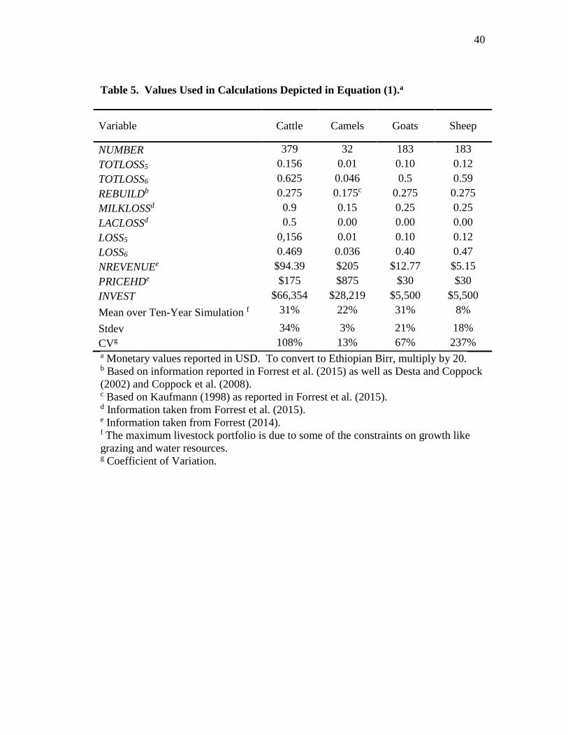
40
Table 5. Values Used in Calculations Depicted in Equation (1).a
Variable Cattle Camels Goats Sheep
NUMBER 379 32 183 183
TOTLOSS5 0.156 0.01 0.10 0.12
TOTLOSS6 0.625 0.046 0.5 0.59
REBUILDb 0.275 0.175c 0.275 0.275
MILKLOSSd 0.9 0.15 0.25 0.25
LACLOSSd 0.5 0.00 0.00 0.00
LOSS5 0,156 0.01 0.10 0.12
LOSS6 0.469 0.036 0.40 0.47
NREVENUEe $94.39 $205 $12.77 $5.15
PRICEHDe $175 $875 $30 $30
INVEST $66,354 $28,219 $5,500 $5,500
Mean over Ten-Year Simulation f 31% 22% 31% 8%
Stdev 34% 3% 21% 18%
CVg 108% 13% 67% 237% a Monetary values reported in USD. To convert to Ethiopian Birr, multiply by 20. b Based on information reported in Forrest et al. (2015) as well as Desta and Coppock
(2002) and Coppock et al. (2008). c Based on Kaufmann (1998) as reported in Forrest et al. (2015). d Information taken from Forrest et al. (2015). e Information taken from Forrest (2014). f The maximum livestock portfolio is due to some of the constraints on growth like
grazing and water resources. g Coefficient of Variation.

41
panel member of about $28,219 USD15 (Table 2). Total net revenue per head in a
normal16 year was estimated by Forrest (2014) on a per head basis17 to be about $205
USD per head (Table 3). This suggests total net revenue from milk and livestock
sales or consumption18 in a normal year from camels would be about $6,611 USD
(Table 3). During drought years, milk production is reduced by 15 percent for female
camels and (Coppock 1994; Coppock et al. 2014). Equation (1) can be used with the
information provided in Table 5 to calculate returns for the investment in camels over
the 10-year period.
Based on equation (1) and Table 5, it is estimated that the return on the value
of the camel herd (investment) would be about 23 percent ($6,611 /$28,219) during a
normal rainfall year. Two successive years of drought would result in approximately
4.58 percent loss of the camels herd based on average estimates made by the Panel.
Based on a suggestion by Coppock (personal conversation 2015), average returns to
the camels herd were calculated over a 10-year period assuming the first four years
15 Assumes an exchange rate of about 20 Birr per $1 USD (xe.com 2015).
16 “Normal” was defined by Forrest (2014) as a year with normal rainfall or, in other
words, a non-drought year.
17 Forrest (2014) estimated costs and returns on both a per head and per camel basis.
Per head basis is what is reported here.
18 Forrest (2014) valued both sales and consumption of livestock products (milk and
meat) at the market value to account for the opportunity costs of these products.

42
were normal rainfall years and provided a return of 23 percent to the investment in
camels. The fifth (Year 5) and sixth years (Year 6) were assumed to be drought years
with an absolute loss in the Camels herd by 4.6 percent divided into 1 percent during
the first year and 3.6 percent during the second year (Table 4).
Sheep19
The total number of sheep owned by the 12 members of the Panel was 750
males and 1450 females (Table 1). The average number per pastoralist is 63 males
and 121 Females (Table 2). This suggested that each Panel member owned an average
of about 63 males and 121 females or 184 sheep in total (Table 2). The value per head
was assumed to be $30 USD as reported in Forrest (2014). This gave an average
value for the sheep owned by each panel member of about $5,500 USD.20 Total net
revenue per head in a normal21 year was estimated by Forrest (2014) on a per head
19 During droughts milk production is reduced by 25 percent for the surviving female
sheep. The number of sheep is reduced by 59 percent divided in to 12 percent during
the first year and 47 percent during the second year. This is based on information
from the surveys, Coppock (personal conversation 2015) and Bailey (personal
conversation 2015) relating to droughts having less impacts in the first year of a
drought than in the second.
20 Assumes an exchange rate of about 20 Birr per $1 USD (xe.com 2015).
21 “Normal” was defined by Forrest (2014) as a year with normal rainfall or, in other
words, a non-drought year.

43
basis22 to be about $5 USD per head (Table 3). This suggested that total net revenue
from milk and livestock sales or consumption23 in a normal year from sheep would be
about $944 USD (Table 3). This suggested a return on the value of the sheep flock
(investment) of about 17 percent ($944/$5,500) during a normal rainfall year.
Two successive years of drought would result in approximately 59 percent
loss of the sheep flock based on average estimates made by the Panel (Table 4).
Based on a suggestion by Coppock (personal conversation 2015), average returns to
the sheep flock were calculated over a 10-year period assuming the first four years
were normal rainfall years and provided a return of 17 percent to the investment in
sheep. The fifth (Year 5) and sixth years (Year 6) were assumed to be drought years
with an absolute loss in the sheep flock of 12 percent during the first year and 47
percent during the second year.
During drought years, milk production for sheep was assumed to decline by
25 percent and 0 percent of the remaining female sheep had lambs (actually lactated).
As a result, returns for sheep during the drought years were calculated based on
equation (1) and the information given in Table 5. These estimated returns are
calculated for the 10-year period for sheep and are reported in Table 4.
22 Forrest (2014) estimated costs and returns on both per head and per cow basis. Per
head basis is what is reported here.
23 Forrest (2014) valued both sales and consumption of livestock products (milk and
meat) at the market value to account for the opportunity costs of these products.

44
Goats24
The total number of goats owned by the 12 members of the Panel was 750
males and 1450 females (Table 1). The average number per pastoralist is 63 males
and 121 Females (Table 2). This suggested that each Panel member owned an average
of about 63 males and 121 females or 184 goats in total (Table 2). The value per head
is assumed to be $30 USD as reported in Forrest (2014). This gives an average value
for the goats owned by each panel member of about $5,500 USD (Table 2).25 Total
net revenue per head in a normal26 year was estimated by Forrest (2014) on a per head
basis27 to be about $13 USD per head for goats (Table 3). This suggested that total
24 During droughts milk production is reduced 25 percent for the surviving female
goats during. The number of goats is reduced by 50 percent divided in to 10 percent
during the first year and 40 percent during the second year. This is based on
information from the surveys, Coppock (personal conversation 2015) and Bailey
(personal conversation 2015) relating to droughts having less impacts in the first year
of a drought than in the second.
25 Assumes an exchange rate of about 20 Birr per $1 USD (xe.com 2015).
26 “Normal” was defined by Forrest (2014) as a year with normal rainfall or, in other
words, a non-drought year.
27 Forrest (2014) estimated costs and returns on both per head and per cow basis. Per
head basis is what is reported here.

45
net revenue from milk and livestock sales or consumption28 in a normal year from
goats would be about $2,341 USD (Table 3). This suggested a return on the value of
the goats herd (investment) of about 43 percent ($2340/$5,500) during a normal
rainfall year (Table 4).
Two successive years of drought would result in approximately 50 percent
loss of the goat herd based on average estimates made by the Panel (Table 4). Based
on a suggestion by Coppock (personal conversation 2015), average returns to the goat
herd were calculated over a 10-year period assuming the first four years were normal
rainfall years and provided a return of 42.6 percent to the investment in goats (Table
4). The fifth (Year 5) and sixth years (Year 6) were assumed to be drought years with
an absolute loss in the goats herd of 10 percent during the first year and 40 percent
during the second year. The information provided on Table 5 is applied to calculate
returns to the goat herd over the 10-year period and these returns are reported in
Table 4.
Crops
The returns on crops are calculated using a return on assets (ROA) approach
based on the survey questionnaire and the data provided by the 12 members of the
Panel. The revenues and costs (income) for livestock portfolio are derived from
28 Forrest (2014) valued both sales and consumption of livestock products (milk and
meat) at the market value to account for the opportunity costs of these products.

46
Forrest (2014) conducted in the Harweyu community of the Borana Plateau region
compared to the assets held by the 12 members of the panel.
Crops in the survey region are dominated by maize and beans (Coppock et al.
2014) and this matches what the 12 members of the Panel indicated. The total number
of hectares (ha.) of cropland farmed by the 12 members of the Panel was 20 ha. This
20 ha. is divided between 15.4 ha. of maize and 4.6 ha. of haricot beans (Table 6).
The average amount of cropland farmed per pastoralist is 1.67 ha. (Table 7).
Maize
The price of maize is $ 0.2 USD/kg for the crop and $0.1 USD/kg for maize
residue (Forrest 2014). This gave an average value for the maize owned by each panel
member of about $647.03 USD (Table 7). The following equation is used to calculate
returns for crops:
(2) 𝑅𝐸𝑇𝐶𝑅𝑂𝑃𝑐𝑡 = ((𝑌𝐼𝐸𝐿𝐷𝑐)(𝐶𝑅𝑂𝑃𝑃𝑅𝑐𝑡) + 𝑅𝐸𝑆𝐼𝐷𝑈𝐸𝑉𝐿𝑐𝑡 −
𝐸𝑋𝑃𝐸𝑁𝑆𝐸𝑆𝑐𝑡)/𝐸𝑋𝑃𝐸𝑁𝑆𝐸𝑆𝑐𝑡
where RETCROPct was the return on crop investment in decimal form for the cth crop
(c = maize, beans) in the tth year. YIELD is the per hectare yield, CROPPR is the crop
price, RESIDUEVL was the value of crop residue, and EXPENSES were the expenses
reported for these crops by Forrest (2014). For drought years (t = 5, 6), YIELD and
RESIDUEVL were assumed to equal zero. A land charge of 150 Birr ($7.50) per
hectare was included in this case that was not included in Forrest (2014). The mean
return and itsσ for RETCROP for the different crops as calculated over a simulated

47
ten-year period was used to simulate a distribution of returns used in the stochastic
dominance analysis explained later. Using equation (2), an average return on land
and management for normal year is about $ 470.43 USD (Table 7) for maize. This
suggested an average return on land and management for drought year is about $ -
161.74 USD (Table 7).
Two successive years of drought would result in a 100 percent loss of the
maize harvest. Based on a suggestion by Coppock (2015), average returns to the
maize crop were calculated over a 10-year period assuming the first four years were
normal rainfall years and provided a return of 240.23 percent (Table 8). The fifth
(Year 5) and sixth years (Year 6) were assumed to be drought years with an absolute
loss of the whole crop and residue. Table 9 reports numbers used in the calculations
reported in Table 8.
Haricot Beans
The price of Haricot Beans is $ 0.20 USD/kg for the crop and $0.10 USD/kg for
haricot beans residue (Forrest 2014). This gave an average value for the haricot beans
owned by each panel member of about $348.80 USD (Table 7). This suggested an
average return on land and management for normal year is about $295.45/ha. USD
(Table 7). This suggested an average return on land and management for drought
year is about $48.88 USD (Table 7).

48
Table 6. Total Crop Land Share and Returns of Cropland Per Member of the Panel.a
Crop
Total
croplan
d Ha.
Crop share
Ha.b
Quantit
y
kg
Price/k
g
USD
Crop Net
value
Birr/Ha.c
Total
Value in
Birr
Total
Return to
Land and
Managemen
t Normal
Year
Total Return
to Land and
Management
in Drought
Year
Maize
20 15.375
2000 $0.20 400
7764.38 5645.13 -1940.89 Residue 1125 $0.10 112.5
Beans
4.625
4000 $0.20 800
4185.63 3545.42 -586.55 Residue 1125 %0.10 112.5
a Monetary values reported in USD. To convert to Ethiopian Birr, multiply by 20. b The crop share of land assuming that about 75 percent of the land is cropped with maize and 25 percent with beans (Tezera
2014). c Based on that reported in Forrest (2014). During drought years no labor cost for harvest is excluded and EXPENSES was
reduced by $26.60/ha. in those years (see equation (2). In addition to expenses listed in Forrest (2014) a 150 Birr land rent
change was also subtracted from gross revenues. The rental rate was based on an average from rental rates across Ethiopia as
reported by the Ethiopian Ministry of Agriculture (2015).
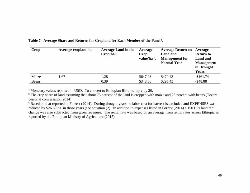
49
Table 7. Average Share and Returns for Cropland for Each Member of the Panela.
Crop Average cropland ha Average Land in the
Crop/hab.
Average
Crop
value/ha c.
Average Return on
Land and
Management for
Normal Year
Average
Return to
Land and
Management
in Drought
Years
Maize 1.67 1.28 $647.03 $470.43 -$161.74
Beans 0.39 $348.80 $295.45 -$48.88
a Monetary values reported in USD. To convert to Ethiopian Birr, multiply by 20. b The crop share of land assuming that about 75 percent of the land is cropped with maize and 25 percent with beans (Tezera
personal conversation 2014). c Based on that reported in Forrest (2014). During drought years no labor cost for harvest is excluded and EXPENSES was
reduced by $26.60/ha. in those years (see equation (2). In addition to expenses listed in Forrest (2014) a 150 Birr land rent
change was also subtracted from gross revenues. The rental rate was based on an average from rental rates across Ethiopia as
reported by the Ethiopian Ministry of Agriculture (2015).
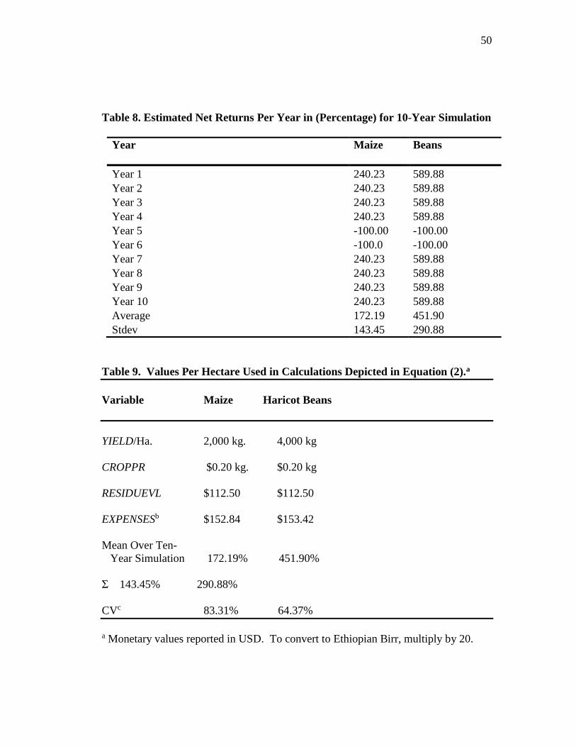
50
Table 8. Estimated Net Returns Per Year in (Percentage) for 10-Year Simulation
Year
Maize
Beans
Year 1 240.23 589.88
Year 2 240.23 589.88
Year 3 240.23 589.88
Year 4 240.23 589.88
Year 5 -100.00 -100.00
Year 6 -100.0 -100.00
Year 7 240.23 589.88
Year 8 240.23 589.88
Year 9 240.23 589.88
Year 10 240.23 589.88
Average 172.19 451.90
Stdev 143.45 290.88
Table 9. Values Per Hectare Used in Calculations Depicted in Equation (2).a
Variable Maize Haricot Beans
YIELD/Ha. 2,000 kg. 4,000 kg
CROPPR $0.20 kg. $0.20 kg
RESIDUEVL $112.50 $112.50
EXPENSESb $152.84 $153.42
Mean Over Ten-
Year Simulation 172.19% 451.90%
Σ 143.45% 290.88%
CVc 83.31% 64.37%
a Monetary values reported in USD. To convert to Ethiopian Birr, multiply by 20.

51
b EXPENSES based on that reported in Forrest (2014). During drought years no labor
cost for harvest is included and EXPENSES was reduced by $26.60 in those years. c Coefficient of Variation.
Two successive years of drought would result in a 100 percent loss of the haricot
bean harvest. Based on a suggestion by Coppock (2015), the average returns to the
haricot bean crop are calculated over a 10-year period assuming the first four years
are normal rainfall years and provided a return of 589.88 percent (Table 8). The fifth
(Year 5) and sixth years (Year 6) were assumed to be drought years with an absolute
loss of the whole crop and residue. Table 8 reports estimated returns for haricot
beans over a 10-year period based on equation (2) and the information given in Table
9.
Real Estate
Access Capital is an Ethiopian company that creates reports to support
investing in Ethiopia. They surveyed three residential real estate brokers in each of
10 residential neighborhoods of Addis Ababa focusing on the sales price and monthly
rent for individual homes. They measured returns on real estate by comparing it to the
annual rental income derived from a property relative to its purchase price. The yield
according to the report varies depending on size of the property and the
neighborhood. The rental yield around lower-priced neighborhoods in Addis Ababa
ranges from 4 to 5 percent return per year. The report compares the yield in the case
of poorer neighborhoods to be similar to that received on saving accounts. Returns of
high-priced neighborhoods in Addis Ababa are around 10 percent (Access Capital
2010).
52
Leamer (2007) and others researched and analyzed the effects of GDP on
housing prices. Valadez (2010) investigated the relationship and correlation between
house prices indexes (HPI) and the change of GDP in the United States. The results
of his research suggested that there is a positive relationship between HPI and GDP.
The average of the Ethiopia GDP growth (annual percentage) 2003-2012 is 9.82
percent with a σ of ±4.22 percent. Given that no information was available for
returns to real estate investment in the Borana Plateau, it was decided a more reliable
measure of return on real estate investment would be changes in Ethiopia’s GDP and
the information reported in Table 10 is what is used to complete the investment
portfolio analysis in this study.
Bank Saving Accounts
In 2011 the average saving deposit rate for public banks in Ethiopia was four
percent and for private banks was six percent. The lending rate from public banks
was 9.5 percent and private banks was 12.5 percent during this same time period
(World Bank 2013). One percent of rural Ethiopian households have bank accounts.
Fourteen percent of the adult population in Ethiopia has access to credit. The average
loan amount in 2010 in Ethiopia was US$ 170 (World Bank 2013). The saving
account earns an interest of 5 percent compounded and calculated basis (Commercial
Bank of Ethiopia 2015), according to the National Bank of Ethiopia, The average
interest rate between 2003 and 2013 was 3.73 percent with a σ of ±0.79 percent and
this is what was used to complete the portfolio analysis in this study.

53
Risk Perception
In an attempt to measure the perception of risk for different investment options, the
12 panel members were asked to rank their investment options over a period of 10
years from the investment perceived to be the most risky (ranked #1) to the one
perceived to be the least risky (ranked #4). To get a general perception of perceived
risk in different categories of assets, livestock, banking, property in town, and
cultivation were the choices for these rankings provided to the Panel. Perhaps not
surprisingly, the Panel ranked livestock investment as the most risky followed by
cultivation, banking and real estate (Table 11). The 12 panel members were also
asked to rank their perceptions of the relative risk of investing in the different
livestock species (cattle, camels, goats, and sheep). They ranked cattle as the riskiest
livestock species followed by sheep, goats and camels (Table 12).
The panel members compared their perception of risk of other investments
compared to their perceptions of the risk associated with livestock over a period of 10
years. The majority saw banking as less risky than livestock (Table 13). They were
equally divided to see real estate as two times less risky and five times less risky than
the livestock (Table 13). Cropland came in as being as risky as livestock (Table 13).
Portfolio and Investment Selection
The investment portfolios, based on percentage invested in each of the
investment options considered, for the 12 panel members is reported in Table 14. The
average share and σ (risk) of each of the investments indicated by the panel members
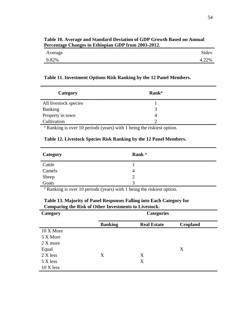
54
Table 10. Average and Standard Deviation of GDP Growth Based on Annual
Percentage Changes in Ethiopian GDP from 2003-2012.
Average Stdev
9.82% 4.22%
Table 11. Investment Options Risk Ranking by the 12 Panel Members.
Category Ranka
All livestock species 1
Banking 3
Property in town 4
Cultivation 2 a Ranking is over 10 periods (years) with 1 being the riskiest option.
Table 12. Livestock Species Risk Ranking by the 12 Panel Members.
Category Rank a
Cattle 1
Camels 4
Sheep 2
Goats 3 a Ranking is over 10 periods (years) with 1 being the riskiest option.
Table 13. Majority of Panel Responses Falling into Each Category for
Comparing the Risk of Other Investments to Livestock.
Category Categories
Banking Real Estate Cropland
10 X More
5 X More
2 X more
Equal X
2 X less X X
5 X less X
10 X less

55
is also reported in Table 14 and will be compared with the results from the optimum
portfolio selection and share as determined by the quadratic programing analysis
reported later on.
Cattle are the Panel’s largest investment (average of 35 percent of the total
portfolio with a σ of ±16.90 percent). The average share of real estate is 22.16 percent
with a σ of ±17.55 percent. Camel’s average share is 12.89 percent with a σ of ±8.85
percent. Bank accounts average share is 12.89 percent with a σ of ±8.85 percent. The
average share for sheep is 3.81 with a σ of ±2.09 percent. Maize’s average share is
0.14 percent with a σ of ±0.1 percent and at the investment share for beans was the
smallest of the options considered at an average share of 0.04 percent and a standard
of 0.03 percent. When one considers the average of investment in livestock (summing
investment across cattle, camels, goats, and sheep), one can see that the Panel
maintains approximately two-thirds of its assets in livestock investments, on the
average. Real estate is far-and-away the most popular investment after livestock
based on the average proportion of the total portfolio invested in real estate (Table
14). Many of the Panel members indicated that their real estate investments are
related primarily to housing for family members. Bank accounts are not heavily
preferred and crops, which have a high variability of returns, are also not overly
preferred by the Panel. These results suggest a fairly sophisticated understanding of
risks and returns to different investments. This statement is based on the fact that
investment flows not simply to the least risky assets to avoid risk, such as bank
accounts, but is also spread across livestock species and real estate.
56
The following chapter presents an analysis of the data related in the various
investments chosen by the Panel members. The purpose of the analysis is to
determine the “optimality” of the investment choices of the Panel in terms of risk and
risk preferences. This type of analysis is appropriate given the different investment
choices displayed across members of the Panel. It also aids researchers in
understanding the diversification strategies of wealthy pastoralists which may assist
in the understanding of how to encourage portfolio diversification on the Borana
Plateau. It may also aid in helping to delineate policy strategies for encouraging
investment that will lead to locally-led economic development on the Borana Plateau.

57
Table 14. Estimated Share of Total Portfolio in (Percentage) for Each
Investment Category for Each Panel Participant Together with Average and
Standard Deviation for the Entire Panel.
Participant
Bank
Account Cattle Camels Goats Sheep
Real
Estate Maize Beans
P1 20.00 67.67 8.46 0.87 0.87 2.08 0.04 0.01
P2 9.09 43.94 27.46 7.53 7.53 4.08 0.27 0.09
P3 4.76 36.77 18.39 6.30 6.30 27.32 0.11 0.04
P4 16.67 20.26 0.00 3.47 3.47 55.79 0.25 0.08
P5 0.00 31.38 52.30 3.59 3.59 8.97 0.13 0.04
P6 16.67 19.06 23.82 3.27 3.27 33.76 0.12 0.04
P7 16.67 28.88 36.10 4.95 4.95 8.46 0.00 0.00
P8 9.09 18.66 18.66 3.20 3.20 46.92 0.19 0.06
P9 9.09 52.42 26.21 3.00 3.00 5.99 0.22 0.07
P10 9.09 38.33 23.96 4.93 4.93 18.69 0.06 0.02
P11 34.43 11.97 20.52 0.00 0.00 32.83 0.25 0.00
P12 9.09 53.91 6.74 4.62 4.62 21.02 0.00 0.00
Average 12.89% 35.27% 21.88% 3.81% 3.81% 22.16% 0.14% 0.04%
Stdev 8.85% 16.90% 13.81% 2.09% 2.09% 17.55% 0.10% 0.03%
58
CHAPTER 4
RISK ANALYSIS AND RESULTS
The analysis used in this study relying on methods taking into account rates of
return, risks associated with returns, and risk bearing preferences for different
decision makers. The methods applied are well-known and frequently used in these
types of analyses. The innovation in this study lies in the data obtained from the
Panel and the insights that can be gained using the data in the analyses. These
insights will help in understanding the investment opportunities, choices, and risks
facing wealthy pastoralists on the Borana Plateau. The investment choices of wealthy
pastoralists have the potential to significantly influence economic development in the
study area. As a result, the understanding the motivations and choices of these
pastoralists in their investment choices is important to everyone living in the study
area.
Risk Analysis Based on Survey Reponses
The analysis relies on estimated empirical (observed) distributions on returns
to eight investment choices (Table 4).29 Four of these choices are related to livestock
(cattle, camels, goats, and sheep), two to non-agricultural investments (real estate and
bank savings accounts), and two are related to crop investment (maize and beans).
29 See also equations (1) and (2) for how the empirical distributions reported in Table
4 were estimated.

59
Having empirical distributions provides an avenue for risk analysis through
the use of simulation. Essentially, one can incorporate uncertainty into the analysis
by assuming a distribution of returns (in this case an empirical distribution) and then
“simulating” many possible outcomes (returns) that might result between the
extremes indicated by the empirical distribution. This assumes, of course, that all
possible returns or outcomes are represented by the empirical distribution. While this
qualifies the interpretation of the results of the analysis because it is possible for more
extreme events to happen than indicated by the Panel participants, it avoids assuming
some type of theoretical distributions (e.g., normal distribution) that may or may not
actually fit the reality of investment returns in the study area.
Risk analysis requires that the distribution of returns to different investments
must be accompanied by assumptions for the utility functions of decision makers who
make portfolio choices among different possible investments. Decision makers are
assumed to maximize their utility based on their utility function (Norstad 2011).
Because the utility function incorporates the influence of wealth as well as its trade-
offs with risk (uncertainty), maximizing utility allows for the identification of
“optimal” portfolio selection based on these trade-offs. In this study we employ the
negative exponential utility function as the basis for portfolio selection for wealthy
pastoralists (Norstad 2011). The negative exponential utility function may be
represented as follows:
(3) 𝑈(𝑤) = −𝑒−𝜌𝑤

60
where w represents either consumption or wealth and 𝜌 is degree of risk preference of
the decision maker. If 𝜌 = 0 then the decision maker is said to be “risk neutral.” If 𝜌
> 0 the decision maker is said to be “risk averse,” and if 𝜌 < 0 the decision maker is
said to be “risk preferring” or “risk seeking” (Moss 2010). The level of risk
preference is important because it drives the “shape” of the utility function and the
decision maker’s choice based on risk. Specifically, this can be shown by the relative
“curve” of the utility function that can be determine by the ratio of the first and
second derivatives of the utility function.
(4) 𝑈′(𝑤) = −𝜌𝑒−𝜌𝑤
(5) 𝑈′′(𝑤) = −𝜌2𝑒−𝑤
The ratio of the first and second derivative of provides the “relative” risk preference
of the decision maker and is called the Arrow-Pratt absolute risk aversion coefficient
(RAC). It is calculated as follows:
(6) 𝑅𝐴𝐶 = − [−𝜌2𝑒−𝑤
−𝜌𝑒−𝜌𝑤] = 𝜌
Equation (6) demonstrates that for the negative exponential utility function that the
RAC is identified by a single number 𝜌 that can also be referred to as a constant
absolute risk aversion coefficient or CARA as a result. The analysis will present
preferred investment portfolios over a range of values for the RAC. This allows for
understanding how risk preference influences the investment choices that are made by
wealthy pastoralists and also can provide information for how choices might vary as
the level of risk associated with different investments changes.

61
Stochastic Dominance Analysis
Given there are many different investment combinations that could go into the
portfolios of wealthy pastoralists, a method or methods needs to be applied to decide
which of these risky choices should not be considered (are not in the “efficient set” of
alternatives). Stochastic dominance with respect to a function (SDRF) (Meyer 1977a
and b) has been frequently used to make pair-wise comparisons among different
investment alternatives to determine an efficient set. Hadar and Russell (1969)
provide definitions for first and second degree stochastic dominance. First degree
stochastic dominance (FSD) is defined as follows:
The probability function g is said to be at least as large as f in the sense of
FSD if and only if G(X) ≤ F(X) for all x in the set of real numbers. Where G
and F represent the cdfs of f and g, respectively. The function g is said to be
larger than f in the sense of FSD if and only if the above inequality bolds
strictly fo at least one x.
In other words, this definition indicates that if two cdfs (G and F) are graphed and
compared, that if G is FSD over F if it lies completely (no cross-overs) to the left of
F. The definition provided for second-degree stochastic dominance (SSD) by Hadar
and Russell (1969) is the following:
The probability function g is said to be at least as large as f in the sense of
SSD if and only if ∫ 𝐺(𝑡)𝑑𝑡 ≤ ∫ 𝐹(𝑡)𝑑𝑡𝑥
𝑎
𝑥
𝑎 for all x as an element of the real
numbers set. The function g is said to be larger than f in the sense of SSD if
and only if the above inequality holds strictly for at least one x (p. 289).
In other words, SSD refers to SSD being defined over a set area of two cdfs where G
lies to the left of F. Computer programs can be used to test for FSD and SSD. The
one employed in this analysis is in Simetar (Richardson et al. 2006). The analysis
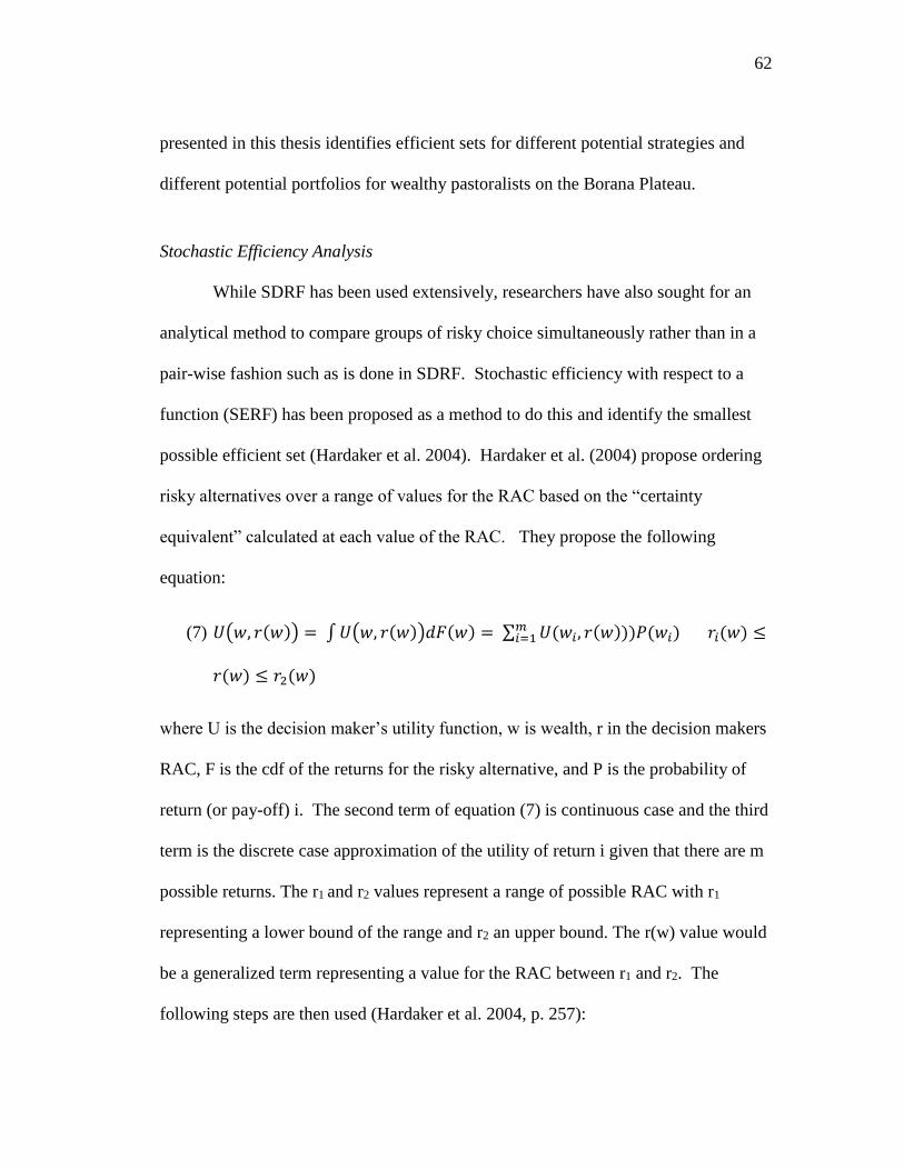
62
presented in this thesis identifies efficient sets for different potential strategies and
different potential portfolios for wealthy pastoralists on the Borana Plateau.
Stochastic Efficiency Analysis
While SDRF has been used extensively, researchers have also sought for an
analytical method to compare groups of risky choice simultaneously rather than in a
pair-wise fashion such as is done in SDRF. Stochastic efficiency with respect to a
function (SERF) has been proposed as a method to do this and identify the smallest
possible efficient set (Hardaker et al. 2004). Hardaker et al. (2004) propose ordering
risky alternatives over a range of values for the RAC based on the “certainty
equivalent” calculated at each value of the RAC. They propose the following
equation:
(7) 𝑈(𝑤, 𝑟(𝑤)) = ∫ 𝑈(𝑤, 𝑟(𝑤))𝑑𝐹(𝑤) = ∑ 𝑈(𝑤𝑖, 𝑟(𝑤)))𝑃(𝑤𝑖) 𝑟𝑖(𝑤) ≤𝑚𝑖=1
𝑟(𝑤) ≤ 𝑟2(𝑤)
where U is the decision maker’s utility function, w is wealth, r in the decision makers
RAC, F is the cdf of the returns for the risky alternative, and P is the probability of
return (or pay-off) i. The second term of equation (7) is continuous case and the third
term is the discrete case approximation of the utility of return i given that there are m
possible returns. The r1 and r2 values represent a range of possible RAC with r1
representing a lower bound of the range and r2 an upper bound. The r(w) value would
be a generalized term representing a value for the RAC between r1 and r2. The
following steps are then used (Hardaker et al. 2004, p. 257):

63
1. Select points on each CDF for a finite set of values of w.
2. Convert each of these w values to its utility using the selected for of utility
function and the selected value of the risk aversion coefficient.
3. Multiply each finite utility by its associated probability to calculate a weighted
average of the utilities of outcomes.
This yields values in terms of the level of utility. Taking the inverse of the utility
function yields the “certainty equivalent” or CE. This can be represented as follows:
(8) 𝐶𝐸(𝑤, 𝑟(𝑤)) = 𝑈−1(𝑤, 𝑟(𝑤))
The CE represents the value of a “sure” return (investment) that yields the same
utility as expected return of a risky alternative (Hardaker et al. 2004; Helmberger and
Chavas 1996). In other words, what would the value of a sure return need to be to
make a decision maker indifferent between the risky investment and the sure
investment? The difference between the expected return for a risky investment and
the CE is something called the “risk premium” or RP. In other works an expected
return for a risky investment E(w) = CE + RP. The RP represents the amount of
money a decision maker would be willing to pay (WTP) to avoid the risky investment
if a sure investment is available. Based on this discussion and equation (8), the CE
and RP depend on the risk of an investment, the decision maker’s utility function, and
the decision maker’s RAC. For example, if the expected return on a risky investment
is $30 and the potential investor would be indifferent between the risky investment
($30) and another sure investment returning $20, the CE would be $20 and the RP
would be $10.
The SERF analysis presented in this thesis depicts the CEs and RPs for the
different investments and portfolios of investments for wealthy pastoralists on the

64
Borana Plateau. A negative exponential utility function is assumed in the analysis
and the SERF is conducted over a range of RACs representing from risk averse to
risk seeking decision makers. Consequently, the RAC is defined over a range similar
range. Following a modified method for determining the RAC as suggested by
(McCarl and Bessler 1989; Richardson 2006). The RAC was calculated as:
(9) 𝑅𝐴𝐶 = ± 5
𝑆𝑡𝐷𝑒𝑣.
Nonlinear Programming Analysis
A nonlinear programming (NLP) model is used to create optimum portfolios
based on the eight different investment choices considered for wealthy pastoralists
and five different sets of restrictions (Hazell and Norton 1986; Hardaker et al. 2004).
NLP assumes wealthy pastoralists are risk averse and will only choose an investment
with a higher expected return if the variance of the investment is also greater
compared to another investment. The NLP model is chosen to rank the investment
choices according to the risk and return without using a utility function (Hardaker et
al. 2004; Mapp et al. 1979; Manos and Kistopanidis 1986). Nonlinear programming
is a process that allows a decision maker to optimize (maximize or minimize) an
objective function subject to a number of constraints that are nonlinear. A generic
notation for a non-linear programing is shown as follows (Bradley et al. 1977, p.
410):
Minimize
(10) 𝑓 (𝑥1, 𝑥2, … , 𝑥𝑛) ,

65
subject to:
(11) 𝑔1(𝑥1, 𝑥2, … , 𝑥𝑛) ≤ 𝑏1 ,
⋮ ⋮
𝑔𝑚(𝑥1, 𝑥2, … , 𝑥𝑛) ≤ 𝑏𝑚 ,
where the constraint functions 𝑔1through 𝑔𝑚 are given and do not need to be linear.
The total for investment shares must sum to one. The NLP is optimized assuming
that the variance of returns is minimized for five separate investment portfolios
defined by the constraints placed on maximum investments in an single investment
option. For this study, the five separate scenarios considered for the NLP are the
following (see Table 15):
(a) Unrestricted (PUR) – a portfolio with no restriction on how much of the
pastoralists total assets could be invested in any one of the eight
investments choice.
(b) 2nd Data (P2D) – Survey data. This portfolio option uses limits suggested
by Dr. Coppock (personal communication 2015) as resource constraints.
For example, full utilization of grass and grazing constraints requires a
complements of cattle, camels, and small ruminants. Information on
carrying capacities for different livestock species in Harweyu were
provided in Forrest et al. (2015). The proportions of the livestock species
represented at carrying capacity for Harweyu were used as the constraints
on the proportions of the different livestock species that could be part of
the portfolio.

66
(c) Survey Max (PSM) - This portfolio option uses the maximum level of
investment by a single one of the 12 Panel members as the maximum
amount any of the 12 Panel members could invest in a single one of the
eight investment choices.
(d) Equal (PE) - This portfolio option assumes equal proportions of total
assets are invested across the investment options considered.
(e) Max Diversity (PMD) - this profile option uses a recommendation by most
financial authorities that no more than 20 percent should be invested in
any single investment category to avoid unnecessary amounts of risk.
A description of the constraints for each of the five investment strategies
described above, the variance-covariance matrix used in the NLP model, and the
optimal portfolios associated with each strategy are provided in Tables 15, 16, and 17,
respectively. The optimum investment portfolios identified for each of the five
investment strategies (restriction sets) are used later in the analysis as a basis for
determining how the different constraints affect investment behavior and place limits
on the ability to adjust investments in the face of risk.
Simulation Analysis
The basis for the simulation begins with developing the cumulative density
functions (cdfs) for the different investment alternatives for the 10 years described in
Table 4 (Table 18). Correlated uniform standard deviates (CUSD) are developed to
conduct the simulation by randomly drawing 500 uniform standard deviates from a U

67
Table 15. Synopsis of Constraints in the Nonlinear Programming Model
Imposed for Five Separate Strategies.
Maximum Investment in (percentage)
Strategya Cattle Camels Goats Sheep Crops Savings Real
Estate
PUR 100 100 100 100 100 100 100
P2D 63 27 5 5 5 50 50
PSM 68 52 8 8 >1 34 56
PE 14 14 14 14 14 14 14
PMD 20 20 20 20 20 20 20
a PUR = no restrictions on amount of portfolio in each investment option. P2D =
total investment in each option limited by resources available. PSM = total
investment in each option constrained to be no larger than the largest percentage
invested by an individual member of the panel in that option. PE = investments
constrained to be equal across all investment options. PMD = investments
constrained to be no more than 20 percent of total portfolio in any single investment
option.
Table 16. Variance-Covariance Matrix Associated With the Nonlinear
Programming Model Used in the Analysis.
Cattle Camels Goats Sheep Savings Real
Estate
Maize Beans
Cattle 0.1037 0.0084 0.0620 0.0530 -0.0006 0.0022 0.4040 0.8193
Camels 0.0084 0.0007 0.0052 0.0045 -0.0000 0.0002 0.0350 0.0710
Goats 0.0620 0.0052 0.0400 0.0346 -0.0002 0.0013 0.2295 0.4653
Sheep 0.0530 0.0045 0.0346 0.0304 -0.0002 0.0013 0.1961 0.3976
Savings -0.0006 -0.0000 -0.0002 -0.0002 0.0001 -0.0001 -0.0014 -0.0028
Real
Estate 0.0022 0.0002 0.0013 0.0013 (0.0001) 0.0002 0.0083 0.0168
Maize 0.4040 0.0350 0.2295 0.1961 (0.0014) 0.0083 1.8521 3.7555
Beans 0.8193 0.0710 0.4653 0.3976 (0.0028) 0.0168 3.7555 7.6149
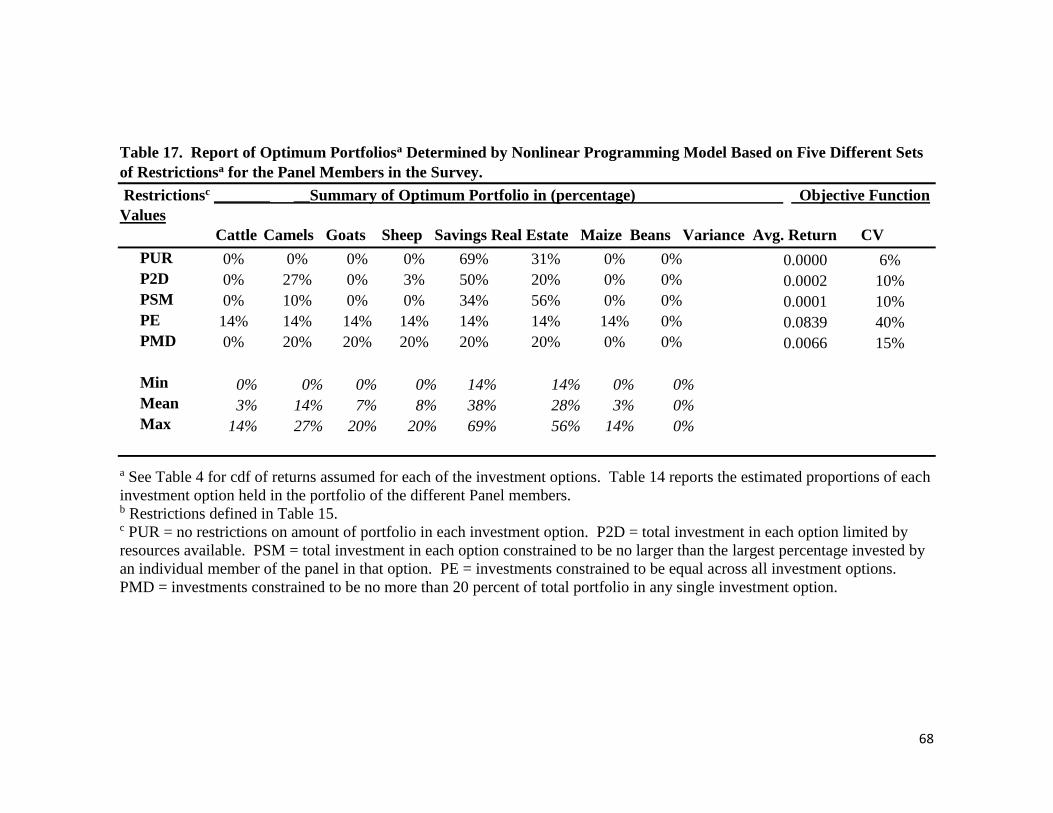
68
Table 17. Report of Optimum Portfoliosa Determined by Nonlinear Programming Model Based on Five Different Sets
of Restrictionsa for the Panel Members in the Survey.
Restrictionsc _______ __Summary of Optimum Portfolio in (percentage) Objective Function
Values
Cattle Camels Goats Sheep Savings Real Estate Maize Beans Variance Avg. Return CV
PUR 0% 0% 0% 0% 69% 31% 0% 0% 0.0000 6%
P2D 0% 27% 0% 3% 50% 20% 0% 0% 0.0002 10%
PSM 0% 10% 0% 0% 34% 56% 0% 0% 0.0001 10%
PE 14% 14% 14% 14% 14% 14% 14% 0% 0.0839 40%
PMD 0% 20% 20% 20% 20% 20% 0% 0% 0.0066 15%
Min 0% 0% 0% 0% 14% 14% 0% 0%
Mean 3% 14% 7% 8% 38% 28% 3% 0%
Max 14% 27% 20% 20% 69% 56% 14% 0%
a See Table 4 for cdf of returns assumed for each of the investment options. Table 14 reports the estimated proportions of each
investment option held in the portfolio of the different Panel members. b Restrictions defined in Table 15. c PUR = no restrictions on amount of portfolio in each investment option. P2D = total investment in each option limited by
resources available. PSM = total investment in each option constrained to be no larger than the largest percentage invested by
an individual member of the panel in that option. PE = investments constrained to be equal across all investment options.
PMD = investments constrained to be no more than 20 percent of total portfolio in any single investment option.
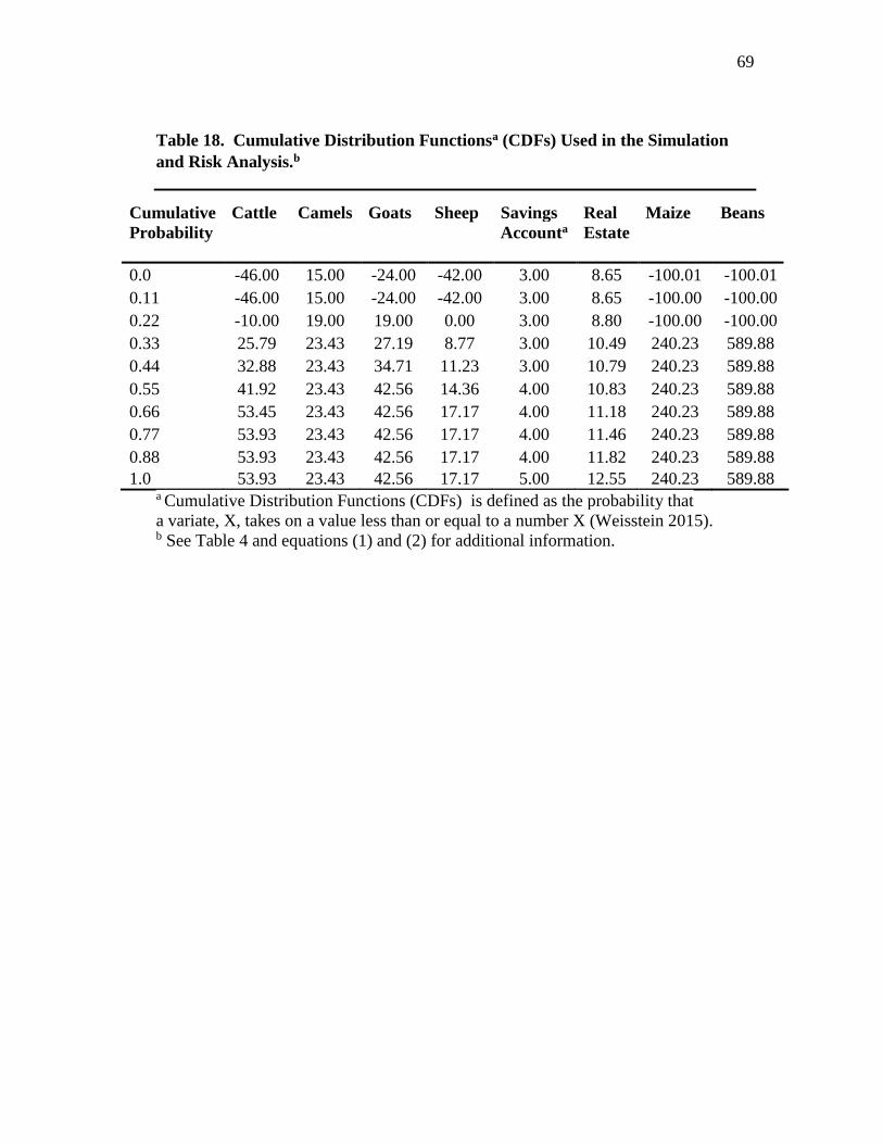
69
Table 18. Cumulative Distribution Functionsa (CDFs) Used in the Simulation
and Risk Analysis.b
Cumulative
Probability
Cattle Camels Goats Sheep Savings
Accounta
Real
Estate
Maize Beans
0.0 -46.00 15.00 -24.00 -42.00 3.00 8.65 -100.01 -100.01
0.11 -46.00 15.00 -24.00 -42.00 3.00 8.65 -100.00 -100.00
0.22 -10.00 19.00 19.00 0.00 3.00 8.80 -100.00 -100.00
0.33 25.79 23.43 27.19 8.77 3.00 10.49 240.23 589.88
0.44 32.88 23.43 34.71 11.23 3.00 10.79 240.23 589.88
0.55 41.92 23.43 42.56 14.36 4.00 10.83 240.23 589.88
0.66 53.45 23.43 42.56 17.17 4.00 11.18 240.23 589.88
0.77 53.93 23.43 42.56 17.17 4.00 11.46 240.23 589.88
0.88 53.93 23.43 42.56 17.17 4.00 11.82 240.23 589.88
1.0 53.93 23.43 42.56 17.17 5.00 12.55 240.23 589.88 a Cumulative Distribution Functions (CDFs) is defined as the probability that
a variate, X, takes on a value less than or equal to a number X (Weisstein 2015). b See Table 4 and equations (1) and (2) for additional information.

70
Table 19. Estimated Net Returns in (Percentage) Per Year for the 10-Year
Simulation Reported in Percentages.
Year Cattle Camels Goat
s
Shee
p
Savings
Accounta
Real
Estat
e
Maize Bean
s
1 54 23 43 17 3 14 240 590
2 54 23 43 17 3 12 240 590
3 54 23 43 17 3 11 240 590
4 54 23 43 17 3 11 240 590
5 -10 19 19 0 4 11 -100 -100
6 -46 15 -24 -42 4 9 -100 -100
7 26b 23c 27 9 4 13 240 590
8 33 23 35 11 4 11 240 590
9 42 23 43 14 5 9 240 590
10 53 23 43 17 5 10 240 590
Avg. 31 22 31 8 4 11 172 452
Stdev 34 3 21 18 1 2 143 291
CVd 108 13 67 237 21 14 83 64 a For savings account rates Year 1 corresponds with actual rates for 2003, Year 2 with
2004, and so forth to Year 10=2013 as reported by Trading Economics (2015). b The compounded annual rebuilding rate for numbers of cattle, sheep and goats
following a drought is approximately 27.5 percent (Desta and Coppock 2002) c The compounded annual growth in numbers for camels is approximately 17 percent
as reported in Forrest et al. (2015) based on Kaufmann (1998). d CV is coefficient of variation which is ratio of σ to the mean and used in
normalization of risk across multiple investments.

71
Table 20. Linear Correlation Matrix Used to Correlate Uniform Standard
Deviates in the Simulation Analysis.
Cattle Camel
s
Sheep Goat
s
Savings Real
Estate
Maize Beans
Cattle 1 0.95 0.96 0.94 -0.24 0.47 0.92 0.92
Camels 0.95 1 0.95 0.96 -0.13 0.50 0.94 0.94
Sheep 0.96 0.95 1 0.99 -0.15 0.44 0.84 0.84
Goats 0.94 0.96 0.99 1 -0.16 0.51 0.83 0.83
Saving
s -0.24 -0.13 -0.15 -0.16 1 -0.61 -0.13 -0.13
Real
Estate 0.47 0.50 0.44 0.51 -0.61 1 0.42 0.42
Maize 0.92 0.94 0.84 0.83 -0.13 0.42 1 1.00
Beans 0.92 0.94 0.84 0.83 -0.13 0.42 1.00 1
Table 21. Descriptive Statistics for Correlated Random Returns Used in the
Risk Analysis Based on 500 Random Draws Reported in Percentages.
Statistic Cattle Camels Goats Sheep Savings
Account
Real
Estate
Maize Beans
Mean 33.04 22.26 31.90 8.57 3.82 11.01 175.67 470.51
StDev 30.00 2.53 18.92 15.98 0.68 1.34 127.16 246.40
CVa 90.81 11.38 59.30 186.32 17.89 12.14 72.39 52.37
Min -46.00 15.00 -24.00 -42.00 3.00 8.65 -100.01 -100.01
Max 53.94 23.43 42.56 17.17 5.00 13.57 240.25 589.93
aCV is coefficient of variation which is ratio of σ to the mean and used in normalization of risk across multiple investments.
72
(0,1) distribution and then correlating them using the correlation matrix (Tables 19
and 20). The CUSD are then used to simulate correlated random returns from the
cdfs 500 times (Table 18). Table 21 provides statistical information for the 500
random draws of correlated returns. The information in Table 21 can be compared to
that reported in Table 19 to verify that the distribution of the random returns matches
that for the empirical distribution relatively well.
The random returns described in Table 21 were weighted in each of the 500
random draws by the estimated actual portfolio held by each participant in the Panel
(Table 14). This resulted in a weighted total return for each participant for each of
the 500 random draws. Alternatively, weights obtained from the NLP analysis (Table
17) were also applied to the simulated returns as a comparison between the randomly
generated returns based on the participants’ current portfolios and the five portfolios
(strategies) used in the NLP. Descriptive statistics for each participant weighted by
their current portfolios are reported (Table 22) as well as results for portfolios
weighted by the strategies analyzed in the NLP analysis (Table 23).
The results demonstrate clearly that the Panel members do not organize their
portfolio of investments to minimize risk. The NLP analysis assumes that, within the
constraints imposed on the model that the decision maker will seek to minimize risk
based on the variance-covariance among different investment alternatives. However,
the descriptive statistics for the NLP strategies allowing the most freedom to select
investment options for scenarios PUR, P2D, and PSM tended to make heavy
investments in in bank accounts and real estate beside investing in livestock .Such
73
strategies, while greatly reducing risk as measured by the coefficient of variation
(CV) on returns for these strategies, also offered relatively low expected (average)
returns compared to the portfolio currently held by the Panel participants (compare
CV’s in Table 22 to those for PUR, P2D, and PSM in Table 23). Participants clearly
tend to spread investments primarily across livestock species with smaller amounts of
investments being made in savings accounts and real estate (Table 14) than suggested
by the NLP analysis (Table 17). The asset spreading NLP strategies (PE and PMD)
are clearly more akin to the strategies actually pursued by Panel participants (Table
14) and reflect average returns and risk (CVs) similar to the portfolios actually held
by participants (compare CVs in Tables 22 and 23). Based on this one must conclude
that the Panel participants pursue a portfolio diversification strategy that essentially
mirrors some type of asset-spreading approach to managing their risk. However, the
percentages of the portfolio tend to be heavily oriented toward livestock (Table 14)
rather than being evenly spread among all available investment options. This may
reflect culture or the resource base of the Panel members.
Stochastic Dominance Results
Table 24 reports the efficient sets for the stochastic dominance analysis for
both the NLP strategies and the actual portfolios held by the Panel participants. The
focus of the information reported in Table 24 is on risk-averse decision makers based
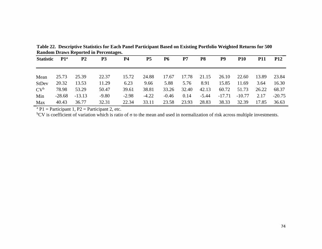
74
Table 22. Descriptive Statistics for Each Panel Participant Based on Existing Portfolio Weighted Returns for 500
Random Draws Reported in Percentages.
Statistic P1a P2 P3 P4 P5 P6 P7 P8 P9 P10 P11 P12
Mean 25.73 25.39 22.37 15.72 24.88 17.67 17.78 21.15 26.10 22.60 13.89 23.84
StDev 20.32 13.53 11.29 6.23 9.66 5.88 5.76 8.91 15.85 11.69 3.64 16.30
CVb 78.98 53.29 50.47 39.61 38.81 33.26 32.40 42.13 60.72 51.73 26.22 68.37
Min -28.68 -13.13 -9.80 -2.98 -4.22 -0.46 0.14 -5.44 -17.71 -10.77 2.17 -20.75
Max 40.43 36.77 32.31 22.34 33.11 23.58 23.93 28.83 38.33 32.39 17.85 36.63 a P1 = Participant 1, P2 = Participant 2, etc. bCV is coefficient of variation which is ratio of σ to the mean and used in normalization of risk across multiple investments.

75
75
Table 23. Descriptive Statistics for Portfolio Strategies for Returns Weighted
According to the Nonlinear Programming Analysis. Based on 500 Random
Draws and Reported in Percentages.
Statistic PURa P2D PSM PE PMD
Mean 6.04 10.34 9.64 40.90 15.51
StDev 0.63 0.92 0.81 19.18 4.93
CV 10.41 8.90 8.44 46.89 31.75
Min 4.74 6.29 7.32 -13.77 -6.81
Max 7.65 12.04 11.58 56.41 20.35
a PUR = no restrictions on amount of portfolio in each investment option. P2D =
total investment in each option limited by resources available. PSM = total
investment in each option constrained to be no larger than the largest percentage
invested by an individual member of the panel in that option. PE = investments
constrained to be equal across all investment options. PMD = investments
constrained to be no more than 20 percent of total portfolio in any single investment
option.
76
76
on the frequent assumption that agricultural producers are risk-averse. The results
reported in Table 24 suggest that risk-averse producers tend not to prefer cattle as
their largest single investment. This is true given that the four most preferred actual
portfolios for risk-seeking participants (P1, P9, P12, and P2) also have the largest
proportions of their investments in cattle of the 12 Panel participants. This suggests
that participants with relatively large investments in cattle tend to prefer more risk
than those with larger investments in camels and other “safer” forms of investment.
The four preferred portfolios for risk-averse decision makers (P7, P6, P11, and P5)
focus on investing in camels and other relatively safe investments such as real estate,
but cattle also remain a significant part of the investment portfolio (average
proportion of portfolio for P7, P6, P11, and P5 is slightly less than 23 percent). Cattle
offer a positive and relatively large return in eight out of 10 years based on their
empirical cdf (Table 18). So, they appear to remain an important part of the
investment mix for risk-averse producers. This may also reflect the complementarity
of camels and cattle in the grazing system where cattle primarily eat grass and camels
primarily eat browse. As a result, having both species results in utilization of a
broader spectrum of rangeland feed than one of the species alone (Forrest et al 2015).
The dominant risk-averse strategies (P7, P6, P11, and P5) support the notion
that the Panel participants follow a risk-spreading investment strategy. This suggests
that the most risk-averse Panel participants still see benefit in investment in relatively

77
77
Table 24. Efficient Sets for Risk Adverse Decision Makers Identified by the
Stochastic Dominance Analysis.
Efficient Set for Efficient Set for Hypothetical
Actual Portfoliosa Portfolios Identified by NLPb
P7 Most Preferred
P6 2nd Most Preferred
P11 3rd Most Preferred
P5 4th Most Preferred
P4 5th Most Preferred
P8 6th Most Preferred
P3 7th Most Preferred
P10 8th Most Preferred
P2 9th Most Preferred
P9 10th Most Preferred
P12 11th Most Preferred
P1 12th Most Preferred
P2D Most Preferred
PSM 2nd Most Preferred
PMD 3rd Most Preferred
PUR 4th Most Preferred
PE Least Preferred
a See Table 14 for portfolios of individual Panel participants. b See footnotes to Table 15 for description of the NLP Portfolio constrains. Table 17
provides information on the portfolio determined for each of these strategies. c P1 = portfolio actually help by Participant 1, etc.

78
78
risky assets such as cattle as being an important component of the overall investment
strategy. However, cattle are clearly not preferred to camels by risk-averse decision
makers.
This finding is potentially important. It suggest that the current environment
relating to livestock production risks on the Borana Plateau favors a continued move
to more camels and fewer cattle. However, there may be constraints on how much
more the camel population can expand. Forrest et al. (2015) suggest that camels
alone are unable to support the human population on the Borana Plateau. These
results suggest that incentives exist for risk-averse pastoralists to continue to move
away from cattle and toward more camels. This trend is likely to continue without
drought mitigation strategies that support cattle grazing, such as bush clearing
(Forrest et al. 2015).
As was generally expected, the NLP strategies that are preferred by risk-
averse decision makers favored minimizing the variance of returns such as was done
in P2D, PSM, and PMD (Table 24) rather than diversification across investment
options (PE, PUR). Clearly these pastoralists understand the tradeoffs exist between
expected average returns and risks because they appear to follow primarily risk-
spreading diversification strategies (Table 14). They are willing to accept some
additional risk if the expected payoffs are high enough. This is exhibited by the fact
that P2D, PSM, and PMD avoided placing cattle in the portfolio in favor of camels
(Table 24). This departs from the strategy actually followed by the Panel

79
79
participants, but supports the pressure for more camels to reduce risk as indicated by
the most efficient sets identified for risk-averse decision makers (Table 24).
Results of the Stochastic Efficiency Analysis
The SERF analysis closely reflects the one provided by the stochastic
dominance analysis. Figure 3 shows that the actual portfolio held by P1 is the most
preferred portfolio for risk-seeking decision makers. Table 25 reports the inputted
risk premiums that are implied by the results depicted in Figure 3. The analysis
demonstrates that the efficient set for the different portfolios remains constant at all
levels for a risk-seeking decision maker. Figure 4 and Table 26 present the SERF
analysis and implied risk premium, respectively, for the five portfolio selected by the
NLP.30
While the SERF results are important visually, they offer little new
information not contained in the stochastic dominance analysis. In either case,
pastoralists will prefer to place most of their assets in livestock, particularly cattle and
secondarily camels, and then diversity into one or two less risky investment options.
The results presented by Forrest et al. (2015) demonstrated the importance of cattle to
the livestock, and indeed, the economic system existing on the Borana Plateau. This
analysis also demonstrates the critical central role that cattle play in this system not
only in providing food consumption products (primarily milk), but also as a critical
part of the risk management strategies pursued by pastoralists. As was suggested in
30 For purposes of comparison, see rankings of portfolios by E-V in Tables 27 and 28.

80
80
Figure 3. SERF chart depicting risk premiums for different actual portfolios
based on risk preference.
P1P2P3
P4
P5
P6P7
P8
P9
P10
P11
P12
-20.00
-10.00
0.00
10.00
20.00
30.00
40.00
-0.3 -0.2 -0.1 0 0.1 0.2 0.3Ce
rtai
nty
Eq
uiv
ale
nt
ARAC
Stochastic Efficiency with Respect to A Function (SERF) Under a Neg. Exponential
Utility Function
P1 P2 P3 P4 P5 P6
P7 P8 P9 P10 P11 P12

81
Table 25. Implied Risk Premiums for Actual Portfolios Compared to the Actual Portfolio Held by P1 Based on Risk
Preferences.
Statistic P1a P2 P3 P4 P5 P6 P7 P8 P9 P10 P11 P12
Mean - 4.55 2.91 (1.30) 6.30 0.75 0.90 2.97 3.62 2.87 (2.49) 1.10
StDev - 9.32 12.19 17.65 14.09 17.94 18.04 14.96 6.23 11.69 19.48 5.65
a P1 = Participant 1, P2 = Participant 2, etc.

82
Figure 4. SERF chart depicting risk premiums for different NLP portfolios
based on risk preference.
PURP2DPSM
PE
PMD
0.00
10.00
20.00
30.00
40.00
50.00
60.00
-0.4 -0.3 -0.2 -0.1 0 0.1 0.2 0.3 0.4
Ce
rtai
nty
Eq
uiv
ale
nt
ARAC
Stochastic Efficiency with Respect to A Function (SERF) Under a Neg. Exponential
Utility Function
PUR P2D PSM PE PMD

83
Table 26. Implied Risk Premiums for Actual Portfolios Compared to PUR
Based on Risk Preferences.
Statistic PURa P2D PSM PE PMD
Mean - 1.3 3.6 26 8.66
StDev - 0.04 0.02 19.6 2.5
a PUR = no restrictions on amount of portfolio in each investment option. P2D =
total investment in each option limited by resources available. PSM = total
investment in each option constrained to be no larger than the largest percentage
invested by an individual member of the panel in that option. PE = investments
constrained to be equal across all investment options. PMD = investments
constrained to be no more than 20 percent of total portfolio in any single investment
option.
Table 27. Ranking of 12 Panel Participants Using Mean Return and CV.
Participanta Mean Return CV
Value Rankb Value Rankc
P1 25.73 2 78.98 12
P2 25.39 3 53.29 9
P3 22.37 7 50.47 7
P4 15.72 11 39.61 5
P5 24.88 4 38.81 4
P6 17.67 10 33.26 3
P7 17.78 9 32.40 2
P8 21.15 8 42.13 6
P9 26.10 1 60.72 10
P10 22.60 6 51.73 8
P11 13.89 12 26.22 1
P12 23.84 5 68.37 11 a P1 = Participant 1, P2 = Participant 2, etc. b The mean returns are ranked with 1 being the participant with the highest return and
12 is the participant with the lowest return.
c CV is ranked with 1 being the participant with the lowest risk and 12 is the
participant with the highest risk.

84
Table 28. Ranking of Five NLP Portfolios by Mean Return and CV.
Modela
Mean
Return CV
Value Rankb Value Rankc
PUR 6.04 5 10.41 3
P2D 10.34 3 8.90 2
PSM 9.64 4 8.44 1
PE 40.90 1 46.89 5
PMD 15.51 2 31.75 4 a PUR = no restrictions on amount of portfolio in each investment option. P2D =
total investment in each option limited by resources available. PSM = total
investment in each option constrained to be no larger than the largest percentage
invested by an individual member of the panel in that option. PE = investments
constrained to be equal across all investment options. PMD = investments
constrained to be no more than 20 percent of total portfolio in any single investment
option. b The mean returns are ranked with 1 being the portfolio with the highest return and 5
is the portfolio with the lowest return.
c CV is ranked with 1 being the portfolio with the lowest risk and 5 is the portfolio
with the highest risk.
85
Forrest et al., camels can play a role in risk management in the Borana Plateau, but
this role is expected to remain a secondary one to cattle in this system.
The results also suggest that efforts that have been made to encourage
pastoralists to diversify into non-agricultural assets such as bank accounts and real
estate (Desta 1999) are well founded. However, these alternative investments should
be seen as complementary to livestock production, especially cattle production.

86
CHAPTER 5
DISCUSSION AND CONCLUSIONS
The need for securing more food resources as the world population increases
has become a main concern for governments and NGOs around the world especially
in planning future sustainable polices and aid projects. Sub-Saharan African
countries and especially Ethiopia have been a focus of many aid projects for many
years. Livestock production has been an important economic and social livelihood
activity in this region.
Pastoralism in Ethiopia and on the Borana Plateau in the south has been a way
of life for many generations. Many factors such as droughts and degradation and
reduction of rangeland because of the increasing human and livestock population
affected the livelihood of pastoralists in this region.
There has been a need for better risk management strategies for pastoralists in
this region to diversify their investment portfolio. It is important to understand the
nature of risk for pastoralist investment portfolios and how pastoralists perceive risk
when making investment choices. The purpose of study was to provide insights
toward understanding investment opportunities, choices, and the risk pastoralists are
facing. The data were collected from field interviews of 12 influential and wealthy
pastoralists in the Yabelo District of the Borana Plateau. The wealthy pastoralist’s
Panel was chosen because the relatively large amount of discretionary income they

87
can invest compared to most people in the Borana Plateau and their large-sized herds
which consume more water and forage resources than the small herds owned by the
rest of the community. Wealthy pastoralists also provide employment for local
communities through milking and herding their livestock.
The main investment options that members of the panel are currently
investing are divided in to livestock sector (cattle, camels, sheep and goats),
nonagricultural sector investments (bank saving accounts and real estate) and
cropping represented here by maize and haricot beans. The returns on those
investments were calculated using a return on assets (ROA) approach based on the
responses to a survey questionnaire provided to the Panel and secondary data taken
from previous research. Average returns for the investment options were
estimated/calculated over a 10-year period assuming the first four years were normal-
rainfall years with livestock herds at full capacity followed by two years of drought
and then four herd rebuilding years with normal rainfall.
The analytical methods used in this thesis used the rates of return on the
different types of investments, risk associated with those returns and risk bearing
preferences for different decisions makers. Nonlinear programming analysis was
used to create optimum portfolios based on the assumption that decision makers
minimize risk at every given rate of return through the selection of investment
alternatives that do so. Stochastic dominance analysis was used to determine the
most efficient investment when compared to one another, and stochastic efficiency
analysis was used to compare investment strategies to identify whether the investment
88
strategies being pursued by the Panel participants reflected risk-averse or risk –
seeking behaviors.
The 12 panel members are entrepreneurs who have limited education and who
worked hard from a young age to grow their herds. Identifying opportunities and
ways to measure the importance of education in helping and supporting pastoralists
make appropriate investments would be a good contribution to the literature, but is
not tested in this study. Some of the Panel members inherited the herds and others
started their own .They all had to suffer through local conflicts and natural disasters
like droughts and they lost large numbers of their herds during this hard time. The
age of the Panel members ranged from 50 to 98 years old. They accumulated their
livestock herds to provide meat and milk needs for their families, as a source of
income and as a source of social feeling of security.
The Panel participants appear to understand the tradeoffs between expected
average returns and risk because they clearly pursue building diversified portfolios
that have larger than expected rates of return and larger variances than simply putting
their money into bank savings accounts (essentially a guaranteed investment). The
Panel participants still invest heavily livestock investments (cattle, camel, goat and
sheep) instead of evenly distributing their portfolio among the different investments.
However, very risk-averse Panel members tend to invest more in camels than in
cattle. As a result, risk-averse producers tend to avoid cattle as their largest single
investment comparing with the risk seeking producers who invested large proportions
of their portfolios in cattle. Risk-averse producers also tended to combine livestock
89
investments (especially camels) with safer investments options such as saving bank
accounts and real estate. Cattle remain an important part of the overall investment
strategy even with risk-averse producers.
Risk-averse producers favor camels over cattle and this suggests that the
current environment in the Borana plateau favors a continued moves towards camels
instead of cattle. The results also support the efforts that have been made to
encourage pastoralist to diversify into alternative investments such as non-agriculture
assets (real estate and saving accounts). More research is needed for a better
understanding of how to determine how much the camel population can increased
while side-by-side with cattle to support the human population during droughts.
The results from this study closely match the current perception of the 12
Panel participants. They ranked the risk associated with cattle as the highest and for
camels as the lowest for investments in livestock. They also ranked livestock
investment with regard to the perceived risk of investments as the highest compared
to savings accounts and real estate. This also supports the movement toward less
investment in cattle and more investment in other alternatives.
The results are consistent with the notion that more diversification results in
lower risks for pastoralists, or at least provides an avenue for reducing risks if
pastoralists choose to use them. This conclusion matches that of Desta (1999) who
suggested that the best investment portfolio option for pastoralists was combining
cattle with safe banking. The results reported here also support the idea that bank
accounts can reduce pastoralists’ risk. However, other relatively safe investments,

90
such as real estate or camels, offer higher returns than saving accounts for pastoralists
seeking to reduce their risks.

91
REFERENCES
Access Capital Research. May 2010. Sector Report—Real Estate. Available online at
http://www.ethioconstruction.net/sites/default/files/Law/Files/Sector%20Repo
rt--Real%20Estate.pdf.
Africa and Ethiopia Map. Available online at http://www.nationmaster.com/country-
info/profiles/Ethiopia
Barrett, Christopher B., Thomas Reardon, and Patrick Webb. 2001. "Nonfarm income
diversification and household livelihood strategies in rural Africa: concepts,
dynamics, and policy implications." Food policy 26, no. 4: 315-331.
Beddington, John. 2009. "Food, energy, water and the climate: a perfect storm of
global events." In Lecture to Sustainable Development UK 09 Conference,
vol. 19..
Bekele, Eshetu, and Zeleke Worku. 2008. "Factors that affect the long‐term survival
of micro, small and medium enterprises in Ethiopia." South African Journal of
Economics 76, no. 3: 548-568.
Berhanu, Wassie, David Colman, and Bichaka Fayissa. 2007. "Diversification and
livelihood sustainability in a semi-arid environment: A case study from
southern Ethiopia." Journal of Development Studies 43, no. 5: 871-889.
Bourguignon, François, and Christian Morrisson. "Inequality among world citizens:
1820-1992." American economic review (2002): 727-744.
Borana Plateau map. Available online at
https://www.google.com/maps/@8.1789002,39.0964242,6z
Bradley, Stephen P., Arnoldo C. Hax, and Thomas L. Magnanti. “Applied
mathematical programming”. Reading, MA: Addison-Wesley, 1977.
Bruinsma, Jelle. 2003. “World agriculture: towards 2015/2030. An FAO
perspective”. Earthscan Publications Ltd,.
Commercial Bank of Ethiopia. 2015. Found online at
http://www.combanketh.et/DomesticBanking/Deposits/SavingsAccount.aspx.
Coppock, D. L., G. Gebru, S. Mesele, and S. Desta. 2008. “Are Drought-Related
Crashes in Pastoral Cattle Herds Predictable? More Evidence of Equilibrium
Dynamics from Southern Ethiopian Rangelands.” Page 1090 in
Multifunctional Grasslands in a Changing World, volume II, Edited by the

92
Organizing Committee of the 2008 International Grasslands
Congress/International Rangelands Congress (IGC/IRC). Guagdong People’s
Publishing House, Beijing. pp. 1,154.
Coppock, David Layne, ed. 1994. The Borana Plateau of Southern Ethiopia:
Synthesis of pastoral research, development, and change, 1980-91. No. 5.
ILRI (aka ILCA and ILRAD).
Coppock, David Layne, Getachew Gebru, Solomon Desta, Sintayehu Mesele, and
Seyoum Tezerra. 2008."Are Cattle Die-Offs Predictable on the Borana
Plateau?".
Coppock, David Layne, Seyoum Tezera, Bedasa Eba, Jaldessa Doyo, Demisachew
Tadele, Derege Teshome, Nizam Husein, and Meiso Guru. 2014."Sustainable
Pastoralism on the Borana Plateau: An Innovation Systems Approach.".
Davies, James B., Anthony Shorrocks, Susanna Sandstrom, and Edward N. Wolff.
2007. "The world distribution of household wealth." Center for Global,
International and Regional Studies.
Davies, James B., Anthony Shorrocks, Susanna Sandstrom, and Edward N. Wolff.
2007. "The world distribution of household wealth." Center for Global,
International and Regional Studies .
Department of State: 2014 Investment Climate Statement Ethiopia June 2014 Cheryl
Monticello, Commercial Officer, [email protected], 011 130 6588.
Abdulkader Hussen, Commercial Specialist, [email protected], 011 130
6177.U.S. Embassy, PO Box 1014, Addis Ababa Ethiopia.
Dercon, Stefan. 2002. "Income risk, coping strategies, and safety nets." The World
Bank Research Observer 17, no. 2: 141-166.
Desta, S. and D. L. Coppock.2002. “Cattle Population Dynamics in the Southern
Ethiopian Rangelands, 1980-97.” Journal of Range Management, 55: 439-
451.
Desta, Solomon, and D. Layne Coppock. 2002. "Cattle population dynamics in the
southern Ethiopian rangelands, 1980-97." Journal of Range Management:
439-451.
Desta, Solomon. 1999. "Diversification of livestock assets for risk management in the
Borana pastoral system of southern Ethiopia." PhD diss., Utah State
University. Department of Rangeland Resources.
93
Ellis, Frank. 1998. "Household strategies and rural livelihood diversification." The
journal of development studies 35, no. 1: 1-38.
Ellis, Frank. 1999. “Rural livelihood diversity in developing countries: evidence and
policy implications.” London: Overseas Development Institute.
Embassy of The Federal Democratic Republic of Ethiopia investment opportunities
2014
Ethiopia Interest Rate 2003-2012. Available online at
http://www.tradingeconomics.com/ethiopia/interest-rate.
Ethiopia Rural Socioeconomic Survey. May 7th, 2013. (ERSS) Survey Report.
Central Statistical Agency & the World Bank.
Ethiopian Ministry of Agriculture, 2015, land lease information. Found online at
http://www.moa.gov.et/land-leased.
Ethiopian Road Authority. 2009. Revised Universal Rural Road Access Program,
Addis Ababa.
FAO. 2013. Ethiopia overview
http://www.fao.org/countryprofiles/index/en/?iso3=eth.
FAO, 2009 How to feed the world in 2050 report (FAO). Found online at :
http://www.fao.org/fileadmin/templates/wsfs/docs/expert_paper/How_to_Feed
_the_World_in_2050.pdf
FAO, IFAD and WFP. 2014. The State of Food Insecurity in the World 2014.
Strengthening the enabling environment for food security and nutrition.
Rome, FAO. Found online at http://www.fao.org/3/a-i4030e.pdf
Federal Ministry of Education, August 2010. Addis Ababa, Ethiopia, Education
Sector Development Program IV (ESDP IV) 2010/2011 – 2014/2015.
Program Action Plan.
FIAN G8 Cooperation framework to support The “G8 new alliance for food security
and nutrition in Africa” Editors: Editors: Roman Herre, Philip Seufert, Yifang
Slot-Tang, Denisse Cordova, Flavio Valente, Laura Michéle. February 21014
.Available online at
http://www.fian.org/fileadmin/media/publications/2014_G8NewAlliance_scre
en.pdf
Forrest, B. 2014. “Analysis of Building Resiliency in an Ethiopian Pastoral System:
Mitigating the Effect of Population and Climate Change on Food Insecurity”.

94
MS thesis. Department of Applied Economics, Utah State University, Logan,
Utah.
Forrest, Brigham W., D. Layne Coppock, DeeVon Bailey, and Ruby A.
Ward. February 2015. “Economic
Analysis of Land and Livestock Management Interventions to Improve
Resiliency of a Pastoral Community in Southern Ethiopia.” Journal paper
8670, Utah Agricultural Experiment Station and Department of Applied
Economics, Utah State University, Logan, Utah.
Funk, Chris, Jim Rowland, Gary Eilerts, Emebet Kebebe, Nigist Biru, Libby White,
and Gideon Galu. 2012. "A climate trend analysis of Ethiopia." US Geological
Survey, Fact Sheet 3053.
Gemtessa, Kejela, Bezabih Emana, and Waktole Tiki. 2005."Livelihood
Diversification in Borana: Pastoral Communities of Ethiopia–Prospects and
Challenges." Unpublished report by WABEKBON Consult, Ethiopia .
Getachew, Dereje, and Tesfatsion Sahlu. 2013."Determinants of Trade Credit Use by
Private Traders in Ethiopia: Case of Mekelle City, Tigray Regional State.”
Research Journal of Finance and Accounting 4, no. 10: 1-7.
Hadar, Josef, and William R. Russell. 1969. "Rules for ordering uncertain
prospects.” The American Economic Review: 25-34.
Hammond, Geoffrey P. 2000. "Energy, environment and sustainable development: a
UK perspective." Process Safety and Environmental Protection 78, no. 4:
304-323.
Hardaker, J. Brian, James W. Richardson, Gudbrand Lien, and Keith D. Schumann.
2004. "Stochastic efficiency analysis with risk aversion bounds: a simplified
approach." Australian Journal of Agricultural and Resource Economics 48,
no. 2 (2004): 253-270.
Hazell, Peter BR, and Roger D. Norton. 1986. “Mathematical programming for
economic analysis in agriculture.” New York: Macmillan.
Helmberger, Peter G., Jean-Paul Chavas. 1996. The Economics of Agricultural
Prices. Prentice Hall: Upper Saddle River, NJ. .
Hogg, Richard. 1996. "Government policy and pastoralism: Some critical issues." In
Conference on pastoralism in Ethiopia: Full papers.

95
Ionescu, Luminiţa. 2011. "The financial crisis as a failure of corporate
governance."Economics, Management, and Financial Markets 2: 827-832.
Investing in smallholder family farmers for the future we want International Fund for
Agricultural Development. 2014. Governing council .Via Paolo di Dono, 44 -
00142 Rome, Italy.
Kaufmann, B. 1998 “Analysis of Pastoral Camel Husbandry in Northern Kenya.”
Weikersheim, Germany:Margraf Verlag.
Lavers, Tom. 2013. "The role of foreign investment in Ethiopia’s smallholder
agricultural development strategy.".
Leamer, Edward E. 2007.“Housing is the business cycle.” No. w13428. National
Bureau of Economic Research.
Lintner, John. 1965. "The valuation of risk assets and the selection of risky
investments in stock portfolios and capital budgets." The review of economics
and statistics: 13-37.
Little, Peter D., Kevin Smith, Barbara A. Cellarius, D. Layne Coppock, and
Christopher Barrett. 2001. "Avoiding disaster: diversification and risk
management among East African herders." Development and Change 32, no.
3: 401-433.
Little, Peter. 2009. "Hidden value on the hoof: cross-border livestock trade in Eastern
Africa." Policy Brief 2.
Loening, Josef, and Laketch Mikael Imru. "Ethiopia: diversifying the rural economy.
An assessment of the investment climate for small and informal enterprises."
Lybbert, Travis, Christopher Barrett, Solomon Desta, and D. Layne Coppock. 2009.
"Pastoral risk and wealth-differentiated herd accumulation in southern
Ethiopia." USAID, Utah State University, International Livestock Research
Institute, and the Rockefeller Foundation (2001).
Manos, Basil D., and George I. Kitsopanidis. 1986. "A quadratic programming model
for farm planning of a region in central Macedonia." Interfaces 16, no. 4: 2-
12.
Mapp, Harry P., Michael L. Hardin, Odell L. Walker, and Tillak Persaud. 1979
"Analysis of risk management strategies for agricultural
producers." American Journal of Agricultural Economics: 1071-1077.

96
Markowitz, Harry. "Portfolio selection." The journal of finance 7, no. 1 (1952): 77-
91.
McCarl, Bruce A., and David A. Bessler. 1989. "Estimating an upper bound on the
pratt risk aversion coefficient when the utility function is
unknown*." Australian Journal of Agricultural Economics 33, no. 1: 56-63.
McPeak, John G., and Christopher B. Barrett. 2001. "Differential risk exposure and
stochastic poverty traps among East African pastoralists." American Journal
of Agricultural Economics: 674-679.
McPeak, John G., and Peter D. Little. 2006 “Pastoral livestock marketing in Eastern
Africa: research and policy challenges.” Intermediate Technology
Publications Ltd.
McPeak, John G., Peter D. Little, and Cheryl R. Doss. 2011. “Risk and social change
in an African rural economy: livelihoods in pastoralist communities.” Vol. 7.
Routledge.
Mengesha, Teferra. 23 – 25 November 2010.“Emancipating the Rural Population
from Isolation. Intermediate Means of Transport (IMTs) The Case of Ethiopia
in Sub-Saharan Africa.” A Paper Presenting at the 1st AFCAP Practitioners
Conference.. Addis Ababa.. W.T Consult PLC.
Merton, Robert C. 1977"On the microeconomic theory of investment under
uncertainty.”
Meyer, Jack. 1977a. "Choice among distributions." Journal of Economic Theory 14,
no. 2: 326-336.
Meyer, Jack. 1977b "Second degree stochastic dominance with respect to a
function." International Economic Review: 477-487.
Milanovic, Branko. 2005 "Worlds apart." Measuring International and Global
Inequality, Princeton and Oxford: Princeton University Press, 227p .
Moss, Charles B. October 5, 2010. “Utility Functions, Risk Aversion Coefficients
and Transformations:
Lecture XVIII.” Available online at
http://ricardo.ifas.ufl.edu/aeb6182.risk/Slides18-2010.pdf.
2015.
Mude, Andrew, Christopher B. Barrett, Michael R. Carter, Sommarat Chantarat,
Munenobu Ikegami, and John G. McPeak. 2009"Index based livestock

97
insurance for northern Kenya’s arid and semi-arid lands: the Marsabit pilot."
SSRN 1844758.
Norstad, John. 1999. "An introduction to utility theory." Unpublished manuscript at
http://homepage. mac. com/j. norstad .
Peden, D., A. Freeman, A. Astatke, A. Notenbaert, W. Ayalneh, and I. Baltenweck.
2006. "Investment options for integrated water-livestock-crop production in
sub-Saharan Africa." ILRI Work. Pap ).
Privatization and the Public Enterprises Supervising Authority (PPESA). Available
online at http://www.ppesa.gov.et/.
Randers, Jorgen. 2008. "Global collapse—Fact or fiction? " Futures 40, no. 10: 853-
864
Richardson, James W. 2006. "Simulation for applied risk management." Department
of Agricultural Economics, Agricultural and Food policy center, Texas A&M
University.
Runge, C. Ford, Benjamin Senauer, Philip G. Pardey, and Mark W. Rosegrant. 2003.
Ending hunger in our lifetime: food security and globalization. Intl Food
Policy Res Inst,.
Sharpe, William F. 1964. "Capital asset prices: A theory of market equilibrium under
conditions of risk*." The journal of finance 19, no. 3: 425-442.
Swallow, Brent M. 1994 “The role of mobility within the risk management strategies
of pastoralists and agro-pastoralists.” London: International Institute for
Environment and Development.
Swift, Jeremy, Kate Hamilton, S. Devereux, and S. Maxwell. 2001 "Household food
and livelihood security." Food security in sub-saharan Africa : 67-92.
Tache, Boku, and Gufu Oba. 2010. "Is poverty driving Borana herders in Southern
Ethiopia to crop cultivation?" Human ecology 38, no. 5: 639-649.
The state of food insecurity in the world, the multiple dimensions of food security
report 2013. FAO Population Division of the Department of Economic and
Social Affairs of the United Nations Secretariat 2011. World Population
Prospects: The 2008 Revision, http://esa.un.org/unpp
Tobin, James. 1958"Liquidity preference as behavior towards risk." The review of
economic studies: 65-86.
98
Tomek, William G., and Hikaru Hanawa Peterson. 2001."Risk management in
agricultural markets: a review." Journal of Futures Markets 21, no. 10: 953-
985.
UNCTAD, World Investment Report 2014” Investing In the SDGS: An Action Plan”.
United Nations Publication Sales No. E.14.II.D.1 ISBN 978-92-1-112873-4
eISBN 978-92-1-056696-4
United Nations Millennium Development Goals (MDGs), fact sheet (1).
“n.d.”Available online at
http://www.un.org/millenniumgoals/pdf/Goal_1_fs.pdf.
USAID, Ethiopia, Country Development Cooperation Strategy 2011 – 2015
Accelerating the Transformation toward Prosperity PUBLIC VERSION:
March 2012.
USTR, Office the United States trade representative, Executive office of the
president, Ethiopia report 2013
http://www.ustr.gov/sites/default/files/Ethiopia_0.pdf.
Valadez, Ray M. 2010."The housing bubble and the GDP: a correlation perspective.
“Journal of Case Research in Business & Economics 3: 1-18.
Von Braun, Joachim. 2005. The world food situation: an overview. International food
policy research institute (IFPRI).
World Bank, 2014, Africa’s Pulse An analysis of issues shaping Africa’s economic
future April 2014 volume 9. Found online at
http://www.worldbank.org/content/dam/Worldbank/document/Africa/Report/
Africas-Pulse-brochure_Vol9.pdf.
Weisstein, Eric W. “Distribution Function." From MathWorld--A Wolfram Web
Resource. http://mathworld.wolfram.com/DistributionFunction.html
World Bank data base Ethiopia overview. “n.d.” Available online at
http://www.worldbank.org/en/country/ethiopia/overview.
World Bank, databank,
http://databank.worldbank.org/data/views/reports/tableview.aspx.
World Bank. 2010. Ethiopia - Protecting the most vulnerable. IDA at work.
Washington, DC: World Bank Group. Available online at

99
http://documents.worldbank.org/curated/en/2010/09/20372040/ethiopia-
protecting-most-vulnerable.
World Bank. 2012. Agribusiness indicators - Ethiopia. Washington, DC: World Bank.
Available online at
http://documents.worldbank.org/curated/en/2012/04/16374742/agribusiness-
indicators-ethiopia.
World Bank. 2013. Ethiopia - Second Phase of General Education Quality
Improvement Project. Washington DC; World Bank. Available online
athttp://documents.worldbank.org/curated/en/2013/10/18499496/ethiopia-
second-phase-general-education-quality-improvement-project.
WTO, World Trade Organization, 2012, found online at
http://stat.wto.org/TariffProfiles/ET_e.htm
Zuberi, Tukufu, and Kevin JA Thomas. 2012. Demographic projections, the
environment and food security in Sub-Saharan Africa. No. 2012-001.
Zeru, Fetene. 2010. “Access to Finance and Its Challenge for Small Business
Enterprises.” Case of Addis Ababa City Study conducted in partial fulfilment
of the MSc in accounting and finance. Submitted to Addis Ababa University,
School of Business and Public Administration, Department of Accounting and
Finance.

100
APPENDIX

101
Survey questions
PASTORAL WEALTH AND ALTERNATIVE INVESTMENT INTERVIEW
1. You have been selected for this interview because you are regarded as an
important member of the Borana community who has great wealth. Please
describe your life since you were a young boy. What are the most important
reasons why you have become so wealthy and successful?
2. How old are you now? Where do you live? How long have you lived in the
Borana region?
3. How many wives and children have you had? Where do your wives and
children live?
4. Have any of your children received formal or informal education? If “yes”
list them by name, the level completed and what they are doing now. Expand
table if needed (if “no,” skip to #5).
ID
Number
Gender Formal
Level?
Informal
Level?
What is the child’s age, and
what is he/she doing now?
5. Have any of your wives received formal or informal education? If “yes,” list
them by name, the level completed, and what they are doing now. Expand
table if needed. (If “no,” skip to #6).
ID Number Formal
Level?
Informal
Level?
What is the wife doing now?

102
6. Have you ever received formal or informal education? If “yes,” please
specify formal or informal and indicate level(s) completed. (If “no,” note
below and skip to the next question.)
7. Can you read or write? If “yes,” please specify the level for each. If “no,” is
this a problem for you? Please explain.
8. You are known for having large numbers of livestock. Why do you want to
accumulate large numbers of livestock? (multiple reasons are fine – try to
rank in terms of importance.)
9. Do you own different species of livestock? (Examples: cattle, camels, sheep,
goats, horses, donkeys, mules). Answer “yes” or “no.”
10. If you own more than one species of livestock, explain why. In other words,
what are the advantages and disadvantages for each species?
11. What are the specific benefits to you of having large numbers of livestock?
12. What are the specific problems for you when having large numbers of
livestock?
13. Who did the herding and milking work for your animals 15 years ago?
14. Who does the herding and milking work for your animals today?
15. If there has been a change in the types of people who contribute labor for your
herds over the past 15 years, explain why. If there has been no change, also
explain why.
16. In Borana culture, the wealthy herd owners used to give milk and calves to the
poor people in return for the labor of the poor people who herded and milked
animals owned by the wealthy. This process could help the poor re-build their
herds over time. Did you or your father engage in this practice years ago—yes
or no? Do you engage in this practice today—yes or no? If this practice has
changed, please explain when it began to change, and why.
17. What is your opinion of poor people in Borana today? Why do you think they
are poor? Are they able today to build-up their herds to become wealthy, or not?
103
18. Besides livestock, do you own any of the following?
(a) Huts (where people live in an olla)
i. Number and locations
(b) Houses (where people can live)
i. Number, locations, sizes, values in Birr (and specify partial
ownership)
(c) Small shop (duka; market outlet), butchery, tea shop, etc.
i. Number, locations, sizes, values in Birr (and specify partial
ownership)
(d) Hotels
i. Number, locations, sizes, values in Birr (and specify partial
ownership)
(e) Other roofed buildings (storage facilities, slaughter facilities, etc.)
i. Number, locations, sizes, values in Birr (and specify partial
ownership)
(f) Livestock holding-grounds or feedlots
i. Number, locations, sizes, values in Birr (and specify partial
ownership)
(g) Motor vehicles (lorries, cars, buses, motorcycles)
i. Type, number, locations, value in Birr (and specify partial ownership)
(h) Other physical assets not yet mentioned
i. Type, number, locations, value in Birr (and specify partial ownership)
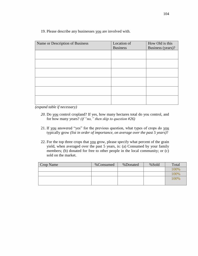
104
19. Please describe any businesses you are involved with.
Name or Description of Business Location of
Business
How Old is this
Business (years)?
(expand table if necessary)
20. Do you control cropland? If yes, how many hectares total do you control, and
for how many years? (if “no,” then skip to question #26)
21. If you answered “yes” for the previous question, what types of crops do you
typically grow (list in order of importance, on average over the past 5 years)?
22. For the top three crops that you grow, please specify what percent of the grain
yield, when averaged over the past 5 years, is: (a) Consumed by your family
members; (b) donated for free to other people in the local community; or (c)
sold on the market.
Crop Name %Consumed %Donated %Sold Total
100%
100%
100%

105
23. For the same three crops, please note the frequency of crop failures when little
or no grain is produced.
Crop Name Fails 1
in 2
years
1 in 3
years
1 in 4
years
1 in 5
years
1 in 7
years
1 in 8
years
1 in 9
years
1 in 10
years
Other
(years)
24. Do you also use your cropland (or fenced cropland area) for kalo? If “yes,” give
the size (hectares) for each kalo in the cropland areas you control, and note if
the grazing use is “private” (for your animals only) or if it is open to the
community. (If “no,” skip to question #26) Expand table if necessary.
Kalo name (or
other identifier)
Kalo size
(hectares)
Private Use
Only?
Mixed Private and
Community Use?
Community Use
Only?
Leased to
Traders or
Others?
25. Briefly explain how and when the kalo in question #24 are used.
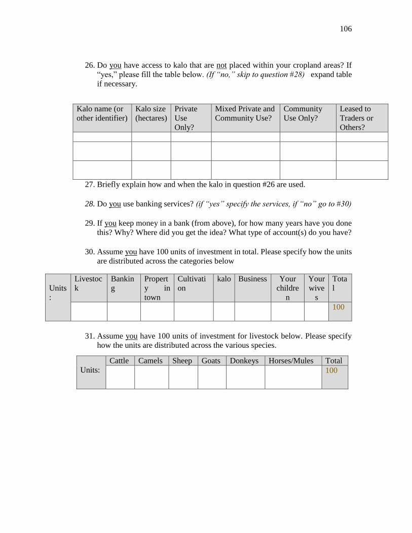
106
26. Do you have access to kalo that are not placed within your cropland areas? If
“yes,” please fill the table below. (If “no,” skip to question #28) expand table
if necessary.
Kalo name (or
other identifier)
Kalo size
(hectares)
Private
Use
Only?
Mixed Private and
Community Use?
Community
Use Only?
Leased to
Traders or
Others?
27. Briefly explain how and when the kalo in question #26 are used.
28. Do you use banking services? (if “yes” specify the services, if “no” go to #30)
29. If you keep money in a bank (from above), for how many years have you done
this? Why? Where did you get the idea? What type of account(s) do you have?
30. Assume you have 100 units of investment in total. Please specify how the units
are distributed across the categories below
31. Assume you have 100 units of investment for livestock below. Please specify
how the units are distributed across the various species.
Units
:
Livestoc
k
Bankin
g
Propert
y in
town
Cultivati
on
kalo Business Your
childre
n
Your
wive
s
Tota
l
100
Units:
Cattle Camels Sheep Goats Donkeys Horses/Mules Total
100

107
32. Assume you have 100 units of investment for property below. Please specify
how the units are distributed across the various categories
Units:
Huts Houses Small
Business
Facilities
(dukas,
etc)
Hotels Other
roofed
buildings
Holding
Grounds,
Feed lots,
etc.
Motor
Vehicles
Total
100
33. Assume you have 100 units of investment for business activities below. Please
specify the major categories of business* and how the units are distributed (see
answers for question #19)
Units:
Total
100
[*categories might include shop-keeping, mining, trading (specify types of
goods), natural resource extraction,
other…]
34. How many livestock does a wealthy, influential man like you own in this
current year?
Species Males Females Species Males Females
Cattle Goats
Camels Donkeys
Sheep Horses
Mules
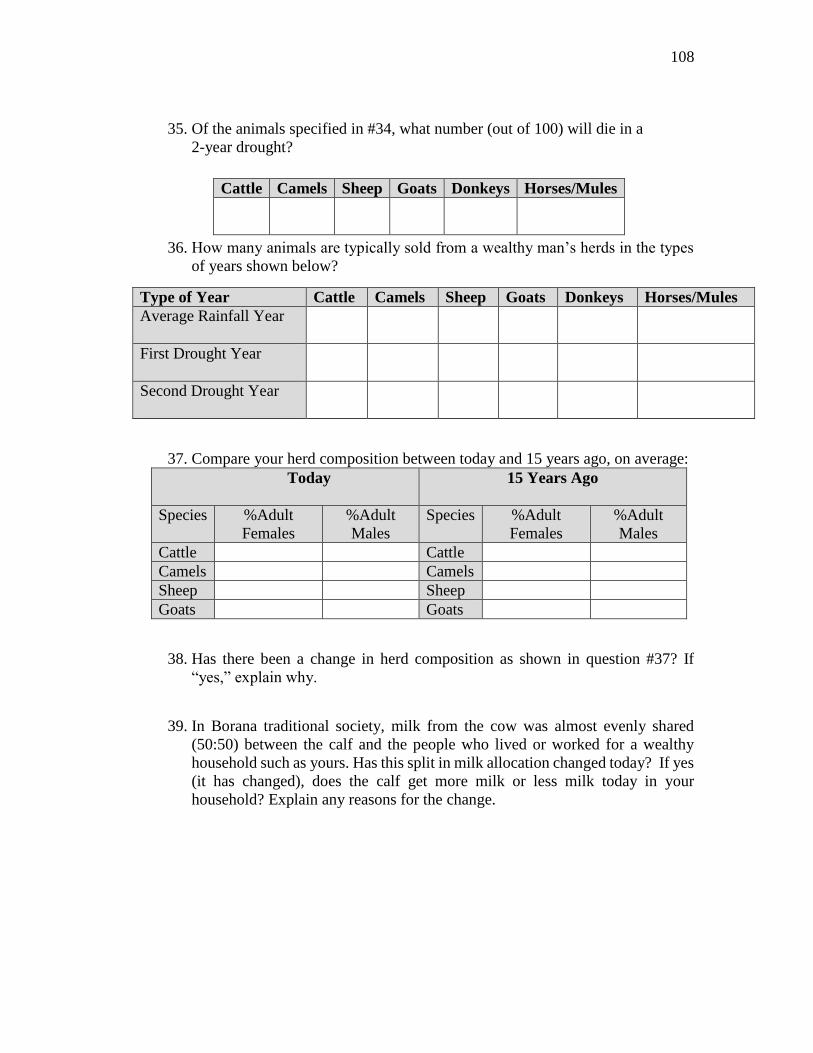
108
35. Of the animals specified in #34, what number (out of 100) will die in a
2-year drought?
36. How many animals are typically sold from a wealthy man’s herds in the types
of years shown below?
37. Compare your herd composition between today and 15 years ago, on average:
Today 15 Years Ago
Species %Adult
Females
%Adult
Males
Species %Adult
Females
%Adult
Males
Cattle Cattle
Camels Camels
Sheep Sheep
Goats Goats
38. Has there been a change in herd composition as shown in question #37? If
“yes,” explain why.
39. In Borana traditional society, milk from the cow was almost evenly shared
(50:50) between the calf and the people who lived or worked for a wealthy
household such as yours. Has this split in milk allocation changed today? If yes
(it has changed), does the calf get more milk or less milk today in your
household? Explain any reasons for the change.
Cattle Camels Sheep Goats Donkeys Horses/Mules
Type of Year Cattle Camels Sheep Goats Donkeys Horses/Mules
Average Rainfall Year
First Drought Year
Second Drought Year

109
40. Risk includes the chance for a herd to grow as well as the chance for a herd to
have losses. Rank the livestock species in terms of their overall level of risk for
you over a 10-year period. The number “1” indicates the most risky species
while the number “4” is the least risky species. If two livestock species have
the same risk, give them the same rank.
Category Rank
Cattle
Camels
Sheep
Goats
41. Using the same method as in #38, please rank the following investment options
in terms of their overall level of risk for you over the past 10 years. The number
“1” indicates the most risky while the number “6” is the least risky. For two
categories of the same risk, give them the same rank. If any categories cannot
be ranked, leave them out of the exercise.
Category Rank
All livestock species together
Banking
Property
Cultivation
Business
Your children

110
42. Specify the investment risk for categories below when compared with cattle
over the past 10 years.
Category
Categories
Banking Property Cropland Kalo Business Your Children
10x More
5x More
2x More
Equal
2x Less
5x Less
10x Less
43. If you are invested in non-pastoral options (like a home in town, hotel, business,
vehicles, etc.), where did you get the idea to do this? Please explain. If you are
not invested in non-pastoral options, please explain why not.
44. What investments are you most interested in making that you are not already
involved with? What most limits you from making these new investments?
Please explain.