ANALYSIS OF ONE DIMENSIONAL MOTION

Juan A. González, and Claudio Guerra-Vela. Department of Physics and Electronics. University of Puerto Rico at Humacao. Sponsored by the National Science Foundation (NSF) © All rights reserved (2006)

1

Experiment 3

ANALYSIS OF ONE DIMENSIONAL MOTION

Objectives 1. To establish a mathematical relationship between the position and the velocity of an object in motion. 2. To define the velocity as the change in the displacement of an object with respect to time. 3. To obtain a graph of the position versus time of a student in motion using the position sensor. 4. To make use of the software “Data Studio” to study different types of motion using a graph and to calculate the

velocity of the object in each case. 5. To explain that the description of any type of motion requires a reference frame.

Theory Definitions

Motion is the change in the position of an object with respect to other objects or with respect to a fixed point of reference. For now, and for simplicity, we shall only work with point objects in order to avoid effects related to rotational motion. A point object is defined as one that does not have any spatial dimensions; its size can be reduced to a geometrical point. The displacement vector, r, defines the direction and magnitude of the changes in the objects’ position. Mathematically,

r = ∆x = xf – xi 3-1

where xf is the final position and xi, the initial position. The distance, r, is the magnitude of the displacement, r =| r |. Both distance and displacement have the same units in the International System of units (SI), it is the meter, abbreviated m. The average speed, s, of an object is the total distance, d, traveled by the object, divided by the total time of travel, t. Mathematically,

tds = 3-2

We note that the speed is a scalar quantity while the average velocity, v, is a vector quantity. It is defined

as the displacement divided by the time interval during which the displacement takes place,

t= rv 3-3

The instantaneous velocity is defined as,

ddt

= rv 3-4

The instantaneous speed, s, is defined as the magnitude of the instantaneous velocity, s = | v |. Note that we

have used the same symbol to denote the average speed and the instantaneous speed even though they are conceptually different. The average acceleration, a, is the change in velocity divided by the time during which the change takes place. If vf is the final velocity and vi, the initial velocity then,

f= i-t

v va 3-5

The instantaneous acceleration is,


2

ddt

= va 3-6

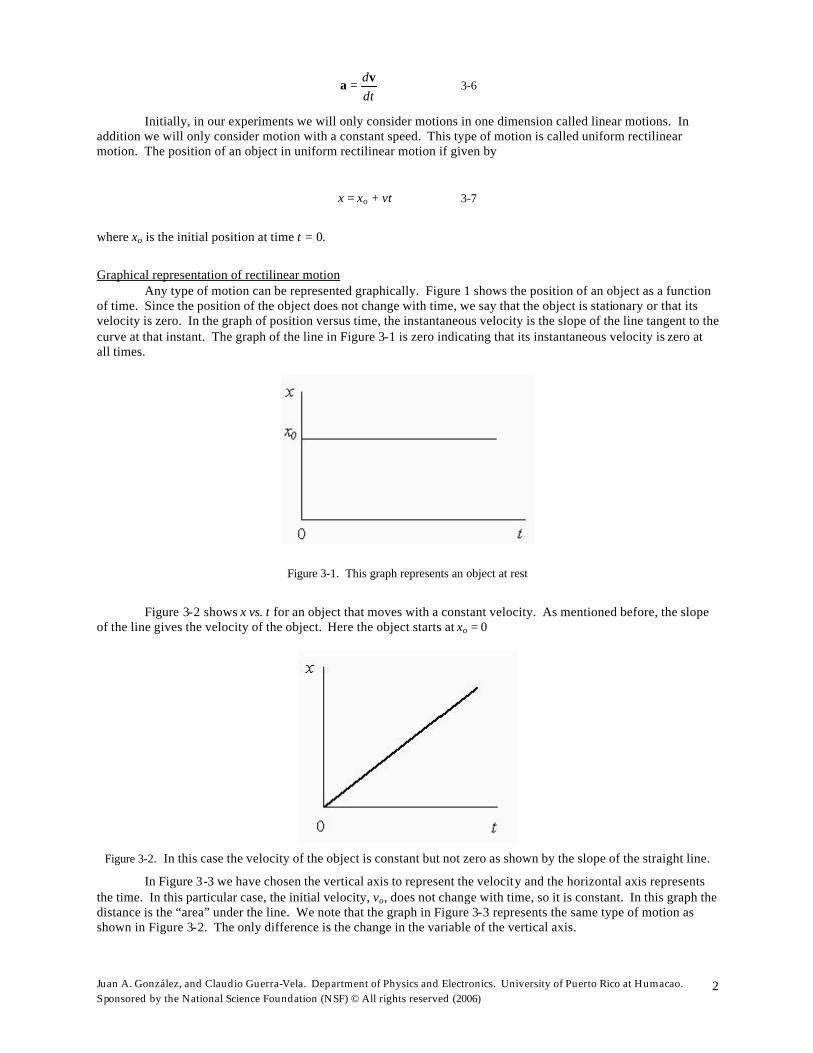
Initially, in our experiments we will only consider motions in one dimension called linear motions. In addition we will only consider motion with a constant speed. This type of motion is called uniform rectilinear motion. The position of an object in uniform rectilinear motion if given by

x = xo + vt 3-7

where xo is the initial position at time t = 0.

Graphical representation of rectilinear motion Any type of motion can be represented graphically. Figure 1 shows the position of an object as a function

of time. Since the position of the object does not change with time, we say that the object is stationary or that its velocity is zero. In the graph of position versus time, the instantaneous velocity is the slope of the line tangent to the curve at that instant. The graph of the line in Figure 3-1 is zero indicating that its instantaneous velocity is zero at all times.

Figure 3-1. This graph represents an object at rest

Figure 3-2 shows x vs. t for an object that moves with a constant velocity. As mentioned before, the slope

of the line gives the velocity of the object. Here the object starts at xo = 0

Figure 3-2. In this case the velocity of the object is constant but not zero as shown by the slope of the straight line.

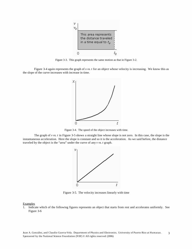
In Figure 3-3 we have chosen the vertical axis to represent the velocity and the horizontal axis represents the time. In this particular case, the initial velocity, vo, does not change with time, so it is constant. In this graph the distance is the “area” under the line. We note that the graph in Figure 3-3 represents the same type of motion as shown in Figure 3-2. The only difference is the change in the variable of the vertical axis.


3

Figure 3-3. This graph represents the same motion as that in Figure 3-2.

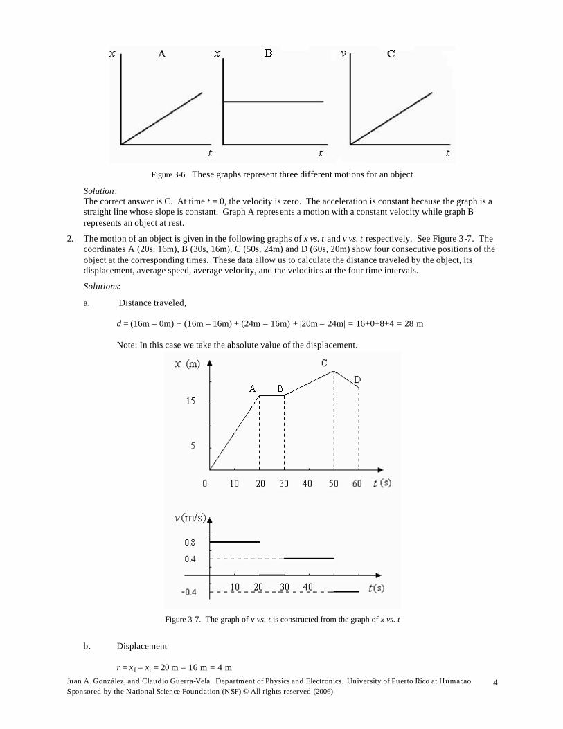
Figure 3-4 again represents the graph of x vs. t for an object whose velocity is increasing. We know this as

the slope of the curve increases with increase in time.

Figure 3-4. The speed of the object increases with time.

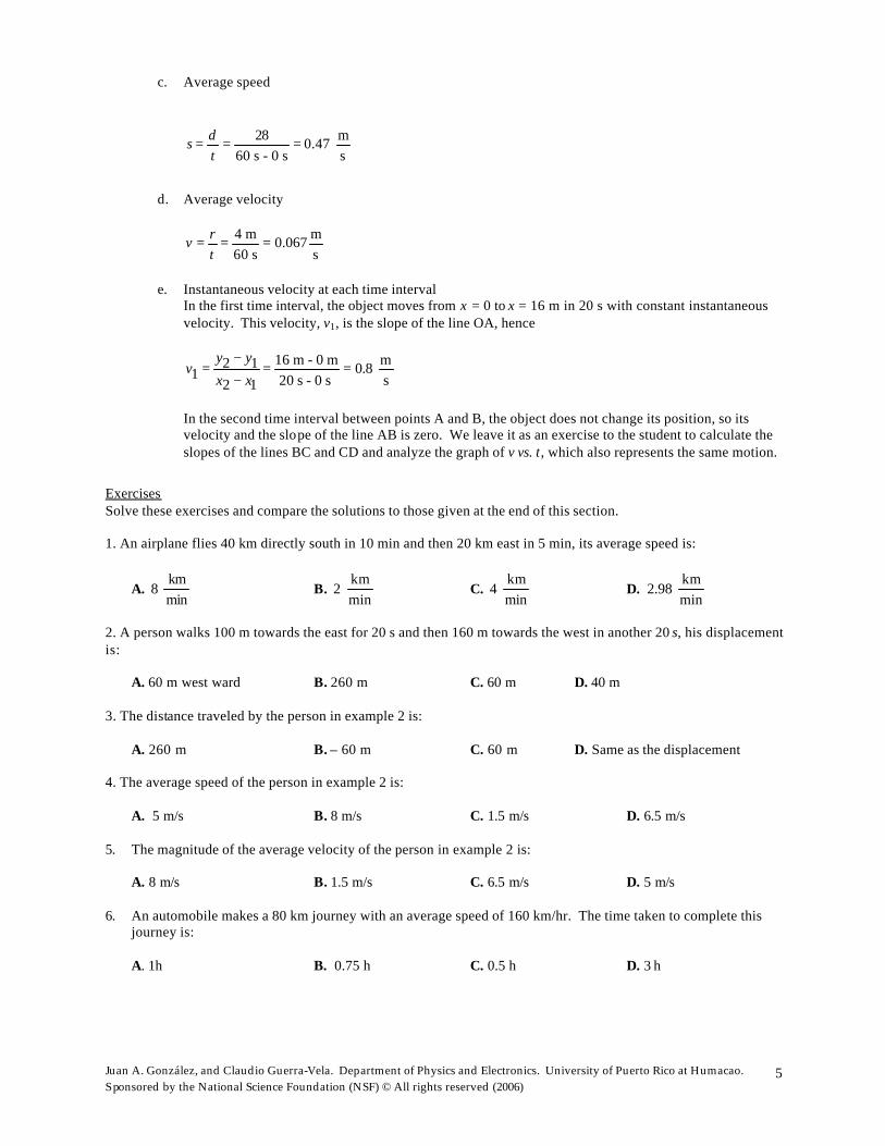
The graph of v vs. t in Figure 3-5 shows a straight line whose slope is not zero. In this case, the slope is the instantaneous acceleration. Here the slope is constant and so it is the acceleration. As we said before, the distance traveled by the object is the “area” under the curve of any v vs. t graph.

Figure 3-5. The velocity increases linearly with time

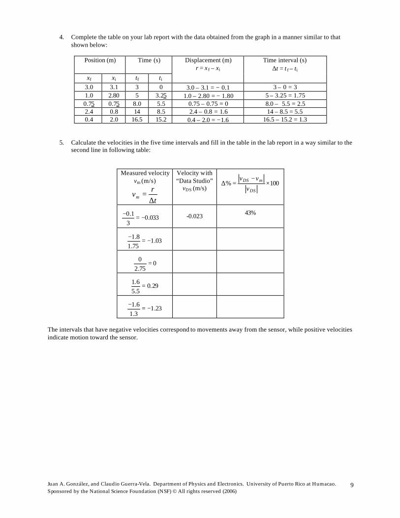
Examples 1. Indicate which of the following figures represents an object that starts from rest and accelerates uniformly. See

Figure 3-6


4

Figure 3-6. These graphs represent three different motions for an object

Solution: The correct answer is C. At time t = 0, the velocity is zero. The acceleration is constant because the graph is a straight line whose slope is constant. Graph A represents a motion with a constant velocity while graph B represents an object at rest.

2. The motion of an object is given in the following graphs of x vs. t and v vs. t respectively. See Figure 3-7. The coordinates A (20s, 16m), B (30s, 16m), C (50s, 24m) and D (60s, 20m) show four consecutive positions of the object at the corresponding times. These data allow us to calculate the distance traveled by the object, its displacement, average speed, average velocity, and the velocities at the four time intervals.

Solutions:

a. Distance traveled,

d = (16m – 0m) + (16m – 16m) + (24m – 16m) + |20m – 24m| = 16+0+8+4 = 28 m

Note: In this case we take the absolute value of the displacement.

Figure 3-7. The graph of v vs. t is constructed from the graph of x vs. t

b. Displacement

r = x f – xi = 20 m – 16 m = 4 m


5

c. Average speed

28 m0.47 60 s - 0 s s

dst

= = =

d. Average velocity

4 m m0.06760 s s

rvt

= = =

e. Instantaneous velocity at each time interval

In the first time interval, the object moves from x = 0 to x = 16 m in 20 s with constant instantaneous velocity. This velocity, v1, is the slope of the line OA, hence

16 m - 0 m m2 1 0.8 1 20 s - 0 s s2 1

y yv

x x

−= = =

−

In the second time interval between points A and B, the object does not change its position, so its velocity and the slope of the line AB is zero. We leave it as an exercise to the student to calculate the slopes of the lines BC and CD and analyze the graph of v vs. t, which also represents the same motion.

Exercises Solve these exercises and compare the solutions to those given at the end of this section. 1. An airplane flies 40 km directly south in 10 min and then 20 km east in 5 min, its average speed is:

A. km

8 min

B. km

2 min

C. km

4 min

D. km

2.98 min

2. A person walks 100 m towards the east for 20 s and then 160 m towards the west in another 20 s, his displacement is:

A. 60 m west ward B. 260 m C. 60 m D. 40 m 3. The distance traveled by the person in example 2 is:

A. 260 m B. – 60 m C. 60 m D. Same as the displacement

4. The average speed of the person in example 2 is:

A. 5 m/s B. 8 m/s C. 1.5 m/s D. 6.5 m/s 5. The magnitude of the average velocity of the person in example 2 is:

A. 8 m/s B. 1.5 m/s C. 6.5 m/s D. 5 m/s 6. An automobile makes a 80 km journey with an average speed of 160 km/hr. The time taken to complete this

journey is:

A. 1h B. 0.75 h C. 0.5 h D. 3 h


6

Solutions:

1. The average speed is defined as the total distance traveled divided by the total time taken,

40 km 20 km 60 km km1 2 4 10 min 5 min 15 min min1 2

x xs

t t

+ += = = =+ +

, so the answer is C

2. The two displacements and their resultant can be expressed via the vectors in the figure below:

R = A + B or R = A – B = 100 m – 160 m = -60 m, the correct answer is C. Remember from the laboratory dealing with vectors, that the resultant vector starts from the tail of the first vector and ends on the tip of the second vector after placing this second vector on the tip of the first vector.

3. The distance is the sum of the magnitudes of the displacements,

d = 100 m + -160 m = 260 m.

Note: The displacement of 160 m is negative as it is towards the left, nevertheless to calculate the distance traveled we treat it as positive as we are concerned only with the magnitude and not the direction.

4. As in example 1, the average speed is defined as the total distance traveled divided by the total time taken,

100 m 160 m 260 m m1 2 6.5

20 s 20 s 40 s s1 2

x xs

t t

+ += = = =+ +

, so the correct answer is D

5. The average velocity is the displacement divided by the time, so

60 m m1.540 s s

v −= = −

Since we need the magnitude of the velocity, we take the absolute value of the result v = - 1.5 m/s = 1.5 m/s. The correct answer is B.

6. The average speed is defined as s = d/t, hence we solve for t as, the correct answer is C.

80 km0.5 hkm

160 h

dt

s= = =

The motion sensor In this activity we will familiarize ourselves with uniform rectilinear motion by using the motion sensor

and plotting graphs of the position of a moving object with respect to time. This sensor together with “Data StudioTM” produces the graph of the position of a student as he moves along a straight line with varying velocities. The student must move in a manner such that the resulting graph can be interpreted according to the uniform rectilinear model. To describe the motion of an object with respect to a reference point, we need its velocity, and its acceleration. An instrument that does this is the motion sensor that emits pulses of ultrasound that get reflected from


7

the object to determine its position. While the object is in motion, the sensor measures many times in one second the change in its position. These changes in a given t ime interval are used to calculate the velocity of the moving object in meters per second. In the same way the change in velocity in a given time interval is used to calculate the acceleration in meters per second per second.

Materials and Instruments • Computer and the program “Data Studio” • Motion sensor • Pasco Interface 750 • Support stand with a metal bar • A heavy and thick flat surface to act as a reflecting screen for the ultrasound waves emitted by the motion

sensor. A book may work

Procedure 1. Open “Data Studio”, select “Create Experiment” and the motion sensor that is located in the list of sensors on

the left of the screen in the Pasco Interface 750 2. Mount the motion sensor to a support rod facing the person who moves back and for in front of the motion

sensor during the experiment. See Figure 3-8. Note the flat heavy screen carried by the student that reflects the ultrasound wave emitted by the sensor

3. Make sure that the moving student can walk at lease 2 m toward or away from the motion sensor 4. Connect the yellow cable of the sensor to channel 1 and the black cable to channel 2 on the interface 5. Place the computer monitor screen in such a way that the moving student can see the displayed results in real

time 6. In ‘Data Studio” select the graphical representation for the data and choose the position-time option 7. Adjust the scale from a minimum of 0 m to a maximum of 2 m and calibrate the sensor for a distance of one

meter. See “How to Configure and Calibrate the Motion Sensor” in the section “Starting Data Studio” in the laboratory manual

Figure 3-8. A student moves back and for in front of the motion sensor.

Data Get ready to locate your initial position. 1. Read this section before beginning taking data 2. Once the experiment has been programmed, the student must stand at least two meters away from the motion

sensor. At a given time another student must press the “Start” button on the computer 3. After 2 or 3 seconds, the student in front of the sensor must walk with a constant velocity of about 2 to 3 feet

per second and stop for about 2 seconds then walk back about halfway and finally walk with an increased velocity close toward the sensor. If the students followed the instruction above the graph should look something like the one in Figure 3-9.


8

Figure 3-9. Data acquired by the motion sensor

Calculating the velocity at different time intervals.

1. In the graph menu, select the Fit button and select Linear Fit. 2. Select the portion of the curve that is needed for the fitting using the mouse. 3. Repeat this procedure for each segment of the curve and make a note of the slope of the line fit, which

represents the velocity for each interval that you selected with the yellow section of the curve.

Figure 3-10. How to make a curve fit for the data selected in the graph


9

4. Complete the table on your lab report with the data obtained from the graph in a manner similar to that shown below:

Position (m) Time (s)

xf xi tf ti

Displacement (m) r = x f – xi

Time interval (s) ∆t = t f – ti

3.0 3.1 3 0 3.0 – 3.1 = − 0.1 3 – 0 = 3 1.0 2.80 5 3.25 1.0 – 2.80 = − 1.80 5 – 3.25 = 1.75 0.75 0.75 8.0 5.5 0.75 – 0.75 = 0 8.0 – 5.5 = 2.5 2.4 0.8 14 8.5 2.4 – 0.8 = 1.6 14 – 8.5 = 5.5 0.4 2.0 16.5 15.2 0.4 – 2.0 = −1.6 16.5 – 15.2 = 1.3

5. Calculate the velocities in the five time intervals and fill in the table in the lab report in a way similar to the second line in following table:

Measured velocity vm (m/s)

tr

vm ∆=

Velocity with “Data Studio”

vDS (m/s) 100% ×

−=∆

DS

mDS

v

vv

033.03

1.0 −=−

-0.023

43%

03.175.1

8.1 −=−

075.20 =

29.05.56.1 =

23.13.16.1 −=−

The intervals that have negative velocities correspond to movements away from the sensor, while positive velocities indicate motion toward the sensor.


10

LABORATORY REPORT OF EXPERIMENT 3

Analysis of one dimensional motion Section_______ Bench _______

Date: _________________________________________________________ Students:

1. ________________________________________________________ 2. ________________________________________________________

3. ________________________________________________________

4. ________________________________________________________

1. There are various time intervals in the graph obtained in this section. Its velocity characterizes each one. Fill in

the table with your data in a manner similar to that shown in the theory.

Interval Position (m) Displacement (m) Time (s) Time interval (s) xf xi r = x f – xi tf ti ∆t = t f – ti A

B

C

D

E

2. Identify the sections where the student approaches the sensor, stays stationary and where he moves away from the sensor.


11

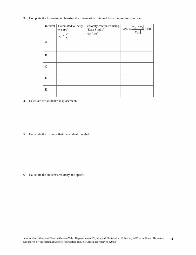
3. Complete the following table using the information obtained from the previous section

Interval Calculated velocity vc (m/s)

tr

v∆

=c

Velocity calculated using “Data Studio” vDS (m/s)

100% c ×−

=∆DS

DS

v

vv

A

B

C

D

E

4. Calculate the student’s displacement. 5. Calculate the distance that the student traveled. 6. Calculate the student’s velocity and speed.


12

Questions for Experiment 3

Analysis of one-dimensional motion This questionnaire has some typical questions of experiment 3. All students who are taking the course from laboratory of University Physics I must be able to correctly answer it before trying to make the experiment. 1. In the graph of position versus time, the slope of the curve is:

a. Velocity b. Acceleration c. Position d. No known quantity e. Force

2. An object moves in a straight line along the x-axis. Which one of the following positions corresponds to the biggest displacement? a. xi = 4 m, xf = 6 m b. xi = - 4 m, xf = - 8 m c. xi = - 4 m, xf = -2 m d. xi = - 4 m, xf = 2 m e. xi = - 4 m, xf = 4 m

3. An object moves in a straight line along the x-axis. Which one of the following positions corresponds to a negative displacement? a. xi = 4 m, xf = 6 m b. xi = - 4 m, xf = 4 m c. xi = - 4 m, xf = - 2 m d. xi = - 4 m, xf = 2 m e. xi = - 4 m, xf = - 8 m

4. The average speed of an object in a given time interval is defined as: a. Its velocity b. The total distance traveled divided by the total time of travel c. Half of the final velocity d. The acceleration multiplied by the time interval e. Half the acceleration multiplied by the time interval

5. Two automobiles are initially separated by a distance of 120 miles and approach each other. One travels at 35 mph and the other at 45 mph. They will meet in, a. 2.5 h b. 2.0 h c. 1.75 h d. 1.5 h e. 1.25 h

6. An automobile travels 30 miles with a speed of 60 mph and then travels another 30 miles at an speed 30 mph. Its average speed is, a. 35 mph b. 40 mph c. 45 mph d. 50 mph e. 53 mph

7. A graph of position versus time of an automobile is a straight line with a non-zero positive slope. The automobile has: a. A constant displacement that does not change with time b. An acceleration that increases as a function of time c. An acceleration that decreases as a function of time d. Constant velocity e. Increase in velocity


13

8. Which one of the following graphs represents an object moving with a constant velocity?

a. A b. B c. C d. D e. E

9. Which of the following graphs represents an object moving along a straight line with a constant velocity?



14

10. Which of the following graphs represents an object moving with an increase in its velocity?


The following questions, until the end of this exercise refer to the graph of position versus time of a person who walks for a tour as illustrated below:

11. The interval with zero velocity is, a. A b. B c. C d. D e. None of the above


15

12. The interval that represents negative velocity is,

a. A b. B c. C d. D e. None of the above

13. The interval that has the maximum velocity, a. A b. B c. C d. D e. None of the above

14. The velocity in the interval A is, a. 5.0 km/h b. Zero c. Negative d. 0.2 km/h e. 1.00 km/h

15. The displacement is, a. The area under curve b. 2.75 km c. 1.25 km d. The product of the average speed and the time of travel e. The distance covered during this time

16. The distance traveled is, a. 1.25 km b. The product of the average velocity and the time of travel c. 2.75 km d. Zero e. It cannot be determined from this graph

17. The average velocity is, a. The total distance traveled divided by the time of travel b. Zero c. 2.75 km/h d. Negative e. 1.25 km/h

18. The average speed is, a. Zero b. Insufficient data c. 1.25 km/h d. More than the average velocity e. 2.75 km/h

ANALYSIS OF ONE DIMENSIONAL MOTION

Documents

Transcript of ANALYSIS OF ONE DIMENSIONAL MOTION