Analysis of nutrient requirements for the Anaerobic ...

Analysis of nutrient requirements for the Anaerobic Digestion

of Fischer-Tropsch Reaction Water

By

Aarefah Mathir

In fulfilment of the MSc Chemical Engineering degree, College of

Agriculture, Engineering and Science, University of Kwa-Zulu Natal

Supervisors: Date of submission:

Dr KM Foxon 02 December 2013

Mr CJ Brouckaert

I

COLLEGE OF AGRICULTURE, ENGINEERING AND SCIENCE

DECLARATION - SUPERVISOR

I, ……………………………………….………………………., declare that as the candidate’s

Supervisor I agree to the submission of this thesis.

Signed

………………………………………………………………………………

II

COLLEGE OF AGRICULTURE, ENGINEERING AND SCIENCE

DECLARATION - PLAGIARISM

I, ……………………………………….………………………., declare that

1. The research reported in this thesis, except where otherwise indicated, is my original

research.

2. This thesis has not been submitted for any degree or examination at any other university.

3. This thesis does not contain other persons’ data, pictures, graphs or other information, unless

specifically acknowledged as being sourced from other persons.

4. This thesis does not contain other persons' writing, unless specifically acknowledged as being

sourced from other researchers. Where other written sources have been quoted, then:

a. Their words have been re-written but the general information attributed to them has been

referenced

b. Where their exact words have been used, then their writing has been placed in italics and

inside quotation marks, and referenced.

5. This thesis does not contain text, graphics or tables copied and pasted from the Internet,

unless specifically acknowledged, and the source being detailed in the thesis and in the

References sections.

Signed

………………………………………………………………………………

Form EX1-5

III

Acknowledgements

The author would like to acknowledge the following individuals:

K. M. Foxon for providing excellent guidance and supervision throughout the research

D. Teclu for running the UASB reactors needed to provide the seed sludge and for all the long

hours assisting with the analysis, even on short notice

My parents for keeping me inspired and humbled

My husband for your endless patience and much appreciated support

The author would also like to acknowledge:

Pollution Research Group for creating a great environment to work in

Sasol for providing the opportunity to perform this research

University of Kwa-Zulu Natal

IV

Executive Summary

Nutrients play an important role in the functioning of microorganisms during anaerobic digestion.

The anaerobic treatment of industrial wastewaters, such as Fischer-Tropsch Reaction Water

(FTRW), requires the addition of nutrients suitable for micro-organisms (micronutrients) since

these wastewaters are devoid of essential metals. However, the dosing of nutrients is only effective

if the metals are in a bioavailable form which in turn is dependent on the chemical speciation of the

system.

This study aimed to investigate and model the influence of precipitation on bioavailability by

considering the extent to which precipitation can sequester metals into forms that are not

bioavailable and the extent to which this sequestration can describe biological effects in an

anaerobic system. Visual MINTEQ and Excel were used to develop a combined mass balance and

chemical-equilibrium speciation model that considered the soluble and the precipitate metal phases.

The model was compared to two sets of experimental analysis. Experiment A included metal

analysis on the sludge and supernatant from glucose and ethanol fed ASBRs while Experiment B

included similar analysis on FTRW fed ASBRs while biological parameters were monitored during

a micro-metal washout experiment.

Precipitation was found to sequester Al, Zn and Fe to a large extent making them non-bioavailable

in Experiment A, while sulphide precipitates were predicted to dominate the metal speciation in

Experiment B. In Experiment A, the organically bound metals phase was also a significant phase

that sequestered metals. Furthermore, the rates of washout of most of the metals (excluding Mg)

were over-predicted, which may have been due to the absence of other solid related phases in the

model. This may also be attributed to kinetic effects in the system. Although there were reasonable

correlations between the model predicted and the experimentally determined concentrations, it is

recommended that the model should include the organically bound phase and consider mass

transfer effects in the system. After 12 cycles without dosing micro-metals in Experiment B, the

biogas production decreased by 43%. A decline in the predicted and determined soluble

concentrations of a variety of metals were observed during this time, suggesting that there may be

an agreement between predicted metals washout and reduction in anaerobic activity. Since the

soluble metal concentrations did not decrease as rapidly as predicted by the model, a lag period

between the two parameters was observed. Therefore, although the model provides an improved

understanding of metal speciation and bioavailability such that recommendations may be made for

prudent micro-metal dosing, further development is required for more accurate representations of

the system.

V

Table of Contents

Acknowledgements ........................................................................................................................... III

Executive Summary .......................................................................................................................... IV

Table of Contents ............................................................................................................................... V

List of Figures .................................................................................................................................... X

List of Tables ................................................................................................................................. XIII

1. Introduction ................................................................................................................................. 1

1.1 Background and motivation ................................................................................................ 1

1.2 Background into the Field ................................................................................................... 3

1.3 Aims and objectives ............................................................................................................ 5

2. Literature Review ........................................................................................................................ 6

2.1 Source and Properties of Reaction water ............................................................................ 6

2.2 Anaerobic Digestion............................................................................................................ 7

2.2.1 Favourable Conditions for Anaerobic Processing ....................................................... 7

2.2.2 Parameters used to determine efficiency of anaerobic digestion .............................. 13

2.3 Importance of nutrients in anaerobic digestion ................................................................. 14

2.3.1 Treatment of Industrial Streams ................................................................................ 17

2.3.2 Growth and functioning of Microorganisms ............................................................. 19

2.3.3 Settleability of the sludge .......................................................................................... 24

2.4 Bioavailability of Metals ................................................................................................... 24

2.5 Precipitation Chemistry ..................................................................................................... 26

2.6 Methods to determine Bioavailability in a system ............................................................ 28

2.6.1 Analytical Approach ................................................................................................. 28

2.6.2 Chemical Speciation Modelling ................................................................................ 33

2.7 Uptake of metals by the microorganisms .......................................................................... 35

2.8 Micronutrient dosing ......................................................................................................... 36

2.8.1 Dosing Strategy ......................................................................................................... 36

VI

2.8.2 Recipes Used ............................................................................................................. 37

2.9 Anaerobic Sequencing batch reactors ............................................................................... 39

2.9.1 Sequencing Batch Reactor operation ........................................................................ 39

2.9.2 Advantages and Disadvantages ................................................................................. 40

3. Research Methodology.............................................................................................................. 42

3.1 Experiment A .................................................................................................................... 44

3.1.1 Experimental setup .................................................................................................... 44

3.1.2 Reactor Operation ..................................................................................................... 46

3.1.3 Influent Composition ................................................................................................ 46

3.1.4 Sampling and Analytical Techniques ........................................................................ 48

3.2 Experiment B .................................................................................................................... 52

3.2.1 Experimental Setup ................................................................................................... 53

3.2.2 Seed sludge source .................................................................................................... 56

3.2.3 Initial operation ......................................................................................................... 57

3.2.4 Stable Operation ........................................................................................................ 57

3.2.5 Washout Experiment ................................................................................................. 58

3.2.6 Reactor Operation ..................................................................................................... 58

3.2.7 Sampling and Analytical Techniques ........................................................................ 60

3.3 Mass Balance-Chemical Speciation Modelling ................................................................ 62

3.3.1 Rationale ................................................................................................................... 62

3.3.2 Model Development .................................................................................................. 62

3.3.3 Assumptions .............................................................................................................. 63

4. Results ....................................................................................................................................... 69

4.1 Experiment A Results ....................................................................................................... 69

4.1.1 Metals Mass Balance ................................................................................................. 69

4.1.2 Sequential Extraction of Sludge ................................................................................ 71

4.1.3 Comparison between Acid Digestion and Sequential Extraction ............................. 73

VII

4.1.4 Mass Balance-Speciation Modelling Results- Experiment A ................................... 74

4.2 Experiment B Results ........................................................................................................ 80

4.2.1 Mass Balance-Speciation Modelling Results- Experiment B ................................... 82

4.2.2 Supernatant Metal Analysis ...................................................................................... 88

4.2.3 Sludge Metal Analysis .............................................................................................. 90

4.2.4 Bioprocess Results Calculation and Summary .......................................................... 93

4.2.5 Biogas production, methane activity and methane recovery ..................................... 96

4.2.6 pH Control ................................................................................................................. 97

4.2.7 Biogas production comparison to alkalinity dosage.................................................. 98

5. Discussion ............................................................................................................................... 100

5.1 Experiment A Discussion ................................................................................................ 100

5.1.1 Metals Mass Balance ............................................................................................... 100

5.1.2 Sequential Extraction of Sludge .............................................................................. 101

5.1.3 Comparison between Acid Digestion and Sequential Extraction ........................... 105

5.1.4 Mass Balance-Speciation Modelling Discussion- Experiment A ........................... 106

5.2 Experiment B Discussion ................................................................................................ 111

5.2.1 Mass Balance-Speciation Modelling Discussion- Experiment B ............................ 111

5.2.2 Supernatant Metal Analysis .................................................................................... 114

5.2.3 Sludge Metal Analysis ............................................................................................ 115

5.2.4 Biogas production, methane activity and methane recovery ................................... 118

5.2.5 pH Control ............................................................................................................... 119

5.2.6 Biogas production comparison to alkalinity dosage................................................ 120

5.2.7 Biogas production comparison to soluble metal concentration ............................... 121

5.2.8 Validity of Model Assumptions .............................................................................. 123

5.2.9 Dosing Strategy ....................................................................................................... 125

6. Conclusions and Recommendations ....................................................................................... 127

7. References ............................................................................................................................... 131

VIII

8. Appendix A-List of Micro-nutrient recipes from Literature ................................................... 140

9. Appendix B: Analytical Methods ............................................................................................ 150

9.1 ICP-AES Analysis ........................................................................................................... 150

9.1.1 Sample Preparation ................................................................................................. 150

9.1.2 Standard Solutions preparation ............................................................................... 150

9.1.3 Quality Control........................................................................................................ 151

9.2 Acid Digestion of Sludge ................................................................................................ 152

9.2.1 Apparatus and Reagents .......................................................................................... 152

9.2.2 Method .................................................................................................................... 152

9.2.3 Obtaining the sludge samples for acid digestion ..................................................... 153

9.2.4 Calculating the total amount of metals in the reactor .............................................. 154

9.3 Sequential Extraction ...................................................................................................... 155

9.3.1 Apparatus and Reagents .......................................................................................... 155

9.3.2 Method .................................................................................................................... 156

10. Appendix C: Initial Conditions for Mass Balance-Speciation Modelling .......................... 158

11. Appendix D: Illustration of the Mass balance in the Mass balance-Speciation model ....... 160

11.1 Mass balance for Experiment A ...................................................................................... 160

11.2 Mass balance for Experiment B ...................................................................................... 160

12. Appendix E: Mass balance-Speciation Modelling for Experiment A, Reactor II. .............. 162

12.1.1 Soluble Concentration Changes .............................................................................. 162

12.1.2 Precipitate Formation .............................................................................................. 165

13. Appendix F: Experiment B results for Reactor I ................................................................. 168

13.1 Results Summary ............................................................................................................ 168

13.2 Biogas Production, methane activity and methane recovery .......................................... 168

13.3 pH Control ....................................................................................................................... 169

13.4 Biogas production comparison to alkalinity dosage ....................................................... 170

13.5 Supernatant Metal Analysis ............................................................................................ 172

IX

13.6 Sludge Metal Analysis .................................................................................................... 173

X

List of Figures

Figure 1: Source of FTRW in the Sasol Oil-from-coal process .......................................................... 6

Figure 2: The series metabolism for the anaerobic digestion of synthetic compounds..................... 17

Figure 3: Fate of micro-metals when added to a reactor ................................................................... 25

Figure 4: Schematic representation of one cycle for a sequencing batch reactor. ............................ 39

Figure 5: Experimental setup of one reactor for Experiment A. ....................................................... 45

Figure 6: Metals mass balance for a reactor for one cycle. ............................................................... 51

Figure 7: Experiment B reactor setup ............................................................................................... 54

Figure 8: Lid configuration for reactors I and II in Experiment B. ................................................... 56

Figure 9: Metals mass balance (range 100-2000 mg) for Cycle (i) Reactor I and II. ....................... 70

Figure 10: Metals mass balance (range 0- 100 mg) for Cycle (i) Reactor I and II. .......................... 71

Figure 11: Sequentially extracted metal phases of Cycle (i) initial sludge (1), Cycle (i) final

sludge/Cycle (ii) initial sludge (2) and Cycle (ii) final sludge (3) for Reactor I and II. (Range 100-

2000 mg). Arrows indicate potentially bioavailable and non-bioavailable fractions. ....................... 72

Figure 12: Sequentially extracted metal phases of Cycle A initial sludge (1), Cycle A final

sludge/Cycle B initial sludge (2) and Cycle B final sludge (3) for reactor I and II. (Range 0-100

mg). ................................................................................................................................................... 73

Figure 13: Comparison of metals determined using acid digestion and sequential extraction for Al,

Zn, Fe and Mg for reactor I and II with standard deviations. ........................................................... 74

Figure 14: Concentration of ions in the dissolved phase for Ca, Fe, K and Mg ions, and their

changes with each successive cycle modelled for Reactor I, including comparisons to experimental

values for Fe and Mg (mg/l).............................................................................................................. 76

Figure 15: Concentration of ions in the dissolved phase for Mn, Cu and Zn ions (µg/l), and their

changes with each successive cycle modelled for Reactor I, including comparisons to experimental

values for Cu and Zn. ........................................................................................................................ 77

Figure 16: Concentration of ions in the dissolved phase for Co2+

and HS-1

(μg/l), and their changes

with each successive cycle modelled for Reactor I. .......................................................................... 78

Figure 17: Percentage of ions that are within precipitates as predicted for each successive cycle

modelled together with the values obtained from experimental data for Mg, Ca, Fe, Cu and Zn. ... 79

Figure 18: Model prediction of the concentrations of different precipitates formed and their changes

with each cycle modelled. ................................................................................................................. 82

Figure 19: Percentages of the metal ions found within precipitates and their changes with each

cycle modelled. ................................................................................................................................. 83

XI

Figure 20: Concentration of ions in the dissolved phase for Mg and Ca, and their changes with each

successive cycle modelled for Reactor II, including comparisons to experimental values. .............. 84

Figure 21: Concentration of ions in the dissolved phase for Mn (in mg/l x10-4) and Zn (in mg/l

x10-8) and their changes with each successive cycle modelled for Reactor II. ................................ 85

Figure 22: Concentration of ions in the dissolved phase for Co, Fe and Ni as predicted by the

model. ................................................................................................................................................ 86

Figure 23: Concentration of Fe ions in the dissolved phase as predicted by the model compared to

the experimentally determined values ............................................................................................... 87

Figure 24: Washout pattern observed for the soluble concentrations of Cu and Mo (as MoO42-

) as

predicted by the model ...................................................................................................................... 88

Figure 25: Measured soluble concentrations as a percentage of the maximum concentration

measured as well as the amount of metal lost as a % of the feed for selected cycles only. .............. 89

Figure 26: Sludge metal concentrations as a function of the maximum concentration measured for

selected cycles for Al, Ca, Co, Cr, Cu, Fe, Mg, Mn and Zn. ............................................................ 90

Figure 27: Comparison between reactor I and reactor II experimental values for the measured

sludge concentrations as a percentage of the maximum sludge concentration from both reactors

(Cref), for selected cycles only. ........................................................................................................ 91

Figure 28: Amount of metal retained within Reactor II as a percentage of the amount dosed via the

feed for selected cycle for Ca, Co, Cu, Fe, Mg , Mn and Zn. ........................................................... 92

Figure 29: The MATLAB graph output for Cycle -3 showing from left to right, cumulative gas

production, gas composition evolution and cumulative methane production with time. .................. 94

Figure 30: The Total biogas production and % methane recovery on the left axis and maximum

methane activity for pre-metal washout cycles -3 to -1 and post-metal washout cycles 0 to 15 on the

right axis. ........................................................................................................................................... 96

Figure 31: Time required to reach pH recovery and the subsequent increment in dosage for the

following cycle for Reactor II. .......................................................................................................... 97

Figure 32: Comparison between Total biogas produced and alkalinity dosed for cycles -3 to 15,

Reactor II........................................................................................................................................... 98

Figure 33: Comparison of biogas production data with the experimental soluble metal concentration

for Mg, Ca and Fe and the model predicted cycle at which metal soluble concentration starts to

decrease (in green boxes) ................................................................................................................ 121

Figure 34: : Concentration of ions in the dissolved phase for Ca, Fe, K and Mg ions, and their

changes with each successive cycle modelled for Reactor II, including comparisons to experimental

values for Fe and Mg (mg/l)............................................................................................................ 162

XII

Figure 35: Concentration of ions in the dissolved phase for Mn, Cu and Zn ions (µg/l), and their

changes with each successive cycle modelled for Reactor II, including comparisons to experimental

values for Cu and Zn. ...................................................................................................................... 164

Figure 36: Concentration of ions in the dissolved phase for Co2+

and HS-1

(μg/l), and their changes

with each successive cycle modelled for Reactor II. ...................................................................... 165

Figure 37: Percentage of ions that are within precipitates as predicted for each successive cycle

modelled. ......................................................................................................................................... 166

Figure 38: The Total biogas production and % methane recovery on the left axis and maximum

methane activity for pre-metal washout cycles -3 to -1 and post-metal washout cycles 0 to 15 on the

right axis for Reactor I. ................................................................................................................... 169

Figure 39: Time required to reach pH recovery and the subsequent increment in dosage for the

following cycle for Reactor I. ......................................................................................................... 170

Figure 40: Comparison between Total biogas produced and alkalinity dosed for cycles -3 to 15,

Reactor I. ......................................................................................................................................... 171

Figure 41: Soluble concentrations as a percentage of the maximum concentration as well as the

amount of metal washout as a % of the feed for cycles -2, 9 and 15, Reactor I. ............................ 172

Figure 42: Sludge metal concentrations as a percentage of the maximum concentration for selected

cycles for Al, Ca, Co, Cr, Cu, Fe, Mg, Mn and Zn, Reactor I. ....................................................... 173

Figure 43: Amount of metal retained within Reactor I as a percentage of the amount dosed via the

feed for selected cycles. .................................................................................................................. 174

XIII

List of Tables

Table 1: Reported toxic concentrations of metals and their effects on various systems. .................. 11

Table 2: Reported stimulatory/optimum concentrations of metals added for various systems ......... 15

Table 3: Role of micronutrients in microbial systems ...................................................................... 21

Table 4: Roles of trace metals in enzymes involved in anaerobic reactions and transformations

(Fermoso et al., 2009). ...................................................................................................................... 22

Table 5: Role of Some Vitamins in microbiological processes ........................................................ 24

Table 6: Solubility products for certain compounds in water at 25°C .............................................. 28

Table 7: Outline of Stover and Modified Tessier extraction schemes .............................................. 31

Table 8: Nutrient recipe used by Sasol for their anaerobic digestion of FTRW ............................... 38

Table 9: Operating parameters for each sequencing batch reactor ................................................... 46

Table 10: Influent Composition for Reactors I and II, Experiment A. ............................................. 47

Table 11: Nutrient medium solution as proposed by Owen et al, 1979. ........................................... 47

Table 12: Stover Scheme overview ................................................................................................... 52

Table 13: Influent Composition for ASBRs, Experiment B. ............................................................ 58

Table 14: Operating parameters for the ASBRs, Experiment B. ...................................................... 59

Table 15: GC Specifications ............................................................................................................. 61

Table 16: Precipitates likely to form under Experimental Conditions. ............................................. 65

Table 17: Metals Inventory. .............................................................................................................. 69

Table 18: Summary of experimental results for cycles -3 to 15 for Reactor II. ................................ 95

Table 19: Nutrient Recipes used in Literature and their values compared to the recipe used by Sasol

......................................................................................................................................................... 141

Table 20: Reagent Scheme for the sequential extraction procedure ............................................... 157

Table 21: Initial Concentrations used in VM for Experiment A, Reactors I and II ........................ 158

Table 22: Initial Concentrations used for Experiment B ................................................................. 159

Table 23: Summary of experimental results for cycles -3 to 15 for Reactor I. ............................... 168

1

1. Introduction

1.1 Background and motivation During the Sasol Fischer-Tropsch synthesis process, synthesis gas (CO2 and H2) reacts over an iron-

based catalyst to produce methane, water and CnH2n hydrocarbons in the C1 to C20 range. A high

COD effluent stream composed mainly of short chain fatty acids (SCFAs), referred to as Fischer-

Tropsch Reaction water (FTRW), is a by-product of this process. Treatment of this stream is

required before re-entering the water circuit and is currently performed using aerobic treatment.

Anaerobic digestion is being investigated as an alternative, since it eliminates the energy intensive

aeration requirements and produces between 5 and 10 times less sludge (Steyer et al., 2006).

Coupled with this is the advantage of a high biogas or methane production due to the high

concentration of fatty acids in the effluent (Martinez-Sosa et al., 2009).

Microscopic organisms are responsible for the actual degradation by utilizing the organic matter as

nourishment. For these microorganisms to function well, a variety of nutrients are required for

growth, metabolic and enzymatic functions (Fermoso et al., 2009). In municipal anaerobic

digestion, the wastewater being treated contains a mixture of micronutrients from different

applications of domestic water, commercial use and storm water (Kroiss & Zessner, 2001). In

contrast, industrial wastewater is a product of one or a few processes with the composition defined

by the waste products of those processes. The nutrients present for microbial growth will therefore

be limited to the chemical and biological components which are generated by those processes and

certain essential micronutrients may be completely absent from the waste stream.

Nutrients in anaerobic digestion may be divided into three categories, namely macronutrients,

micronutrients and vitamins. Macronutrients refer to those elements that are required in large

concentrations (above 1 mg/l). Micronutrients are those trace metals that are required in

concentrations in the range of less than 1 mg/l. FTRW, a petro-chemical industry effluent, contains

appreciable amounts of nutrients such as Fe (from the Fe-based catalyst) due to the process itself.

However it is deficient in most of the nutrients such as N, P, K and S and other micronutrients such

as Cu, Zn, Al, Co and Ni that are necessary for the functioning of the microorganisms. It is also

unknown whether micronutrients that are present are in a form the microbes are able to assimilate.

Anaerobic treatment of this effluent therefore requires nutrient supplementation.

2

In the wastewater treatment of an industrial effluent, the biodegradation of complex and synthetic

compounds are sometimes necessary. To overcome this hurdle, a variety of biodegradation

pathways are required through a consortium of anaerobic microorganisms (Burgess et al., 1999).

Sustenance of such a diverse microbial population necessitates a composite and sufficient

micronutrient supplementation.

In the available literature, many authors have suggested nutrient supplement recipes (Owen et al.,

1979, Speece, 1996, Fermoso, 2008, etc.). A comprehensive list of these recipes together with their

references may be found in Appendix A. However, effluents produced by different types of

industries will differ in their composition and concentration of the micro-metals present. The types

of microorganisms within the digesters will also be different. Thus each effluent will require a

micronutrient mix suitable for that effluent and process. Sasol currently dose nutrients according to

a recipe obtained from internal studies on growth kinetics (Du Preez et al., 1987 as cited in Van

Zyl, 2008). It is not known whether this recipe is ideal in terms of the amounts used and actual

nutrients required for this type of effluent stream.

Macronutrient requirements are generally well known and documented, usually expressed as a ratio

to the carbon in the waste water. Micronutrient requirements, however, have not been fully

understood as the interactions of micronutrients (when dosed to a solution) with their surroundings

are complex. These include interactions within the aqueous phase, with the microorganisms and

other solid phases in the digester and even with the materials of construction of the digester itself.

These factors are important as they affect the phases in which metals will exist and the quantities

thereof. This in turn affects the bioavailability, defined as the condition of the metal such that it can

or cannot be biologically assimilated into a microorganism for use in metabolic processes.

Conversely, metals which are present in a form that is not bioavailable may be present in large

concentrations but with no beneficial effect to the biological process. Dosing response experiments

consider the effect on biological activity of a change in the dose of micronutrients and will

therefore provide information only applicable to that particular system under investigation; should

the conditions of that system be investigated, or a new system is being investigated, then a new set

of dosing response experiments will be required.

Metals may exist in the following phases when added to a system:

As a free or inorganic complexed soluble ion.

On the exterior of the cell or sludge flocs through adsorption.

As a solid inorganic precipitate.

3

As an organically complexed ion.

Within the actual cells after absorption has occurred.

Free and inorganically complexed soluble metal ions may be considered as bioavailable (Speece,

1996) while adsorbed metal ions, metal ions locked within precipitates and organically complexed

ions may be considered potentially bioavailable. The understanding behind this is that in their

current phase, the metal ions are not bioavailable however when system conditions change, such as

a drop in pH, metal ions may be released from any of those phases into a bioavailable form. Current

knowledge suggests that the free soluble metal ion concentration may be key to the bioavailability

of the metal; therefore understanding the speciation chemistry for ionic constituents within a system

and in particular the factors that dictate the amount of soluble metal ions may therefore be

important for understanding bioavailability, and specifically for predicting the influence of a

particular metal dosing strategy on biological activity.

The current state of the art for research into micronutrient requirements involves investigating the

speciation of metal ions within a sample of anaerobic digester mixed liquor analytically using a

sequential extraction technique; this method uses a sequence of different reagents to extract metals

from different phases within the sample (Aquino and Stuckey, 2007, van Hullebusch et al., 2005,

Fermoso, 2008). Sequential extraction procedures are often hampered by difficulties in determining

trace metal concentrations, due to the small concentrations the trace metals which are also found in

the sequential extraction process, resulting in further dilution of the metals which are sometimes

below detection limits. Concerns about disrupting speciation due to sampling and extraction steps

have been expressed (Nordstrom, 1996; Filgueras et al., 2002).

There is no systematic way of predicting bioavailability from first principles reported in the

literature. This project therefore represents a first attempt to develop a theory for modeling

bioavailability of micronutrients in anaerobic digesters.

1.2 Background into the Field There is a range of micronutrient concentrations where the metabolic rate of anaerobic digestion is

not reduced due to limitation of availability of any of the metals, and it is not inhibited by a high

concentration of any of the metals. Numerous investigations have been reported in the literature,

where these ranges of concentrations have been found for a number of scenarios with different

reactors, substrates and operating conditions (Speece, 1996). In all of these cases, ranges or

stimulatory concentrations have been determined analytically using dosage response experiments.

However, these dosage response experiments provide ranges of micronutrient concentrations that

4

apply for the experimental setup used for the investigation and there are often significant

discrepancies between the dosing ranges proposed by different researchers. Should experimental

conditions change, a new set of dosage response experiments is required.

Historically, speciation and thus bioavailability have been determined analytically (Aquino and

Stuckey, 2007, van Hullebusch et al., 2005, Fermoso, 2008). Free metal ion concentrations have

been found using a number of techniques including ion selective electrodes, atomic absorption

spectroscopy and ion exchange equilibrium techniques. Speciation including other categories such

as adsorbed and precipitated ions has been undertaken analytically using sequential solvent

extraction techniques. These are however operationally defined categories as they are dependent

upon the solvent used for the extraction.

Static metal speciation modelling to determine the heavy metal toxicity of soils, sediments and

aquatic systems has been performed (Nordstrom, 1996, Tipping et al., 1998, Huber et al., 2002).

Although useful in assessing the speciation of a sample at a particular point, it provides no

indication of how the speciation changes with time. Chemical speciation modeling also has certain

limitations such as many speciation models are equilibrium based and this may not always be

applicable for the system being modeled.

Dynamic modelling of biological processes in anaerobic liquor has been developed over the past

few years. The first stage included modelling of simple biochemistry involved in the digestion

process. The second stage covered complex biochemistry where different anaerobic

microorganisms were assigned different growth and death rates. Ionic speciation was incorporated

in the third stage of development (Van Zyl et al., 2008). Although this dynamic modelling of

anaerobic liquor is comprehensive, it does not include metals and their speciation at this stage (Van

Zyl et al., 2012).

Literature indicates that precipitation, adsorption and complexation can all sequester metal ions,

making them biologically unavailable or potentially bioavailable (but not currently bioavailable)

when the sequestration process is reversible. Metal speciation, its interactions with other organic

and inorganic ions and its distribution between the different phases (soluble, adsorbed, organically

complexed and precipitated) is complex and thus cannot be simply integrated into an existing

dynamic bioprocess model. There are only a few cases of dynamic metal speciation modelling that

incorporate metal precipitation (Musvoto et al., 2000). These models are based on reaction kinetics

of a weak acid/base system and metal precipitation reactions included are limited to Mg and Ca

with carbonate, ammonium and phosphate ions. Therefor to be able to predict biological response

5

to micronutrient dosing, it is necessary to develop a model that considers biological processes and

metal speciation chemistry.

1.3 Aims and objectives In literature, there is no speciation modelling approach to metal bioavailability in anaerobic

systems. This research is part of a Sasol-University Collaboration Programme grant in which the

micronutrient requirements for an anaerobic membrane bioreactor treating FTRW are being

investigated. The aim of the wider research is to investigate the relationship between metal

speciation and biological activity in an attempt to develop a model of metal bioavailability. The

ultimate objective of the research thrust is to undertake a critical analysis of the proposed

micronutrient dosing strategy and identify potential cost and environmental savings that could be

achieved by altering the dosing strategy. In order to do this, a fundamental understanding of the

dynamics of metals as micronutrients in the anaerobic digestion is required. This research is a new

excursion into the field but since there is a high degree of complexity to it, a stage-wise approach is

necessary. In the first step, the objective is to investigate and model the influence of precipitation

on bioavailability. This will be performed as follows:

Consider the extent to which precipitation can sequester metals into forms that are not

bioavailable; and

Consider the extent to which this sequestration can describe biological effects such as

methanogenic activity.

In this first step, the effect of metal sequestering processes other than precipitation (such as

adsorption and ion exchange) have been ignored in the development of a bioavailability model.

Although this is a significant simplification of the problem, the objective of the research is to

demonstrate order of magnitude effects, and therefore the simplest possible description of the

problem has been adopted.

Therefore a further objective is to

Assess whether the assumption that of all the possible metal sequestration effects, only

precipitation has a significant effect on bioavailability is valid and if not, which additional

effects should be considered in the next layer of model development.

6

2. Literature Review

2.1 Source and Properties of Reaction water Fischer-Tropsch (FT) reaction is a technology that has been employed by Sasol for over half a

century for the production of fuel from coal. Coal, in the presence of O2 and steam, is gasified at a

temperature of 1200 °C and a pressure of 3 MPa in Lurgi dry-ash gasifiers to produce synthesis gas

(CO and H2) (Dry, 2002). At Sasol Secunda, the synthesis gas is purified and subsequently sent to

Sasol Advanced Synthol reactors where H2 and CO react in the presence of an iron-based catalyst

to produce methane, water and hydrocarbons in the C1 to C20 range, according to the following

reaction (Van Zyl, 2008):

(1)

This is the high temperature FT synthesis which occurs between 300 and 350 °C (Dry, 2002).The

product stream is progressively cooled in a product recovery plant where the methane, water and

hydrocarbons produced are separated. The methane-rich stream is recycled back to the gasifiers

while the hydrocarbon products are used for gasoline and linear low molecular mass olefins (Dry,

2002). The water produced from the reaction contains a considerable amount of short chain fatty

acids (SCFA) which cannot be separated from the water economically (Van Zyl, 2008). This

mixture is called Fischer-Tropsch Reaction Water (FTRW), one of three waste streams produced

from this process. The figure that follows shows this process graphically.

Synthol Reactor

300-350°C

Lurgi Gasifier

1200°C, 3MPa

Coal

Oxygen

Steam

Syn Gas

Cooling

(Product Recovery)

Methane Rich Stream

FTRW

Hydrocarbon Product Stream

Figure 1: Source of FTRW in the Sasol Oil-from-coal process

7

Van Zyl (2008) describes this stream as containing mainly C2 to C6 SCFA with a pH of 3.77 and 35

mg/L of total dissolved solids. Sasol Secunda produces 29 ML/day of FTRW with an average COD

of 18 000 mg/L. This wastewater stream was initially treated at the Secunda activated sludge plant

with two other wastewater streams, namely stripped gas liquor, a waste stream as a result of

purifying synthesis gas, and oily sewer water which originates from plant drainage (Van Zyl, 2008).

FTRW currently makes up 23% of the stream to the activated sludge plant but contributes 77% of

the total organic load, thus contributing significantly to high oxygen, electricity and treatment costs

relating to the plant. Other problems associated with treating a stream rich in SCFA is a high solids-

liquid separation cost and production of an effluent high in suspended solids after secondary

settling. These are a result of the tendency to produce biomass that flocculates and settles poorly.

(Van Zyl, 2008).

As a solution to these problems, anaerobic digestion of FTRW has been proposed as an alternative

to an aerobic activated sludge system. Anaerobic digestion requires no oxygen, drastically reducing

the oxygen demands for the plant. It also produces between 5 to 10 times less sludge than aerobic

processes (Steyer et al., 2006), decreasing sludge handling costs. FTRW is a stream rich in organic

compounds (the SCFA); therefore the potential to recover energy in the form of methane rich

biogas is considerable.

2.2 Anaerobic Digestion Anaerobic digestion as a technology to degrade organic waste material has existed for over a

century. Although the advantages are well established, many industries are hesitant to apply this

technology (Chen et al., 2008). This is due to the sensitive relationship between variations in the

process operating conditions and the stability of the process. When the stability of the process has

been compromised, the digester requires several weeks to several months to recover, during which

no treatment may occur (Steyer et al., 2002). It is therefore necessary to keep conditions in the

digester as ideal as possible.

2.2.1 Favourable Conditions for Anaerobic Processing

There are several parameters which need to be considered in order to achieve efficient anaerobic

treatment. These include a favorable temperature and pH range, manageable toxicity levels,

adequate nutrients, a carbon source, sufficient mass transfer between the substrate and microbial

consortia and ample time for metabolism (Speece, 1996).

8

2.2.1.1 Temperature

Microbial systems are affected by temperature in various ways. Higher temperatures increase the

metabolic rate of microorganisms as well as the solubility of substrates. The chemical speciation of

components in the digester is also affected by temperature. Most anaerobic digesters operate under

mesophilic conditions (35°C) (Speece, 1996). Thermophilic conditions (55°C) have the added

advantage of higher metabolic rates and thus faster biodegradation, but the energy requirements for

maintaining the temperature are not always justified.

2.2.1.2 pH Range

Changes in pH affect the growth of microorganisms as different microorganisms have different pH

ranges for optimal functioning (Burgess et al., 1999). A pH range conducive to all the

microorganisms involved in the digestion is required. Speece (1996) reports a range of 6.5 to 8.2,

depending on the population present. pH is controlled by the alkalinity producing potential of a

waste water stream together with the hydraulic residence time. Due to the acidic nature of waste

waters containing volatile short chain fatty acids, an increase in alkalinity or in the hydraulic

residence time may be required. It is sometimes more intuitive to increase the alkalinity rather than

the hydraulic residence time. Care should be taken to avoid overdosing alkalinity as this may hinder

the efficiency of the anaerobic digestion process.

2.2.1.3 Toxicity

There is a variety of inhibitory substances that lead to digester upset or failure (Chen et al, 2008).

The anaerobic digestion process is able to accommodate certain toxic compounds and in some

cases, is able to break down these compounds (Speece, 1996). A substance is considered inhibitory

if it causes an adverse shift in the microbial population or inhibition of bacterial growth. A decrease

in the steady state rate of methane gas production and an accumulation of organic acids indicate

inhibition while toxicity is indicated by a cessation of methanogenic activity (Kroeker et al, 1979).

Chen et al. (2008) discusses these inhibitors as being ammonia, sulfide ion, organics, light metal

ions (Na, K, Mg, Ca and Al) and heavy metals (such as Cr, Fe, Co, Cu, Zn, Cd and Ni) as described

below:

Ammonia is produced from the degradation of nitrogen containing substances such as

proteins, phospholipids, nitrogenous lipids and nucleic acids (Kayhanian, 1999). Free

ammonia is considered to be a toxic substance (Borja et al., 1996).Temperature and pH

affect the concentration of free ammonia in the aqueous solution. Although an increase in

temperature would increase microbial activity, the free ammonia concentration is also

9

higher, increasing toxicity. Although it has been shown that ammonia toxicity is reversible,

care should still be taken when digesting feedstocks containing high ammonium

concentrations.

Sulfide ions are required as a nutrient by microbial consortia and must be present in

anaerobic processes. In anaerobic reactors, sulfate reducing bacteria reduce sulfate to

sulfide (Hilton and Oleszkiewicz, 1988). Sulfide inhibition occurs in two ways. The first

way is through competing for common organic and inorganic substrates used for anaerobic

digestion, thus stifling methane production (Harada et al., 1994). The second means of

inhibition is through sulfide toxicity of the anaerobic bacteria (Colleran et al., 1995). Due

to the presence of sulfate reducing bacteria in the anaerobic system, H2S may also be

present. Low concentrations are toxic to most kinds of bacteria and inhibition is

sometimes controlled by the H2S (Speece, 1996). Ways of controlling sulfide toxicity

include increasing the pH, precipitating the sulfide with iron salts and selectively inhibiting

the sulfate reducing bacteria with molybdate (Speece, 1996).

The concentration of organic compounds in the digester increase as a result of poor

solubility in water or due to adsorption onto solid sludge particles. An accumulation of

hydrocarbon molecules results in the swelling and leaking of the bacterial membranes,

disrupting ion gradients and eventually causing cell lysis (Sikkema et al., 1994; Heipieper

et al., 1994). Certain toxic organic compounds are only biodegradable through anaerobic

digestion but higher concentrations of these can only be treated after acclimatizing the

bacteria to the foreign substrate (Speece, 1996).

Light metal ions (Na, Mg, Al, K and Ca) may be present due to pre-existence in an

influent, through the breakdown of organic matter or added as a means to supplement a

medium or adjust the pH (Grady et al., 1999 cited in Chen et al., 2008). They are an

essential nutrient for the growth of anaerobic bacteria and thus affect the rate of growth of

the bacteria. Different concentrations of light metal ions have varying effects on growth;

moderate concentrations stimulate growth and excessive concentrations slow down growth.

At higher concentrations they may severely inhibit growth (Soto et al., 1993).

Many heavy metals (includes the transition metals) are important in anaerobic digestion as

they form part of essential enzymes that drive numerous anaerobic reactions. However,

they become toxic when they bind with thiol and other groups on protein molecules or

replace naturally occurring metals in enzyme prosthetic groups, upsetting enzyme structure

and function (Vallee and Ulner, 1972). They also remain relatively unchanged and

therefore may easily accumulate to toxic concentrations (Sterritt and Lester, 1980). The

10

total metal concentration as well as the chemical speciation of the metal determines its

toxicity.

Instances where metal addition occurred at a toxic concentration are shown in the table that follows.

The reported toxic concentrations, details regarding the system and the resultant effect are included.

11

Table 1: Reported toxic concentrations of metals and their effects on various systems.

Metal Concentration

(mg/l)

Effect System and Substrate COD/OLR Reference

Cu 1 to 10 toxic Sewage - Gracia et al., 1994 cited in

Burgess et al., 1999

90 50% methane inhibition* Batch, SCFA 10 g/l Lin and Chen, 1999

180 50% methane inhibition** UASB, starch 17 g/l Fang and Hui, 1994

Ca 7000 no inhibition UASB, Glucose 2.5 g/l Jackson-Moss et al., 1989

2500- 4000 moderate inhibition Continuous digester, acetic acid 0.5 g/l.d Kugelman and McCarty, 1965

8000 strong inhibition Continuous digester, acetic acid 0.5 g/l.d Kugelman and McCarty, 1965

>300 detrimental UASB - Yu et al., 2001 cited in Chen et

al., 2008

Co 1 toxic Sewage - Sathyanarayana and Srinath,

1961 cited in Burgess et al.,

1999

>600 inhibitory Batch, Acetate and glucose 1.12 g/l Bhattacharya et al., 1995

950 total inhibition Batch, Acetate and glucose 1.12 g/l Bhattacharya et al., 1995

0.12 mg/g dry

matter

toxic Batch, Cattle manure - Jain et al., 1992 cited in

Fermoso, 2009

Al 345 inhibitory Primary Treatment Plant - Cabirol et al., 2003 cited in

Chen et al., 2008

2500 tolerable after acclimation UASB, Glucose 0.33 g/l.d Jackson-Moss and Duncan,

1991

Cr 200 50% methane inhibition* Batch, SCFA 10 g/l Lin and Chen, 1999


Na 3500- 5500 moderate inhibition 0.5 g/l.d Kugelman and McCarty, 1965

8000 strong inhibition 0.5 g/l.d Kugelman and McCarty, 1965

12

Metal Concentration

(mg/l)

Effect System and Substrate COD/OLR Reference

K 5900 50% inhibition 0.5 g/l.d Kugelman and McCarty, 1965

> 400 inhibitory UASB, Molasses 33.5 g/l Ilangovan and Noyola 1993

Mg 400 growth ceased UASB, Acetate - Schmidt and Ahring 1993

Ni 2000 50% methane inhibition* Batch, SCFA 10 g/l Lin and Chen, 1999


Zn 270 50% methane inhibition* Batch, SCFA 10 g/l Lin and Chen, 1999


Cd 450 50% methane inhibition* Batch, SCFA 10 g/l Lin and Chen, 1999

>400 50% methane inhibition** UASB, starch 19 g/l Fang and Hui, 1994

Pb 8800 50% methane inhibition* Batch, SCFA 10 g/l Lin and Chen, 1999

*Methane production inhibition, HRT of 1 day **Methane activity inhibition

13

2.2.1.4 Nutrient Requirements

Anaerobic digestion of municipal waste streams requires the presence of essential metals for the

microorganisms to function. In chemical, petrochemical, sugar refining and paper making

industries, wastewater streams undergoing anaerobic digestion are deficient in these nutrients

required by the microorganisms for optimal biological functioning (Burgess et al., 1999). Therefore

these must be supplemented to the influent. FTRW, being deficient in a wide variety of heavy and

light metals, is such a stream and therefore it will require nutrient supplementation. The importance

of nutrients in anaerobic digestion is paramount as the microbial consortia will not function if there

is a shortage and thus biodegradation will not occur. More details regarding the importance of

nutrients are supplied in section 2.3 that follows.

2.2.1.5 Carbon source for Synthesis

For the heterotrophic microorganisms, a food source is required. Organic compounds in the

feedstock will satisfy this requirement and biodegradation to CH4 and CO2 will occur. For

autotrophic methanogens, dissolved CO2 is the carbon source (Speece, 1996).

2.2.1.6 Mass transfer of Substrate into the Microorganism

During the digestion process, adequate contact between the microbial consortia and the substrate is

essential. This will facilitate biodegradation of the substrate. Methods such as suspended growth

systems and attached growth systems have been employed to facilitate this intimate contact

(Speece, 1996). Reactor design also plays a role in achieving this.

2.2.1.7 Time for Metabolic Activity

Whilst the microbial consortia and the substrate are in contact, sufficient time is required for the

degradation to occur. Hydraulic retention time (HRT), which is defined as the average time that a

liquid will spend within a reactor, is a means to measure this. Solids retention time (SRT) provides

a time frame for the microorganisms to reproduce in the system, thus maintaining the population

(Speece, 1996).

2.2.2 Parameters used to determine efficiency of anaerobic digestion

Since anaerobic digestion is a sensitive process which may be become unstable and fail, it is

essential to monitor certain parameters that provide an indication of the well-being of the process.

The parameter should reflect the current metabolic status of the microorganisms in the process

(Bjornsson et al., 1997).

14

Speece (1996) has stated that the methane production rate is a good indication of the overall

efficiency of the anaerobic digestion process. This is because methane, together with CO2, are

products of the biodegradation process. In particular, methane is the direct product of

methanogenesis. Methane production rate is usually measured by collecting the biogas formed and

subjecting it to analysis.

The chemical oxygen demand (COD) is a measurement of the amount of oxidizable material in the

wastewater. It provides a measure of the organic pollutants in the sample. For the supernatant, the

COD may be easily measured using standard methods (APHA, 1989). This may be compared to the

influent COD to provide a value for the amount of COD (organic pollutants) removal. This

provides a good indication for the extent of degradation.

A high level of volatile fatty acids (VFA) is a good sign of anaerobic malfunction. For a balanced

process, the acidogenesis, acetogenesis and methanogenesis degradation stages need to be equal

(Weiland, 2010). If the acetogenic microorganisms are not able to convert the VFAs as fast as the

acidogenic microorganisms produce them, there will be an accumulation of VFA in the process.

This in turn causes the pH to drop. The pH therefore is also a good parameter for monitoring the

process. Speece (1996) has stated that the methane production is the most accurate means of

assessing the performance of the process.

2.3 Importance of nutrients in anaerobic digestion Nutrients in anaerobic digestion may be divided into three categories, namely macronutrients,

micronutrients and vitamins. Macronutrients refer to those elements that are required in large

concentrations (above 1 mg/l). Micronutrients are those trace metals that are required in

concentrations in the range of less than 1 mg/l.

Trace metals form an integral part of the anaerobic digestion process. To ensure good biomass

activity, there are numerous things to consider, but a deficiency in just one metal may hinder the

process significantly (Speece, 1996). There are numerous examples of anaerobic digestion

processes ranging from treatment of food processing waste water to cattle waste, where an addition

of a single metal or a cocktail of metals has shown drastic improvement in COD removal, biogas

production and higher biomass accumulation. In some cases, granulation of the sludge was

enhanced (Speece, 1996). The following table provides some examples of positive effects the

addition of one or more micronutrients have induced:

15

Table 2: Reported stimulatory/optimum concentrations of metals added for various systems

System and Substrate COD/OLR Metal Concentration

(mg/l)

Effect Reference

CSTR, Acetate 0.25 g/l.d Fe 300-600 Optimum Hoban and van den berg,

1979

CSTR Acetate 0.5 g/l.d Na 230 Optimum Kugelman and Chin, 1971

K 390

Ca 200

Mg 120

Continuous expanded 10g/l Fe 0.15 Increases COD Kelly and Switzenbaum,

1984

bed, Whey Ni 1.3 removal, decreased VFA

Co 0.0074

CSTR, Napier grass 28 g Napier- S 1.6 Increased methane Wilkie et al., 1986

grass/l Ni 0.25 production by 40%

Co 0.19 decreased VFA

Mo 0.3

Se 0.062

Batch, Methanol - N >28 Optimum Murray and Zinder 1985

Ca >0.54 as cited in Speece, 1996

Batch, Methanol - S 80-128 Optimum Scherer and Sahm, 1981

Ni 0.0059 Stimulatory Scherer and Sahm, 1981a

Co 0.059 as cited in Speece, 1996

Se 0.079

Mo 0.048

Batch, Tri-methylamine - Mg 1200 Optimum Sowers and Ferry, 1985

Fe >0.28 as cited in Speece, 1996

Ni >0.015

Co 0.0059

16

System and Substrate COD/OLR Metal Concentration

(mg/l)

Effect Reference

UASB, Cane molasses 17.4 g/l.d Fe 100 Increased COD removal and Espinosa et al., 1995

Ni 15 biogas production

Co 10

Mo 0.2

CSTR, Molasses waste 20 g/l Fe 280-670 Increased anaerobic digestion Percheron et al., 1997

water Co 0.9

Ni 0.9

UASB, distillery effluent 118 g/l Fe 2.000 Increased methanogenic Sharma and Singh, 2001

Ni 0.020 activity

Co 0.120

UASB, Methanol 5 to 20 g/l.d Co 58.9 Increased methanogenic activity Zandvoort et al., 2004

UASB, Methanol 3.5-9.8 g/l.d Co 0.006 Increased methanogenic activity Paulo et al., 2004

Complete-mix reactor,

Municipal waste

6-8.5 g

BVS/kg

Fe 1000 Optimum operation Kayhanian and Rich 1995

active reactor Ni 10

mass.d Mo 2

Se 0.03

W 0.1

Co 2

Na 100-200

UASB 4 g/l Ca 150-300 Enhanced granulation Yu et al., 2001

UASB, Acetate 3 g/l Mg 240 Better UASB operation Schmidt and Ahring, 1993

UASB, Molasses 33.5 g/l K < 400 Enhanced performance by

releasing exchangeable metals

Ilangovan and Noyola,

1993

Batch, Acetate - Na 350 Optimum for growth and

methane production

Patel and Roth, 1977 cited

in Chen et al., 2008

17

2.3.1 Treatment of Industrial Streams

Some organics found in industrial effluents resist biological breakdown. This is due to the foreign

nature of the organics to the anaerobic microorganisms which have not been acclimatised to

treating such an effluent stream (Burgess et al., 1999). Anaerobic microorganisms are able to

metabolise only a few organic compounds and for many industrial waste streams, only acclimatized

sludge that has been adapted to treating that effluent is able to treat it. It is subsequently easier for

these substances to remain untreated as there are no microorganisms capable of treating the

pollutant or the pollutant is contained in concentrations that are normally toxic to the

microorganisms. Speece (1996) discusses the biodegradation in anaerobic digestion as a series

metabolism, where the preceding steps must occur in order for the latter steps to take place. With

industrial compounds, the series metabolism has an extra step, further complicating the process.

This is described by the following diagram:

Synthetic Compounds

(Industrial Processes)

Complex Organic Compounds

(Carbohydrates, Proteins, Lipids)

Simple Organic Compounds

(Sugars, Amino Acids, Peptides)

Long Chain Fatty Acids

(Propionate, Butyrate, etc.)

Acetate

Methane

Hydrolysis

Acidogenesis

Acetogenesis

Methanogenesis

Figure 2: The series metabolism for the anaerobic digestion of synthetic compounds

Another problem associated with treating industrial effluents is the tendency to produce

components more toxic than the original substance being treated (Burgess et al., 1999). Such

instances have been found for streams containing phenols and quinones (Allsop et al., 1993;

Cerniglia and Heitkamp, 1989 cited in Burgess et al., 1999). Burgess et al. (1999) discusses

utilizing mixed cultures as a solution to this quandary. Mixed cultures found naturally in activated

sludge or specifically designed have an extensive variety of micro-organisms for biodegradation.

This translates into an array of metabolic pathways available for biological degradation, ensuring

18

that toxic organic components are completely broken down. Mixed cultures also improve the

process by allowing co-metabolism to occur. Co-metabolism is described as the degradation of

components by enzymes produced by microorganisms growing on a different substrate (Burgess et

al., 1999). Compounds are therefore partially degraded by one organism, releasing metabolic

products which are further degraded by different organisms (Brunner et al., 1985 cited in Burgess et

al., 1999; Venkataramani and Ahlert, 1985). Co-metabolism thus provides a useful mechanism for

the degradation of problematic by-products of toxic organic compounds (Burgess et al., 1999).

A diverse community of microbes involved in anaerobic digestion include genera of bacteria, fungi,

protozoa, rotifers and nematodes (Burgess et al., 1999). These microorganisms form part of

different groups involved in digestion. Some include acid producing microbes, acetogenic

microorganisms and methanogenic organisms. Within the methane forming microbes, there exists a

wide variety of species with different sources of nourishment and differing growth rates (McCarty,

1964). To ensure that an extensive population of anaerobic microorganisms are present during

digestion, nutrient supplementation needs to include all the necessary macronutrients and

micronutrients in sufficient quantities.

Selectivity plays a role when certain metals are deficient or not present. The dominant microbial

species thrive, simultaneously exhausting metals and nutrients required by other microorganisms.

The dominant species are those that need less of the limiting nutrient, are able to synthesize it or are

able to use low concentrations of it (Wood and Tchobanoglous, 1975). Consequently, less dominant

species become extinct in the culture, decreasing the diversity of metabolic pathways for

degradation, thus diminishing the extent of digestion.

If the required micronutrients are not supplied, the functioning of the microorganisms is impaired.

This leads to reactor acidification and subsequent loss in methanogenic activity (Fermoso, 2008,

Zandvoort et al., 2003). McCarty (1964) describes this phenomenon using methane and acid

forming bacteria. There are many different methane forming bacteria as well as many different acid

forming bacteria. When the system is in balance, the methane forming bacteria consume the acid

intermediates as rapidly as they are formed. If the population of the methane bacteria is not high

enough, or their functioning is impaired, the acid intermediates will not be consumed as swiftly as

produced. This results in an increase in the volatile acid concentration in the digester.

19

2.3.2 Growth and functioning of Microorganisms

2.3.2.1 Macronutrients

Nutrients are necessary for the actual growth and metabolism of the microorganisms (Chen et al.,

2008; Fermoso et al., 2009; Burgess et al., 1999). An absence of these will severely limit the

substrate utilization rate (Speece, 1996). Six macronutrients are required by biological cells for

metabolic processes such as synthesis of proteins, lipids, carbohydrates and nucleic acids (Burgess

et al., 1999). They are carbon, oxygen, hydrogen, nitrogen, sulphur and phosphorous. Besides

carbon, the macronutrients required in the highest concentration for growth are nitrogen and

phosphorous (McCarty, 1964; Burgess et al., 1999). These macronutrients may be absent in

industrial waste streams. Addition in the appropriate quantities must be done as a lack of these

decreases the microbial population. This results in an increase in the hydraulic retention time of the

influent as more time is required for the breaking down of the complex material (Burgess et al.,

1999).

There exist a number of different ratios of COD of the wastewater stream to macronutrients

required by microorganisms. COD:N:P ratios of 100:10:1 (Beardsley and Coffey, 1985 as cited in

Burgess et al., 1999), 250:7:1 (Franta et al., 1994) and 100:20:1 (Metcalf and Eddy, 1991 as cited in

Burgess et al., 1999) have been presented in literature. It has also been suggested that nitrogen

requirements may be determined from the cell growth and the fraction of nitrogen in the cells.

McCarty (1964) describes using the average chemical formulation of biological cells of C5H9O3N.

Based on that, the nitrogen requirement is about eleven percent of the cell volatile solids weight.

Phosphorous requirements have been found to be one-fifth of the nitrogen requirement. This

translates into two percent of the cell volatile solids weight.

Although differences in the amounts of nitrogen and phosphorous to be added to an anaerobic

system do occur, the roles of these macronutrients in biological treatment processes are well known

(Wood and Tchobanoglous, 1975). Carbon requirements for microorganisms are also unambiguous.

Certain microbes are unable to metabolise complex, synthetic compounds as their sole carbon

source and consequently require a readily degradable form of carbon for efficient functioning

(Singleton, 1994). The addition of these forms of carbon (examples include glucose, glutamate and

organic acids) assist in maintaining the effectiveness of the microorganisms (Leahy and Colwell,

1990). Sole addition of these carbon sources to wastewater systems that lacked nutrients increased

the degradation of other pollutants (Gonzalez and Hu, 1991; Hendriksen et al., 1992).

20

2.3.2.2 Micronutrients

The function of micronutrients in biological treatment processes are not as well defined as the roles

of the macronutrients (Wood and Tchobanoglous, 1975). This is due to the complex nature of the

chemical and biochemical interactions during anaerobic digestion, as well as the difficulties

involved in measuring trace quantities (Burgess et al., 1999). Unlike macronutrients, a theoretical

amount of micronutrients required by the microorganisms has not been established (Burgess et al.,

1999). The one certainty is that the supplement needs to be comprehensive to cater for all the

microorganisms present in the sludge.

Metals play a vital role in the biological processes of living organisms (Fermoso et al., 2009). More

than twenty five of the elements in the periodic table have an essential biological role (Franzle and

Market, 2002). The trace elements required include manganese, zinc, cobalt, molybdenum, nickel,

copper, vanadium, boron, iron, iodine, selenium, chromium and tungsten (Fermoso et al., 2009;

Burgess et al., 1999; Speece, 1996). The table below provides a description of some of the general

roles of the trace elements in microbial systems (Burgess et al., 1999), highlighting the essential

nature of micro-metals:

21

Table 3: Role of micronutrients in microbial systems

Micrometal Requiring

microorganisms

Function References (cited in Burgess et al., 1999)

Iron (Fe2+

and

Fe3+

)

Aerobic bacteria,

Aspergillus niger

Growth factor Lilly and Barnett (1951); Mahler and Cordes (1966)

Iron (Fe3+

) Possibly all organisms Electron transport in cytochromes Rasmussen and Nielsen (1996); Knauss and Porter (1954)

Synthesis of catalase, peroxidise, aconitase Wood and Tchobanoglous (1975)

Iron reducing bacteria Ion reduction for floc formation Nielsen (1996)

Zinc Bacteria Metallic enzyme activator Mahler and Cordes (1966)

Activity of carbonic anhydrase and

carboxypeptidase A

Wood and Tchobanoglous (1975); Cardinaletti et al. (1990)

Stimulates cell growth Speece et al. (1983); Shuttleworth and Unz (1988)

Cobalt Bacteria Metallic enzyme activator Wood and Tchobanoglous (1975); Mahler and Cordes (1966)

Structural constituent of cofactor vitamin

B12

Jansen et al. (2007)

Magnesium Heterotrophic bacteria Enzyme activator Srinath and Pillai (1966)

Manganese Bacteria Enzyme activator Wood and Tchobanoglous (1975)

Copper Bacteria Enzyme activator Gökçay and Yetis (1996)

Chelates other substances and reduces their

toxicity

Vandevivere et al. (1997)

Nickel Cyanobacteria and

Chlorella

Stimulates enzymes in methane production Gökçay and Yetis (1996)

Methanogenic

anaerobes and activated

sludge cultures

Maintenance of biomass Gökçay and Yetis (1996)

Calcium Aerobic bacteria Cell transport systems, osmotic balance and

aids flocculation

Nielsen (1996); Shuttleworth and Unz (1988)

Thiothrix and Zoogloea Improves flocculation by increasing growth

rates

Geradi (1986)

22

The majority of the metals form part of the active site of enzymes that catalyze anaerobic reactions

and transformations (Fermoso et al., 2009). The table below provides a description of the functions

of some trace elements in these enzymes (Fermoso et al., 2009):

Table 4: Roles of trace metals in enzymes involved in anaerobic reactions and transformations (Fermoso et al.,

2009).

Element Functions Element Functions

Cu - Superoxide dismutase

- Hydrogenase (Facultative anaerobes)

- Nitrite reductase

- Acetyl-CoA synthase

Ni - CO-dehydrogenase

- Acetyl-CoA synthase

- Methyl-CoM reductase (F430)

- Urease

- Stabilize DNA, RNA

- Hydrogenase

Co - B12-enzymes

- CO-dehydrogenase

- Methyltransferase

Se - Hydrogenase

- Formate dehydrogenase

- Glycin reductase

Fe - Hydrogenase

- CO-dehydrogenase

- Methane monooxygenase

- NO-reductase

- Superoxide dismutase

- Nitrite and nitrate reductase

- Nitrogenase

W - Formate dehydrogenase

- Formylmethanofuran-

dehydrogenase

- Aldehyde-oxydoreductase

- Antagonist of Mo

Mn - Stabilize methyltransferase in

methane producing bacteria

- Redox reactions

Zn - Hydrogenase

- Formate dehydrogenase

- Superoxide dismutase

Mo - Formate dehydrogenase

- Nitrate reductase

- Nitrogenase

V - Nitrogenase

- Chloroperoxydase

- Bromineperoxydase

23

A high concentration of metals in solution does not guarantee that these metals will be absorbed by

microorganisms or form part of the active site of enzymes. Factors such as bioavailability of the

metals in the aquatic environment and biouptake by the cells play an important role.

Nutrient deficiency is signaled by a high volatile fatty acid (VFA) concentration. High VFA in the

effluent is also the indication for toxicity. Once it has been determined that the nutrients are

sufficient and bioavailable, the problem of toxicity should be investigated (Speece, 1996).

2.3.2.3 Vitamins

A vitamin is an organic compound that is required by an organism as a vital nutrient in limited

quantities. The role of vitamins and their effects have not been as widely studied as that of macro

and micronutrients. Vitamins are not as crucial to the growth and functioning of the microbes as the

addition of other nutrients, where addition would enhance a process but elimination would not be

detrimental. Many systems function well without the addition of vitamins. This is due to the ability

of the microorganisms to synthesize some of the vitamins (Lemmer et al., 1994). However, in the

case of Co, the addition of vitamin B12 may be a substitute for the addition of a metal salt. Fermoso

et al., 2010 investigated the effect of supplementing a cobalt deprived system with vitamin B12

pulse additions and compared this to the addition of cobalt as CoCl2. Both maintained full methanol

degradation in the reactors but a higher specific methanogenic activity was observed in the vitamin

B12 supplied reactor.

Vitamins that are required and have a defined role in the system include vitamins K, B1, B2, B6, B12,

biotin, niacin and pantothenic acid. The table below gives a brief description of the role of some

vitamins required by the microbes (Burgess et al., 1999):

24

Table 5: Role of Some Vitamins in microbiological processes

Vitamin Role

K Plays a part in respiration

B1 Used for carbohydrate metabolism and cell growth

B2 Required for growth

B6 Growth factor, also required for other metabolic processes

B12 Required for growth

Biotin Required for metabolic activity

Niacin Growth factor. Takes part in oxidative phosphorylation and in the production of

cozymase.

Pantothenic

Acid

Growth factor in initial cell growth, fermentation, propagation, respiration and

glycogenesis.

Other vitamins such as A, D,E and P do not have defined roles but additions of these have resulted

in superior degradation, decreased biomass production and reduced digester disturbances (Burgess

et al., 1999).

2.3.3 Settleability of the sludge

An indication of micronutrient deficiency is the formation of sludge that bulks and foams and fails

to settle in subsequent stages (Burgess et al., 1999). Microorganisms that lack nutrients have

difficulty growing into settleable flocs due to their unstable structures. It is therefore easier for these

flocs to be carried away with the bulk liquid in a continuous digester (Franta et al., 1994). This not

only results in the loss of microorganisms; metals which were adsorbed onto the surface of the

microorganism are also washed out.

2.4 Bioavailability of Metals An abundance of metals in a system does not necessarily mean that those metals are in a form that

the microorganisms are able to assimilate. Thus the addition of metals to a metal-deficient system

does not guarantee that the microbial activity will be improved. A compound is said to be

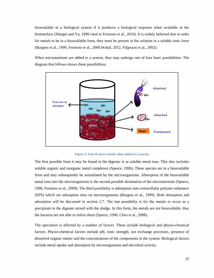
25

bioavailable in a biological system if it produces a biological response when available at the

biointerface (Shargel and Yu, 1999 cited in Fermoso et al., 2010). It is widely believed that in order

for metals to be in a bioavailable form, they must be present in the solution in a soluble ionic form

(Burgess et al., 1999, Fermoso et al., 2009,Wahal, 2012, Filgeuras et al., 2002).

When micronutrients are added to a system, they may undergo one of four basic possibilities. The

diagram that follows shows these possibilities:

Figure 3: Fate of micro-metals when added to a reactor

The first possible form it may be found in the digester is as soluble metal ions. This also includes

soluble organic and inorganic metal complexes (Speece, 1996). These species are in a bioavailable

form and may subsequently be assimilated by the microorganisms. Absorption of the bioavailable

metal ions into the microorganisms is the second possible destination of the micronutrients (Speece,

1996, Fermoso et al., 2009). The third possibility is adsorption onto extracellular polymer substance

(EPS) which are adsorption sites on microorganisms (Burgess et al., 1999). Both absorption and

adsorption will be discussed in section 2.7. The last possibility is for the metals to occur as a

precipitate in the digester mixed with the sludge. In this form, the metals are not bioavailable, thus

the bacteria are not able to utilize them (Speece, 1996, Chen et al., 2008).

The speciation is affected by a number of factors. These include biological and physio-chemical

factors. Physio-chemical factors include pH, ionic strength, ion exchange processes, presence of

dissolved organic matter and the concentrations of the components in the system. Biological factors

include metal uptake and absorption by microorganisms and microbial activity.

26

A number of studies on the metal sorption by anaerobic granules have confirmed that the extent of

sorption of metal ions are due to precipitation, coprecipitation, adsorption and binding by

Extracellular Polymetric Substance (EPS) produced by or associated with the anaerobic bacteria

(Fermoso et al., 2009). EPS is a major component of bioaggregates such as activated sludge flocs or

biofilms that binds metals (Guibaud et al., 2008). If the binding ability is high, this could reduce the

bioavailability of the metal (Fermoso et al., 2010). The strength of the bond as well as the particle

surface properties play a role in determining bioavailability (Filgueiras et al., 2002).

The bioavailability and movement of essential trace metals are greatly affected by sulphide

formation and dissolution (Van der Veen et al., 2007). The presence of sulphide, carbonate and

phosphate anions in the bioreactor greatly affect the bioavailability of the metals due to the

formation of trace metal precipitates (Speece, 1996).

A study performed by Fermoso et al. (2010) on the dosing of anaerobic bioreactors with cobalt,

showed that the chemical nature of the species of cobalt dosed strongly affected the amount of

cobalt retained in the sludge and the bioavailability. The high retention of the cobalt as precipitates

and metal ions adsorbed onto the sludge decreased the overall efficiency of the cobalt addition.

Other variables that impact the bioavailability of metals are pH (Burgess et al., 1999) and the age of

the granular sludge (Fermoso et al. 2009). Aged granular sludge has been found to reduce

bioavailability of the trace metals by reducing the dissolution rate.

Chelating agents can be used to overcome the problem of non-bioavailable forms of metals in the

bioreactors. It has been reported that microbially produced chelators have a great impact on

bioavailability as the soluble metal complexes increase the amount of soluble metals in the

bioreactor. The addition of yeast extract was found to enhance the bioavailability of nickel and

cobalt (Gonzalez-Gil et al., 2003). This is probably due to the chelating effect of the peptides and

amino acids of the yeast extract (Speece, 1996). Cysteine, also a chelating agent, provided similar

results when replacing sulphide as a sulphur source (Jansen et al., 2007). This is not the case for the

addition of strong chelating agents such as EDTA. EDTA has been demonstrated to reduce the

bioavailability due to the strong bonds formed (Callendar and Barford, 1983).

2.5 Precipitation Chemistry Precipitation is a phenomenon often exploited in industry to remove unwanted materials in a

solution. In waste water treatment, precipitation is used to remove unwanted heavy metals from the

sludge so that disposal or use in agricultural applications is safe and nontoxic. In anaerobic

digestion of industrial effluents where nutrient supplementation is required, precipitation is an

27

unwanted activity as it reduces the amount of metals in the bioavailable phase. Metals bound in a

precipitate are not bioavailable in their current form. They are however potentially bioavailable if

conditions of the liquor change whereby the precipitates dissolve and the metals become soluble.

Precipitation and dissolution are reactions which are controlled by the solubility constant, Ksp. For

the formation of a carbonate precipitate, the following reaction applies:

Where [M+] is the concentration of the soluble metal, [CO3

2-] is the concentration of the salt and

M2CO3 is the metal carbonate precipitate formed. The solubility product, Ksp, is the product of the

activities of the metal and carbonate ions in the aqueous phase. At low concentrations, the activities

are equal to the concentrations of the metal ions (i.e. the activity coefficients are equal to one). If

the product of the ion concentrations is equal to or greater than the Ksp, then the solution is said to

be saturated or supersaturated and the metal precipitate starts forming. Components that have a low

solubility product will tend to saturate and precipitate at low metal ion concentrations and thus may

prove problematic in terms of being bioavailable.

The trace metal precipitates pose a major problem as their solubility products are low, especially for

where the metals precipitate with sulphide. Callendar and Barford (1983) state that in the presence

of as little as 0.0003 mg/l of the hydrogen sulphide ion, the predicted solubilities of Fe2+

, Co2+

and

Ni2+

are 0.0000016, 0.000000006 and 0.000000004 mg/l respectively. Since the hydrogen sulphide

ion is in equilibrium with the sulphide ion (HS- ↔ H

+ + S

2-), when the concentration of HS

-

decreases, the S2-

concentration also decreases. This, in turn, causes the equilibrium metal

concentration for that Ksp to rise. Therefore the concentration of HS- has a controlling influence on

the solubility of base metals.

The table that follows provides the Ksp for certain compounds in water at 25°C (Seely, 2007).

28

Table 6: Solubility products for certain compounds in water at 25°C

Compound Formula Ksp Compound Formula Ksp

Cobalt(II) sulphide CoS 4.0 x 10-21

Cobalt(II) carbonate CoCO3 1.4 x 10-13

Copper(II) sulphide CuS 6.0 x 10-37

Copper(II) carbonate CuCO3 1.4 x 10-10

Iron(II) sulphide FeS 6.0 x 10-19

Iron(II) carbonate FeCO3 3.2 x 10-11

Nickel(II) sulphide NiS 3.0 x 10-19

Nickel(II) carbonate NiCO3 6.6 x 10-9

Zinc sulphide ZnSsp 2.0 x 10-25

Zinc carbonate ZnCO3 1.4 x 10-11

Bioavailability is more complicated than knowing the solubility products of the metal precipitates.

Jansen et al. (2007) explains that this is due to ambiguous nature of the equilibrium distribution of

the metals over their possible forms. There are a number of pertinent factors which are surrounded

by uncertainty. These include the nature and degree of crystallinity of the precipitate, the size of the

particles formed and the extent of coprecipitation and adsorption. Kinetics such as slow

precipitation and dissolution are also pertinent factors (Martell and Smith, 1989 cited in Jansen et

al., 2007). It has therefore been concluded that it is not possible to accurately predict the

concentration of the different metals in soluble form or across all possible forms of metal (Jansen et

al., 2007).

It is clear that the interactions of metals ions with other components once dosed to a system are

complex. Chemical speciation, which is the distribution of an element between its chemical species,

is an important tool for understanding these interactions. Understanding the chemical speciation is

therefore imperative as it will provide insight into the bioavailability of metals.

2.6 Methods to determine Bioavailability in a system Chemical speciation and thus bioavailability of a system may be determined using two approaches.

The first approach is an analytical approach where experimentation is performed to determine the

concentrations of the different species of metals. The second approach is using chemical speciation

modelling.

2.6.1 Analytical Approach

Most analytical approaches focus on the determination of the free metal ion concentration or the

total metal concentration. These have been well developed due to their application in assessing

29

toxicity of heavy metals in natural waters. The following is a list of analytical techniques that are

available (Nordstom, 1996; Hanrahan, 2010; Peijnenburg and Jager, 2003):

Ion selective electrodes

Voltammetric techniques (Differential-pulse polarography (DPP), Differential-pulse anodic

stripping voltammetry (DPASV))

Atomic Spectroscopy (Graphite furnace atomic absorption (GFAA), Inductively coupled

plasma mass spectroscopy (ICP-MS), Atomic emission spectrometry (AES))

X-ray spectroscopy

Neutron activation analysis

Ion exchange equilibrium (Exchange resins, Diffusive gradients in thin films (DGT),

Donnan Dialysis membranes)

Solvent Extraction

UV visible spectrophotometry

Vapour and Hydride generation

Capillary electrophoresis (CE)

All of the above techniques are used for determining the free metal ion concentration or metal

complexes in the dissolved phase. Ion selective electrodes are the most direct way of determining

free metal concentrations. With the Cu electrode, solution activities up to 10-12

M are detectable but

measurements using other electrodes are unreliable at low concentrations due to reduced sensitivity

and interferences (Sauve et al., 1995). Voltammetric as well as ion exchange techniques may be

used to determine organic and inorganic metal complexes. Care should be taken when employing

voltammetric techniques to analyze samples containing dissolved organic matter (DOM) as the

DOM may diminish current readings (Peijnenburg and Jager, 2003).

UV visible spectrophotometry and vapour and hydride generation are suitable for determining

redox species (Nordstrom, 1996). Capillary electrophoresis (CE) is a method that allows for the

direct measure of chemical species of metals. However, it is a new method and further development

of this technique is required (Hanrahan, 2010).

Direct determination of speciation in a solid sample is restricted to a few major components since

sensitivity is insufficient for trace metals (Filgeuras et al., 2002). Thus for determination of other

chemical forms such as adsorbed and precipitated metal forms, combinations of techniques are

required. Sequential solvent extraction is one such technique where solvents of increasing strength

are sequentially applied to a sample. The liquid extract from each solvent is then analysed using

30

one of the techniques described above. Extractions work on the principle that the solvent used as an

extractant solubilises the metals in a particular form (adsorbed or precipitated) and consequently it

is released into the solution (Peijenenburg and Jager, 2003). As the strength of the reagent

increases, the form of metal extracted is less bioavailable. There are a number of sequential

extraction techniques in literature with the methods proposed by Stover et al., 1976 and Tessier et

al., 1979 being the most popular.

The Stover et al., 1976 scheme fractionates metals into six phases whereas a modified Tessier

extraction scheme fractionates metals into four phases (van Hullebusch et al., 2005). All the phases

are not identical and different extractants are used to release metals from similar phases. The table

that follows gives the outline for these two schemes including the phases the metals are fractionated

into, the extractant used for that particular phase and the conditions for the extraction.

31

Table 7: Outline of Stover and Modified Tessier extraction schemes

Metal Phase Extractant Extracting Conditions

Stover: Exchangeable 1 M KNO3 20°C, shake for 16 hours

Adsorbed 0.5 M KF 20°C, shake for 16 hours

Organically Bound 0.1 M Na4P2O7 20°C, shake for 16 hours

Bound to Carbonates 0.1 M EDTA 20°C, 2X 8 hour shake

Bound to Sulphides 1 M HNO3 20°C, shake for 16 hours

Residual Strong Acids Microwave/plate

digestion

Modified

Tessier:

Exchangeable 1 M

NH4CH3COO

20°C, shake for 1 hour

Bound to Carbonates 1 M CH3COOH 20°C, shake for 1 hour

Bound to Organics and

Sulphides

30% H2O2 35°C, shake for 3 hours

Residual Strong Acids Microwave/plate

digestion

The exchangeable phase is the most bioavailable as it is the first phase to be extracted. Species in

this phase include weakly adsorbed metals onto solid surfaces via weak electrostatic forces, metals

that are released by ion exchange processes (Filgeuras et al., 2002). Salt solutions are used as

reagents since they are a source of cations. These cations displace exchangeable metals from the

sludge inorganic and organic sites (Stover et al., 1976). Alkali metals cause interferences during

atomic spectroscopy. Using the ammonium salt of the modified Tessier scheme over the potassium

nitrate in the Stover scheme is therefore advantageous (Filgeuras et al., 2002). However, the

beneficial use of nitrate salts over acetate salts is that no metal complexing occurs from the nitrate

ions and therefore metals are removed via cation exchange only (Filgeuras et al., 2002).

For the adsorbed phase in the Stover scheme, the pH and concentration of KF facilitates the

extraction of soluble metal fluoride complexes (Stover et al., 1976). There is no reagent for the

extraction of adsorbed phase in the modified Tessier scheme.

32

The organically bound metals include complexation and bioaccumulation processes with organic

matter (Coetzee, 1993). Organic matter shows a greater affinity for divalent ions than monovalent

ions (Filgueras et al., 2002). Metals in this phase are extracted by decomposition of the organic

matter through oxidation. Some oxidising reagents such as hydrogen peroxide also release metals in

sulphide precipitates, hence these are grouped together. Na4P2O7 and EDTA are both able to

remove organically bound metals due to their oxidizing and chelating abilities respectively. It is for

this reason that the organically bound extraction precedes the carbonate extraction in the Stover

scheme. This is an important fraction in sewage sludge and may dominate trace metal distribution

(Stover et al., 1976).

Metals precipitated or co-precipitated with carbonates are inclined to dissolve upon reduction of

the pH. Thus, mild acids such as EDTA and CH3COOH are used (Filgueras et al., 2002). A stronger

acid (HNO3) is used to extract metals in sulphide precipitates following the carbonate extraction.

The residual fractions are mostly extracted in the manner of determining total metal

concentrations. This is through acid digestion of the remaining solid sample using a microwave or

hot plate digestion technique according to those set out in Standard Methods (APHA, 1996).

Sequential extraction experiments performed on different sludge samples indicate although

different samples will have different distributions, the organically bound, carbonate and sulphide

precipitate and residual phases are significant with the organically bound and precipitate phases

being more significant that the residual phase (Stover et al., 1976, Filgueras et al., 2002, van

Hullebusch et al., 2005, Aquino and Stuckey, 2007). These observations have been found for Fe,

Cu, Zn, Mn, Ni and Co.

There is no uniformity between different extraction techniques as they use different solvents that

extract metals from phases which are not always comparable. This makes direct comparisons

difficult as the metal phases are defined more as a result of the operation rather than from a

universal understanding of what metal species contribute to a particular phase (Peijenenburg and

Jager, 2003). Different extraction techniques performed on the same sludge sample also produce

different distributions between the phases (van Hullebusch et al., 2005). Other problems associated

with sequential extractions are the inability of the reagents to selectively extract metals in a

particular phase and the influence of operating conditions (pH, temperature, particle size etc.)

(Filgeuras et al., 2002).

Analytical techniques are limiting in that they are not able to fully identify species of metals in all

the phases. There are also sensitivity and detection problems at trace concentrations as well as

33

interferences of certain metals with each other or with the equipment when analyzing. Another

concern is the disruption of equilibrium when sampling or analyzing occurs (Nordstrom, 1996;

Filgueras et al., 2002). Thus to determine chemical speciation, analytical methods should not be

used in isolation but should rather be coupled with chemical speciation modelling.

2.6.2 Chemical Speciation Modelling

Chemical speciation models are based on thermodynamic principles and empirically derived

constants. Total concentrations of components in the system are used to generate mass balances for

each component where the total mass of a component is equal to the sum of the mass of the

component in each of its species. These together with mass action equations for each species are

used to predict the speciation at equilibrium. There are numerous chemical equilibrium speciation

models of which Visual MINTEQ (MINTEQA2 with an updated user interface), MINEQL+ and

PHREEQC are among the popular programs. These come with standard thermodynamic databases.

Hanrahan (2010) explains that speciation models are structured such that all species within the

system can be formed by components and no components can be formed by a combination of other

components. Thus, mass balances for each component can be written as follows:

∑

Where:

Mj is the total mass of component j

Aij is the stoichiometric coefficient for the number of moles of component j in species i

xi is the activity of aqueous species i

γi is the activity coefficient of species i

N is the number of components

Mass action or equilibrium expressions can also be written as follows (Hanrahan, 2010):

∏

Where:

βi is the overall equilibrium formation constant for species i

34

cj is the concentration of component j

The equilibrium formation constants as well as a detailed explanation of equilibrium speciation

modelling equations may be found in Stumm and Morgan (1996).

Since the models are based on experimentally derived constants, they are only as accurate as the

assumptions and data on which they are based (Peijenenburg and Jager, 2003). The majority of

trace metal stability data based on experimentation have not been fully verified due to the inability

to provide evidence for certain complexes at those concentrations (Turner, 1995). The models also

have a range of applicability (those conditions at which thermodynamic data and constants were

derived) which should be adhered to.

The models are based on the local equilibrium assumption which states that since aqueous reactions

are reversible and swift when compared to other systems, they may be assumed to have reached

equilibrium (Hanrahan, 2010). This assumption can be debated as it depends on the time frame of

the system as well as the types of reactions occurring. When used to predict speciation in sediments

or mines in a time span of years, this assumption will hold. When used to predict shorter time

frames, the types of reactions that occur will determine whether this assumption holds.

Inorganic complexation reactions reach equilibrium rapidly though organic complexation reactions

are slower, especially in the presence of solid organic matter (Turner, 1995). For the adsorption of

trace metals onto solid organic matter, time is needed for the metal to become incorporated into the

solid matrix thus no true equilibrium is reached (Turner, 1995). Using analytical techniques,

Hanrahan (2010) showed that equilibrium speciation models are not suitable for predicting chelate

systems due to slow kinetics. It is suggested that reaction kinetics should be integrated into

equilibrium models for such systems.

A kinetic model for a weak acid/base system was developed by Musvoto et al., 2000. This model

takes into account the kinetics of the forward and the reverse reactions for the components included

in the model. Metal precipitation is also included in the model for compounds able to precipitate

from magnesium, calcium, carbonate, ammonium and phosphate ions. They are integrated via a

differential equation where the concentration of precipitate formed is a function of the precipitation

rate constant, the amount of precipitate formed at time t, and the amount of precipitate at

equilibrium. The model showed a good correlation when validated against equilibrium literature

values.

35

Both analytical techniques and speciation modelling have intrinsic uncertainties attached to their

usage. It has been suggested that using the methods in conjunction with each other provides a better

understanding of the system and its speciation (Nordstrom, 1996). While the use of analytical

techniques for understanding bioavailability in anaerobic sludge is common, the results of these

studies have not been verified through any kind of modelling.

2.7 Uptake of metals by the microorganisms There are two ways in which microorganisms may take up metals from solution. The first way is

through adsorption, when metals or ions bind to the surface of the microorganisms.

Microorganisms contain adsorption sites for various cations in the form of extracellular polymer

substance (EPS) as well as other sites made up of proteins and phospholipids. Extracellular

polymers include substances such as polysaccharides, proteins, RNA and DNA that contain anionic

functional groups that act as ligands. Adsorption of the metal ions onto the extracellular ligands is

said to be at a maximum when the pH is between 6.0 and 8.0 (Geradi, 1986 cited in Burgess et al.,

1999).

The second means of taking up metals is through absorption, where the metal ion is assimilated into

the cell. Simkiss and Taylor (1995) discussed the possibility of a metal entering the cell and passing

through the cell membrane, depending on the routes that are available and the form or forms that

the metal is in. There are numerous routes for a metal to be absorbed by a cell (Simkiss and Taylor,

1995). These are:

1. Through hydrophobic solution in the membrane.

2. As an attachment to the membrane proteins, lipids or carbohydrates.

3. Via endocytosis (a form of cellular ingestion where the plasma membrane folds inward to

bring substances into the cell as explained in Ivanov, 2008) of the membrane

components.

4. Permeation through water channels, non-specific channels or specific channels.

5. Permeation by general active processes (such as movement due to differences in

electrochemical potentials) or by specific active processes (such as ATPases).

Metal absorption is not possible with all the forms of metals. Permeable forms include metal ions

(M2+

), hydrated ions (M(H2O)62+

), charged metal complexes (MCl(H2O)5+), uncharged inorganic

complexes (MCl20) and organometallic complexes (CH3M

n+) (Simkiss and Taylor, 1995).

36

The transport of the metal ions relies heavily on the properties of the transport system (Braun et al.,

1998 cited in Chen et al., 2008). This may be described by Michaelis Menten kinetics, where the

metal ion is first bound to the transporter site and thereafter taken up by the cell (Fermoso et al.,

2009). Fermoso et al. (2009) stated that binding properties determine the metal-transporter

interaction while the amount of transporter determines the maximum uptake of metals. Different

metal ions may compete for the same uptake site, affecting the attraction between the metal and

transporter (Sunda and Huntsman, 1998). Another factor is the changing number of transporters by

microorganisms in response to changes in its environment (Worms et al., 2006). A reduction in the

available binding sites or the number of transporters may adversely affect bioavailability.

2.8 Micronutrient dosing

2.8.1 Dosing Strategy

Dosing of micronutrients is an offset between maximizing biological activity and minimizing costs

associated with metal losses into the environment (Fermoso et al., 2009). The technique used to add

metals to a system affects the amount of metals lost to the environment. In methanol-fed upflow

anaerobic sludge bed reactors, dosing strategies of cobalt have been investigated. Continuous

addition of a low concentration CoCl2 was compared to a pulse addition of a higher concentration,

and the specific methanogenic activity was found to be higher during the pulse dosing than in the

continuous dosing (Zandvoort et al., 2002; Zandvoort et al., 2004).

The form in which a metal enters a system also plays a role in determining its effect. In research

conducted using acetate as a substrate, Fe, Co and Ni were introduced to the system by premixing

with other components of the inorganic media, but low acetate utilization rates of 4 to 8 kg/m3 -d

were observed (Speece, 1996). The metals were then introduced by injecting the metal chloride

salts into the reactor directly. This resulted in acetate utilization rates of above 30 kg/m3 –d.

Another example is provided by Fermoso, (2008): Ni was dosed to methanol-fed UASB reactors as

NiCl2 in the one instance and NiEDTA2-

in the other instance. A higher specific methanogenic

activity was reported for the sludge dosed with the NiEDTA2-

. This was attributed to the formation

of different nickel species (such as NiS2) when free nickel was dosed to the system (upon

dissolution of NiCl2). NiEDTA2-

is less available to bonding with other ions and thus remains in its

bioavailable form.

The timing of the dosing has also been shown to produce different effects in anaerobic systems

(Fermoso et al., 2008a). In a study, cobalt addition to a cobalt-limited bioreactor that was done

before volatile fatty acid (VFA) accumulation enhanced methanogenesis however, when addition

37

occurred after VFA accumulation, an increase in the VFA concentration occurred resulting in

reactor acidification (Fermoso et al., 2009). Frequency of dosing is also an important factor to

consider. In an acetate utilization rate study, Fe supplementation one weekly was insufficient. In

order to obtain high utilization rates, Fe has to be dosed every second day (Speece, 1996).

2.8.2 Recipes Used

In literature, there are a variety of micronutrient recipes that are used to supplement anaerobic

digesters. These differ with regards to the composition, concentration and the metal salts used.

Some of the recipes are based on literature values of metal requirements for specific methanogen

strains while others are based on the elemental composition of the microorganisms. The majority of

the recipes used are not reported to be optimal for the particular system being treated.

The recipe currently used by Sasol for their anaerobic digestion process, sourced from Du Preez et

al. (1987) as cited in Van Zyl (2008) is as follows:

38

Table 8: Nutrient recipe used by Sasol for their anaerobic digestion of FTRW

Species Element Element concentration (mg/l)

FTRW (COD) COD 18 000

Urea N 250

KH2PO4 P 60

K 130

MgCl2.6H2O Mg 13

Na2SO4 S 23

CaCl2.2H2O Ca 3

FeSO4.7H2O Fe 11

MnSO4.5H2O Mn 0.2

ZnSO4.7H2O Zn 0.33

NiCl2.6H2O Ni 0.1

CuSO4.5H2O Cu 0.15

CoCl2.6H2O Co 0.02

Na2MoO4.2H2O Mo 0.007

H2BO3 B 0.009

KI K 0.001

Yeast Extract 5

A table with the recipes used in literature, is provided in Appendix A. This table provides the

metals in the recipe, their concentration, the form in which they are dosed, as well as their

comparison to the recipe above.

It is difficult to compare the recipes as the substrates, feed COD concentrations and OLR are

different. Since each system has a unique mix of microbial consortia due to their substrate,

conditions, and history, each system will have a unique recipe for optimal anaerobic functioning.

However, it was noticed that Co and Mo were metals that were dosed in significantly higher

39

concentrations in 13 and 12 of the 18 recipes respectively than in the Du Preez et al., 1987 recipe.

Another highlight is that the waste water being treated by Sasol has a very high COD (18 g/l) when

compared to the substrates of the other systems. There are only two cases where the feed COD was

higher; 118 g/l for a batch system treating alcohol distillery waste and a pH-stat reactor keeping the

pH constant with an Acetate utilization rate of 30-60 g/l. In both these cases, only P, K and Co and

Ni, Co and Ca respectively were dosed in higher concentrations. In the case of macronutrients N, P,

K and S, the recipe used by Sasol uses higher concentrations in most cases when compared to the

dosage concentrations of the other systems listed.

2.9 Anaerobic Sequencing batch reactors Bioreactor design is important for any biological process as it has an impact on the conditions

experienced by the microorganisms. It therefore has an effect on the behavior of the

microorganisms and this affects the degree of the anaerobic digestion. Burgess et al. (1999) has

stated that the bioreactor design affects the waste degrading performance as well as the way

microbes respond to the micronutrients. It is also well known that the volume of sludge produced is

a function of the bioreactor design (Chisti, 1998).

2.9.1 Sequencing Batch Reactor operation

Sequencing batch reactor operation consists of a single vessel that undergoes four different stages

of operation. These include the feeding, reaction, settling and liquid withdrawal stages (Zaiat et al.,

2001). The following diagram depicts the operation schematically:

Figure 4: Schematic representation of one cycle for a sequencing batch reactor.

40

The fill or feeding step consists of adding the wastewater or substrate to the vessel that contains the

sludge. It is best to allow the microorganisms to acclimatize to the new conditions first before

adding the wastewater as sudden and drastic changes may cause certain species of microorganisms

to die, reducing the diversity of the population. If the wastewater is applied at a high organic

loading rate, the system should be slowly acclimatized by loading in increments so as to prevent

shocks to the system.

During the reaction phase, slight agitation to the contents is provided via a stirrer. In this stage the

anaerobic microorganisms degrade the organic components of the wastewater, resulting in the

production of biogas. The stirrer maintains the contact between the microorganisms, nutrients and

the substrates, maximizing degradation. Agitation should not be aggressive as this prevents the

formation of bacterial flocs (Massé and Masse, 2000). At the beginning of this step, the food-to-

microorganism ratio is high, leading to high biogas production (Sung and Dague, 1995). The length

of the reaction step is dependent on the substrate characteristics and effluent quality requirements.

Wastewaters which have a high suspended solids concentration will require longer times for

complete hydrolysis of the complex matter to occur (Massé and Masse, 2000). The completion of

this stage is characterized by a reduction in biogas production rate.

The settling stage is initiated after the reaction is effectively complete. This permits the solids and

liquid phase to physically separate, with the solids settling at the bottom and the supernatant

collecting at the top. Settling conditions are enhanced by the equilibrium between the partial

pressure of CO2 in the head space above the supernatant and the CO2 dissolved in solution (Massé

and Masse, 2000). This step is dependent on the biomass characteristics. If the biomass is granular,

a high cellular retention in the bioreactor is achieved and this assists in attaining an improved

separation between the phases (Zaiat et al., 2001). The time taken for this stage to be completed

varies. Sung and Dague, 1995) report that typically, this ranges between ten to thirty minutes.

The clarified supernatant which forms due to settling is then drawn from the bioreactor in the last

step. Microorganisms that display poor settling characteristics are also removed (Sung and Dague,

1995).

2.9.2 Advantages and Disadvantages

Anaerobic sequencing batch reactor (AnSBR) technology provides a number of advantages over

alternative technologies. There is an improved retention of the biological solids and process control

is more advanced. Enhanced effluent quality control is achieved since reactor draw is performed

when the desired biogas emission has occurred. This is allowed due to the non-continuous nature of

41

the system. There is a high initial substrate concentration with a high biogas yield. Efficient sludge

separation is attained. There is no need for liquid or solids recycling and primary or secondary

settling is not required. The removal efficiency of organic matter is high and there is no short circuit

(as in fixed-bed continuous systems). AnSBR allows the process to be operated in a simple and

stable manner. Kinetic advantages such as a higher methanogenic activity have been reported.

(Zaiat et al., 2001). For this setup, other advantages include facilitation of overall mass balances

through batch feeding and batch effluent collection. The batch setup also allows for the collection

of gas production rate data over the entire substrate loading range in a single cycle.

There are also disadvantages when using such a technology (Zaiat et al., 2001). These include a

long settling time, a slow start-up period, solids washout, inhibition due to organic loading and a

poor understanding of agitation and feed strategy due to the developing nature of the technology.

42

3. Research Methodology

From the literature review, it was established that in order to understand the bioavailability and

speciation of a system, experimental work cannot be done in isolation due to the uncertainties and

errors involved. This study was therefore comprised of experimental work as well as speciation

modelling development.

The governing hypothesis for this study is:

A combined mass balance and speciation-precipitation model can be used to

predict soluble metal ion concentration in an anaerobic sequencing batch reactor

such that changes in methanogenic activity in response to changes in metal ion

concentration can be predicted.

Therefore the research methodology was constructed to:

1. Measure the proportions in which metal ions studied are distributed between the different

phases in anaerobic mixed liquor.

2. Develop a simple model to predict the metal ion speciation in an anaerobic mixed liquor

considering only aqueous phase association/dissociation reactions and precipitation of

selected minerals and compare this model to measurements of metal speciation in an

anaerobic reactor subjected to a major change in micronutrient dosing strategy.

3. Monitor indicators of microbial activity in an anaerobic digester in response to a major

change in micronutrient dosing strategy and attempt to identify any correlation between the

anaerobic activity and the measured and predicted metal concentrations in solution.

The investigation into microbial activity was performed using anaerobic sequencing batch reactors.

A sequencing batch reactor operates in a semi batch mode in which a typical cycle consists of

1. Feeding, where a batch of substrate is contacted with sludge,

2. A period of time for digestion of the feed (and assimilation/redistribution of metal ions),

and then a spent or treated supernatant is withdrawn either after

3. A period in which the sludge can settle

4. Allowing a clear supernatant to be withdrawn, or (iii. and iv.) through a membrane filter

without requiring a sludge settling step. (Zaiat et al., 2001).

While this configuration is rarely used in full scale processes, it has a number of significant

advantages for this type of experiment; specifically:

43

1. Batch addition and withdrawal of feed and spent supernatant allows for analysis of average

influent and effluent characteristics, thereby facilitating COD and metal mass balances over

a cycle

2. Unlike continuous processes operated under steady conditions, it is possible to observe

dynamic responses to varying food: microorganism ratios as substrate is added and then

depleted; and

3. At the end of each cycle, there is a period in which biological processes slow such that the

system can approach equilibrium with respect to liquid-gas and liquid-solid processes;

under these conditions, assumptions of equilibrium with respect to ionic speciation

chemistry may be cautiously made.

A dynamic model of ionic speciation and precipitation chemistry was developed by considering the

biological processes that took place in step 2 of a sequencing batch cycle to be a black box process

in which the end conditions after biological reactions could be calculated stoichiometrically for

complete conversion. Then from the calculated end state, the equilibrium condition of the ionic

species could be estimated by performing a speciation calculation on the anticipated total system

composition. A final mass balance calculation could then be performed to represent the change in

system composition caused by selectively removing soluble components during the decant step and

adding new soluble components with different characteristics in the subsequent feed step. Both the

biological experiment design and the model structure are described in detail in Sections 3.1 and 3.3.

Two experiments were performed, the first being a preliminary study on two existing reactors fed

on glucose and ethanol separately. The main purpose of this was to gain information regarding the

analytical methods used to determine metal speciation and concentrations. The second experiment

included running reactors on FTRW as a substrate. Information gathered from the operation as well

as results of the first experiment, experiment A, were applied to the second experiment, experiment

B to improve its operation and results.

Joint mass balance and chemical speciation modelling was performed for both Experiment A and B

in order to gain a better understanding of the dynamics of the system. The experimental work from

A when compared with the speciation modelling for A was designed to reveal the extent to which

the model is able to predict the metal distribution observed experimentally. The metal analysis and

monitoring of reactor and microbial parameters of Experiment B, together with the speciation

modelling was to be used for assessing whether speciation modelling may be used to predict

changes in microbial activity due to changes in metal concentration.

44

3.1 Experiment A Experiment A was performed on existing reactors that were being operated by other students for

different research purposes. Experiment A was mainly focussed on exploring metal speciation and

its facets. Consequently, data collection was limited to data which was in line with the objectives of

this experiment. The following is a list of objectives for this experiment:

To gain a better understanding of metal speciation when metals are dosed to a system that

contains sludge.

To ascertain whether all metals in the system, no matter where they reside, may be

accounted for.

To test the effectiveness of sequential extraction as a means to separate metals into their

respective phases.

To compare the amount of metals extracted from the sludge using different techniques, to

compare the sum of sequentially extracted metals to the total metals measured using total

sample digestion with acid, thereby investigating the reliability of each method.

To extract any lessons from the experimental methods used and apply these to Experiment

B to minimise experimental error.

3.1.1 Experimental setup

Two existing anaerobic sequencing batch reactors (ASBRs), each with identical operating

conditions but different substrates, were operated concurrently. The first reactor was fed with a

glucose substrate (brewery sludge which has been fed on a glucose solution and micronutrients for

3 months) while the second reactor was fed with an ethanol substrate (brewery sludge which has

been fed on an ethanol solution and micronutrients for 3 months). The following diagram provides

a description of the setup of one of the reactors:

45

1

2

Biogas sampling

point

Gas flow meterSignal to computer

Feed and

withdrawal line

Valve

Nitrogen line

Temperature

sensor

pH probe

Water Bath

Peristaltic

Pump

Reactor

Magnetic

Stirrer

Water Jacket

Biogas line

pH meter with thermocouple

Figure 5: Experimental setup of one reactor for Experiment A.

Each reactor was a cylindrical, 6.5 Ɩ vessel; 4.5 Ɩ was used as the working space and the remaining

volume formed the headspace. Each reactor was air-tight and surrounded by a water jacket for

maintaining the temperature of the bioreactor at 35 °C. Water from a heated water bath was

pumped using a peristaltic pump through to the water jacket as a means of heating. The reactors

were positioned on a magnetic stirrer to allow for even metals and substrate distribution.

For the addition of sludge, nutrients and wastewater, a feed line was present at the top of the

bioreactor. This was also used to withdraw the supernatant once a cycle had been completed. This

was achieved by increasing the pressure in the headspace through the addition of nitrogen gas from

the nitrogen supply line. A pipe open to the headspace above the supernatant allowed the biogas

produced to flow to a sampling point and a gas mass flow meter. A pH probe and a temperature

sensor connected to a pH meter with a thermocouple were located within the bioreactor. Values for

these parameters were logged on an attached computer through a data logging system.

46

3.1.2 Reactor Operation

At the beginning of operation, both reactors were inoculated with industrial brewery sludge that

was granular in nature. The bulk of the sludge solids remained in the reactors for the entire period

of operation; it was not decanted from the reactors at any stage. The reactors were run for

approximately three months before metal analysis were performed. The concentration of metals in

the sludge, feed and withdrawn supernatant streams over two complete adjacent operating cycles

for each reactor were determined. The first cycle (i) spanned four days and the second cycle (ii)

spanned three days. The ASBRs were operated at conditions pertinent to the research for which

they were constructed for (i.e. not for anaerobic digestion of high strength FTRW). Both cycles

were operated with identical conditions for feeding, reacting, settling and decanting. The following

table summarizes the operating conditions for each bioreactor:

Table 9: Operating parameters for each sequencing batch reactor

Operating Parameter Value

Total Cycle Time 4 days (cycle (i)) 3 days (cycle (ii))

Settling time 60 minutes

Fill time 30 minutes

Decant Time +- 15 minutes

Feed volume 1 Ɩ

Volume decanted per cycle 1 Ɩ

3.1.3 Influent Composition

The feed for both reactors were prepared on the day of decanting and feeding. Reactor I was fed on

a substrate of glucose while Reactor II was fed on ethanol. Sodium bicarbonate (NaHCO3) was

used as a buffer for maintaining the pH within a desirable range. The following table displays the

feed composition for both the reactors:

47

Table 10: Influent Composition for Reactors I and II, Experiment A.

Parameter Reactor I Reactor II

Feed substrate Glucose solution Ethanol solution

Feed composition (1 Ɩ feed):

-Substrate

-Nutrient medium solution

-Buffer

0.0278 mol glucose

5 mƖ

0.0298 mol NaHCO3

5mƖ ethanol (95% purity)

5 mƖ

0.0298 mol NaHCO3

Feed volume 1 Ɩ 1 Ɩ

The nutrient medium solution used was that proposed by Owen et al, 1979. A concentrated stock

solution of nutrients was prepared and a constant volume of the solution was added for each cycle

according to the desired nutrient concentrations in the feed. The stock solution only contained

macro- and micronutrients while the organic substrate and alkalinity were measured and dosed for

each cycle. The following table shows the compounds used to prepare the solution as well as the

concentration of the metals in the feed solution:

Table 11: Nutrient medium solution as proposed by Owen et al, 1979.

Compound Metal

Concentration of metal in

the feed (mg metal/ Ɩ)

(NH4)2HPO4 P 0.094

CaCl2.2H2O Ca 0.341

MgCl2.6H2O Mg 1.076

KCl K 3.410

MnCl2.4H2O Mn 0.028

CoCl2.6H2O Co 0.037

H3BO3 B 0.005

CuCl2.2H2O Cu 0.005

Na2MoO4.2H2O Mo 0.005

ZnCl2 Zn 0.005

FeCl2.4H2O Fe 0.520

The operation of the reactors, the preparation of the feed as well as the preparation of the nutrient

medium solution was performed by students conducting the external research.

48

3.1.4 Sampling and Analytical Techniques

The reactors were operated using the conditions described above. Two consecutive cycles were

chosen to perform metal analysis. Prior to this, the reactors were operated for approximately three

months; this was sufficient time to allow for startup, acclimatization and for the reactors to reach a

pseudo-steady state. The pseudo-steady state implies that at the end of each cycle, the conditions in

the reactor (metal, sludge and substrate concentrations, pH, PCO2, alkalinity and any other indicators

of process conditions and stability) returned to the same value as at the end of the previous cycle.

In an overall metal mass balance of a cycle, there are four sources/sinks of metal ions. These are the

feed, the supernatant that is decanted after each cycle and the sludge within the reactor at the start

and at the end of each cycle. Depending on whether the component was liquid or a combination of

liquid and solid matter, the samples were subjected to three different types of metal analyses:

1. Clear liquid sample: direct metal analysis was performed on a sample that was in a liquid

form and where no chemical preparation was required to extract metals from the solid form.

Samples were analyzed using Inductively Coupled Plasma- Atomic Emission Spectroscopy

(ICP-AES) to determine the metal concentration for that sample.

2. Complete or partial solid sample: A sample was subjected to acid digestion, the second

means of metal analysis, when in a complete or partial solid form (such as sludge) and

where the total metal concentration is desired. The acid digestion converted the sample into

a form (soluble) where ICP-AES could be performed.

3. Sequential solvent extraction: The last type of metal analysis performed was a sequential

solvent metal extraction. This was performed on a solid sample where the concentration of

metals residing in different phases is desired. The solvent used to extract metals in a

particular phase was analyzed using ICP-AES analysis.

Since the ICP-AES analysis provides a concentration of the sludge or supernatant sample, the mass

of feed, sludge and supernatant was required to calculate the total metal content in each of those

portions. The feed and supernatant was assumed to be equal to 1 kg, equivalent to the mass of 1

litre of water. The mass of sludge was found using the superficial density of settled sludge by

allowing the sludge sample to settle and the volume of settled sludge calculated using the level of

sludge and the reactor inner diameter. The level of sludge was not measured every cycle but rather

was found using the level of sludge measured in the first cycle and subtracting the equivalent height

of sludge lost due to sampling at each successive cycle.

49

3.1.4.1 Direct Metal Analysis

Direct metal analysis was performed on samples that were in a form capable of undergoing ICP-

AES analysis without any chemical manipulation. Inductively Coupled Plasma-Atomic Emission

Spectroscopy (ICP-AES) is a technique used to determine the composition and concentration of

elemental species in a chemical system. This works on the principle that atoms emit

electromagnetic radiation as they move from an excited state to their ground state. The radiation

emitted can be detected easily when it is in a vacuum ultraviolet, ultraviolet, visible or infrared

region. There are three general steps involved and these are atom formation, excitation and

emission. ICP-AES uses plasma for the atomization and excitation steps (Manning and Grow,

1997).

A brief method of analysis was given by Environmental Protection Agency (Martin et al., 1998).

Analysis started with weighing and measuring a sample for analysis. Sample preparation included

filtering the sample through a filter paper with 0.45 µm pore size diameter. This was done in order

to prevent blockages from occurring within the tubing or at the exit of the nebulizer spray. The

sample was pumped through a nebulizer using a peristaltic pump and then transported to the plasma

torch. Element specific emission spectra were dispersed by a grating spectrometer and the

intensities of the line spectra at specific wavelengths were monitored by a photosensitive devise.

Currents from the device were then processed by a computer system and values were reported in

mg or ppm per litre.

A Perkin Elmer Optima 5300 DV instrument, property of the UKZN School of Chemistry and

Physics, was used for the ICP-AES analysis. Since the instrument belonged to an outside party, the

settings of the instrument could not be changed. Prior to sample analysis, a calibration, using

prepared solutions of known metal concentrations, was performed. The prepared solutions, when

analysed, provide a calibration graph which is used as a basis to determine sample concentrations.

The standard solutions were prepared in a range within which sample concentrations were expected

to occur. Only sample concentrations found to occur within the range of the calibration curves were

considered valid. Preparation of the standard solutions used for calibration as well as the sample

preparation was performed internally. More details regarding the procedure of the ICP-AES

analysis as well as standard preparations, calibrations and uncertainties are provided in Appendix

B.

The feed for both the reactors were analyzed for metal content using ICP-AES since the feed was

soluble for both reactors in Experiment A. This represents metals entering the system at the start of

50

each cycle. The amount of metals determined experimentally using the ICP-AES analysis was then

compared to the theoretical concentrations calculated from the Owen et al (1979) recipe.

Since the supernatant from each cycle contained some sludge particles, it was necessary to find out

the fraction of metals lost through each phase. Filtration was required before it could be analyzed

using ICP-AES.

3.1.4.2 Acid Digestion

Acid digestion is a means to extract metals out of a solid phase through the addition of reagents

such as acids or oxidizing agents. The reagents digest the solid particles and release metals into the

liquid phase. The resultant liquid phase with the extracted metals undergoes ICP-AES analysis to

determine the metal concentration. Acid digestion may be performed using a microwave digestion

or hot plate refluxing. Both these methods are presented in the Martin et al (1998). Based on the

equipment available in the laboratory at that time, hot plate refluxing was employed. This

corresponds to method 3050B (APHA, 1996).

For each cycle, samples were obtained from the initial and final sludge within the reactor. The

samples were subjected to hot plate acid digestion to provide the total metal concentration initially

in the system and at the end of a cycle. Decants from each cycle contained a fraction of sludge

particles. These were consequently acid digested so that the total metal amount lost through the

supernatant could be established. The experimental method for the acid digestion together with an

explanation of how the sludge samples for the acid digestion were obtained is presented in

Appendix B.

By determining the total metal content in the reactor at the start and at the end of a cycle, a metals

mass balance could be performed for each cycle for both reactors. Assuming a pseudo steady-state,

for each element, the total mass of the metals entering the system should be equal to the total mass

of metals leaving the system. The following diagram shows a reactor at the start and end of a cycle:

51

Start of Cycle End of Cycle

Feed

Initial Sludge Final Sludge

Supernatant

Figure 6: Metals mass balance for a reactor for one cycle.

The dashed line from the figure above shows the boundary of the mass balance. The following

equation displays the mass balance for the system:

(2)

This mass balance provides an indication of where the metals are residing relative to the other areas

and whether all the metals in the system may be accounted for.

3.1.4.3 Sequential Extraction

The sludge samples were also subjected to a sequential solvent extraction procedure. This provides

insight into the different forms the metals occur in, and thus gives an idea of the bioavailability of

the metals in the sludge. The procedure recommended by Stover et al, (1976) (as discussed in

section 2.6.1) was used. Reagents KNO3, KF, Na4P2O7, EDTA and HNO3 were used to sequentially

extract metals in the exchangeable (through ion exchange reactions), adsorbed (by forming metal

fluoride complexes), organically bound (through oxidation of organic matter), carbonate precipitate

(through the addition of a mild acid which dissolves the precipitate) and sulfide precipitate (through

the addition of a stronger acid which dissolved the precipitate) forms respectively. The table below

summarizes the conditions of the extraction:

52

Table 12: Stover Scheme overview

Wet sludge samples were used so that a soluble fraction could be extracted. This also prevented

additional uncertainties or errors that are possible with each additional experimental step. Before

extracting the exchangeable phase, the sludge samples were centrifuged to determine the soluble

metals in that sample. Between extracting each phase, the sample and solvent were centrifuged first

and then filtered to separate the phases. The liquid phase was diluted to 50 ml using distilled water

and then analyzed using ICP-AES analysis. The volume used for dilution was taken into account

during the calculation for the amount of metal in the sample. The solid phase (including interstitial

water) was then recovered (from the centrifuge tubes as well as the filter paper) using the solvent

for the next phase.

Residual metals were found by taking the sample after extraction and placing it into a 550°C

furnace for 1.5 hours. HCL was then used to extract the metals by soaking the ash in the acid and

filtering it before using ICP-AES analysis. A more detailed experimental procedure is presented in

Appendix B. After ICP-AES analysis of the samples, the concentrations that were found were used

to find the mass of metals within the sludge using the sludge volume. The mass of metals found

within each of the phases were then summed to provide a total mass of each metal and this was then

compared to the mass found using the acid digestion method.

3.2 Experiment B Experiment B formed the main part of this investigation as it entailed experimentation on reactors

treating FTRW. Lessons learnt from the results and operations of Experiment A were applied to

Experiment B. During the experimental work for A, a number of errors were encountered.

Consequently, for experiment B, steps were taken to eliminate these errors. Experiment B was also


Exchangeable 30 mƖ, 1 M, KNO3 20°C, shake for 16 hours

Adsorbed 48 mƖ, 0.5 M, KF 20°C, shake for 16 hours

Organically Bound 48 mƖ, 0.1 M, Na4P2O7 20°C, shake for 16 hours

Bound to Carbonates 48 mƖ, 0.1 M, EDTA 20°C, 2X 8 hour shake

Bound to Sulphides 30 mƖ, 1 M, HNO3 20°C, shake for 16 hours

53

geared more towards verifying and finding correlations with the mass balance-chemical speciation

modelling than to provide independent data for analysis.

Experiment B entailed three parts. The initial startup and operation of the reactors, a period of

relatively stable operation and thereafter a washout experiment.

The washout experiment was performed as a step change in metal loading (either up or down) was

required to obtain a measurable change in metal concentration in one or more of the phases of the

sludge. It was also desired to see an influence of this step change on the biological activity. The

washout experiment posed as an extreme step change that allowed one to observe the extent of

leaching from the solid phase with each cycle. Since the sequencing batch reactor design was used,

an indication of the partition coefficient between the liquid and the solid phase was also possible.

Simultaneously, the effect on biological activity was observed as a significantly negative condition

for the biological process was imposed. This allowed for a possible investigation into the

mechanisms (on a macro scale, not on a biochemical scale) responsible for poor biological

performance as a result of micronutrient deprivation.

3.2.1 Experimental Setup

Two ASBRs with identical operating conditions were run concurrently. This provided a duplicate

set of results for verification purposes. The experimental setup was similar to that of Experiment A

with the exception that a peristaltic pump was used to pump the reactor contents around, in order to

provide mixing. The following picture shows the setup of the reactors:

54

Figure 7: Experiment B reactor setup

Each reactor was a cylindrical, 9 Ɩ vessel; 8.5 Ɩ was used as the working space and 0.5 Ɩ formed the

headspace. The reactors were taller than those employed in Experiment A. This was due to an

allowance made for future installments of membrane filters in the reactors as reports from plant

personnel suggested that sludge treating FTRW becomes dispersed and consequently is difficult to

settle.

Each reactor was air-tight and surrounded by a water jacket for maintaining the temperature of the

bioreactor at 35 °C. Water from a heated water bath was pumped to the water jacket as a means of

heating. The reactors were not mixed using magnetic stirrers; the previous experiments showed that

55

these were problematic. Stirrer bars tended to settle on the side of reactors, resulting in poor, and

often, no mixing. A peristaltic pump was used to obtain the required mixing of the reactor contents.

Sludge was transported from the bottom of the reactor via tubes connected to the pump to the top of

the reactor, just below the liquid level. Two dedicated pipes were used for this purpose. One pump

with two pump heads was used for both the reactors.

The inclusion of a peristaltic pump did not just aid mixing; it was also used for decanting and

feeding. A movable pipe attachable to the pump was used to decant supernatant at the end of a

settling stage. The height was adjusted according to the desired decant volume. This method of

decanting proved much more accurate than the method used in Experiment A. In A, a nitrogen gas

buildup was required to force out the liquid. This did not result in a smooth outflow of decant, thus

reducing the accuracy of volume decanted. In B, feed was introduced into the system through the

pipe that was also used for sucking up sludge from the bottom of the reactor with the exception that

the flow was reversed. This is indicated by the “Pump around Inlet” as shown in the figure below.

By introducing the feed at the bottom of the reactor a better dispersion of the feed was achieved.

56

Figure 8: Lid configuration for reactors I and II in Experiment B.

A biogas outlet pipe, as indicated above, open to the space above the supernatant was used to allow

the biogas produced to flow to a sampling point and a gas flow meter. The sampling point was used

for taking samples to find the composition using a gas chromatograph. A pH probe and a

temperature sensor were connected to a pH meter with a thermocouple located within the

bioreactor. Values for these parameters as well as the value for biogas production were sent to a

computer where values were logged constantly through a data logging system. In this way, these

parameters were monitored continuously and in real time. The nitrogen line was used to flush the

reactors once feeding was completed. This re-established the anaerobic atmosphere within the

reactors.

3.2.2 Seed sludge source

FTRW has a relatively constant composition. In a continuously fed reactor, a microbial consortium

specially adapted to the sludge will develop. Therefore to avoid a lengthy acclimatization period, a

pre-acclimated sludge was used. Two upflow anaerobic sequencing batch (UASB) reactors were

“ “

“ “

57

operated for this purpose. They also provided a uniform seed sludge source when necessary. One

UASB was originally seeded using municipal sludge from a local wastewater treatment plant while

the other initially contained industrial sludge from a beer brewery effluent treatment plant. Small

dosages of FTRW were introduced into the system and gradually increased. The microbial

organisms were acclimatized up to a concentration of approximately 2000 mg COD/Ɩ of FTRW in

the UASB reactors which corresponded to a feed concentration of 9000 mg COD/Ɩ. Operation of

the UASB reactors was performed by a post-doctoral student.

Acclimatization thereafter was performed within the ASBR to get the FTRW concentration in the

feed to 18 000 mg COD/Ɩ. A comprehensive vitamin and nutrient supplement was provided

consistently to the UASB reactors to aid in the acclimatization process.

A mixture of the industrial and municipal acclimatized sludge was used in both the reactors. The

total volume of mixed sludge in each of the ASBRs was 3.5 Ɩ. The reactors were fed without being

decanted until the working volume was 8.5 Ɩ.

3.2.3 Initial operation

During the initial operation of the reactors, the feed FTRW concentration was incrementally

increased from 9000 mg COD/ Ɩ to 18 000 mg/ Ɩ by increasing the volume of FTRW in the feed.

The concentration of the buffer, sodium bicarbonate, was also varied to keep the reactor pH within

the optimal range. This concentration did not neutralize the feed but accounted for delayed effects

from biological processes that would raise the pH. Behaviour from the previous cycle towards a

dosage of buffer was used to determine the next cycle’s dosage by observing the time taken for the

reactor pH to stabilize above a pH value of 7. This was done to prevent the disruption of a cycle by

adding a NaHCO3 solution during the cycle.

The seed sludge contained a considerable amount of vitamins and metals through the UASB

nutrient supplement dosing. During initial ASBR operation, metals were dosed according to the

Sasol nutrient recipe (Section 2.8.2). Vitamin dosing was thus omitted as it does not feature in the

Sasol recipe, and thus was not in the scope of this study. However, the effect of vitamins on the

digestion process and speciation dynamics should be pursued at a later stage.

3.2.4 Stable Operation

The initial cycles were performed until a reasonably stable operation was achieved where similar

biogas production and pH responses were observed in subsequent cycles. The influent COD

concentration was constant at 18 000 mg/Ɩ and metals were dosed consistently according to the

58

Sasol recipe. Once stable operation was achieved, the washout experiment was started. The

following table displays the influent conditions during stable operation:

Table 13: Influent Composition for ASBRs, Experiment B.

Component Concentration in Feed (mg/Ɩ)

FTRW 18 000

Buffer (NaHCO3) 5 g/Ɩ

Macronutrients According to the Sasol recipe

Micronutrients According to the Sasol recipe

3.2.5 Washout Experiment

The washout experiment entailed feeding the microorganisms as during stable operation with the

exclusion of the addition of micronutrients (Mg, Ca, Fe, Mn, Zn, Ni, Cu, Co and Mo).

Macronutrients (N, P, K and S) were still added as these are essential to the microbes and a lack

thereof would cause the reactors to fail before observing any effects due to a micronutrient

limitation. This ensured that influence of micronutrient limitations could be observed. The washout

experiment fulfilled a number of functions. These included:

To provide an extreme step change in metal loading which would result in a measurable

change in metal concentration in one or more of the phases of the sludge.

To provide an indication of the extent of leaching from the solid phase with each cycle.

Investigating the different rates of washout for the different metals.

Observing the effects of washout of metals on the biological activity of the

microorganisms.

Investigating the mechanisms (on a macro scale) responsible for poor biological

performance as a result of micronutrient deprivation.

Providing a means to validate the speciation modelling of this study.

3.2.6 Reactor Operation

The ASBRs were operated concurrently. This provided a duplicate set of results for verification

purposes. Each cycle lasted 48 hours with different feeding, settling and reaction times as in

Experiment A. The table that follows displays the operating conditions for the ASBRs.

59

Table 14: Operating parameters for the ASBRs, Experiment B.

Operating Parameter Value

Total Cycle Time 48 hours

Settling time 14 hours

Fill time 10 minutes

Decant Time 10 minutes

Feed volume 1 Ɩ

Volume decanted per cycle 1 Ɩ

Hydraulic Retention Time 17 days

It is noticeable from the table above that the settling time is unusually high. This was due to the

dispersed characteristics of the sludge. The industrial sludge is granular in nature while the

municipal sludge forms flocs of varying size. Due to the constant exposure to FTRW, the sludge

became highly dispersed and it was difficult to settle. Ideal operation of this type of sludge

necessitates a membrane filter which negates the need for settling. It is thus recommended for

future experimentation using this type of sludge to make use of a membrane reactor.

Fill and decant times were consistent due to the use of the peristaltic pump. Both reactors were

flushed for 5 minutes with N2 after feeding to re-establish the anaerobic environment within the

reactors. After flushing, the peristaltic pumps were started to provide mixing of the influent with

the reactor contents. The speed was gradually increased from 0 to 80 rpm within the first 5 minutes

of operation.

It was anticipated that micronutrient limitation would affect microbial activity in a number of ways,

including a reduction or cessation in the rate of biological processes. It was not anticipated that it

would be possible to directly determine what type of specific effects take place; however, general

effects on the system such as changes in CO2 and CH4 production rates as a result of changes in

CO2 and CH4 producing processes can be expected. It was also anticipated that the overall

microbial community’s ability to buffer against pH changes would change. Therefore, parameters

such as minimum pH, time taken for the reactor pH to stabilize above a pH value of 7 and

maximum CH4 and CO2 compositions were monitored.

60

The experiment could have been conducted either with a variable (responsive) alkalinity dosing

strategy or a fixed alkalinity dosing strategy. The varying strategy modifies the amount of alkalinity

dosed to maintain some measure of pH buffering stability. In this way, changes in reactor

conditions due to poor pH buffering are not dominant factors. Therefore, the varying strategy was

employed and implemented by monitoring the time taken for the reactor pH to stabilize above a pH

value of 7 in a cycle and adjusting the alkalinity dosage for the following cycle when the pH

stabilisation time exceeded a threshold value of 4 hours; i.e. If the time taken for pH stabilization

was over four hours, the alkalinity dosage for the next cycle was increased by 0.5 g of NaHCO3.

3.2.7 Sampling and Analytical Techniques

There were numerous parameters that required measuring and monitoring. These may be classified

into parameters relating to the system and those associated with the three different phases of the

digester, namely the biogas, supernatant and sludge.

3.2.7.1 System variables- Temperature and pH

The temperature and pH of the digester was continuously monitored using a pH meter (Honeywell

model 51453503-506) with a temperature sensor connected together with a data logging interface

built in Labview. This allowed for real time measurements to be observed. Since pH provides an

indication of the state of the system, this variable was monitored constantly.

3.2.7.2 Biogas phase

Biogas production and composition is a good indication of biological activity. The flowrate was

continuously monitored and logged in real time using a flow meter connected to data logging

technology. A sample of the biogas was extracted from the headspace of the reactor using a gas

tight syringe, via a sampling point. This was performed at regular intervals during the first five

hours of operation. Component analysis was done using a gas chromatograph (GC), model

GOWMac 350, equipped with a thermal conductivity detector. The GC was calibrated to quantify

nitrogen, carbon dioxide and methane. The following table provides the specifications of the GC

used.

61

Table 15: GC Specifications

Model GOWMac 350

Detector Thermal conductivity detector

Carrier Gas He

Flow rate (ml/min) 40

Column Hayesep D (4m x 3.2 mm OD)

Column Temperature (°C) 80

Detector Temperature (°C) 95

Injection port Temperature (°C) 95

Current (mA) 100

3.2.7.3 Supernatant Analysis

The supernatant was decanted after selected cycles for reactor I and reactor II and was analysed for

metal content using ICP-AES. The samples were first filtered using a 0.45 µm pore size filter paper

to eliminate solid particles that would interfere with the analysis. All samples were prepared in the

laboratory and thereafter taken to UKZN Westville Campus to the analytical laboratory in the

School of Chemistry and Physics for analysis.

The supernatant samples in experiment B were not subjected to acid digestion as the solid content

in the effluent was substantially lower than the solids lost through the decant in Experiment A. Any

solids lost through decanting were calculated by subtracting the metals from the filtered supernatant

ICP-AES analysis from the total metals found from the acid digestion of the sludge.

3.2.7.4 Analysis of the sludge

In Experiment B, sludge samples were collected at the end of each cycle after decanting. Before

sampling, the sludge within the reactors was mixed using the pumps and samples were drawn from

the bottom of the reactor. For selected cycles, the samples were subjected to acid digestion. This

provided an indication of the total amount of metals within the reactor before and after a particular

cycle. Samples were not subjected to sequential extraction. The chief reason for this was the

significant experimental errors encountered during the process for Experiment A (Section 4.1.3).

62

3.3 Mass Balance-Chemical Speciation Modelling

3.3.1 Rationale

Due to the uncertainties with using only experimental techniques for determining metal speciation

in an anaerobic system, it is recommended that speciation be determined using modelling.

Modelling can continue to predict trace metal concentrations at values below the detection limits of

the available analytical techniques, although the results at these concentrations are by definition not

directly verifiable. Nevertheless, the model may provide some clues as to which mechanisms may

be active in the dynamics that are observable. For a dynamic anaerobic system, there is as yet no

model in the literature to mechanistically represent metal speciation in a mixed system. Thus the

development of such a model should be highly beneficial. Using existing tools to develop the

dynamic system was a good starting point.

Multiple chemical equilibrium speciation models exist, Visual MINTEQ (VM) being the most

accessible as well as well-established and well-validated. VM provides equilibrium results however

this research aims to represent a dynamic system. It was decided to use VM, but in such a way

where each model simulation together with a mass balance performed in Microsoft Excel

represented one anaerobic sequencing batch cycle. By performing multiple runs of the combination

of VM and mass balances, the way the system changes with progressing cycles may be seen.

The choice of utilizing an ASBR system for experimental work is paramount as the batch method

allows for each cycle to reach a quasi-steady state such that equilibrium of the liquid, and to a

certain extent, solid phases, may be assumed. The feeding and decanting stages in the ASBRs are

catered for by the mass balance equations while reacting and settling times are modelled using VM.

This would be difficult if not impossible for continuous systems such as the continuous upflow

anaerobic sequencing batch reactors since their operation, although able to reach a steady state, may

not reached a point in its operation that is close to ionic equilibrium.

3.3.2 Model Development

Due to the complexity of the system and the novel nature of the model, the approach used in the

development was a stage-wise approach. The model was therefore defined in the simplest way

possible, with metals existing in only a soluble (free ion) phase or in a metal precipitate. However,

the long term objective of this research is to extend the model to more complex forms, where the

simplifying assumptions in a simple model are not justified by the data.

63

3.3.2.1 Initial Conditions

In order to initiate the model, initial conditions were chosen. An existing model of anaerobic

digestion of FTRW developed using WEST for a continuous membrane reactor (Van Zyl et al.,

2012) was used to estimate the starting inorganic species concentration in the ASBR. Thus this

would provide satisfactory initial conditions for all species except for metals as these are excluded

from the Van Zyl model. Initial conditions for the model were determined by selecting reactor

volumes and feed concentrations pertinent to this study. Since the WEST model was developed for

a continuous system, a feed flow rate equivalent to the volume of feed per cycle divided by the

cycle time was used. The simulation was performed by another postgraduate student and the output

from WEST was used to represent the reactors before feeding (Lees, 2013). Therefore, the initial

conditions used as an input to VM were the output concentrations from WEST plus the reactor feed

concentrations.

It was anticipated that the mass balance speciation model would tend to an inorganic species

equilibrium that was independent of the initial conditions. However, the selection to use the WEST

model was based on a desire to begin with values as close to the actual conditions in the reactors as

possible. It was believed that the WEST model gave the best available estimate for these. The tables

containing the initial conditions for the models of both experiment A and B are contained in

Appendix D.

3.3.2.2 Settings

When using VM, the default setting for allowing precipitate formation is off. For each cycle, for the

speciation modelling, a VM run where no solids were allowed to precipitate was first performed.

From the results, all the possible precipitates were those compounds with a saturation index (SI) of

greater than one. A run thereafter was performed where solids were allowed to precipitate.

However, not all precipitates with SI of greater than one will precipitate under the conditions of the

experiment. Therefore a review of all supersaturated minerals was performed to identify which

might precipitate during an experiment (Section 3.3.3). The second run provided the results for the

speciation modelling.

3.3.3 Assumptions

During the development of this model, certain assumptions had to be made. Due to the novel nature

of this steady-state mass-balance model, it was decided to begin with a simple model as a basis

which may be built upon at a later stage. For this reason, many simplifying assumptions were made,

64

some of which may be questionable in other scenarios. The following list provides these

assumptions:

1. At the end of each cycle, the system and its reactions reach a state of equilibrium.

2. Growth of microorganisms did not affect the concentrations of the ions.

3. The increase in mass of the sludge due to bacterial growth was 10 g wet sludge and was

equal to the mass of sludge lost during decanting.

4. The electrical potential and reduction/oxidation reactions of the system were not taken into

account.

5. Metals may be found as free or complex inorganic soluble ions in solution or in a solid

precipitate form. Metal adsorption and the formation of organic complexes were not

accounted for.

6. The pH of the system was not an input into the model; it was determined by the VM

speciation calculations.

7. Only certain precipitates were allowed to form. Table 15 that follows provides a list of all

the potential precipitates according to VM, i.e. minerals that were predicted to be

supersaturated at the end of the ASBR cycle, whether they were allowed to precipitate or

not and the reason/s for that decision.

8. The precipitates that were formed during the VM modelling are only lost via the sludge. It

is assumed that the amount of precipitates lost via the supernatant was 0.3% of the volume

of sludge lost.

9. For the setup of Experiment A, the partial pressure of both CH4 and CO2 for the glucose-

fed reactors was 0.5 atm. For the ethanol-fed reactors, the partial pressures were 0.65 atm

for CH4 and 0.35 atm for CO2. These were based on the following equations:

For Glucose:

For Ethanol:

10. For the setup of Experiment B, the partial pressures of CH4 and CO2 that were used

corresponded to the average values determined experimentally. These partial pressures

were 0.72 and 0.28 atm for CH4 and CO2 respectively.

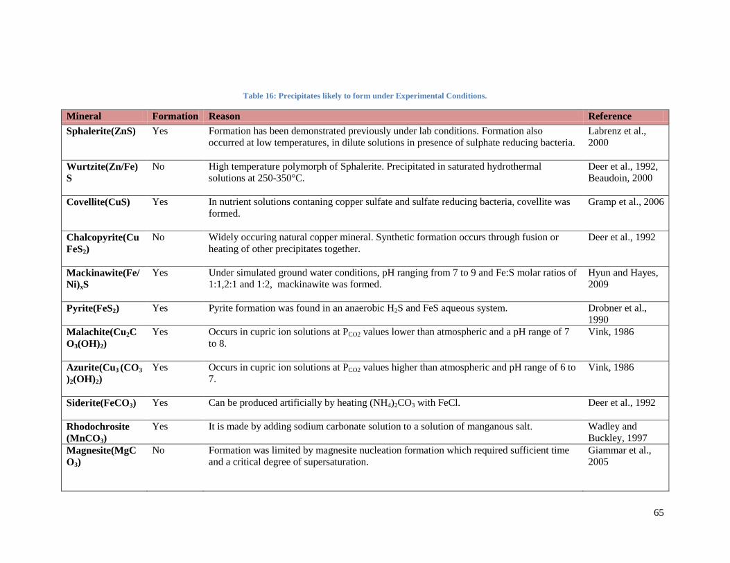
65

Table 16: Precipitates likely to form under Experimental Conditions.

Mineral Formation Reason Reference

Sphalerite(ZnS) Yes Formation has been demonstrated previously under lab conditions. Formation also

occurred at low temperatures, in dilute solutions in presence of sulphate reducing bacteria.

Labrenz et al.,

2000

Wurtzite(Zn/Fe)

S

No High temperature polymorph of Sphalerite. Precipitated in saturated hydrothermal

solutions at 250-350°C.

Deer et al., 1992,

Beaudoin, 2000

Covellite(CuS) Yes In nutrient solutions contaning copper sulfate and sulfate reducing bacteria, covellite was

formed.

Gramp et al., 2006

Chalcopyrite(Cu

FeS2)

No Widely occuring natural copper mineral. Synthetic formation occurs through fusion or

heating of other precipitates together.

Deer et al., 1992

Mackinawite(Fe/

Ni)xS

Yes Under simulated ground water conditions, pH ranging from 7 to 9 and Fe:S molar ratios of

1:1,2:1 and 1:2, mackinawite was formed.

Hyun and Hayes,

2009

Pyrite(FeS2) Yes Pyrite formation was found in an anaerobic H2S and FeS aqueous system.

Drobner et al.,

1990

Malachite(Cu2C

O3(OH)2)

Yes Occurs in cupric ion solutions at PCO2 values lower than atmospheric and a pH range of 7

to 8.

Vink, 1986

Azurite(Cu3 (CO3

)2(OH)2)

Yes Occurs in cupric ion solutions at PCO2 values higher than atmospheric and pH range of 6 to

7.

Vink, 1986

Siderite(FeCO3) Yes Can be produced artificially by heating (NH4)2CO3 with FeCl.

Deer et al., 1992

Rhodochrosite

(MnCO3)

Yes It is made by adding sodium carbonate solution to a solution of manganous salt.

Wadley and

Buckley, 1997

Magnesite(MgC

O3)

No Formation was limited by magnesite nucleation formation which required sufficient time

and a critical degree of supersaturation.

Giammar et al.,

2005

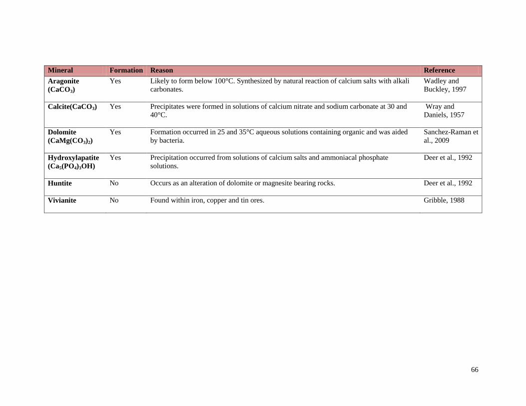
66

Mineral Formation Reason Reference

Aragonite

(CaCO3)

Yes Likely to form below 100°C. Synthesized by natural reaction of calcium salts with alkali

carbonates.

Wadley and

Buckley, 1997

Calcite(CaCO3) Yes Precipitates were formed in solutions of calcium nitrate and sodium carbonate at 30 and

40°C.

Wray and

Daniels, 1957

Dolomite

(CaMg(CO3)2)

Yes Formation occurred in 25 and 35°C aqueous solutions containing organic and was aided

by bacteria.

Sanchez-Raman et

al., 2009

Hydroxylapatite

(Ca5(PO4)3OH)

Yes Precipitation occurred from solutions of calcium salts and ammoniacal phosphate

solutions.

Deer et al., 1992

Huntite No Occurs as an alteration of dolomite or magnesite bearing rocks.

Deer et al., 1992

Vivianite No Found within iron, copper and tin ores.

Gribble, 1988

67

The mass balance part of the model was done using Excel. This accounts for the loss of metals via

the effluent and sludge and for the addition of metals through the feed. The first cycle was modelled

by taking the initial ion concentrations from the WEST model and adding the ions in the feed as

follows:

(

)

( ) ( )

The final concentration of each ion found within the reactor from the equation above then formed

the input concentrations for the VM speciation modelling. After the model was executed, the output

from VM included the total soluble ion concentrations (in the sludge and supernatant) and the total

concentration of ions within precipitates (which is the concentration of ions in the sludge since the

precipitates are associated with the solid phase). This output of concentrations from the speciation

model represents the concentrations in the reactor at the end of the first cycle.

Mass balances to thereafter account for the loss and gain of ions from decanting and feeding for the

next cycle were required. The following equations provide these

(

)

( )

Where:

(

) ( )

(

) ( )

(

) ( )

(

) ( )

( )

68

The final concentration in the reactor found for each ion was then used as an input into the

speciation model and the output represented the ion concentrations at the end of the cycle. This

combination of mass balance equations and speciation modelling was repeated until the ion

concentrations reached a quasi-steady state. For the washout experiment in Experiment B, the same

mass balance equations applied with the exception that no moles of micronutrients were added in

the feed. An illustration of the mass balance for both Experiment A and B is provided in Appendix

D.

69

4. Results

When analysing the experimental data for both Experiment A and B, certain micronutrients were

assessed. These included metals that are known from literature to be required by microorganisms

for their various functions. Certain metals were excluded from the results of Experiment A and B as

they were either not detectable during ICP-AES analysis or an error occurred during the calibration

step. A calibration error occurs when the standard solutions prepared for a metal do not return a

linear calibration graph when analysed. Metals are not detectable by the instrument when they

occur in very low concentrations that are near or below the detection limit. The following table

provides a summary of the metals assessed:

Table 17: Metals Inventory.

Metals : Ca Mg Fe Co Cr Cu Mn Al Zn Ni

Experiment A: ** Mg Fe * Cr Cu * Al Zn Ni

Experiment B: Ca Mg Fe Co Cr Cu Mn Al Zn *

* Not detectable ** Calibration Error

4.1 Experiment A Results Experiment A included a metals mass balance for two cycles, cycle (i) and cycle (ii). These cycles

were analysed in sequence thus the final sludge of cycle (i) was the same as the initial sludge of

cycle (ii). A sequential extraction experiment on the initial and final sludge samples for both cycles

was also performed. The sum of the metals obtained from the sequential extraction was then

compared to the metals obtained from the acid digestion to provide an indication of the

effectiveness of the sequential extraction. These were all performed for both reactor I (Glucose

feed) and reactor II (Ethanol feed).The results obtained for both the reactors are presented in the

following sections.

4.1.1 Metals Mass Balance

A metals mass balance was performed to assess whether all the metal entering and leaving the

system can be accounted for. Metals entering consisted of those within the feed and sludge at the

start of the cycle while metals exiting consisted of those within the decanted supernatant and sludge

at the end of cycle. All these values were obtained from ICP-AES analysis with an acid digestion

preceding the determination of metal concentration in the sludge and decant samples. The following

figure presents the metals mass balance for cycle (i) for metals in the concentration range of 100-

70

2000 mg within the reactor for reactor I and II. The mass balance was calculated according to

equation (2).

Figure 9: Metals mass balance (range 100-2000 mg) for Cycle (i) Reactor I and II.

Looking at the figure above, the contribution of the metals within the feed and decant is small

compared to the amounts presented in the sludge. For Reactor I, their contribution may be regarded

as negligible but for Reactor II, the decant accounts for a sizable amount of the metals at the end of

the cycle. This indicates that the metals have accumulated in a form associated with the sludge

phase for both reactors while for Reactor II, the metals occur in a soluble form as well. A noticeable

feature for Al, Zn, Fe and Mg of Reactor I and Zn and Fe of Reactor II is that the calculated mass of

metals at the end of the cycle is less than the metals at the start of the cycle. Since the majority of

metals reside in the sludge, the discrepancy could be due to the way the mass of sludge, before and

after the cycle, was calculated. The determination of the mass of sludge (section 3.1.4) was

necessarily approximate because the cycles for which the analysis was performed were in a period

of continuous operation of the reactor. Under these conditions, the reactor cannot be opened since

oxygen poisons the microorganisms. Therefore there is significant uncertainty in the mass of sludge

which was determined from the height of the settled sludge and the density of the sludge.

Cu, Cr and Ni were contained within a much smaller range than the metals above. The figure below

provides the mass balance for cycle (i), Reactor I and II for metals with a total mass in the reactor

below 100mg.

0

200

400

600

800

1000

1200

1400

1600

1800

2000

Alstart

RI

AlendRI

AlstartRII

AlendRII

Znstart

RI

ZnendRI

ZnstartRII

ZnendRII

Festart

RI

FeendRI

FestartRII

FeendRII

Mgstart

RI

MgendRI

MgstartRII

MgendRII

Cal

cula

ted

to

tal m

eta

l mas

s in

th

e r

eac

tor

(mg)

Feed Sludge Start Decant Sludge End

71

Figure 10: Metals mass balance (range 0- 100 mg) for Cycle (i) Reactor I and II.

From the figure above, it may be seen that majority of the metals are found within the sludge for

both reactors. For Reactor I, the metals found within the feed and decant are negligible while for

Reactor II, with the exception of Ni, the decant contains a sizeable amount, similar to the

observations for Al, Zn, Fe and Mg. Another similar observation to Al, Zn, Fe and Mg is the

discrepancy between the mass of metals at the start and at the end of a cycle where the mass at the

start is consistently higher than at the end of the cycle.

4.1.2 Sequential Extraction of Sludge

The sequential extraction was performed on the sludge using different reagents sequentially to

extract metals from different phases. This was done for sludge samples from Cycle (i) initial

sludge, Cycle (i) final sludge (i.e. the initial sludge for Cycle (ii)) and Cycle (ii) final sludge. These

are referred to as 1,2 and 3 respectively in the figure that follows.

0

10

20

30

40

50

60

Custart

RI

CuendRI

CustartRII

CuendRII

Crstart

RI

CrendRI

CrstartRII

CrendRII

Nistart

RI

NiendRI

NistartRII

NiendRII

Cal

cula

ted

to

tal m

eta

l mas

s in

th

e

reac

tor

(mg)

Feed Sludge Start Decant Sludge End

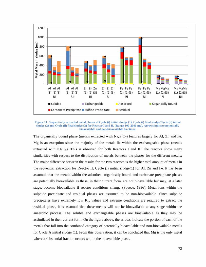
72

Figure 11: Sequentially extracted metal phases of Cycle (i) initial sludge (1), Cycle (i) final sludge/Cycle (ii) initial

sludge (2) and Cycle (ii) final sludge (3) for Reactor I and II. (Range 100-2000 mg). Arrows indicate potentially

bioavailable and non-bioavailable fractions.

The organically bound phase (metals extracted with Na4P2O7) features largely for Al, Zn and Fe.

Mg is an exception since the majority of the metals lie within the exchangeable phase (metals

extracted with KNO3). This is observed for both Reactors I and II. The reactors show many

similarities with respect to the distribution of metals between the phases for the different metals;

The major difference between the results for the two reactors is the higher total amount of metals in

the sequential extraction for Reactor II, Cycle (i) initial sludge(1) for Al, Zn and Fe. It has been

assumed that the metals within the adsorbed, organically bound and carbonate precipitate phases

are potentially bioavailable as these, in their current form, are not bioavailable but may, at a later

stage, become bioavailable if reactor conditions change (Speece, 1996). Metal ions within the

sulphide precipitate and residual phases are assumed to be non-bioavailable. Since sulphide

precipitates have extremely low Ksp values and extreme conditions are required to extract the

residual phase, it is assumed that these metals will not be bioavailable at any stage within the

anaerobic process. The soluble and exchangeable phases are bioavailable as they may be

assimilated in their current form. On the figure above, the arrows indicate the portion of each of the

metals that fall into the combined category of potentially bioavailable and non-bioavailable metals

for Cycle A initial sludge (1). From this observation, it can be concluded that Mg is the only metal

where a substantial fraction occurs within the bioavailable phase.

0

200

400

600

800

1000

1200

Al(1)

Al(2)RI

Al(3)

Al(1)

Al(2)RII

Al(3)

Zn(1)

Zn(2)RI

Zn(3)

Zn(1)

Zn(2)RII

Zn(3)

Fe(1)

Fe(2)RI

Fe(3)

Fe(1)

Fe(2)RII

Fe(3)

Mg(1)

Mg(2)RI

Mg(3)

Mg(1)

Mg(2)RII

Mg(3)

Me

tal M

ass

in s

lud

ge (

mg)

Soluble Exchangeable Adsorbed Organically Bound

Carbonate Precipitate Sulfide Precipitate Residual

73

The figure that follows provides the sequentially extracted metals for Cu, Cr and Ni (range 0-100

mg) for reactor I and II.

Figure 12: Sequentially extracted metal phases of Cycle A initial sludge (1), Cycle A final sludge/Cycle B initial

sludge (2) and Cycle B final sludge (3) for reactor I and II. (Range 0-100 mg).

The data observed above seems dubious as there is no consistency between the cycles and Ni,

which was found in the mass balance in figures 11 and 12 above, for reactors I and II respectively,

is now non-existent for both reactors. For the samples in question, the concentration of the metal

ion in each sample for the ICP-AES analysis was close to the calibration limit and therefore the

magnitude of error in each measurement was high. When calibration was performed, the lowest

concentration calibrated for was 0.01 mg/l (equivalent to an end result of approximately 4 mg of

metal in the sludge). This is relatively close to reported detection limits of 0.005 mg/l for Cu, 0.006

for Cr and 0.015 mg/l Ni (Martin et al., 1998). The results therefore suggest that the uncertainty in

these measurements renders the results meaningless, and nothing can be inferred about the

distribution of these metals between phases except (with caution) that a significant portion of

chromium ions are present in an organically bound form.

4.1.3 Comparison between Acid Digestion and Sequential Extraction

Acid digestion was used to determine the total amount of metals within the sludge samples.

Sequential extraction was used to determine the distribution of metals between the different

extractable phases within the samples. The sum of these phases should theoretically be equal to the

total amount of metals. The figures below show these comparisons for Al, Zn, Fe and Mg for Cycle

0

5

10

15

20

25

Cu(1)

Cu(2)RI

Cu(3)

Cu(1)

Cu(2)RII

Cu(3)

Cr(1)

Cr(2)RI

Cr(3)

Cr(1)

Cr(2)RII

Cr(3)

Ni(1)

Ni(2)RI

Ni(3)

Ni(1)

Ni(2)RII

Ni(3)

Me

tal M

ass

in s

lud

ge (

mg)

Soluble Exchangeable Adsorbed Organically Bound

Carbonate Precipitate Sulfide Precipitate Residual

74

A initial sludge (1), Cycle A final sludge/Cycle B initial sludge (2) and Cycle B final sludge (3) for

reactor I and II.

Figure 13: Comparison of metals determined using acid digestion and sequential extraction for Al, Zn, Fe and Mg

for reactor I and II with standard deviations.

The greatest discrepancies between the metals determined using acid digestion and the sum of the

sequentially extracted metals for both reactors occurs for measurements of Fe. For Fe, the metal

with the highest total concentration, the difference between the two values is in the range of 30-

55% with the metals extracted using acid digestion being consistently higher than the sum of

sequentially extracted metals.

The graph above also shows the standard deviations (from replicate samples) calculated for the acid

digestion and the sequential extraction analysis. From the graph it is clear that there is a

significantly larger amount of error involved with sequential extraction analysis when compared to

the acid digestion analysis. This is because the sequential extraction measurements comprise of

measurements obtained from each of the extracted phases and there is a standard deviation

associated with each phase. The net result which is based on the sum of the seven different phases

will inherently include the associated uncertainty from each phase.

4.1.4 Mass Balance-Speciation Modelling Results- Experiment A

A combination of Visual Minteq (VM) and Microsoft Excel was used for the mass balance-

speciation modelling. For each cycle, the effect of decanting and feeding, as well as growth were

0

200

400

600

800

1000

1200

1400

1600

1800

2000

Al(1)

Al(2)RI

Al(3)

Al(1)

Al(2)RII

Al(3)

Zn(1)

Zn(2)RI

Zn(3)

Zn(1)

Zn(2)RII

Zn(3)

Fe(1)

Fe(2)RI

Fe(3)

Fe(1)

Fe(2)RII

Fe(3)

Mg(1)

Mg(2)RI

Mg(3)

Mg(1)

Mg(2)RII

Mg(3)

Me

tal M

ass

(mg)

Acid Digestion Sequential Extraction

75

accounted for using mass balances in Excel. VM was used to determine the chemical speciation of

the system at the end of each cycle just before decanting. Results from VM were used as an input to

the mass balances in Excel and once decanting, feeding and growth were accounted for, resultant

values were used as an input to VM. This process was performed until the system reached steady-

state with respect to ion concentrations.

Since the initial conditions as well as the assumptions made for reactor I and II were similar (with

the exception of gas partial pressures), the results obtained were similar. For the sake of avoiding

repetition, only results obtained for reactor I will be discussed, however, results for reactor II are

presented in Appendix E. The number of cycles modelled does not represent experimental cycles,

but is the number required until the soluble ion concentrations at the end of each modelled cycle are

approximately constant.

4.1.4.1 Soluble Concentration Changes

At this stage, only modelling of the precipitation phase has been performed to see whether the

precipitation is controlling and if just modelling this phase is sufficient to describe the data. Since

only precipitation is considered, for an ion that does not precipitate, the concentration of the

supernatant will tend towards the concentration at which the ion is being added before each cycle.

If the initial supernatant concentration is higher than the concentration at which the ion is added,

the supernatant will get diluted each cycle when decanting and adding the feed is performed until

the ion reaches the concentration it has in the feed. Similarly, for an ion where the initial

supernatant concentration is lower than in the feed, the supernatant concentration will increase with

each cycle, tending towards the concentration it has in the feed.

Figure 14 shows the model prediction of concentration of ions in the dissolved phase for those ions

in the mg/l range and how they change with each successive cycle modelled. The graph also

displays the comparison between the model predicted value (over 20 hypothetical cycles from the

assumed initial condition) and the soluble concentration determined experimentally for the

magnesium and iron ions. The experimental values correspond to the supernatant soluble metal

concentration associated with the cycle A initial sludge, cycle A final sludge/cycle B initial sludge

and the cycle B final sludge.

76

Figure 14: Concentration of ions in the dissolved phase for Ca, Fe, K and Mg ions, and their changes with each

successive cycle modelled for Reactor I, including comparisons to experimental values for Fe and Mg (mg/l).

The model predicted graphs represent a number of points where each point represents one cycle

modelled. At a glance, the system reaches a pseudo-steady state whereby the species reach a

constant concentration. For all the ions the concentrations are predicted to increase from the initial

point until they plateau. This is due to the selected hypothetical initial concentrations being lower

when compared to the concentration that the species tend to. As a function of the model

assumptions, the species concentrations should tend to the concentration that is added via the feed

for each cycle if that species is not being precipitated. This is observed for the potassium,

magnesium and calcium ions where the model feed concentrations were 3.41, 1.08 and 0.34 mg/l

respectively, matching the final predicted supernatant concentrations. For iron, the feed

concentration was 0.52 mg/l but when compared to the final modelled dissolved concentration 0.25

mg/l, it would indicate that the model predicts that this metal is being precipitated.

With regards to the comparison between the predicted and experimentally determined values, the

experimentally determined values for both iron and magnesium are higher than the model

predictions. The largest discrepancy exists with magnesium where the experimental values are

approximately three times higher than the model predicted values. Since the experimentally

0.0

0.5

1.0

1.5

2.0

2.5

3.0

3.5

4.0

0 5 10 15 20 25

Solu

ble

ion

co

nce

ntr

atio

n (

mg/

l)

Cycle

Fe2+ Exp Mg2+ Exp Ca2+ Fe2+ K+ Mg2+

77

determined values are higher, it suggests the possibility that there are other processes or mass

transfer effects that may be involved.

Figure 15 displays the predicted dissolved ion concentrations for species in the µg/l range, and their

changes with modelling each successive cycle. The graph also displays the comparison between the

predicted value and the concentration determined experimentally for copper and zinc.

Figure 15: Concentration of ions in the dissolved phase for Mn, Cu and Zn ions (µg/l), and their changes with each

successive cycle modelled for Reactor I, including comparisons to experimental values for Cu and Zn.

While most ions have reached a level dissolved concentration, the manganese ion displays a trend

that is increasing continually at an increasing rate. This trend suggests that manganese, which has a

feed concentration of 28 µg/l, was initially predicted to precipitate but then started to dissolve into

the soluble phase in the latter cycles, causing the predicted soluble concentration to increase. If no

further precipitation is predicted as more cycles are modelled, the soluble concentration would

increase and tend towards the feed concentration of 28 µg/l. This is further elaborated on in the

following section on precipitate formation (section 4.1.4.2).

0.0

1.0

2.0

3.0

4.0

5.0

6.0

7.0

8.0

0 5 10 15 20 25

Co

nce

ntr

atio

n (μ

g/l)

Cycle

Mn2+ Cu2+ Exp Zn2+ Exp Cu2+ Zn2+

78

The feed concentration for both copper and zinc was 5 µg/l. Since the final model predicted values

were significantly lower for both copper (0 µg/l) and zinc (0.73 µg/l) the model suggests that all of

the copper ions and most of the zinc ions will be sequestered in precipitates. This is somewhat

reflected in the experimental analysis where both zinc and copper were not found in the soluble

phase (figures 11 and 12 respectively). Although the model predicts that some zinc will occur in the

soluble phase, the discrepancy between the model predicted and experimentally determined values

could be attributed to the difficulty and limitations associated with determining metal

concentrations in the micro ranges experimentally.

The graph that follows displays the dissolved ion concentrations for ionic species Co2+

and HS-1

, in

the μg/l range, as well as their changes with modelling each successive cycle.

Figure 16: Concentration of ions in the dissolved phase for Co2+ and HS-1 (μg/l), and their changes with each

successive cycle modelled for Reactor I.

The two ions above are predicted to occur in minute concentrations. The model predicts that these

ions reach concentrations of about 0.08 and 0.15 μg/l for the cobalt and hydrogen sulphide ions

respectively. Although sulphur is regarded as a macronutrient, since it is required by

microorganisms and dosed into the system in macro concentrations, it is found in the soluble micro

concentration range (µg/l range). Since the metals would precipitate with S2-

ion and the amount of

S2-

ion is dictated by the HS- ion (depending on the pH), this suggests that bulk of the S

2- lies in one

of the other metal phases. For cobalt, the feed concentration was 37 µg/l, and it was not detected

experimentally, possibly because the concentration in the soluble phase was below the detection

0.00

0.05

0.10

0.15

0.20

0.25

0.30

0 5 10 15 20 25

Co

nce

ntr

atio

n (μ

g/l)

Cycle

Co2+ HS-1

79

limit. This suggests that, like the bi-sulphide ion (S2-

), a significant portion of this ion is predicted

to occur in phases other than the soluble phase.

4.1.4.2 Precipitate Formation

VM and the mass balance-speciation model predicts the formation of a number of possible

precipitates. From this list, precipitates most likely to occur under reactor conditions were allowed

to precipitate. A key result from this was the percentage of a metal ion that was found within

precipitates. The following graph displays the changes in the amount of ion within precipitates with

each cycle modelled. To compare this percentage to the experimental data, it would be necessary to

separate the experimental data into either the soluble or precipitate phase since the model only

predicts the soluble and precipitate phases. Therefore, for this comparison, the ions from the

supernatant analysis are regarded as soluble ions and the ions from the total acid digestion minus

the ions from the supernatant analysis are regarded as within precipitates.

Figure 17: Percentage of ions that are within precipitates as predicted for each successive cycle modelled together

with the values obtained from experimental data for Mg, Ca, Fe, Cu and Zn.

0

20

40

60

80

100

120

0 5 10 15 20

% o

f io

n w

ith

in p

reci

pit

ate

s

Cycle

Ca2+ Co2+ Cu2+ Fe2+ HS-1K+ Mg2+ Mn2+ Zn2+ Mg2+ ExpFe2+ Exp Zn2+ Exp Cu2+ Exp

Cu2+

, Zn2+

, Fe2+

Exp

Mg2+

Exp

HS-1

, Cu2+

, Co2+

Zn2+

Mg2+

, K+

, Ca2+

Mn2+

Fe2+

80

A significant result from the graph above is that the model predicts that certain metals occur

completely within precipitates from the start of the experiment. These metals include Co2+

, Cu2+

and also the anion HS- (not measured experimentally). This suggests the possibility that these

metals may never occur in a bioavailable phase for micronutrient absorption. Mn2+

is initially

predicted to occur mostly within precipitates, however, as conditions change with each cycle

modelled, the amount found within precipitates decreases. This was reflected in Figure 15 where an

increase in the Mn2+

soluble concentration was observed through the cycles. A similar trend for

Zn2+

and Fe2+

are observed where the amount of ion predicted to occur within precipitates are

initially higher and then decrease through the cycles as conditions within the reactor change. For

Mg2+

, K+ and Ca

2+, the model predicts that these metals occur within the soluble phase only.

Since the experimental values representing precipitates are taken as the total ions from the acid

digestion minus the soluble ions from the supernatant analysis, it is anticipated that the amount of

precipitates will be over-represented. When comparing the predicted values to the experimentally

determined values, a large discrepancy exists and part of this is due to the over-representation of

precipitates for the experimental values. With the exception of Cu2+

which compares well to the

model predicted value, the experimental values for the rest of the ions are higher than the model

predicted values.

4.2 Experiment B Results While a detailed discussion on the significance of the results from Experiment A is presented in

section 5.1, the following broad observations were made:

Due to the number of experimental steps involved in the sequential extraction procedure,

multiple and compounding errors are expected.

The small quantities of metals expected in the different phases for micronutrients are close

to the calibration limit, resulting in high magnitude of uncertainty in the reported values.

It is more essential to know the bioavailable metals from the potentially bioavailable and

non-bioavailable metals than to know the actual distribution of the metals between the

phases as defined by the sequential extraction procedure.

An operational decision on whether to get detailed bioprocess data (pH, gas flow and composition)

or detailed metals data (sequential extraction) had to be made as time did not permit obtaining both.

Sequential metal extraction was omitted since the results from Experiment A indicated that with the

current methodology and equipment, the uncertainty in the sequential extraction measurement was

large. In addition, the model currently only considers a solid and soluble phase for metal speciation;

81

therefore, although the sequential extraction experiment would provide additional information on

the metal speciation, it was decided that the detailed bioprocess data would be of more value at this

stage in the research.

The bioprocess response data was supported by soluble and total metals data since that was the

level required for the model. Therefore, this set of experiments also tests whether modelling only

soluble and precipitated metals adequately describe metal dynamics. The analysis of the metals

within the supernatant was used to provide the soluble, bioavailable fraction while the sludge metal

analysis was used to provide the potentially bioavailable and non-bioavailable fractions. This was

deemed a sufficient estimation as for most metals (excluding Mg) the sequential extraction

experimental data indicated that the sludge contained a negligible amount of metals in the soluble

and exchangeable phases. Sludge and supernatant samples were thus collected and analyzed for

metals using ICP-AES for supernatant samples and acid digestion with ICP-AES for the sludge

samples. This was done for selected samples only.

FTRW was used as the sole basic food for Experiment B. Experiment B consisted of running

reactors from start-up for a few months and thereafter performing a micronutrient washout

experiment. Negative cycle numbers represent cycles during the start-up phase and cycle 0

represents the first cycle with no micronutrients added to the feed. So while Experiment A only

contained data for pseudo-steady state operation, the Experiment B data set presents results for a

series of cycles for which the end of cycle metal concentration is expected to change with each

cycle.

Experiment B was performed on two reactors, Reactor I and II. The conditions were identical in

both reactors and thus provided validation of results. The results obtained for both reactors were

similar with respect to the trends observed in the data as well as the actual numbers obtained.

Therefore, only results obtained for reactor II will be presented in this section however, in some

cases, where anomalies were observed and both results require comparison, results for both reactors

are presented. A full set of results for reactor I may be found in Appendix F.

The results for reactor II were used for comparisons between the experimental data and the model

predicted data. For the sake of continuation, the results from the model are presented first. The

model has the same conceptual approach as in Experiment A but in this case, the washout of metals

was also being modelled by calculating the new supernatant metal concentration at the end of each

cycle and removing a portion with the decant.

82

4.2.1 Mass Balance-Speciation Modelling Results- Experiment B

The mass balance-speciation modelling was carried out using the assumptions mentioned in the

methodology section (section 3.3.3). Since both reactors have the same initial conditions and feed,

the model is representative of both. From the initial conditions, the successive feed-react-decant

cycles were modelled until the dissolved and precipitate concentrations reached a pseudo-steady

state. Thereafter, the metals washout experiment was modelled. Cycles below zero represent cycles

modelled with a micronutrient cocktail in the feed. Cycle 0 and above represent those cycles

modelled where no micronutrients were dosed to the system.

4.2.1.1 Precipitate formation

The following graph shows the types of precipitates predicted, their concentrations as well as their

reduction due to micro-metal washout.

Figure 18: Model prediction of the concentrations of different precipitates formed and their changes with each

cycle modelled.

The main feature of the graph above is that from the moment the metal washout is modelled (Cycle

-1 to 0), the concentrations of the precipitates are predicted to decrease. By Cycle 2, the

concentrations of the precipitates have reduced to micro-quantities in the nano and pico g/l ranges.

1.00E-09

1.00E-08

1.00E-07

1.00E-06

1.00E-05

1.00E-04

1.00E-03

1.00E-02

1.00E-01

1.00E+00

1.00E+01

-4 -3 -2 -1 0 1 2 3 4 5 6

Co

nce

ntr

atio

n (

mg/

l)

Cycle Covellite (CuS) NiS

CoS Sphalerite (ZnS)

MoS2 Pyrite (FeS2)

MnHPO4 Hydroxyapatite (Ca5(PO4)3OH)

83

The graph that follows displays the percentage of the total ions predicted to be within these

precipitates, as well as the rate at which these are released from the precipitates due to the metal

washout.

Figure 19: Percentages of the metal ions found within precipitates and their changes with each cycle modelled.

With the exception of calcium, hydrogen sulphide and magnesium, the metal ions are predicted to

occur only within precipitates prior to the metal wash-out. This suggests that these ions, like

copper, cobalt and hydrogen sulphide from experiment A (refer to figure 17, section 4.1.4.2) are

locked within precipitates and are not in a bioavailable phase for micronutrient absorption.

It is apparent from the graph above that the metal ions found within the precipitates wash out at

different stages. The first metal that is not present in precipitates is calcium which is depleted in

cycle 0. Manganese is predicted to be released from precipitates by cycle 3 while zinc and cobalt

are released by cycle 7 followed by nickel released by cycle 9. Iron, copper and molybdenum are

released by cycles 11, 18 and 20 respectively.

0

20

40

60

80

100

120

-5 0 5 10 15 20

% o

f Io

n in

Pre

cip

itat

es

Cycle

Ca2+ Co+2 Cu+2 Fe+2 HS-1

Mg2+ Mn2+ MoO4 2- Ni2+ Zn2+

84


The changes in soluble ion concentrations for the model based on Experiment B will be presented

in this section. These concentrations are also compared to the experimental values wherever these

have been determined. Mg, Ca, and Fe were detectable during the experimental analysis and are

included in the analysis that follows. However, Co, Cu, Mn, Zn and Ni were not detected.

The graph that follows displays the soluble concentrations for Mg and Ca determined from the

speciation modelling together with the values determined experimentally from the supernatant ICP-

AES analysis.

Figure 20: Concentration of ions in the dissolved phase for Mg and Ca, and their changes with each successive

cycle modelled for Reactor II, including comparisons to experimental values.

From the start of the washout experiment, both Mg and Ca experience a decrease in the soluble

concentrations. The experimental values for Mg are comparable with those determined from the

model; however for Ca this is not the case. The predicted Ca concentrations are in the range of 0.82

to 0.05 mg/l while the experimental values range from 16 to 4.5 mg/l.

A similar graph was plotted for the concentrations for Mn and Zn with the exception that these

metal ions were not experimentally detected in the supernatant. The following graph shows the

predicted dissolved concentration values and their changes with the washout experiment.

0

2

4

6

8

10

12

14

16

18

-5 0 5 10 15 20 25

Dis

solv

ed

Co

nce

ntr

atio

n (

mg/

l)

Cycle

Ca2+ Mg2+ Mg Exp Ca Exp

85

Figure 21: Concentration of ions in the dissolved phase for Mn (in mg/l x10-4) and Zn (in mg/l x10-8) and their

changes with each successive cycle modelled for Reactor II.

The model predicts that these two ions occur in minute quatities with Mn in the approximate micro

range and Zn in the approximate pico range. Nevertheless, the effect of a metal washout experiment

may be observed, although the magnitude of the model predictions suggests that these values will

not be measured accurately using any available techniques. The Mn soluble concentration initally

increases with the washout experiment and thereafter from cycle 3 decreases. For Zn, the

concentration starts decreasing from cycle 7 onwards.

The graph that follows displays the chages in soluble concentration as predicted by the mass

balance-Speciation model for Co, Fe and Ni.

0.0

1.0

2.0

3.0

4.0

5.0

6.0

-5 0 5 10 15 20 25

Dis

solv

ed

Co

nce

ntr

atio

n

Mn

: mg/

l x1

0-4

Zn

: mg/

l x1

0-8

Cycle

Mn2+ Zn2+

86

Figure 22: Concentration of ions in the dissolved phase for Co, Fe and Ni as predicted by the model.

The predicted dissolved concentrations for Co, Fe and Ni are in minute quantities suggesting that

the bulk of these ions are locked up within precipitates. Once the metal washout experiment was

performed, Co was predicted to have started decreasing by cycle 7 and Ni by cycle 9. For Fe, a

small decrease is observed from the washout until cycle 10. Thereafter, the concentration of Fe is

reduced at the same rate as that of Ni. The graph that follows displays the model predicted

concentration of Fe in the dissolved phase as compared to the experimentally determined values.

0.0E+00

5.0E-10

1.0E-09

1.5E-09

2.0E-09

2.5E-09

-5 0 5 10 15 20 25

Dis

solv

ed

Co

nce

ntr

atio

n (

mg/

l)

Cycle Co+2 Fe+2 Ni2+

87

Figure 23: Concentration of Fe ions in the dissolved phase as predicted by the model compared to the

experimentally determined values

Although the experimental values determined for Fe follow a similar trend to those of the predicted

concentrations (as seen in figure 31 above), the numbers are extremely different as the graph above

suggests. This indicates that either there is experimental uncertainty for the measured values or that

the precipitates are not in equilibrium, either due to mass transfer or redox effects.

Cu and Mo (shown as molybdate ion) were predicted to occur in x10-18

mg/l and x10-22

mg/l

quantities respectively. The graph below shows the washout for these two ions, with Cu values in

mg/l x10-18

and Mo values in mg/l x10-22

.

0.00

0.20

0.40

0.60

0.80

1.00

1.20

1.40

-5 0 5 10 15 20 25

Dis

solv

ed

Co

nce

ntr

atio

n (

mg/

l)

Cycle Fe Exp Fe+2

88

Figure 24: Washout pattern observed for the soluble concentrations of Cu and Mo (as MoO42-) as predicted by the

model

Besides the observation that these ions occur in extreme micro quantities, the graph above shows

that these ions soluble concentrations reduce from the start of the washout experiment. However,

this rate increases by cycle 18 for Cu and by cycle 21 for Mo due to the predicted depletion of the

precipitates.

4.2.2 Supernatant Metal Analysis

For Experiment B, metal analysis was conducted only using ICP-AES and acid digestion where

required. Sequential metal extraction was omitted since the results from Experiment A indicated

that with the current methodology and equipment, the uncertainty in the sequential extraction

measurement was large and since the model currently only considers a solid and soluble phase for

metal speciation.

The supernatant extracted from the reactors contained minimal solids and after filtration, the

samples were subjected to ICP-AES. The concentrations found represent soluble concentrations. In

order to make a comparison between cycles and between different metals, concentrations in the

following analysis are presented as supernatant concentration as a % of the maximum supernatant

concentration. The challenge with plotting the different metal concentrations on the same axis is

that their concentrations are order of magnitudes different, and the feed concentrations likewise. In

order to observe what is happening with all the metals, it is necessary to normalise and present the

data on a relative basis. Furthermore, the objective is to see whether there is any evidence of metal

washout in the soluble or solid phases, thus the data have been presented this way. The following

0.00

0.50

1.00

1.50

2.00

2.50

3.00

-5 0 5 10 15 20 25

Dis

solv

ed

Co

nce

ntr

atio

n

Cu

: m

g/l x

10

-18

M

o: m

g/l x

10

-22

Cu+2 MoO4 2-

89

graph displays the soluble concentrations of Al, Ca, Mg and Fe as a percentage of their maximum

concentration as well as the amount of the metal washout in the effluent as a percentage of the

amount of metal in the feed when dosed to the system (% metal loss). Co, Cr, Cu, Mn and Zn were

not detectable within the supernatant and therefore are not included. Al is not a micronutrient dosed

to the system, thus there is not a % metal lost as a function of metal in the feed.

Figure 25: Measured soluble concentrations as a percentage of the maximum concentration measured as well as

the amount of metal lost as a % of the feed for selected cycles only.

Excluding Al, the overall trend for the soluble metal concentrations is a decreasing one. There is a

minimal difference in concentration between cycles -3 and -2, which are cycles before the washout

experiment. For cycle 9, which is the 10th cycle for which metals were not dosed as micronutrient,

the concentrations for Ca and Mg have decreased significantly from values obtained before

washout was initiated. The concentrations continue to drop until cycle 15. For Fe, there is also a

decreasing trend however it is more subtle than those observed for Ca and Mg. Only in cycle 15 (16

cycles after the washout), the concentration decreases to about 25% of the maximum value.

Although from cycle -3 to cycle 15 the Al concentration decreases to about 30% of the value from

cycle -3, a definitive decreasing trend is not observed.

The % metal lost in the supernatant for Ca is five times greater than the amount fed before the

metal washout experiment. For cycles 9, 10, 14 and 15, Ca is still lost at a rate of between 1.6 and

2.5 times the feed mass even though during these cycles, no Ca is fed to the system. This indicates

that accumulated Ca is being rapidly depleted by dissolution of precipitates or release from some

0%

20%

40%

60%

80%

100%

120%

-3 -2 9 10 14 15

% C

/Cm

ax

Cycle Al (C/Cmax) Ca (C/Cmax) Fe (C/Cmax) Mg (C/Cmax)

→ % metal loss

46 43

31 27

94

108

223 252 188

161

485 543 11

11 11

12

9

3

90

other solid phase that has sequestered Ca. For Fe, only 11-12 % of what was being fed was lost via

the effluent. For cycles where no Fe was dosed, the % metal lost is still similar, except for cycle 15

where only 3% is lost. This suggests that the Fe is possibly depleted within the reactor. For Mg, the

near 100% metal lost for cycles -3 and -2 suggest that the same amount dosed to the system is the

same amount lost via the effluent. This indicates that there is no net accumulation or depletion of

Mg during a cycle with micronutrient dosing. For cycles during the washout experiment, Mg is still

lost but at a decreasing rate.

4.2.3 Sludge Metal Analysis

Selected sludge samples were collected and subjected to acid digestion before undergoing ICP-AES

analysis. The sludge metal concentrations represent phases which are potentially or non-

bioavailable such as precipitates. The graph that follows displays the sludge metal concentrations as

a percentage of the maximum concentration (% C/Cmax) for Al, Ca, Co, Cr, Cu, Fe, Mg, Mn and

Zn.

Figure 26: Sludge metal concentrations as a function of the maximum concentration measured for selected cycles

for Al, Ca, Co, Cr, Cu, Fe, Mg, Mn and Zn.

If one discounts the last cycle, a fluctuating trend for most metals are observed. This is clearly

shown when observing that not all the metals have a maximum measured concentration at cycle -3.

For Al, Cu, Fe and Zn, the maximum concentration of metal within the sludge is found in cycle 10.

0%

20%

40%

60%

80%

100%

120%

-3 -2 9 10 14 15

% C

/Cm

ax

Cycle

Al Ca Co Cr Cu Fe Mg Mn Zn

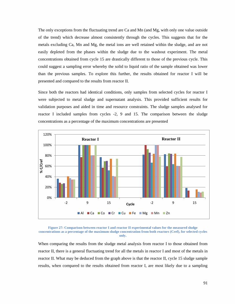
91

The only exceptions from the fluctuating trend are Ca and Mn (and Mg, with only one value outside

of the trend) which decrease almost consistently through the cycles. This suggests that for the

metals excluding Ca, Mn and Mg, the metal ions are well retained within the sludge, and are not

easily depleted from the phases within the sludge due to the washout experiment. The metal

concentrations obtained from cycle 15 are drastically different to those of the previous cycle. This

could suggest a sampling error whereby the solid to liquid ratio of the sample obtained was lower

than the previous samples. To explore this further, the results obtained for reactor I will be

presented and compared to the results from reactor II.

Since both the reactors had identical conditions, only samples from selected cycles for reactor I

were subjected to metal sludge and supernatant analysis. This provided sufficient results for

validation purposes and aided in time and resource constraints. The sludge samples analysed for

reactor I included samples from cycles -2, 9 and 15. The comparison between the sludge

concentrations as a percentage of the maximum concentrations are presented

Figure 27: Comparison between reactor I and reactor II experimental values for the measured sludge

concentrations as a percentage of the maximum sludge concentration from both reactors (Cref), for selected cycles

only.

When comparing the results from the sludge metal analysis from reactor I to those obtained from

reactor II, there is a general fluctuating trend for all the metals in reactor I and most of the metals in

reactor II. What may be deduced from the graph above is that the reactor II, cycle 15 sludge sample

results, when compared to the results obtained from reactor I, are most likely due to a sampling

0%

20%

40%

60%

80%

100%

120%

-2 9 15 -2 9 15

% C

/Cre

f

Cycle


Reactor I Reactor II

92

error. The relative concentrations obtained from cycle15 (reactor II) are significantly lower than the

rest of the samples and does not suggest complete washout of certain metals.

For the sludge samples, when comparing the amount of metal within the sludge to the amount that

was dosed in the feed, the percentage of metal retained (mass of metal in sludge/mass of metal

added in the feed per cycle %) is obtained. The following graph provides the percentage of metal

retained for selected cycles for Ca, Co, Cu, Fe, Mg, Mn and Zn. Al and Cr are not included as they

are not part of the micronutrient cocktail dosed to the system pre-metal washout.

Figure 28: Amount of metal retained within Reactor II as a percentage of the amount dosed via the feed for

selected cycle for Ca, Co, Cu, Fe, Mg , Mn and Zn.

The % metal retained for the different metals range from over 1190% for Zn in cycle -3 to 1.3% for

Mg for cycle 15. For this reason, these values were plotted on a logarithmic scale. Zn and Co

display values of between 700 to 1190% metals retained from cycle -3 to 14, showing great metal

retention. A change is observed for cycle 15, for all the metals, where the % metals retained

decreases. This may be attributed to the lower concentrations measured experimentally, which is

most likely due to a sampling error. Mn, Cu and Fe also show high metal retention. Mg and Ca do

not share this trait as for Mg before the metal washout, only 11% of the metal was found within the

sludge while for Ca, from cycle -3 to 14, metal retention drops from over 100% to just below 50%.

As with the previous figure on metal concentrations as a function of the maximum concentration,

1

10

100

1000

10000

-4 -2 0 2 4 6 8 10 12 14 16

% M

eta

l Re

tain

ed

Cycle

Ca Co Cu Fe Mg Mn Zn

93

cycle 15 shows drastically smaller values, with Co and Cu reaching 0%, even when compared to

just one cycle earlier which was attributed to a sampling error.

4.2.4 Bioprocess Results Calculation and Summary

The bioprocess variables that were monitored during the cycles included biogas production and

composition. The total biogas production for each cycle was calculated using gas flowrates

recorded every half of a second using a gasflow meter. Biogas samples were obtained and analysed

periodically for the first few hours and in the last hour of the cycle using a GC to obtain

instantaneous biogas compositions. Data for cycle 2 and cycle 4 were incomplete due to

uncontrollable power failures in the lab. Therefore, these results have been omitted.

A MATLAB program was developed in-house and used to determine the composition curves of

nitrogen, methane and carbon dioxide for the cycle time. The program predicted the change in

concentration of nitrogen, methane and carbon dioxide by simulating the headspace of the reactor

into which the biogas was released. The average composition of the produced biogas (as opposed to

the concentration accumulated in the headspace) was estimated at several points in time by fitting

the model to the compositions obtained from the GC analysis. The reactor overhead volume was

used as the initial volume for nitrogen. The rate of washout of nitrogen was then estimated from the

overall biogas flow rate and thereafter, the model fitted the predicted compositions for carbon

dioxide and methane to their respective compositions obtained from sampling by adjusting the

produced gas composition. The compositions, together with the cumulative gas production data was

used to produce a cumulative methane production curve with time. This model did not attempt to

describe the biological processes in the ASBR. The graphs that follow show the cumulative gas

production curve, the gas composition changes with time as well as the cumulative methane

production curve as produced from the MATLAB program for cycle -3, Reactor II.

94

Figure 29: The MATLAB graph output for Cycle -3 showing from left to right, cumulative gas production, gas

composition evolution and cumulative methane production with time.

The graphs shown above were generated for all cycles. The maximum methane production rate was

determined from the maximum slope of the cumulative methane production curve. Other variables

such as the maximum estimated CO2 and CH4 compositions were monitored. For pH control, the

minimum pH and to a greater extent, the time taken to recover to a pH of 7 was observed. The table

below summarises the results obtained for all of the cycles under investigation:

95

Table 18: Summary of experimental results for cycles -3 to 15 for Reactor II.

Cycle

Total Biogas

Produced (l)

%

Methane

Recovery

Max

estimated

methane

Composition

Max estimated

CO2

composition

Max Methane

production rate

(gCOD/min) Minimum pH

Time for

recovery to pH

7 (hours)

Alkalinity

dosed (g

NaHCO3)

-3 9.467 100 0.716 0.596 0.133 7.54 0.000 5

-2 10.73 117 0.740 0.595 0.135 7.29 0.000 5

-1 9.787 104 0.720 0.742 0.119 6.73 1.592 5

0 10.31 108 0.709 0.787 0.129 6.8 2.358 5

1 9.541 102 0.731 0.757 0.113 6.84 0.767 5

2*

0.114

5

3 8.221 84.7 0.701 0.683 0.040 6.84 3.033 5

4*

0.101

5

5 6.736 68.4 0.691 0.645 0.074 7.23 0.000 5

6 9.178 102 0.755 0.704 0.117 6.84 5.017 5

7 7.758 82.8 0.723 0.698 0.071 7.4 0.000 5.5

8 9.755 103 0.720 0.649 0.116 6.82 5.200 5.5

9 9.565 107 0.764 0.578 0.120 6.93 0.867 6

10 8.939 100 0.720 0.585 0.122 6.89 1.892 6

11 7.618 78.5 0.700 0.614 0.103 6.79 6.117 6

12 5.426 56.3 0.709 0.525 0.067 6.95 1.075 6.5

13 6.343 68.1 0.730 0.519 0.076 7.02 0.000 6.5

14 5.288 57.6 0.740 0.453 0.055 7.09 0.000 6.5

15 5.833 62.7 0.732 0.497 0.076 7.04 0.000 6.5

* Missing data due to power failure

96

4.2.5 Biogas production, methane activity and methane recovery

The following graph presents the total biogas production, maximum methane activity and the %

methane recovery for cycles -3 to 15 for Reactor II. The % methane recovery was calculated by

finding the total methane production in g COD as a fraction of the feed COD.

Figure 30: The Total biogas production and % methane recovery on the left axis and maximum methane activity

for pre-metal washout cycles -3 to -1 and post-metal washout cycles 0 to 15 on the right axis.

The graph is divided into four regions using purple vertical lines. These have been added to aid the

data interpretation for the graph. For cycles 2 and 4 where the power failure occurred, the

maximum methane production rate was still calculated as the power failure occurred at a time after

the maximum had occurred. For the sake of comparison only, the total biogas produced was

multiplied by 10. Although the three variables correlate well, there is no definitive general trend

observed from the figure above. However, if the graph is observed in the four regions as shown by

the purple lines, the variables initially are unchanging until cycle 2 which corresponds to three

cycles with no micro-metals added. From cycle 2 to cycle 5, a decreasing trend is observed. The

third region, from cycle 5 to cycle 10, seems to be a recovery period where after an initial dip, the

variables increase and stabilize. From cycle 10 onwards the variables are about one third lower than

the values observed before the micronutrient washout.

0.000

0.020

0.040

0.060

0.080

0.100

0.120

0.140

0.160

0

20

40

60

80

100

120

140

-5 0 5 10 15 20

Max

imu

m M

eth

ane

Act

ivit

y (g

CO

D/m

in)

Tota

l Bio

gas

Pro

du

ctio

n (

litre

)

and

% M

eth

ane

Re

cove

ry

Cycle

Total Biogas Produced (*10¯ˡ litres) % Methane Recovery Max CH4 production rate (gCOD/min )

No metals from here

97

4.2.6 pH Control

For the cycle’s pre-metal washout, a dosage of 5 g NaHCO3 was administered. It was anticipated

that during the washout experiment, the micronutrient limitation would affect the microbial activity

in a number of ways including reducing or stopping the rate of biological processes. With the type

and quality of the data, it is not possible to know what particular effects take place however,

general effects can be anticipated. These include changes in gas composition as a result of changes

in CO2 and CH4 producing processes as well as changes in the ability of the microbial population as

a whole to buffer against pH changes.

For each cycle, when the feed was added, there was always an observed reduction in the reactor pH

as a result of the increase in organic acids provided by the feed. However with time, the pH would

rise as the organic acids were converted. By monitoring the time taken for the reactor pH to

stabilise above a pH of 7, an indication of the acid converting activity of the microbes was

provided. As the cycles progressed, a higher dosage of alkalinity was required to allow the pH to

return to a value above 7. If the time taken for a reactor to reach a pH of 7 after the feeding stage

was greater than four hours, then the dosage for the next cycle was increased by 0.5 g NaHCO3.

The graph that follows shows the time taken for the reactor to recover the pH and the amount of

alkalinity dosed for each cycle.

Figure 31: Time required to reach pH recovery and the subsequent increment in dosage for the following cycle for

Reactor II.

0

1

2

3

4

5

6

7

-4 -2 0 2 4 6 8 10 12 14 16

Tim

e a

fte

r fe

ed

ing

for

reac

tor

pH

to

re

ach

7

(h

) and

alk

alin

ity

do

sage

(gN

aHC

O3)

Cycle

Recovery time to pH 7 (hours) Alkalinity dosed (g NaHCO3)(g NaHCO3)

98

From the graph above, it may be seen that for cycles 6, 8 and 11, the pH recovery times are all

greater than four hours, thus, a 0.5 increment in dosage was applied to cycles 7, 9 and 12. The

different pH dosages form four regions similar to that observed in the biogas production and

maximum methane activity graph. These graphs are thus compared in the succeeding section.

4.2.7 Biogas production comparison to alkalinity dosage

In the graph that follows, the alkalinity dosage and the total biogas production are compared.

Figure 32: Comparison between Total biogas produced and alkalinity dosed for cycles -3 to 15, Reactor II.

In the first two regions, the alkalinity dosage remains the same however the total biogas production

decreases. In the third region, the alkalinity dosage increases twice, and this seems to have a

positive effect on the biogas production. In the fourth region, this trend does not last and although

the alkalinity dosage is increased, the biogas production decreases. This suggests that the gas

producing biological processes have decreased in rate or ceased completely, either due to

micronutrient limitation or poor pH buffering.

The varying dosage strategy used modifies the amount of alkalinity dosed to maintain some

measure of pH buffering stability. Therefore, the effect of poor buffering is not the dominant factor

that controls digestion stability. However, this approach means that the onset of severe instability

that could lead to digestion failure relative to stable operation conditions cannot be clearly seen.

However, the resulting changes in gas composition and production rate can be more directly linked

0.0

2.0

4.0

6.0

8.0

10.0

12.0

-4 -2 0 2 4 6 8 10 12 14 16

Tota

l bio

gas

pro

du

ced

(lit

res)

o

r A

lkal

init

y d

ose

d (

g N

aHC

O3

)

Cycle

Total Biogas Produced (litres) Alkalinity dosed (g NaHCO3)(g NaHCO3)

99

to limitations to biological process rates rather than to pH buffering problems, since the pH

buffering problems may also have other causes besides micronutrient limitation.

100

5. Discussion

In the broader context of this research, the aim was to investigate the relationship between metal

speciation and biological activity, in an attempt to develop a model which could be used to predict

soluble metal ion concentration in an anaerobic sequencing batch reactor. It was hypothesized that

this model will be used to predict changes in methanogenic activity in response to changes in metal

ion concentration. Since metal speciation is complex, as a first attempt in this venture, this study

aimed to investigating and modelling the influence of precipitation on bioavailability by

considering the extent to which precipitation can sequester metals into forms that are not

bioavailable and the extent to which this sequestration can describe biological effects such as

methanogenic activity. Since there are various ways of sequestering metals, the study should

demonstrate whether only precipitation has a significant effect on bioavailability and if not, which

additional effects should be considered in the next layer of model development. It is expected that

only order of magnitude effects are likely to be predicted.

5.1 Experiment A Discussion Experiment A included a metal mass balance exercise which assessed whether all the metals could

be accounted for, a sequential extraction analysis of the sludge which provided an indication of the

metal phases in the system and a modelling exercise was used to compare the experimental results

to the model predicted values. Experiment A addressed the assumption of whether a model that

comprises of just the soluble and precipitate metal phases can be used to predict the metal soluble

concentrations in the reactor.

5.1.1 Metals Mass Balance

From the metals mass balance (Figures 9 and 10), it was clear that majority of the metals reside

within the sludge and a negligible amount of metals were found in the feed or in the decant. This

result is only possible if there is significant retention and accumulation of metals associated with

the solid retained in the reactor between cycles. This means that the metals partition directly to a

solid and therefore retained phase. Since the calculated amount of metals associated with the sludge

in the reactor in this experiment is dependent on an inferred amount of sludge (calculated from the

density of the sludge and the volume further explained in the following paragraphs), it also

highlights the dependency of the accuracy of the result on the accuracy of sampling and analysis of

the sludge.

Another salient feature of the mass balances in Figures 9 and 10 was the consistent discrepancy

between the amounts of metals at the start and at the end of the cycle with the metals at the end of

101

the cycle calculated to be consistently lower. This was found in all the balances for both reactors.

Since the feed and decant play a negligible role, this cannot be attributed to incorrect preparation of

the metal cocktail in the feed or sampling and analysis of the feed or decant. A possibility could be

the incorrect assumption of the mass of sludge:

The mass of sludge was found using the density calculated from sampling on that day and the

volume calculated using level of sludge and the reactor inner diameter. The level of sludge was not

measured every cycle because the reactor could not be opened between cycles but rather was found

using the level of sludge measured in the first cycle and subtracting the equivalent height of sludge

lost due to sampling at each successive cycle. Since the volume for each successive cycle was

based on the initial value rather than measuring the actual height and calculating the volume, any

growth of microorganisms during the cycle which would have caused the volume and mass to

increase was not accounted for. Furthermore, it is not uncommon for the density of the sludge to

vary from time to time due to the formation of precipitates and changes in the surface charges of the

sludge. Since the sludge is the chief source of metals, it is recommended that, for future

experimental work, care should be taken when sampling and analysing the sludge and direct

measurements should be used where possible.

5.1.2 Sequential Extraction of Sludge

Inherently, due to the multiple steps in the sequential extraction procedure, multiple and

compounding uncertainties in the reported concentrations of metal ion are expected. One of the

sources of uncertainty comes from the experimental procedure itself which includes uncertainties

relating to the mass of sludge sampled and subjected to sequential extraction, volume of extractants

used and the transfer of sludge from one extraction to the next compounding as a single sample is

taken through a multiple extraction process. Another source of uncertainty is the dilute sample that

undergoes ICP-AES analysis which frequently has metal ion concentrations near or below the

detection limit. The dilute sample is as a result of the small mass of sludge sample (1-2 grams) and

the relatively large volumes of reagents (between 30 and 45 ml) which are later further diluted to

100 ml as recommended by the procedure (Stover et al., 1976). Therefore, the uncertainties

involved in the analysis of metals found in micro quantities are much larger. These difficulties in

detection at such a small scale as well as the larger relative magnitude of errors due to the small

concentrations are factors contributing to low precision of the reported values for metal

concentration in different exchangeable phases. This is shown by the stark difference in the

repeatability of the sequential extraction results seen for the three sludge samples in the higher

range of metals (mass between 100 and 1400 mg) and the three sludge samples in the lower range

102

of metals (mass between 0 and 100 mg). Despite the large uncertainties in the values obtained from

the sequential extraction, it does provide qualitative information on the distribution of metals within

the phases.

5.1.2.1 Soluble and exchangeable phases

Although larger errors are expected in the phases that yield small quantities of metal, the results

show that for all the metals studied, with the exception of Mg, metals occur in phases mostly

associated with solids, with little reporting as free soluble or exchangeable ions. This means that

irrespective of soluble metal additions through the feed at each cycle, the amount of metals in the

soluble or dissolved phase remains small. This in turn means that the amount of metals that are

bioavailable to microorganisms is small and the addition of metals as nutrients through the feed

does not alter the amount of bioavailable metal ions. This phenomenon is not peculiar; similar

results have been found in different waste water sludge samples where sequential extraction

analysis showed that in most cases, less than 1% of metals (including Zn, Fe, Cu, and Mn) were

found in the soluble and exchangeable phases even though metal ions were dosed to the anaerobic

system (Stover et al., 1976, van Hullebusch et al., 2005, Aquino and Stuckey, 2007) with the

exception of Mg where about 9% of the total metal ions reported to the exchangeable phase

(Zufiaurre et al., 1998). Nonetheless, an integral point, as displayed by the looking wholly at the

sequential extraction, is that in this system, the dissolved metal ions do not exist in isolation. They

co-exist with the adsorbed, organically bound and precipitated metal ion phases.

5.1.2.2 Adsorbed phase

Figure 11 illustrates that for all of the metals subjected to sequential extraction, the proportion of

total metal ion reporting to the adsorbed phase was small (between 0 and 5%). This is in line with

what similar analysis on sludge has indicated for Zn, Fe and Cu where the percentage contribution

to the adsorbed phase varied from 0 to 2% of total metal ion content (Stover et al., 1976, van

Hullebusch et al., 2005, Aquino and Stuckey, 2007). A possible reason for this is that since the

amount of metal ion in the adsorbed phase is controlled by the amount of free metal ion (by an

equilibrium isotherm) and there is a relatively small amount of free metal ions that the adsorbed

phase is tending towards equilibrium with, the amount of metals in the adsorbed phase is

correspondingly small.

5.1.2.3 Organically Bound phase

From Figure 11, it may be deduced that a major portion of metals for both reactor I and II report to

the organically bound phase. For Al, Zn, and Fe, when looking at the percentage contribution of

103

this metal phase when compared to the seven other phases, the organically bound phase contributes

between 30 and 68% of the total metal ions in the sludge. This is not unexpected as previous

experiments involving sequential extraction on different sludge samples indicated that for metal

ions Fe, Cu, Zn, Mn, Ni, and Co, the amount of ions within the organically bound, carbonate

precipitate and sulphide precipitate phases is significant (Fermoso, 2008, Stover et al., 1976,

Filgueras et al., 2002, van Hullebusch et al., 2005, Aquino and Stuckey, 2007). In Figure 11, the

average percentage of metal ions extracted to the organically bound phase was calculated to be

48.1% and 44.3% for reactor I and II respectively. This is in the same region as 12 waste water

sludge samples analysed in Stover et al., (1976) where the average percentage of Zn extracted into

the organically bound phase was 50.3%. Organically bound Fe dominates the trace metal

distribution for both reactor I and II by sequestering between 63 and 68% of the total Fe ions. This

percentage contribution is higher when compared to metal distributions from other sludge samples

in literature where the reported fraction of Fe in the organically bound phase ranged between 19

and 30% with similar or higher contributions to the subsequent precipitate and residual phases

(Aquino and Stuckey, 2007, van Hullebusch et al., 2005, Stover et al., 1976).

5.1.2.4 Carbonate and Sulphide Precipitate phases

The fraction of metal ions in the precipitate phases (carbonate and sulphide together) ranges

between 15 and 50% for all the metals in Figure 11. This, when compared to the 0 to 5% fraction in

the soluble, exchangeable and adsorbed phases, may be regarded as significant. This is in line with

literature suggestions that the carbonate and sulphide phases (as well as the organically bound

phase) contribute significantly to the total metal content.

Figure 11 also shows that for some metals (Al and Zn), the contribution of metal ions to the

carbonate precipitate phase is less than the contribution to the sulphide precipitate phase while for

other metals (Fe) the opposite is observed, however, the total sequestration of metal ions to

precipitates is significant. Similar findings were observed in literature where in two sludge samples,

the percentage contribution of Zn to the carbonate precipitates was 14% and 23% and to the

sulphide precipitates it was 52% and 47%. In those same two samples, the percentage contribution

of Fe to the carbonate precipitates was 24% and 60% and to the sulphide precipitates it was 33%

and 4% (van Hullebusch et al., 2005). Therefore, the total contribution of Zn and Fe to the

precipitates phase ranged between 57% and 70%.

The formation of precipitates within a system depends on the physical conditions like pH and

temperature, as this affects the solubility product Ksp. The Ksp (at those conditions) in turn dictates

104

the minimum required concentrations for both the metal ions and the precipitating ions at which

precipitates will start to occur. A key point is that for metals to form precipitates, they are required

to exist in conjunction with precipitate counter-ions such that the concentration product of the ions

forming the precipitate is equal to or higher than that of the Ksp. It is thus, assuming there are no

mass transfer limitations, highly likely that precipitates will be present if the Ksp value for a mineral

containing one of the metals of interest is low at the specific solution conditions. Literature

indicates that trace metal precipitates have very small Ksp values, especially for sulphide

precipitates. In the presence of as little as 0.0003 mg/l of hydrogen sulphide, the predicted

solubilities of Fe2+

, Co2+

and Ni2+

are 0.0000016, 0.000000006 and 0.000000004 mg/l respectively

(Callendar and Barford, 1983).

For precipitates to occur in such significant quantities, the carbonate and sulphide ions with which

the metals form precipitates, must also occur in significant quantities. A source of both the sulphide

and carbonate ions is from the feed to the reactors where sodium carbonate was dosed as a buffer

and sulphate ions (which are reduced to sulphide ions in the reactors) as a nutrient. It would be

difficult to try to reduce the concentration of sulphide and carbonate dosed to the reactors in an

attempt to reduce the precipitate formation and increase bioavailability of metal ions as both

sodium carbonate and the sulphide ions play a role in the anaerobic digestion. Furthermore, the

solubility products of metals are very low. An easier alternative would be to use weak complexing

or chelating agents as these increases the bioavailability by forming soluble, bioavailable metal

complexes which in turn promote the dissolution of metal ions from precipitates (Gonzalez-Gil et

al., 2003). The addition of yeast extract is recommended as it was found to increase the solubility of

nickel and cobalt (Gonzalez-Gil et al., 2003). Cysteine, a chelating agent as well as a source of

sulphur, may provide similar results (Jansen et al., 2007).

The metals within the precipitate phase, together with the metals in the organically bound phase,

make up the majority of the total metal content. Although these phases are insoluble in their current

form, they may be seen as a large reservoir of metals which may, under different conditions,

become soluble. Different ways that change the reactor conditions such that metals from the

insoluble phases become bioavailable should be investigated rather than attempting to optimize the

amounts of nutrients dosed to a system. The use of weak chelating agents is one such example.

Another possible way could be to make sure that for those metals that have very low solubility

limits, they are preferentially precipitated by a precipitate that has faster dissolution kinetics. In this

way, after the microorganisms absorb the metal ions in the soluble phase, the precipitates would

dissolve at a reasonable rate to replenish those ions that were absorbed.

105

5.1.2.5 The Effectiveness of Sequential Extraction

The first objective is to differentiate between metals in a bioavailable form (soluble) and those that

are only potentially bioavailable or not bioavailable, which refers to any metals that are associated

in some form with the sludge. Furthermore, the model at this stage only considers a soluble and a

precipitate phase. Therefore it is not desirable to differentiate between the different extractable

forms associated with the particulates. As such, the potentially bioavailable and non-bioavailable

fractions grouped together could be measured by the metals from the acid digestion of sludge minus

the metals contained in the supernatant. This avoids additional errors incurred from performing the

sequential extraction steps for the different phases, especially for metals that are found in trace

quantities.

5.1.3 Comparison between Acid Digestion and Sequential Extraction

The sum of metals distributed between the phases as determined by the sequential extraction was

compared to the total metals determined by acid digestion in Figure 13. For Al, Zn and Mg, there

was reasonable agreement between the two values, but for Fe, this was not the case. This validates,

to some extent, the results obtained from both procedures. For Fe, the metals determined using the

sequential extraction were far lower than those obtained using the acid digestion with the poorest

case being 55% lower. The sequential extraction was performed in such a way that if metals were

not extracted in one step, they could be recovered in a subsequent step. Therefore, if the reagents

used during the sequential extraction were insufficient to fully extract Fe in their respective phases,

all the Fe should still get extracted in the next phase or ultimately in the last residual phase. The

sequential extraction procedure is structured such that as the steps progress, a stronger reagent is

used to extract the more resilient metals, thus the extractive method for the residual phase should be

the most severe, extracting all the metals left in the sample. This suggests that the procedure used to

extract Fe in the residual phase is not sufficient to extract all the remaining Fe.

An alternative argument for the major discrepancy in Fe could be contamination of Fe during the

acid digestion experiments. However, all the glassware used was acid-rinsed prior to use, and the

blank samples used during acid digestion accounted for the possibility of any metals contained

within the reagents used for the procedure.

Figure 13 displays the standard deviations for both the acid digestion and the sequential extraction

analysis. For all the metals, in most cases, the standard deviations incurred in the sequential

extraction analysis were much higher than those incurred for the acid digestion analysis. This

confirms that the higher degree of errors associated with the sequential extraction due to the

106

multiple steps involved in the analysis. Although the sequential extraction does provide important

information on the nature of the sludge and the phases with which the metals are associated, one

cannot ignore the limitations of this procedure. As discussed in the preceding section, one of the

challenges with this analysis is that the recommended procedure requires a large amount of reagent

(which is further diluted with distilled water before ICP-AES analysis) when compared to the

sample of sludge analysed and this often results in metal concentrations close to the detection limit.

If one requires information on the different metal phases contained in a sludge sample, it may be

beneficial to modify the procedure such that low concentrations are not encountered.

For this study, as a first step, it is more important to differentiate between metals that are

bioavailable and metals that are potentially or not bioavailable. Since the supernatant analysis

provides the amount of soluble metal ions and the acid digestion provides the total amount of

metals in the sludge, the amount of metals in the potentially and non-bioavailable phases may be

determined by subtracting the soluble metals from the total amount of metals. This would be a

reasonable assumption for all the metals considered here since the sequential extraction showed that

the bulk of metal ions in the sludge are found in the potentially bioavailable and non-bioavailable

phases. However, this assumption would not be valid for Mg since Figure 11 showed that a

significant portion of this metal is found in the exchangeable phase.

Another challenge with the sequential extraction analysis is that it is time consuming. For

Experiment A, analysis on the gas flow or gas composition was not performed. This allowed

sufficient time for the sequential extraction analysis to be performed. However, if detailed

bioprocess data is also desired, time constraints would not permit obtaining both. It was therefore

decided that going forward with Experiment B, it would be more useful to spend time on obtaining

the bioprocess data. Furthermore, at this stage, it is not preferred to differentiate the metal ions in

the seven different metal phases. Differentiating between the soluble bioavailable metals and the

potentially and non-bioavailable metals is sufficient and this may be determined from performing

acid digestion and supernatant analysis.

5.1.4 Mass Balance-Speciation Modelling Discussion- Experiment A

Due to the novel nature of the mass balance-speciation model and its many simplifying

assumptions, large differences between the predicted values and the experimental values are

expected. As the model gets refined by revisiting the assumptions, these differences are expected to

reduce. However, revisiting the assumptions is not part of the scope of this study but appropriate

recommendations for future work will be suggested.

107

There are three key reasons that could cause deviations between the experimental data and the

model predicted values. The first reason could be that the experimental measurements are not

correct or accurate enough to represent the system. The second reason could be that the assumption

in the mass balance-chemical speciation model that the system is at equilibrium does not hold. This

assumption is that all the aqueous reactions are assumed to be in equilibrium and therefore

equilibrium relationships are used to predict the concentrations of all the species in the system.

Inorganic complexation reactions tend to reach equilibrium rapidly. For precipitation, the mass

transfer effects of these reactions are ignored and the reaction rates are assumed to be so rapid that

the precipitates are in equilibrium with the soluble ions. However, due to kinetic limitations, many

precipitation reactions do not reach equilibrium (Fermoso et al., 2009) but are tending towards

equilibrium. However, that does not mean to say that precipitates take a long time or do not form at

all. Precipitation is a process whereby initially a precipitate nucleus forms and then this grows over

time, first into an amorphous substance and later it transforms into a crystalline structure.

Therefore, in the anaerobic bioreactor, the amorphous precipitates are anticipated instead of the

crystalline structures. Furthermore, the equilibrium model will most likely over-predict the amount

of precipitates that will occur in the reactor since equilibrium has not been reached. This would

consequently result in higher soluble metal concentrations (as well as higher counter ions such as

sulphide and carbonate ions) in the reactor than the predicted equilibrium amount.

The third reason that could cause deviations between the experimental and the model predicted

values is the presence of additional phases that sequester metal ions in the reactor but are not

accounted for in the model. These include adsorbed metal ions and organically bound metals which

are not currently in the model as it only considers two phases namely, the soluble and the

precipitate phase. From the sequential extraction results (Figure 11), the organically bound phase is

significant as a substantial portion of metals are sequestered in this phase while the adsorbed metals

are a minority, thus validating to some extent the exclusion of adsorption in the model. The

exclusion of both these phases would thus also cause the model to over-predict the amount of

precipitation since (assuming the precipitate is in equilibrium with the soluble ion concentrations)

some of the metal ions predicted to precipitate would be found in other phases.

Although literature indicates that organic complexation reactions are slower than inorganic

complexation reactions (Turner and Mawji, 2005), organic matter plays a significant role in metal

speciation by complexing and preventing precipitation or by increasing the dissolution rate

(Fermoso et al., 2009, Morel and Hering, 1993). The binding of metals to organic matter is

controlled by the amount of soluble or free metal ions that are available for the binding sites,

108

amongst other things (EPA, 2007). This is similar to precipitated metal and adsorbed metals as both

of these are some function of the soluble metal concentration. Therefore, at equilibrium, the soluble

concentration of a metal in the reactor will dictate the amount of metal ions that will be adsorbed

(according to some adsorption equilibrium isotherm), the amount of metal ions that would be

organically bound and the amount that would be precipitated (according to the Ksp for that

precipitate assuming that the required concentration of the counter ion is present). Therefore,

assuming that the system is at equilibrium, the model should predict the soluble concentrations

fairly well. Any differences between the model predicted soluble concentrations and the

experimentally determined values should then be due to kinetic effects, meaning that the system is

not in reality at equilibrium and/or due to errors in the experimental data.

The first layer of this study was designed to demonstrate whether a speciation and precipitation

approach could be used to describe mechanisms that might influence bioavailability; however, it is

acknowledged that this is a significant simplification of the problem since other significant phases

(the organically bound phase) have not been included. Attempts should thus be made to further

develop and improve the model by revisiting the assumptions such as including the organically

bound phase in the next layer of development.


From Figures 14, 15 and 16, it is observed that the model predicts that after running the reactors for

a long time (about 20 cycles), all the soluble concentrations, with the exception of Mn, reach some

kind of steady state value. This model-predicted steady state concentration is equal to the feed

concentration if that ion is not predicted to precipitate. For those ions that are predicted to

precipitate, the steady state soluble concentration would be some value lower than the feed

concentration. This value would be the soluble concentration that the metal ion is in equilibrium

with the precipitated species as dictated by the Ksp value for that precipitate at the system conditions

(particularly the pH).

In Figure 14, when the predicted soluble concentrations are compared to the soluble concentrations

obtained experimentally, the experimental values obtained for both Fe and Mg are higher than the

model predicted values. This means that either there are errors with the experimental values or the

system has not yet reached equilibrium and the difference between the soluble ions and the model

predicted values represents those ions that are yet to precipitate before equilibrium is reached.

Therefore, it is likely that there are mass transfer limitations in the system that the model has not

accounted for.

109

In Figure 15, Cu was not detected in the decanted sample nor did the model predict that Cu would

be found in the soluble phase. This suggests that the soluble concentration of Cu ions that the Cu

precipitates or other phases of Cu are in equilibrium with is extremely small such that it is not

detectable in the ICP-AES analysis. Since the model only considers the soluble and the precipitate

phases, all the Cu ions are predicted to precipitate, however, in reality, the Cu ions will most likely

also occur in the other phases. This is somewhat reflected in Figure 12 where the sequential

extraction of Cu shows that Cu ions may be found in the organically bound phase. This is a

cautionary statement since the sequential extraction of metals in such small concentrations is not

precise.

The Zn soluble ion concentrations have been predicted to reach a steady state value of less than 1

µg/l while the experimental values show that no Zn ions are soluble. This indicates that there is an

error in the experimental data. This is not unexpected as the predicted concentration is very small

(less than 1 µg/l) and the reported detection limit for ICP-AES analysis of Zn is 1.8 µg/l (Martin et

al., 1998). Therefore, any samples with a Zn soluble concentration of less than 1.8 µg/l will not be

detected and this will be reflected as a zero value. This result highlights the limitation of

experimental analysis when working with metals at concentrations close to their detection limit.

When comparing the model (and reactor) feed concentrations of the Fe, Cu, Zn and Co, to the

predicted soluble concentrations (Figures 14, 15 and 16), all four ions are predicted to occur in

concentrations less than the feed concentrations. This means that if the system is at equilibrium,

these ions are all dosed in excess since dosing concentrations higher than the Ksp concentration

would only result in precipitation (assuming that the counter ions are available) that would render

the metal ions potentially bioavailable or non-bioavailable. However, since the system may not be

at equilibrium but in the process of tending towards equilibrium, dosing a concentration higher than

the Ksp concentration may result in a higher soluble and bioavailable concentration. This is

observed for Fe where it is dosed at a concentration of 0.52 mg/l, but only 0.25 mg/l is predicted to

occur in the soluble phase at equilibrium while the experimental values indicate that there are

concentrations of between 0.31 and 0.46 mg/l in the reactor (Figure 14).

For Cu, although the feed concentration is 5 µg/l, the predicted soluble equilibrium concentration in

Figure 15 is extremely small (essentially zero). Therefore, attempting to dose a higher

concentration of Cu would be fruitless. For such a scenario, the recommended alternative to

investigate is to dose Cu with a chelating agent as discussed earlier (section 5.1.2.4). A similar

110

dosing strategy may be investigated for Zn and Co since both have very low predicted soluble

equilibrium concentrations (0.73 and 0.77 µg/l for Zn and Co respectively).

5.1.4.2 Precipitate Formation

Figure 17 displays the percentage of ion predicted to be found within precipitates (excluding

organic complexes) provides interesting results. An important observation is that there are metals

that are completely sequestered in precipitates from the first cycle. These metals, Co and Cu, also

have very low Ksp values with their precipitate salts. The HS-1

ion, which is the anion with which

the metals form a precipitate salt, is also predicted to be completely precipitated. The metal ions Co

and Cu have extremely low Ksp values with their sulphide precipitates. Literature values indicate

Ksp values of between 6 x10-32

to 7.6 x10-32

mg/l for CuS and 4.0 x10-17

to 4.6 x10-17

mg/l for CoS

(Sohnel & Garside, 1992 and Seely, 2007). Metals also have low Ksp values with their phosphate

and carbonate precipitates. Mn was predicted to precipitate with the phosphate ion to form

MnHPO4. Although the model did not predict any carbonate precipitates, most likely due to lower

Ksp values for sulphide precipitates, the sequential extraction results in Figure 11 show that metal

carbonates occur in the anaerobic reactors.

In order to make these metal ions soluble and bioavailable, either their precipitate salts could be

removed or chelating agents can be used as recommended earlier (section 5.1.2.4). The difficulty in

having such low Ksp values is that it would be near impossible to reduce their precipitate salts to

such a low concentration to avoid precipitation; therefore an investigation of the use of chelating

agents is recommended. This also highlights that phosphate and, more importantly, bisulphide

dosage concentrations need to be optimised. S and P are both macronutrients required by the

microorganisms. However, any excess S in an anaerobic system would end up as sulphide since the

redox potential is low under anaerobic conditions and the thermodynamic equilibrium valence state

is S2-

. Furthermore, the reduction of sulphate to sulphide is a biologically catalysed redox reaction

such that it is likely to end up near equilibrium and the sulphide ions will sequester any available

soluble metal ions, rendering them potentially bioavailable or non-bioavailable.

When observing the change in the percentage of metal found within precipitates (potentially

bioavailable and non-bioavailable) in Figure 17, the value for Mn decreases over the cycles

modelled. Initially, the model predicted the precipitation of MnHPO4 to increase until that

concentration levelled. Thereafter as more cycles were modelled, the concentration of MnHPO4

decreased, increasing the solubility of Mn as shown in Figure 15. This highlights that as the

variables in the system change, the bioavailability as predicted by the model changes as well. This

111

also suggests that, during reactor operation, it is possible to have movement of ions between the

phases.

5.2 Experiment B Discussion For Experiment B, biological effects were included in the investigation, together with a metal

washout experiment. The metal washout was modelled using the mass balance-speciation

equilibrium model and supernatant and sludge samples were taken periodically during the washout

for metal analysis. The purpose of the metal washout experiment was to test the usefulness of a

model that only considers the soluble and inorganic precipitate phases for predicting the soluble

concentration, such that these changes in the predicted metal concentration are associated with

changes in the methanogenic activity.

5.2.1 Mass Balance-Speciation Modelling Discussion- Experiment B

Since the model is in its first level of development, differences between the model predicted and the

experimentally determined values were anticipated. The three key reasons that would cause the

differences are the same reasons as discussed in section 5.2. These include the possibility of errors

in the experimental data, the presence of mass transfer effects in the system which negates the

equilibrium assumption, and the limited phases that the model considers. However, for Experiment

B, the consequences are slightly different since a metal washout experiment was included.

For the negative cycles in the model, prior to the metal washout experiment, precipitates were in

equilibrium with the soluble metal concentration as dictated by the Ksp values. When micronutrients

were added to the system, they replaced the soluble metals lost through decanting establishing a

pseudo steady state. Once the dosing of micro-metals was stopped, the soluble metal ions lost

through decanting would be replaced by ions from the dissolution of the precipitates to replace the

lost soluble metal ions to re-establish equilibrium. Therefore, the soluble concentration of the

metals would only decrease once the precipitate has completely dissolved and the total metal

concentration was equal to the soluble concentration that corresponds to the Ksp value of its

precipitate.

Prior to the metal washout experiment, if the system has not reached equilibrium, the model will

over-predict the amount of precipitation while the predicted soluble ion concentrations will be

lower than the experimentally determined values. Furthermore, if the system has not reached

equilibrium once the metal washout experiment is conducted, or during the cycles where metals are

washed out, mass transfer effects will play a role. This means that from the first time the micro-

metals are no longer dosed to the system, the dissolution of the precipitates may be hindered by

112

kinetic and mass transfer effects and therefore the amount of metal ions that have been predicted to

dissolve into the soluble phase (to replace each cycle of washed out soluble ions) from their

precipitates may be smaller than predicted by the model. This in turn will cause the model to over-

predict the rates at which the metals are being washed out of the system.

Since there are other phases (adsorbed and organically bound metals) that sequester metal ions in

the reactor but are not accounted for in the model, the model may not predict the metal washout as

it would occur in reality. When the system is at equilibrium, the metal soluble concentration

dictates the amount of metals that would be sequestered in precipitates (through Ksp values), by the

adsorbed phase (through adsorption isotherms) and by the organically bound phase (through some

equilibrium/formation function). Once micro-metals are no longer added to the reactor and the

soluble metal ions that have washed out of the system would need to be replaced, there is more than

one source that could replenish the lost metal ions. These include the metals sequestered in the

precipitates (which, in the model, are the sole source that replenishes the washed out metal ions),

metals that are adsorbed and metals that are organically bound.

The rate at which these different phases move to the soluble phase is dependent on a number of

factors. The organically bound metals are not considered mobile since they are believed to be

associated with stable, high molecular weight organic substances that do not release metals in large

quantities or at rapid rates (Filgueras et al., 2002). Therefore, the rate of washout of metals in this

phase will most likely occur after metals sequestered by other phases have been released. This

alone would result in metals being retained in the reactor for a longer time than what the model,

which only considers precipitates as a sequestering phase, would predict. Based on the results from

Experiment A (Figure 11) as well as indications from literature (Stover et al., 1976, van Hullebusch

et al., 2005, Aquino and Stuckey, 2007, Filgueras et al., 2002), a small fraction of metals is

expected in the adsorbed phase. Nevertheless, metal ions in this phase are in equilibrium with the

soluble metal concentration which is controlled by the Ksp value. Therefore, if each cycle goes to

ionic equilibrium, the amount of metals in this phase would remain the same, since the precipitates

exert the same equilibrium soluble ion concentration. Consequently, the metals in this phase will

only deplete once the precipitates have completely dissolved.

5.2.1.1 Precipitate formation

For the results of Experiment A, (sections 5.1.2.4 and 5.2.2), the extremely low Ksp values that

metals have with their sulphide precipitates were discussed. Figure 18, which shows the predicted

precipitates and their changes with the washout experiment for Experiment B, shows that most of

113

the precipitates are sulphides. The metals that are predicted to occur in sulphide precipitates include

Cu, Co, Mo, Ni, Zn and Fe with only Mn and Ca predicted to preferentially precipitate with the

phosphate ion.

Figure 18 also shows that the model predicts that from the very first cycle of the washout

experiment, all the precipitate concentrations start decreasing. This is because from the first cycle

that micro-metals are not dosed to the system (cycle 0), dissolution of the precipitates occur so that

sufficient metal ions move to the soluble phase to replenish those metal ions lost through decanting,

as discussed earlier. Once metal dosing was stopped, the reservoir of metals in the form of

precipitates move from a potentially bioavailable phase to a soluble bioavailable phase,

highlighting that changing reactor conditions can result in the movement of metals between the

phases.

The rate at which the amount of precipitates in Figure 18 is lost is initially high, but as the cycles

are modelled, the rate decreases. The different precipitates also wash out at different rates with

pyrite (FeS2) being the highest followed by hydroxyapatite (Ca5(PO4)3OH). CoS followed by MoS2

have the lowest precipitate washout rates. The amount of precipitate that dissolves to replace the

metal ions that are no longer being dosed to the system is a function of the Ksp value.

The concept of different metals having different rates of washout is shown in Figure 19 which

shows the change in the percentage of ion found within precipitates. Since a soluble metal ion will

only decrease once its associated precipitate has completely dissolved, the model predicts that

soluble Ca ions will start washing out from cycle 0, soluble Mn ions will start washing out from

cycle 3 and so on. However, due to the presence of other significant metal phases (such as the

organically bound metals), the soluble metal ions are likely to start washing out later than what the

model predicts.

In Figure 19, prior to the metal washout experiment, almost all the metals present in the system are

predicted to occur 100% within precipitates. HS-1

, on the other hand, is predicted to occur only 10%

in the precipitate phase even though sulphide precipitates dominate in the system as shown in figure

18. This indicates the high probability of over-dosing sources of HS-1

. When revisiting the

micronutrient recipe used to dose the FTRW fed reactors, a number of metal ions are dosed as

sulphates, including Na, Fe, Mn, Zn and Cu (section 2.8.2, table 7). Changing the compound the

metals are dosed as may help reduce the amount of excess sulphide in the system however, due to

the low metal sulphide Ksp values this may not help with increasing the bioavailability of the

metals. As recommended for Experiment A, the effect of chelating agents should be investigated.

114


Since Figure 19 suggested that most of the metals occur as precipitates, the expected soluble

concentration will be very small; equal to the soluble concentration that corresponds to the Ksp

value. With the exception of Ca and Mg, this is shown in the scale of concentrations shown in

Figures 21 to 24. In alignment with this are the experimental results where only Ca, Mg and Fe

were determined in the soluble fraction. However, the model is able to show the pattern with which

each of the metals is leaving the system once all their respective precipitates have dissolved.

A comparison of the experimentally determined and the predicted soluble concentrations for Mg,

Ca and Fe, in Figure 20 shows that the Mg comparisons are the closest with the experimental values

only slightly higher than the predicted values after the washout experiment. This may be attributed

to the model predicting that all the Mg is contained within the soluble phase as well as to the

generalized characteristic of Mg having a significant portion of ions within the soluble phase

(Experiment A, Figure 11). For Ca (Figure 20) and Fe (Figures 22 and 23), prior to the wash out

experiment, the experimentally determined values are higher than the predicted equilibrium soluble

concentration suggesting that if the experimental data is correct, either equilibrium had not been

reached prior to the metal washout experiment or the model is inadequate. After cycle 0, the

experimental data show that Ca and Fe were washed out almost in proportion to the initial

(experimental) soluble concentration, observing similar declining trends as those observed in the

model. This suggests that although the model is still in its early stages of development, it is a

valuable tool that could provide information that cannot, with the current experimental techniques

and equipment, be found experimentally.

5.2.2 Supernatant Metal Analysis

Figure 25 shows that the rate at which Ca and Mg were lost was higher than the dose rate (% metal

loss) and thereafter the rate decreases. This is similar to the trends observed in predicted soluble

metal concentration washout in figure 20. Fe and Al take the longest to washout as both these

metals have concentrations close to the maximum concentration until the 14th cycle. Furthermore,

Fe is the metal with the lowest percentage metal lost (3-12%). For Fe, the relatively unchanging

soluble concentration is observed until cycle 14. From cycle 14 to cycle 15, the soluble

concentration decreases from about 72% to 25% of the maximum soluble concentration. This is

could be due to an error in the experimental analysis. Another reason could be that up to cycle 14,

the Fe soluble concentration was replenished through ions that easily or more readily moved from

their solid phase to the soluble phase. But from cycle 15, kinetic effects hindered this movement,

therefore, a smaller amount of metals were released from the reservoir of potentially bioavailable

115

metals to replenish the soluble ions. Although this hypothesis lacks experimental evidence, the idea

that the movement of metals from their solid phase (adsorbed, organically bound or precipitate) to

the soluble phase is a function of other mass-transfer effects is plausible. It is also interesting that

the model showing the washout of soluble ions for Fe (figure 22) shows that only a slight decrease

is experienced initially, but from cycle 11 onwards, the rate of washout slightly increases.

Figure 25 also shows that prior to the metal washout experiment, the concentration of Ca in the

effluent was approximately five times the feed concentration. During the washout experiment when

Ca was no longer dosed, the % lost via the effluent was still high, between 1.6 and 2.8 times the

feed concentration. Since distilled water was used for the preparation of the feed and the only

additional source of Ca was the amount dosed via the feed prior to the metal washout experiment,

the high rate of washout of Ca ions suggests that there was a large reservoir of Ca in the seed

sludge. As discussed in the experimental setup (section 3.2.2), the seed sludge for the reactors was

acquired from two UASB reactors that were separately operated to acclimatize microorganisms to

the FTRW. The feed to these UASB reactors was prepared using tap water, which has a significant

Ca ion concentration. This could have resulted in a large Ca reservoir that built up within the solid

phase of those reactors which was then transferred to Experiment B when the ASBRs were seeded

with the sludge. If that is correct, then the concentration of Ca in the doses added to the system

prior to the washout experiment was unnecessarily high. Alternatively, the high soluble Ca

concentrations could have been due to a source of Ca contamination during the experimental

analysis. This may be checked in future supernatant analyses by using a control during the

procedure and analysing its concentration.

5.2.3 Sludge Metal Analysis

It is expected that changes in the soluble concentrations will have a more direct effect on the

biological activity, if any, than changes in the sludge metal concentrations. This is because the

soluble concentrations represent that portion of the metals that may be absorbed by the

microorganisms to perform their various biological functions and a lack thereof may have adverse

effects on the microorganism functioning. However, a decrease in the sludge metal concentration

indicates that soluble metal ions are being washed out of the system and to replenish these lost ions

in an attempt to re-establish equilibrium, the metals in the solid phase move to the soluble phase.

The concentration of metals within the sludge samples was higher than the supernatant samples,

and metals which were undetectable in the soluble phase, were detectable in the sludge phase. As

shown in figure 26, Co, Cr, Cu, Mn and Zn were found exclusively within the solid phase.

116

Therefore, although these were not detectable in the soluble phase, there is a small soluble

concentration present in the reactor in equilibrium with the solid phases. Therefore, a decrease in

the sludge concentration shows that the soluble concentration is being reduced. This is observed for

Ca, Mg and Mn as shown in Figure 26. For Ca and Mg, this is supported by the decrease in their

soluble concentrations observed in Figure 25 as well as the predicted decrease in soluble

concentrations from cycle 0 shown in Figure 20. In Figure 19, the model also predicts that both

these metals have a large portion of their ions in the soluble phase (Mg is predicted to occur solely

in the soluble phase).

For Mn, although there is no experimental data to support the predicted decrease in sludge metal

ion concentration, the model predicts that the dissolution of Mn associated precipitates occurs

earlier than most of the other metals (Figure 19) and that the predicted soluble concentration also

starts decreasing a few cycles after the washout experiment (Figure 21). This may be compared to a

study where trace metals were omitted from one reactor and dosed to another and all other

conditions were identical. After 40 days of operation, a decrease in the Mn sludge concentration

was observed in the former reactor whereas an increase in the Mn sludge concentration was

observed in the latter (Osuna et al., 2003).

Figure 26 also shows that for Co, Cr, Cu, Fe and Zn, it is difficult to observe a definitive trend in

the sludge concentrations. This is most likely because these metals have extremely low Ksp values

with their precipitate salts. Accordingly, the soluble concentration with which the precipitates are in

equilibrium is very small. Therefore, the concentration of metal ions that would move from the

solid phase to the soluble phase to replace the lost soluble ions will also be very small. Since the

change in concentration to the solid phase will be small relative to the total solid phase

concentration, the resulting change to the solid phase would be difficult to observe. Similar results

have been found in other studies considering the limitation of metals. In one study where the OLR

was varied between 2 and 10 gCOD/l.d over 140 days of no trace metal operation, the sludge metal

concentrations of Cu, Zn and Fe displayed fluctuating trends whereas for Co, a decline was

observed (Osuna et al., 2003). However, other studies of Co limitation indicate a range of between

2 and 55 days of operation (without Co) before a noticeable change in the methanogenic activity

was observed (Fermoso, 2008).

When comparing the fluctuating trends observed in Figure 26 to the precipitate washout as

predicted by the model, the model predicts that by cycle 11 most of the metals (except Co and Mo)

would have dissolved completely from the precipitate phase whereas the experimental analysis

117

shows that at cycle 14, there are still significant concentrations of metals in the sludge phase. As

discussed earlier (section 5.2.1), this could be due to mass transfer effects in the system that prevent

the full amount of dissolution of the precipitates required to replenish the lost soluble

concentrations and re-establish equilibrium. The deviations could also exist due to the presence of

other sludge associated metal phases, such as the adsorbed and organically bound metals, which, at

this stage, have not been taken into account in the model. When taking these phases into account,

the rate of washout of metals would now also be dependent on the effective equilibrium/formation

constants for the organic bonding and adsorption reactions. Since the organically bound metals are

not considered very mobile, the rate of washout of metals from this phase will most likely occur

after metals sequestered by other phases have been released. This alone would result in metals

being retained in the reactor for a longer time than what the model predicts. Furthermore, metal

ions in the adsorbed and organically bound phase are in equilibrium with the soluble metal

concentration, which is controlled by the Ksp value. Therefore, the amount of metals in these phases

would remain the same since the precipitates exert the same equilibrium soluble ion concentration,

and will only start depleting once the precipitates have completely dissolved.

In Figure 26 Ni does not appear in the results for the sludge metal concentration as it was not

detected during the ICP-AES analysis. However, Ni was dosed to the system prior to the metal

washout experiment at a concentration of 0.1 mg/l, close to the Cu dosing concentration (0.15 mg/l)

and higher than the Co dosing concentration (0.02 mg/l). The model also predicted that Ni will

occur as a sulphide precipitate at a concentration of 0.02 mg/l (Figure 18). The absence of Ni could

have been due to a problem with the ICP-AES analysis. Although Ni was calibrated successfully,

interferences with other metals in the sample that have similar wavelengths could have occurred

during the analysis (Manning and Grow, 1997).

If the ICP-AES analysis was correct, this suggests that Ni did not accumulate in the solid phases

like most of the other metals and was most likely washed out in small concentrations (which were

too small to be detected in the ICP-AES analysis) in the supernatant. This could have been due to

the presence of yeast extract that was added to the reactors as part of the nutrient recipe or to some

other complexing agent present in the system. In previous studies the addition of yeast extract was

found to increase the solubility of Ni due to its chelating properties (Gonzalez-Gil et al., 2003). It is

also possible that contrary to the model prediction, the Ni ions are not at a stage where they will

precipitate. The model assumes that the redox potential is very low since all S is converted to S2-

,

however, the redox potential in the system may be higher, which may result in Ni being in a soluble

118

state at equilibrium. It would therefore be recommended to revisit the assumption of not

considering electrical potential and reduction/oxidation reactions of the system in the model.

Figure 28 shows the percentage metal retained within the reactor. This parameter provides an

indication of the ability of a metal to collect within the solid phases compared to the concentration

that is dosed in the feed. The metals display retentions over a very wide range. Those metals that

have a high retention capacity, especially if it remains high even during the metal washout

experiment, are most likely metals that are overdosed to the reactor. Zn has the highest % metal

retained, over 1000%, which does not change much over the 14 cycles (equivalent to 28 days of

operation) where Zn was not dosed to the system. This is similar to other studies where Zn

displayed small or no changes in the sludge metal concentration when under anaerobic operation

with Zn limiting conditions (Fermoso, 2008, Osuna et al., 2003, Zandvoort et al., 2003). Figure 28

also shows that Co and Mn have very high retention capacities prior to the washout experiment.

Once these metals are no longer dosed, Co is still retained at a concentration of eight times the feed

concentration whereas for Mn, the sludge concentration decreases from approximately seven times

the feed concentration to just three times after 14 cycles. This shows that for some metals (Mn),

while the metals are dosed to the system, the amount of metal retained in the sludge is high but

once metals are omitted, the sludge metal concentration depletes rapidly. Knowing this

characteristic for the different metals can be used when developing a dosing strategy as metals like

Mn, Ca and Mg would need to be dosed consistently while metals like Zn, Co, Fe and Cu can be

dosed intermittently.

Figures 26 and 27 highlight the importance of sampling the sludge correctly. The sludge samples

were removed from the reactor after decanting the supernatant. The same peristaltic pump and pipes

used for decanting the supernatant were used to extract the sludge sample. Although the pump was

run for some time to remove any supernatant remaining in the pipes, it is possible that for cycle 15,

the sludge sample was diluted by the mistaken addition of supernatant. Although a decrease in

metal content is expected from cycle 14 to 15, the observed experimental values seem

unreasonable. This is supported by the data shown in Figure 27.

5.2.4 Biogas production, methane activity and methane recovery

Figure 30 shows the results for the biogas production, maximum methane activity and methane

recovery for the cycles investigated. The percentage methane recovery is the percentage of the total

methane produced during the cycle (g COD) over of the feed COD. Therefore, this parameter

provides an indication of the overall performance and functioning of the microorganisms

119

throughout the cycle. On the other hand, the maximum methane production rate is an indication of

the “peak performance” of the microorganisms and is a more direct indication of the functioning of

the microorganisms. For most of the cycles, Figure 30 shows that there is strong correlation

between the three variables. For cycle 2 and cycle 4, although a power cut during the experiment

prevented the total biogas and the percentage methane recovery from being determined, the

maximum methane production rate could still be determined since this is calculated during the first

few hours of the cycle.

In region 1, three cycles prior to the metal washout experiment and two cycles after, the biogas

production was an average of 10.0 litres/cycle. After 12 cycles without metals, the biogas

production was on average, 5.7 litres/cycle (for the last four cycles); this translates to a 43%

decrease in the total biogas production after 12 cycles without metals. Between region 1 and 4,

there is region 2, where a decrease in microorganism performance is observed, and region 3, which

is some sort of recovery period for the microorganisms. This decline, recovery, decline trend is a

phenomenon that has occurred in similar trace metal limiting experiments. Data published by

Osuna et al. (2003) is summarized as follows: Ni, Co, Fe, Se, Mo, Cu, Zn and Mn were omitted

from one UASB reactor treating alcohol distillery waste at an OLR of between 2 and 10 gCOD/l.d

while the metals were dosed to the a similar reactor with identical conditions. After 20 days of

operation, the reactor with the metals addition had a percentage COD removal of twice that of the

reactor with no metals dosed. However, after a further 40 days of operation, both reactors recovered

and had similar COD removal efficiencies but thereafter, the reactor without the metals had a 22%

lower COD removal efficiency. In another study where just Co was omitted while other metals

were dosed, the methane flow rate reduced by 30% after the first 14 days of operation. This was

followed by a recovery period of 10 days where the methane flow rate was just 10% lower than

prior to the washout. This, however, was followed by a period where the methane flow rate

decreased further than the initial 30% (Fermoso, 2008).

5.2.5 pH Control

Figure 31 shows that during certain cycles, the reactor pH value stayed above 7 for the entire cycle

time, but during other cycles, the pH fell below 7 and it took up to six hours for the pH to a return

above 7. FTRW is strongly acidic but the anaerobic digestion of FTRW results in a near-neutral pH

in the mixed liquor after complete digestion. Therefore, the addition of the FTRW prior to digestion

can reduce the pH of the mixed liquor and the time needed for the pH to return to neutral is an

indication of the time taken to degrade the acids in the FTRW. Furthermore, FTRW contains a

significant amount of alcohols. These are degraded in two steps, the first is a conversion to organic

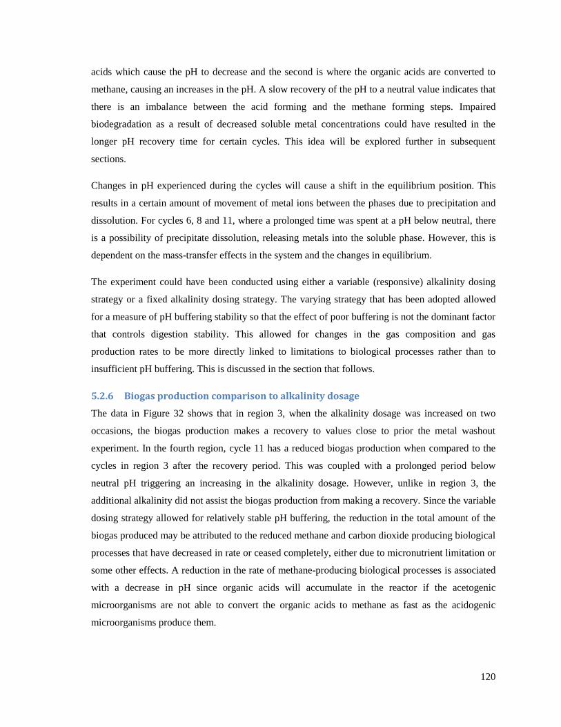
120

acids which cause the pH to decrease and the second is where the organic acids are converted to

methane, causing an increases in the pH. A slow recovery of the pH to a neutral value indicates that

there is an imbalance between the acid forming and the methane forming steps. Impaired

biodegradation as a result of decreased soluble metal concentrations could have resulted in the

longer pH recovery time for certain cycles. This idea will be explored further in subsequent

sections.

Changes in pH experienced during the cycles will cause a shift in the equilibrium position. This

results in a certain amount of movement of metal ions between the phases due to precipitation and

dissolution. For cycles 6, 8 and 11, where a prolonged time was spent at a pH below neutral, there

is a possibility of precipitate dissolution, releasing metals into the soluble phase. However, this is

dependent on the mass-transfer effects in the system and the changes in equilibrium.

The experiment could have been conducted using either a variable (responsive) alkalinity dosing

strategy or a fixed alkalinity dosing strategy. The varying strategy that has been adopted allowed

for a measure of pH buffering stability so that the effect of poor buffering is not the dominant factor

that controls digestion stability. This allowed for changes in the gas composition and gas

production rates to be more directly linked to limitations to biological processes rather than to

insufficient pH buffering. This is discussed in the section that follows.

5.2.6 Biogas production comparison to alkalinity dosage

The data in Figure 32 shows that in region 3, when the alkalinity dosage was increased on two

occasions, the biogas production makes a recovery to values close to prior the metal washout

experiment. In the fourth region, cycle 11 has a reduced biogas production when compared to the

cycles in region 3 after the recovery period. This was coupled with a prolonged period below

neutral pH triggering an increasing in the alkalinity dosage. However, unlike in region 3, the

additional alkalinity did not assist the biogas production from making a recovery. Since the variable

dosing strategy allowed for relatively stable pH buffering, the reduction in the total amount of the

biogas produced may be attributed to the reduced methane and carbon dioxide producing biological

processes that have decreased in rate or ceased completely, either due to micronutrient limitation or

some other effects. A reduction in the rate of methane-producing biological processes is associated

with a decrease in pH since organic acids will accumulate in the reactor if the acetogenic

microorganisms are not able to convert the organic acids to methane as fast as the acidogenic

microorganisms produce them.

121

5.2.7 Biogas production comparison to soluble metal concentration

To compare the total biogas produced from each cycle to the cycle at which a metal’s soluble

concentration started decreasing as predicted by the mass-balance speciation model, as well as to

the changing soluble concentrations as determined experimentally, the overlapping data may be

shown as follows:

Figure 33: Comparison of biogas production data with the experimental soluble metal concentration for Mg, Ca

and Fe and the model predicted cycle at which metal soluble concentration starts to decrease (in green boxes)

The soluble concentration of Ca, Mg, Cu and Mo are predicted to start decreasing from cycle 0.

From the experimental analysis (shown above in figure 33), the soluble concentrations for Ca and

Mg were found to decrease immediately after cycle 0. Literature indicates that Ca plays a role in

cell transport systems, osmotic balance and it aids flocculation while Mg, Cu and Mo have

enzymatic related functions (refer to table 3 and 4, section 2.3.2.2). Although the reported optimum

or stimulatory concentrations for these ions vary drastically (since each system will have its unique

ionic speciation) and some of them have been performed with other metals, they provide some

indication of what the metal concentration should be (table 2, section 2.3). The reported

0.0

2.0

4.0

6.0

8.0

10.0

12.0

14.0

16.0

-4 -2 0 2 4 6 8 10 12 14 16

Tota

l Bio

gas

Pro

du

ced

(lit

res)

So

lub

le M

eta

l Co

nce

ntr

atio

n (

mg/

l)

Cycle

Total Biogas Produced (litres) Mg (mg/l) Ca (mg/l) Fe (mg/l)

Ca, Mg, Cu, Mo Mn Zn, Co Ni Fe

122

optimum/stimulatory concentrations are relatively high; 120-1200 mg/l for Mg and 150-300 mg/l

for Ca. Mo has more modest reported stimulatory concentrations; from 0.05 mg/l to 2 mg/l.

Concentrations of less than the stimulatory or optimum concentrations would have therefore

resulted in less than optimum digestion and methane production. Consequently, it is possible that

the decrease in one or a combination of the soluble metal concentrations of Ca, Mg, Cu and Mo

would result in reduced biodegradation and lower methane production.

However, a reduction in the total biogas production only occurred in region two (regions dissected

by the purple lines as before), three cycles after these are predicted to washout. The metal phase

that most directly influences biological activity is the metals actually within the microorganisms.

When the soluble phase concentration decreases, the metals within the microorganisms will persist

for some time. Therefore, even if accurate predictions of the soluble concentrations are made, a lag

between the metal washout and the decrease in biological activity may be expected. A lag due to

the inclusion of other phases such as the organically bound phase is also possible. If the model by

taking into account these reasons for a lag period, had predicted the washout cycles to occur at a

later cycle, say three cycles later, then it would be possible to correlate the metal washout to the

total amount of biogas produced. The decreased biogas production observed in region 2 could be

attributed to the reduction in one or a more of the soluble concentrations of Ca, Mg Cu and Mo.

Employing similar reasoning, the decrease in region 4 can also be attributed to soluble metal

limitation. Zn is reported to have various enzyme related functions and to stimulate cell growth

while Co also has enzymatic functions including being a structural component of vitamin B12 (table

3 and 4, section 2.3.2.2). Although the model predicted that the Zn and Co soluble concentrations

will decrease from cycle 7, the experimentally determined sludge metal concentrations show little

change (Figure 26). Therefore, for Zn and Co, if the small soluble concentration that was in

equilibrium with the solid phases washed out and were not replenished due to some kinetic effects,

the decrease observed in region 4 could be partly attributed to a lack of these metals in the soluble

phase. The reduced biogas production in region 4 could also be attributed to reduced Mn and/or Ni

soluble concentrations. For Mn, an enzyme activator, the model predicts a reduction in soluble

metal concentration from cycle 3 (Figure 33 above) and experimentally, the sludge concentration

was observed to decrease (Figure 26). In addition to various enzyme related functions, Ni is

responsible for maintaining biomass (table 3 and 4, section 2.3.2.2). Although Ni was dosed to the

system at a concentration of 0.1 mg/l prior to the washout experiment, it was not detected in the

soluble analysis nor in the sludge analysis. This suggests that if the ICP-AES analysis was correct,

the Ni in this system has a poor sludge retention capacity and therefore will most likely occur in

123

very small sludge and soluble concentrations that are not detectable during ICP-AES analysis. Ni is

a metal which is not required in large concentrations; the reported optimum or stimulatory

concentrations for Ni are between 0.006 mg/l and 15 mg/l. Nevertheless, the model predicts that the

soluble concentration of Ni starts reducing from cycle 9.

Although the soluble concentrations for Fe were on the lower end of the range of reported

stimulatory/optimum concentrations (0.15 mg/l to 1000 mg/l, table 2, section 2.3) the reduced

biogas production in region 4 is most likely not due to Fe limitation, since experimentally, the

soluble concentration was found to decrease only after cycle 14. Therefore, the reduced biogas

production in region four may be attributed to the reduced soluble concentration in one or a

combination of the metals Mn, Zn, Co and Ni.

It was hypothesized that a mass balance chemical speciation-precipitation model can be used to

predict changes in soluble concentration such that changes biological activity can be predicted. The

results show that the effect of precipitation on metal dissolution can be modelled and a

correspondence to biological activity due to changes in soluble ion concentration was observed. In

most cases, order of magnitude effects were demonstrated by the model and the experimental data,

supporting the hypothesis. With further development of the model by including other phases such

as organically bound metals, the correlations and predictions are anticipated to improve. However,

at this stage the model is able to provide an improved understanding of the bioavailability of the

metals, as well as the ions responsible for sequestering the metals into the precipitate phase.

5.2.8 Validity of Model Assumptions

Due to the complexity of the chemical speciation system, the approach used in the development of

the model was a stage-wise approach. The model was therefore defined in the simplest way

possible; however, the long term objective of this research is to extend the model to more complex

forms where the simplifying assumptions in a simple model are not justified by the data. In most

cases, order of magnitude correlations were observed between the model and the experimental data.

The gap between the predictions and the data may be reduced by revisiting the key assumptions of

the model.

The sequential extraction in Experiment A (Figure 11) showed that although precipitation

sequestered metals (Al, Fe and Zn) to a large extent, organically bound metals was also a

significant phase that sequesters metals. Furthermore, the washout rate of the metals in Experiment

B was predicted to be more rapid than what the experimental analysis suggested. Since organically

bound metals are not considered to be very mobile, the exclusion of this phase in the model may

124

have contributed to the deviations. Metal in the adsorbed phase were also excluded from the model,

but the sequential extraction results indicate that a small, insignificant fraction of metals occur in

this phase (Figure 11). It is therefore recommended that for the next layer of model development,

the organically bound phase should be included.

As discussed earlier, in both Experiment A (section 5.1.4) and Experiment B (section 5.2.2), the

soluble metal concentrations of selected metals were generally higher than the model predicted

soluble concentrations. This could be attributed to mass transfer effects in the system which

prevented the system from reaching equilibrium. Although most precipitation reactions do not

reach equilibrium, the reactions tend towards equilibrium with less stable precipitates forming.

Furthermore, although a greater mass of precipitation would be anticipated at equilibrium, in reality

the amount of precipitation would not be drastically lower than the equilibrium amounts. This is

because the precipitation reactions would most likely have a high rate of formation in the initial

stages which later decreases over time. Therefore, although the equilibrium based model would

provide a reasonable indication of the speciation of the system, mass transfers effects would need to

be considered for a more accurate reflection of the system. In Experiment B (figures 20 and 23),

Mg, which had the majority of its ions in the soluble phase, had the best correlations between the

experimental data and the mode predictions (from Ca, Mg and Fe) while Fe, which had majority of

its ions in solid related phases, did not correlate as well as Mg or Ca. This suggests that for those

metals which are mostly associated with rapid inorganic complexation reactions, better correlations

to an equilibrium model would be observed than for those metals that are mostly associated with

slower precipitation or organic complexation reactions.

The electrical potential and reduction/oxidation reactions of the system were not taken into account

by the model, although it was assumed that all the sulphate dosed to the system was reduced to

sulphide. This is a sensible assumption since under anaerobic conditions, the redox potential is low

and the reduction of sulphate to sulphide is a biologically catalysed reaction which would near

equilibrium. However, the electrical potential of a system is one of the factors that determine the

state in which a metal ion will occur in the system. In Experiment B, although Ni was dosed to the

system prior to the metal washout experiment and precipitation was predicted by the model, but the

ICP-AES analysis of the sludge or the supernatant samples did not show the presence of Ni,

suggesting that the ions may have occurred in the soluble phase and were continuously washed out

of the system. This may be due to a number of reasons, one of which being that although the Ni was

predicted to precipitate, the actual redox potential of the system was not as low as assumed and

therefore, not favourable for Ni precipitation. Bearing this in mind, it may be of value to check the

125

electrical potential of the system under investigation against the predicted electrical potential. If

there are vast differences between the two values, it would be recommended to revisit this

assumption so that the model may better predict the conditions under which precipitation will

occur.

5.2.9 Dosing Strategy

The model together with the experimental analysis was able to provide an understanding of the

speciation of the metals in the system, leading to recommendations to improve the micronutrient

dosing by either increasing the bioavailability or by reducing the dosage of ineffective metals.

Throughout the discussion, recommendations for the various metals were made. It was apparent

from Figure 25 that since a large percentage of Ca was being washed out of the system prior to the

metal washout experiment, there was most likely a large reservoir of Ca in the sludge phase within

the reactor. Therefore, reducing the Ca dosage to the feed may be investigated. For Mg, the model

and the experimental analysis show that majority of the ions are in the soluble phase (Figures 19

and 20). Since the reported stimulatory concentrations for Mg are high (between 120 and 1200 mg/l

(table 2, section 2.3) an increase in the Mg dosage concentration to enhance the digestion may be

investigated.

Figures 26 and 28 showed that Zn has a very high sludge retention capacity that did not change

even when the metal dosage was stopped. Furthermore, Co, Fe, and Cu also displayed minimal

changes in the sludge concentration during the washout experiment. These observations were also

supported by findings from various studies. Therefore, it is recommended that the dosage

concentration for Zn should be reduced and for all the metals including Zn, an intermittent dosing

strategy may be employed.

Figures 18 and 19 show that although the majority of the metals were predicted to be sequestered

within sulphide precipitates, only about 10% of the sulphide ions were predicted to occur in the

soluble phase. This suggests that the sources of sulphide (dosed as sulphates) are unnecessarily high

in the system and that this can be reduced. Co, Cu and Fe are metals that have extremely low Ksp

values with their sulphide precipitates. Therefore, attempting to increase the bioavailability by

increasing the dosage concentration will most likely not work. For these ions, a dosage strategy that

increases the solubility of the metals should be investigated. The use of weak chelating agents, such

as yeast, is one such method which has been demonstrated to increase the bioavailability of Co and

Ni (Gonzalez-Gil et al., 2003). Although yeast extract is already dosed to the system, an increase in

the dosage concentration should be investigated.

126

Ni was dosed to the reactors at a low concentration (0.1 mg/l), and the ions were not detected in the

soluble or the sludge metal analysis (Figures 25 and 26). Furthermore, Ni was predicted to occur in

very small soluble concentrations (approximately 4 x 10-10

mg/l shown in figure 22) and reported

stimulatory concentrations for Ni, although varied, go up to 15 mg/l (table 2, section 2.3). Although

the absence of Ni from the ICP-AES analysis (both sludge and supernatant) could have been due to

interferences during the analysis resulting in inaccurate ICP-AES data, an increase in the Ni dosing

concentration should be investigated. In addition to possibly enhancing the anaerobic

biodegradation, a higher dosage concentration may increase the likelihood of detecting the metal

during ICP-AES analysis.

The recommendations above will be applicable for the system under investigation or similar

systems anaerobically treating FTRW. However, the mass-balance speciation model is a tool that

may be applied to any other system. This, together with discerning experimental analysis would

provide valuable information on the speciation of metals in a system. This in turn may be used to

develop a prudent micronutrient dosing strategy without having to perform numerous dosing

response experiments.

127

6. Conclusions and Recommendations

In this study it was hypothesized that a combined mass balance and chemical speciation model

could be used to predict the soluble metal ion concentration such that changes in methanogenic

activity, in response to changes in metal ion concentration, could be predicted. This was undertaken

by investigating the influence of precipitation on bioavailability and examining the extent to which

precipitation can sequester metals into forms that are not bioavailable and the extent to which this

sequestration can describe biological effects.

The sequential extraction of the sludge in Experiment A showed that for Al, Zn and Fe, majority of

the metals occurred within two significant phases, namely, the precipitates and the organically

bound phase. The fraction of metals in the adsorbed phase was small. Mg was found to have a large

portion in the bioavailable phase. For trace metals Cu, Cr and Ni, the sequential extraction analysis

was unsuccessful since these metals occur in such small concentrations that when separated into the

different metal phases, the concentrations are difficult to detect during the ICP-AES analysis.

Nonetheless, the results suggested that a significant portion of Cr lies within the organically bound

phase. Precipitation was found to sequester metals to a large extent making them non-bioavailable.

However, the organically bound metals were a significant portion of sequestered metals.

For the anaerobic system treating FTRW (Experiment B), a large degree of sequestration of Co, Cu,

Ni, Zn, Fe and Mo by sulphide precipitates was predicted by the model. This was not unexpected

since these metals have small Ksp values for sulphide precipitates. This was supported by

experimental analysis as the metals Co, Cr, Cu, Mn and Zn were too small to be detected in the

soluble metal analysis, but were found in the solid phase analysis. This is problematic in terms of

metal bioavailability since only a small soluble concentration will be in equilibrium with the

predicted precipitates. This is regardless of the presence of other metal phases since the Ksp value

controls the soluble concentration which in turn dictates the amount of metals sequestered by the

different phases. Since the sludge is the chief source of metals, it is recommended that, for future

experimental work, a more accurate method should be developed for sampling and analysing the

sludge, and direct measurements should be used where possible.

At the current stage of the model development, only the precipitate phase was considered as a form

of metal sequestration. In Experiment A, although there were reasonable correlations observed,

deviations between the model predicted and the experimentally determined metal soluble

concentrations were found; the experimentally determined soluble concentrations were higher than

the predicted values. There are three possible reasons for these differences. The first is that there

128

was an experimental error with the analysis. The second is that the assumption that the system was

at equilibrium does not hold, and as such, there were kinetic effects in the system that needed to be

accounted for. The third reason could be that the two phase (soluble and precipitate) model was

insufficient to accurately predict the soluble concentrations and the inclusion of an additional phase

such as the organically bound phase would provide a better correlation. Since the soluble

concentration of a metal in the reactor will dictate the amount of metal ions in the other phases

(according to equilibrium/formation constants), the model should predict the soluble concentrations

fairly well if the system is at equilibrium. Since the soluble concentrations were higher than the

model predicted values, the deviations were most likely due to kinetic effects in the system that

hindered complete precipitation from occurring. It is also possible that a portion of the metal ions

in the aqueous phase were present as chelates. Attempts should thus be made to further develop and

improve the model by revisiting these assumptions in the next layer of development.

The washout experiment and monitoring of biological processes in Experiment B allowed testing

whether changes in biological activity in response to changes in the soluble metal concentrations

could be predicted by the mass-balance equilibrium speciation model. The deviations during the

washout experiment between the soluble concentrations determined experimentally (Mg, Ca and

Fe) and the model predicted concentrations may also be attributed to mass transfer effects, to the

absence of other phases that sequester metals in the model or to a combination of these effects. If

mass transfer effects were at play in the system, sufficient dissolution of precipitates to replenish

the lost soluble concentrations from the washout would not occur, causing the model to over-

predict the rate at which metals were washed out of the system. The presence of other metal solid

phases such as organically bound metals would also cause the model to predict a different rate of

soluble metal washout since the movement of metals from these phases to the soluble phase is

dependent on a number of other effects. In the case of organically bound metals, which was found

to be a significant phase that sequesters metals, the formation of stable organic substances that do

not easily release metals would cause the model to over-predict the rate of soluble metal washout.

However, at this stage, it is not clear which of the two effects are responsible for the differences or

whether it is a combination of these effects. It is also interesting to note that from the three metal

ions (Mg, Ca and Fe) that were determined experimentally during the washout experiment, Mg,

which has majority of its ions in the soluble phase, had the best correlations while Fe, which has

majority of its ions in solid related phases, did not correlate as well as Mg or Ca.

When comparing the biogas production from before the washout experiment to 12 cycles after, the

biogas production decreased by 43%. In between these 12 cycles there was a recovery period

129

observed where the alkalinity dosage was increased to overcome acid accumulation and the biogas

production recovered to about 90% of the production prior to the metal washout experiment. This

type of response has been observed before in similar micronutrient limiting studies where after the

recovery period, the measure of biological activity decreased further than the initial period of

decline.

The varying dosage strategy used for pH control for some measure of pH stability consequently

allowed for other effects such as micronutrient limitation to dictate effects for digestion stability.

Although, this approach indicates that the commencement of severe instability and digestion failure

from stable operating conditions may not always be clearly seen, resulting changes in biogas

production and composition are more directly linked to limitations in biological processes due to

micronutrient limitation.

A lag between the soluble metal washout and a possible decrease in biological activity is expected

since the metals already within the microorganisms will persist for some time. Additionally, the

inclusion of other phases such as the organically bound phase may result in a slower reduction in

the soluble concentration than predicted by the model. When comparing the cycles where a

decreased biogas production was observed to the decreases in soluble metal concentration obtained

experimentally as well as those predicted by the model, and concurrently taking into account a lag

period, certain correlations were found. From the first cycle without micro-metal dosage, the

soluble concentrations determined experimentally for Ca and Mg started decreasing while the Cu

and Mo soluble concentrations were predicted to decrease. Therefore, a decrease in one or a

combination of these metals may have resulted in the initial decline in biogas production. During

the recovery period, the soluble concentrations of Zn, Co and Ni were predicted to start decreasing

while the sludge metal concentration for Mn was also found to decrease, suggesting that the soluble

concentration was decreasing. A decrease in one or a combination of these metals most likely

resulted in the second decline observed in the biogas production.

Since there was a correlation between the times at which metals washed out of the reactor and the

observed changes in the biogas production, it provided strong evidence that washout of metals had

a direct negative influence on anaerobic activity. Although the model formulation proposed made

use of significant simplifications, an agreement between predicted metals washout and reduction in

anaerobic activity was observed, indicating that this is a promising new approach for understanding

and modelling bioavailability of metals in anaerobic digestion. Furthermore, the model together

130

with the experimental analysis was able to provide an understanding of the speciation of the metals

in the system such that recommendations to improve the micronutrient dosing were made.

The high soluble metal washout rate for Ca prior to the actual washout experiment suggests that

there is a large reservoir of Ca in the reactor and that the Ca dosage to the system may be reduced.

Zn was found to have a high sludge retention capacity. Furthermore, Co, Fe, and Cu also displayed

minimal changes in the sludge concentration during the washout experiment. Therefore, it is

recommended that for Zn, the dosage concentration should be reduced and for all the metals

including Zn, an intermittent dosing strategy may be employed. Co, Cu, Fe and Ni were found or

predicted to occur in very small soluble concentrations most likely due to the small Ksp values of

their sulphide precipitates. For these metals, an increase in the yeast extract dosage concentration or

dosing another weak chelating agent should be investigated to try and increase their soluble

concentration.

The recommendations above will mostly be applicable for this system under investigation or

similar systems treating FTRW anaerobically. However, the mass-balance speciation model

together with discerning experimental analysis would provide valuable information on the

speciation of metals in any other system which may be used to develop a prudent micronutrient

dosing strategy.

131

7. References

Allsop, P.J., Chisti, Y., Moo-Young, M., &Sullivan, G.R., 1993. Dynamics of phenol

degradation by Pseudomonas putida. Biotechnology and Bioengineering, 41, 572-580.

APHA, 1989. Standard Methods for the examination of water and wastewater.17th Ed.

Washington DC: American Public Health Association.

APHA, 1996. Standard Methods for the examination of water and wastewater.17th Ed.

Washington DC: American Public Health Association.

Aquino, S.F. and Stuckey, D.C., 2007. Bioavailability and Toxicity of Metal Nutrients

during Anaerobic Digestion. Journal of Environmental Engineering 133 (1).

Beaudoin, G., 2000. Acicular sphalerite enriched in Ag, Sb, and Cu embedded within

colour-banded sphalerite from the Kokanee Range, British Columbia, Canada. The

Canadian Mineralogist, 38, 1387-1398.

Bhattacharya, S.K.k, Uberoi, V., Madura, R.L., & Haghighi-Podeh, M.R., 1995. Effect of

cobalt on methanogenesis. Environmental Technology, 16(3), 271-278.

Björnsson, L., Mattiasson, B., & Henrysson, T., 1997. Effects of support material on the

pattern of volatile fatty acid accumulation at overload in anaerobic digestion of semi-solid

waste. Applied Microbiology and Biotechnology, 47(6), 640-644.

Borja, R., Sánchez, E., and Weiland, P., 1996. Influence of ammonia concentration on

thermophilic anaerobic digestion of cattle manure in upflow anaerobic sludge blanket

(UASB) reactors. Process Biochemistry, 31(5), 477-483.

Burgess, J. E., Quarmby, J., & Stephenson, T., 1999. Role of micronutrients in activated

sludge-based biotreatment of industrial effluents. Biotechnology Advances, 17(1), 49-70.

Callendar, I.J., and Barford, J.P., 1983. Precipitation, chelation and availability of metals as

nutrients in anaerobic digestion. II. Biotechnology and Bioengineering, 25(8), 1959-1972.

Chen, Y., Cheng, J. J., & Creamer, K. S., 2008. Inhibition of anaerobic digestion process:

A review. Bioresource Technology, 99(10), 4044-4064.

Chisti, Y., 1998. Pneumatically agitated bioreactors in industrial and environmental

bioprocessing: Hydrodynamics, hydraulics and transport phenomena. Appl. Mech. Rev., 51,

33-112.

Coetzee, P.P., 1993. Determination and speciation of heavy metals in sediments of the

Hartbeespoort Dam by sequential chemical extraction. Water SA, 19, 291.

Colleran, E., Finnegan, S., and Lens, P., 1995. Anaerobic treatment of sulphate-containing

waste streams. Antonie van Leeuwenhoek, 67(1), 29-46.

132

Deer, W.A., Howie, R.A., Zussman, J., 1996. The Rock Forming Minerals. Essex, England:

Pearson Education Limited.

Drobner, E., Huber, H., Wachtershauser, G., Rose, D., & Stetter, K.O., 1990. Pyrite

formation linked with hydrogen evolution under anaerobic conditions. Nature, 346, 742-

744.

Dry, M. E., 2002. The Fischer-Tropsch process: 1950-2000. Catalysis Today, 71(3-4), 227-

241.

Environmental Protection Agency (EPA), 2007. Framework for Metals Risk Assessment.

Risk Assessment Forum, US Environmental Protection Agency.

Espinosa, A., Rosas, L., Ilangovan, K. & Noyola, A., 1995. Effect of trace metals on the

anaerobic degradation of volatile fatty acids in molasses stillage. Water Science and

Technology, 32(12), 121-129.

Fang, H.H.P., and Hui, H.H., 1994. Effect of heavy metals on the methanogenic activity of

starch-degrading granules. Biotechnology Letters, 16(10), 1091-1096.

Fermoso, F.G., 2008. Metal supplementation to anaerobic granular sludge bed reactors:

An environmental approach. PhD. Thesis, Wageningen University, The Netherlands.

Fermoso, F. G., Bartacek, J., Chung, L. C., & Lens, P., 2008a. Supplementation of cobalt to

UASB reactors by pulse dosing: CoCl2 versus CoEDTA2- pulses. Biochemical

Engineering Journal, 42(2), 111-119.

Fermoso, F. G., Bartacek, J., Jansen, S., & Lens, P. N. L., 2009. Metal supplementation to

UASB bioreactors: from cell-metal interactions to full-scale application. Science of The

Total Environment, 407(12), 3652-3667.

Fermoso, F.G., Bartacek, J., Manzano, R., Van Leeuwen, H.P. and Lens, P.N.L., 2010.

Dosing of anaerobic granular sludge bioreactors with cobalt: Impact of cobalt retention on

methanogenic activity. Bioresource Technology 101 (24) 9429-9437.

Filgueiras, A.V., Lavilla, I., and Bendicho, C., 2002. Chemical sequential extraction for

metal partitioning in environmental solid samples. Journal of Environmental Monitoring 4

(6), 823-857.

Franta, J., Wilderer, P.A., Miksch, K., & Sykora, V., 1994. Effects of operation conditions

on advanced COD removal in activated sludge systems. Water Science and Technology,

27(7), 189-192.

Fränzle, S., and Markert, B., 2002. The Biological System of the Elements (BSE)--a brief

introduction into historical and applied aspects with special reference on "ecotoxicological

133

identity cards" for different element species (e.g. As and Sn). Environmental Pollution,

120(1), 27-45.

Giammar, D.E., Bruant, R.G., Peters, C.A., Forsterite dissolution and magnesite

precipitation at conditions relevant for deep saline aquifer storage and sequestration of

carbon dioxide. Chemical Geology, 217, 257-276.

Gonzalez, J.F., and Hu, W.S., 1991. Effect of glutamate on the degradation of

pentachlorophenol by Flavobacterium spp. Applied Microbiology and Biotechnology,

35(1), 100-104.

Gonzalez-Gil, G., Jansen, S., Zandvoort, M. H., and van Leeuwen, H. P., 2003. Effect of

yeast extract on speciation and bioavailability of nickel and cobalt in anaerobic bioreactors.

Biotechnology and Bioengineering, 82(2), 134-142.

Gramp, J.P., Sasaki, K., Bigham, J.M., Karnachuk, O.V., & Tuovinen, O.H., 2006.

Formation of Covellite (CuS) under biological sulphate-reducing conditions.

Geomicrobiology Journal, 23(8), 613-619.

Gribble, C.D., 1988. Economic grouping of minerals according to elements. Rutley’s

Elements of Minerology, 150-210.

Guibaud, G., Bordas, F., Saaid, A., D'Abzac, P., and Van Hullebusch, E., 2008. Effect of

pH on cadmium and lead binding by extracellular polymeric substances (EPS) extracted

from environmental bacterial strains. Colloids and Surfaces B: Biointerfaces, 63(1), 48-54.

Hanrahan, G., 2010. Modelling of Pollutants in Complex Environmental Systems, Vol 2.

ILM Publications, UK.

Harada, H., Uemura, S., and Monomoi, K., 1994. Interactions between sulphate-reducing

bacteria and methane producing bacteria in UASB reactors fed with low strength wastes

containing different levels of sulphate. Water Research,28(2), 355-367

Heipieper, H.J., Weber, F.J., Sikkema, J., Kewelch, H., and de Bont, J.A.M., 1994.

Mechanisms of resistance of whole cells to toxic organic solvents. Trends in

Biotechnology, 12(10), 409-415.

Hendriksen, H.V., Larsen, S., & Ahring, B.K., 1992. Influence of supplemental carbon

sources on the anaerobic dechlorination of pentachlorophenol in granular sludge. Applied

and Environmental Microbiology, 58(1), 365-370.

Hilton, B.L. and Oleszkiewicz, J.A., 1988. Sulfide-Induced Inhibition of Anaerobic

Digestion.

Journal of Environmental Engineering, Vol. 114, No. 6, November/December 1988, pp.

1377-1391.

http://cedb.asce.org/cgi/WWWdisplay.cgi?168569

http://cedb.asce.org/cgi/WWWdisplay.cgi?168569

134

Hoban, D.J., and Van den berg, L., 1979. Effect of iron on conversion of acetic acid to

methane during methanogenic fermentations. Journal of Applied Bacteriology, 47(1), 153-

159.

Huber, H., Filella, M., and Town, R.M., 2002. Computer modelling of trace metal ion

speciation: practical implementation of a linearcontinuous function for complexation by

natural organic matter. Computers & Geosciences 28,587-596.

Hyun, S.P., and Hayes, K.F., 2009. Feasibility of using in situ FeS precipitation for TCE

degradation. Journal of Environmental Engineering, 135, 1009-1014.

Ilangovan, K., & Noyola, A., 1993. Availability of micronutrients during anaerobic

digestion of molasses stellage using an upflow anaerobic blanket (UASB) reactor.

Environmental Technology, 14(8), 795-799.

Ivanov, A.I., 2008. Exocytosis and Endocytosis. Totowa, NJ: Human Press.

Jackson-Moss, C.A., and Duncan, J.R., 1991. The effect of aluminum on anaerobic

digestion. Biotechnology Letters, 13(2), 143-148.

Jackson-Moss, C.A., Duncan, J.R., and Cooper, D.R., 1989. The effect of calcium on

anaerobic digestion. Biotechnology Letters, 11(3), 219-224.

Jansen, S., Gonzalez-Gil, G., & van Leeuwen, H.P., 2007. The impact of Co and Ni

speciation on methanogenesis in sulfidic media- Biouptake versus metal dissolution.

Enzyme and Microbial Technology, 40, 823-830.

Kayhanian, M., 1999. Ammonia Inhibition in High-Solids Biogasification: An Overview

and Practical Solutions. Environmental Technology, 20(4), 355 - 365.

Kayhanian, M. and Rich, D., 1995. Pilot-scale high solids thermophilic anaerobic digestion

of municipal solid waste with an emphasis on nutrient requirements. Biomass and

Bioenergy 8 (6) 433-444.

Kelly, C.R., and Switzenbaum, M.S., 1984. Anaerobic treatment: Temperature and nutrient

effects. Agricultural Wastes, 10(2)., 135-154.

Kroeker, E. J., Schulte, D. D., Sparling, A. B., and Lapp, H. M., 1979. Anaerobic

Treatment Process Stability. Journal (Water Pollution Control Federation), 51(4), 718-

727.

Kroiss, H. and Zessner, M., 2001. Wastewater treatment and sludge disposal- What are the

challenges? European Council of Applied Sciences and Engineering.

Kugelman, I.J., and Chin, K.K., 1971. Toxicity, synergism and antagonism in anaerobic

treatment processes. Adv. Chem. Ser., 105, 55.

135

Kugelman, I.J., and McCarty, P.L., 1964. Cation toxicity and stimulation in anaerobic

waste treatment. Journal of Water Pollution Control Federation, 37(1), 97-116.

Labrenz, M., Druschel, G.K., Thomsen-Ebert, T., Gilbert, B., Welch, S.A., Kemner, K.M.,

Logan, G.A., Summons, R.E., De Stasio, G., Bond, P.L., Lai, B., Kelly, S.D., and Banfield,

J.F., 2000. Formation of Sphalerite (ZnS) deposits in natural biofilms of sulfate-reducing

bacteria. Sciencemag, 290 no. 5497, 1744-1747.

Leahy, J. G., and Colwell, R. R., 1990. Microbial degradation of hydrocarbons in the

environment. Microbiol. Mol. Biol. Rev., 54(3), 305-315.

Lees, C., 2013. Dynamic Modeling of Anaerobic Digestion of Fischer-Tropsch Reaction

Water: Different Approaches to Physico-chemical Modeling. PhD Thesis, University of

Kwa-Zulu Natal.

Lemmer, H., and Nitschke, L., 1994. Vitamin content of four sludge fractions in the

activated sludge waste water treatment process. Water Research, 28(3), 737-739.

Lin, C., and Chen, C., 1999. Effect of heavy metals on the methanogenic UASB granule.

Water Research, 33(2), 409-416.

Lin, C., and Chen, C., 1999. Effect of heavy metals on the methanogenic UASB granule.

Water Research, 33(2), 409-416.

Manning, J. And Grow, W.R., 1997. Inductively Coupled Plasma - Atomic Emission

Spectrometry. The Chemical Educator 2 (1) 1-19.

Martin, T.D., Brockhoff, C.A. & Creed, J.T., 1998. Trace elements in water, solids, and

biosolids by inductively coupled plasma-atomic emission spectrometry. EPA Method 200.7

Revision 5.

Massé, D.I. and Masse, L., 2000. Treatment of slaughterhouse wastewater in anaerobic

sequencing batch reactors. Canada Agricultural Engineering 42 ( 3).

McCarty, P.L., 1964. Anaerobic waste treatment fundamentals. Public Works 95 (9), 107–

112.

Morel, F.M.M., and Hering, J.G., 1993. Principles and Applications of Aquatic Chemistry.

England: John Wiley & sons.

Musvoto, E.V., Wentzel, M.C. and Ekama, G.A., 2000. Integrated chemical-physical

processes modelling-II. Simulating aeration treatment of anaerobic digester supernatants.

Water Research, 34(6), 1868-1880.

Nordstrom, D.K., 1996. Trace metal speciation in natural waters: Computational vs.

Analytical. Water, Air and Soil Pollution 9, 257-267.

136

Osuna, M.B., Iza, J., Zandvoort, M., and Lens, P.N.L., 2003. Essential metal depletion in

an anaerobic reactor. Water Sci. Technol., 48(6), 1-8.

Owen, W. F., Stuckey, D. C., Healy Jr, J. B., Young, L. Y., & McCarty, P. L., 1979.

Bioassay for monitoring biochemical methane potential and anaerobic toxicity. Water

Research, 13(6), 485-492.

Paulo, P.L., Jiang, B., Stams, A.J.M., & Lettinga, G., 2004. Effect of Co on the anaerobic

thermophilic conversion of methanol. Biotechnology and Bioengineering, 85(4), 434-441.

Peijnenburg, W.J.G.M., and Jager, T., 2003. Monitoring approaches to assess

bioaccessibility and bioavailability of metals: Matrix issues. Ecotoxicology and

Environmental Safety, 56, 63-77.

Percheron, G., Bernet, N., & Moletta, R., 1997. Start-up of anaerobic digestion of sulphate

wastewater. Bioresource Technology, 61, 21-27.

Sanchez-Roman, M., McKenzie, J.A., Wagener, A.D.L.R, Rivadeneyra, M.A.,

Vasconcelos, C., 2009. Presence of sulphate does not inhibit low-temperature dolomite

precipitation. Earth and Planetary Science Letters, 285, 131-139.

Sauve, S., McBride, M.B., & Hendershot, W.H., 1995. Ion-selective electrode

measurements of copper (II) activity in contaminated soils. Arch. Environ. Contam.

Toxicol. 29. 373-379.

Scherer, P., and Sahm, H., 1981. Influence of sulphur-containing compounds on the growth

of Methanosarcina bakeri in a defined medium. Eur. J. Appl. Microbiol. Biotechnol. 12(1),

28-35.

Schmidt, J.E., and Ahring, B.K., 1993. Effects of magnesium on thermophilic acetate-

degrading granules in upflow anaerobic sludge blanket (UASB) reactors. Enzyme and

Microbial Technology, 15(4), 304-310.

Seely, O., 2007. Selected Solubility Products and Formation Constants at 25°C, [online].

Available at www.csudh.edu/oliver/chemdata/data-ksp.htm. [Accessed 28 February 2014].

Sharma, J., and Singh, R., 2001. Effect of nutrients supplementation on anaerobic sludge

development and activity for treating distillery effluent. Bioresource Technology, 79, 203-

206.

Shelton, D.R. and Tiedje, J.M., 1984. General method for determining anaerobic

biodegradation potential. Applied and Environmental Microbiology 47 (4) 850-857.

Sikkema, J., de Bont, J.A., and Poolman, B., 1994. Interactions of cyclic hydrocarbons with

biological membranes. The Journal of Biological Chemistry 269(11), 8022-8028.

http://www.csudh.edu/oliver/chemdata/data-ksp.htm

137

Simkiss, K. And Taylor, G., 1995. Transprot of Metals Across Membranes. Metal

Speciation and Bioavailability in Aquatic Systems, 3, 1-44.

Singleton, J., 1994. Microbial metabolismof xenobiotics: Fundamental and applied

research. J. Chem. Techno. Biotechnol, 59, 9-23.

Sohnel, O., and Garside, J., 1992. Precipitation: Basic Principles and Industrial

Applications. Oxford: Butterworth-Heinemann.

Soto, M., Mendez, R., and Lema, J.M., 1993. Methanogenic and non-methanogenic activity

tests: theoretical basis and experimental setup. Water Research, 27(8), 1361-1376.

Speece, R.E., 1996. Anaerobic Biotechnology for industrial wastewaters. Nashville,

Tennessee: Archae Press.

Sterritt, R.M., and Lester, J.N., 1980. Interaction of heavy metals with bacteria. The Science

of the Total Environment, 14(1), 5-17.

Steyer J.P., Bouvier J.C., Conte T., Gras P. and Sousbie P., 2002. Evaluation of a four year

experience with a fully instrumented anaerobic digestion process, Water Science and

Technology, 45 (4-5) 495-502.

Steyer, J.P., Bernard, O., Batstone, D.J. and Angelidaki, I., 2006. Lessons learnt from 15

years of ICA in anaerobic digesters. Water Science and Technology, 53 (4-5) 25-33.

Stover, R.C., Sommers, L.E., & Silviera, D.J., 1976. Evaluation of metals in wasterwater

sludge. Journal Water Pollution Control Federation, 48(9), 2165-2175.

Stumm, W. and Morgan, J.J., 1996.Chemical Equilibria and Rates in Natural Waters. 3rd

Ed. Wiley.

Sunda, W.G., and Huntsman, S.A., 1998. Processes regulating cellular metal accumulation

and physiological effects: Phytoplankton as model systems. Science of the Total

Environment, 219, 165-181.

Sung, S., and Dague, R.R., 1995. Laboratory studies on the Anaerobic Sequencing Batch

Reactor. Water Environment Research, 67(3), 294-301.

Tessier, A., Cambell, P.G.C., & Bisson, M., 1979. Seuential extraction procedure for the

speciation of particulate trace metals. Analytical Chemistry, 51(7), 844-851.

Tessier, A., and Turner, D.R., 1995. Metal Speciation and Bioavailability in Aquatic

Systems. West Sussex, England: John Wiley.

Tipping, E., Lofts, S. and Lawlor, A.J., 1998. Modelling the chemical speciation of trace

metals in the surface waters of the Humber system. The Science of the Total Environment

210/211, 63-77.

138

Turner, A., and Mawji, E., 2005. Hydrophobicity and reactivity of trace metals in the low-

salinity zone of a turbid estuary. Limnol. Oceanogr., 50(3), 1011-1019.

Vallee, B.L., and Ulner, D.D., 1972. Biochemical effects of mercury, cadmium and lead.

Annual review of Biochemistry, 41(10), 91-128.

Van der Veen, A., Fermoso, F. G., and Lens, P. N. L., 2007. Bonding Form Analysis of

Metals and Sulfur Fractionation in Methanol-Grown Anaerobic Granular Sludge.

Engineering in Life Sciences, 7(5), 480-489.

Van Hullebusch, E.D., Utomo, S., Zandvoort, M.H. and Lens, P.N.L., 2005. Comparison of

three sequential extraction procedures to describe metal fractionation in anaerobic granular

sludges. Talanta 65 549-558.

Van Zyl, P.J., 2008. Anaerobic digestion of Fischer-Tropsch reaction water- Submerged

membrane anaerobic reactor design, performance evaluation & modelling. Ph D.

University of Cape Town.

Van Zyl, P.J., Lees, C.M., Brouckaert, C.J., Ekama, G.A. and Foxon, K.M., 2012. Dynamic

modeling of anaerobic digestion of Fischer-Tropsch reaction water: Different approaches to

physio-chemical modeling. Wisa Wastewater Treatment 1129, 414.

Venkataramani, E.S., and Ahlert, R.C., 1985. Role of cometabolism in biological oxidation

of synthetic compounds. Biotechnology and Bioengineering, 27, 1306-1311.

Vink, B.W., 1896. Stability relations of malachite and azurite. Mineralogical Magazine, 50,

41-47.

Wadley, S., and Buckley, C.A., 1997. Chemical speciation self-study work manual;

Pollution Research Group, University of Kwa-Zulu Natal.

Wahal, S., 2010. Nutrient utilization from anaerobic digester effluent through algae

cultivation.PhD Thesis, Utah State University, Utah.

Weiland, P., 2010. Biogas production: current state and perspectives. Applied Microbiology

and Biotechnology, 85(4), 849-860.

Wilkie, A., Goto, M., Bordeaux, F.M., & Smith, P.H., 1986. Enhancement of anaerobic

methanogenesis from napiergrass by addition of micronutrients. Biomass, 11(2), 135-146.

Wood, D. K., and Tchobanoglous, G., 1975. Trace Elements in Biological Waste

Treatment. Journal (Water Pollution Control Federation), 47(7), 1933-1945.

Worms, I., Simon, D.F., Hassler, C.S., & Wilkinson, K.J., 2006. Bioavailability of trace

metals to aquatic microorganisms: importance of chemical, biological and physical

processes on biouptake. Biochimie, 88, 1721-1731.

139

Wray, J.L., and Daniels, F., 1957. Physical and inorganic chemistry. Journal of American

Chemical Society, 79(9), 2031-2034.

Yu, H.Q., Tay, J.H., & Fang, H.P., 2001. The roles of calcium in sludge granulation during

UASB reactor start-up. Water Research, 35(4), 1052-1060.

Zaiat, M., Rodrigues, J.A.D, Ratusznei, S.M., de Camargo, E.F.M and Borzani, W., 2001.

Anaerobic sequencing batch reactors for wastewater treatment: a developing technology.

Applied Microbioogicall Biotechnology 55 29-35.

Zandvoort, M. H., Geerts, R., Lettinga, G., & Lens, P. N. L., 2002. Effect of long-term

cobalt deprivation on methanol degradation in a methanogenic granular sludge bioreactor.

[Article]. Biotechnology Progress, 18(6), 1233-1239.

Zandvoort, M.H., Geerts, R., Lettinga, G., & Lens, P.N.L., 2003. Methanol degradation in

granular sludge reactors at sub-optimal metal concentrations: role of iron, nickel and cobalt.

Enzyme and Microbial Technology, 33, 190-198.

Zandvoort, M. H., Gieteling, J., Lettinga, G., & Lens, P. N. L., 2004. Stimulation of

Methanol Degradation in UASB Reactors: In Situ Versus Pre-Loading Cobalt on

Anaerobic Granular Sludge. Biotechnology and Bioengineering, 87 (7) 897-904.

Zufiaurre, R., Olivar, A., Chamorro, P., Nerin, C., & Callizo, A., 1998. Speciation of

metals in sewage sludge for agricultural uses. The Analyst, 123, 255-259.

140

8. Appendix A-List of Micro-nutrient recipes from Literature

There are numerous references that provide nutrient medium recipes for anaerobic microorganisms.

These differ with regards to composition as well as the concentration of the metals. It should be

kept in mind that although these systems would have similar types and strains of bacteria, they are

still inherently different courtesy of different reactors, substrates and operating conditions. The

table that follows provides some of these recipes together with a description of the systems they

were supplemented to:

141

Table 19: Nutrient Recipes used in Literature and their values compared to the recipe used by Sasol

Referance Reactor

Type

Substrate Feed COD/OLR Element Concentration(mg/l) Compound Dosed Compare

to Sasol

Owen et al., 1979 Batch Pure Cellulose < 2 g/l N 0.008 NH4Cl, (NH4)2HPO4 3.079E-05

(Without vitamins) P 0.017 (NH4)2HPO4 0.0003

K 0.614 KCl 0.0047

S 0.060 Na2S.9H2O 0.0026

Ca 0.061 CaCl2.2H2O 0.0205

Mg 0.194 MgCl2.6H2O 0.0149

Fe 0.094 FeCl2.4H2O 0.0085

Cu 0.001 CuCl2.2H2O 0.0060

Zn 0.001 ZnCl2 0.0027

Mn 0.005 MnCl2.4H2O 0.0249

Mo 0.001 Na2MoO4.2H2O 0.1300

Co 0.007 CoCl2.6H2O 0.3344

B 0.001 H3BO3 0.0997

Speece, 1996 pH-Stat Acetate 30-60 g/l.d N 100.000 mostly as chloride 0.4000

Reactor

P 4.000 salts 0.0667

K 100.000

0.7692

S 10.000

0.4348

Ca 5.000

1.6667

Mg 1.000

0.0769

Fe 1.000

0.0909

Zn 0.100

0.3030

Ni 0.200

2.0000

142

Co 0.100 5.0000

Zandvoort, 2003 UASB Methanol 2.6-7.8 g/l.d Fe 562.000 FeCl2.4H2O 51.0909

Cu 14.000 CuCl2.2H2O 93.3333

Zn 24.000 ZnCl2 72.7273

Mn 139.000 MnCl2.4H2O 695.0000

Ni 32.000 NiCl2.6H2O 320.0000

Mo 27.000 (NH4)6Mo7O24.4H2O 3857.1429

Co 495.000 CoCl2.6H2O 24750.0000

Se 49 Na2SeO4.4H2O -

Fermoso, 2008 UASB Methanol 3.8-15 g/l.d N 73.318 NH4Cl 0.2933

Van der Veen, 2007 UASB Methanol 3.8 g /l.d P 44.458 K2HPO4 0.7410

K 112.238 K2HPO4 0.8634

S 13.010 MgSO4.7H2O 0.5656

Ca 2.726 CaCl2.2H2O 0.9087

Mg 9.861 MgSO4.7H2O 0.7585

Fe 0.994 FeCl2.4H2O 0.0904

Cu 0.085 CuCl2.2H2O 0.5683

Zn 0.068 ZnCl2 0.2065

Mn 0.099 MnCl2.4H2O 0.4948

Ni 0.119 NiCl2.6H2O 1.1885

Mo 0.618 (NH4)6Mo7O24.4H2O 88.2766

Se 0.131 Na2SeO4.4H2O -

W 0.165 Na2WO4.2H2O -

Co 0.119 CoCl2.6H2O 5.9483

Fermoso, 2008 Batch Methanol 4 g/l N 73.318 NH4Cl 0.2933

P 44.458 K2HPO4 0.7410

K 112.238 K2HPO4 0.8634

S 13.010 MgSO4.7H2O 0.5656

143

Ca 2.726 CaCl2.2H2O 0.9087

Mg 9.861 MgSO4.7H2O 0.7585

Fe 9.941 FeCl2.4H2O 0.9037

Cu 0.852 CuCl2.2H2O 5.6828

Zn 0.682 ZnCl2 2.0654

Mn 0.990 MnCl2.4H2O 4.9476

Ni 1.188 NiCl2.6H2O 11.8846

Mo 6.179 (NH4)6Mo7O24.4H2O 882.7662

Se 1.305 Na2SeO4.4H2O -

W 1.649 Na2WO4.2H2O -

Co 1.190 CoCl2.6H2O 59.4829

Aquino and Stuckey, CSTR Glucose 10 g/l N 233.045 NH4Cl 0.9322

2007

P 36.483 K2HPO4,KH2PO4 0.6080

K 79.779 K2HPO4,KH2PO4,KI 0.6137

S 3.386 Na2SO4 0.1472

Ca 6.815 CaCl2.2H2O 2.2718

Mg 1.793 MgCl2.6H2O 0.1379

Fe 1.404 FeCl2.4H2O 0.1277

Cu 0.093 CuCl2.2H2O 0.6212

Zn 0.120 ZnCl2 0.3635

Mn 0.069 MnCl2.4H2O 0.3470

Ni 0.062 NiCl2.6H2O 0.6173

Mo 0.099 Na2MoO4.2H2O 14.1620

Co 1.238 CoCl2.6H2O 61.9224

B 0.044 H3BO3 4.8570

Al 0.028 AlCl3.6H2O -

Donoso-Bravo, 2001 ASBR Waste water 0.63-1.22 g/l.d N 19.377 NH4Cl 0.0775

High Particulates

P 2.276 KH2PO4 0.0379

K 2.873 KH2PO4 0.0221

144

Fe 0.954 FeCl3.4H2O 0.0867

Cu 0.022 CuCl2.2H2O 0.1491

Zn 0.048 ZnCl2 0.1454

Mn 0.278 MnCl2.4H2O 1.3880

Ni 0.025 NiCl2.6H2O 0.2469

Mo 0.056 (NH4)6MoO2.4H2O 8.0039

Co 0.991 CoCl2.6H2O 49.5380

B 0.017 H3BO3 1.9428

Se 0.076 Na2SeO3.2H2O -

Fermoso, 2010 UASB Methanol 8.5 - 12 g/l.d N 73.318 NH4Cl 0.2933

P 44.458 K2HPO4 0.7410

K 112.238 K2HPO4 0.8634

S 13.010 MgSO4.7H2O 0.5656

Ca 2.726 CaCl2.2H2O 0.9087

Mg 9.861 MgSO4.7H2O 0.7585

Fe 0.994 FeCl2.4H2O 0.0904

Cu 0.085 CuCl2.2H2O 0.5683

Zn 0.068 ZnCl2 0.2065

Mn 0.099 MnCl2.4H2O 0.4948

Ni 0.119 NiCl2.6H2O 1.1885

Mo 0.087 (NH4)6Mo7O24.4H2O 12.3587

Se 0.131 Na2SeO4.4H2O -

W 0.165 Na2WO4.2H2O -

Gonzalez et al., 1998 UASB Sugar Cane 3.75 g /l N 13.092 NH4Cl 0.0524

Molasses

P 1.778 K2HPO4 0.0296

K 4.490 K2HPO4 0.0345

S 0.531 MnSO4 0.0231

Mg 1.276 MgCl2 0.0982

Fe 3.431 FeCl2.2H2O 0.3119

145

Cu 0.056 CuCl2.2H2O 0.3727

Zn 0.120 ZnCl2 0.3635

Mn 1.455 MnCl2,MnSO4 7.2763

Ni 0.309 NiCl2.6H2O 3.0866

Mo 0.136 (NH4)6Mo7O24.4H2O 19.4077

Co 2.477 CoCl2.6H2O 123.8449

B 0.044 H3BO3 4.8570

Al 0.028 AlCl3.6H2O -

Ma et al., 2009 UASB Propionic acid 0.8 g /l.d N 54.464 NH4Cl 0.2179

P 16.132 K2HPO4, KH2PO4 0.2689

K 33.832 K2HPO4, KH2PO4 0.2602

S 27.280 MgSO4 1.1861

Ca 15.023 CaCl2 5.0075

Mg 20.678 MgSO4 1.5906

Fe 2.05000 FeCl3 0.1864

Zn 0.00030

0.0009

Mn 0.00617

0.0309

Ni 0.00038

0.0038

Co 0.00003 CoCl2.6H2O 0.0015

B 0.00126 0.1400

Sharma and Singh, Batch Alcohol Distillary 118 g/l P 177.830 K2HPO4 2.9638

2001

Waste

K 448.952 K2HPO4 3.4535

S 1.166 FeSO4.7H2O,NiSO4.6H2O 0.0507

Fe 2.009 FeSO4.7H2O 0.1826

Ni 0.022 NiSO4.6H2O 0.2233

Co 0.124 CoCl2.6H2O 6.1922

Zhang et al., 2002 Batch H2/CO2 gas N 557.7372 NH4Cl 2.2309

P 1378.4792 K2HPO4,KH2PO4 22.9747

146

K 2503.2777 K2HPO4,KH2PO4,AlK(SO4)2 19.2560

S 0.0014 Sulphates 0.0001

Ca 0.0109 CaCl2.6H2O 0.0036

Mg 0.0490 MgCl2.6H2O 0.0038

Fe 0.0140 FeCl2.4H2O 0.0013

Cu 0.0003 CuSO4.5H2O 0.0017

Zn 0.0023 ZnSO4.7H2O 0.0069

Mn 0.0139 MnCl2.4H2O 0.0694

Ni 0.0030 NiCl2.6H2O 0.0296

Mo 0.0008 Na2MoO4.2H2O 0.1133

Se 0.0037 Na2SeO3 -

W 0.0006 NaWO4.2H2O -

Co 0.0025 CoCl2.6H2O 0.1238

B 0.0003 H3BO3 0.0389

Al 0.0001 AlK(SO4)2 -

Du Preez et al., 1987 Membrane FTRW 18 g /l N

250 Urea (NH2)2CO

1.0000

reactor

P 60

KH2PO4 1.0000

K 130

KH2PO4 1.0000

S 23

Na2SO4 1.0000

Ca 3

CaCl2.2H2O 1.0000

Mg 13

MgCl2.6H2O 1.0000

Fe 11

FeSO4.7H2O 1.0000

Cu 0.15

CuSO4.5H2O 1.0000

Zn 0.33

ZnSO4.7H2O 1.0000

Mn 0.2

MnSO4.5H2O 1.0000

Ni 0.1

NiCl2.6H2O 1.0000

Mo 0.007

Na2MoO4.2H2O 1.0000

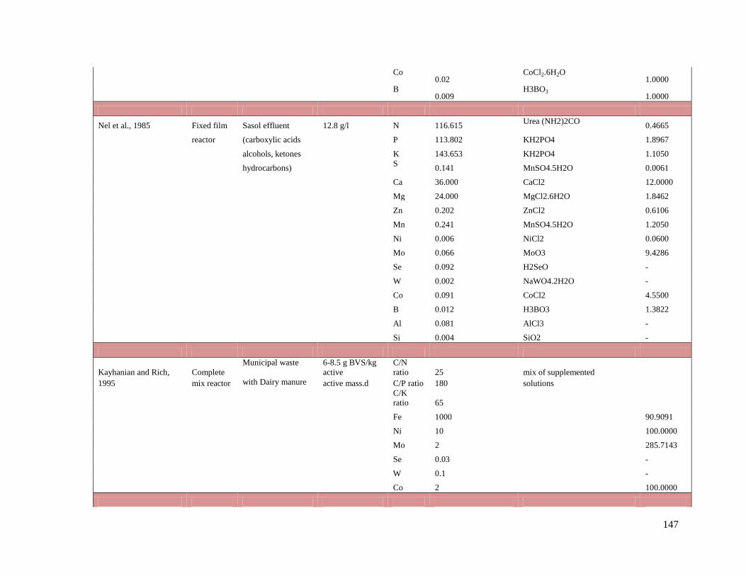
147

Co 0.02

CoCl2.6H2O 1.0000

B

0.009 H3BO3

1.0000

Nel et al., 1985 Fixed film Sasol effluent 12.8 g/l N 116.615 Urea (NH2)2CO

0.4665

reactor (carboxylic acids

P 113.802 KH2PO4 1.8967

alcohols, ketones

K 143.653 KH2PO4 1.1050

hydrocarbons)

S 0.141 MnSO4.5H2O 0.0061

Ca 36.000 CaCl2 12.0000

Mg 24.000 MgCl2.6H2O 1.8462

Zn 0.202 ZnCl2 0.6106

Mn 0.241 MnSO4.5H2O 1.2050

Ni 0.006 NiCl2 0.0600

Mo 0.066 MoO3 9.4286

Se 0.092 H2SeO -

W 0.002 NaWO4.2H2O -

Co 0.091 CoCl2 4.5500

B 0.012 H3BO3 1.3822

Al 0.081 AlCl3 -

Si 0.004 SiO2 -

Kayhanian and Rich, Complete

Municipal waste 6-8.5 g BVS/kg

active

C/N

ratio 25 mix of supplemented

1995 mix reactor with Dairy manure active mass.d C/P ratio 180 solutions

C/K

ratio 65

Fe 1000

90.9091

Ni 10

100.0000

Mo 2

285.7143

Se 0.03

-

W 0.1

-

Co 2 100.0000

148

Gonzalez-Gil et al., Batch Methanol 5 g /l N 78.438 NH4Cl 0.3138

2003

P 185.843 NaHPO4,KH2PO4 3.0974

K 117.295 KH2PO4 0.9023

S 32.066 Na2S 1.3942

Ca 35.670 CaCl2 11.8899

Mg 12.153 MgCl 0.9348

Fe 0.419 FeCl2 0.0381

Cu 0.006 CuCl2 0.0424

Zn 0.033 ZnCl2 0.0991

Mn 0.027 MnCl2 0.1373

Mo 0.010 Na2MoO4.2H2O 1.3706

Se 0.008 Na2SeO3 -

W 0.018 Na2WO4 -

B 0.011 H3BO4 1.2013

Shelton and Tiedje, Batch Various 0.05 g C/l N 138.780 NH4Cl 0.5551

1984

P 123.694 K2HPO4,KH2PO4 2.0616

K 234.706 K2HPO4,KH2PO4 1.8054

S 66.752 Na2S.9H2O 2.9023

Ca 20.446 CaCl2.2H2O 6.8154

Mg 14.480 MgCl.6H2O 1.1139

Fe 5.618 FeCl2.4H2O 0.5107

Cu 0.014 CuCl2 0.0945

Zn 0.024 ZnCl2 0.0727

Mn 0.139 MnCl2.4H2O 0.6940

Ni 0.012 NiCl2.6H2O 0.1235

Mo 0.004 NaMoO4.2H2O 0.5665

Se 0.023 Na2SeO3 -

Co 0.124 CoCl2.6H2O 6.1922

B 0.009 H3BO3 0.9714

149

Patidar and Tare, UASB Sulphate laden 1.9 -5.75 g/l.d Fe 0.25-0.5 0.0455

2004 ABR organics

Zn 0.5

1.5152

HABR

Ni 0.5

5.0000

Mo 0.2

28.5714

Co 0.2-0.3 15.0000

Wood and Tchobano- - Typical inorganic Na min 1 -

glous, 1975

Growth medium

Cl min 1

-

K min 3

0.0231

Ca 3.0- 5.0

1.6667

Mg 3.0-10.0

0.7692

Fe 1.0- 4.0

0.3636

Zn 0.02- 0.05

0.1515

Mn 0.02- 0.05

0.2500

Mo 0.02- 0.05

7.1429

Co 0.02- 0.05 2.5000

150

9. Appendix B: Analytical Methods

9.1 ICP-AES Analysis Inductively Coupled Plasma-Atomic Emission Spectroscopy (ICP-AES) is used to determine metal

concentrations for liquid samples. The instrument works on the principle that atoms emit

electromagnetic radiation as they move from an excited state to their ground state. The radiation

emitted can be detected easily when it is in a vacuum ultraviolet, ultraviolet, visible or infrared

region. There are three general steps involved and these are atom formation, excitation and

emission. ICP-AES uses plasma for the atomization and excitation steps (Manning and Grow,

1997).

The analytical method involves sample preparation, standard solutions preparation, instrument

calibration and sample analysis. Quality control is also required during sample analysis to ensure

the validity of the results obtained.

9.1.1 Sample Preparation

ICP-AES analysis may only be performed on liquid samples that do not contain solid particles.

Sample preparation thus involved filtration using a 0.45 µm pore sized filter paper. Removal of fine

solid particles prevents the nebulizer and thin tubing of the instrument from getting blocked. If

samples were not analysed immediately, they were kept refrigerated at -4°C. This prevents changes

in the concentration of ions within the samples.

9.1.2 Standard Solutions preparation

The standards used to calibrate the machine were prepared a day in advance and refrigerated

overnight. The standard solutions are required to calibrate the instrument’s response with respect to

the concentration of metal. Compounds containing the elements were used together with distilled

water for the standard solutions so that standards containing elements of known concentration were

prepared. 200 ppm stock solutions for each element were prepared and used for the standard

solution preparation. Elements were put together in groups in such a way that interferences were

not present during analysis. The following table shows the compounds used to prepare the

standards solutions and the concentrations used for calibration according to the concentrations

expected from the samples during analysis.

151

Table A2: Standard Solutions used for ICP-AES calibration

Compound Used Element 0.01 ppm 0.05 ppm 5 ppm 10 ppm 20 ppm 50 ppm

GROUP I

H3BO3 B 0.01012 0.05060 5.05986 10.11972 20.23944 50.59859

CuCl2.2H2O Cu 0.00978 0.04890 4.88955 9.77910 19.55820 48.89550

MnCl2.4H2O Mn 0.01008 0.05041 5.04105 10.08210 20.16420 50.41049

CaCO3 Ca 0.00980 0.04900 4.90026 9.80052 19.60103 49.00258

C4H4KO7Sb Sb 0.00960 0.04802 4.80198 9.60395 19.20791 48.01977

GROUP II

KCl K 0.01003 0.05016 5.01644 10.03287 20.06574 50.16435

NaCl Na 0.00969 0.04847 4.84732 9.69464 19.38927 48.47318

LiCl Li 0.00999 0.04996 4.99610 9.99220 19.98440 49.96099

(NH4)6Mo7O2.4H2O Mo 0.00960 0.04801 4.80104 9.60207 19.20415 48.01037

GROUP III

CoCl2.6H2O Co 0.00997 0.04987 4.98723 9.97447 19.94893 49.87234

Na2HPO4 P 0.00975 0.04875 4.87487 9.74974 19.49948 48.74870

GROUP IV

Al2 (SO4)3.18H2O Al 0.00975 0.04877 4.87695 9.75389 19.50778 48.76945

ZnCl2 Zn 0.00988 0.04938 4.93846 9.87692 19.75384 49.38459

K2Cr2O7 Cr 0.00977 0.04884 4.88438 9.76877 19.53753 48.84383

HgSO4 Hg 0.00910 0.04551 4.55064 9.10128 18.20256 45.50639

GROUP V

FeCl3.6H2O Fe 0.00995 0.04977 4.97663 9.95326 19.90652 49.76629

MgCl2.6H2O Mg 0.00963 0.04816 4.81639 9.63277 19.26554 48.16386

NiCl2.6H2O Ni 0.01000 0.05000 4.99973 9.99947 19.99893 49.99733

The distilled water used in preparing the standards was used as the reagent blank for analysis.

Therefore, any metal concentrations found in the reagent blank were subtracted from the standards.

Element concentrations were determined on one or two wavelengths whereby not more than one

element was determined per wavelength.

9.1.3 Quality Control

Due to the nature of the ICP-AES analysis, a quality check is necessary. Standard solutions were

used as a check between analysing of samples. The resultant concentrations were then compared to

the actual concentrations of the solutions. As another measure, samples were analysed in triplicate

and the average value was used.

152

9.2 Acid Digestion of Sludge In order to evaluate the amount of metals within solid samples such as soil and sludge, the sample

is required to undergo acid digestion to extract all the metals from the solid into a liquid phase. The

resultant liquid sample is then filtered, as mentioned in the ICP-AES sample preparation, before

undergoing ICP-AES analysis. Acid digestion extracts metals out of the solid phase through the

addition of reagents such as acids or oxidizing agents while heating the sample using a microwave

digester or hot plate. Both microwave digestion and the hot plate refluxing are presented in Martin

et al (1998). Since the hot plate refluxing method was used, the details regarding the method and

reagents are explained.

9.2.1 Apparatus and Reagents

150 ml glass beaker (digestion vessel)

Watch glass (vapour recovery device)

Hot plate (At temperature of 95°C)

Nitric acid (Concentrated)

Hydrochloric acid (Concentrated)

Hydrogen peroxide (30%)

100 ml volumetric flask

9.2.2 Method

Prior to execution of any experiment, ensure all glassware has been soaked for 48 hours in

dilute hydrochloric acid.

Mark a 5 ml level on the digestion vessel.

Measure a 1-2 g sludge sample in a digestion vessel. Do this three times for triplicate

samples which will undergo the digestion. The final metal concentration will be the average

concentration of the three samples.

Use three empty digestion vessels for three blank samples.

Add 10 ml of nitric acid (1:1 with distilled water).

Place on the hot place and cover with the watch glass.

Heat the sample to 95°C ± 5°Cand reflux for 10- 15 minutes without boiling.

Remove from the hot plate and allow the sample to cool.

Add 5 ml concentrated nitric acid, cover with the watch glass and reflux for 30 minutes.

If brown fumes are generated, oxidation is still taking place and the previous step should be

repeated until no brown fumes are observed.

153

Leave the vessel on the hot plate until the liquid reaches a volume of approximately 5 ml.

Remove the vessel from the hot plate and allow the sample to cool.

Add 2 ml of water and 3 ml of 30% hydrogen peroxide cover with the watch glass and

return to the hot plate. Care should be taken that losses do not occur due to vigorous

effervescence.

Reflux until the effervescence subsides.

Add 1 ml of 30% hydrogen peroxide and reflux.

Repeat the previous step until the effervescence is minimal and the sample appears to be

relatively unchanged.

Leave the vessel on the hot plate until the liquid within the vessel reaches a volume of

approximately 5 ml.

Remove from the hot plate and allow the sample to cool.

Add 10 ml of concentrated hydrochloric acid, cover the vessel with the watch glass and

reflux for 15 minutes.

Remove the vessel from the hot plate and allow the sample to cool.

Pour the sample into the volumetric flask and dilute to 100 ml.

Filter the liquid using 0.45 µm pore sized filter paper in preparation for ICP-AES analysis.

After ICP-AES analysis has been performed, subtract the amount of metals found within

the blanks from the amount found within the samples.

9.2.3 Obtaining the sludge samples for acid digestion

For Experiment A, the following was performed to obtain the sludge samples for acid digestion:

The residual volume, which was the volume in the reactor that contained the settled sludge

(approximately 3.5l) after decanting the supernatant, was used to represent the amount of

wet sludge in the reactor.

This wet sludge was mixed for 5 minutes using the magnetic stirrer.

Since it was found that the magnetic stirrer was not always effective for mixing the sludge,

approximately 10ml of the wet sludge was obtained at three different depths of the residual

volume. Therefore, the total amount of sludge extracted for sampling purposes was

approximately 30ml.

From the 30ml of sludge collected, 3 samples, between 1-2g were obtained using a wide

mouth automatic pipette. The mass of the sample was determined using a scale and

thereafter the sample was subjected to acid digestion.

154

For Experiment B, the following was performed to obtain the sludge samples for acid digestion:

The residual volume, which is the volume left in the reactor after decanting (7.5l for

Experiment B) only contained approximately 3.5l of sludge since this was the volume of

sludge that the reactor was seeded with at the start of the experiment. Therefore, the

residual volume was not mixed prior to sampling for sludge.

To remove any remaining supernatant in the pipes from decanting, the peristaltic pump was

used to pump the sludge from the bottom of the reactor to the top of the reactor to displace

any remaining effluent.

A sludge sample of approximately 10ml was obtained. From this sludge sample, 3 samples,

between 1-2g were obtained using a wide mouth automatic pipette. The mass of the sample

was determined using a scale and thereafter the sample was subjected to acid digestion.

9.2.4 Calculating the total amount of metals in the reactor

For Experiment A, the acid digestion was used to calculate the total amount of metals in the sludge

at the start and at the end of a cycle as well as the amount of metals in the supernatant for the mass

balance. Since the reactor feed did not contain any solids, acid digestion was not required and ICP-

AES analysis was directly performed.

The total amount of each metal in the sludge was calculated as follows:

Mass of sample (g) Volume of Sample(ml)

Sample 1 1.02 1

Sample 2 1.16 1

Sample 3 1.12 1

Average 1.1 1

Density of sludge (kg/l) 1.1 (average mass of samples / average volume of samples)

Volume of sludge (l) 3.58

(calculated using the inner diameter of the reactor and height of the

sludge)

Mass of sludge (kg) 3.938 (volume of sludge x density of sludge)

Average ICP concentration of blank samples (mg/l) 0.32

Sample 1 Sample 2 Sample 3

ICP concentration (mg/l) 4.13 3.75 4.21

Concentration (mg/l) = 4.13-0.32 = 3.81 = 3.75-0.32 = 3.43 = 4.21-0.32 = 3.89

Concentration (mg/kg)

=3.81 x 0.1 x1000/1.02

= 373.5

=3.43 x 0.1 x1000/1.16

= 295.7

=3.89 x 0.1 x1000/1.12

= 347.3

155

Average concentration

(mg/kg) 338.8

(the 0.1 above is the final volume of the sample

after acid digestion has been complete)

Metal in sludge (mg) =338.8 x 3.938 = 1334.3

The total amount of each metal in the supernatant was calculated as follows:

Mass of sample (g) Volume of Sample(ml)

Sample 1 1.52 1.5

Sample 2 1.56 1.5

Sample 3 1.53 1.5

Average 1.54 1.5

Density of effluent (kg/l) 1.02 (average mass of samples / average volume of samples)

Volume of effluent (l) 1

Mass of effluent (kg) 1.02 (volume of effluent x density of effluent)

Average ICP concentration of blank samples (mg/l) 0.12

Sample 1 Sample 2 Sample 3

ICP concentration (mg/l) 1.13 1.35 1.21

Concentration (mg/l) = 1.13-0.12 = 1.01 = 1.35-0.12 = 1.23 = 1.21-0.12 = 1.09

Concentration (mg/kg)

=1.01 x 0.1x1000 /1.52

= 66.4

=1.23 x 0.1 x1000/1.56

=78.8

=1.09 x 0.1 x1000/1.53

= 71.2

Average concentration

(mg/kg) 72.1

(the 0.1 above is the final volume of the sample

after acid digestion has been complete)

Metal in sludge (mg) =72.1 x 1.02 = 73.5

9.3 Sequential Extraction The sequential extraction procedure provides insight into the different phases the metals occur in

within a sludge sample. The procedure recommended by Stover et al, (1976) was used. Reagents

KNO3, KF, Na4P2O7, EDTA and HNO3 were used to sequentially extract metals in the

exchangeable, adsorbed, organically bound, carbonate precipitate and sulfide precipitate forms

respectively.

9.3.1 Apparatus and Reagents

Shaking table

100 ml conical flasks that securely fit onto the shaking table.

Centrifuge

KNO3 (1 M)

KF (0.5 M)

156

Na4P2O7 (0.1 M)

EDTA (0.1 M)

HNO3 (1M)

HCl (concentrated)

Furnace (550°C)

Volumetric flasks (25 ml and 50 ml)

9.3.2 Method

Prior to experimentation, soak all glassware in dilute acid for at least 48 hours.

Take a sample of sludge that has a known volume and measure the mass of the sample. The

mass of the sludge sample should be between 1 and 2 grams.

Centrifuge the samples at 5000 rpm for 10 minutes.

Remove the liquid from the solids and place in a 25 ml volumetric flask so that the sample

may be diluted up to 25 ml with distilled water.

Place the solid sample into the 100 ml conical flask. Add 30 ml of 1 M KNO3. If necessary,

rinse the centrifuge tubes with some of the reagent to try and recover all the solids.

Place samples onto the shaking table and shake for 16 hours at 20°C.

Once shaken, the liquid and solid phase of the sample needs to be separated. Centrifuge the

samples at 5000 rpm for 10 minutes. If the separation is not adequate, filtration should be

used.

Care should be taken when centrifuging and filtering as all the solids need to be recovered.

If required, use some of the reagent for the next step to recover all the solids.

Place the liquid in a 50 ml volumetric flask and dilute the sample up to the mark with

distilled water.

Place the solid sample back into the conical flask. The procedure described should be

repeated KF, Na4P2O7, EDTA and HNO3 with the following reagent volumes and shaking

settings:

157

Table 20: Reagent Scheme for the sequential extraction procedure


Exchangeable 30 ml, 1 M, KNO3 20°C, shake for 16 hours

Adsorbed 48 ml, 0.5 M, KF 20°C, shake for 16 hours

Organically Bound 48 ml, 0.1 M, Na4P2O7 20°C, shake for 16 hours

Bound to Carbonates 48 ml, 0.1 M, EDTA 20°C, 2X 8 hour shake

Bound to Sulphides 30 ml, 1 M, HNO3 20°C, shake for 16 hours

Following the last reagent addition and shaking time, separate the liquid from the solids by

filtration.

Place the filter paper with solids in a dry crucible and place in a furnace at 550°C for 1.5

hours.

Allow the filter papers with samples to cool in a desiccated environment.

Take the filter papers and add 30 ml of HCl to the ash and allow to soak before filtering the

HCl through the ash. Place the HCl in a 50 ml volumetric flask and dilute the sample to the

mark.

All samples should be filtered through a 0.45µm filter paper before undergoing ICP-AES

analysis.

If samples need to be stored before ICP-AES analysis, storage should be done at 4°C.

The concentration determined from the ICP-AES analysis should be converted to

mass/mass of sample units (mg/kg sample) by using the mass of sample and the final

volume of the diluted sample.

158

10. Appendix C: Initial Conditions for Mass Balance-Speciation

Modelling

The initial conditions for the mass balance-speciation modelling were found using a dynamic

physio-chemical model that was developed using WEST (Van Zyl et al 2012). Values from the

model were added to reactor feed concentrations and the subsequent values were used as an input

into VM. Although the system in WEST was a continuous membrane reactor, it was still used to

provide initial conditions for the reactors. Appropriate reactor volumes and feed concentrations

were used according to the setup. The following tables provide the initial conditions found for both

the reactors for Experiment A and B:

Table 21: Initial Concentrations used in VM for Experiment A, Reactors I and II

Initial Concentration (mol/l)

Species Reactor I Reactor II

Na+ 3.498E-02 4.483E-02

H+ 4.710E-02 4.433E-02

CO3 2- 4.956E-02 4.768E-02

NH4+ 3.218E-02 3.117E-02

PO4 3- 1.470E-03 1.471E-03

Cl- 5.584E-02 6.563E-02

K+ 1.938E-02 1.938E-02

HS- 2.313E-03 2.313E-03

Ca2+ 1.893E-03 1.893E-03

Mg2+ 9.838E-03 9.838E-03

Fe2+ 2.068E-03 2.068E-03

Cu2+ 1.760E-05 1.760E-05

Zn2+ 1.712E-05 1.712E-05

Mn2+ 1.120E-04 1.120E-04

MoO4 2- 1.171E-05 1.171E-05

Co2+ 1.401E-04 1.401E-04

H3BO3 1.024E-04 1.024E-04

Acetate 1.085E-04 1.359E-04

159

Table 22: Initial Concentrations used for Experiment B

Species Initial Concentrations (mol/l)

Na+ 3.718E-02

H+ 1.019E-01

CO3 2- 6.109E-02

NH4+ 2.411E-02

PO4 3- 7.390E-04

Cl- 2.721E-04

K+ 7.389E-04

HS- 0.000E+00

Ca2+ 1.663E-05

Mg2+ 1.189E-04

Fe2+ 4.377E-05

Cu2+ 5.246E-07

Zn2+ 1.121E-06

Mn2+ 8.090E-07

MoO4 2- 1.621E-08

Co2+ 7.541E-08

H3BO3 1.850E-07

SO4 2- 2.056E-04

Ni2+ 3.786E-07

I- 5.684E-09

Acetate 2.247E-02

Butyrate 5.199E-03

Propionate 9.272E-03

Valerate 2.304E-03

160

11. Appendix D: Illustration of the Mass balance in the Mass

balance-Speciation model

The mass balance portion of the model was performed using Excel. The mass balance for both

Experiment A and B accounted for the addition of metals into the system via the feed as well as the

loss of metals via the supernatant (and a small amount of sludge that is in the supernatant) that was

decanted at the end of each cycle. During the cycle, the amount of sludge in the reactor will

increase due to the growth of the microorganisms. For this research, it is assumed that the amount

of sludge that is lost via the supernatant is equivalent to the amount of sludge that increased due to

the growth of the microorganisms.

11.1 Mass balance for Experiment A Reactor volume = 6.5 l

Volume of the initial sludge = 3.5 l

Volume of sludge before decanting = volume of initial sludge + volume of sludge growth

=3.5 l + 0.01 l = 3.51 l

Working volume = volume of sludge before decanting + volume of feed

= 3.51 l + 1l = 4.51 l

Residual volume (volume after decanting) = working volume – volume of supernatant decanted –

Volume of sludge lost in decant

= 4.51 l – 1l – 0.01 l = 3.5 l

The mass balance performed in the model for Experiment A was performed as follows:

(

) ( )

(

) ( )

(

) ( )

(

) ( )

11.2 Mass balance for Experiment B Reactor volume = 9 l

Volume of the initial sludge = 3.5 l

161

Volume of sludge before decanting = volume of initial sludge + volume of sludge growth

=3.5 l + 0.01 l = 3.51 l

Volume of the supernatant before decanting = 5 l

Working volume = volume of sludge before decanting + volume of supernatant before decanting

= 3.51 l + 5l = 8.51 l

Residual volume (volume after decanting) = working volume – volume of supernatant decanted –

Volume of sludge lost in decant

= 8.51 l – 1l – 0.01 l = 7.5 l

The mass balance performed in the model for Experiment B was performed as follows:

(

) ( )

(

) ( )

(

) ( )

(

) ( )

162

12. Appendix E: Mass balance-Speciation Modelling for

Experiment A, Reactor II.

A combination of Visual Minteq (VM) and Microsoft Excel was used for the mass balance-

speciation modelling. For each cycle, the effect of decanting and feeding, as well as growth were

accounted for using mass balances in Excel. VM was used to determine the chemical speciation of

the system at the end of each cycle just before decanting. Results from VM were used as an input to

the mass balances in Excel and once decanting, feeding and growth were accounted for, resultant

values were used as an input to VM. This process was performed until the system reached pseudo-

equilibrium with respect to ion concentrations. The number of cycles modelled does not represent

experimental cycles, but is the number required until the ion concentrations at the end of each

modelled cycle are approximately constant.

12.1.1 Soluble Concentration Changes

The figure that follows displays the model prediction of concentration of ions in the dissolved

phase for K, Mg, Ca and Fe, and how they change with each successive cycle modelled.

Figure 34: : Concentration of ions in the dissolved phase for Ca, Fe, K and Mg ions, and their changes with each

successive cycle modelled for Reactor II, including comparisons to experimental values for Fe and Mg (mg/l).

The model predicted graphs represent a number of points where each point represents one cycle

modelled. At a glance, the system reaches a pseudo-steady state whereby the species reach a

0.0

0.5

1.0

1.5

2.0

2.5

3.0

3.5

4.0

0 5 10 15 20 25

Solu

ble

ion

co

nce

ntr

atio

n (

mg/

l)

Cycle

Fe2+ Exp Mg2+ Exp K+ Mg2+ Ca2+ Fe2+

163

constant concentration. For all the ions, the concentrations are predicted to increase from the initial

point until they plateau. This is due to the selected hypothetical initial concentrations being lower

when compared to the concentration that the species tend to. As a function of the model

assumptions, the species concentrations should tend to the concentration that is added via the feed

for each cycle if that species is not being precipitated. This is observed for the potassium,

magnesium and calcium ions where the model feed concentrations were 3.41, 1.08 and 0.34 mg/l

respectively, matching the final predicted supernatant concentrations. For iron, the feed

concentration was 0.52 mg/l but when compared to the final modelled dissolved concentration 0.25

mg/l, it would indicate that the model predicts that this metal is being precipitated.

With regards to the comparison between the predicted and experimentally determined values, the

experimentally determined values for both iron and magnesium are generally higher than the model

predictions. The largest discrepancy exists with magnesium where the experimental values are

approximately three times higher than the model predicted values. Since most of the experimentally

determined values are higher, it suggests the possibility that there are other processes or mass

transfer effects that may be involved.

The figure that follows displays the predicted dissolved ion concentrations for species in the µg/l

range, and their changes with modelling each successive cycle. The graph also displays the

comparison between the predicted value and the concentration determined experimentally for

copper and zinc.

164

Figure 35: Concentration of ions in the dissolved phase for Mn, Cu and Zn ions (µg/l), and their changes with each

successive cycle modelled for Reactor II, including comparisons to experimental values for Cu and Zn.

While most ions have reached a level dissolved concentration, the manganese ion displays a trend

that is increasing continually at an increasing rate. This trend suggests that manganese, which has a

feed concentration of 28 µg/l, was initially predicted to precipitate but then started to dissolute into

the soluble phase in the latter cycles, causing the predicted soluble concentration to increase. If no

further precipitation is predicted as more cycles are modelled, the soluble concentration would

increase and tend towards the feed concentration of 28 µg/l.

The feed concentration for both copper and zinc was 5 µg/l. Since the final model predicted values

were significantly lower for both copper (0 µg/l) and zinc (0.73 µg/l) the model suggests that all of

the copper ions and most of the zinc ions will be sequestered in precipitates. This is somewhat

reflected in the experimental analysis where both zinc and copper were not found in the soluble

phase (figures 11 and 12 respectively). Although the model predicts that some zinc will occur in the

soluble phase, the discrepancy between the model predicted and experimentally determined values

could be attributed to the difficulty and limitations associated with determining metal

concentrations in the micro ranges experimentally.

0.0

1.0

2.0

3.0

4.0

5.0

6.0

7.0

8.0

0 5 10 15 20 25

Co

nce

ntr

atio

n (

ug/

l)

Cycle

Cu2+ Mn2+ Zn2+ Cu2+ Exp Zn2+ Exp

165

The graph that follows displays the dissolved ion concentrations for ionic species Co2+

and HS-1

, in

the μg/l range, as well as their changes with modelling each successive cycle.

Figure 36: Concentration of ions in the dissolved phase for Co2+ and HS-1 (μg/l), and their changes with each

successive cycle modelled for Reactor II.

The two ions above are predicted to occur in minute concentrations. The model predicts that these

ions reach concentrations of about 0.08 and 0.15 μg/l for the cobalt and hydrogen sulphide ions

respectively. Although sulphur is regarded as a macronutrient, since it is required by

microorganisms and dosed into the system in macro concentrations, it is found in the soluble micro

concentration range (µg/l range). This suggests that bulk of the sulphur lies in one of the other

metal phases. For cobalt, the feed concentration was 37 µg/l, and it was not detected

experimentally, possibly because the concentration in the soluble phase was below the detection

limit. This suggests that, like hydrogen sulphide, a significant portion of this ion is predicted to

occur in phases other than the soluble phase.

12.1.2 Precipitate Formation

The model predicts the formation of a number of possible precipitates. From this list, precipitates

most likely to occur under reactor conditions were allowed to precipitate. A key result from this

was the percentage of a metal ion that was found within precipitates. The following graph displays

the changes in the amount of ion within precipitates with each cycle modelled.

0.00

0.05

0.10

0.15

0.20

0.25

0.30

0 5 10 15 20 25

Co

nce

ntr

atio

n (μ

g/l)

Cycle

Co2+ HS-1

166

Figure 37: Percentage of ions that are within precipitates as predicted for each successive cycle modelled.

A significant result from the graph above is that the model predicts that certain metals occur

completely within precipitates from the start of the experiment. These metals include Co2+

, Cu2+

and also the anion HS- (not measured experimentally). This suggests the possibility that these

metals may never occur in a bioavailable phase for micronutrient absorption. Mn2+

is initially

predicted to occur mostly within precipitates, however, as conditions change with each cycle

modelled, the amount found within precipitates decreases. This was reflected in figure 15 where an

increase in the Mn2+

soluble concentration was observed through the cycles. A similar trend for

Zn2+

and Fe2+

are observed where the amount of ion predicted to occur within precipitates are

initially higher and then decrease through the cycles as conditions within the reactor change. For

Mg2+

, K+ and Ca

2+, the model predicts that these metals occur within the soluble phase only.

Since the experimental values representing precipitates are taken as the total ions from the acid

digestion minus the soluble ions from the supernatant analysis, it is anticipated that the amount of

precipitates will be over-represented. When comparing the predicted values to the experimentally

determined values, a large discrepancy exists and part of this is due to the over-representation of

0

20

40

60

80

100

120

0 5 10 15 20 25

% o

f io

n in

pre

cip

itat

es

Cycle Ca2+ Co2+ Cu2+ Fe2+ HS-1

K+ Mg2+ Mn2+ Zn2+ Mg2+ Exp

Fe2+ Exp Zn2+ Exp Cu2+ Exp

Co2+

, Cu2+

, HS-

Mg2+

, Ca2+

, K+

Fe2+

Zn 2+

Mn 2+

167

precipitates for the experimental values. With the exception of Cu2+

which compares well to the

model predicted value, the experimental values for the rest of the ions are higher than the model

predicted values.

168

13. Appendix F: Experiment B results for Reactor I

The experimental results for reactor I were obtained and processed in an identical manner to reactor

II.

13.1 Results Summary The table below summarizes the results obtained for reactor I where negative cycles represent

cycles with micronutrient supplementation and cycle 0 represents the first cycle of operation with

the omission of micronutrient supplementation.

Table 23: Summary of experimental results for cycles -3 to 15 for Reactor I.

Cycle

Total

Biogas

Produced

(l)

%

Methane

Recovery

Max

estimated

methane

Composition

Max

estimated

CO2

composition

Max Methane

production

rate

(gCOD/min)

Minimum

pH

Time for

recovery to pH

7 (hours)

Alkalinity

dosed (g

NaHCO3)

-3 11.323 120.854 0.725 0.555 0.140 6.71 3.275 5

-2 11.842 125.461 0.722 0.577 0.138 7.2 0.000 5

-1 10.893 115.443 0.720 0.795 0.116 6.68 3.333 5

0 8.993 95.282 0.722 0.783 0.132 6.67 1.100 5

1 9.774 105.021 0.728 0.765 0.102 6.62 3.650 5

2*

5

3 6.526 61.451 0.640 0.720 0.049 6.74 10.358 5

4*

5

5 8.536 91.741 0.733 0.671 0.090 6.69 6.533 5.5

6 10.650 113.651 0.724 0.675 0.113 6.71 4.992 6

7 6.402 67.389 0.709 0.663 0.025 7.35 0.000 6.5

8 11.293 119.706 0.720 0.600 0.123 6.83 0.358 6.5

9 9.263 102.278 0.753 0.607 0.123 6.76 5.950 6.5

10 9.412 103.922 0.750 0.609 0.127 6.78 5.192 7

11 7.085 74.063 0.710 0.592 0.090 6.71 6.367 7.5

12 6.511 68.997 0.721 0.580 0.095 6.87 4.425 8

13 7.074 76.549 0.735 0.550 0.087 6.81 3.242 8

14 6.280 68.409 0.740 0.473 0.069 6.94 0.383 8

15 7.366 80.759 0.746 0.426 0.076 6.94 0.683 8

* Missing data due to power failure

13.2 Biogas Production, methane activity and methane recovery The following graph presents the total biogas production, maximum methane activity and the %

methane recovery for cycles -3 to 15 for Reactor I. The % methane recovery was calculated by

finding the total methane production in gram COD as a fraction of the feed COD.

169

Figure 38: The Total biogas production and % methane recovery on the left axis and maximum methane activity

for pre-metal washout cycles -3 to -1 and post-metal washout cycles 0 to 15 on the right axis for Reactor I.

The graph is divided into four regions using purple vertical lines. This has been performed to aid

the data interpretation for the graph. For the sake of comparison only, the total biogas produced was

multiplied by 10. Although the three variables correlate well, there is no definitive general trend

observed from the figure above. However, if the graph is observed in the four regions as shown by

the purple lines, the variables initially are unchanging until cycle 2 which corresponds to three

cycles with no micro-metals added. From cycle 2 to cycle 5, a decreasing trend is observed. The

third region, from cycle 5 to cycle 10, seems to be a recovery period where after an initial dip, the

variables increase and stabilize. From cycle 10 onwards the variables have decreased by about one

third of the values observed before the micronutrient washout.

13.3 pH Control For the cycle’s pre-metal washout, a dosage of 5 g NaHCO3 was administered. It was noticed that

during the washout experiment, as the cycles progressed, a higher dosage of alkalinity was required

to stabilise the pH to a value above 7. If the time taken for a reactor to reach a pH of 7 after the

feeding stage was greater than four hours, then the dosage for the next cycle was increased by 0.5 g

NaHCO3. The graph that follows shows the time taken for the reactor to recover the pH and the

amount of alkalinity dosed for each cycle.

0.000

0.020

0.040

0.060

0.080

0.100

0.120

0.140

0.160

0

20

40

60

80

100

120

140

-5 0 5 10 15 20

Max

me

than

e r

ate

(gC

OD

/min

)

Tota

l Bio

gas

Pro

du

ced

(lit

res)

%

Me

than

e R

eco

very

Cycle

Total Biogas Produced (*10¯ˡ litres) % Methane Recovery

170

Figure 39: Time required to reach pH recovery and the subsequent increment in dosage for the following cycle for

Reactor I.

From the graph above, it may be seen that for cycles 3, 5, 6, 9, 10, 11, and 12, the pH recovery

times are all greater than four hours, thus, a 0.5 increment in dosage was applied to the subsequent

cycles. When the graph is divided into the four regions, in the first region, stable operation is

observed while in the second, the dosage was increased due to a long time required for pH

recovery. In the third region, a fluctuating trend is observed while in the last region, an increase in

dosage results in a decrease in the recovery time.

13.4 Biogas production comparison to alkalinity dosage In the graph that follows, the alkalinity dosage and the total biogas production are compared

together with the maximum estimated CO2 composition.

0

2

4

6

8

10

12

-4 -2 0 2 4 6 8 10 12 14 16

Tim

e f

or

reco

very

(h

ou

rs)

Alk

alin

ity

do

sed

(g

NaH

CO

3)

Cycle

Time for recovery to pH 7 (hours) Alkalinity dosed (g NaHCO3)

171

Figure 40: Comparison between Total biogas produced and alkalinity dosed for cycles -3 to 15, Reactor I.

The maximum estimated CO2 composition has a similar trend to that of the total biogas produced,

except for cycle -3 and -2. In cycle -3 and -2, the total biogas production is still high but this is

more due to methane production than CO2 production. In the first region, the alkalinity dosage

remains the same however the total biogas production decreases. In the second region, the alkalinity

dosage is increased once. In the third region, the alkalinity dosage increases thrice, and this seems

to have a positive effect on the biogas production. In the fourth region, this trend does not last and

although the alkalinity dosage is increased, the biogas production as well as the maximum

estimated CO2 composition decrease. This suggests that CO2 producing biological processes have

decreased in rate or ceased completely, either due to micronutrient limitation or poor pH buffering.

The varying dosage strategy used modifies the amount of alkalinity dosed to maintain some

measure of pH buffering stability. Therefore, in these cases, the effect of poor buffering is not the

dominant factor that controls digestion stability. However, this approach indicates that the onset of

severe instability and digestion failure relative to stable operation conditions cannot be clearly seen.

However, the resulting changes in gas composition and production rate can be more directly linked

to limitations to biological process rates rather than to pH buffering problems, that may also have

other causes besides micronutrient limitation.

0

2

4

6

8

10

12

14

-4 -2 0 2 4 6 8 10 12 14 16

Tota

l Bio

gas

pro

du

ced

(lit

res)

A

lkal

init

y d

ose

d (

g N

aHC

O3)

Cycle

Total Biogas Produced (l) Alkalinity dosed (g NaHCO3)

172

13.5 Supernatant Metal Analysis Metal analysis was performed using ICP-AES analysis for supernatant samples. Acid digestion was

not required as samples contained minimal solids. The following graph displays the soluble

concentrations of Al, Ca, Mg and Fe as a percentage of their maximum concentration (C/Cmax) as

well as the amount of the metal washout in the effluent as a percentage of the amount of metal in

the feed when dosed to the system. Co, Cr, Cu, Mn and Zn were not detectable within the

supernatant and therefore are not included. Al is not a micronutrient dosed to the system, thus there

is not a % metal lost as a function of metal in the feed.

Figure 41: Soluble concentrations as a percentage of the maximum concentration as well as the amount of metal

washout as a % of the feed for cycles -2, 9 and 15, Reactor I.

The overall trend for all the soluble metal concentrations is a decreasing one. The % metal lost in

the supernatant for Ca is about five times greater than the amount fed before the metal washout

experiment. For cycles 9 and 15, Ca is still lost at a rate of between 1.4 and 2.2 times the feed mass

even though during these cycles, no Ca is fed to the system. This indicates that accumulated Ca is

being rapidly depleted by dissolution of precipitates or release from some other solid phase that has

sequestered Ca. For Fe, only 13 % of what was being fed was lost via the effluent. For cycles where

no Fe was dosed, the % metal lost is slightly lower (10%) for cycle 9 and for cycle 15, only 3% is

lost. This suggests that the Fe is possibly depleted within the reactor. For Mg, the near 100% metal

lost for cycle -2 suggests that the same amount dosed to the system is the same amount lost via the

effluent. This indicates that there is no net accumulation or depletion of Mg during a cycle with

micronutrient dosing. For cycles during the washout experiment, Mg is still lost but at a decreasing

rate.

0%

20%

40%

60%

80%

100%

120%

-2 9 15

% C

/Cm

ax

Cycle

Al Ca Fe Mg

13

10

3

490

221

142

106

43

25

→% metal lost

173

13.6 Sludge Metal Analysis Selected sludge samples were collected and subjected to acid digestion before undergoing ICP-AES

analysis. The sludge metal concentrations represent phases which are potentially or non-

bioavailable such as precipitates. The graph that follows displays the sludge metal concentrations as

a percentage of the maximum concentration (% C/Cmax) for Al, Ca, Co, Cr, Cu, Fe, Mg, Mn and

Zn.

Figure 42: Sludge metal concentrations as a percentage of the maximum concentration for selected cycles for Al,

Ca, Co, Cr, Cu, Fe, Mg, Mn and Zn, Reactor I.

For all of the metals above, a fluctuating trend for the concentration of metals within the sludge is

observed. This suggests that the metal ions are well retained within the sludge, and are not easily

depleted from the phases within the sludge due to the washout experiment.

For the sludge samples, when comparing the amount of metal within the sludge to the amount that

was dosed in the feed, the percentage of metal retained is obtained. The following graph provides

the percentage of metal retained for selected cycles for Ca, Co, Cu, Fe, Mg, Mn and Zn. Al and Cr

are not included as they are not part of the micronutrient cocktail dosed to the system pre-metal

washout.

0

0.2

0.4

0.6

0.8

1

1.2

-2 9 15

% C

/Cm

ax)

Cycle


174

Figure 43: Amount of metal retained within Reactor I as a percentage of the amount dosed via the feed for selected

cycles.

Zn and Co display values of between 250 to 1050% metals retained from cycle -3 to 15, showing

great metal retention. Mg displays the lowest ability to be retained within the sludge since before

the metal washout, only 4% of the metal was found within the sludge.

1

10

100

1000

10000

-5 0 5 10 15 20

% M

eta

l Re

tain

ed

Cycle

Ca Co Cu Fe Mg Mn Zn

Analysis of nutrient requirements for the Anaerobic ...

Documents

Transcript of Analysis of nutrient requirements for the Anaerobic ...