Chapter 9

Application of Exploratory Multivariate Analysis for Network Security

Khaled Labib and V. Rao Vemuri

Department of Applied Science, University of California, One Shields Avenue,

Davis, California 95616, U.S.A. {kmlabib, rvemuri}@ucdavis.edu

Abstract There are many ways to study, analyze, visualize and detect network traffic anomalies. Some of these are quite successful. However, it is difficult to compare the results obtained from these studies and to define the merits and demerits of each method. This difficulty is exacerbated while comparing visualization methods. A primary reason for this difficulty is the heterogeneous nature of the development process of these methods, as they do not use a common framework for the development and testing. This study uses the S language for statistical computing and graphics as a unified framework for evaluating the applicability of seven exploratory multivariate analysis methods for anomaly detection and visualization. The methods are used to study, visualize and possibly detect computer network attacks. The k-means, hierarchical clustering, self-organizing maps, principal component analysis, independent component analysis, stars plots and mosaic plots are used to analyze and visualize selected network attacks from the DARPA 1998 Intrusion detection evaluation data set. Visualization techniques associated with each method provide more in-depth representation of the nature of the network traffic with each method having its unique view of the data. Some of the results obtained may be used in identifying trends in the behavioral change in the traffic characteristics. Using this unified framework, a comparison of the performance, feature, graphical representation and applicability of each method is possible.

1. Introduction The field of intrusion detection has been the focus of many researchers for more than a decade. Several successful implementations of Intrusion Detection Systems (IDS’s) have resulted from this research. Each of these implementations generally uses its own set of home-grown software tools, scripts and programs in order to construct and validate every new IDS concept and method. The steps involved in developing and testing a new IDS method include data collection, pre-processing, algorithm development, data storage and visualization. In addition, the research and development process typically spans multiple disciplines including statistics, artificial intelligence (AI), mathematics and visualization. However, there is a lack of a unified framework for developing and testing these systems. This results in difficulties in comparing the results. Moreover, the software components developed for one system are not reusable by another system that is under development due to the lack of a common framework for reusability. Another issue arises when trying to evaluate and compare visualization methods that are created through different computer programs. In order to be able to do a meaningful comparison, several tools must be setup, each having its own flavor of graphical representation. In addition, these tools may be designed to run on different platforms making it even harder to compare these graphical representations. It is also desired to graphically characterize the development of the network traffic in general and the development of attack patterns in particular. This is an area where little research has been done. Tracking behavioral changes in the characteristics of the network traffic across time can enable earlier detection of attacks. This approach of characterizing the development of network attacks is inspired by the work of Herman and Montroll [[1]] in characterizing the development of countries.

In order to address these issues, this study proposes the use of S Language to provide a unified framework for studying, developing, testing and comparing the results of various methods for the implementation of anomaly detection systems with emphasis on visualization. Seven exploratory multivariate analysis algorithms are studied namely: the k-means, hierarchical clustering, self-organizing maps, principal component analysis, independent component analysis, stars plots and mosaic plots. Using a single program, data sets can be loaded and post-processed. Then each method is applied to the data sets. The generated statistics are displayed and graphical views of data provide for an intuitive visual approach for finding relationships amongst the different data elements. A comparison of the results obtained from running the different algorithm emphasizes the fact that each method is suitable for detecting certain anomalies while others may provide a more powerful visualization of the data. The rest of the chapter is organized as follows: Section 2 provides an introduction to the problem of intrusion detection and discusses related work in intrusion detection using the methods presented in this paper. Section 3 introduces S Language and Environment. Section 4 provides an introduction to multivariate analysis methods used in this study. Section 5 describes Denial-of-Service and Network Probe attacks. Section 6 details the process of data collection and preprocessing and the creation of feature vectors. Section 7 discusses the results obtained and suggests a method of detecting intrusions using these results.

2. The Intrusion Detection Problem With the widespread use of computer networks and telecommunication devices, network security has become an important concern for the developers and users of these networks. As a result, the problem of intrusion detection has grasped the attention of both research and corporate institutions with the aim of developing and deploying effective IDS’s that are capable of protecting critical system components against intruders. Currently, three approaches have gained some degree of popularity. The first, a signature-based method [[2]], creates a database of known intrusion signatures and compares all user signatures with this database. The disadvantage of this model is its inherent inability to detect new attacks or known attacks that have significantly changed their behavior, that is, the signature. The second approach, referred to as anomaly detection, attempts to establish what the normal traffic patterns look like for a given network, and flags out any variations in traffic from this norm. Unlike signature-based detectors, anomaly detectors do not compare the traffic against any signature database; they rather attempt to identify anomalies in the traffic that suggest a possibility of an attack or intrusion that is taking place. The disadvantages of this model are high false alarm rates and the lack of ability to easily cope with normal changes in network activity. In addition, anomaly detectors can flag out abnormal behavior, but may not be able to specify the exact type of attack or its nature. The third approach, referred to as specification-based intrusion detection, relies on manually specifying program behavioral specification that is used as a basis to detect attacks. It has been proposed as a promising alternative that combines the strengths of signature-based and anomaly-based detection [[3]]. The focus of this study is on evaluating the use of exploratory multivariate analysis methods as applied to anomaly detection with emphasis on visualization. Anomaly detection is a widely used method in the field of computer security, and there are many approaches that utilize it for detecting intrusions [[4]]. Various techniques for modeling normal and anomalous data have been developed for anomaly detection. A survey of these methods can be found in [[5]]. Clustering methods have been used in many fields including statistics [[6]], machine learning [[7]] and visualization. Some studies, summarized next, attempted to use clustering methods for anomaly detection.

Portony [[8]] presents a method for clustering similar data instances together and uses distance metrics on clusters to determine an anomaly. The author makes two basic assumptions: First, data instances having the same classification should be close to each other in feature space under some reasonable metric, while instances with different classifications should be far apart. Second, the number of instances in the training set that represent normal traffic is overwhelmingly larger than the number of intrusion instances. Clusters were labeled automatically, and were later used to classify unseen network data instances. Both training and testing was done using subsets of KDD CUP 99 data [[9]]. On average, the detection rate was around 40%-55% with a 1.3% - 2.3% false positive rate. There are a number of research projects that focus on using statistical approaches for anomaly detection. Staniford-Chen et al [[10]] address the problem of tracing intruders who obscure their identity by logging through a chain of multiple machines. They use PCA to infer the best choice of thumbprinting parameters from data. They introduce thumbprints, which are short summaries of the content of a connection. Shah et al [[11]] study how fuzzy data mining concepts can cooperate in synergy to perform Distributed Intrusion Detection. They describe attacks using a semantically rich language, reason over them and subsequently classify them as instances of an attack of a specific type. They use PCA to reduce the dimensionality of the collected data. There are some studies that attempt to apply Self Organizing Maps as a tool to address network intrusion detection in general, and denial of service attack detection in particular. A system developed by Rhodes et al [[12]] uses multiple self-organizing maps for intrusion detection. They use a collection of more specialized maps to process network traffic for each layered protocol separately. They suggest that each neural network becomes a kind of a specialist, trained to recognize the normal activity of a single protocol. Another approach that differs from anomaly detection and misuse detection considers human factors to support the exploration of network traffic [[13]]. They use self-organizing maps to project the network events on a space appropriate for visualization, and achieve their exploration using a map metaphor. The use of self-organizing maps combined with stars plots as a visualization tool in this study is motivated by the work of Herman et al. The authors attempted to characterize the temporal evolution of countries by the use of labor force distribution data on a multidimensional phase plot so that the development of a country is represented by an evolutionary track of a phase point. Similar attempt is made in this study to characterize the temporal evolution of network traffic using feature vectors of network traffic data on a multidimensional plot utilizing self-organizing map and stars plots. In the above cited works a heterogeneous set of tools and software packages were used to develop and test each method leading to difficulties in comparing the results obtained and accurately assessing the method’s performance. This issue is also common in similar work in the field. Different tools generate different output formats, reports and graphics making it hard to compare their results. In addition, the preprocessing phase of data using different programs and techniques can lead to variable performance numbers amongst the different implementations which makes the process of evaluating comparative performance difficult. Using S creates a unified framework for evaluating the results and associated performance of each method. In addition, reusability of software components can become a much easier task when using a single framework. Common to the implementation of these anomaly detection approaches is a set of tasks that are performed in order to achieve the desired goal of detecting intrusions. These tasks can be summarized as follows:

Data collection and processing: For example, sniffing data off the network and processing it to extract the desired portions of packet data.

Application of detection algorithm: The desired detection algorithm or method is applied to the data previously collected.

Evaluation of results: By generating reports and using advanced visualization to assess the results obtained.

In practice, each of these tasks may be implemented using one or more software segments. Many of the current projects evaluating new IDS concepts use a variety of different programs ranging from scripts and compiled executables to third-party tools and perhaps certain portions of code from an older project. All of the above tasks can be achieved within a single framework using S.

3. The S Language and Environment The S environment is an integrated suite of software facilities for data analysis and graphical display. “The term environment is intended to characterize it as a planned and coherent system built around a language and a collection of low-level facilities, rather than the ‘package’ model of an incremental accretion of very specific, high-level, and sometimes inflexible tools” [[14]]. One of the strengths of S is that functions implementing new statistical methods can be developed on top of the low-level facilities. For example, to create a single function to perform the three basic tasks of an IDS, as described in section 2, the S code would look like: evalIDS ← function( indata ) {

pd ← procData( indata ); intrusion ← detectIntrusion( pd ); evalResult ← evalResult( intrusion );

} The top-level function evalIDS accepts one argument, indata, and calls three functions namely procData, detectIntrusion and evalResult representing the three basic tasks. Each of the three functions in turn calls other lower level functions to implement their details. Specific examples of these functions will be discussed in details in section 7.2. Using S, it is quite easy to play around with design decisions made by the original implementers in order to explore new ideas. For example, an existing library function uses linear interpolation. This behavior can be changed to reflect a non-linear model by re-writing the function. In the previous example the function detectIntrusion could be made a library function with some default algorithm to detect intrusions. This default behavior could easily be modified, by modifying the library function source, to implement variations of the default algorithm or a completely new algorithm while maintaining the same structure of the rest of the program. This flexibility is even more evident in the open-source R implementation where all the details of implementation are open for exploration. Indeed, R is used in this study to generate all results and graphics. The commercial implementation of S, called S-Plus, has an extensive Graphical User Interface (GUI), which provides menus and dialogues for many simple statistical and graphical operations. A full-featured student edition is available at no cost for students at accredited universities. The open-source R package can be downloaded directly from the project web site and is installable on many platforms including Windows and Linux. Almost all S scripts developed for S-Plus will run on R and vice versa. The main difference between S-Plus and R is that S-Plus, including the student edition, has a sophisticated GUI that is especially helpful for new users. Both S-Plus, including the student edition, and open-source R implementations provide a command-line interface for entering S commands. Once the program is started, this command line allows the user to enter S commands, create variables, call functions, draw graphs, create and manipulate data tables, and save and print results. Since S is also a full programming language in its own right, it provides for assignment statements, control structures, arithmetical expressions, array and matrix operations and calling conventions for functions, amongst other capabilities.

Some of the language features found in S are found in other scientific analysis languages like Matlab and Mathematica, but S provides for some key features that make it more applicable for use in intrusion detection research. First, S is designed to be a statistical analysis tool and thus many of the specialized statistical functions are already available in its libraries and need not be written from scratch. These functions are typically the core functions that are used to develop intrusion detection engines. On the other hand, Matlab is essentially a numerical simulation tool that is designed to do linear algebra computations and simulation. For example, implementing statistical models from Becker et al [[15]] (commonly known as the blue book models) in Matlab is a chore, whereas, it is essentially built-in S-Plus and R. Also, S’s ability to run on many platforms makes it ideal for use in intrusion detection research where the hosts under study are running a variety of operating systems and hardware. For example, R is available for over 14 different processor architectures and operating systems including the most common ones such as Linux, Windows, MAC OS and many Unix flavors. This is a key feature for distributed intrusion detection systems where detection sensor devices need to be installed on a network of hosts with different processor architectures that run different operating systems. In this case, each sensor binary executables (an R installation) can be built from sources according to the processor architecture used at each host. On the other hand Matlab is available for five different platforms, and only in binary executables form. Furthermore, S has a powerful object-oriented language structure that can implement quite complex algorithms and their variants. Finally, S-Plus student edition is free for use by students and the open-source R is free to everyone. Open-source software packages have proved to be effective for use by research institutions that can not afford costly software licenses. Several speed and feature comparisons are available which compares S-Plus and R to other data analysis packages including Matlab, being one of the most common ones. A speed comparison between these three packages and several others can be found in [[16]]. A detailed comparison of the features available in these packages including a comparison of mathematical functionality, graphical functionality, programming environment functionality, data handling, available operating systems and speed comparison can be found in [[17]]. Using S for intrusion detection enables a researcher to study and compare the results of several detection methods using a single tool. Since S runs from a command-line interface, the processes of data collection, preprocessing, conversion to S objects (such as arrays and matrices), manipulation of data using a method of choice, generating the required statistics and plotting the results can all be done using a single tool. S comes with many pre-implemented routines that can be used without being changed. These routines cover methods from exploratory multivariate analysis, including cluster analysis, factor analysis and discrete multivariate analysis to classification methods including discriminant analysis, neural networks and support vector machines to name a few. All the methods could be replaced or changed to explore newer ideas.

4. Introduction to Multivariate Analysis Methods

4.1. Exploratory Multivariate Analysis Multivariate analysis is concerned with data sets that have more than one response variable for each observational unit. The data sets can be summarized by data matrices X with n rows and p columns, the rows representing the observations, and the columns the variables. The main division in multivariate methods is between those that assume a given structure, for example, dividing the cases into groups, and those that seek to discover the structure from the evidence of the data matrix alone, also called data mining. In pattern recognition terminology the distinction is between supervised and unsupervised methods. Most of the emphasis of this chapter is on unsupervised methods with the assumption of no apriori knowledge of the structure of data.

4.2. Visualization Methods A simple way to examine multivariate data is via a pairs plot or scatterplot matrix. Pairs plots are a set of two-dimensional projections of a high dimensional point cloud. However, a pairs plot can easily miss interesting structures in the data that depend on three or more variables, and genuinely multivariate methods explore the data in a less coordinate-dependent way. Many of the visualization methods can be viewed as projection methods for particular definitions of “interestingness”. Feature vectors dimensions used in this study have p = 12 columns, therefore, several visualization techniques are applied that attempt to reduce the dimensionality of these vectors. In the following sections, a brief description of each of the methods used in this study is provided.

4.3. Clustering Methods Cluster analysis is concerned with discovering groupings among the cases of an n by p matrix, where n is the number of observations and p is the number of variables in each observation. A comprehensive general reference can be found in [[18]]. Cluster analysis searches for groups (clusters) in data in such a way that objects belonging to the same cluster resemble each other, whereas objects in different clusters are dissimilar. In two or three dimensions, clusters can be visualized; with more than three dimensions, some kind of analytical assistance and simplified visualization are necessary. Generally speaking, clustering algorithms fall into two categories [[19]]: (a) Partitioning Algorithms: A partitioning algorithm describes a method that divides the data set into k

clusters, where the integer k needs to be specified. Typically, the algorithm is run for a range of k-values. For each k, the algorithm carries out the clustering and also yields a quality index, which allows the selection of the best value of k afterwards. The S functions kmeans, pam, clara, and fanny implement algorithms of this type.

(b) Hierarchical Algorithms: A hierarchical algorithm describes a method yielding an entire hierarchy of

clustering for the given data set. Divisive methods start by considering the whole data set as one cluster, and then splits up clusters until each object is separate. Algorithms of this type are used in the S functions diana and mona. The seven functions daisy, pam, clara, fanny, agnes, diana, and mona make up the cluster library. Algorithms to implement these functions are described in [[20]].

4.3.1. Partitioning Methods

Partitioning methods are based on specifying an initial number of groups, and iteratively reallocating observations among groups until some equilibrium is attained.

4.3.1.1. k-means Clustering One of the best known partitioning methods is the k-means. In the k-means algorithm the observations are classified as belonging to one of k groups. Group membership is determined by calculating the centroid for each group (the multidimensional version of the mean) and assigning each observation to the group with the closest centroid. The k-means clustering algorithm chooses a pre-specified number of cluster centers to minimize the within-class sum of squares of the vectors for those centers. Since the algorithm needs a starting point, it chooses the mean of the clusters identified by group-average clustering. The k-means needs access to the data matrix and uses Euclidean distance. The k-means algorithm alternates between calculating the centroids based on the current group memberships, and reassigning observations to groups based on the new centroids. Centroids are calculated

using least-squares, and observations are assigned to the closest centroid based on least-squares. This use of a least-squares criterion makes k-means less resistant to outliers. The S function kmeans performs k-means clustering. It is an older function that does not have special plot or summary methods. The main arguments to kmeans are dissimilarities as produced by daisy or dist and the number of clusters. Alternatively, a matrix of starting centroids may be specified in place of the number of centroids. If starting values are not specified, the initial centroids are obtained using the hierarchical clustering algorithm in hclust.

4.3.2. Hierarchical Methods The partitioning algorithms discussed in the previous section are based on specifying an initial number of groups, and iteratively reallocating observations between groups until some equilibrium is attained. In contrast, hierarchical algorithms proceed by combining or dividing existing groups, producing a hierarchical structure displaying the order in which groups are merged or divided.

4.3.2.1. Divisive Clustering Divisive analysis starts with one group and repeatedly divides groups to form many groups. The function diana implementation, of a divisive hierarchical method, is probably unique in computing a divisive hierarchy, because most other software for hierarchical clustering is agglomerative. Moreover, diana provides (a) the divisive coefficient, which measures the amount of “clustering structure”, and (b) the banner plot. In diana, the initial clustering (at step 0) consists of one large cluster containing all n objects. In each subsequent step, the largest available cluster is split into two smaller clusters, until finally all clusters contain but a single object.

4.4. Self-Organizing Maps The Self-Organizing Map (SOM) [[21]] is a neural network model for analyzing and visualizing high dimensional data. It belongs to the category of competitive learning networks. The SOM is based on unsupervised learning to map nonlinear statistical relationships between high-dimensional input data into a two-dimensional lattice. This mapping is topology preserving. The property “topology preserving” means that points near each other in the input space are mapped to nearby map units in the SOM. SOM is a family of algorithms with no well-defined objective to be optimized, and the results can be critically dependent on the initialization and the values of the tuning constants used. Despite this high degree of arbitrariness, the method scales well and often produces useful insights in data sets whose size is way beyond, for example, Multi-dimensional Scaling (MDS) methods. If all the data is available at once, the preferred method is batch SOM. For a single iteration, assign all the data points to representatives, and then update all the representatives by replacing each by the mean of all data points assigned to that representative or one of its neighbors, possibly using a distance-weighted mean. The algorithm proceeds iteratively, shrinking the neighborhood radius to zero over a small number of iterations.

4.5. Principal Component Analysis Principal Component Analysis [[22]] is a well-established technique for dimensionality reduction and multivariate analysis. Examples of its many applications include data compression, image processing, visualization, exploratory data analysis, pattern recognition, and time series prediction. A complete discussion of PCA can be found in textbooks [[23]], [[24]]. The popularity of PCA comes from three important properties. First, it is the optimal (in terms of mean squared error) linear scheme for compressing a set of high dimensional vectors into a set of lower dimensional vectors and then reconstructing the original set. Second, the model parameters can be computed directly from the data – for example by

diagonalizing the sample covariance matrix. Third, compression and decompression are easy operations to perform given the model parameters – they require only matrix multiplication. A multi-dimensional hyper-space is often difficult to visualize. Summarizing multivariate attributes by two or three variables that can be displayed graphically with minimal loss of information is useful in knowledge discovery. Because it is hard to visualize a multi-dimensional space, PCA is mainly used to reduce the dimensionality of p multivariate attributes into two or three dimensions. PCA summarizes the variation in correlated multivariate attributes to a set of non-correlated components, each of which is a particular linear combination of the original variables. The extracted non-correlated components are called Principal Components (PC) and are estimated from the eigenvectors of the covariance matrix of the original variables. Therefore, the objective of PCA is to achieve parsimony and reduce dimensionality by extracting the smallest number components that account for most of the variation in the original multivariate data and to summarize the data with little loss of information. The S function princomp calculates the principal components of a given data matrix.

4.6. Independent Component Analysis Independent Component Analysis (ICA) has become a hot topic in data visualization. It is a method for finding underlying factors or components from multivariate (multidimensional) statistical data. What distinguishes ICA from other methods is that it looks for components that are both statistically independent, and non-gaussian. ICA looks for rotations of sphered data that have approximately independent components. This will be true (in theory) for all rotations of samples from multivariate normal distributions, so ICA is of most interest for distributions that are far from normal. The function fastICA performs independent component analysis on a given data matrix.

4.7. Stars Plots There is a wide range of ways to trigger multiple perceptions of a figure, and these can be used to represent each of a moderately large number of rows of a data matrix by an individual figure. Perhaps the best known of these is the stars plots as implemented in the function stars. This glyph plot does depend on the ordering of the variables and perhaps also their scaling, and it does rely on properties of human visual perception. So it has rightly been criticized as subject to manipulation and one should be aware of the possibility that the effect may differ by viewer. Nevertheless, it can be a very effective tool for private exploration.

4.8. Mosaic Plots Most works on visualization implicitly assume continuous measurements. However, large-scale categorical data sets are becoming more prevalent. There are some useful tools available for exploring categorical data, but it is often essential to use models to understand the data. Mosaic plots divide the plotting surface recursively according to the proportion of each factor in turn (so the order of the factors matters). For mosaic plots, the feature vectors created from the network traffic are viewed as categorical data to explore additional information in the data.

5. Denial of Service and Network Probe Attacks In a Denial-of-Service (DoS) attack, the attacker makes some computing or memory resource too busy, or too full, to handle legitimate users’ requests. But before an attacker launches an attack on a given site, the attacker typically probes the victim’s network or host by searching these networks and hosts for open ports. This is done using a sweeping process across the different hosts on a network and within a single host for services that are up by probing the open ports. This process is referred to as Probe Attacks.

Table 1 : Description of DoS and Probe Attacks

Attack Name Attack Description Smurf (DoS)

Denial of Service ICMP echo reply flood

Neptune (DoS)

SYN flood Denial of Service on one or more ports

IPsweep (Probe)

Surveillance sweep performing either a port sweep or ping on multiple host addresses

Portsweep (Probe)

Surveillance sweep through many ports to determine which services are supported on a single host

Table 1 summarizes the types of attacks used in this study. The attacks are described in more details below. Smurf attacks, also known as directed broadcast attacks, are a popular form of DoS packet floods. Smurf attacks rely on directed broadcast to create a flood of traffic for a victim. The attacker sends a ping packet to the broadcast address for some network on the Internet that will accept and respond to directed broadcast messages, known as the Smurf amplifier. These are typically mis-configured hosts that allow the translation of broadcast IP addresses to broadcast Medium Access Control (MAC) addresses. The attacker uses a spoofed source address of the victim. For Example, if there are 30 hosts connected to the Smurf amplifier, the attacker can cause 30 packets to be sent to the victim by sending a single packet to the Smurf amplifier [[25]]. Neptune attacks can make memory resources too full for a victim by sending a TCP packet requesting to initiate a TCP session. This packet is part of a three-way handshake that is needed to establish a TCP connection between two hosts. The SYN flag on this packet is set to indicate that a new connection is to be established. This packet includes a spoofed source address, such that the victim is not able to finish the handshake but had allocated an amount of system memory for this connection. After sending many of these packets, the victim eventually runs out of memory resources. IPsweep and Portsweep, as their names suggest, sweep through IP addresses and port numbers for a victim network and host respectively looking for open ports that could potentially be used later in an attack.

6. Data Collection and Preprocessing

6.1. Data Collection The 1998 DARPA Intrusion Detection data sets were used as the source of all traffic patterns in this study. The training data set includes traffic collected over a period of seven weeks and contains traces of many types of network attacks as well as normal network traffic. This data set has been widely used in intrusion detection research, and has been used in comparative evaluation of many IDSs. McHugh [[26]] presents a critical review of the design and execution of this data set. Attack traces were identified using the time stamps published on the DARPA project web site.

6.2. Data Preprocessing Data sets were preprocessed by extracting the IP packet header information to create feature vectors. The resulting feature vectors were used to calculate the principal components and other statistics. The feature vector chosen has the following format:

SIPx Sport DIPx Dport Prot Plen Where • SIPx = Source IP address nibble, where x = [1-4]. Four nibbles constitute the full source IP address. • Sport = Source Port number • DIPx = Destination IP address nibble, where x = [1-4]. Four nibbles constitute the full destination IP

address.

• Dport = Destination Port number • Prot = Protocol type: TCP, UDP or ICMP • Plen = Packet length in bytes This format represents the IP packet header information. Each feature vector has 12 components corresponding to the p columns in section 4. The IP source and destination addresses are broken down to their network and host addresses to enable the analysis of all types of network addresses. Seven data sets were created, each containing 300 feature vectors as described above. Four data sets represented the four different attack types, one for each shown in Table 1. The three remaining data sets represent different portions of normal network traffic across different weeks of the DARPA Data Sets. This allows for variations of normal traffic to be accounted for in the experiment. One of the motives in creating small data sets (i.e. 300 feature vectors each) for representing the feature vectors is to study the effectiveness of this method for real-time applications. Real-time processing of network traffic mandates the creation of small sized databases that are dynamically created from real-time traffic presented at the network interface. Since DARPA data is only available statically, seven small data sets were created to mimic the case of dynamic real-time operation. With each packet header being represented by a 12 dimensional feature vector, it is difficult to view this high-dimensional vector graphically and be able to extract the relationships between its various features. It is equally difficult to extract the relationship between the many vectors in a set. Therefore, the goal of using the several methods in this study is to reduce the dimensionality of the feature vector using various techniques. It is also important to be able to graphically show the distinctions between normal and attack traffic for each data set.

7. Results The seven multivariate analysis methods described in section 4 were applied to the data sets described in section 6. The objective is to evaluate the ability of each method to separate the first 300 feature vectors (containing normal traffic) from the next 300 feature vectors (containing attack traffic) into a different cluster. If the method can isolate all attack feature vectors into one or more clusters consistently, then its graphical representation is compared to other methods in terms of overall visual detection ability and computational performance. The goal is to do all these steps within S. Using S, the three common tasks discussed in section 2 are performed as follows:

7.1. Data Collection and Processing The following code snippet shows how the feature vector data sets are loaded into R, and how the different calls to the methods are made. Library(cluster) library(MASS) library(class) library(fastICA) ## Load Regular data frames regular1 <- read.table(“regular300.txt”, row.names=NULL) ## Load Attack data frames smurf <- read.table(“smurf300.txt”, row.names=NULL) ipsweep <- read.table(“ipsweep300.txt”, row.names=NULL) portsweep <- read.table(“portsweep300.txt”, row.names=NULL) neptune <- read.table(“neptune300.txt”, row.names=NULL)

The first four lines load pre-installed R libraries namely: Cluster library, MASS library which contains many data sets and a number of S functions, classification library and a fast ICA library. Next, data frames are created, by reading their corresponding files from disk. The data frames are named by their type. A data frame is an S object normally used to store a data matrix.

7.2. Application of Multivariate Analysis Algorithms

7.2.1. k-means Clustering k-means clustering is applied to each data set of the different attack types after binding (combining) each of their data frames with the normal traffic data in regular1 to form a new data frame called “master” with 600 rows and 12 columns. This binding process is used for the remaining data sets as well: for (dataset in masterlist){ master <- rbind (regular1, dataset) kmeansout <- kmeans(master[1:12], 2) plot(kmeansout$cluster, type = “b”, main=masterlistnames[counter] , xlab=”Packet Number”, ylab=”Cluster Number”) } The function kmeans performs k-means clustering on the combined data frame. Two arguments are given to kmeans. First, is the “master” data frame, which is the result of binding the attack dataset to the regular dataset. Second, is the number of clusters required. In this case, kmeans will attempt to cluster the 600 feature vectors, given as its input, into two clusters without any other prior knowledge of the nature of the data. The results of kmeans are then plotted using the “plot” function. The resulting four plots are shown in Figure 1. The function plots the assignment of each input vector to an output cluster. This information is stored in the kmeansout$cluster variable. Since the number of desired output clusters is two, each input feature vector is assigned to either cluster one or two as shown in the figure. A line connects the output points on the graph to provide visual continuity. In the case of Smurf, all the attack feature vectors (301 to 600) were assigned to cluster two, while all normal feature vectors (0 to 300) were assigned to clusters one and two. Similar results can be seen for IPsweep, Portsweep and Neptune data sets. For these sets, some of the attack vectors were clustered in a different cluster than the majority of the packets. Careful study of these packets shows that few normal instances of traffic existed in the midst of the attack.

Figure 1: k-means clustering plot

By increasing the number of output clusters to four, some attacks were exclusively clustered in one cluster where no normal instances were assigned, thereby, giving better clustering results than using two clusters.

7.2.2. Hierarchical Clustering Hierarchical clustering is applied to the data sets as follows: for (dataset in masterlist){ master <- rbind (regular1, dataset) hclustout <- hclust(dist(master[1:12])) plot(hclustout, main=masterlistnames[counter],xlab=”PacketNumber”) } The hclust function performs hierarchical clustering on the combined data sets. Prior to starting the hierarchical clustering process, the function dist is called to compute the distance matrix for the “master” data set. The distance matrix is computed by using a specified distance measure, in this case Euclidean, to compute the distances between the rows of the data matrix. The output “hclustout” is plotted using the plot function and is shown in Figure 2.

Figure 2: Hierarchical Clustering Plot

Figure 2 shows the dendrograms created by the hclust function. A dendrogram is a convenient method used to visualize the clustering results. It is a tree graph that is used to examine how clusters are formed in hierarchical cluster analysis. The vertical axis indicates a distance or dissimilarity measure. The height of a node represents the distance of the two clusters that the node joins. The larger the height, the more dissimilar the two clusters are. The horizontal axis lists all the 600 observations and their cluster assignments. Dendrograms have two limitations: First, because each observation must be displayed as a leaf they can only be used for a small number of observations. This is clear in this figure where the text of the observations on the horizontal axis is not readable. Second, the vertical axis represents the level of the criterion at which any two clusters can be joined. Successive joining of clusters implies a hierarchical structure, meaning that dendrograms are only suitable for hierarchical cluster analysis [[27]].

7.2.3. SOM Clustering SOM algorithm is applied to the combined data sets as follows: for (dataset in masterlist){ master <- rbind (regular1, dataset) gr <- somgrid(topo = “hexagonal”) som.out <- SOM(master[1:12], gr) plot(som.out, main=masterlistnames[counter]) }

The function somgrid records the coordinates of the grid to be used for SOM and it has a plot method. The plot method for class “SOM” plots a stars plot of the representative at each grid point, thereby combining the output of SOM and stars plots together in a single diagram. A hexagonal topology is selected. The function SOM implements the Kohonen’s SOM algorithm and takes the “master” data set as its input argument along with the grid output from the somgrid function. The stars plot output is plotted and shown in Figure 3. Stars plots may be used directly on the data as discussed in section 7.2.6 or superimposed on the output of other functions as in the case of somgrid.

Figure 3: SOM Plot

The results of Figure 3 reveal interesting features of the data. First, the distinction between normal and attack traffic is quite clear from the graphs where the stars with longer and irregular segments are clustered in one area while the remaining stars with shorter and more regular segments are clustered in another. The SOM algorithms plots stars from the bottom left corner of the graph to the top and then goes back to the bottom drawing the next star while maintaining the hexagonal structure. This reveals the fact that normal feature vectors are clustered first using stars with shorter and more regular segments, while attack feature vectors resulting in stars with longer and irregular spans. Second, this distinction can be used to study the evolution of network traffic. Using this combination of SOM and stars plot can provide an intuitive graphical approach to studying and identifying trends in the behavioral change in the traffic characteristics.

7.2.4. PCA PCA is applied to the data set as follows: for (dataset in masterlist){

master <- rbind (regular1, dataset) master.pca <- princomp(master[1:12], cor = T) master.pc <- predict(master.pca) eqscplot(master.pc[ , 1:2], type = “p”, main= masterlistnames[counter], xlab = “First principal component”,ylab = “Second principal component”) text(master.pc[,1:2], labels = as.character(master$V13), col = c(“SkyBlue”, “Orange”) ) } The function princomp performs principal component analysis on the input numeric data matrix and returns the results as an object of class “princomp”. The argument “cor” is a logical value indicating whether the calculation should use the correlation matrix or the covariance matrix. The function predict is a generic function for predictions from the results of various model fitting functions. The function invokes particular methods, which depend on the ‘class’ of the first argument. The function eqscplot is a version of the function scatterplot with scales chosen to be equal on both axes. This function is available in the MASS library. The resulting plot for PCA is shown in Figure 4.

Figure 4: PCA Plots

In Figure 4 the distinction between normal and attack traffic is not clear. Perhaps there is a better way of marking the data on the graph, an issue that needs further experimentation. The PCA algorithm mapped each of the observations with p = 12 dimensions onto 2 components. For each observation, the value of each component is plotted respectively on the x and y axis.

7.2.5. ICA ICA is applied to the data sets as follows: for (dataset in masterlist){ master <- rbind (regular1, dataset) nICA <- 2 master.ica <- fastICA(master[1:12], nICA) plot(master.ica$S, main=masterlistnames[counter], xlab = “First ICA Component”, ylab = “Second ICA Component”, col = c(“Black”, “Red”)) text(master.ica$S, labels = as.character(master$V13), col = c(“Black”, “Red”)) } The function fastICA is available from the FastICA library. It is an implementation of the fastICA algorithm of Hyvarinen et al [[28]] to perform Independent Component Analysis (ICA) and Projection Pursuit. The value nICA = 2 is the number of components to be extracted. The resulting plot for ICA is shown in Figure 5.

Figure 5: ICA Plots

Figure 5 shows (similar to the results from PCA) that there is no clear distinction between normal and attack traffic. This may be due to the high dependency that exists amongst the columns of the data set.

There are dependencies between the different nibbles of SIPx and DIPx. There are also dependencies between Sport, Dport, Plen and Prot.

7.2.6. Stars Plots Stars plots are applied to the data sets as follows: for (dataset in masterlist){ master <- rbind (regular1, dataset) stars(master[1:12], full = FALSE, labels = NULL, main= masterlistnames[counter] ) } The function stars draws star plots or segment diagrams of a multivariate data set. With one single location, also draws spider (or radar) plots. The argument “full” is a logical flag: if ‘TRUE’, the segment plots will occupy a full circle. Otherwise, they occupy the (upper) semicircle only. Missing values are treated as zeros. Each star plot or segment diagram represents one row of the input x. Variables (columns) start on the right and wind counterclockwise around the circle. The size of the (scaled) column is shown by the distance from the center to the point on the star or the radius of the segment representing the variable. The resulting stars plot is shown in Figure 6.

Figure 6: Stars Plots

As shown in Figure 6, the graph of each attack type contains 25 rows and 24 columns totaling 600 stars for each data set. That is, each of the 600 observations is represented by one star. Each star has 12 segments corresponding to the p = 12 columns of the data set.

Figure 7: A sample star from the Stars plot

A sample star is shown in Figure 7. Each of the 12 feature vector elements described in section 6 is drawn as a segment of the semicircle. Comparing this sample star with the results obtained in Figure 6, a close look at the stars reveal that there is a relatively clear distinction between the normal traffic in the upper half of the graph and the attack traffic in the lower half. This method of analyzing multivariate data is clearly simple and effective.

7.2.7. Mosaic Plots Mosaic plots are applied to the data sets as follows: for (dataset in masterlist){ master <- rbind (regular1, dataset) names(master) <- c(“Src1”, “Src2”, “Src3”, “Src4”, “Sport”, “Dst1”, “Dst2”, “Dst3”, “Dst4”, “Dport”, “Prot”, “Plen”, “TrafType”) mosaicplot(master[1:12], color = T, main=masterlistnames[counter], xlab = “Packet Number”, ylab = “Packet Fields”) } The function mosaicplot plots a mosaic. Extended mosaic displays show the standardized residuals of a loglinear model of the counts by the color and outline of the mosaic’s tiles. Standardized residuals are often referred to as standard normal distribution. Negative residuals are drawn in shades of red and with broken outlines; positive ones are drawn in blue with solid outlines. Mosaic plots can be seen as an extension of grouped bar charts where width and height of the bars show the relative frequencies of two variables: a mosaic plot simply consists of a collection of tiles whose sizes are proportional to the observed cell frequencies [[29]]. Sequential horizontal and vertical recursive splits are used to visualize the frequencies of more than two variables, each new variable conditional to the previously entered variables. A first extension by uses a color coding of the tiles to visualize deviations (residuals) from a given log-linear model fitted to the table, that is, from the expected frequencies under independence. This approach does not only work in 2-way tables but also in log-linear models fitted to multi-way tables. In this extension, positive and negative signs of the residuals are coded by rectangles with solid and dashed borders respectively. Furthermore, residuals exceeding an absolute value of 2 are shaded light blue and red respectively, those that even exceed an absolute value of 4 are shaded with full saturation. The heuristic behind this shading is that the Pearson residuals are approximately standard normal, which implies that the

SIP1

SIP2

SIP3

PLEN

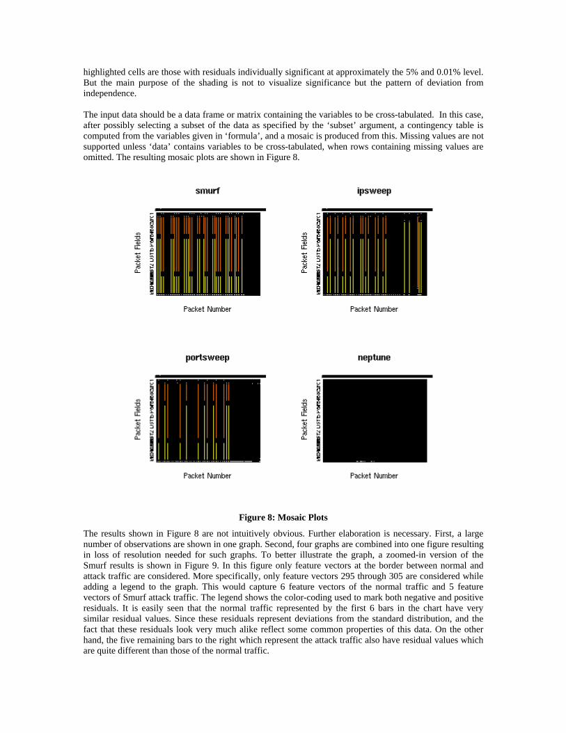
highlighted cells are those with residuals individually significant at approximately the 5% and 0.01% level. But the main purpose of the shading is not to visualize significance but the pattern of deviation from independence. The input data should be a data frame or matrix containing the variables to be cross-tabulated. In this case, after possibly selecting a subset of the data as specified by the ‘subset’ argument, a contingency table is computed from the variables given in ‘formula’, and a mosaic is produced from this. Missing values are not supported unless ‘data’ contains variables to be cross-tabulated, when rows containing missing values are omitted. The resulting mosaic plots are shown in Figure 8.

Figure 8: Mosaic Plots

The results shown in Figure 8 are not intuitively obvious. Further elaboration is necessary. First, a large number of observations are shown in one graph. Second, four graphs are combined into one figure resulting in loss of resolution needed for such graphs. To better illustrate the graph, a zoomed-in version of the Smurf results is shown in Figure 9. In this figure only feature vectors at the border between normal and attack traffic are considered. More specifically, only feature vectors 295 through 305 are considered while adding a legend to the graph. This would capture 6 feature vectors of the normal traffic and 5 feature vectors of Smurf attack traffic. The legend shows the color-coding used to mark both negative and positive residuals. It is easily seen that the normal traffic represented by the first 6 bars in the chart have very similar residual values. Since these residuals represent deviations from the standard distribution, and the fact that these residuals look very much alike reflect some common properties of this data. On the other hand, the five remaining bars to the right which represent the attack traffic also have residual values which are quite different than those of the normal traffic.

In the light of these results, an analogous explanation can be given to the graphs of Figure 8. For the Smurf attack the height and the width of each bar in the graph show the relative frequencies of the variables. The attack packets which are the last 300 feature vectors in the data set had a smaller width of the bars and thus were shown as compacted (black) block at the right side of the graph. So the distinction between normal and attack data is easily visualized. Similar explanations are given for the remaining three graphs.

Figure 9: Mosaic Plot for Feature Vectors 295 Through 305 of the Smurf Attack

7.3. Evaluation of Results

From the results obtained using the different methods as applied to the data sets, it is evident that each method gave an interestingly different view of the nature of the data. To be able to effectively compare the results, several factors should be considered. First, the ability of the each method in distinguishing between normal and attack traffic in the context of explanatory multivariate analysis. It should to emphasized that these methods do not have any apriori knowledge of the data, neither that they are trained to know what the structure of the data is. These methods are comparable to unsupervised learning methods in the field of AI and soft computing. To this end, k-means, hierarchical clustering and SOM provided a clear distinction between normal and attack traffic, while the remaining methods did not provide such a clear view. Second, the method’s effectiveness in its visual presentation, that is, in relaying the underlying structure in the data. Several methods performed really well here, most notably the k-means, the SOM and the Mosaic Plots. One of the compelling features of the graphical output for these methods is that the relationship

between the original data to its final transformation is relatively clear. In the case of k-means there is a direct relationship between the packet number and its cluster assignment. In the case of SOM and Mosaic plots the relationship between the packet number and its final representation is somewhat preserved. On the contrary, using the output from PCA and ICA, it is not clear as to the relationship between the packet numbers and the final transformations. Finally, the time each method takes to execute the algorithm. Table 2 shows the execution time of each algorithm. Three times are shown: User time indicates the time (in seconds) consumed for the user process, system time indicates the time consumed by the operating system and the elapsed time indicates the total time consumed by the overall operation. The difference between user time and system time is that user time is the CPU time used while executing instructions in the user space of the calling process, while system time is the CPU time used by the system on behalf of the calling process. It should be noted that the times given include the time for applying the algorithms for all four data sets, the time to generate the graphics related to the method and finally the time to write this information to the disk. From this perspective, the k-means performed best. FastICA, PCA and SOM were next. Stars plot and hierarchical clustering used relatively high user time. Finally, Mosaic plots performed very poorly in terms of their user time.

Algorithm/Time User (s) System (s) Elapsed (s)

k-means 0.31 0.04 0.42Hierarchical 37.02 0.49 38.76SOM 1.94 0.03 2.2PCA 1.28 0.03 1.59fast ICA 1.07 0.02 1.36Stars 9.56 0.4 12.18Mosaic 224.32 2.73 243.46

Table 2 : Algorithms Execution times

With these results, the best overall performance and visualization is achieved using k-means and SOM. The remaining methods provide interesting insights into the data and may be used to supplement the results obtained through k-means and SOM. However they have several performance and visual limitations making them inappropriate for use as a primary method for analyzing network traffic anomalies.

8. References [1] Herman R., Montroll E. “A Manner of Characterizing the Development of Countries”. National

Academy of Science, U.S.A., No. 10, pp. 3019-3023, October 1972 [2] Han H., Lu X. L., Lu J., Chen B., Yong R. L., “Data Mining Aided Signature Discovery in Network-

Based Intrusion Detection Systems”. ACM SIGOPS Operating System Review. Volume 36, Issue 4, October 2002.

[3] Uppuluri P., Sekar R., “Experiences with Specification-Based Intrusion Detection”. Proceedings of the 4th International Symposium on Recent Advances in Intrusion Detection, 2001, pp. 172 – 189

[4] Denning D.E., “An Intrusion Detection Model”. IEEE Transactions on Software Engineering SE-13: 222-232, 1987.

[5] Warrender C, Forest S., Pearlmutter B. “Detecting Intrusions Using System Calls”, Alternate Data Models, 1999.

[6] Schnell, P. “A method for discovering data-groups”, Biometrica 6, 47-48, 1964. [7] Rojas R. “Neural Network: A Systematic Introduction”. Springer, Berlin, 1996. [8] Portony L., Eskin E., Stolfo J. “Intrusion Detection with Unlabeled Data Using Clustering”,

Proceedings of ACM CSS Workshop on Data Mining Applied to Security (DMSA-2001). Philadelphia, PA: November 5-8, 2001

[9] Knowledge Discovery and Data Mining competition, KDD99 CUP Data Set, 1999. http://kdd.ics.uci.edu

[10] Staniford-Chen S., Heberlein L.T., “Holding Intruders Accountable on the Internet”. Proceedings of the Seventh ACM Conference on Computer and Communications Security.

[11] Shah H., Undercoffer J., Joshi A., “Fuzzy Clustering for Intrusion Detection”. FUZZ-IEEE, 2003 [12] Rhodes B., Mahaffey J., Cannady J., “Multiple Self-Organizing Maps for Intrusion Detection”.

Proceedings of the NISSC 2000 conference, Baltimore M.D. 2000. [13] Girardin L., “An Eye on Network Intruder-Administrator Shootouts”. Proceedings of the Workshop on

Intrusion Detection and Network Monitoring, Santa Clara, CA, USA, April 9-12, 1999. [14] Venables W. N., Ripley B.D., “Modern Applied Statistics with S”. Fourth Edition, Springer-Verlag,

2002 [15] Becker R., Chambers J., and Wilks A., “The New S Language”. Chapman & Hall, London, 1988. [16] http://www.sciviews.org/other/benchmark1.htm [17] http://www.scientificweb.com/ncrunch/ncrunch4.pdf [18] Gordon, A.D., “Classification”, Second Edition, 1999, London: Chapman & Hall [19] S-Plus: Guide to Statistics, Volume 2. Insightful Corporation, 2001 [20] Kaufman, L. and Rousseeuw, P.J., “Finding Groups in Data: An Introduction to Cluster Analysis”

New York: 1990 John Wiley & Sons, Inc. [21] Kohonen T., “Self-Organizing Maps”. NewYork, Springer-Verlag, 1995. [22] Hotelling H., “Analysis of a Complex of Statistical Variables into Principal Components”. Journal of

Educational Psychology, 24:417–441, 1933. [23] Duda R., Hart P., Stork D., Pattern Classification. Second Edition, John Wiley & Sons, Inc., 2001 [24] Haykin S., Neural Networks: A Comprehensive Foundation. Second Edition. Prentice Hall Inc., 1999 [25] Skoudis E., Counter Hack: A Step-by-Step Guide to Computer Attacks and Effective Defenses. Prentice

Hall Inc., 2002 [26] McHugh J., "Testing Intrusion Detection Systems: Critique of the 1998 DARPA Intrusion Detection

System Evaluations as Performed by Lincoln Laboratory." ACM Transactions on Information and System Security, Vol. 3, No. 4, November 2000, Pages 262-294

[27] Schonlau M., “The Clustergram: A Graph for Visualizing Hierarchical and non-Hierarchical Cluster Analyses”. The Stata Journal, 2002, 3, pp 316-327

[28] http://www.cis.hut.fi/aapo [29] Meyer D., Zeileis A., Hornik K., “Visualizing Independence using Extended Association Plots”.

Proceedings of the 3rd International Workshop on Distributed Statistical Computing, Vienna, Austria, 2003.