ANALYSIS OF MATERIAL HANDLING SYSTEMSBASED ON DISCRETE TIME DESIGN MODULES

Furmans, KaiOzden, EdaStoll, JudithEpp, Martin

Karlsruhe Institute of Technology

Schmidt, ThorstenMeinhardt, Ingolf

Schulze, FrankTechnical University of Dresden

Abstract

In this paper, we present a method for the performance evaluation ofmaterial handling systems in an early planning stage. We are mappingtypical material handling elements onto stochastic analytical models.Our intention is to build a toolbox of material handling modules thatallows a fast analysis of typical continuous conveying systems. The toolshould enable the identification of bottlenecks and the computation oflead time distributions for intra-logistic systems.

1 Introduction

During the planning phase of a material handling system it is necessary to assure, thatthe design fulfills the operational requirements. A first check can be done by lookingat the utilization of the individual elements of the design. However, this does onlyguarantee that the required throughput can be achieved over time - and it only worksif the system does not suffer from negative feedback which results for instance fromblocking or too long cycle times of vehicles in a closed system. Therefore, queuingmodels have been used as a method to achieve a fast and more accurate way ofdetermining performance figures during the planning phase.

Since 2004, work has been done in Karlsruhe on queuing models in discrete time,which can be combined using operational data for processing times and the output ofpreceding elements as input for succeeding model elements of the material handlingsystem. Several basic elements have been treated analytically which can now be com-bined (Stochastic Finite Elements, see publications of Schleyer, Ozden, Matzka/Stoll,and Furmans between 2004 and 2011). The advantage of these models lies in the fact,

1

that they allow the computation of not only averages but also the distributions ofe.g. waiting times. This type of models requires good program support for the com-putations and modeling, since the amount of data used and created as well as thecomputation itself cannot be handled manually. Scientists as well as practitionerswill only be able to use these mathematically more advanced methods, if there iscomputer supported modeling and computation available.

At TU Dresden, a research effort has been made during the last years, whichwas also focused on modeling large material handling systems by means of queuingnetworks, with an emphasis on computer modeling. The underlying analytical modelwas based on continuous time models. First experiences with practical applicationshave already been made in Dresden. Now the efforts of both research groups havebeen combined, in order to achieve the following targets:

• A suitable modeling methodology should be defined by mapping typical materialhandling elements onto stochastic analytical models

• By mapping models of large material handling systems onto this modelingmethodology, model elements are identified, where a computation algorithmfor the performance figures is not known yet

• These missing algorithms should be developed

• By comparing the results of the analytical evaluation with simulation resultsof the same model, systematic difference should be identified and correctionfactors should be determined

We want to show and discuss our means of modeling and the capability of theperformance calculation tool as well as its integration within the modeling GUI.This will hopefully lead to a further discussion within the community, how to openthe system for other contributors. For many of the currently as necessary identifiedsingle elements, exact algorithms or good approximations are known through the pastwork. The challenge lies now mostly in modeling control strategies and calculatingthe impact, these control strategies have on throughput and throughput (lead) times.

The paper is organized as follows: First, we will present the modular modelingtechnique in section 1, that is based on single design modules. These single designmodules are based on discrete time calculation methods. We will briefly present theidea of discrete time modeling and its advantages in section 2. Section 3 gives anoverview of the results that can be obtained using the modular modeling techniquethat is implemented in a performance calculation tool with a modeling GUI. In section4, we identify the missing algorithms that should be developed in order to be ableto analyze typical material handling systems. For some of the missing algorithms wealready found a solution. This will be demonstrated by modeling and analyzing a

2

4-way-crossing of roller-conveyors under the time-limited service control strategy (seesection 5).

2 Model design of a modular material flow system

For the methodological support of the early planning phase, the idea of a ”designmodule” arises: in the same way as a material flow system is structured in functionalareas and assemblies, the calculation of overall system behavior is also based on cal-culations of its system components [5]. A material flow system is, therefore, regardedas a node-edge model [8]. The nodes represent the components of the material flowsystem. Typical operations in intra-logistic systems are e.g. checking, packaging ormanual handling processes, but also basic operations on the material flow, such asthe branching and merging of goods, quantity changes by collection and distributionprocesses, as well as sorting and buffering of goods.

As the edges in technical systems (e.g. conveyor belts) transfer streams of goods,they transfer, in the mathematical model, information on the material flow in formof discrete probability distributions to the subsequent nodes. In addition, they canreceive other information on such as transport and waiting time distributions for alater evaluation.

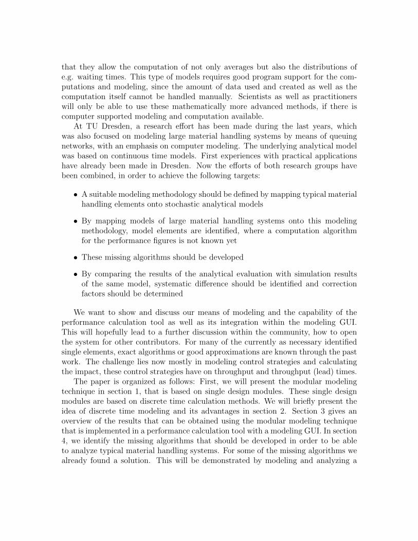
For the modeling process, a multi-level hierarchy is provided, which enables astep-by-step detailing of the required hierarchy level (e.g. storage area, picking areaor similar) down to the individual design module. A design module is a model of aconcrete material flow component (e.g. storage retrieving machine, roller lift table,etc.), which is described based on its functional specification (e.g. steadily / uneven,different service strategies), and with component-specific parameters. In addition,intensity and variability of the incoming transport stream are provided through con-nections from other design modules. Thus, the utilization can be assessed: a highutilization (busy time) of the component can result in queues (and thus waiting time)in front of the module. By means of computational models assigned to the designmodule, the flow behavior after the element is quantified in form of a discrete distri-bution. This distribution is then used as the arrival distribution for the subsequentdesign module (see figure 1).

3 Discrete time methods for the analysis of single designmodules

The analysis tool is based on discrete-time analytical models. Whereas in continuous-time calculation methods (e.g. classical queuing models) characteristic values are cal-culated only on the basis of means and variances, in discrete-time modeling all inputand output variables are described with discrete probability distributions. Thereby

3

Figure 1: Results of modular calculations are mapped to the arriving and departingconveyor lines

the discretization of the time is not a limitation. On the contrary, operational timesin material handling systems exist very often in form of discrete values, such as atransfer carriage, a storage retrieval machine or a turntable.

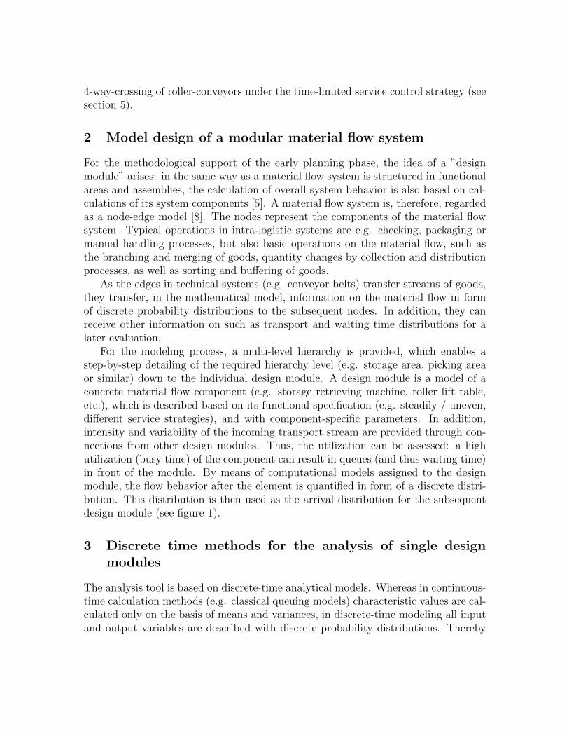
Figure 2 shows this on the example of a carriage with three branch directions andthe associated probability distribution of the service time. In the given example, theconveying time takes only 3 distinct discrete values. The exact, possibly empiricallyobtained values can be used directly as input to the model and do not have to beapproximated by theoretical distributions. Also for the determination of key figures,

Figure 2: Transfer carriage and discrete-time distribution of the direction-dependentcycle times

the discretization is an advantage, because the level of detail is increased essentially.Discrete time modeling enables not only the derivation of mean values but also the

4

quantiles of performance measure, which are often needed for the design of intra-logistic systems. For example, airport baggage handling systems must be designed ina way that arrival baggage is available within a given time on the baggage reclaims.This has to be ensured e.g. with a probability of more than 95%. The same is validfor lead times of picking orders in a distribution center or the required buffer sizein front of a processing station. This is necessary to prevent deadlocks in upstreamareas.

Due to the advantages offered by a discrete time approach, numerous modelsfor the basic elements branching, merging [2], single service station [7], and parallelprocessing stations [4] were developed. In addition, collecting processes and handlingof batches were extensively analyzed ([6], [7]). The past research effort has resultedin a wide range of discrete-time calculation methods.

4 Network analysis based on the modular modeling tech-nique

The analysis of an intra-logistic system begins with the computation of results forthe single components. The analysis tool provides a so-called heat map mode, whichdelivers a quick overview of individual characteristics such as utilization, buffer size,or waiting times. This mode converts the numerical results into a color value whichvisualizes and identifies e.g. the design modules with high utilization or waiting time(Figure 3).

Additional to the probability distributions of the characteristic values for the singledesign modules, discrete distributions of performance measures for a hierarchical level(e.g. in the warehouse: time between triggering the order of stock removal to providein the pre-storage area) or for the complete path through a material flow system canbe obtained easily. For individual transport relations, the distribution of the leadtime can be determined. Moreover, it is also possible to visualize the distributions ofthe pure transport (depending on distance and velocity), service (depending on theprocesses) and waiting times (depending on the workload and working methods) ofthe passed design modules and conveyor lines.

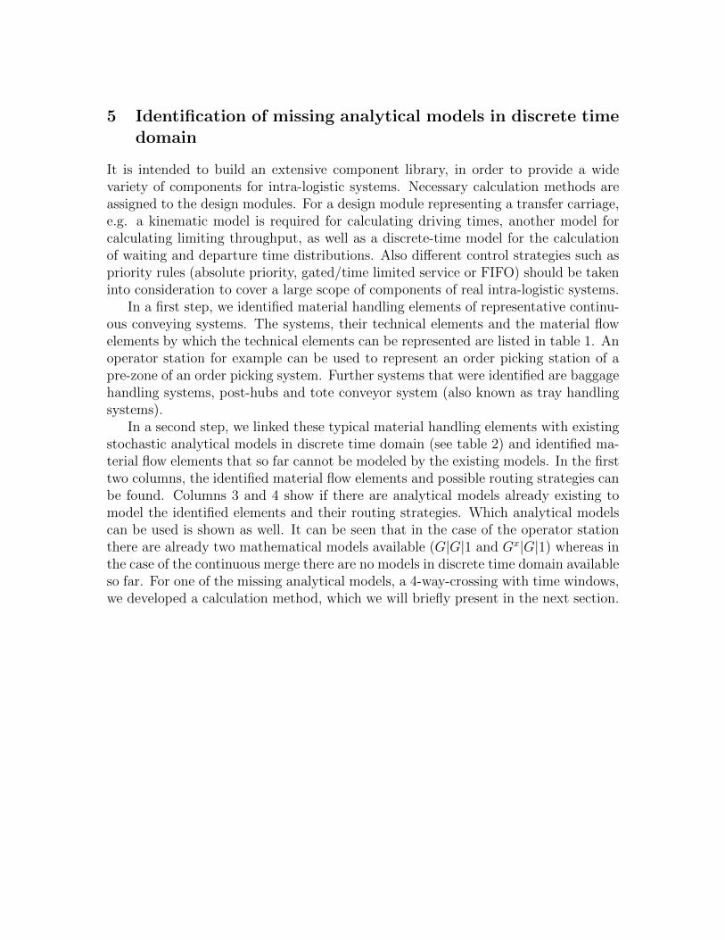
Figure 4 shows the results of an analysis conducted with the analysis tool andvisualizes the mean value and quantiles of the lead time for the investigated system.From the figure, it can be seen that e.g. the 95%-quantile of the lead time has a valueof 399.9 time units. This means that with a 95% probability an order is completedwithin a period of up to 399.9 time units.

5

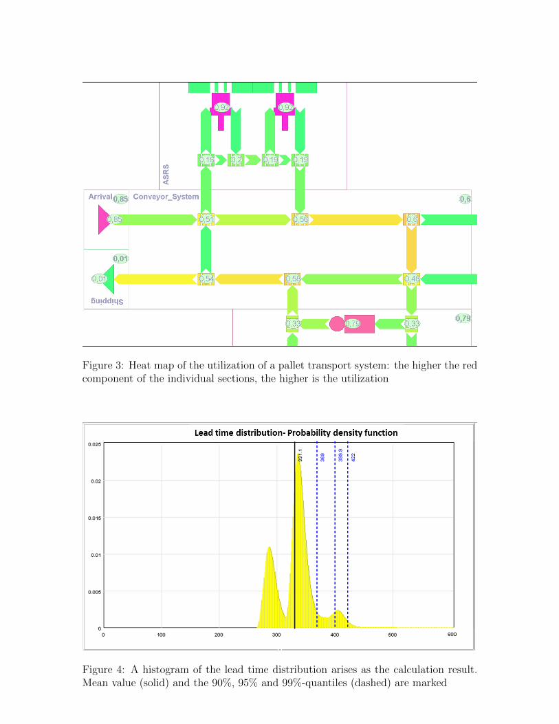
Figure 3: Heat map of the utilization of a pallet transport system: the higher the redcomponent of the individual sections, the higher is the utilization

Figure 4: A histogram of the lead time distribution arises as the calculation result.Mean value (solid) and the 90%, 95% and 99%-quantiles (dashed) are marked

6

5 Identification of missing analytical models in discrete timedomain

It is intended to build an extensive component library, in order to provide a widevariety of components for intra-logistic systems. Necessary calculation methods areassigned to the design modules. For a design module representing a transfer carriage,e.g. a kinematic model is required for calculating driving times, another model forcalculating limiting throughput, as well as a discrete-time model for the calculationof waiting and departure time distributions. Also different control strategies such aspriority rules (absolute priority, gated/time limited service or FIFO) should be takeninto consideration to cover a large scope of components of real intra-logistic systems.

In a first step, we identified material handling elements of representative continu-ous conveying systems. The systems, their technical elements and the material flowelements by which the technical elements can be represented are listed in table 1. Anoperator station for example can be used to represent an order picking station of apre-zone of an order picking system. Further systems that were identified are baggagehandling systems, post-hubs and tote conveyor system (also known as tray handlingsystems).

In a second step, we linked these typical material handling elements with existingstochastic analytical models in discrete time domain (see table 2) and identified ma-terial flow elements that so far cannot be modeled by the existing models. In the firsttwo columns, the identified material flow elements and possible routing strategies canbe found. Columns 3 and 4 show if there are analytical models already existing tomodel the identified elements and their routing strategies. Which analytical modelscan be used is shown as well. It can be seen that in the case of the operator stationthere are already two mathematical models available (G|G|1 and Gx|G|1) whereas inthe case of the continuous merge there are no models in discrete time domain availableso far. For one of the missing analytical models, a 4-way-crossing with time windows,we developed a calculation method, which we will briefly present in the next section.

7

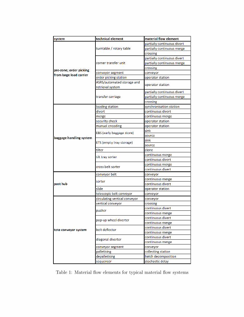
Table 1: Material flow elements for typical material flow systems

8

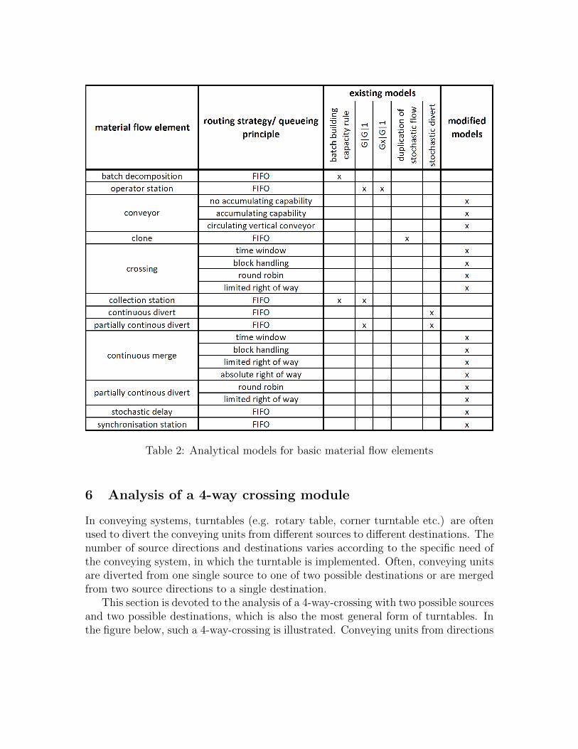
Table 2: Analytical models for basic material flow elements

6 Analysis of a 4-way crossing module

In conveying systems, turntables (e.g. rotary table, corner turntable etc.) are oftenused to divert the conveying units from different sources to different destinations. Thenumber of source directions and destinations varies according to the specific need ofthe conveying system, in which the turntable is implemented. Often, conveying unitsare diverted from one single source to one of two possible destinations or are mergedfrom two source directions to a single destination.

This section is devoted to the analysis of a 4-way-crossing with two possible sourcesand two possible destinations, which is also the most general form of turntables. Inthe figure below, such a 4-way-crossing is illustrated. Conveying units from directions

9

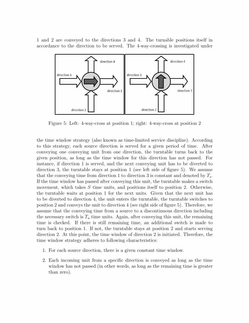
1 and 2 are conveyed to the directions 3 and 4. The turnable positions itself inaccordance to the direction to be served. The 4-way-crossing is investigated under

Figure 5: Left: 4-way-cross at position 1; right: 4-way-cross at position 2

the time window strategy (also known as time-limited service discipline). Accordingto this strategy, each source direction is served for a given period of time. Afterconveying one conveying unit from one direction, the turntable turns back to thegiven position, as long as the time window for this direction has not passed. Forinstance, if direction 1 is served, and the next conveying unit has to be diverted todirection 3, the turntable stays at position 1 (see left side of figure 5). We assumethat the conveying time from direction 1 to direction 3 is constant and denoted by Ts.If the time window has passed after conveying this unit, the turntable makes a switchmovement, which takes S time units, and positions itself to position 2. Otherwise,the turntable waits at position 1 for the next units. Given that the next unit hasto be diverted to direction 4, the unit enters the turntable, the turntable switches toposition 2 and conveys the unit to direction 4 (see right side of figure 5). Therefore, weassume that the conveying time from a source to a discontinuous direction includingthe necessary switch is Tu time units. Again, after conveying this unit, the remainingtime is checked. If there is still remaining time, an additional switch is made toturn back to position 1. If not, the turntable stays at position 2 and starts servingdirection 2. At this point, the time window of direction 2 is initiated. Therefore, thetime window strategy adheres to following characteristics:

1. For each source direction, there is a given constant time window.

2. Each incoming unit from a specific direction is conveyed as long as the timewindow has not passed (in other words, as long as the remaining time is greaterthan zero).

10

3. Conveying of a unit is not interrupted if the time window has elapsed duringits conveying time. The turntable finishes the conveying of this unit and thenpositions itself to the other direction. (As a result, the actual time that theturntable serves a direction can be greater than its time window).

In the next section, the derivation of the queue states is explained.

6.1 Derivation of the queue states

We illustrate here the derivation of the queue state at the beginning of the timewindow of an arbitrary direction. Important variables and parameters used in thisanalysis are listed below:

Ai inter-arrival time at direction iPih transition probability from source direction i to direction hZi time window for direction iCi actual time needed to serve direction iTs conveying time from a source to its continuous direction (e.g. from

direction 1 to direction 3 or from direction 2 to direction 4)Tu conveying time from a source to its discontinuous direction (e.g. from

direction 1 to direction 4 or from direction 2 to direction 3)S switch timeBi service time of a unit from direction iX+i number of conveying units left over at direction i at the end of its time

window.Gi number of conveying units collected at direction i during the time

needed to serve the other directionX i queue state (length), number of conveying units at direction i at the

beginning of its time windowSimilar to the approach presented in [1], we model the turntable as a polling

system, in which one single server serves two queues cyclically, and propose an it-erative algorithm to approximate the queue states. The steps of the algorithm aresummarized as follows.

(1) Initialization: initialize distributions of X+i and Ci and compute the initialX i for i = 1, 2

(2) Recalculate distributions of X+i and Ci based on the computed distributionof X i for i = 1, 2

(3) Recalculate distribution of X i for i = 1, 2

(4) Repeat steps (2)-(3) until a convergence criterion is fulfilled

11

Complying with this algorithm, distributions of queue states are updated in eachiteration step based on their distributions from the previous step. The algorithmterminates when the given convergence criterion is satisfied. A convergence criterioncan be, for instance, the absolute difference between the mean queue state from theactual iteration step and that from the previous iteration step (e.g. we use in ouranalysis | E(X i

n+1)− E(X in) |< 0.0001 as the convergence criterion).

6.2 Initialization

In this step, we compute the service time distributions for both directions. To doso, we introduce the probability P i

s that an arbitrary conveying unit from directioni is conveyed to the continuous direction. Similarly, P i

u is the probability for thediscontinuous direction. They are determined as follows:

P is :=

{P13 if i = 1

P24 if i = 2P iu :=

{P14 if i = 1

P23 if i = 2

Based on the given probabilities, the service time distribution for the conveying unitscan be computed as follows.

P (Bi = Ts) = P is

P (Bi = Tu + S) = P iu

The given service time distribution applies for all conveying units that are handledbefore the last conveying unit in a time window. For such conveying units, theremaining time is always positive. Therefore, the turntable has to position itself to theoriginal position after the unit is conveyed. So, an extra switch time can arise, whichis considered in our analysis as a part of the service time. As a result, the conveyingtime for the continuous direction always equals Ts. In this case, the turntable staysat the original position. For the discontinuous direction, the conveying time is thesum of Tu and switch time S, as the turntable must go back to the original positionafter conveying the unit. However, for the last conveying unit that is handled in atime window, the service time distribution may differ. If the time window has elapsedafter conveying the last unit, the turntable has to position itself to the other source.In this case, a switch has to be made after conveying to the continuous direction,yielding a total service time of (Ts + S) time units, whereas the service time for thediscontinuous direction is Tu.

Subsequently, the distributions of X+i (the number of unit that are left over inthe queue after the time window for the source direction has elapsed) and Ci (totaltime needed to serve the given source direction) are initiated as follows:

P (X+i = 0) = 1 ∀i = 1, 2 (1)

12

P (Ci = Zi) = 1 ∀i = 1, 2 (2)

In order to determine Gi, we firstly introduce an operator, which computes the dis-tribution of the number of arrivals in a given time interval. With this operator, theconditional probability (P (Gi = l | Ci′ = m)), that l arrivals are observed in a timeperiod of m time units, is computed. For different values that the actual time neededto serve the other direction (Ci′ where i′ 6= i), conditional probabilities of Gi arecomputed. With the law of total probability, we attain:

P (Gi = l) =

ci′max∑

m=Zi′

P (Gi = l | Ci′ = m) · P (Ci′ = m) ∀i′ 6= i (3)

where ci′max is the maximum value of Ci′ .

The queue state is the sum of X+i (number of units left over in the queue afterthe time window of the source direction has elapsed) and Gi. Hence, we obtain theinitial queue states (X i) as the convolution of X+i and Gi:

X i = X+i ⊗Gi ∀i = 1, 2 (4)

6.3 Derivation of X+i and Ci

In order to derive the distributions of X+i and Ci, we differentiate between threecases:

Case 1: All units in the queue at the beginning of the time window of a givendirection (X i) are conveyed. Additionally, a part or all of the new arrivalsduring the time window is conveyed.

Case 2: Just a part or all of X i is conveyed during the time window. No newarrival is conveyed either because there was no remaining time left or there wasno new arrival during the time window.

Case 3: There were no units in the queue at the beginning of the time window(X i = 0) and no new arrival occurred during the time window.

For case 1, we introduce the variables arrival time T ij and completion time Ki

j

for each arbitrary j-th arrival within the time window. The arrival time T ij is the

time between the start of a time window and the arrival of the j-th conveying unitfrom the source direction i and Ki

j is the time interval between the start of the timewindow and the completion of service of the j-th unit (see figure 6).

In order to compute the arrival and completion times for new arrivals, we firstlycompute the service completion time for the units already in the queue (X i). For thispurpose, we use the service distribution introduced above, which applies to conveying

13

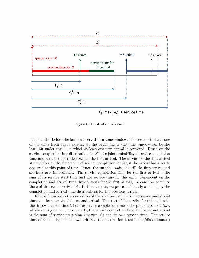
Figure 6: Illustration of case 1

unit handled before the last unit served in a time window. The reason is that noneof the units from queue existing at the beginning of the time window can be thelast unit under case 1, in which at least one new arrival is conveyed. Based on theservice completion time distribution for X i, the joint probability of service completiontime and arrival time is derived for the first arrival. The service of the first arrivalstarts either at the time point of service completion for X i, if the arrival has alreadyoccurred at this point of time. If not, the turnable waits idle till the first arrival andservice starts immediately. The service completion time for the first arrival is thesum of its service start time and the service time for this unit. Dependent on thecompletion and arrival time distributions for the first arrival, we can now computethese of the second arrival. For further arrivals, we proceed similarly and employ thecompletion and arrival time distributions for the previous arrival.

Figure 6 illustrates the derivation of the joint probability of completion and arrivaltimes on the example of the second arrival. The start of the service for this unit is ei-ther its own arrival time (t) or the service completion time of the previous arrival (m),whichever is greater. Consequently, the service completion time for the second arrivalis the sum of service start time (max(m, s)) and its own service time. The servicetime of a unit depends on two criteria: the destination (continuous/discontinuous)

14

of the unit and the remaining time after conveying the unit. We display here thecomputation of the joint probability of completion and arrival time for the j-th unitthat is conveyed to the continuous direction:

P (Kij = (max(m, t) + Ts + x · S) ∧ T i

j = t)

=t−1∑n=1

Zi−1∑m=n+1

P (Kij−1 = m ∧ T i

j−1 = n) · P (Ai = t-n) · P is

where

x =

{1 if (max(m, t) + Ts) ≥ Zi

0 else(5)

In this formula, it is assumed that the previous unit had the arrival time n and thecompletion time m. If the next inter-arrival time has a value (t−n), then the currentunit has the arrival time t and the completion time is the sum of (max(m, t)) and itsservice time. If the unit is conveyed to the continuous direction, its conveying timeis Ts and the probability for this is P i

s . In the formula, we introduced the variable”x”. This variable accounts for the additional switch time needed in the case thatthe time window passed after the unit was conveyed. In this case, the turntable hasto position itself to the reverse source direction after conveying the unit. Therefore,an additional switch time is needed, which is considered in the equation as a part ofthe service time for the conveyed unit. Finally, we consider all the possible values ofm and n. The equation for a unit to be conveyed to the discontinuous direction isderived analogously.

After computing the joint probabilities, we calculate the number of units left overin the queue (X+i) under case 1 by considering two possibilities, in which (X+i > 0).Under the first possibility, an arbitrary j-th arrival happens in t time units andits service is completed in z time units after the start of the time window, wherez ≥ Zi. Consequently, all the new arrivals in time interval (z − t) will be left over.For instance, the third arrival in figure 6 will be left over in the queue. For thispossibility, we compute the number of arrivals within the time interval (z − t).

It is also possible that the service of j-th arrival is completed before the end ofthe time window (z < Zi) and no additional arrival occurs till the end of the timewindow. At the end of the time window, the turntable is still at the original positionand has to switch to the other position, which takes an additional S time units. Ifthere are new arrivals within S time units, these arrivals cannot be conveyed till thenext time window for this direction and have to wait in the queue. Considering thesetwo possibilities, the distribution of X+i is attained.

Thereafter, we compute the actual time needed for direction i (Ci) under the firstcase. We compute the probability that Ci has a value greater than Zi. Ci is greater

15

than Zi if the service completion time of the last unit handled exceeds Zi. Anotherpossibility is that the completion time of the last unit handled was less than Zi and noadditional arrival occurred after this unit. As a result, the turntable positions itself tothe reverse source direction after the time window is over, yielding Ci = Zi+S. Usingjoint probabilities for completion and arrival times, we can compute the distributionof Ci under the first case. Subsequently, X+i and Gi are calculated under cases 2 and3. Afterwards, their distributions can be determined as follows:

for n ≥ 1

P (X+i = n) = P 1(X+i = n) + P 2(X+i = n) + P 3(X+i = n) (6)

where P 1(X+i = n), P 2(X+i = n), and P 3(X+i = n) are the probabilities that X+i

is n units under cases 1, 2, and 3, respectively. Subsequently, it yields:

P (X+i = 0) = 1−∞∑n=1

P (X+i = n) (7)

We proceed similarly for Ci:for p ≥ 1

P (Ci = Zi + p) = P 1(Ci = Zi + p) + P 2(Ci = Zi + p) + P 3(Ci = Zi + p) (8)

P (Ci = Zi) = 1−∞∑p=1

P (Ci = Zi + p) (9)

6.4 Derivation of X i

Eventually, we compute the queue state distribution in the way, as we did in theinitialization. We again compute the distribution of Gi based on the new distributionsof Ci′ (see equation 3) and convolute it with X+i (see equation 4). In this way, weattain the queue state distribution and use it to check the convergence criterion.

6.5 Numerical results

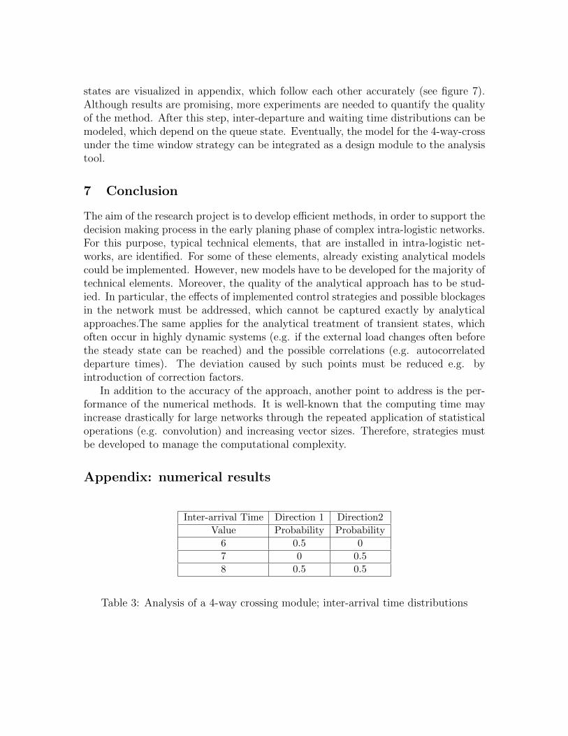
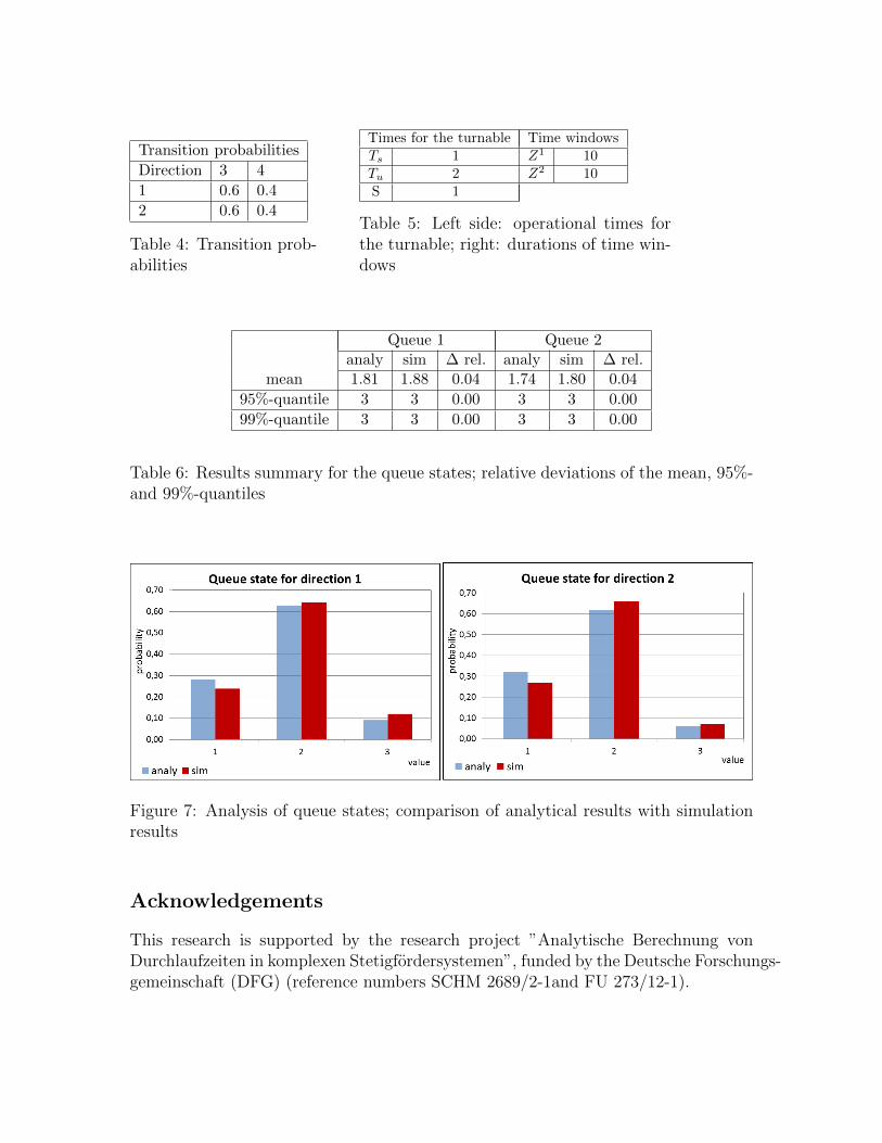
As we have presented an approximate method for the queue states, we discuss herethe quality of the algorithm introduced. For a range of parameters, which are testedup to now, the algorithm yields very accurate results for the higher moments andthe quantiles and generally the computed distributions follow the actual distributionsaccurately. An example is provided in appendix, in which we compare the analyticalresults for queue states with the simulation results (see tables 3 to 5 for inputs).Results for the mean, 95%- and 99%- quantiles as well as relative deviations are dis-played (see table 6). Analytical model delivers the right quantiles. However, the meanvalues show relative deviations of around 4%. Moreover, distributions of the queue

16

states are visualized in appendix, which follow each other accurately (see figure 7).Although results are promising, more experiments are needed to quantify the qualityof the method. After this step, inter-departure and waiting time distributions can bemodeled, which depend on the queue state. Eventually, the model for the 4-way-crossunder the time window strategy can be integrated as a design module to the analysistool.

7 Conclusion

The aim of the research project is to develop efficient methods, in order to support thedecision making process in the early planing phase of complex intra-logistic networks.For this purpose, typical technical elements, that are installed in intra-logistic net-works, are identified. For some of these elements, already existing analytical modelscould be implemented. However, new models have to be developed for the majority oftechnical elements. Moreover, the quality of the analytical approach has to be stud-ied. In particular, the effects of implemented control strategies and possible blockagesin the network must be addressed, which cannot be captured exactly by analyticalapproaches.The same applies for the analytical treatment of transient states, whichoften occur in highly dynamic systems (e.g. if the external load changes often beforethe steady state can be reached) and the possible correlations (e.g. autocorrelateddeparture times). The deviation caused by such points must be reduced e.g. byintroduction of correction factors.

In addition to the accuracy of the approach, another point to address is the per-formance of the numerical methods. It is well-known that the computing time mayincrease drastically for large networks through the repeated application of statisticaloperations (e.g. convolution) and increasing vector sizes. Therefore, strategies mustbe developed to manage the computational complexity.

Appendix: numerical results

Inter-arrival Time Direction 1 Direction2

Value Probability Probability

6 0.5 0

7 0 0.5

8 0.5 0.5

Table 3: Analysis of a 4-way crossing module; inter-arrival time distributions

17

Transition probabilities

Direction 3 4

1 0.6 0.4

2 0.6 0.4

Table 4: Transition prob-abilities

Times for the turnable Time windowsTs 1 Z1 10Tu 2 Z2 10S 1

Table 5: Left side: operational times forthe turnable; right: durations of time win-dows

Queue 1 Queue 2analy sim ∆ rel. analy sim ∆ rel.

mean 1.81 1.88 0.04 1.74 1.80 0.04

95%-quantile 3 3 0.00 3 3 0.00

99%-quantile 3 3 0.00 3 3 0.00

Table 6: Results summary for the queue states; relative deviations of the mean, 95%-and 99%-quantiles

Figure 7: Analysis of queue states; comparison of analytical results with simulationresults

Acknowledgements

This research is supported by the research project ”Analytische Berechnung vonDurchlaufzeiten in komplexen Stetigfordersystemen”, funded by the Deutsche Forschungs-gemeinschaft (DFG) (reference numbers SCHM 2689/2-1and FU 273/12-1).

18

8 References

[1] Dittmann, R. and Hubner, F. ”Discrete-Time Analysis of a Cyclic Service Systemwith Gated Limited Service”. Technical report, Lehrstuhl fur Informatik, UniversitatWurzburg (1993)

[2] Furmans, K. ”A framework of stochastic finite elements for models of mate-rial handling systems”. Progress in Material Handling Research. 8th InternationalMaterial Handling Research Colloquium, Graz (2004)

[3] Grassmann, W. K.; Jain, J. L. ”Numerical solutions of the waiting time dis-tribution and idle time distribution of the arithmetic GI/G/1 queue”. OperationsResearch 37 (1), 141-150 (1989)

[4] Matzka, J. ”Discrete Time Analysis of Multi-Server Queueing Systems in Ma-terial Handling and Service”. PhD Thesis. Karlsruhe Institute of Technology (2011)

[5] Meinhardt, I. and Marquardt, H.-G. ”Offenes Baukastensystem zur effizien-ten Dimensionierung von Materialflusssystemen”. Final report of research project.Technical University Dresden (2006)

[6] Ozden, E. ”Discrete time Analysis of Consolidated Transport Processes”. PhDThesis. Karlsruhe Institute of Technology (2011)

[7] Schleyer, M. ”Discrete Time Analysis of Batch Processes in Material FlowSystems”. PhD Thesis. Karlsruhe University (2007)

[8] Schmidt, T. ”Schnelle Materialfluss-Planung bei veranderlichen Parametern.”Strukturwandel in der Logistik : Wissenschaft und Praxis im Dialog : 5. BVLWissenschaftssymposium Logistik, S. 32-46 (2010)

[9] Tran-Gia, P. ”Analytische Leistungsbewertung verteilter Systeme”. Springer(1996)

19