Analysis of localized solutions in coupled Gross-Pitaevskii...
193
Analysis of localized solutions in coupled Gross-Pitaevskii equations Muhammad Irfan Qadir Thesis submitted to The University of Nottingham for the degree of Doctor of Philosophy October 2013
Transcript of Analysis of localized solutions in coupled Gross-Pitaevskii...

Analysis of localized solutions in
coupled Gross-Pitaevskii equations
Muhammad Irfan Qadir
Thesis submitted to The University of Nottingham
for the degree of Doctor of Philosophy
October 2013

Dedicated to my beloved parents
who did many dua’s for me!
i

Abstract
Bose-Einstein condensates (BECs) have been one of the most active areas of research
since their experimental birth in 1995. The complicated nature of the experiments on
BECs suggests to observe them in reduced dimensions. The dependence of the collec-
tive excitations of the systems on the spatial degrees of freedom allows the study in
lower dimensions. In this thesis, we first study two effectively one-dimensional par-
allel linearly coupled BECs in the presence of external potentials. The system is mod-
elled by linearly coupled Gross-Pitaevskii (GP) equations. In particular, we discuss
the dark solitary waves and the grey-soliton-like solutions representing analogues of
superconducting Josephson fluxons which we refer to as the fluxon analogue (FA) so-
lutions. We analyze the existence, stability and time dynamics of FA solutions and
coupled dark solitons in the presence of a harmonic trap. We observe that the presence
of the harmonic trap destabilizes the FA solutions. However, stabilization is possible
by controlling the effective linear coupling between the condensates. We also derive
theoretical approximations based on variational formulations to study the dynamics of
the solutions semi-analytically.
We then study multiple FA solutions and coupled dark solitons in the same settings. We
examine the effects of trapping strength on the existence and stability of the localized
solutions. We also consider the interactions of multiple FA solutions as well as coupled
dark solitons. In addition, we determine the oscillation frequencies of the prototypical
structures of two and three FA solutions using a variational approach.
Finally, we consider two effectively two-dimensional parallel coupled BECs enclosed
in a double well potential. The system is modelled by two GP equations coupled by
linear and nonlinear cross-phase-modulations. We study a large set of radially sym-
metric nonlinear solutions of the system in the focusing and defocusing cases. The
relevant three principal branches, i.e. the ground state and the first two excited states,
are continued as a function of either linear or nonlinear couplings. We investigate the
linear stability and time evolution of these solutions in the absence and presence of a
topological charge. We notice that only the chargeless or charged ground states can be
ii

stabilized by adjusting the linear or nonlinear coupling between the condensates.
iii
Publications
Most of the work of this thesis has been published or going to appear for publication.
1. Parts of Chapter 3 in this thesis have been published in:
M. I. Qadir, H. Susanto and P. C. Matthews, Fluxon analogues and dark solitons
in linearly coupled Bose-Einstein condensates, J. Phys. B: At. Mol. Opt. Phys. 45,
035004 (2012).
2. Parts of Chapter 4 in this thesis have appeared as a chapter in:
M. I. Qadir, H. Susanto and P. C. Matthews, Multiple fluxon analogues and dark
solitons in linearly coupled Bose-Einstein condensates. In B. A. Malomed (Ed),
Spontaneous Symmetry Breaking, Self-Trapping, and Josephson Oscillations in
Nonlinear Systems (Springer, Berlin, 2013), 485 − 508.
iv

Acknowledgements
First of all, I praise and say bundle of thanks to Almighty Allah, the Most Gracious and
the Most Merciful. Certainly, it is just due to His mercy, favours and bounties that I
have completed this thesis.
I was fortunate to have Dr. Hadi Susanto and Dr. Paul Matthews as my supervisors
who provided me invaluable guidance throughout my PhD studies. Their knowledge
and way of thinking and doing work always inspired me. I feel honoured while getting
benefits from their knowledge and mathematical experience. So, I would like to offer
my sincerest gratitude and thanks to both of them who have supported me throughout
my PhD studies with their patience and knowledge. I am grateful for their suggestions
during my studies, including their comments and corrections on the manuscripts of
the thesis.
Next, I would like to express my heartiest gratitude to my father Ghulam Qadir and
my mother Bushra Bibi for their moral support and encouragement during my studies.
Their continuous prayers brought me to this stage. My sincere thanks go to my brothers
Muhammad Imran Qadir, Rizwan Qadir, Adnan Qadir, my sisters-in-law, my nephew
Hamza Imran and my nieces for their encouragement and prayers.
Special thanks goes to Dr. Muhammad Ozair Ahmad Chairman of the Department of
Mathematics, University of Engineering and Technology, Lahore, who helped me a lot
in getting funded every year during my stay in England.
It is a pleasure to single out Dr. Mahdhivan Syafwan, Dr. Mainul Haq and Dr. Hafiz
Saeed Ahmad for their support, help and warm brotherhood. There are many other
people who supported and encouraged me during my PhD studies. To list all of them
is, of course, not possible here but I acknowledge all of them. Finally, I am thankful
to the University of Engineering and Technology, Lahore, Pakistan for providing me
financial support.
v

List of Abbreviations
KdV Korteweg-de Vries (Equation)
IST Inverse Scattering Transform
NLS Nonlinear Schrödinger (Equation)
GL Ginzburg-Landau (Equation)
BEC Bose-Einstein Condensate
JILA Joint Institute for Laboratory Astrophysics
MIT Massachusetts Institute of Technology
GP Gross-Pitaevskii (Equation)
BJJ Bose-Josephson Junction
FA Fluxon Analogues
JV Josephson Vortices
vi

Contents
1 Introduction 1
1.1 Bose-Einstein condensate (BEC) and subatomic particles . . . . . . . . . 4
1.2 Bose-Einstein condensation . . . . . . . . . . . . . . . . . . . . . . . . . . 5
1.3 Phases of matter . . . . . . . . . . . . . . . . . . . . . . . . . . . . . . . . . 6
1.4 Formation of BEC by Laser cooling technique . . . . . . . . . . . . . . . . 6
1.5 Characteristics and future applications of BECs . . . . . . . . . . . . . . . 7
1.6 The external potential . . . . . . . . . . . . . . . . . . . . . . . . . . . . . . 8
2 Mathematical Background 10
2.1 The variational approximations . . . . . . . . . . . . . . . . . . . . . . . . 10
2.2 The Gross-Pitaevskii equation . . . . . . . . . . . . . . . . . . . . . . . . . 11
2.3 Ground state and Thomas-Fermi approximation . . . . . . . . . . . . . . 15
2.4 Dimensionality reduction in GP models . . . . . . . . . . . . . . . . . . . 16
2.5 Dimensionless form of GP equation . . . . . . . . . . . . . . . . . . . . . 18
2.6 Solutions of one-dimensional GP equations and their stability . . . . . . 19
2.6.1 The plane-wave solution . . . . . . . . . . . . . . . . . . . . . . . . 19
2.6.2 Matter wave dark solitons . . . . . . . . . . . . . . . . . . . . . . . 22
2.6.2.1 The stability of dark solitons . . . . . . . . . . . . . . . . 25
2.6.2.2 The stability of dark solitons in the inhomogeneous case 29
2.6.2.3 Travelling dark solitons . . . . . . . . . . . . . . . . . . . 30
2.6.2.4 The stability of travelling dark soliton solution . . . . . 31
2.6.3 Matter wave bright solitons and their stability . . . . . . . . . . . 32
2.7 Multi-component BECs and coupled system of Gross-Pitaevskii equations 33
vii

CONTENTS
2.7.1 Two-mode representations of the GP equation . . . . . . . . . . . 34
2.8 Vortices in optics and BECs . . . . . . . . . . . . . . . . . . . . . . . . . . 36
2.9 Overview of the thesis . . . . . . . . . . . . . . . . . . . . . . . . . . . . . 37
3 Fluxon analogues and dark solitons in linearly coupled Bose-Einstein con-
densates 40
3.1 Introduction . . . . . . . . . . . . . . . . . . . . . . . . . . . . . . . . . . . 40
3.2 Overview of the chapter . . . . . . . . . . . . . . . . . . . . . . . . . . . . 42
3.3 Fluxon analogues solution . . . . . . . . . . . . . . . . . . . . . . . . . . . 43
3.4 Numerical computations . . . . . . . . . . . . . . . . . . . . . . . . . . . . 43
3.4.1 Coupled one-dimensional GP equations with k > 0 and V = 0 . . 43
3.4.2 Stability of dark soliton in coupled one-dimensional GP equations 44
3.4.3 Existence of fluxon analogues solution . . . . . . . . . . . . . . . . 48
3.4.4 Stability of fluxon analogues solution . . . . . . . . . . . . . . . . 48
3.4.5 Coupled BECs with a trap: V = 0 . . . . . . . . . . . . . . . . . . 49
3.5 Travelling FA solutions and the velocity dependence of the critical cou-
pling kce . . . . . . . . . . . . . . . . . . . . . . . . . . . . . . . . . . . . . 55
3.6 Variational formulations of the FA solutions . . . . . . . . . . . . . . . . . 60
3.6.1 The case k ∼ kce and V = 0 . . . . . . . . . . . . . . . . . . . . . . 60
3.6.2 The case k ∼ 0 and V = 0 . . . . . . . . . . . . . . . . . . . . . . . 65
3.7 Conclusion . . . . . . . . . . . . . . . . . . . . . . . . . . . . . . . . . . . . 66
4 Multiple fluxon analogues and dark solitons in linearly coupled Bose-Einstein
condensates 68
4.1 Introduction . . . . . . . . . . . . . . . . . . . . . . . . . . . . . . . . . . . 68
4.2 Overview of the chapter . . . . . . . . . . . . . . . . . . . . . . . . . . . . 69
4.3 Variational approximations . . . . . . . . . . . . . . . . . . . . . . . . . . 70
4.3.1 Determining the interaction potential . . . . . . . . . . . . . . . . 70
4.3.2 Variational approximation for multiple FA solutions . . . . . . . . 72
4.3.2.1 Lagrangian approach for finding the oscillation frequency
of two FA solutions . . . . . . . . . . . . . . . . . . . . . 72
viii

CONTENTS
4.3.2.2 Lagrangian approach for finding the oscillation frequency
of three FA solutions . . . . . . . . . . . . . . . . . . . . 74
4.4 Numerical simulations and computations . . . . . . . . . . . . . . . . . . 76
4.4.1 Interactions of uncoupled dark solitons without trap . . . . . . . 76
4.4.2 Interaction of dark solitons in coupled NLS equations without trap 77
4.4.3 Interaction of FA solutions in the absence of a magnetic trap . . . 79
4.4.4 Stationary multiple FA solutions and dark solitons in the pres-
ence of magnetic trap . . . . . . . . . . . . . . . . . . . . . . . . . . 83
4.4.4.1 (+−)-configuration of FA . . . . . . . . . . . . . . . . . . 90
4.4.4.2 (++)-configuration of FA . . . . . . . . . . . . . . . . . . 95
4.4.4.3 (+−+)-configuration of FA . . . . . . . . . . . . . . . . 96
4.4.4.4 (+++)-configuration of FA . . . . . . . . . . . . . . . . 97
4.5 Conclusion . . . . . . . . . . . . . . . . . . . . . . . . . . . . . . . . . . . . 104
5 Radially symmetric nonlinear states of coupled harmonically trapped Bose-
Einstein condensates 105
5.1 Introduction . . . . . . . . . . . . . . . . . . . . . . . . . . . . . . . . . . . 105
5.2 Overview of the chapter . . . . . . . . . . . . . . . . . . . . . . . . . . . . 106
5.3 Theoretical setup and numerical methods . . . . . . . . . . . . . . . . . . 107
5.4 Numerical results . . . . . . . . . . . . . . . . . . . . . . . . . . . . . . . . 109
5.4.1 Stability analysis of the nonlinearly coupled system . . . . . . . . 110
5.4.2 Stability analysis of the linearly coupled system . . . . . . . . . . 143
5.4.3 Stability analysis in the presence of linear and nonlinear coupling 143
5.4.4 Stability analysis in case of unequal vorticity in the two compo-
nents of BECs . . . . . . . . . . . . . . . . . . . . . . . . . . . . . . 144
5.5 Conclusion . . . . . . . . . . . . . . . . . . . . . . . . . . . . . . . . . . . . 144
6 Conclusion and Future Work 155
6.1 Summary . . . . . . . . . . . . . . . . . . . . . . . . . . . . . . . . . . . . . 155
6.2 Future work . . . . . . . . . . . . . . . . . . . . . . . . . . . . . . . . . . . 159
References 161
ix

List of Figures
2.1 Numerically obtained solutions (solid) of the stationary GP Eq. (2.3.1) in
a spherical trap with repulsive interatomic interaction corresponding toNaaho
= 1, 10, 100. The dashed curve represents the prediction for the ideal
gas. Figure has taken from [69]. . . . . . . . . . . . . . . . . . . . . . . . . 16
2.2 The plot of the Thomas-Fermi approximation (2.3.3) with the harmonic
potential V = 12 Ω2x2. Here, Ω = 0.1, ρ0 = 1 and g = 1. . . . . . . . . . . 17
2.3 Plot of a black soliton (black) with parameter values A = 1, B = v = 0
and a grey soliton (blue) with A =√
32 , B = v = 0.5. . . . . . . . . . . . . 23
2.4 A numerically obtained dark soliton solution. The blue curve represents
the real part while the black horizontal line represents the imaginary part
of the solution. . . . . . . . . . . . . . . . . . . . . . . . . . . . . . . . . . . 26
2.5 The structure of the eigenvalues in the complex plane for the solution
shown in Fig. 2.4. . . . . . . . . . . . . . . . . . . . . . . . . . . . . . . . . 28
2.6 Contour plot obtained through the direct numerical integration of Eq.
(2.6.26) depicting the time evolution of the dark soliton solution shown
in Fig. 2.4. . . . . . . . . . . . . . . . . . . . . . . . . . . . . . . . . . . . . 28
2.7 The profiles of a dark soliton in the presence of the magnetic trap with
trapping strength Ω = 0.05, 0.1, 0.15, 0.2 respectively. In each figure the
blue curve represents the real part while the black horizontal line repre-
sents the imaginary part of the solution. The higher the value of Ω, the
smaller the width of the dark soliton. . . . . . . . . . . . . . . . . . . . . . 29
2.8 The structure of the eigenvalues in the complex plane for the dark soliton
in the presence of the magnetic trap with Ω = 0.1. . . . . . . . . . . . . . 30
2.9 Contour plot obtained through the direct numerical integration of Eq.
(2.6.25) depicting the time evolution of the dark soliton solution shown
in Fig. 2.7. . . . . . . . . . . . . . . . . . . . . . . . . . . . . . . . . . . . . 31
x

LIST OF FIGURES
2.10 Contour plot obtained through the direct numerical integration of Eq.
(2.6.11) depicting the time evolution of the bright soliton solution shown
in Fig. 2.11. . . . . . . . . . . . . . . . . . . . . . . . . . . . . . . . . . . . . 33
2.11 Comparison between the untrapped (blue) and the trapped (black dashed)
bright solitons. For the trapped bright soliton, Ω = 0.2. Both graphs are
almost same showing that the magnetic trap does not affect the stability
of the solution. . . . . . . . . . . . . . . . . . . . . . . . . . . . . . . . . . . 34
3.1 A sketch of the problem in the context of Bose-Einstein condensates,
which are strongly confined in the y− and z−direction and elongated
along the x−direction. . . . . . . . . . . . . . . . . . . . . . . . . . . . . . 41
3.2 Spatial profile of the phase difference between Ψ1 and Ψ2 of FA solution
for k = 0.1 forming a 2π-kink shape. . . . . . . . . . . . . . . . . . . . . . 44
3.3 Numerical solution of two coupled one-dimensional GP equations for
µ = 1, ρ0 = 1, k = 0.3, ∆x = 0.2. The blue curves represent the real
parts and the black horizontal lines represent the imaginary parts of the
solution. . . . . . . . . . . . . . . . . . . . . . . . . . . . . . . . . . . . . . 45
3.4 The eigenvalues λ of the solution in Fig. 3.3 in the complex plane show-
ing the instability of the solution. . . . . . . . . . . . . . . . . . . . . . . . 46
3.5 The critical eigenvalue of coupled dark solitons shown in Fig. 3.3 as a
function of k. . . . . . . . . . . . . . . . . . . . . . . . . . . . . . . . . . . . 46
3.6 An evolution of the unstable coupled dark solitons shown in Fig. 3.3.
The left panel corresponds to |Ψ1| and right panel to |Ψ2|. . . . . . . . . . 47
3.7 Time evolution of the unstable coupled dark solitons shown in Fig. 3.3
for few particular values of time. . . . . . . . . . . . . . . . . . . . . . . . 47
3.8 A numerically obtained FA for ρ0 = 1, µ = 1, and k = 0.1. The blue
curves represent the real parts while the black curves are the imaginary
parts of Ψ1 and Ψ2, respectively. . . . . . . . . . . . . . . . . . . . . . . . 48
3.9 The hump amplitude of the imaginary parts of FA solution shown in Fig.
3.8 against k. The graph depicts the region of existence of FA solution.
The blue and black curves correspond to the imaginary parts of Ψ1 and
Ψ2 while the red line in the middle is for the coupled dark solitons. . . . 49
3.10 The eigenvalues distribution of the FA for k = 0.1 in the complex plane
showing the stability of the solution. . . . . . . . . . . . . . . . . . . . . . 50
xi

LIST OF FIGURES
3.11 Time dynamics of the coupled dark solitons when the coupling between
them is very small and the two coupled dark solitons repel each other.
The left panel corresponds to |Ψ1| and right panel to |Ψ2|. Here, k =
0.001. . . . . . . . . . . . . . . . . . . . . . . . . . . . . . . . . . . . . . . . 50
3.12 A numerically obtained FA solution for Ω = 0.1, ρ0 = 1, µ = 1 and
k = 0.1. The blue solid curves represent the real parts and the black
solid curves are the imaginary parts of the FA solution. The dash-dotted
curves are approximations (see Section 3.6, Eq. (3.6.1)). . . . . . . . . . . 51
3.13 A numerically obtained FA solution for the same parameter values as in
Fig. 3.12 but k = 0.008. The blue solid curves represent the real parts
and the black solid curves are the imaginary parts of the FA solution.
The dash-dotted curves and the dashed curves are two approximations
obtained through different approaches (see Section 3.6, Eqs. (3.6.1) and
(3.6.19) respectively). . . . . . . . . . . . . . . . . . . . . . . . . . . . . . . 51
3.14 A numerically obtained coupled dark soliton for Ω = 0.1, ρ0 = 1, µ = 1
and k = 0.4. The blue curves represent the real parts and the black
horizontal lines are the imaginary parts of the solitons. . . . . . . . . . . 52
3.15 Eigenvalues structures for the FA solutions shown in Fig. 3.12 and Fig.
3.13 respectively. A pair of eigenvalues in both panels is lying on the
vertical axis showing the instability of the solutions. . . . . . . . . . . . . 53
3.16 The first few lowest squared eigenvalues of FA (solid) and dark solitons
(dashed) as a function of k for Ω = 0.1. The dash-dotted curve represents
the approximation (3.6.17). . . . . . . . . . . . . . . . . . . . . . . . . . . 54
3.17 Eigenvalues structure showing the stability of the FA solution for Ω =
0.1 and k = 0.2. . . . . . . . . . . . . . . . . . . . . . . . . . . . . . . . . . 54
3.18 Stability curves for FA solutions corresponding to Ω = 0.05, 0.1, 0.15, 0.2.
For each value of Ω, there is a little change in the value of kcs. . . . . . . 55
3.19 The upper panel shows a numerical evolution of the FA in Fig. 3.12 for
Ω = 0.1 and k = 0.1. The lower panel shows a numerical evolution of
the phase difference for the same parameter values above. The phase
changes from −2π to 0 and shows the presence of FA solution. . . . . . . 56
3.20 A numerical evolution of coupled dark solitons for Ω = 0.1 and k = 0.1. 57
3.21 A numerically obtained FA for v = 0.2 and k = 0.1. . . . . . . . . . . . . 59
xii

LIST OF FIGURES
3.22 The critical coupling constant kce as a function of the velocity v for the
existence of travelling FA. Filled circles are numerical data and the solid
line is the function in Eq. (3.5.10). FA only exists on the left of the solid
curve. . . . . . . . . . . . . . . . . . . . . . . . . . . . . . . . . . . . . . . 59
3.23 Time dynamics of the travelling coupled dark solitons and the travelling
FA for the parameter values k = 0.1 and v = 0.2. The upper panel shows
the instability of the coupled dark solitons and the lower panel depicts
the stability of travelling FA solution. . . . . . . . . . . . . . . . . . . . . 61
4.1 Numerical evolutions of interaction of two dark solitons. The solitons
are moving with velocities v1 = −v2 = 0.1. The interparticle repulsion
is dominant over the kinetic energies of solitons and solitons are going
away from each other after interaction. The white solid curves are simu-
lations of trajectories of solutions obtained through Eq. (4.3.9). Note that
an exact analytic solution is given by (4.1.2). . . . . . . . . . . . . . . . . 77
4.2 Numerical evolutions of interaction of two dark solitons. The solitons
are moving with velocities v1 = −v2 = 0.6. The interparticle repulsion
is suppressed by the kinetic energies of the solitons and they transmit
through each other at the interacting point. The white solid curves are
simulations of trajectories of solutions obtained through Eq. (4.3.9). The
exact analytic solution is given by (4.1.2). . . . . . . . . . . . . . . . . . . 78
4.3 Numerical evolutions of interaction of two dark solitons. One of the
solitons is static and the other is moving with velocity v = 0.5. After
interaction, the travelling soliton becomes stationary and the static soli-
ton starts moving with the velocity of the other soliton. The white solid
curves are simulations of trajectories of solutions obtained through Eq.
(4.3.9). . . . . . . . . . . . . . . . . . . . . . . . . . . . . . . . . . . . . . . 78
4.4 Numerical evolutions of interaction of two coupled dark solitons for
k = 0.1. The solitons are moving with velocities v1 = −v2 = 0.2. The
interparticle repulsion is dominant over the kinetic energies and the soli-
tons are going away from each other after interaction. Due to an insta-
bility, they break down at approximately t = 120. The white solid curves
are simulations of trajectories of solutions obtained through Eq. (4.3.9). 80
xiii

LIST OF FIGURES
4.5 Numerical evolutions of interaction of two coupled dark solitons for
k = 0.1. The solitons are moving with velocities v1 = −v2 = 0.6. The in-
terparticle repulsion is suppressed by the kinetic energies of the solitons
and they transmit through each other at the interacting point. The white
solid curves are simulations of trajectories of solutions obtained through
Eq. (4.3.9). . . . . . . . . . . . . . . . . . . . . . . . . . . . . . . . . . . . . 80
4.6 Numerical evolutions of interaction of two coupled dark solitons for k =
0.1. One of the coupled solitons is static and the other is moving with
velocity v = 0.5. The white solid curves are simulations of trajectories of
solutions obtained through Eq. (4.3.9). . . . . . . . . . . . . . . . . . . . . 81
4.7 Numerical evolutions of collision of three coupled dark solitons for k =
0.1. Two solitons are moving with velocities v1 = −v3 = 0.2 and the
soliton between these moving solitons is at rest, i.e. v2 = 0. The inter-
particle repulsion is dominant over the kinetic energies and the solitons
are going away from each other after interaction. The break up is due to
the instability of the travelling dark solitons. . . . . . . . . . . . . . . . . 81
4.8 Numerical evolutions of collision of three coupled dark solitons for k =
0.1. The solitons are moving with velocities v1 = −v2 = 0.6 and v2 =
0. The interparticle repulsion is suppressed by the kinetic energies of
the solitons and the moving solitons transmit through each other at the
interacting point leaving the static soliton undisturbed. . . . . . . . . . . 82
4.9 Profiles of an initial condition representing two coupled FA solutions
travelling with velocities v1 = −v2 = 0.2 corresponding to k = 0.1. The
figure in the upper panel represents the odd interaction referred to as
(+−)-configuration, while figure in the lower panel is the even interac-
tion and referred to as (++)-configuration of FA solution. . . . . . . . . 84
4.10 As Fig. 4.1, but for the odd symmetric collision of FA solutions for v =
0.2 and k = 0.1. . . . . . . . . . . . . . . . . . . . . . . . . . . . . . . . . . 85
4.11 As Fig. 4.1, but for the odd symmetric collision of FA solutions for v =
0.6 and k = 0.1. . . . . . . . . . . . . . . . . . . . . . . . . . . . . . . . . . 85
4.12 As Fig. 4.1, but the even symmetric collision of FA solutions for v = 0.1
and k = 0.1. . . . . . . . . . . . . . . . . . . . . . . . . . . . . . . . . . . . 86
4.13 As Fig. 4.1, but the even symmetric collision of FA solutions for v = 0.2
and k = 0.1. . . . . . . . . . . . . . . . . . . . . . . . . . . . . . . . . . . . 86
xiv
LIST OF FIGURES
4.14 As Fig. 4.1, but the even symmetric collision of FA solutions for v = 0.6
and k = 0.1. . . . . . . . . . . . . . . . . . . . . . . . . . . . . . . . . . . . 87
4.15 Numerical evolutions of the odd symmetric collisions of two FA solu-
tions when one of them is static while the other is moving with velocity
v = 0.2 and k = 0.1. . . . . . . . . . . . . . . . . . . . . . . . . . . . . . . 87
4.16 Numerical evolutions of the odd symmetric collisions of two FA solu-
tions when one of them is static while the other is moving with velocity
v = 0.6 and k = 0.1. . . . . . . . . . . . . . . . . . . . . . . . . . . . . . . 88
4.17 As Fig. 4.15, but the even symmetric collision of FA solutions for v = 0.2
and k = 0.1. . . . . . . . . . . . . . . . . . . . . . . . . . . . . . . . . . . . 88
4.18 As Fig. 4.15, but the even symmetric collision of FA solutions for v = 0.6
and k = 0.1. . . . . . . . . . . . . . . . . . . . . . . . . . . . . . . . . . . . 89
4.19 Numerical evolutions of collision of three FA solutions for k = 0.1. Two
FA solutions are moving with velocities v1 = −v3 = 0.2 and the FA
solution in the middle is at rest. . . . . . . . . . . . . . . . . . . . . . . . 89
4.20 Numerical evolutions of collision of three FA solutions for k = 0.1. Two
FA solutions are moving with velocities v1 = −v3 = 0.6 and the other
one is at rest. The FA solutions are indistinguishable after the interaction. 90
4.21 Numerically obtained multiple FA with a (+−)-configuration for Ω =
0.1, ρ0 = 1, k = 0.2. . . . . . . . . . . . . . . . . . . . . . . . . . . . . . . . 91
4.22 Graph of Ω and kce for the (+−)-configuration of FA solution. The curve
shows the dependence of kce on the trapping strength Ω. . . . . . . . . . 92
4.23 Coupled dark soliton solutions for Ω = 0.1, ρ0 = 1, k = 0.5. . . . . . . . . 92
4.24 Graph of Ω and kcs for the (+−)-configuration of FA solution. The curve
shows the dependence of kcs on the trapping strength Ω. . . . . . . . . . 93
4.25 The eigenvalue structure of the soliton in Fig. 4.21 in the complex plane. 93
4.26 The spectrum of eigenvalues in the middle for Ω = 0.1 and k = 0.5
showing the stability of the solution shown in Fig. 4.23. . . . . . . . . . . 94
4.27 The graph of k and the maximum imaginary parts of eigenvalues for
Ω = 0.1. The solid and dashed curves represent the trajectories of the
most unstable eigenvalue for FA and dark soliton as a function of k re-
spectively. The dash-dotted curve represents the approximation (4.3.19)
for the oscillation frequency of the (+−)-configuration of FA. . . . . . . . 94
xv

LIST OF FIGURES
4.28 Numerical evolution of the solution shown in Fig. 4.21 for Ω = 0.1 and
k = 0.2. . . . . . . . . . . . . . . . . . . . . . . . . . . . . . . . . . . . . . . 95
4.29 Numerically obtained FA for a (++)-configuration with Ω = 0.1, ρ0 = 1,
k = 0.25. . . . . . . . . . . . . . . . . . . . . . . . . . . . . . . . . . . . . . 96
4.30 The eigenvalue structure of the soliton in Fig. 4.29. All eigenvalues are
real except two pairs of eigenvalues, which are complex, indicating the
instability of the solution. . . . . . . . . . . . . . . . . . . . . . . . . . . . 97
4.31 The trajectories of the most unstable eigenvalue λmax corresponding to
Ω = 0.05, 0.1, 0.15, 0.2 for FA solution with the (++)-configuration. In
(b), the imaginary part of λmax is represented by the solid curve. The
dashed line is the eigenvalue of coupled dark solitons (see Fig. 4.27). The
dash-dotted curve shows the real part of λmax indicating an oscillatory
instability when it is nonzero. . . . . . . . . . . . . . . . . . . . . . . . . . 98
4.32 Numerical evolution of the solution shown in Fig. 4.29. . . . . . . . . . . 99
4.33 Numerically obtained multiple FA with a (+−+)-configuration for Ω =
0.1, ρ0 = 1, k = 0.1. The blue curves represent the real parts and the black
curves represent the imaginary parts of Ψ1 and Ψ2. . . . . . . . . . . . . . 99
4.34 Coupled dark soliton solutions for Ω = 0.1, ρ0 = 1, k = 0.5. . . . . . . . . 100
4.35 The eigenvalue structure of the (+−+)-configuration of FA in the com-
plex plane for Ω = 0.1, ρ0 = 1, k = 0.2. . . . . . . . . . . . . . . . . . . . . 100
4.36 The graph of k and the maximum imaginary parts of eigenvalues for
Ω = 0.1. The solid and dashed curves represent the trajectories of the
most unstable eigenvalue for FA and dark soliton as a function of k re-
spectively. The dash-dotted curve represents the approximation (4.3.33)
for the oscillation frequency of the (+−+)-configuration of FA. . . . . . 101
4.37 Numerical evolution of the solution shown in Fig. 4.33 for Ω = 0.1, ρ0 =
1, k = 0.1. . . . . . . . . . . . . . . . . . . . . . . . . . . . . . . . . . . . . . 101
4.38 Numerically obtained multiple FA with a (+++)-configuration for Ω =
0.1, ρ0 = 1, k = 0.15. The blue curves represent the real parts and the
black curves represent the imaginary parts of Ψ1 and Ψ2. . . . . . . . . . 102
4.39 The eigenvalue structure of the (+++)-configuration of FA in the com-
plex plane for Ω = 0.1, ρ0 = 1, k = 0.2. All the eigenvalues are real
except two pairs of eigenvalues which are complex and showing the in-
stability of the solution. . . . . . . . . . . . . . . . . . . . . . . . . . . . . . 102
xvi

LIST OF FIGURES
4.40 The most unstable eigenvalue corresponding to Ω = 0.05, 0.1, 0.15, 0.2
for FA solution for the (+++)-configuration as a function of k. . . . . . 103
4.41 Numerical evolution of the solution shown in Fig. 4.38 for Ω = 0.1, ρ0 =
1, k = 0.15. . . . . . . . . . . . . . . . . . . . . . . . . . . . . . . . . . . . . 103
5.1 Figures for the chargeless ground state (m = 0, nr = 0). The top left
panel depicts the profile of the solution in the repulsive case for ρ0 = 0.5
and µ12 = µ21 = 2. The solution in the attractive case for ρ0 = −0.5 and
µ12 = µ21 = 0.2 is presented in bottom left panel. The eigenvalues spec-
tra on the complex plane corresponding to q = 0, 1, ..., 50 is shown in the
top right panel for the repulsive and bottom right panel for the attractive
cases. The symbols used to represent the eigenvalues for different values
of q are shown in the Table 5.1. . . . . . . . . . . . . . . . . . . . . . . . . 111
5.2 Same as Fig. 5.1 but for chargeless first excited state (m = 0 and nr = 1). 112
5.3 Same as Fig. 5.1 but for chargeless second excited state (m = 0 and nr =
2) with ρ0 = 0.6 for the repulsive case. . . . . . . . . . . . . . . . . . . . . 113
5.4 Same as Fig. 5.1 but with topological charge m = 1 and nr = 0. . . . . . . 114
5.5 Same as Fig. 5.1 but with topological charge m = 1 and nr = 1. . . . . . . 115
5.6 Same as Fig. 5.1 but with topological charge m = 1, nr = 2 and ρ0 = 0.8
for the repulsive case. . . . . . . . . . . . . . . . . . . . . . . . . . . . . . . 116
5.7 Same as Fig. 5.1 but with topological charge m = 2 and nr = 0. . . . . . . 117
5.8 Same as Fig. 5.1 but with topological charge m = 2, nr = 1 and ρ0 = 0.7
for the repulsive case. . . . . . . . . . . . . . . . . . . . . . . . . . . . . . . 118
5.9 Same as Fig. 5.1 but with topological charge m = 2, nr = 2 and ρ0 = 0.8
for the repulsive case. . . . . . . . . . . . . . . . . . . . . . . . . . . . . . . 119
xvii

LIST OF FIGURES
5.10 Linear stability curves for non topological charge (m = 0) solutions. The
left and right panels correspond to the repulsive and attractive intra-
atomic interactions, respectively. The upper two panels show the graphs
of maximum imaginary parts as functions of nonlinear coupling µ12 =
µ21 of primary eigenvalues for q = 0, 1, 2, 3, 4 for the ground state (nr =
0). The middle and the lower panels depict respectively the first and
second excited states. The small magnitude of the unstable eigenvalues
in the left panels indicate the slow dynamical development of the insta-
bility. This also reveals that such steady state solutions when perturbed
slightly, will show deformation or destruction of initial structure after a
relatively long time. On the other hand, the magnitude of the unstable
eigenvalues in the right panels is very high and indicates the shattering
of the structure after a small time. . . . . . . . . . . . . . . . . . . . . . . . 120
5.11 Same as Fig. 5.10 but for unit topological charge (m = 1) solutions. In the
top left panel, their exist stability regions of nonlinear coupling where
the ground state can be stable for the case of repulsive intra-atomic in-
teraction. The top right panel shows that the ground state for the case
of attractive intra-atomic interaction remains unstable. The remaining
panels show that the first and second excited states are unstable in both
cases. . . . . . . . . . . . . . . . . . . . . . . . . . . . . . . . . . . . . . . . 121
5.12 Same as Fig. 5.10 but for doubly charged (m = 2) solutions. . . . . . . . 122
5.13 Time evolution of the solution shown in the top left panel of Fig. 5.1 in
case of defocusing nonlinearity with m = 0, nr = 0 and µ12 = µ21 = 2. . 125
5.14 Time evolution of the solution shown in bottom left panel of Fig. 5.1 in
case of focusing nonlinearity with m = 0, nr = 0 and µ12 = µ21 = 0.2. . . 126
5.15 Time evolution of the solution shown in the top left panel of Fig. 5.2 in
case of defocusing nonlinearity with m = 0, nr = 1 and µ12 = µ21 = 2. . 127
5.16 Time evolution of the solution shown in bottom left panel of Fig. 5.2 in
case of focusing nonlinearity with m = 0, nr = 1 and µ12 = µ21 = 0.2. . . 128
5.17 Time evolution of the solution shown in the top left panel of Fig. 5.3 in
case of defocusing nonlinearity with m = 0, nr = 2 and µ12 = µ21 = 2. . 129
5.18 Time evolution of the solution shown in bottom left panel of Fig. 5.3 in
case of focusing nonlinearity with m = 0, nr = 2 and µ12 = µ21 = 0.2. . . 130
5.19 Time evolution of the solution shown in the top left panel of Fig. 5.4 in
case of defocusing nonlinearity with m = 1, nr = 0 and µ12 = µ21 = 2. . 131
xviii

LIST OF FIGURES
5.20 Time evolution of the solution shown in bottom left panel of Fig. 5.4 in
case of focusing nonlinearity with m = 1, nr = 0 and µ12 = µ21 = 0.2. . . 132
5.21 Time evolution of the solution shown in the top left panel of Fig. 5.5 in
case of defocusing nonlinearity with m = 1, nr = 1 and µ12 = µ21 = 2. . 133
5.22 Time evolution of the solution shown in bottom left panel of Fig. 5.5 in
case of focusing nonlinearity with m = 1, nr = 1 and µ12 = µ21 = 0.2. . . 134
5.23 Time evolution of the solution shown in the top left panel of Fig. 5.6 in
case of defocusing nonlinearity with m = 1, nr = 2 and µ12 = µ21 = 2. . 135
5.24 Time evolution of the solution shown in bottom left panel of Fig. 5.6 in
case of focusing nonlinearity with m = 1, nr = 2 and µ12 = µ21 = 0.2. . . 136
5.25 Time evolution of the solution shown in the top left panel of Fig. 5.7 in
case of defocusing nonlinearity with m = 2, nr = 0 and µ12 = µ21 = 2. . 137
5.26 Time evolution of the solution shown in bottom left panel of Fig. 5.7 in
case of focusing nonlinearity with m = 2, nr = 0 and µ12 = µ21 = 0.2. . . 138
5.27 Time evolution of the solution shown in the top left panel of Fig. 5.8 in
case of defocusing nonlinearity with m = 2, nr = 1 and µ12 = µ21 = 2. . 139
5.28 Time evolution of the solution shown in bottom left panel of Fig. 5.8 in
case of focusing nonlinearity with m = 2, nr = 1 and µ12 = µ21 = 0.2. . . 140
5.29 Time evolution of the solution shown in the top left panel of Fig. 5.9 in
case of defocusing nonlinearity with m = 2, nr = 2 and µ12 = µ21 = 2. . 141
5.30 Time evolution of the solution shown in bottom left panel of Fig. 5.9 in
case of focusing nonlinearity with m = 2, nr = 2 and µ12 = µ21 = 0.2. . . 142
5.31 Linear stability curves for non topological charge (m = 0) solutions. The
left panels correspond to the defocusing case in which ρ0 = 0.5 while the
right panels correspond to the focusing case in which ρ0 = −0.5. In all
panels µ12 = µ21 = 0. The upper two panels show the graphs of maxi-
mum imaginary parts as functions of linear coupling of primary eigen-
values for q = 0, 1, 2, 3, 4 for the ground state (nr = 0). The middle and
the lower panels depict respectively the first and second excited states.
The magnitude of the unstable eigenvalues is small in the left panels
and indicates the slow dynamical development of the instability. On the
other hand, the magnitude of the unstable eigenvalues in the right pan-
els is very high and indicates a rapid deformation of the structure. . . . . 145
5.32 Same as Fig. 5.31 but for unit topological charge (m = 1) solutions. . . . 146
xix

LIST OF FIGURES
5.33 Same as Fig. 5.31 but for doubly charged (m = 2) solutions. . . . . . . . 147
5.34 Linear stability curves for non topological charge (m = 0) solutions.
The left panels correspond to the defocusing case in which ρ0 = 0.5,
µ12 = µ21 = 2 while the right panels correspond to the focusing case
in which ρ0 = −0.5, µ12 = µ21 = −0.5. The upper two panels show
the graphs of maximum imaginary parts as functions of linear coupling
of primary eigenvalues for q = 0, 1, 2, 3, 4 for the ground state (nr = 0).
The middle and the lower panels depict respectively the first and second
excited states. The magnitude of the unstable eigenvalues is small in the
left panels and indicates the slow dynamical development of the insta-
bility. On the other hand, the magnitude of the unstable eigenvalues in
the right panels is very high and indicates a rapid deformation of the
structure. . . . . . . . . . . . . . . . . . . . . . . . . . . . . . . . . . . . . . 148
5.35 Same as Fig. 5.34 but for unit topological charge (m = 1) solutions. . . . 149
5.36 Same as Fig. 5.34 but for doubly charged (m = 2) solutions. . . . . . . . 150
5.37 Linear stability curves for the case when (a) one of the components has
zero topological charge m1 = 0 and the other component has unit topo-
logical charge m2 = 1, (b) m1 = 0 and m2 = 2, (c) m1 = 1 and m2 = 2. . . 151
5.38 Figures with topological charges m1 = 0, m2 = 1. The top left panel
depicts the profiles of the solution for ρ0 = 0.5 and µ12 = µ21 = 0.2.
The eigenvalues spectra on the complex plane corresponding to q =
0, 1, ..., 50 is shown in the top right panel. The symbols used to repre-
sent the eigenvalues for different values of q are shown in the Table 5.1.
The remaining figures show the time evolution of the solution. . . . . . . 152
5.39 Same as Fig. 5.38 but with topological charges m1 = 1, m2 = 2, µ12 =
µ21 = 0.2 and ρ0 = 0.6. . . . . . . . . . . . . . . . . . . . . . . . . . . . . . 153
xx

CHAPTER 1
Introduction
A soliton is a self-guided non-linear wave which does not change its profile or speed
during propagation. The first description of the occurrence of a soliton was made by a
young Scottish engineer John Scott Russell (1808-1882) who observed a solitary wave
on the Union Canal at Hermiston Edinburgh in 1834 and named it the wave of trans-
lation [1]. The name soliton was given by Norman Zabusky and Martin Kruskal while
studying solitary waves in the Korteweg-de Vries (KdV) equation [2]. In general, soli-
tary waves and solitons can be distinguished from each other through some particular
interaction and collision properties. For example when two solitons collide with each
other, they do not give radiation. Also, the number of solitons remains conserved [3].
This is not the case with solitary waves. However solitary waves like solitons still show
particle-like properties. So in general all solitary waves are loosely called solitons.
A revolutionary development after the second world war which improved our under-
standing of Russell’s wave of translation was the use of the modern digital computer. The
usage of computers along with the fact that several processes in physics, engineering
and biology can be illustrated by the mathematical and physical theory of the soliton
gave birth to multi-disciplinary activities. Solitons are ideal for fibre optics communi-
cations networks where billions of solitons per second carry information down fibre
circuits for telephone, computers and cable TV [4, 5]. The reason for this perfection is
the fact that the soliton does not spread or dissociate during propagation. The Nobel
Prize in chemistry 2000 was awarded to A.J. Heeger, A.G. MacDiarmid and H. Shi-
rakawa for the discovery and development of electrically conductive polymer, which
is closely related to solitons due to the solitonic charge carriers in conducting polymers.
The importance of solitons is evident from the fact that they appear as the solution of a
large set of non-linear partial differential equations [4].
Solitons have been the object of intensive theoretical and experimental studies dur-
1

CHAPTER 1: INTRODUCTION
ing the last fifty years. They have been recognized in optics, condensed matter, plas-
mas and fluids [6]. However the research on solitons in the field of nonlinear optics
remained prominent in the last three decades. In nonlinear optics, the solitons are
evolved due to the intensity dependency of the refractive index of a substance (the
ratio between the velocity of light of a given wavelength in empty space and its veloc-
ity in the substance). When the combined effects of the intensity dependency of the
refractive-index nonlinearity are balanced by the dispersion or diffraction, the pulse
or beam travels without distortion. In such a case, the equation which describes the
dynamics of the solitons is the celebrated nonlinear Schrödinger (NLS) equation [7]
iψz +12
ψtt ± |ψ|2ψ = 0, (1.0.1)
where z represents the propagation distance along the optical waveguide or fibre, t is
the time coordinate while ψ denotes the amplitude envelope of the electric field. Eq.
(1.0.1) with positive sign is known as the focusing version or NLS(+) and with the neg-
ative sign it corresponds to the defocusing version or NLS(−). Several kinds of non-
linearity in various contexts which emerge from reality have been studied through the
NLS equation. One of the major issues that arises in this respect is that of integrability.
Most of the non-linear forms make the NLS equation non-integrable. Many studies to
address this issue have been carried out globally. There was a time when inverse scat-
tering transform (IST) [8] was the only dominant method that allowed to carry out the
integration of only a few of the non-linear evolution equations. Today there are several
methods available to integrate these kinds of equations. Some of these methods are
sine-cosine method, tanh-coth method, Darboux transformation method, F-expansion
method, Hirota bilinear method, Bäcklund transformation method, Painleve expansion
method and many others.
The NLS equation arises in the description of various physical phenomena such as
non-linear optics [9, 10], non-linear water waves [11–13], plasma waves [14] and Bose-
Einstein condensates [15, 16]. The physics of Bose-Einstein condensates which moti-
vated the studies presented in this thesis will be discussed further later.
The relevance of the NLS equation is not only confined to the study of solitons but it is
directly connected to the famous Ginzburg-Landau (GL) equation [17]. The GL equa-
tion has been studied extensively in the context of pattern formation [18]. Although
the NLS equation has many solutions, the most studied ones are bright solitons, dark
solitons and plane wave solution.
Bright solitons are the fundamental envelope excitations identified by a localized inten-
sity peak. In nonlinear optics, bright solitons are induced as trains of localized pulses
due to the instability of the continuous wave solution of the focusing NLS Eq. (1.0.1).
2

CHAPTER 1: INTRODUCTION
The possibility of the propagation of bright solitons in optical fibres was predicted in
[3, 19] while their propagation has been verified experimentally by Mollenauer et al.
[20, 21]. The optical bright solitons can have very important applications in optical
communications [22] and optical switching.
In the realm of Bose-Einstein condensate, when the interatomic interaction is attrac-
tive, a bright soliton evolves as the solution of a time-dependent nonlinear Schrödinger
equation [23]. Experimentally, these solitons have been formed in the condensate of
lithium [24, 25].
A dark soliton is an envelope soliton which comprises a rapid dip in the intensity with
a phase jump across its intensity minimum. This localized nonlinear wave exists on top
of a stable continuous wave background. Dark solitons are the prototypical nonlinear
excitations of the defocusing NLS equation and as such have been studied in several
branches of physics. The existence of optical dark soliton was anticipated primarily
in [26] while their experimental observation was carried out later in [27, 28]. There are
several papers available on theoretical and experimental studies of optical dark solitons
describing their properties [29–33]. It was suggested in [32] that several kinds of optical
switching devices may be based on the propagation and interaction of dark solitons.
Bose-Einstein condensate has been identified as one of the recent developments in
atomic and quantum physics in the last few years. To understand the properties of
this fascinating state of matter, dark solitons were one of the nonlinear states that were
observed experimentally in the condensate of rubidium [34]. Dark solitons also ex-
ist in several other phenomena, such as optical fibres (from which the name dark was
conceived) [35], thin magnetic films [36], movement of static kink in a parametrically
driven shallow liquid [37, 38], standing waves in mechanical systems [39], and many
more.
In addition to a single governing equation describing the physical systems, there are
many problems in the fields of mathematical physics, condensed matter physics, non-
linear optics and fluid flows that lead to systems of partial differential equations which
consist of two coupled NLS equations. Coupled systems of NLS equations have natu-
ral realizations in two-component Bose-Einstein condensates and in nonlinear optics.
In the case of Bose-Einstein condensates, the wave functions represent the densities of
the condensates while in the case of nonlinear optics, they describe the amplitudes of
two propagating signals. Coupled systems are also used in the modelling of physical
systems involving water wave interactions and fibre communication systems [40].
3

CHAPTER 1: INTRODUCTION
1.1 Bose-Einstein condensate (BEC) and subatomic particles
In our daily life, we deal with three states of matter which are solid, liquid and gas. A
fourth high energy state of matter is plasma which appears in high energy processes
such as fire, the charged air produced by lightning and the core of a star such as the sun.
The existence of a fifth low energy state of matter known as Bose-Einstein condensate
(BEC) was a theoretical concept before the last decade of the twentieth century but
became reality in 1995 [41, 42]. In the following we will discuss the physics of BEC.
To understand the concept of BEC, we begin by giving some basic information about
different types of subatomic particles.
Subatomic particles can be categorized as elementary particles and composite particles.
An elementary particle is one of the building blocks of the universe from which all par-
ticles are made. Such particles cannot divide into further smaller units, i.e. they do not
have substructures. A quark is an example of an elementary particle which is a fun-
damental constituent of matter. Other examples of elementary particles are photons,
bosons, fermions, etc. Composite particles are the combinations of elementary parti-
cles. Examples of composite particles are proton (which consists of two up quarks and
one down quark), neutron (which have one up quark and two down quarks), meson
(which is a combination of bosons), etc.
All known matter is ultimately composed of elementary particles called fermions. In
particle physics, fermions are subatomic particles which obey Fermi-Dirac statistics.
According to Pauli Exclusion Principle [43], two or more fermions cannot occupy the
same quantum state at the same time. This means that if one fermion is in a minimum
energy state, the other fermion must be in a higher energy state. Examples of fermions
are the electron and positron. On the other hand, bosons are subatomic particles which
obey Bose-Einstein statistics. Examples of bosons are the photon and gluon. Pauli
Exclusion Principle however is not applicable for bosons. So, all bosons can occupy the
same quantum state at the same time and they do not have to be distinguishable from
each other. When this happens, a Bose-Einstein condensate is formed.
Particles are either so-called real particles, also known as fermions, or they are force
particles also known as bosons. Quarks which are fermions are bound together by
gluons which are bosons. Quarks and gluons form nucleons, and nucleons bound
together by gluons form the nuclei of atoms.
The electron, which is a fermion, is bound to the nucleus by photons, which are bosons.
The whole structure together forms atoms. Atoms form molecules and molecules form
objects. Everything that we see, from most distant object in the sky to a tiny particle of
4

CHAPTER 1: INTRODUCTION
sand on earth are made up from a mere 3 fermions and 9 bosons. The 3 fermions are
up quark, down quark and the electron. The 9 bosons are 8 gluons and the photon.
1.2 Bose-Einstein condensation
Bose-Einstein condensation is a phenomenon of a quantum-phase transition in which a
finite fraction of particles of a boson gas condenses into the same quantum state when
cooled below a critical transition temperature. In this state, matter ceases to behave
as independent particles and degenerates into a single quantum state that can be de-
scribed by a single wave function. This phenomenon was originally predicted by Bose
and Einstein in 1924. The first realization of BEC in dilute gases for rubidium [41]
and sodium [42] dates back to 1995, when JILA and MIT performed their milestone
experiments for producing BECs. The JILA group published their results of rubidium
atoms on July 14, 1995. Few months after that, the MIT group reported condensation of
sodium atoms on November 24, 1995. Since then, the research in this field has been an
active and growing part both theoretically as well as experimentally and has had im-
pressive impact in many branches of physics such as atomic physics, nuclear physics,
optical physics, etc. Currently, there are more than one hundred and fifty experimental
BEC groups around the world.
The world’s first BEC [41], reported by Eric Cornell, Carl Wieman and their collabo-
rators was formed inside a carrot-sized glass cell, and made visible by a video cam-
era. The result was a BEC of about 2000 rubidium atoms and its life was 15 to 20 sec-
onds. Shortly after this, W. Ketterle also achieved a BEC in the laboratory with sodium
vapours at MIT. E.A. Cornell, W. Ketterle and C.E. Wieman were awarded the Nobel
Prize in Physics 2001 for this achievement.
Very active research has been carried out into the systems that are closer to the Bose-
Einstein’s condensation theory since 1970. Many groups started searching globally
for BECs with a combination of laser and magnetic cooling apparatus. Latest power-
ful methods developed in the last quarter of the 20th century for cooling alkali metal
atoms by using lasers were used for the first realization of BECs. All experiments
with gaseous condensates start with the laser cooling except atomic hydrogen. The
technique of laser cooling [44] was developed by Cohen-Tannoudji, S. Chu and W.D.
Philipps for which they were awarded the Nobel Prize in Physics 1997.
Today, scientists can produce condensates with much larger number of atoms that
can survive for several minutes. BEC has been found experimentally in many atomic
species such as atomic hydrogen, metastable helium, lithium, sodium, potassium, ru-
5

CHAPTER 1: INTRODUCTION
bidium, caesium, ytterbium and Li2 molecules [45].
1.3 Phases of matter
The phases of matter are distinguishable in several ways. On the most elementary
level, gases have no definite shape and volume. Liquids have definite volume but no
definite shape while solids have fixed volume and definite shape. Gases have weak
intermolecular forces than their corresponding liquids, which in turn have weak in-
termolecular forces than solids. Solids have the lowest energy levels whereas liquids
and gases have increasingly higher energy levels. Plasma which is an ionized state of
matter is very energetic and emits energy in the form of photons and heat and hence
can be put at the top end of this scale.
BECs are less energetic than solids. They are more coherent than solids as their con-
finement occur on the atomic level rather than molecular level. The systems of BECs
provide exclusive opportunities for investigating quantum phenomena on the macro-
scopic scale. They differ from ordinary gases, liquids and solids in several ways [46].
For example, the density of particles at the centre of the atomic cloud of BEC is typically
1013 − 1015cm−3. On the contrary, the density of particles in air at room temperature
and pressure is about 1019cm−3. In liquids and solids, the atomic density is of order
1022cm−3 whereas the density of nucleons in atomic nuclei is approximately 1038cm−3.
For the observation of quantum phenomena in such low-density systems, the tempera-
ture should be of order 10−5k or less. This is in contrast with the temperature at which
quantum effects occur in solids and liquids. The temperature required for observing
quantum phenomena in liquid helium is of order 1k.
1.4 Formation of BEC by Laser cooling technique
In this technique the atoms of the gas at room temperature are first slowed down and
captured in a trap created by laser light. This cools the atoms to approximately 10−7 of
a degree above absolute zero but still it is very far away from the temperature required
to produce BECs and needs to reduce the temperature further. To do this, D. Kleppner
developed a technique for hydrogen called evaporative cooling. In evaporative cool-
ing, once the atoms of the gas are trapped, the lasers are switched off and the atoms
are held in place by the magnetic field. The atoms are further cooled in the magnetic
trap by selecting the hottest atoms and ejecting them out of the trap. Now the next
task is to trap a sufficient high density of atoms at temperatures that are cold enough
6

CHAPTER 1: INTRODUCTION
to produce a BEC. It is important to mention that under these conditions, the equilib-
rium configuration of the system would be the solid phase. So, to observe BEC, the
system has to be maintained in a metastable gas phase for a sufficiently long time. One
tries to keep the collision rate constant at the centre of the trap during the evaporation
process. The final step of the process is the visualization of the atomic cloud, which is
usually performed by illuminating the remaining atomic cloud with a flash of resonant
light, and imaging the shadow of the atomic cloud onto a CCD camera which gives the
spatial distribution of the atoms. Alternatively, if one releases the atoms from the trap
and waits before transmitting the flash, one obtains the velocity distribution. However
both methods are inherently destructive because in the former case absorbed photons
heat the atoms whereas atoms are released from the trap in the latter case. So, to avoid
this, the non-destructive formal imaging, relying on dispersion rather than absorption,
was designed after the first BEC was reported [45].
1.5 Characteristics and future applications of BECs
Most of the research on BECs deals with knowing about the world in general rather
than its implementation on a particular technology. However, BECs have bizarre prop-
erties with several potential applications in future technologies. A most intriguing
application is in etching or lithography. When BECs are designed into a beam, they are
like a laser in their coherence, called atom laser. A conventional laser light releases a
beam of coherent photons which are all in phase and can be focused to a very small
bright spot. Similarly, an atom laser induces a coherent beam of atoms which can be
focused at high intensity. The massive particles of atom laser are more energetic than
the massless photons of laser light even at low kinetic energy state. So, an atom laser
has higher energy than a light laser. Atom lasers could produce precisely trimmed ob-
jects down to a very small scale possibly a nano scale. Potential applications include
enhanced techniques to make electronic chips.
One of the possible applications of BECs is in precision measurement. Some of the
most sensitive detectors ever made come from atom interferometry using the wavelike
characteristics of atoms. The interferometers based on atom lasers could provide new
methods of making measurements accurately.
BECs are related to two remarkably low temperature phenomena, i.e. superfluidity
and superconductivity. Due to their property of superfluidity, BECs flow without any
internal resistance. Even the best lubricants available have some frictional losses due
to interaction of molecules with each other, but since BECs are effectively superatoms,
7

CHAPTER 1: INTRODUCTION
they do not have energy losses. The amazing property of superfluidity can help in
preventing the loss of electric power during transmission.
Another promising property of BECs is that they can slow down light. In 1998, Lene
Hau of Harvard university with her colleagues showed [47] that speed of light travel-
ling (with speed 3× 10⁸m/s) through BEC reduces to mere 17m/s. Any other substance
so far has been unable to slow down the light to that speed. Later, Hau and others have
completely stopped and stored a light pulse within a BEC [48]. These achievements
can possibly be used for novel types of light based telecommunications and optical
data storage. There is also a good deal of interest in looking for ways to use BECs
system for quantum information processing to build a quantum computer.
The connection of BEC with matter is analogous to the connection of laser with light.
Lasers were invented in 1960, but their technological applications were started after
approximately twenty years of their invention and now they are everywhere. BECs
hold a promise of many inquisitive future developments and a challenging research is
still on the way.
1.6 The external potential
The external potential denoted by V is used to trap and manipulate the atoms of the
BEC. In the earlier experiments of BECs, the condensates were trapped using magnetic
fields [49] which are typically harmonic and can be approximated with the quadratic
form
V =12
m(Ω2xx2 + Ω2
yy2 + Ω2zz2), (1.6.1)
where m is the mass of the condensate and Ωx, Ωy, Ωz are the trap frequencies along
the coordinate axis respectively. These frequencies in general are different from each
other. The shape of the condensate can be controlled by using suitable values of these
confining frequencies. The symmetry of the problem is determined by the shape of the
trap. If Ωx = Ωy = Ω ≈ Ωz, the trap is isotropic (i.e. same in all directions) and the
BEC is almost spherical. When the confinement is tight in two directions and relatively
weak in the third direction i.e. Ωx = Ωy = Ω > Ωz, this leads to the cigar-shaped
condensate while the case Ωz > Ω = Ωx = Ωy gives rise to disk-shaped condensates.
The strongly anisotropic cases with Ωz ≪ Ω and Ωz ≫ Ω are of special interest because
they are related to effectively quasi-one-dimensional and quasi-two-dimensional BECs
respectively. Such lower dimensional BECs have been studied theoretically in [50–52]
and experimentally in [53–55].
The use of magnetic field in certain cases enforces limitations on the study of BEC as
8
CHAPTER 1: INTRODUCTION
it may cause heating and trap loss. Also, when different hyperfine states (i.e. states of
the electron clouds in the atoms) are trapped simultaneously, the trap loss can increase
significantly which restricts the study of BECs condensates [56]. Moreover, the spin
flips in the atoms lead to untrapped states. To overcome these limitations, the atoms
of BECs were confined using optical dipole traps. These optical traps are based on the
optical dipole force which confines atoms in all hyperfine states [56, 57]. The shape of
these traps is highly flexible and controllable. An important example of these traps is
the periodic optical traps known as optical lattices. An optical lattice is made by the
interference of counter-propagating laser beams which produces a periodic potential.
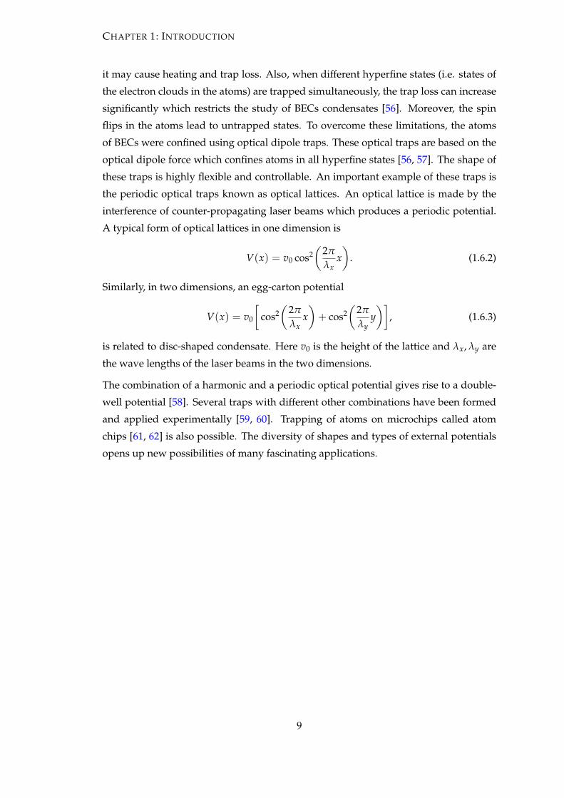
A typical form of optical lattices in one dimension is
V(x) = v0 cos2(
2π
λxx)
. (1.6.2)
Similarly, in two dimensions, an egg-carton potential
V(x) = v0
[cos2
(2π
λxx)+ cos2
(2π
λyy)]
, (1.6.3)
is related to disc-shaped condensate. Here v0 is the height of the lattice and λx, λy are
the wave lengths of the laser beams in the two dimensions.
The combination of a harmonic and a periodic optical potential gives rise to a double-
well potential [58]. Several traps with different other combinations have been formed
and applied experimentally [59, 60]. Trapping of atoms on microchips called atom
chips [61, 62] is also possible. The diversity of shapes and types of external potentials
opens up new possibilities of many fascinating applications.
9

CHAPTER 2
Mathematical Background
In the previous chapter we provided the basic information about solitons and the
physics of BECs along with their potential applications. In this chapter we will use a
variational approach to derive the Gross-Pitaevskii equation that describes the dynam-
ics of BECs. We will present the ground state properties of BECs. The basic nonlinear
solutions such as bright and dark solitons that exist in one dimensional Gross-Pitavskii
equation will be considered and their stability analysis will be presented.
2.1 The variational approximations
One of the most commonly used mathematical techniques in the study of BECs and
nonlinear optics is the variational approximation. This technique has been employed
to approximate solutions in various cases, particularly in the cases where solutions do
not exist in an analytical form. This method reduces a system having infinitely many
degrees of freedom to a finite-dimensional one. The objective of this method is to re-
duce a system with complex dynamics characterized by partial differential equations to
a relatively simple system of a few ordinary differential equations. It is a semi-analytic
method which is well known and has long been used to approximate solutions of non-
linear evolution equations. It is called semi-analytic because in practice this method
involves equations which may be too complicated to solve analytically and hence need
some numerical techniques for their solutions.
The method of the variational approximation can be systematically described in the
following steps [63]:
1. Find the Lagrangian or the Hamiltonian of the governing equations.
2. Select a suitable and mathematically tractable trial function (ansatz) that contains
10

CHAPTER 2: MATHEMATICAL BACKGROUND
a finite number of parameters called variational parameters. Typically, these pa-
rameters are the amplitude, width, phase, etc. of the wavefunction. These pa-
rameters are allowed to be functions of spatial and temporal variables.
3. Substitute the chosen ansatz into the Lagrangian and find the resulting sums (for
discrete systems) or integrations (for continuous systems).
4. Derive the Euler-Lagrange equations which lead to ordinary differential equa-
tions for the variational parameters. These equations can be solved either analyt-
ically or numerically to understand the dynamics of the system. It is important to
mention that there is no direct formal relationship between the governing equa-
tions and the system of Euler Lagrange equations [64].
There are several factors involved for the successful implementation of the variational
method. Mainly, this method depends on the ansatz representing the shape of the
wavefunction but the ansatz should be such that the resulting sums or integration can
be expressed in a closed form. Moreover, the number of variational parameters rep-
resenting the nature of the system also affects the accuracy of the method. A more
accurate approximation can be achieved at the cost of introducing more parameters in
the ansatz. However, the complexity of the calculations, of course, increases by adding
more parameters.
The applicability of a particular variational ansatz can be tested by comparison of the
results with direct numerical simulations of the given evolution equations. The com-
parison of the direct numerical simulation is really essential for the study of the stability
of the solution because this method sometimes shows a false instability of the solution
which is actually stable [64]. However, for the validity of the results, it is sufficient to do
the comparison at a few distinct values of the variational parameters. The approxima-
tions are considered to be reliable in wide parametric domains if at several benchmark
points they are sufficiently close to the results obtained through numerical simulations.
In the following, we employ the variational approach to derive the famous Gross-
Pitaevskii equation that describes the dynamics of BECs.
2.2 The Gross-Pitaevskii equation
We discuss a simple approach to describe a pure BEC taking into account the atom-
atom interactions in a mean-field approach (i.e. considering a many-body problem as
an effective one-body problem). Although the nature of the gases is very dilute in a
11

CHAPTER 2: MATHEMATICAL BACKGROUND
real condensate, atom-atom interactions cannot be neglected. In fact, the BEC in the
harmonic trap significantly increases the effects of the atom-atom interaction.
Let us consider a system of N number of spinless bosons described by spatial coordi-
nates rn. The starting point is the N-body Hamiltonian
H =N
∑n=1
(p2
n2m
+ V(rn)
)+
12
N
∑n=1
N
∑i =n
W(rn − ri). (2.2.1)
The first term herein represents the kinetic energy in which p is the momentum, V cor-
responds to the external trapping potential and W is the two-body interaction potential.
We use the Hartree approximation for seeking the ground state of the many-body sys-
tem. The physical idea of this approximation is that each boson feels the same mean-
field potential due to all the other bosons and the many-body wave function can be
approximated as a product of identical single-boson wave functions. For the N-body
system, we take the ansatz
uN(r1, r2, ..., rN , t) = ϕ(r1, t)ϕ(r2, t)...ϕ(rN , t), (2.2.2)
where ϕ denotes the wave function of the single-particle normalized to unity, that is
to be determined. This approximation assumes that all atoms occupy the same macro-
scopic state which is correct only for simple BECs. A more rigorous approach with a
time-dependent macroscopic number of particles in the condensate has been consid-
ered in [65]. Much more complicated cases, with more than one state with a macro-
scopic number of particles, called fragmented BECs, are also possible.
The collisional properties of particles in a dilute ultracold gas at low energies are de-
scribed by the s-wave scattering length and expressed in terms of one parameter − the
scattering length denoted by a [66]. The value of atomic scattering length can be either
positive or negative depending on the BEC species. The positive and negative values
correspond to repulsive and attractive interactions respectively between the atoms of
BEC. For example, the BEC formed by atomic vapors of sodium is repulsive and for
lithium is attractive. Once the atomic scattering length has been calculated or deter-
mined experimentally, one can use the fact that the two potentials having the same
scattering length exhibit the same properties in a system of dilute cold gas. Hence, the
interatomic interaction potential can replaced by an effective delta-function interaction
potential, i.e. W(rj − ri) = gδ(rj − ri), where g = 4πh2a/m, in which a represents the
scattering length and m is the mass of the particle.
Since pn = −ih∇n, the Hamiltonian for N interacting particles in the presence of trap-
ping potential V can be written as
H =N
∑n=1
(−h2
2m∇2
n + V(rn)
)+
g2
N
∑n=1
N
∑i =n
δ(rn − ri), (2.2.3)
12

CHAPTER 2: MATHEMATICAL BACKGROUND
where ∇n is the gradient relative to rn. The total Lagrangian associated with the Hamil-
tonian can then be written as
L =∫ ∞
−∞
N
∏k=1
drk
[ih2(u∗
N∂uN
∂t− uN
∂u∗N
∂t)−
N
∑n=1
(h2
2m|∇nuN |2 + V(rn)|uN |2
+g2
N
∑i =n
δ(rn − ri)|uN |2)]
, (2.2.4)
where the asterisk denotes the complex conjugation. Substituting the Hartree ansatz
(2.2.2) in the above expression of Lagrangian, we obtain several terms. Using the nota-
tion ϕ(rn, t) = ϕn, the first term is
∫ ∞
−∞
N
∏k=1
drkih2
u∗N
∂uN
∂t=
ih2
∫ ∞
−∞
N
∏k=1
drk
( N
∏i=1
ϕ∗i
)( N
∑l=1
∂ϕl
∂t
N
∏k =l
ϕk
)
=ih2
N
∑l=1
( ∫ ∞
−∞drlϕ
∗l
∂ϕl
∂t
)[ N
∏k =l
∫ ∞
−∞drkϕ∗
k ϕk
]=
ih2
N∫ ∞
−∞drϕ∗(r, t)
∂ϕ(r, t)∂t
. (2.2.5)
Here, the expression within square brackets above is equal to unity since ϕ has been
normalized.
The second term is the complex conjugate of the first term. i.e.
∫ ∞
−∞
N
∏k=1
drkih2
uN∂u∗
N∂t
=ih2
N∫ ∞
−∞drϕ(r, t)
∂ϕ∗(r, t)∂t
. (2.2.6)
The third term is
h2
2m
∫ ∞
−∞
N
∏k=1
drk
N
∑n=1
|∇nuN |2 =h2
2m
N
∑n=1
( ∫ ∞
−∞drn|∇nϕ(ri, t)|2
)( N
∏k =n
∫ ∞
−∞drkϕ∗
k ϕk
)
=h2
2mN∫ ∞
−∞dr|∇ϕ(r, t)|2. (2.2.7)
The fourth term leads to∫ ∞
−∞
N
∏k=1
drk
N
∑n=1
V(rn)|uN |2 = N∫ ∞
−∞drV(r)|ϕ(r, t)|2. (2.2.8)
Finally, the interaction term is
∫ ∞
−∞
N
∏k=1
drk
N
∑n=1
N
∑i =n
δ(rn − ri)|uN |2 = N(N − 1)∫ ∞
−∞dr|ϕ(r, t)|4. (2.2.9)
Substituting all these values in Eq. (2.2.4), we obtain
13

CHAPTER 2: MATHEMATICAL BACKGROUND
L = N∫ ∞
−∞dr[
ih2(ϕ∗ ∂ϕ
∂t− ϕ
∂ϕ∗
∂t)− h2
2m|∇ϕ|2 − V(r)|ϕ(r, t)|2 − g
2(N − 1)|ϕ(r, t)|4
].
(2.2.10)
The stationarity condition with respect to ϕ∗ is
δLδϕ∗ = 0, (2.2.11)
i.e.
N[
ih∂ϕ
∂t+
h2
2m∇2ϕ(r, t)− V(r)ϕ(r, t)− g(N − 1)|ϕ(r, t)|2ϕ(r, t)
]= 0. (2.2.12)
Hence, we obtain
ih∂ϕ(r, t)
∂t=
[− h2
2m∇2 + V(r) + g(N − 1)|ϕ(r, t)|2
]ϕ(r, t). (2.2.13)
The factor (N − 1) in the last term on the right hand side ensures that the interaction
term will vanish when N = 1. Nonetheless, in actual BECs the number of atom N is
at least 105. So we can replace the factor (N − 1) by N. The equation describing the
dynamics evolution of the BECs can then be written as
ih∂ϕ(r, t)
∂t=
[− h2
2m∇2 + V(r) + gN|ϕ(r, t)|2
]ϕ(r, t). (2.2.14)
We use scaling ψ(r, t) =√
Nϕ(r, t) to write the equation in its conventional form which
is
ih∂ψ(r, t)
∂t=
[− h2
2m∇2 + V(r) + g|ψ(r, t)|2
]ψ(r, t). (2.2.15)
This nonlinear equation was derived by Gross and Pitaevskii independently in 1961.
The Eq. (2.2.15) is called the time-dependent Gross-Pitaevskii (GP) equation also known
as the time-dependent nonlinear Schrödinger equation and is used to describe the
ground state as well as the excitations of the BEC. The predictions that arise from this
equation are in excellent agreement with experiments dealing with a quasi-pure con-
densate. The complex function ψ(r, t) in GP Eq. (2.2.15) is generally called the macro-
scopic wave function that characterizes the static and dynamic behavior of the conden-
sate. This function can be expressed in terms of density ρ(r, t) = |ψ(r, t)|2 and phase
θ(r, t) of the condensate as ψ(r, t) =√
ρeiθt. The GP model owns two integrals of mo-
tion which represent respectively the total number of atoms N and the energy of the
system E and are given as
N =∫ ∞
−∞|ψ(r, t)|2dr, (2.2.16)
14
CHAPTER 2: MATHEMATICAL BACKGROUND
E =∫ ∞
−∞
[h2
2m|∇ψ|2 + V|ψ|2 + 1
2g|ψ|4
]dr, (2.2.17)
where the first term represents the kinetic energy while the second and third terms
correspond to the potential energy and the interaction potential, respectively.
2.3 Ground state and Thomas-Fermi approximation
The ground state of Eq. (2.2.15) can be easily obtained by expressing the condensate
wave function ψ(r, t) = ψ0(r)e−iρ0t/h, where ψ0 is a function normalized to the number
of atoms N =∫|ψ0|2dr and ρ0 = ∂E
∂N is the chemical potential. Substitution of the above
expression into Eq. (2.2.15) gives the following time-independent form[− h2
2m∇2 + V(r) + g|ψ0(r)|2 − ρ0
]ψ0(r) = 0. (2.3.1)
When there is no interaction between the atoms of the condensates, i.e. g = 0, the
above equation reduces to the usual Schrödinger equation with the potential V. The
ground state (or the minimum energy state) in the presence of a harmonic trap can be
obtained by assuming that all bosons are in the lowest single body state. In this state,
the ground state solution ψ0 is the Gaussian function and is given as
ψ0 =√
N(
mΩgm
πh
)3/4
exp[−m2h
(Ωxx2 + Ωyy2 + Ωzz2)
], (2.3.2)
where Ωgm is the geometric mean of the confining frequencies, i.e. Ωgm = (ΩxΩyΩz)1/3.
For the attractive interatomic interaction, i.e. g < 0, the density of the atoms at the
centre of the trap increases while the kinetic energy tends to stabilize this increase.
Nevertheless, if the number of atoms N goes beyond a critical number Ncr, i.e. N > Ncr,
the central density and hence the rate of collisions grows to some such extent that the
kinetic energy could not balance this increase. Due to these strong collisions, atoms are
ejected out from the condensate in an energetic explosion resulting in the collapse of
the system. Experimental observations of collapse in the cases of attractive lithium and
rubidium were carried out in [67] and [68], respectively.
When the interaction between the atoms of the condensate is repulsive, i.e. g > 0, and
the number of atoms is reasonably large satisfying the condition Na/aho ≫ 1, where
aho =√
hmΩgm
, the atoms are pushed towards the boundaries of the condensate. Conse-
quently, the density at the centre tends to become flat with slow spatial variation and
the radius of condensate increases and is shown is Fig. 2.1 which has been taken from
[69]. Then the kinetic energy becomes very small as compared with the interaction and
15

CHAPTER 2: MATHEMATICAL BACKGROUND
Figure 2.1: Numerically obtained solutions (solid) of the stationary GP Eq. (2.3.1) in
a spherical trap with repulsive interatomic interaction corresponding toNaaho
= 1, 10, 100. The dashed curve represents the prediction for the ideal
gas. Figure has taken from [69].
potential energies and is significant only near the boundaries. If we neglect completely
the kinetic energy term in Eq. (2.3.1), the expression for the ground state density profile
of the system is
ρ(r) = |ψ0(r)|2 =ρ0 − V(r)
g, (2.3.3)
in the region where ρ0 > V(r) and ρ = 0 otherwise. This is known as the Thomas-
Fermi approximation [69] and is shown in Fig. 2.2.
2.4 Dimensionality reduction in GP models
The three dimensional GP Eq. (2.2.15) can be reduced to an effectively one dimensional
equation [70] by assuming the transverse confinement of the condensate tight enough,
16
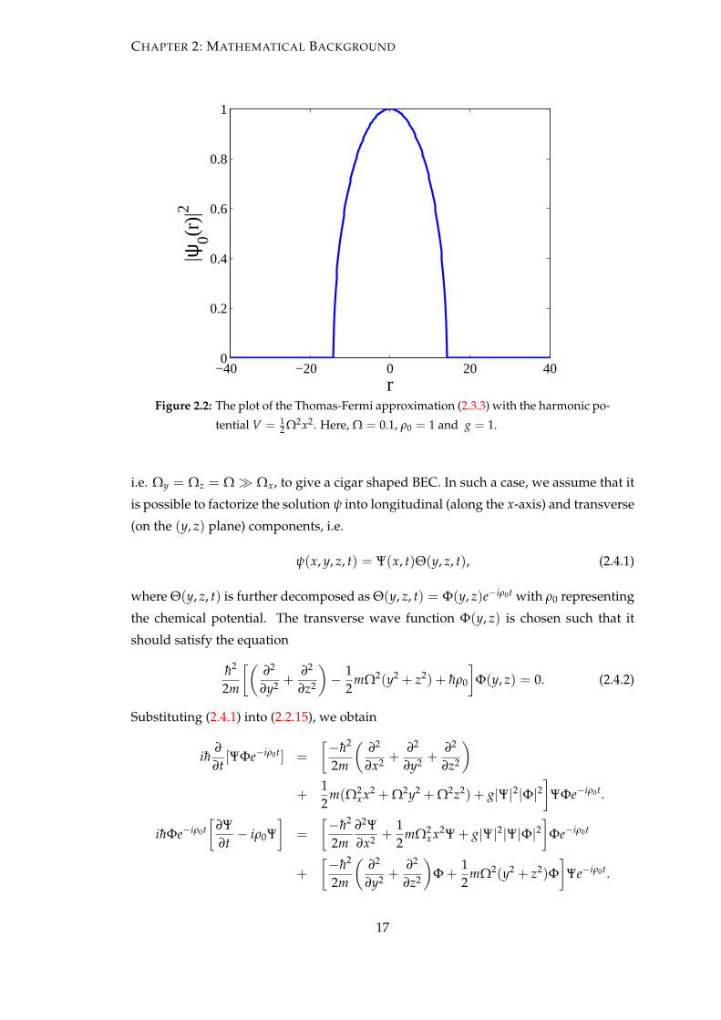
CHAPTER 2: MATHEMATICAL BACKGROUND
−40 −20 0 20 400
0.2
0.4
0.6
0.8
1
r
|ψ0(r
)|2
Figure 2.2: The plot of the Thomas-Fermi approximation (2.3.3) with the harmonic po-
tential V = 12 Ω2x2. Here, Ω = 0.1, ρ0 = 1 and g = 1.
i.e. Ωy = Ωz = Ω ≫ Ωx, to give a cigar shaped BEC. In such a case, we assume that it
is possible to factorize the solution ψ into longitudinal (along the x-axis) and transverse
(on the (y, z) plane) components, i.e.
ψ(x, y, z, t) = Ψ(x, t)Θ(y, z, t), (2.4.1)
where Θ(y, z, t) is further decomposed as Θ(y, z, t) = Φ(y, z)e−iρ0t with ρ0 representing
the chemical potential. The transverse wave function Φ(y, z) is chosen such that it
should satisfy the equation
h2
2m
[(∂2
∂y2 +∂2
∂z2
)− 1
2mΩ2(y2 + z2) + hρ0
]Φ(y, z) = 0. (2.4.2)
Substituting (2.4.1) into (2.2.15), we obtain
ih∂
∂t[ΨΦe−iρ0t] =
[−h2
2m
(∂2
∂x2 +∂2
∂y2 +∂2
∂z2
)+
12
m(Ω2xx2 + Ω2y2 + Ω2z2) + g|Ψ|2|Φ|2
]ΨΦe−iρ0t.
ihΦe−iρ0t[
∂Ψ∂t
− iρ0Ψ]
=
[−h2
2m∂2Ψ∂x2 +
12
mΩ2xx2Ψ + g|Ψ|2|Ψ|Φ|2
]Φe−iρ0t
+
[−h2
2m
(∂2
∂y2 +∂2
∂z2
)Φ +
12
mΩ2(y2 + z2)Φ]
Ψe−iρ0t.
17
CHAPTER 2: MATHEMATICAL BACKGROUND
Cancelation of e−iρ0t on both sides and rearranging the terms gives[h2
2m
(∂2
∂y2 +∂2
∂z2
)− 1
2mΩ2(y2 + z2) + hρ0
]ΦΨ + ihΦ
∂Ψ∂t
=
[−h2
2m∂2Ψ∂x2 +
12
mΩ2xx2Ψ
+g|Ψ|2Ψ|Φ|2]
Φ.
Using (2.4.2), the first term on the left hand side vanishes and we obtain
ihΦ∂Ψ∂t
=
[−h2
2m∂2Ψ∂x2 +
12
mΩ2xx2Ψ + g|Ψ|2Ψ|Φ|2
]Φ.
Multiplying both sides by Φ∗ and taking the double integral with respect to y and z
from −∞ to ∞ by letting∫ ∞−∞
∫ ∞−∞ |Φ(y, z)|2dydz = C1 and
∫ ∞−∞
∫ ∞−∞ |Φ(y, z)|4dydz =
C2, we get
ihC1∂Ψ∂t
=−h2
2mC1
∂2Ψ∂x2 +
12
C1mΩ2xx2Ψ + gC2|Ψ|2Ψ.
Finally, dividing throughout by C1 and setting gC2C1
= g1 yields
ih∂
∂tΨ(x, t) =
−h2
2m∂2
∂x2 Ψ(x, t) + V(x)Ψ(x, t) + g1|Ψ(x, t)|2Ψ(x, t), (2.4.3)
with V(x) = 12 mΩ2
xx2. Similarly, one can reduce (2.2.15) into a two dimensional GP
equation by assuming that the condensate is disc shaped. In that case, Eq. (2.2.15)
takes the following form
ih∂
∂tΨ(x, y, t) =
−h2
2m
(∂2
∂x2 +∂2
∂y2
)Ψ(x, y, t)+V(x, y)Ψ(x, y, t)+ g2|Ψ(x, y, t)|2Ψ(x, y, t),
(2.4.4)
where V(x, y) = 12 mΩ2(x2 + y2).
2.5 Dimensionless form of GP equation
One can reduce Eq. (2.4.3) to dimensionless form. To do so, we substitute Ψ = αu,
t = βt, x = γx, where α, β and γ are real constants, in Eq. (2.4.3) to obtain
ihα
βut = − h2α
2mγ2 uxx +12
αγ2Ω2 x2u + g1α3|u|2u.
Multiplying throughout by β/hα, we obtain
iut = − hβ
2mγ2 uxx +βγ2Ω2
2hx2u +
g1α2β
h|u|2u.
When g1 > 0, say g1 = g, we set
hβ
mγ2 = 1,βγ2
h= 1,
gα2β
h= 1.
18

CHAPTER 2: MATHEMATICAL BACKGROUND
These equations yield
β = m1/2, γ = h1/2m−1/4, α = g−1/2h1/2m−1/4.
For g1 < 0, say g1 = −g, we use the same settings as above. Finally, we omit tilde to
obtain the following dimensionless form of the one-dimensional GP equation
iut = −12
uxx + Vu ± |u|2u, (2.5.1)
where subscripts denote the partial derivatives.
When the condensate is homogeneous, i.e. V = 0, Eq. (2.5.1) reduces to
iut = −12
uxx ± |u|2u, (2.5.2)
The homogeneous Eq. (2.5.2) is completely integrable [3, 71] and has an infinite number
of integrals of motion. The most fundamental ones which have clear meanings are the
number of particles N, the momentum P and the energy E, which are respectively
given as
N =∫ ∞
−∞|u|2dx, (2.5.3)
P =i2
∫ ∞
−∞(uu∗
x − u∗ux)dx, (2.5.4)
E =12
∫ ∞
−∞(|ux|2 + |u|4)dx. (2.5.5)
These quantities remain conserved as the systems described by Eq. (2.5.2) are conser-
vative.
2.6 Solutions of one-dimensional GP equations and their sta-
bility
The homogeneous one-dimensional GP Eq. (2.5.2) possess an infinite number of solu-
tions. The well-known solutions are the plane-wave solution, the dark solitons and the
bright solitons. In the following, we will present the basic information and the stability
analysis of these solutions.
2.6.1 The plane-wave solution
The simplest nontrivial solution of Eq. (2.5.2) is the plane-wave solution given by
u(x, t) =√
ρ0 exp[i(κx − ωt)], (2.6.1)
19

CHAPTER 2: MATHEMATICAL BACKGROUND
where κ, ω and ρ0, represent respectively the wave number, frequency and square of
the amplitude of the plane-wave. A relationship between the wave number and fre-
quency can be obtained by introducing this solution into Eq. (2.5.2), which yields
ω =12
κ2 ± ρ0. (2.6.2)
The above expression describing the plane-wave solution is known as the dispersion
relation. Differentiating Eq. (2.6.2) partially with respect to κ gives the group velocity v
of the plane wave solution, i.e. v = ∂ω∂κ = κ. Since |u|2 represents the density, when the
density is small, the plane-wave solution satisfies the linear GP equation iut +12 uxx = 0,
with the dispersion relation ω = 12 κ2. If the system is confined to a length L, the
integrals of motion for the plane-wave solution have the following values,
N = ρ0L, P = κρ0L = κN, E =12[ρ0L(κ2 + ρ0)] =
12
[P2
N+
N2
L
]. (2.6.3)
These equations show that the plane-wave solution behaves as a classical particle with
the effective mass Mpws, momentum Ppws and energy Epws given by
Mpws = ρ0L, Ppws = Mpwsv, Epws =12
Mpwsv2 +M2
pws
2L.
One can differentiate energy Epws and momentum Ppws partially with respect to velocity
v = κ to obtain a standard equation of classical mechanics
∂Epws
∂Ppws= v,
which justifies the particle-like nature of the plane-wave solution.
Let us now discuss the stability of the plane wave solution given by Eq. (2.6.1) in the
defocusing NLS equation
iut = −12
uxx + |u|2u, (2.6.4)
We add a small perturbation to the plane wave solution, i.e.
u(x, t) =√
ρ0 exp[i(κx − ωt)] + ϵ f (x, t), (2.6.5)
where f is any complex valued function and ϵ ≪ 1 is a perturbation parameter. Differ-
entiating Eq. (2.6.5) partially with respect to t and x, we obtain
ut = −iω√
ρ0 exp[i(κx − ωt)] + ϵ ft,
uxx = −κ2√ρ0 exp[i(κx − ωt)] + ϵ fxx.
Substituting these values into Eq. (2.6.4) and retaining the terms linear in ϵ gives(ω− κ2
2− ρ0
)√
ρ0 exp[i(κx−ωt)]+ ϵ
[i ft +
12
fxx − 2ρ0 f − ρ0 f ∗ exp (2iκx − 2iωt)]= 0.
20

CHAPTER 2: MATHEMATICAL BACKGROUND
Using the dispersion relation, the first term above will vanish and we are left with
i ft +12
fxx − 2ρ0 f − ρ0 f ∗ exp (2iκx − 2iωt) = 0.
We substitute f (x, t) = F(x, t) exp[i(κx − ωt)] (where F is any complex valued func-
tion) in the above equation to obtain
iFt +12
Fxx + iκFx − ρ0(F + F∗) = 0.
Next, suppose that F(x, t) = α(x) exp (iqt) + iβ∗(x) exp (−iqt), where α and β are com-
plex valued functions and q is a real number. Inserting this expression of F into the last
equation and equating to zero the coefficients of exp (iqt) and exp (−iqt), we obtain
12
αxx + iκαx − (q + ρ0)α − ρ0β = 0,
12
βxx − iκβx + (q − ρ0)β − ρ0α = 0.
Since the above coupled equations are linear in α and β, one can substitute
α = α0 exp (−ipx) and β = β0 exp (−ipx) to obtain the following linear algebraic equa-
tions
(q − κp + ρ0 + p2/2)α0 + ρ0β0 = 0, (2.6.6)
−ρ0α0 + (q − κp − ρ0 − p2/2)β0 = 0. (2.6.7)
The system of Eq. (2.6.6) and Eq. (2.6.7) is homogeneous and can be expressed in the
matrix form AX = b with the coefficient matrix A given as
A =
[q − κp + ρ0 + p2/2 ρ0
−ρ0 q − κp − ρ0 − p2/2
].
The system will have a non-trivial solution if det(A) = 0. This implies that
(q − κp)2 = p2(
p2
4+ ρ0
), (2.6.8)
or
q = κp ±
√p2
(p2
4+ ρ0
). (2.6.9)
Eq. (2.6.9) shows that the value of q will remain real for any given real value of p.
Hence,
f (x, t) = F(x, t) exp[i(κx − ωt)] = [α(x) exp (iqt) + iβ∗(x) exp (−iqt)] exp[i(κx − ωt)]
= α0 exp[i(κ − p)x + i(q − ω)t]
+ β0 exp[i(κ − p)x − i(q + ω)t].
21

CHAPTER 2: MATHEMATICAL BACKGROUND
The above expression shows that f will not grow for any real values of p and q which
in turn implies that the small excitations of the plane wave solution of the defocus-
ing NLS equation will be stable. One can find the minimum group velocity of these
small excitations for κ = 0. Differentiating Eq. (2.6.8) with respect to p gives the group
velocity of the excitation which is denoted by vg, i.e.
vg =dqdp
=2ρ0 + p2√
4ρo + p2. (2.6.10)
Now, we differentiate vg twice with respect to p and equate the first derivative of vg to
zero. The critical value we obtain is p = 0 and the second derivative of vg is positive at
this value of p, indicating that p = 0 is the point of minimum value. We plug p = 0 in
Eq. (2.6.10) to get the minimum value of the group velocity which is (vg)min =√
ρ0.
Let us now consider the stability of the plane wave solution in the focusing NLS equa-
tion
iut = −12
uxx − |u|2u. (2.6.11)
It is easy to see that if we follow a similar procedure as before, the following relation
between p and q is obtained
q = κp ±
√p2
(p2
4− ρ0
). (2.6.12)
This shows that q will be complex for p2 < 4ρ0. Consequently, f will grow exponen-
tially and hence the plane wave solution will become unstable.
2.6.2 Matter wave dark solitons
Let us now take into account the case of repulsive interatomic interaction in the con-
densate. In this case the sign of the nonlinear term in Eq. (2.5.2) should be positive
and the resulting GP equation possesses a dark soliton solution. This solution can be
considered as the nonlinear excitation of the plane-wave solution. The general form of
the dark soliton solution is [71]
u(x, t) =√
ρ0[A tanh η + iB] exp[i(κx − ωt)], (2.6.13)
where η =√
ρ0 A(x −√ρ0x0) and the parameters A, B, x0 are in general functions of
time t. The parameter A determines the depth√
ρ0 A of the dark soliton, while the
parameter x0 represents the soliton centre and is given by x0 = xi + vt. Here xi is
an arbitrary real number which denotes the initial location of the dark soliton. The fre-
quency ω of the dark soliton is given by the dispersion relation (2.6.2) (with the positive
22

CHAPTER 2: MATHEMATICAL BACKGROUND
−10 −5 0 5 100
0.2
0.4
0.6
0.8
1
x
|u|2
Figure 2.3: Plot of a black soliton (black) with parameter values A = 1, B = v = 0 and
a grey soliton (blue) with A =√
32 , B = v = 0.5.
sign) of the background solution. To obtain the relationships between the parameters
of the dark soliton, we differentiate the solution (2.6.13) partially with respect to t and
x to yield
ut =
(Bω
√ρ0 − ρ0vA2sech2η − iAω
√ρ0 tanh η
)exp[i(κx − ωt)],
uxx =
(− κ2A
√ρ0 tanh η + 2iκA2ρ0sech2η − iκ2B
√ρ0
)exp[i(κx − ωt)].
Here, we have assumed that the initial location of the dark soliton is at the origin.
Substituting the above expressions of u, ut and uxx in Eq. (2.5.2) (with positive sign)
and equating to zero the real and imaginary parts, we find that the parameters A, B
and v are related through the equations A2 + B2 = 1 and κ + (B − v)√
ρ0 = 0. In the
case of B = v = 0, the dark soliton becomes a stationary kink also called a black soliton
and has unit depth. The dark soliton moving with some non-zero velocity is also called
a grey soliton. In particular, for B = v = ±1, the depth of the solution vanishes and
the dark soliton becomes the background solution. The profiles of the black and grey
solitons are shown in Fig. 2.3.
When the background solution is at rest, i.e. κ = 0, we have B = v. Then the minimum
value ρmin of the dark soliton can be obtained by differentiating |u|2 partially with
respect to x and equating it to zero, i.e.
∂|u|2∂x
= 0. (2.6.14)
23

CHAPTER 2: MATHEMATICAL BACKGROUND
Here,
|u|2 = ρ0[A2 tanh2 η + B2]. (2.6.15)
Using Eq. (2.6.14), the critical point we obtain is x =√
ρ0x0. Substituting this value
back in Eq. (2.6.15) yields
ρmin = ρ0B2 = ρ0v2. (2.6.16)
Sometimes, it is convenient to parameterize A and B as A = cos ϕ and B = sin ϕ, where
ϕ is called the soliton phase angle. In the limiting case when x → ±∞, the dark soliton
coincides with the plane-wave solution. However, the plane waves are shifted in phase
at the different edges. The total phase jump ∆ϕ across the dark soliton is given by
∆ϕ = 2[
arctan(
BA
)− π
2
]= −2 arctan
(AB
). (2.6.17)
We now consider the integrals of motion for dark soliton. Since the integrals of mo-
tion (2.5.3-2.5.5) describe both the background and the dark soliton, they have been
modified [7] to extract the corresponding contribution of the background. After such a
modification, the integrals of motion for the dark soliton become finite. The renormal-
ized integrals of motion for the dark soliton are
Nds =∫ ∞
−∞(ρ0 − |u|2)dx, (2.6.18)
Pds =i2
∫ ∞
−∞(uu∗
x − u∗ux)
(1 − ρ0
|u|2
)dx, (2.6.19)
Eds =12
∫ ∞
−∞
[|ux|2 + (|u|2 − ρ0)
2]
dx, (2.6.20)
where Nds, Pds and Eds represent respectively the number of atoms, momentum and
energy of the dark soliton. We evaluate these integrals of motion in the simpler case
when the background is static, i.e. κ = 0. Substituting the soliton solution (2.6.13) into
the above integrals, we find
Nds = 2A√
ρ0, Pds = −2vρ0
√1 − v2 + 2ρ0 arctan
(√1 − v2
v
), Eds =
43
ρ03/2(1− v2)3/2.
(2.6.21)
Differentiating the momentum and energy of the dark soliton with respect to velocity,
we obtaindPds
dv= −4c2
s
√1 − v2, (2.6.22)
dEds
dv= −4c2
s v√
1 − v2. (2.6.23)
24

CHAPTER 2: MATHEMATICAL BACKGROUND
Using chain rule, we find the following simple relation
dEds
dPds= v, (2.6.24)
which clearly indicates that the dark soliton behaves as a classical particle. Since the left
hand side of Eq. (2.6.22) represents the mass, an effective mass mds can be incorporated
to the dark soliton as mds = −4ρ0 A. This shows that the dark soliton is described by a
negative effective mass.
2.6.2.1 The stability of dark solitons
Several methods have been used to study the dynamics of matter wave dark solitons
in a quasi one dimensional GP equation. Physicists first thought that dark solitons
are stable solutions. Kivshar and Krolikowski were the first who used a variational
approach and determined a criterion for the stability of dark solitons [72]. However,
the existence and stability of dark solitons in a generalized model of GP equation were
recently studied rigorously in [73, 74]. The persistence and stability of dark solitons in
the absence of external potential was considered in [73] while a more general model in
the presence of the potential was investigated in [74]. Here, we will discuss the linear
stability of dark solitons numerically in the absence and presence of a harmonic trap.
In order to discuss the linear stability of dark soliton, we set u = U exp(−it) into Eq.
(2.5.1) with defocusing nonlinearity to obtain
iUt = −12
Uxx + VU − U + |U|2U. (2.6.25)
We first find the dark soliton solution numerically in the absence of the magnetic trap,
i.e. V = 0, and Eq. (2.6.25) reduces to
iUt = −12
Uxx − U + |U|2U. (2.6.26)
Let us assume Ut = 0, so that we are considering the black soliton described in the
previous section. Discretizing the resulting equation, we obtain
Un+1 − 2Un + Un−1
2∆x2 − |Un|2Un + Un = 0, for n = 1, 2, ..., N. (2.6.27)
Eq. (2.6.27) represents a system of nonlinear algebraic equations. We solve this system
by using Newton’s method with Neumann boundary conditions U0 = U1, UN+1 =
UN through the MATLAB built-in function FSOLVE to obtain the dark soliton solution
numerically which is shown in Fig. 2.4. Note that Eq. (2.6.26) is invariant under the
transformation U → −U. This means that the negative dark soliton exists and can be
obtained similarly.
25
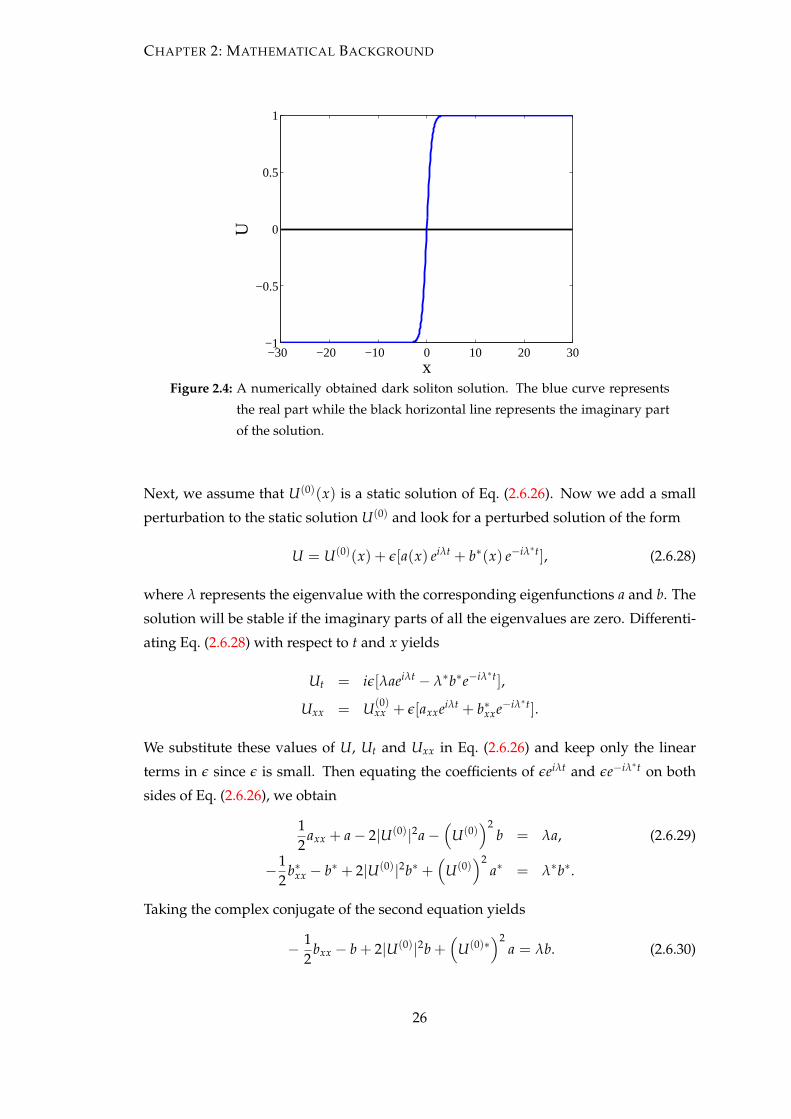
CHAPTER 2: MATHEMATICAL BACKGROUND
−30 −20 −10 0 10 20 30−1
−0.5
0
0.5
1
x
U
Figure 2.4: A numerically obtained dark soliton solution. The blue curve represents
the real part while the black horizontal line represents the imaginary part
of the solution.
Next, we assume that U(0)(x) is a static solution of Eq. (2.6.26). Now we add a small
perturbation to the static solution U(0) and look for a perturbed solution of the form
U = U(0)(x) + ϵ[a(x) eiλt + b∗(x) e−iλ∗t], (2.6.28)
where λ represents the eigenvalue with the corresponding eigenfunctions a and b. The
solution will be stable if the imaginary parts of all the eigenvalues are zero. Differenti-
ating Eq. (2.6.28) with respect to t and x yields
Ut = iϵ[λaeiλt − λ∗b∗e−iλ∗t],
Uxx = U(0)xx + ϵ[axxeiλt + b∗xxe−iλ∗t].
We substitute these values of U, Ut and Uxx in Eq. (2.6.26) and keep only the linear
terms in ϵ since ϵ is small. Then equating the coefficients of ϵeiλt and ϵe−iλ∗t on both
sides of Eq. (2.6.26), we obtain
12
axx + a − 2|U(0)|2a −(
U(0))2
b = λa, (2.6.29)
−12
b∗xx − b∗ + 2|U(0)|2b∗ +(
U(0))2
a∗ = λ∗b∗.
Taking the complex conjugate of the second equation yields
− 12
bxx − b + 2|U(0)|2b +(
U(0)∗)2
a = λb. (2.6.30)
26

CHAPTER 2: MATHEMATICAL BACKGROUND
The system of Eq. (2.6.29) and Eq. (2.6.30) represents a linear eigenvalue problem. Dis-
cretizing Eq. (2.6.29) and Eq. (2.6.30) gives
an+1 − 2an + an−1
2∆x2 + an − 2|U(0)n |2an −
(U(0)
n
)2bn = λan, (2.6.31)
−bn+1 − 2bn + bn−1
2∆x2 − bn + 2|U(0)n |2bn +
(U(0)∗
n
)2an = λbn, (2.6.32)
where n = 1, 2, ..., N. Using the Neumann boundary conditions a0 = a1, aN = aN+1,
b0 = b1, bN = bN+1, the above system of Eq. (2.6.31) and Eq. (2.6.32) can be written in a
matrix form as
AX = λX,
where
A =
[A1 D
−D∗ −A1
],
with
A1 =
a111
2∆x2 0 . . . 0
12∆x2 a22
12∆x2 . . . 0
0 12∆x2 a33 . . . 0
......
.... . .
...
0 0 0 . . . aNN
,
D =
−(
U(0)1
)20 . . . 0
0 −(
U(0)2
)2. . . 0
......
. . ....
0 0 . . . −(
u(0)N
)2
.
In the matrix A1 the entries of the principal diagonal are given by aii = 1 − 2|U(0)i |2 −
12∆x2 when i = 1, N and aii = 1 − 2|U(0)
i |2 − 1∆x2 when i = 2, 3, ..., N − 1.
We find the eigenvalues of the stability matrix A, which are depicted in Fig. 2.5. This
shows that all the eigenvalues are real except a pair of eigenvalues lying on the vertical
axis. The magnitude of this pair of eigenvalues is very small. As ∆x → 0, this pair
tends to zero so that all the eigenvalues become real, showing that the dark solution is
a stable solution. We also solve the time-dependent Eq. (2.6.26) using a Runge-Kutta
method of order four to confirm the stability of the solution as shown in Fig. 2.6.
27

CHAPTER 2: MATHEMATICAL BACKGROUND
−100 −50 0 50 100−3
−2
−1
0
1
2
3x 10
−7
Re(λ)
Im(λ
)
Figure 2.5: The structure of the eigenvalues in the complex plane for the solution
shown in Fig. 2.4.
x
t
−10 −5 0 5 10
50
100
150
200
250
300
350
400
0.2
0.4
0.6
0.8
1
Figure 2.6: Contour plot obtained through the direct numerical integration of Eq.
(2.6.26) depicting the time evolution of the dark soliton solution shown
in Fig. 2.4.
28

CHAPTER 2: MATHEMATICAL BACKGROUND
2.6.2.2 The stability of dark solitons in the inhomogeneous case
Let us now consider the inhomogeneous case with V = 12 Ω2x2. We follow the same
procedure as above and find numerically the dark soliton solution in the presence of
the magnetic trap. The profiles of the dark soliton for different values of the trapping
strength Ω are shown in Fig. 2.7. The profiles show that the width of the dark soliton
decreases with the increasing strength of the trap. One can also see that the solution
tends to zero due to the influence of the magnetic trap.
−40 −20 0 20 40−1
−0.5
0
0.5
1
x
u
(a)
−40 −20 0 20 40−1
−0.5
0
0.5
1
x
u
(b)
−40 −20 0 20 40−1
−0.5
0
0.5
1
x
u
(c)
−40 −20 0 20 40−1
−0.5
0
0.5
1
x
u
(d)
Figure 2.7: The profiles of a dark soliton in the presence of the magnetic trap with
trapping strength Ω = 0.05, 0.1, 0.15, 0.2 respectively. In each figure the
blue curve represents the real part while the black horizontal line repre-
sents the imaginary part of the solution. The higher the value of Ω, the
smaller the width of the dark soliton.
Starting from the static solution shown in Fig. 2.7 and adding a small perturbation to
29

CHAPTER 2: MATHEMATICAL BACKGROUND
−100 −50 0 50 100
−3
−2
−1
0
1
2
3
x 10−11
Re(λ)
Im(λ
)
Figure 2.8: The structure of the eigenvalues in the complex plane for the dark soliton
in the presence of the magnetic trap with Ω = 0.1.
it, the following stability equations are obtained
12
axx − Va + a − 2|U(0)|2a −(
U(0))2
b = λa, (2.6.33)
−12
bxx + Vb − b + 2|U(0)|2b +(
U(0)∗)2
a = λb. (2.6.34)
We discretize the above two equations and write the resulting system of equations in
a matrix form. Then we find the eigenvalues of the stability matrix and are shown in
Fig. 2.8. The figure shows that the dark soliton in the presence of the magnetic trap is
stable. The time evolution of the solution is shown in Fig. 2.9.
2.6.2.3 Travelling dark solitons
Because solitons of Eq. (2.6.26) are translationally invariant, we can study the existence
and stability of solitons in a moving coordinate frame. Therefore, we substitute ξ =
x − vt and τ = t (where v represents the velocity of the dark soliton) in Eq. (2.6.26),
then
Ut = −vUξ + Uτ, Uxx = Uξξ ,
and Eq. (2.6.26) takes the form
i(−vUξ + Uτ) +12
Uξξ + U − |U|2U = 0. (2.6.35)
The exact analytical solution independent of τ of Eq. (2.6.35) is given by
U(ξ) = A tanh(Aξ) + iv, A2 + v2 = 1. (2.6.36)
30

CHAPTER 2: MATHEMATICAL BACKGROUND
x
t
−40 −20 0 20 40
50
100
150
200
250
300
350
400
0.1
0.2
0.3
0.4
0.5
0.6
0.7
0.8
0.9
Figure 2.9: Contour plot obtained through the direct numerical integration of Eq.
(2.6.25) depicting the time evolution of the dark soliton solution shown
in Fig. 2.7.
To find this solution numerically we discretize Eq. (2.6.35) to obtain
− iv(
Un+1 − Un−1
2∆x
)+
Un+1 − 2Un + Un−1
2∆x2 + Un − |Un|2Un = 0, for n = 1, 2, ..., N.
(2.6.37)
Solving this above system of equations using Newton’s method with the Neumann
boundary conditions, we obtain numerically the travelling dark soliton solution in one
dimension having velocity v.
2.6.2.4 The stability of travelling dark soliton solution
Suppose that U(0) is a steady state solution of Eq. (2.6.35) and
U = U(0)(ξ) + ϵ[a(ξ) eiλτ + b∗(ξ) e−iλ∗τ], (2.6.38)
be the perturbed solution of Eq. (2.6.35), then we have
12
aξξ − ivaξ + a − 2|U(0)|2a −(
U(0))2
b = λa, (2.6.39)
−12
bξξ − ivbξ − b + 2|U(0)|2b +(
U(0)∗)2
a = λb. (2.6.40)
The system of Eq. (2.6.39) and Eq. (2.6.40) represents a linear eigenvalue problem. Dis-
cretizing these equations givesan+1 − 2an + an−1
2∆x2 − ivan+1 − an−1
2∆x+ an − 2|U(0)
n |2an −(
U(0)n
)2bn = λan, (2.6.41)
−bn+1 − 2bn + bn−1
2∆x2 − ivbn+1 − bn−1
2∆x− bn + 2|U(0)
n |2bn +(
U(0)∗n
)2an = λbn, (2.6.42)
31

CHAPTER 2: MATHEMATICAL BACKGROUND
where n = 1, 2, ..., N. We use the Neumann boundary conditions and write the above
system of equations (2.6.41) and (2.6.42) in a matrix form. After finding the eigenval-
ues of the stability matrix we conclude that the travelling dark soliton solution of one
dimensional NLS equation is stable for all the values of velocity v where it exists.
2.6.3 Matter wave bright solitons and their stability
The negative sign in Eq. (2.5.2) corresponds to the attractive interaction between the
atoms of BECs. In such a case, there exists a bright soliton solution of the following
form [3]
u(x, t) = Dsechθ exp[i(κx − ωt)], θ(x, t) = D(x − vt), (2.6.43)
and is shown in Fig. 2.11. Here, the parameter D denotes the amplitude of the bright
soliton. Differentiating Eq. (2.6.43) partially with respect to t and x, we get
ut = Dsechθ[Dv tanh θ − iω] exp[i(κx − ωt)],
uxx = Dsechθ(D2 − κ2 − 2D2sech2θ − 2iκD tanh θ) exp[i(κx − ωt)].
Substituting ut and uxx in Eq. (2.6.11) and equating the real and imaginary parts to zero,
the following relations are obtained
ω =12(κ2 − D2), v = κ.
To find the integrals of motion for the bright soliton, we insert Eq. (2.6.43) into Eqs.
(2.5.3-2.5.5), which yield
N = 2D, P = 2Dκ = Nκ, E = Dκ2 − 13
D3 =12
[2Dκ2 − 1
12(2D)3
]. (2.6.44)
It is easy to associate the concept of effective mass Mbs, momentum Pbs and energy Ebs
to the bright soliton through these equations by expressing them into the following
form
Mbs = 2D, Pbs = Mbsv, Ebs =12
Mbsv2 − 124
M3bs.
The right hand side in the energy equation is the sum of two terms, the kinetic energy
and the binding energy respectively of the quasi-particle associated with the bright so-
lion. Differentiating the above expressions for energy and momentum over the soliton
velocity v, we obtain∂Ebs
∂Pbs= v.
This equation shows that the bright soliton behaves as a classical particle like the dark
soliton.
32

CHAPTER 2: MATHEMATICAL BACKGROUND
x
t
−40 −20 0 20 40
50
100
150
200
250
300
350
400
0.2
0.4
0.6
0.8
1
1.2
1.4
Figure 2.10: Contour plot obtained through the direct numerical integration of Eq.
(2.6.11) depicting the time evolution of the bright soliton solution shown
in Fig. 2.11.
Next, we follow the same procedure as for the dark soliton to investigate the stability
of bright soliton. The eigenvalues of the stability matrix found in this case indicate that
the bright soliton is a stable solution. The time evolution of the solution is shown in
Fig. 2.10.
We also find the bright soliton solution in the presence of a magnetic trap. The presence
of the trap does not affect the solution significantly as the width of the bright soliton
is small as compared with the trapping strength Ω. The two bright soliton solutions,
one in the absence and other in the presence of the trap are shown in Fig. 2.11. Both
solutions are almost same. The solution in the presence of the trap is found to stable as
well.
2.7 Multi-component BECs and coupled system of Gross-Pitaevskii
equations
Gaseous BECs were first achieved in the clouds of atoms in a single spin state of the
ground state of rubidium [41], sodium [42] and lithium [75]. The diversity in the trap-
ping techniques for BECs made it possible to confine simultaneously the different hy-
perfine states of the condensate. The first such experiment was reported for mixtures of
two magnetically trapped hyperfine states of rubidium [76], in which similarities and
differences between the behaviours of the two spin states were studied. Simultaneous
33

CHAPTER 2: MATHEMATICAL BACKGROUND
−40 −20 0 20 400
0.2
0.4
0.6
0.8
1
1.2
1.4
1.6
x
u
Figure 2.11: Comparison between the untrapped (blue) and the trapped (black
dashed) bright solitons. For the trapped bright soliton, Ω = 0.2. Both
graphs are almost same showing that the magnetic trap does not affect
the stability of the solution.
confinement of BECs of sodium atoms in several hyperfine states using optical trap was
achieved in [56]. The optical trap allowed the confinement of atoms of sodium conden-
sate independent of their spin orientations and provided the opportunity of studying
the so called spinor condensates [77].
On the other hand, mixtures of two different species of condensates such as potassium-
rubidium (41K −87 Rb) [78] and lithium-cesium (7Li −133 Cs) [79] have been created ex-
perimentally. The mean field model describing the dynamics of such multi-component
condensates is a system of coupled GP equations. Typically, the two-mode representa-
tion of the GP system is derived below.
2.7.1 Two-mode representations of the GP equation
The dynamics of a dilute gas containing interacting bosons of the same species in the
context of mean field under the influence of a magnetic trap can be illustrated by the
GP equation which in the cartesian coordinate system can be given as
ih∂ψ
∂t=
[−h2
2m
(∂2
x + ∂2y + ∂2
z
)+ V(x, y, z)
]ψ + g|ψ|2ψ. (2.7.1)
Here V(x, y, z) = V1(x) + V2(y) + V3(z) is the external magnetic trap.
To obtain an accurate formulation, the two-mode representation of ψ along with the
34
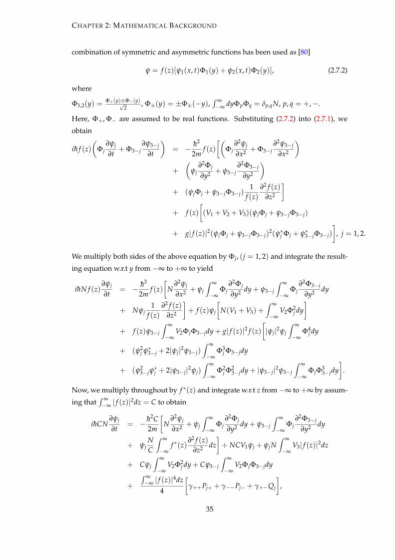
CHAPTER 2: MATHEMATICAL BACKGROUND
combination of symmetric and asymmetric functions has been used as [80]
ψ = f (z)[ψ1(x, t)Φ1(y) + ψ2(x, t)Φ2(y)], (2.7.2)
where
Φ1,2(y) =Φ+(y)±Φ−(y)√
2, Φ±(y) = ±Φ±(−y),
∫ ∞−∞ dyΦpΦq = δp,qN, p, q = +,−.
Here, Φ+, Φ− are assumed to be real functions. Substituting (2.7.2) into (2.7.1), we
obtain
ih f (z)(
Φj∂ψj
∂t+ Φ3−j
∂ψ3−j
∂t
)= − h2
2mf (z)
[(Φj
∂2ψj
∂x2 + Φ3−j∂2ψ3−j
∂x2
)+
(ψj
∂2Φj
∂y2 + ψ3−j∂2Φ3−j
∂y2
)+ (ψjΦj + ψ3−jΦ3−j)
1f (z)
∂2 f (z)∂z2
]+ f (z)
[(V1 + V2 + V3)(ψjΦj + ψ3−jΦ3−j)
+ g| f (z)|2(ψjΦj + ψ3−jΦ3−j)2(ψ∗
j Φj + ψ∗3−jΦ3−j)
], j = 1, 2.
We multiply both sides of the above equation by Φj, (j = 1, 2) and integrate the result-
ing equation w.r.t y from −∞ to +∞ to yield
ihN f (z)∂ψj
∂t= − h2
2mf (z)
[N
∂2ψj
∂x2 + ψj
∫ ∞
−∞Φj
∂2Φj
∂y2 dy + ψ3−j
∫ ∞
−∞Φj
∂2Φ3−j
∂y2 dy
+ Nψj1
f (z)∂2 f (z)
∂z2
]+ f (z)ψj
[N(V1 + V3) +
∫ ∞
−∞V2Φ2
j dy]
+ f (z)ψ3−j
∫ ∞
−∞V2ΦjΦ3−jdy + g| f (z)|2 f (z)
[|ψj|2ψj
∫ ∞
−∞Φ4
j dy
+ (ψ2j ψ∗
3−j + 2|ψj|2ψ3−j)∫ ∞
−∞Φ3
j Φ3−jdy
+ (ψ23−jψ
∗j + 2|ψ3−j|2ψj)
∫ ∞
−∞Φ2
j Φ23−jdy + |ψ3−j|2ψ3−j
∫ ∞
−∞ΦjΦ3
3−jdy]
.
Now, we multiply throughout by f ∗(z) and integrate w.r.t z from −∞ to +∞ by assum-
ing that∫ ∞−∞ | f (z)|2dz = C to obtain
ihCN∂ψj
∂t= − h2C
2m
[N
∂2ψj
∂x2 + ψj
∫ ∞
−∞Φj
∂2Φj
∂y2 dy + ψ3−j
∫ ∞
−∞Φj
∂2Φ3−j
∂y2 dy
+ ψjNC
∫ ∞
−∞f ∗(z)
∂2 f (z)∂z2 dz
]+ NCV1ψj + ψjN
∫ ∞
−∞V3| f (z)|2dz
+ Cψj
∫ ∞
−∞V2Φ2
j dy + Cψ3−j
∫ ∞
−∞V2ΦjΦ3−jdy
+
∫ ∞−∞ | f (z)|4dz
4
[γ++Pj+ + γ−−Pj− + γ+−Qj
],
35

CHAPTER 2: MATHEMATICAL BACKGROUND
where
Pj± = |ψj|2ψj ± (ψ2j ψ∗
3−j + 2|ψj|2ψ3−j) + (ψ23−jψ
∗j + 2|ψ3−j|2ψj)± |ψ3−j|2ψ3−j,
Qj = 6|ψj|2ψj − 4|ψ3−j|2ψj − 2ψ23−jψ
∗j ,
γpq = g∫ ∞
−∞Φ2
p(y)Φ2q(y)dy.
The last equation is equivalent to the following equation
ih∂ψj
∂t= − h2
2m
[∂2ψj
∂x2 + ψ3−j1N
∫ ∞
−∞Φj
∂2Φ3−j
∂y2 dy]+ V1ψj + ψ3−j
1N
∫ ∞
−∞V2ΦjΦ3−jdy
+
∫ ∞−∞ | f (z)|4dz
4NC
[γ++Pj+ + γ−−Pj− + γ+−Qj
].
Finally, multiplying throughout by mh2 and using scaling t = h
m t, we obtain
i∂ψj
∂t= −1
2∂2ψj
∂x2 + R[
γ++Pj+ + γ−−Pj− + γ+−Qj
]−
[1
2N
∫ ∞
−∞Φj
(∂2Φ3−j
∂y2 − 2mh2 V2Φ3−j
)dy]
ψ3−j +mh2 V1ψj,
wherem∫ ∞−∞ | f (z)|4dz4h2 NC
= R.
If we take only the first term of each of Pj± and Qj, i.e. |ψj|2ψj, while ignoring the
remaining terms as they are significantly smaller than |ψj|2ψj and setting
k =1
2N
∫ ∞
−∞Φj
(∂2Φ3−j
∂y2 − 2mh2 V2Φ3−j
)dy,
the last equation above will be the following coupled system of equations
i∂ψj
∂t= −1
2∂2ψj
∂x2 + µ|ψj|2ψj − kψ3−j + V1ψj. (2.7.3)
2.8 Vortices in optics and BECs
Light can be twisted like a rotation of a corkscrew about its axis. When a twisted light
is projected onto a flat surface, it induces a ring of light with a dark hole at the centre
which is known as an optical vortex. The vortex can be represented by a number, called
the topological charge. The value of the topological charge is equal to the number of
twists that the light produces in one wavelength. This value is always an integer and
can be positive or negative according to the direction of twist. The higher the topolog-
ical charge, the faster the light spins about its axis. One of the applications of optical
vortices is in optical tweezers. Optical tweezers are scientific instruments which are
36

CHAPTER 2: MATHEMATICAL BACKGROUND
capable of manipulating micrometer-sized objects by exerting extremely small forces
via optical vortices. They have also been used to create micro-motors. Potential appli-
cations include quantum computing which could allow for faster data communication.
Vortices in a superfluid can be generated when it is subject to a rotational motion. Such
a situation also occurs in dilute BECs with repulsive interatomic interactions where
vortices represent the fundamental higher dimensional nonlinear excitations [46] and
can be characterized by the GP equation. They have been studied considerably both
theoretically [81–84] as well as experimentally [85–88] in the past few years. A large
volume of studies on vortices is carried out not only due to their importance as pro-
totypical nonlinear excitations, but also because they play a prominent role in the dis-
ruption of superflow of BECs [89, 90]. These nonlinear waves are described by their
non-zero topological charge (vorticity) m with the property that the phase of the wave
function has a phase jump of 2mπ.
There have been several ways to create vortices in BECs. The first realization of vor-
tices in BECs was obtained in [85] between two hyperfine spin states of 87Rb. Vortices
can also be created by dragging an object through the condensate with certain critical
speed [84, 89, 90]. Another possibility to generate vortices is to split the cloud of BECs
into several fragments and then permitting them to collide [91, 92]. A common exper-
imental technique to create vortices in BECs is based on stirring the condensate with a
certain critical speed [93].
The study of vortex lattices in multicomponent condensates is an auspicious area of
research. It was shown in [94] that in the case of two component BECs which are
linearly coupled such that one of the component is loaded with a single atomic species
containing a vortex lattice, it is possible to completely transfer the vortex lattice to the
second component. This Rabi oscillation (the process of excitation and de-excitation of
an atom) is a very useful tool for controlling the desired transfer of BECs atoms from
one component to the other. It was also proposed that this mechanism can be extended
to higher number of components.
2.9 Overview of the thesis
The study of trapped Bose-Einstein condensates has been a fascinating area of research
in the last few years. The aim of the thesis is to study the dynamics of the excited states
or localized solutions of the coupled Bose-Einstein condensates in the presence of an
external potential in one and two dimensions. The system in such cases is modelled by
coupled Gross-Pitaevskii equations.
37

CHAPTER 2: MATHEMATICAL BACKGROUND
We begin our work in Chapter 3 by considering two effectively one-dimensional par-
allel Bose-Einstein condensates in the presence of a harmonic trap. Closeness of the
waveguides permits tunnelling of atoms between them. The system is assumed to be
linearly coupled by a weak coupling k. The tunnelling and extended spatial dimension
along the waveguide results in the formation of long Bose-Josephson junction and the
system is described by Eq. (2.7.3). Analytical and numerical calculations are carried out
to determine the existence and stability of stationary solitary solutions. In particular,
we examine the dark soliton and fluxon analogue solutions in the defocusing system
of coupled Gross-Pitaevskii equations. These solutions were studied earlier in [95, 96]
in the absence of a magnetic trap. We investigate the existence and stability of these
solutions numerically in the presence of the trap. Moreover, numerical integrations of
Eq. (2.7.3) are performed to verify the stability results of our analysis.
Next, we solve the governing equation in moving coordinate frame and find the val-
ues of critical coupling kce at which FA solutions transform into coupled dark solitons
for different values of velocity v. We also derive a relationship between kce and v an-
alytically and its comparison with numerically obtained results is manifested. Lastly,
we use a semi-analytical approach based on the variational approximation for the FA
solutions in the two cases: (i) when k is close to a critical value kce and (ii) when k is
close to zero, to comprehend the dynamical behaviours of FA solutions analytically.
In Chapter 4, we first consider the interactions of multiple dark solitons and deter-
mine a repulsive interaction potential in the uncoupled case of BECs which was briefly
discussed in [97]. We then use this interaction potential to find the oscillation frequen-
cies of multiple FA solutions in the coupled BECs when k is close to kce by employing
the variational approach. Extending the work of [97], we study numerically the in-
teractions of multiple coupled dark solitons as well as FA solutions in the absence of
a magnetic trap. We also analyze the existence and stability of multiple FA solutions
and coupled dark solitons in the presence of a trap to study the effects of the trapping
strength on the existence and stability of the solutions. To confirm our stability find-
ings, the numerical integrations are performed for both FA solutions and dark solitons.
The analysis of the existence, linear stability and time evolution of the nonlinear states
in the spectrum of harmonically confined (2 + 1)-Dimensional uncoupled condensate
was presented in [98]. In Chapter 5, we consider a two dimensional coupled system
of Gross-Pitaevskii equations. Here, we assume that the condensates in each well have
nearly pancake shapes and are coupled by the linear and nonlinear cross-phase mod-
ulation terms. We analyze the system in cases when the interatomic intreraction is
either repulsive (defocusing) or attractive (focusing). We systematically study the ra-
38

CHAPTER 2: MATHEMATICAL BACKGROUND
dially symmetric nonlinear excitations and the interatomic interactions by converting
our problem to polar coordinates. First, we consider the linear coupling to be zero and
investigate the existence and linear stability of the ground and excited states in the ab-
sence and presence of an intrinsic topological charge. Secondly, we consider the non-
linear coupling zero and thirdly both linear and nonlinear coupling are nonzero and
examine the dynamics of the nonlinear states of the coupled system. We also study the
existence and stability of these states in the cases when two condensates have different
values of the vorticity.
Finally, we summarise the work accomplished in this thesis in Chapter 6. We also sug-
gest several intriguing and important problems for further study in the same chapter.
39

CHAPTER 3
Fluxon analogues and dark solitons
in linearly coupled Bose-Einstein
condensates
In Chapter 2, we have briefly discussed some characteristic of the solutions of the
Gross-Pitaevskii (GP) equation such as bright and dark solitons. We also studied the
stability of these solutions in the absence and presence of a harmonic trap. In this chap-
ter we will study the defocusing coupled system of GP equations in the presence of the
trap in the context of Bose-Einstein condensates (BECs).
3.1 Introduction
The concept of electron tunnelling between two superconductors separated by a thin
insulating barrier predicted by Josephson [99] has been extended relatively recently to
tunnelling of BECs across a potential barrier by Smerzi et al. [100–102]. Such tunnelling
has been observed experimentally where a single [58, 103] and an array [104] of short
Bose-Josephson junctions (BJJs) were realized. The dynamics of the phase difference
between the wavefunctions of the condensates [80, 100–102, 105, 106] resembles that of
point-like Josephson junctions [107].
Recently a proposal for the realization of a long BJJ has been presented by Kaurov and
Kuklov [95, 96]. Similarly to superconducting long Josephson junctions, one may also
look for an analogue of Josephson fluxons [108] in this case. It was shown in [95, 96]
that fluxon analogues are given by coupled dark-soliton-like solutions, as the relative
phase of the solutions has a kink shape with the topological phase difference equal to
2π. Moreover, it was emphasized that fluxon analogues (FA) can be spontaneously
40
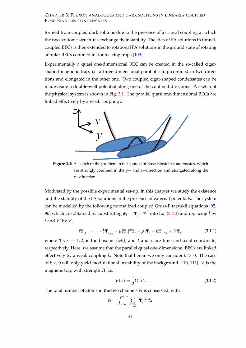
CHAPTER 3: FLUXON ANALOGUES AND DARK SOLITONS IN LINEARLY COUPLED
BOSE-EINSTEIN CONDENSATES
formed from coupled dark solitons due to the presence of a critical coupling at which
the two solitonic structures exchange their stability. The idea of FA solutions in tunnel-
coupled BECs is then extended to rotational FA solutions in the ground state of rotating
annular BECs confined in double-ring traps [109].
Experimentally a quasi one-dimensional BEC can be created in the so-called cigar-
shaped magnetic trap, i.e. a three-dimensional parabolic trap confined in two direc-
tions and elongated in the other one. Two coupled cigar-shaped condensates can be
made using a double-well potential along one of the confined directions. A sketch of
the physical system is shown in Fig. 3.1. The parallel quasi one-dimensional BECs are
linked effectively by a weak coupling k.
Figure 3.1: A sketch of the problem in the context of Bose-Einstein condensates, which
are strongly confined in the y− and z−direction and elongated along the
x−direction.
Motivated by the possible experimental set-up, in this chapter we study the existence
and the stability of the FA solutions in the presence of external potentials. The system
can be modelled by the following normalized coupled Gross-Pitaevskii equations [95,
96] which are obtained by substituting ψj = Ψje−iρ0 t into Eq. (2.7.3) and replacing t by
t and V ′ by V,
iΨjt = − 12 Ψjxx + µ|Ψj|2Ψj − ρ0Ψj − kΨ3−j + VΨj, (3.1.1)
where Ψj, j = 1, 2, is the bosonic field, and t and x are time and axial coordinate,
respectively. Here, we assume that the parallel quasi one-dimensional BECs are linked
effectively by a weak coupling k. Note that herein we only consider k > 0. The case
of k < 0 will only yield modulational instability of the background [110, 111]. V is the
magnetic trap with strength Ω, i.e.
V(x) =12
Ω2x2. (3.1.2)
The total number of atoms in the two channels N is conserved, with
N =∫ +∞
−∞∑
j=1,2|Ψj|2 dx.
41

CHAPTER 3: FLUXON ANALOGUES AND DARK SOLITONS IN LINEARLY COUPLED
BOSE-EINSTEIN CONDENSATES
Different works have been done in similar settings as (3.1.1). Spontaneous symme-
try breaking was analyzed in [112] when BECs are loaded in two parallel quasi-one-
dimensional traps fitted with optical lattices. Before the experimental birth of BEC,
the similar settings have been used in the study of stable defects in nonlinear patterns
known as optical domain walls [113]. The investigation of the separation of two far sep-
arated domain walls along with their stability limits were considered in [114]. Recently,
the studies were extended for the case when two components of BECs are coupled by
both linear and nonlinear terms [115].
Extending the work [95, 96], which was without the magnetic trap, i.e. Ω ≡ 0, in this
chapter, we are particularly interested in the effects of Ω > 0 to the localized excita-
tions.
When the two condensates are uncoupled, i.e. k = 0, the dynamics of a dark soliton
in BECs with magnetic trap has been considered before theoretically [116, 117] (see
also [118] and references therein) and experimentally [34, 97, 119–121]. Interesting phe-
nomena on the collective behavior of a quantum degenerate bosonic gas, such as soli-
ton oscillations [97, 119, 120] and frequency shifts due to soliton collisions [121] were
observed. A theoretical analysis based on variational formulation was developed in
[35, 72] that is in good agreement with numerics as well as with experiments (see, e.g.,
[122, 123]). A similar variational method will be derived here to explain the dynamics
of FA solutions.
3.2 Overview of the chapter
The present chapter is organized as follows. In the next section, we will give mathe-
matical expressions for the FA and the coupled dark soliton solutions. In Section 3.4,
we will solve the governing equations numerically and discuss the existence and sta-
bility of coupled dark soliton and FA solutions in the absence and presence of magnetic
trap. In Section 3.5, we will find an analytical formula for the dependence of the critical
coupling kce upon the velocity of the FA solution. Here, we will also solve the gov-
erning equations in moving coordinate frame and find numerically the values of kce
corresponding to different values of velocity v of FA solution and hence will present a
comparison between the numerical and the analytical results. In Section 3.6, we will de-
rive a variational formulation for the FA solutions so that their dynamical behaviours
can be studied analytically. Comparing the numerical and the analytical results, we
show good agreement between them. We then briefly summarize the results of the
chapter in the last section.
42

CHAPTER 3: FLUXON ANALOGUES AND DARK SOLITONS IN LINEARLY COUPLED
BOSE-EINSTEIN CONDENSATES
3.3 Fluxon analogues solution
A special solution in the study of long Josephson junction is the so-called Josephson
vortex. The analogue of Josephson vortex in Eq. (3.1.1) when V = 0 is given by [95]
Ψ1 = A tanh(Bx) + iCsech(Bx) = Ψ∗2 , (3.3.1)
where the parameters A, B and C are given as A = ±√
ρ0+kµ , B = 2
√k and C =
±√
ρ0−3kµ . In contrast to this solution, there exists a coupled dark soliton solution for
which the value of parameter A is same as above while B = ±√
ρ0 + k.
Josephson vortices (JV) are vortices of supercurrent. Conventionally, JV are the soliton
solutions of the non-linear sine-Gordon equation [124]. The investigation of non-linear
wave theory can be done efficiently with the superconducting Josephson junction [107].
The Josephson vortex, also called fluxon, is of great significance in long Josephson junc-
tions and has solitonic behavior. This robust and stable object can be controlled at high
speed and used as a basic bit in information processing systems [95].
The soliton (3.3.1) can be regarded as an analogue of Josephson fluxons [95, 96] as the
phase difference ϕ between the phases of Ψ1 and Ψ2 forms a spatial kink connecting
ϕ = 0 and ϕ = ±2π as shown in Fig. 3.2. In the following, solution (3.3.1) (and its
continuations) will be referred to as FA solutions. From the expression, it is clear that
an FA exists only for 0 < k < ρ0/3. For k > ρ0/3, the solution in (3.3.1) transforms
into dark soliton [95, 96] which exists for k > −ρ0. Thus the FA and the dark soliton
solutions coincide at k = ρ0/3 and hence k = ρ0/3 is the bifurcation point along the
family of dark solitons. In the following, we denote this critical coupling as kce.
3.4 Numerical computations
In this section we will find the static coupled dark soliton and the FA solutions in the
absence and presence of a magnetic trap and investigate their stability numerically.
3.4.1 Coupled one-dimensional GP equations with k > 0 and V = 0
We begin by considering the coupled system of GP equations with V = 0. In such a
case our Eq. (3.1.1) reduces to
iΨ1t +12 Ψ1xx − µ|Ψ1|2Ψ1 + ρ0Ψ1 + kΨ2 = 0,
iΨ2t +12 Ψ2xx − µ|Ψ2|2Ψ2 + ρ0Ψ2 + kΨ1 = 0.
(3.4.1)
43

CHAPTER 3: FLUXON ANALOGUES AND DARK SOLITONS IN LINEARLY COUPLED
BOSE-EINSTEIN CONDENSATES
−30 −20 −10 0 10 20 300
1
2
3
4
5
6
7
x
Ang
le(Ψ
1)−A
ngle
(Ψ2)
Figure 3.2: Spatial profile of the phase difference between Ψ1 and Ψ2 of FA solution
for k = 0.1 forming a 2π-kink shape.
For the steady state solution, putting Ψ1t = 0 = Ψ2t and then discretizing Ψ1xx and Ψ2xx
in Eq. (3.4.1), we obtain a coupled system of nonlinear algebraic equations which can
be solved using Newton’s method with the Neumann boundary conditions Ψj,0 = Ψj,1,
Ψj,N+1 = Ψj,N , j = 1, 2 to obtain numerically linearly coupled dark soliton solution
shown in Fig. 3.3.
3.4.2 Stability of dark soliton in coupled one-dimensional GP equations
Assume first that Ψ(0)1 and Ψ(0)
2 are the static solutions of Eq. (3.4.1). Then considering
small perturbations of these solutions in the form
Ψ1 = Ψ(0)1 (x) + ϵ[a1(x) eiλt + b∗1(x) e−iλ∗t], (3.4.2)
Ψ2 = Ψ(0)2 (x) + ϵ[a2(x) eiλt + b∗2(x) e−iλ∗t], (3.4.3)
and substituting these values of Ψ1 and Ψ2 into Eq. (3.4.1), we obtain the following
linearized equations
12
a1xx + ρ0a1 − 2µ|Ψ(0)1 |2a1 + ka2 − µ
(Ψ(0)
1
)2b1 = λa1, (3.4.4)
12
a2xx + ρ0a2 − 2µ|Ψ(0)2 |2a2 + ka1 − µ
(Ψ(0)
2
)2b2 = λa2, (3.4.5)
−12
b1xx − ρ0b1 + 2µ|Ψ(0)1 |2b1 − kb2 + µ
(Ψ(0)∗
1
)2a1 = λb1, (3.4.6)
−12
b2xx − ρ0b2 + 2µ|Ψ(0)2 |2b2 − kb1 + µ
(Ψ(0)∗
2
)2a2 = λb2. (3.4.7)
44

CHAPTER 3: FLUXON ANALOGUES AND DARK SOLITONS IN LINEARLY COUPLED
BOSE-EINSTEIN CONDENSATES
−30 −20 −10 0 10 20 30−2
0
2
xΨ
1
−30 −20 −10 0 10 20 30−2
0
2
x
Ψ2
Figure 3.3: Numerical solution of two coupled one-dimensional GP equations for µ =
1, ρ0 = 1, k = 0.3, ∆x = 0.2. The blue curves represent the real parts and
the black horizontal lines represent the imaginary parts of the solution.
The above system of Eq. (3.4.4), Eq. (3.4.5), Eq. (3.4.6) and Eq. (3.4.7) describes a linear
eigenvalue problem. Discretizing this system of equations and using the Neumann
boundary conditions aj,0 = aj,1, aj,N+1 = aj,N , bj,0 = bj,1, bj,N+1 = bj,N , where j=1,2, the
system can be written in matrix form.
We find the eigenvalues of the stability matrix in the complex plane for the solution
depicted in Fig. 3.3 and is shown in Fig. 3.4. Here, we have set ρ0 = 1. Because there
is at least one pair of eigenvalues with nonzero imaginary parts, we conclude that the
solitons are unstable. We have calculated the stability of dark solitons for different val-
ues of coupling constant k. The magnitude of the most unstable eigenvalues increases
with k up to k = 0.2 and then decreases and ultimately becomes zero for k ≥ 1/3. This
shows that the coupled dark solitons solution is stable for k ≥ 1/3 as shown in Fig. 3.5.
We also investigate the stability of coupled dark soliton in its domain of existence for
negative values of k. The dark soliton is found to be unstable for all negative values of
k.
To verify the above results, we solve Eq. (3.4.1) using Runge-Kutta method of order 4.
The time evolution of the coupled dark soliton in Fig. 3.3 for k = 0.1 is shown in Fig.
3.6. One can see that when t ≈ 40, energy releases in the form of radiation due to the
instability of solitons. Here, the energy splits into three parts. Some part of energy goes
to the right, some towards left and the remaining goes straight. The time dynamics of
the solution for different values of time is shown in Fig. 3.7.
45

CHAPTER 3: FLUXON ANALOGUES AND DARK SOLITONS IN LINEARLY COUPLED
BOSE-EINSTEIN CONDENSATES
−40 −20 0 20 40−0.2
−0.15
−0.1
−0.05
0
0.05
0.1
0.15
0.2
Re(λ)
Im(λ
)
Figure 3.4: The eigenvalues λ of the solution in Fig. 3.3 in the complex plane showing
the instability of the solution.
0 0.2 0.4 0.6 0.8 10
0.05
0.1
0.15
0.2
0.25
0.3
0.35
k
Max
(Im
(λ))
Figure 3.5: The critical eigenvalue of coupled dark solitons shown in Fig. 3.3 as a func-
tion of k.
46

CHAPTER 3: FLUXON ANALOGUES AND DARK SOLITONS IN LINEARLY COUPLED
BOSE-EINSTEIN CONDENSATES
x
t
−20 0 20
10
20
30
40
50
60
xt
−20 0 20
10
20
30
40
50
60
0.2
0.4
0.6
0.8
1
0.2
0.4
0.6
0.8
1
Figure 3.6: An evolution of the unstable coupled dark solitons shown in Fig. 3.3. The
left panel corresponds to |Ψ1| and right panel to |Ψ2|.
−200
20
0
50
100
1500
0.5
1
1.5
xt
|Ψ1|
−200
20
0
50
100
1500
0.5
1
1.5
xt
|Ψ2|
Figure 3.7: Time evolution of the unstable coupled dark solitons shown in Fig. 3.3 for
few particular values of time.
47

CHAPTER 3: FLUXON ANALOGUES AND DARK SOLITONS IN LINEARLY COUPLED
BOSE-EINSTEIN CONDENSATES
−30 −20 −10 0 10 20 30−2
0
2
xΨ
1
−30 −20 −10 0 10 20 30−2
0
2
x
Ψ2
Figure 3.8: A numerically obtained FA for ρ0 = 1, µ = 1, and k = 0.1. The blue curves
represent the real parts while the black curves are the imaginary parts of
Ψ1 and Ψ2, respectively.
3.4.3 Existence of fluxon analogues solution
According to Kaurov and Kuklov [95], in the instability region of coupled dark soliton
one can obtain an FA. The numerically obtained FA solution is shown in Fig. 3.8 which
is the same solution given in Eq. (3.3.1). We observe that the amplitude of the real parts
of the FA solution increases with k. However, the amplitude of the imaginary parts of
FA solution decreases with k. As k approaches 1/3, the amplitude of the humps in the
imaginary parts tends to zero and the FA solution changes into a coupled dark solitons
solution. This shows that the FA solution exists for k < 1/3 and at k = kce = 1/3, it
transforms into a coupled dark solitons solution, where kce represents the critical value
of existence of the solution. The transformation of FA into a coupled dark solitons can
be comprehended as a pitchfork bifurcation as shown in Fig. 3.9.
3.4.4 Stability of fluxon analogues solution
Following the same procedure as the stability of coupled dark solitons, we investigate
the stability of FA solution. The eigenvalues of the stability matrix for the FA solution
are shown in Fig. 3.10. This shows that the FA solution is stable for k = 0.1. We observe
that the FA solution indeed remains stable for those values of k where it exists. We
also note that in Fig. 3.6, a grey-soliton-like structure in the centre at the end of the
computation is an FA, as the profile of the phase difference between Ψ1 and Ψ2 forms
48

CHAPTER 3: FLUXON ANALOGUES AND DARK SOLITONS IN LINEARLY COUPLED
BOSE-EINSTEIN CONDENSATES
0.2 0.4 0.6 0.8 1−1
−0.5
0
0.5
1
k
Max
/Min
(Im
(Ψj))
Figure 3.9: The hump amplitude of the imaginary parts of FA solution shown in Fig.
3.8 against k. The graph depicts the region of existence of FA solution.
The blue and black curves correspond to the imaginary parts of Ψ1 and Ψ2
while the red line in the middle is for the coupled dark solitons.
a 2π-kink shape as depicted in Fig. 3.2. Nonetheless, it is important to note that it is
not always the case. When the coupling constant is too small, instead of yielding FA
solutions, the dark solitons repel and move away from each other as shown in Fig.
3.11. Hence, coupled dark solitons transform into FA solutions if the coupling is in an
intermediate region.
3.4.5 Coupled BECs with a trap: V = 0
Next, we consider the existence and stability of FA solution in the presence of a har-
monic trap, i.e. Ω = 0. Two FA solutions for two different values of coupling constant
k are shown in Fig. 3.12 and Fig. 3.13 with Ω = 0.1. The value of Ω corresponds to the
width of the trap. First we take Ω = 0.05 which means that the width of the trap is
large. Then we decrease the width of the trap by increasing the value of Ω. We con-
sider Ω = 0.1, 0.15 and 0.2 and find the FA solution for each mentioned value of Ω. It
is found that the critical values kce where FA solution transforms into a dark soliton for
Ω = 0.05, 0.1, 0.15, 0.2 are 0.333, 0.334, 0.336, 0.337 respectively. These values show that
the critical coupling kce above which FA solutions do not exist is almost independent of
the trapping parameter Ω, which is reasonable as the width of the non-zero imaginary
part of the FA solution is small compared to the width of the trapping parameter Ω
when k → kce. The coupled dark soliton for a specific value of Ω is shown in Fig. 3.14.
49
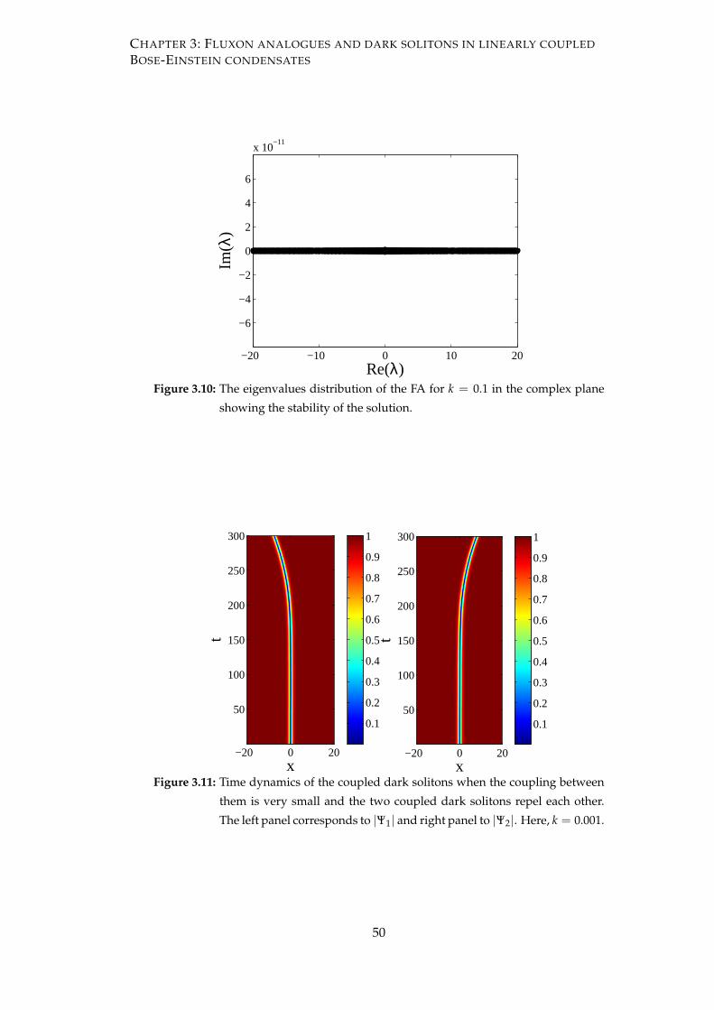
CHAPTER 3: FLUXON ANALOGUES AND DARK SOLITONS IN LINEARLY COUPLED
BOSE-EINSTEIN CONDENSATES
−20 −10 0 10 20
−6
−4
−2
0
2
4
6
x 10−11
Re(λ)
Im(λ
)
Figure 3.10: The eigenvalues distribution of the FA for k = 0.1 in the complex plane
showing the stability of the solution.
x
t
−20 0 20
50
100
150
200
250
300
x
t
−20 0 20
50
100
150
200
250
300
0.1
0.2
0.3
0.4
0.5
0.6
0.7
0.8
0.9
1
0.1
0.2
0.3
0.4
0.5
0.6
0.7
0.8
0.9
1
Figure 3.11: Time dynamics of the coupled dark solitons when the coupling between
them is very small and the two coupled dark solitons repel each other.
The left panel corresponds to |Ψ1| and right panel to |Ψ2|. Here, k = 0.001.
50

CHAPTER 3: FLUXON ANALOGUES AND DARK SOLITONS IN LINEARLY COUPLED
BOSE-EINSTEIN CONDENSATES
−40 −20 0 20 40−1
0
1
xΨ
1
−40 −20 0 20 40−1
0
1
x
Ψ2
Figure 3.12: A numerically obtained FA solution for Ω = 0.1, ρ0 = 1, µ = 1 and
k = 0.1. The blue solid curves represent the real parts and the black solid
curves are the imaginary parts of the FA solution. The dash-dotted curves
are approximations (see Section 3.6, Eq. (3.6.1)).
−40 −20 0 20 40−1
0
1
x
Ψ1
−40 −20 0 20 40−1
0
1
x
Ψ2
Figure 3.13: A numerically obtained FA solution for the same parameter values as in
Fig. 3.12 but k = 0.008. The blue solid curves represent the real parts
and the black solid curves are the imaginary parts of the FA solution.
The dash-dotted curves and the dashed curves are two approximations
obtained through different approaches (see Section 3.6, Eqs. (3.6.1) and
(3.6.19) respectively).
51
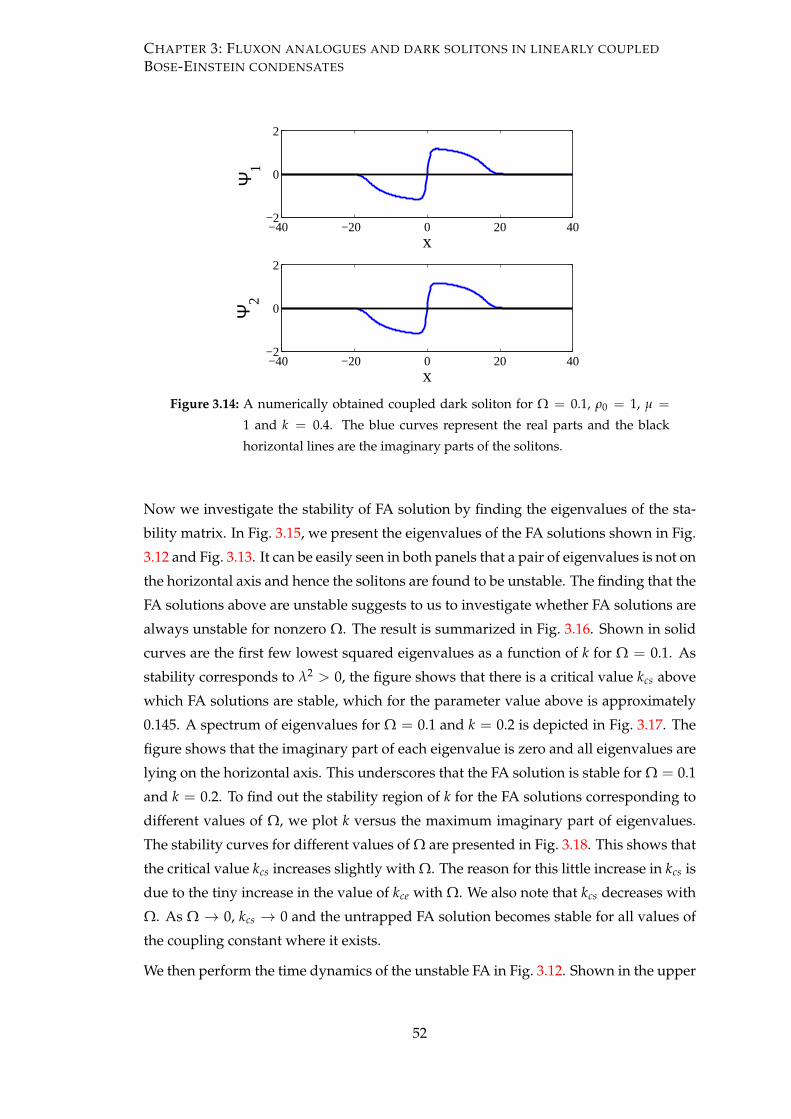
CHAPTER 3: FLUXON ANALOGUES AND DARK SOLITONS IN LINEARLY COUPLED
BOSE-EINSTEIN CONDENSATES
−40 −20 0 20 40−2
0
2
xΨ
1
−40 −20 0 20 40−2
0
2
x
Ψ2
Figure 3.14: A numerically obtained coupled dark soliton for Ω = 0.1, ρ0 = 1, µ =
1 and k = 0.4. The blue curves represent the real parts and the black
horizontal lines are the imaginary parts of the solitons.
Now we investigate the stability of FA solution by finding the eigenvalues of the sta-
bility matrix. In Fig. 3.15, we present the eigenvalues of the FA solutions shown in Fig.
3.12 and Fig. 3.13. It can be easily seen in both panels that a pair of eigenvalues is not on
the horizontal axis and hence the solitons are found to be unstable. The finding that the
FA solutions above are unstable suggests to us to investigate whether FA solutions are
always unstable for nonzero Ω. The result is summarized in Fig. 3.16. Shown in solid
curves are the first few lowest squared eigenvalues as a function of k for Ω = 0.1. As
stability corresponds to λ2 > 0, the figure shows that there is a critical value kcs above
which FA solutions are stable, which for the parameter value above is approximately
0.145. A spectrum of eigenvalues for Ω = 0.1 and k = 0.2 is depicted in Fig. 3.17. The
figure shows that the imaginary part of each eigenvalue is zero and all eigenvalues are
lying on the horizontal axis. This underscores that the FA solution is stable for Ω = 0.1
and k = 0.2. To find out the stability region of k for the FA solutions corresponding to
different values of Ω, we plot k versus the maximum imaginary part of eigenvalues.
The stability curves for different values of Ω are presented in Fig. 3.18. This shows that
the critical value kcs increases slightly with Ω. The reason for this little increase in kcs is
due to the tiny increase in the value of kce with Ω. We also note that kcs decreases with
Ω. As Ω → 0, kcs → 0 and the untrapped FA solution becomes stable for all values of
the coupling constant where it exists.
We then perform the time dynamics of the unstable FA in Fig. 3.12. Shown in the upper
52

CHAPTER 3: FLUXON ANALOGUES AND DARK SOLITONS IN LINEARLY COUPLED
BOSE-EINSTEIN CONDENSATES
−20 −10 0 10 20−0.05
0
0.05
Re(λ)
Im(λ
)
(a)
−20 −10 0 10 20−0.2
−0.15
−0.1
−0.05
0
0.05
0.1
0.15
Re(λ)
Im(λ
)
(b)
Figure 3.15: Eigenvalues structures for the FA solutions shown in Fig. 3.12 and Fig.
3.13 respectively. A pair of eigenvalues in both panels is lying on the
vertical axis showing the instability of the solutions.
53

CHAPTER 3: FLUXON ANALOGUES AND DARK SOLITONS IN LINEARLY COUPLED
BOSE-EINSTEIN CONDENSATES
0.1 0.2 0.3 0.4 0.5−0.1
−0.08
−0.06
−0.04
−0.02
0
0.02
k
λ2
Figure 3.16: The first few lowest squared eigenvalues of FA (solid) and dark solitons
(dashed) as a function of k for Ω = 0.1. The dash-dotted curve represents
the approximation (3.6.17).
−40 −20 0 20 40
−6
−4
−2
0
2
4
6
x 10−8
Re(λ)
Im(λ
)
Figure 3.17: Eigenvalues structure showing the stability of the FA solution for Ω = 0.1
and k = 0.2.
54

CHAPTER 3: FLUXON ANALOGUES AND DARK SOLITONS IN LINEARLY COUPLED
BOSE-EINSTEIN CONDENSATES
0.1 0.12 0.14 0.16 0.18 0.20
0.02
0.04
0.06
0.08
0.1
0.12
k
Max
(Im
(λ))
Ω=0.05Ω=0.1Ω=0.15Ω=0.2
Figure 3.18: Stability curves for FA solutions corresponding to Ω = 0.05, 0.1, 0.15, 0.2.
For each value of Ω, there is a little change in the value of kcs.
panel of Fig. 3.19 is the typical evolution of unstable FA, where one can see that the in-
stability causes the solitons to oscillate about the minimum of the trap non-sinusoidally.
Hence, despite the instability, the FA still persists. This result rather applies generally
to other values of coupling constants where FA solutions are unstable. The numerical
evolution of the phase difference for k = 0.1 is shown in the lower panel of Fig. 3.19.
Clearly the phase difference varies from −2π to 0 which indicates the existence of FA.
We have also studied the existence and the stability of dark solitons. Shown as dashed
lines in Fig. 3.16 are the first few lowest squared eigenvalues of coupled dark solitons,
where similarly as before for k less than the critical coupling kce coupled dark solitons
may transform into an FA as shown in Fig. 3.20.
3.5 Travelling FA solutions and the velocity dependence of the
critical coupling kce
Because solitons of Eq. (3.1.1) without a trap are translationally invariant, they can
move freely in space. This motivates us to study the existence and stability of moving
solitons.
When FA solutions do not travel, it has been discussed above that kce = 1/3. When
the solitons move with velocity v, it is natural to expect that the domain of existence of
FA solutions will depend on v, i.e. kce = kce(v). It is because dark solitons only exist
for v < 1 [72], while at kce FA solutions become dark solitons. In the following, we
55

CHAPTER 3: FLUXON ANALOGUES AND DARK SOLITONS IN LINEARLY COUPLED
BOSE-EINSTEIN CONDENSATES
t
x−20 0 20
100
200
300
400
500
600
t
x−20 0 20
100
200
300
400
500
600
0.2
0.4
0.6
0.8
1
0.2
0.4
0.6
0.8
1
(a)
x
t
−10 −5 0 5 10
50
100
150
200
250
300
−6
−5
−4
−3
−2
−1
0
(b)
Figure 3.19: The upper panel shows a numerical evolution of the FA in Fig. 3.12 for
Ω = 0.1 and k = 0.1. The lower panel shows a numerical evolution of the
phase difference for the same parameter values above. The phase changes
from −2π to 0 and shows the presence of FA solution.
56

CHAPTER 3: FLUXON ANALOGUES AND DARK SOLITONS IN LINEARLY COUPLED
BOSE-EINSTEIN CONDENSATES
x
t
−20 0 20
50
100
150
200
x
t
−20 0 20
50
100
150
200
0.2
0.4
0.6
0.8
1
0.2
0.4
0.6
0.8
1
Figure 3.20: A numerical evolution of coupled dark solitons for Ω = 0.1 and k = 0.1.
are interested in the expression of the critical coupling. We will determine the velocity
dependence of kce analytically.
For simplicity, first we scale the governing Eq. (3.1.1) such that the nonlinearity coeffi-
cient and the chemical potential become µ = ρ0 = 1. We also scale the wavefunction
Ψj, where j=1,2, by ψj = Ψj/√
1 + k, such that the Eq. (3.1.1) become
iψ1t +12
ψ1xx − |ψ1|2ψ1 +ψ1 + kψ2
1 + k=
Vψ1
1 + k, (3.5.1)
iψ2t +12
ψ2xx − |ψ2|2ψ2 +ψ2 + kψ1
1 + k=
Vψ2
1 + k. (3.5.2)
where t = (1 + k)t and x = (√
1 + kx).
Defining ξ = x − vt, Eq. (3.5.1) and Eq. (3.5.2) with V = 0 in a moving coordinate frame
can be written as
iψ1t − ivψ1ξ +12
ψ1ξξ − |ψ1|2ψ1 +ψ1 + kψ2
1 + k= 0, (3.5.3)
iψ2t − ivψ2ξ +12
ψ2ξξ − |ψ2|2ψ2 +ψ2 + kψ1
1 + k= 0. (3.5.4)
When ψ1 = ψ2 = ψ, the above system of equations has an explicit solution for the
travelling dark soliton
ψds = A tanh(Bξ) + iv, (3.5.5)
with A = B and A2 + v2 = 1.
Let us perturb ψds such that ψ1 = ψds + ϵ f (ξ) and ψ2 = ψds − ϵ f (ξ), where ϵ ≪ 1.
Substituting these values of ψ1 and ψ2 into Eq. (3.5.3) and Eq. (3.5.4) and retaining
57
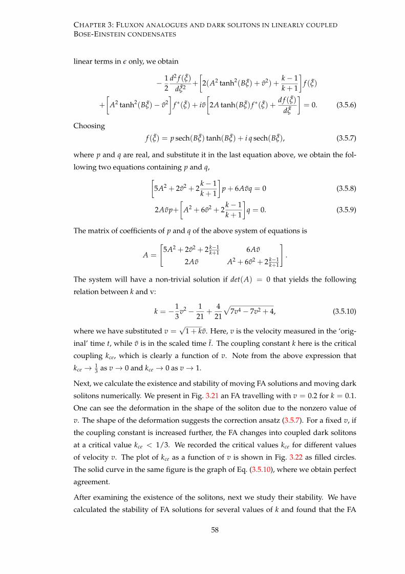
CHAPTER 3: FLUXON ANALOGUES AND DARK SOLITONS IN LINEARLY COUPLED
BOSE-EINSTEIN CONDENSATES
linear terms in ϵ only, we obtain
− 12
d2 f (ξ)dξ2
+
[2(A2 tanh2(Bξ) + v2) +
k − 1k + 1
]f (ξ)
+
[A2 tanh2(Bξ)− v2
]f ∗(ξ) + iv
[2A tanh(Bξ) f ∗(ξ) +
d f (ξ)dξ
]= 0. (3.5.6)
Choosing
f (ξ) = p sech(Bξ) tanh(Bξ) + i q sech(Bξ), (3.5.7)
where p and q are real, and substitute it in the last equation above, we obtain the fol-
lowing two equations containing p and q,[5A2 + 2v2 + 2
k − 1k + 1
]p + 6Avq = 0 (3.5.8)
2Avp+[
A2 + 6v2 + 2k − 1k + 1
]q = 0. (3.5.9)
The matrix of coefficients of p and q of the above system of equations is
A =
[5A2 + 2v2 + 2 k−1
k+1 6Av
2Av A2 + 6v2 + 2 k−1k+1
].
The system will have a non-trivial solution if det(A) = 0 that yields the following
relation between k and v:
k = −13
v2 − 121
+4
21
√7v4 − 7v2 + 4, (3.5.10)
where we have substituted v =√
1 + kv. Here, v is the velocity measured in the ‘orig-
inal’ time t, while v is in the scaled time t. The coupling constant k here is the critical
coupling kce, which is clearly a function of v. Note from the above expression that
kce → 13 as v → 0 and kce → 0 as v → 1.
Next, we calculate the existence and stability of moving FA solutions and moving dark
solitons numerically. We present in Fig. 3.21 an FA travelling with v = 0.2 for k = 0.1.
One can see the deformation in the shape of the soliton due to the nonzero value of
v. The shape of the deformation suggests the correction ansatz (3.5.7). For a fixed v, if
the coupling constant is increased further, the FA changes into coupled dark solitons
at a critical value kce < 1/3. We recorded the critical values kce for different values
of velocity v. The plot of kce as a function of v is shown in Fig. 3.22 as filled circles.
The solid curve in the same figure is the graph of Eq. (3.5.10), where we obtain perfect
agreement.
After examining the existence of the solitons, next we study their stability. We have
calculated the stability of FA solutions for several values of k and found that the FA
58

CHAPTER 3: FLUXON ANALOGUES AND DARK SOLITONS IN LINEARLY COUPLED
BOSE-EINSTEIN CONDENSATES
−20 −10 0 10 20−1
0
1
x
ψ1
−20 −10 0 10 20−1
0
1
x
ψ2
Figure 3.21: A numerically obtained FA for v = 0.2 and k = 0.1.
0 0.05 0.1 0.15 0.2 0.25 0.3 0.350
0.2
0.4
0.6
0.8
1
kce
v
Figure 3.22: The critical coupling constant kce as a function of the velocity v for the
existence of travelling FA. Filled circles are numerical data and the solid
line is the function in Eq. (3.5.10). FA only exists on the left of the solid
curve.
59

CHAPTER 3: FLUXON ANALOGUES AND DARK SOLITONS IN LINEARLY COUPLED
BOSE-EINSTEIN CONDENSATES
solutions are always stable in their existence domain. Extending the calculation to
coupled dark solitons, we found that they are unstable for the values of the coupling
constant k < kce corresponding to each value of the velocity v. For the values of k ≥ kce,
the dark soliton becomes stable. The Runge-Kutta method of order 4 has been used to
verify the time dynamics of the FA solutions as well as dark solitons. The typical time
evolution of the coupled dark soliton solution when it is unstable is depicted in the
upper panel of Fig. 3.23. The lower panel of Fig. 3.23 shows the time evolution of the
stable FA solution.
3.6 Variational formulations of the FA solutions
Here, we will derive theoretical approximations to the numerical existence and stability
results reported above using variational methods. The Lagrangian formalism for the
FA solutions will be separated into two cases, i.e. when the coupling constant k is close
to the critical coupling kce at which the FA solutions are close to coupled dark solitons
and when it is close to the uncoupled limit k ≈ 0. The two cases determine the ansatz
that will be taken to approximate the solutions.
3.6.1 The case k ∼ kce and V = 0
When there is a harmonic potential, the dynamics of the solutions will be determined
perturbatively. We will particularly follow the method of [72, 122, 123], which was
developed for dark solitons, to our case. A similar calculation will be performed to
discuss the dynamics and stability of FA solutions in the limit of k close to kce as in that
case the real part, i.e. the dark soliton component, is dominant and C1, C2 ≈ 0.
Due to the presence of the magnetic trap, which is assumed to be slowly varying, i.e.
Ω2 ≪ 1, we take the ansatz
Ψj = ΨTFΦj, (3.6.1)
where ΨTF is the Thomas-Fermi cloud approximately given by
ΨTF =√
max(1 − V/(1 + k)), 0. (3.6.2)
and
Φj = A tanh (z) + i(Cjsech (z) + v
), j = 1, 2, (3.6.3)
where z = B (x − x0). The parameters A, B, C, x0 are in general functions of t. Here,
A2 + v2 = 1. When Cj ≡ 0, one can recognise that the above function is the usual
60

CHAPTER 3: FLUXON ANALOGUES AND DARK SOLITONS IN LINEARLY COUPLED
BOSE-EINSTEIN CONDENSATES
ξ
t
−20 0 20
20
40
60
80
100
120
140
160
180
200
ξ
t
−20 0 20
20
40
60
80
100
120
140
160
180
200
0.2
0.4
0.6
0.8
1
0.3
0.4
0.5
0.6
0.7
0.8
0.9
1
1.1
(a)
ξ
t
−20 0 20
20
40
60
80
100
120
140
160
180
200
ξ
t
−20 0 20
20
40
60
80
100
120
140
160
180
200
0.2
0.3
0.4
0.5
0.6
0.7
0.8
0.9
1
0.88
0.9
0.92
0.94
0.96
0.98
1
1.02
1.04
(b)
Figure 3.23: Time dynamics of the travelling coupled dark solitons and the travelling
FA for the parameter values k = 0.1 and v = 0.2. The upper panel shows
the instability of the coupled dark solitons and the lower panel depicts
the stability of travelling FA solution.
61

CHAPTER 3: FLUXON ANALOGUES AND DARK SOLITONS IN LINEARLY COUPLED
BOSE-EINSTEIN CONDENSATES
ansatz to describe a dark soliton travelling with the velocity v, where in that case the
parameters A, B, v and x0 can be conveniently written as A = B = cos φ, v = sin φ,
and x0(t) =∫ t
0 sin φ(t′) dt′ [122].
Note the similarity of Eq. (3.6.1) with the ansatz Ψj = ΨTFψds [122, 123] used to study
the dynamics of dark solitons in a harmonic potential. Differentiating the ansatz (3.6.1)
with respect to t and x, we obtain
Ψjt = ΨTFΦjt,
Ψjxx =−ΦjVx
2
4 (1 + k)2 (1 − V1+k
)3/2 −ΦjxVx
(1 + k)√
1 − V1+k
−ΦjVxx
2 (1 + k)√
1 − V1+k
+
√1 − V
1 + kΦjxx.
Substituting the ansatz (3.6.1) and its spatial and temporal derivatives into Eq. (3.5.1)
and Eq. (3.5.2), we obtain
i√
1 − V1 + k
Φjt +12
[ −ΦjVx2
4 (1 + k)2 (1 − V1+k
)3/2 −ΦjxVx
(1 + k)√
1 − V1+k
−ΦjVxx
2 (1 + k)√
1 − V1+k
+
√1 − V
1 + kΦjxx
]−(
1 − V1 + k
)3/2
|Φj|2Φj
+
√1 − V
1+k
(Φj + kΦ3−j
)1 + k
=VΦj
√1 − V
1+k
1 + k.
Dividing both sides by√
1 − V1+k , we obtain
iΦjt −ΦjVx
2
8 (1 + k)2 (1 − V1+k
)2 −ΦjxVx
2 (1 + k)(1 − V
1+k
) − ΦjVxx
4 (1 + k)(1 − V
1+k
)+
12
Φjxx −(
1 − V1 + k
)|Φj|2Φj +
(Φj + kΦ3−j
)1 + k
=VΦj
1 + k.
Using the Taylor series expansion of 11− V
1+kand retaining only terms linear in V, Vx and
Vxx due to smallness of trapping parameter, we obtain
iΦj t +12
Φj xx − |Φj|2Φj +Φj + kΦ3−j
1 + k≈ R(Φj), (3.6.4)
where
R(Φj) =1
(1 + k)
[(1 − |Φj|2
)VΦj +
12
VxΦj x +14
ΦjVxx
].
When there is no magnetic trap, (3.6.4) with V ≡ 0 can be derived from the Lagrangian
L =∫ ∞
−∞
12
2
∑j=1
i(
Φ∗j Φj t − ΦjΦ∗
j t
)(1 − 1
|Φj|2
)− |Φj x|
2 −(|Φj|4 − 1
)+2
|Φj|2 + kΦjΦ∗3−j − (1 + k)
1 + kdx. (3.6.5)
62

CHAPTER 3: FLUXON ANALOGUES AND DARK SOLITONS IN LINEARLY COUPLED
BOSE-EINSTEIN CONDENSATES
It is not clear how to evaluate the first term of the integral (3.6.5) due to the presence
of nonzero Cj in the denominator of(1 − 1/|Φj|2
). Because of that, in the following
we assume Cj to be small, i.e. we consider the case of k ∼ kce, and take the series
expansion with respect to Cj about Cj = 0 upto O(C5j ). The integral of the first term of
the Lagrangian density is
∫ ∞
−∞
12
2
∑j=1
i(
Φ∗j Φj t − ΦjΦ∗
j t
)(1 − 1
|Φj|2
)dx = x0t
[4 arctan
(Av
)− 4Av − πAC3
].
(3.6.6)
The integral of the second term yields
∫ ∞
−∞
12
2
∑j=1
|Φj x|2 dx =
B3
[4A2 + C4
]. (3.6.7)
The integral of the third term leads to
∫ ∞
−∞
12
2
∑j=1
(|Φj|4 − 1
)dx =
13B
[4A4 − 12A2 + 3πvC3(2 − A2) + 2C4(9 − 8A2)
+ 3πvC5 + 2C6
]. (3.6.8)
The integral of the last term yields
∫ ∞
−∞
2
∑j=1
|Φj|2 + kΦjΦ∗3−j − (1 + k)
1 + kdx = − 2
B(1 + k)
[2A2(2k + 1)− 2kC1C2
− πvC3(1 + k)]
. (3.6.9)
After, performing all the integrations, the following effective Lagrangian is obtained
Le f f = x0 t
[− 4Av + 4 tan−1
(Av
)− πAC3
]− 4
3BA2 (A2 + B2)
+πvB
(A2C3 − C5)−1
3B
[ (B2 − 16A2)C4 + 2C6
]− 2
B(1 + k)
[(3k + 2)C4 − 2kC1C2
]+O(C5
j ), (3.6.10)
where C2+r = (C1)r + (C2)r, r = 1, . . . , 4. One can check that when the soliton is not
moving, i.e. x0 t = v = 0 and A = 1, the Euler-Lagrange equations for the remaining
parameters B, C1, and C2 are
2Cj
(B2 + 4Cj
2)(1 + k) + 4Cj (k − 2)− 12kC3−j = 0, (3.6.11)
(1 + k)[
2(C6 + 2)− B2(C4 + 4)]− 4(C4 + 3kC1C2) + 2kC4 = 0. (3.6.12)
63

CHAPTER 3: FLUXON ANALOGUES AND DARK SOLITONS IN LINEARLY COUPLED
BOSE-EINSTEIN CONDENSATES
The equations can be solved analytically to yield
B(0) =2√
k√1 + k
, C(0)1 = −C(0)
2 = ±√
1 − 3k√1 + k
, (3.6.13)
which is nothing else, but the FA solution or B(0) = 1, C(0)j = 0, which is the dark
soliton. It is important to note here that despite the series expansion with respect to Cj
that we took prior to integrating Eq. (3.6.5), our result (3.6.13) corresponds to an exact
solution for any value of 0 < k ≤ kce. It is not yet clear to us why this is the case.
To determine the influence of the magnetic trap, i.e. V = 0, to the FA solutions, we
will follow [72], where the perturbation-induced dynamics of dark solitons using a
variational approach was discussed. The Euler-Lagrange equations of motion were
derived for a perturbed nonlinear Schrödinger equation similar to Eq. (3.6.4). In our
case, we treat the right hand side of Eq. (3.6.4) as perturbations. Due to the presence of
the perturbations the Euler-Lagrange equation for the variable αj, with αj = φ, B, and
Cj, becomes [72]
∂Le f f
∂αj− ∂t
∂Le f f
∂αj t= 2 Re
(∫ ∞
−∞
2
∑j=1
R(Φj)∗ ∂Φj
∂αjdx
).
Following [117, 122], we need two active variables only. Because of that, we will assume
that adiabatically B and Cj are independent of time and are given by Eq. (3.6.13). Hence,
we obtain the following set of equations
dAdt
=Ω2x0v
12√
k(k + 1)52
[A2(k + 1) + 11k − 1
], (3.6.14)
dx0
dt=
v
576Ak32 (k + 1)
52
[192k4(A2 + 14) + 576k3(A2 + 8) + 576k2(A2 + 2)
+ Ω2k2(48x0
2 + π2)(A2 + 3) + 12(A2 + 9)
+ 2kΩ2
24x02(A2 − 1) + 12(A2 + 4) + π2(A2 + 1)
+ Ω2(A2 − 1)(π2 + 12) + 192k(A2 − 4)
]. (3.6.15)
From the two equations above, we obtain
d2x0
dt2 =−x0Ω2
144(k + 1)5
[Ω2(π2 + 30)(k + 1) + 36(20k3 + 36k2 + 12k − 4)
+48Ω2x02k]
, (3.6.16)
Ignoring the terms containing Ω4 since Ω2 ≪ 1, we are left with
d2x0
dt2 =(1 − 5k)Ω2
1 + kx0, (3.6.17)
64

CHAPTER 3: FLUXON ANALOGUES AND DARK SOLITONS IN LINEARLY COUPLED
BOSE-EINSTEIN CONDENSATES
where we have assumed that A ≈ 1 and x0 ≈ 0. Note that the derivative in Eq.
(3.6.17) is with respect to the original time variable. This shows that the solution is
stable for values of k > 15 . When k = 1/3, we recover the oscillation frequency of dark
solitons in a harmonic trap [125] (see also [97, 117, 122]). We checked the validity of our
approximation by comparing it with numerical results in Fig. 3.16 where qualitatively
a good approximation is obtained.
3.6.2 The case k ∼ 0 and V = 0
When k is close to zero, the imaginary part of the FA solution is dominant over the
real part. Due to the presence of a magnetic trap, the imaginary part will become
the Thomas-Fermi ground state in the limit k → 0. Motivated by, e.g., [126] where a
Gaussian ansatz, which is the ground state solution of the linear Schrödinger equations
(3.1.1) and (3.1.2) with k = 0, was shown to be able to approximate the ground state of
the nonlinear equation, in the following we will take a similar ansatz for our problem.
For the present case, we will consider the governing equation (3.1.1) to be derived from
the Lagrangian
L =∫ ∞
−∞
12
2
∑j=1
i(
Ψ∗j Ψjt − ΨjΨ∗
j t
)− |Ψjx|
2 − µ|Ψj|4
+2 (ρ0 − V) |Ψj|2 + 2kΨjΨ∗3−j dx. (3.6.18)
Note that the main difference between Eq. (3.6.18) and Eq. (3.6.5) is the factor(
1 − 1|Ψj|2
)in the first term of the integrand. As for the ansatz, we take
Ψj =(
Ajx + iCj)
e−Bx2. (3.6.19)
The advantage of such a Gaussian ansatz is that the Lagrangian can be evaluated rather
straightforwardly.
We substitute the ansatz into the Lagrangian (3.6.18) and evaluate the integral term by
term. The integral of the first term is zero. The integral of the second term is∫ ∞
−∞
12
2
∑j=1
|Ψjx|2 =1
16
√2π
B[3A3 + 4BC4] . (3.6.20)
The integral of the third term yields∫ ∞
−∞
12
2
∑j=1
µ|Ψj|4 =µ√
π
256B5/2
[64B2C6 + 16BA6 + 3A4
]. (3.6.21)
The integral of the fourth term leads to∫ ∞
−∞
2
∑j=1
(ρ0 − V)|Ψj|2 =
√2π
32B5/2
[A3(8ρ0B − 3Ω2) + 4BC4(8ρ0B − Ω2)
]. (3.6.22)
65
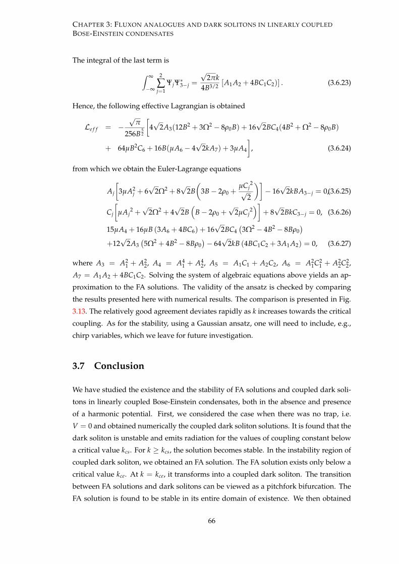
CHAPTER 3: FLUXON ANALOGUES AND DARK SOLITONS IN LINEARLY COUPLED
BOSE-EINSTEIN CONDENSATES
The integral of the last term is
∫ ∞
−∞
2
∑j=1
ΨjΨ∗3−j =
√2πk
4B3/2 [A1 A2 + 4BC1C2)] . (3.6.23)
Hence, the following effective Lagrangian is obtained
Le f f = −√
π
256B52
[4√
2A3(12B2 + 3Ω2 − 8ρ0B) + 16√
2BC4(4B2 + Ω2 − 8ρ0B)
+ 64µB2C6 + 16B(µA6 − 4√
2kA7) + 3µA4
], (3.6.24)
from which we obtain the Euler-Lagrange equations
Aj
[3µA2
j + 6√
2Ω2 + 8√
2B(
3B − 2ρ0 +µCj
2
√2
)]− 16
√2kBA3−j = 0,(3.6.25)
Cj
[µAj
2 +√
2Ω2 + 4√
2B(
B − 2ρ0 +√
2µCj2)]
+ 8√
2BkC3−j = 0, (3.6.26)
15µA4 + 16µB (3A6 + 4BC6) + 16√
2BC4(3Ω2 − 4B2 − 8Bρ0
)+12
√2A3
(5Ω2 + 4B2 − 8Bρ0
)− 64
√2kB (4BC1C2 + 3A1 A2) = 0, (3.6.27)
where A3 = A21 + A2
2, A4 = A41 + A4
2, A5 = A1C1 + A2C2, A6 = A21C2
1 + A22C2
2 ,
A7 = A1A2 + 4BC1C2. Solving the system of algebraic equations above yields an ap-
proximation to the FA solutions. The validity of the ansatz is checked by comparing
the results presented here with numerical results. The comparison is presented in Fig.
3.13. The relatively good agreement deviates rapidly as k increases towards the critical
coupling. As for the stability, using a Gaussian ansatz, one will need to include, e.g.,
chirp variables, which we leave for future investigation.
3.7 Conclusion
We have studied the existence and the stability of FA solutions and coupled dark soli-
tons in linearly coupled Bose-Einstein condensates, both in the absence and presence
of a harmonic potential. First, we considered the case when there was no trap, i.e.
V = 0 and obtained numerically the coupled dark soliton solutions. It is found that the
dark soliton is unstable and emits radiation for the values of coupling constant below
a critical value kcs. For k ≥ kcs, the solution becomes stable. In the instability region of
coupled dark soliton, we obtained an FA solution. The FA solution exists only below a
critical value kce. At k = kce, it transforms into a coupled dark soliton. The transition
between FA solutions and dark solitons can be viewed as a pitchfork bifurcation. The
FA solution is found to be stable in its entire domain of existence. We then obtained
66
CHAPTER 3: FLUXON ANALOGUES AND DARK SOLITONS IN LINEARLY COUPLED
BOSE-EINSTEIN CONDENSATES
a travelling FA and determined the range of values of the coupling constant k where
they exist. An explicit relation between the velocity v of the FA and its corresponding
critical value of existence kce is obtained analytically. The relation is compared with the
numerical results showing excellent agreement.
In the presence of a magnetic trap, i.e. V = 0, the value of kce at which FA changes into
a coupled dark solitons is almost independent of the trapping strength Ω. However,
the presence of the magnetic trap makes the FA unstable. It has been demonstrated that
the stablization of FA solutions is possible by controlling the effective linear coupling k
between the condensates. In the region of k where an FA is unstable, it has been shown
that the FA still exists, but oscillates about the minimum of the trap non-sinusoidally.
We also found that the presence of magnetic trap does not affect the existence and
stability of coupled dark solitons. Finally , theoretical approximations based on vari-
ational formulations in the two cases when k ∼ kce and k ∼ 0 have been derived and
used to explain the numerical results.
67

CHAPTER 4
Multiple fluxon analogues and dark
solitons in linearly coupled
Bose-Einstein condensates
In Chapter 3, we studied the existence and stability of coupled dark solitons and the
FA solutions in two effectively one-dimensional parallel linearly coupled BECs in the
absence and presence of a magnetic trap. In this chapter, We will study the interactions
of FA solutions and dark solitary waves in the same settings. We will also discuss the
existence and stability of multiple FA solutions and dark solitary waves in the presence
of the trap.
4.1 Introduction
Dark solitons emerge as fundamental macroscopic nonlinear excitations in the study
of BECs with repulsive interatomic interaction [70]. Different works on these nonlin-
ear excitations have been carried out in the last few years [119–121, 127, 128] due to
their potential application as bit carriers in telecommunication systems [27, 33, 129]. In
those experiments, several striking characteristics were highlighted and stimulated the
motivation for more investigations. One of the area of investigations is the study of
multiple matter wave dark solitons and their interactions in a BECs [119–121].
It has been shown in [69] that the nonlinear interaction of atoms of BECs can be char-
acterized by the NLS (GP) equation
iΨt = −12
Ψxx + µ|Ψ|2Ψ − ρ0Ψ + VΨ. (4.1.1)
Multiple dark soliton solutions of GP Eq. (4.1.1) in the absence of a magnetic trap are
68

CHAPTER 4: MULTIPLE FLUXON ANALOGUES AND DARK SOLITONS IN LINEARLY
COUPLED BOSE-EINSTEIN CONDENSATES
available. The wavefunction for the simplest case of two dark solitons moving with
velocities v1 = −v2 = v can be expressed as [130]
Ψ(x, t) =(2ρ0 − 4ρmin) cosh(qt)− 2
√ρ0ρmin cosh(px)− 2iq sinh(qt)
2√
ρ0 cosh(qt) + 2√
ρmin cosh(px), (4.1.2)
where q = 2√
ρmin(ρ0 − ρmin), p = 2√
ρ0 − ρmin and ρmin is given by Eq. (2.6.16).
Multiple dark solitons were first realized experimental in a BEC of sodium [131], while
the interaction and collision between two dark solitons was first studied in [132] in a
BEC of rubidium. However, the outcome of the collision in the condensate of rubidium
was not clear enough because of the dissipation induced due to collision. Later on,
a pair of dark solitons was created in the condensate of rubidium [97, 120] using a
different approach employed in [132]. The dynamics of the interaction of dark solitons
studied in [97, 120] was found to agree with the theoretical predictions based on the
particle-like nature of the dark solitons.
Stability and dynamics of multiple matter wave dark solitons in a cigar-shaped BEC
were analyzed in [97]. Extending the work in [97], we investigate the existence, sta-
bility and dynamics of multiple dark solitons and FA solutions in two coupled cigar-
shaped condensates in the presence of a magnetic trap along the elongated direction.
Here, we will also consider the interaction of multiple FA solutions as well as dark soli-
tons in Eq. (3.1.1) in the absence and presence of a magnetic trap. Depending on the
symmetry of the imaginary parts of the solutions, multiple FA solutions can be catego-
rized into (+−)-configuration and (++)-configuration for the case of two FA solutions
and (+ − +)-configuration and (+ + +)-configuration for the case of three FA solu-
tions. Note that for dark solitons, we have a single configuration for both (+−) and
(++)-configurations as the imaginary part is zero. Similarly we have a single configu-
ration for (+−+) and (+++)-configurations. In the context of parametrically driven
nonlinear Schrödinger (NLS) equation, the bound states of FA solutions correspond to
Bloch-Bloch states and were discussed in [133, 134].
4.2 Overview of the chapter
The structure of the chapter is as follows. In Section 4.3, we will first consider the in-
teraction between dark solitons in Eq. (3.1.1) in the uncoupled case when there is no
magnetic trap and derive a mathematical expression for the effective interaction po-
tential between two dark solitons. We will then derive variational formulations for the
oscillation frequencies of the (+−) and (+ − +)-configurations of FA solutions solu-
tions. In Section 4.4, we will numerically analyze the interactions of FA solutions and
69

CHAPTER 4: MULTIPLE FLUXON ANALOGUES AND DARK SOLITONS IN LINEARLY
COUPLED BOSE-EINSTEIN CONDENSATES
coupled dark solitons in Eq. (3.1.1) in the absence and presence of a trap. Here, we will
examine the effects of the trapping strength over the existence and the stability of mul-
tiple FA solutions and present a comparison between the numerical and the analytical
results. We will conclude the work in Section 4.5.
4.3 Variational approximations
In this section, we will first derive the interaction potential of two dark solitons obeying
Eq. (4.1.1) in the absence of the magnetic trap, which was discussed rather briefly in [72,
97]. We will then generalize the concept for the interaction of n solitons. The interaction
potential will then be used to approximate the oscillation frequency of multiple FA
solutions in the presence of the trap.
4.3.1 Determining the interaction potential
When k = 0, the system (3.1.1) is decoupled and we are left with the one-dimensional
NLS equation (4.1.1). We consider the interaction of two dark solitons in Eq. (4.1.1)
where one of the solitons is located at x = x0 while the other is at x = −x0. Both solitons
are moving with velocities equal in magnitude but opposite in signs, i.e. v1 = −v2 = v.
Then in the weak interacting limit and in the absence of external potential, one can find
the equation of the trajectory of the dip of the soliton x0 as a function of time t. To do
this, we identify the soliton dip x0 as the point of minimum density (cf. Eq. (2.6.14)). In
this case, |Ψ|2 can be obtained from Eq. (4.1.2) and is given by
|Ψ|2 =[(2ρ0 − 4ρmin) cosh(qt)− 2
√ρ0ρmin cosh(px)]2 + 4q2 sinh2(qt)
[2√
ρ0 cosh(qt) + 2√
ρmin cosh(px)]2. (4.3.1)
Differentiating |Ψ|2 partially with respect to x and equating the resulting equation to
zero yields
(8ρ20 − 8ρ2
0v2 + 16ρ20v4 − 16ρ2
0v2) cosh2(qt) + 4q2 sinh2(qt)
+(8ρ20v3 − 8ρ2
0v) cosh(px) cosh(qt) = 0.
Using A2 = 1 − v2, the above equation can be written as
(8ρ20A2 − 16ρ2
0v2A2) cosh2(qt) + 4q2 sinh2(qt)− 8ρ20vA2 cosh(px) cosh(qt) = 0.
Since q = 2√
ρmin(ρ0 − ρmin) or q2 = 4ρ20v2 A2, substituting the value of q2 in the above
equation and using the identity cosh2(qt)− sinh2(qt) = 1, we obtain
8ρ20A2 cosh2(qt)− 16ρ2
0v2A2 − 8ρ20vA2 cosh(px) cosh(qt) = 0.
70

CHAPTER 4: MULTIPLE FLUXON ANALOGUES AND DARK SOLITONS IN LINEARLY
COUPLED BOSE-EINSTEIN CONDENSATES
Dividing throughout by 8ρ20vA2 cosh(qt), the equation simplifies to
x =1p
cosh−1(
cosh(qt)v
− 2vcosh(qt)
). (4.3.2)
Then the minimum distance 2x∗0 between the two dark solitons corresponding to t = 0
can be obtained from the last equation as
2x∗0 =2p
cosh−1(
1v− 2v
). (4.3.3)
When the solitons are moving slowly, they remain well separated for every value of
time. This suggests that the distance 2x∗0 should be large. This can be justified if the
second term on the right hand side of Eq. (4.3.2) is much smaller than the first term and
hence can be neglected. Then, the resulting equation at x = x0 can be written as
x0 =1p
cosh−1(
cosh(qt)v
). (4.3.4)
Note that differentiating Eq. (4.3.4) twice with respect to time yields
d2x0
dt2 =A2q2v−3 cosh(qt)
p[v−2 cosh2(qt)− 1]3/2.
From Eq. (4.3.4), we have v−1 cosh(qt) = cosh(px0). Substituting this value and using
the identity cosh2(px0)− 1 = sinh2(px0) in the second derivative above yields
d2x0
dt2 =A2q2 cosh(px0)
pv2 sinh3(px0)= − ∂
∂x0
(A2q2
2p2v2 sinh2(px0)
). (4.3.5)
Equation (4.3.5) is the equation of motion of the dip of soliton from which we acquire
the repulsive potential W to be
W =A2q2
2p2v2 sinh2(px0).
Substituting the values of p and q, we obtain
W =ρ0 A2
2 sinh2(2√
ρ0 Ax0). (4.3.6)
It is clear that this potential is velocity dependent as A2 = 1 − v2. The effective re-
pulsive potential (4.3.6) can be used to construct an approximate potential for the in-
teraction of n solitons. In this case the position of the dip of the i-th soliton (where
i = 1, 2, ..., n) is at xi and is moving with velocity vi and having depth Ai =√
1 − v2i .
Even though the potential W is relevant to the symmetric interactions, however it can
be applied to the asymmetric interactions as well, provided that the average depth of
71
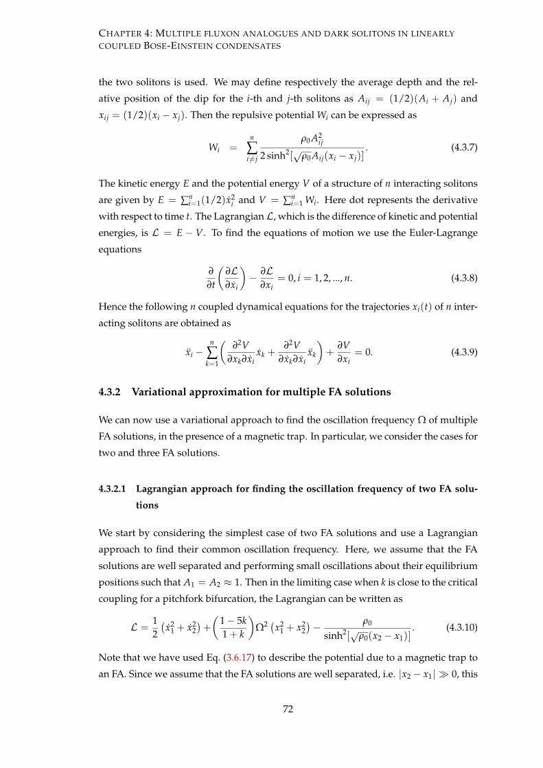
CHAPTER 4: MULTIPLE FLUXON ANALOGUES AND DARK SOLITONS IN LINEARLY
COUPLED BOSE-EINSTEIN CONDENSATES
the two solitons is used. We may define respectively the average depth and the rel-
ative position of the dip for the i-th and j-th solitons as Aij = (1/2)(Ai + Aj) and
xij = (1/2)(xi − xj). Then the repulsive potential Wi can be expressed as
Wi =n
∑i =j
ρ0A2ij
2 sinh2[√
ρ0 Aij(xi − xj)]. (4.3.7)
The kinetic energy E and the potential energy V of a structure of n interacting solitons
are given by E = ∑ni=1(1/2)x2
i and V = ∑ni=1 Wi. Here dot represents the derivative
with respect to time t. The Lagrangian L, which is the difference of kinetic and potential
energies, is L = E − V. To find the equations of motion we use the Euler-Lagrange
equations
∂
∂t
(∂L∂xi
)− ∂L
∂xi= 0, i = 1, 2, ..., n. (4.3.8)
Hence the following n coupled dynamical equations for the trajectories xi(t) of n inter-
acting solitons are obtained as
xi −n
∑k=1
(∂2V
∂xk∂xixk +
∂2V∂xk∂xi
xk
)+
∂V∂xi
= 0. (4.3.9)
4.3.2 Variational approximation for multiple FA solutions
We can now use a variational approach to find the oscillation frequency Ω of multiple
FA solutions, in the presence of a magnetic trap. In particular, we consider the cases for
two and three FA solutions.
4.3.2.1 Lagrangian approach for finding the oscillation frequency of two FA solu-
tions
We start by considering the simplest case of two FA solutions and use a Lagrangian
approach to find their common oscillation frequency. Here, we assume that the FA
solutions are well separated and performing small oscillations about their equilibrium
positions such that A1 = A2 ≈ 1. Then in the limiting case when k is close to the critical
coupling for a pitchfork bifurcation, the Lagrangian can be written as
L =12(
x21 + x2
2)+
(1 − 5k1 + k
)Ω2 (x2
1 + x22)− ρ0
sinh2[√
ρ0(x2 − x1)]. (4.3.10)
Note that we have used Eq. (3.6.17) to describe the potential due to a magnetic trap to
an FA. Since we assume that the FA solutions are well separated, i.e. |x2 − x1| ≫ 0, this
72

CHAPTER 4: MULTIPLE FLUXON ANALOGUES AND DARK SOLITONS IN LINEARLY
COUPLED BOSE-EINSTEIN CONDENSATES
implies that e−√
ρ0(x2−x1) approaches zero. Hence, Eq. (4.3.10) can be approximated by
L =12(
x21 + x2
2)+
(1 − 5k1 + k
)Ω2 (x2
1 + x22)− 4ρ0e−2
√ρ0(x2−x1).
Using Eq. (4.3.8), we then have the following system of governing equations
x1 = −8ρ320 e−2
√ρ0(x2−x1) + 2
(1 − 5k1 + k
)Ω2x1, (4.3.11)
x2 = 8ρ320 e−2
√ρ0(x2−x1) + 2
(1 − 5k1 + k
)Ω2x2. (4.3.12)
In order to find the fixed points of this system, we set x1 = 0 = x2. On adding the
resulting equations one can easily see that both fixed points x1 and x2 are additive
inverse of each other i.e. x1 = −x2 = x (say), from which we obtain a single nonlinear
algebraic equation which is
8ρ320 e4
√ρ0 x − 2
(1 − 5k1 + k
)Ω2x = 0. (4.3.13)
This equation could to be solved numerically to find the values of x corresponding to
different values of k.
Now let δ1 and δ2 be small perturbations in x1 and x2 and X1 = x + δ1(x1, t), X2 =
−x + δ2(x2, t) be the solutions of Eq. (4.3.11) and Eq. (4.3.12), respectively. Substituting
these solutions into Eq. (4.3.11), we obtain
δ1 = −8ρ320 e4
√ρ0 xe−2
√ρ0(δ2−δ1) + 2
(1 − 5k1 + k
)Ω2(x + δ1).
Using Taylor series expansion of e−2√
ρ0(δ2−δ1) in the first term on the right hand side
yields
δ1 = −8ρ320 e4
√ρ0 x[1 − 2
√ρ0(δ2 − δ1)] + 2
(1 − 5k1 + k
)Ω2(x + δ1).
Using Eq. (4.3.13), the above equation reduces to
δ1 = 16ρ20e4
√ρ0 x(δ2 − δ1) + 2
(1 − 5k1 + k
)Ω2δ1. (4.3.14)
Similarly from Eq. (4.3.12) we obtain
δ2 = −16ρ20e4
√ρ0 x(δ2 − δ1) + 2
(1 − 5k1 + k
)Ω2δ2. (4.3.15)
Now let ω be the common oscillation frequency of FA solutions, then we can write
δ1 = γ1eiωt and δ2 = γ2eiωt. Substituting these values into Eq. (4.3.14) and Eq. (4.3.15),
we obtain
− ω2γ1 = 16ρ20e4
√ρ0 x(γ2 − γ1) + 2
(1 − 5k1 + k
)Ω2γ1, (4.3.16)
−ω2γ2 = −16ρ20e4
√ρ0 x(γ2 − γ1) + 2
(1 − 5k1 + k
)Ω2γ2. (4.3.17)
73
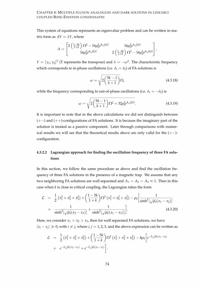
CHAPTER 4: MULTIPLE FLUXON ANALOGUES AND DARK SOLITONS IN LINEARLY
COUPLED BOSE-EINSTEIN CONDENSATES
This system of equations represents an eigenvalue problem and can be written in ma-
trix form as AY = λY, where
A =
2(
1−5k1+k
)Ω2 − 16ρ2
0e4√
ρ0 x 16ρ20e4
√ρ0 x
16ρ20e4
√ρ0 x 2
(1−5k1+k
)Ω2 − 16ρ2
0e4√
ρ0 x
,
Y = [γ1, γ2]T (T represents the transpose) and λ = −ω2. The characteristic frequency
which corresponds to in-phase oscillations (i.e. δ1 = δ2) of FA solutions is
ω =
√2(
5k − 1k + 1
)Ω, (4.3.18)
while the frequency corresponding to out-of-phase oscillations (i.e. δ1 = −δ2) is
ω =
√2(
5k − 1k + 1
)Ω2 + 32ρ2
0e4√
ρ0 x. (4.3.19)
It is important to note that in the above calculations we did not distinguish between
(+−) and (++)-configurations of FA solutions. It is because the imaginary part of the
solution is treated as a passive component. Later through comparisons with numer-
ical results we will see that the theoretical results above are only valid for the (+−)-
configuration.
4.3.2.2 Lagrangian approach for finding the oscillation frequency of three FA solu-
tions
In this section, we follow the same procedure as above and find the oscillation fre-
quency of three FA solutions in the presence of a magnetic trap. We assume that any
two neighboring FA solutions are well separated and A1 = A2 = A3 ≈ 1. Then in this
case when k is close to critical coupling, the Lagrangian takes the form
L =12(
x21 + x2
2 + x23)+
(1 − 5k1 + k
)Ω2 (x2
1 + x22 + x2
3)− ρ0
[1
sinh2[√
ρ0(x1 − x2)]
+1
sinh2[√
ρ0(x2 − x3)]+
1sinh2[
√ρ0(x1 − x3)]
]. (4.3.20)
Here, we consider x1 > x2 > x3, then for well separated FA solutions, we have
|xi − xj| ≫ 0, with i = j, where i, j = 1, 2, 3, and the above expression can be written as
L =12(
x21 + x2
2 + x23)+
(1 − 5k1 + k
)Ω2 (x2
1 + x22 + x2
3)− 4ρ0
[e−2
√ρ0(x1−x2)
+ e−2√
ρ0(x2−x3) + e−2√
ρ0(x1−x3)
].
74

CHAPTER 4: MULTIPLE FLUXON ANALOGUES AND DARK SOLITONS IN LINEARLY
COUPLED BOSE-EINSTEIN CONDENSATES
The Euler-Lagrange equations corresponding to the above Lagrangian are
x1 = 2(
1 − 5k1 + k
)Ω2x1 + 8ρ
320
[e−2
√ρ0(x1−x2) − e−2
√ρ0(x1−x3)
], (4.3.21)
x2 = 2(
1 − 5k1 + k
)Ω2x2 − 8ρ
320
[e−2
√ρ0(x1−x2) − e−2
√ρ0(x2−x3)
], (4.3.22)
x3 = 2(
1 − 5k1 + k
)Ω2x3 − 8ρ
320
[e−2
√ρ0(x2−x3) − e−2
√ρ0(x1−x3)
]. (4.3.23)
It is easy to see that the system of Eq. (4.3.21), Eq. (4.3.22), Eq. (4.3.23) has a fixed point
solution given by x1 = −x3 = x and x2 = 0. Consequently, we obtain
2(
1 − 5k1 + k
)Ω2 x + 8ρ
320
[e−2
√ρ0 x − e−4
√ρ0 x]= 0, (4.3.24)
This equation can be solved numerically to obtain the values of x for different values
of k.
Next, suppose that the small perturbations in the equilibrium positions x1, x2 and x3
are δ1, δ2 and δ3 respectively, then from Eq. (4.3.21), Eq. (4.3.22) and Eq. (4.3.23), we
derive the following perturbation equations
δ1 = 2(
1 − 5k1 + k
)Ω2δ1 − 16ρ2
0e−2√
ρ0 x(δ1 − δ2) + 16ρ20e−4
√ρ0 x(δ1 − δ3), (4.3.25)
δ2 = 2(
1 − 5k1 + k
)Ω2δ2 + 16ρ2
0e−2√
ρ0 x (δ1 − 2δ2 + δ3) , (4.3.26)
δ3 = 2(
1 − 5k1 + k
)Ω2δ3 + 16ρ2
0e−2√
ρ0 x(δ2 − δ3)− 16ρ20e−4
√ρ0 x(δ1 − δ3). (4.3.27)
Equations (4.3.25)-(4.3.27) are linear in δ1, δ2 and δ3, we consider solutions of the form
δ1 = γ1eiωt and δ2 = γ2eiωt and δ3 = γ3eiωt, where as before, ω is the common oscil-
lation frequency of three FA solutions. Inserting these values into Eqs. (4.3.25)-(4.3.27),
we obtain the following equations of motion
− ω2γ1 = 2(
1 − 5k1 + k
)Ω2γ1 − 16ρ2
0e−2√
ρ0 x(γ1 − γ2)
+ 16ρ20e−4
√ρ0 x(γ1 − γ3), (4.3.28)
−ω2γ2 = 2(
1 − 5k1 + k
)Ω2γ2 + 16ρ2
0e−2√
ρ0 x (γ1 − 2γ2 + γ3) , (4.3.29)
−ω2γ3 = 2(
1 − 5k1 + k
)Ω2γ3 + 16ρ2
0e−2√
ρ0 x(γ2 − γ3)
− 16ρ20e−4
√ρ0 x(γ1 − γ3). (4.3.30)
These equations of motion correspond to an eigenvalue problem AY = λY, where
A =
a11 a12 a13
a21 a22 a23
a31 a32 a33
,
75
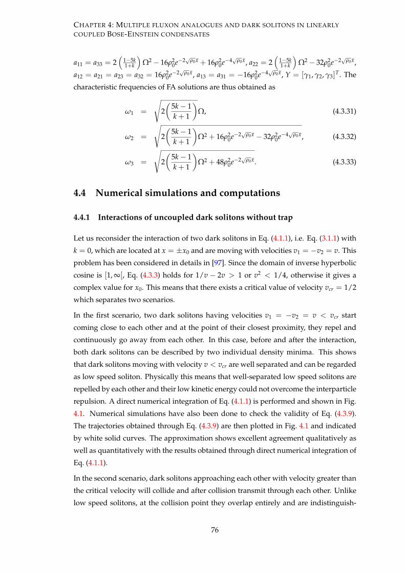
CHAPTER 4: MULTIPLE FLUXON ANALOGUES AND DARK SOLITONS IN LINEARLY
COUPLED BOSE-EINSTEIN CONDENSATES
a11 = a33 = 2(
1−5k1+k
)Ω2 − 16ρ2
0e−2√
ρ0 x + 16ρ20e−4
√ρ0 x, a22 = 2
(1−5k1+k
)Ω2 − 32ρ2
0e−2√
ρ0 x,
a12 = a21 = a23 = a32 = 16ρ20e−2
√ρ0 x, a13 = a31 = −16ρ2
0e−4√
ρ0 x, Y = [γ1, γ2, γ3]T. The
characteristic frequencies of FA solutions are thus obtained as
ω1 =
√2(
5k − 1k + 1
)Ω, (4.3.31)
ω2 =
√2(
5k − 1k + 1
)Ω2 + 16ρ2
0e−2√
ρ0 x − 32ρ20e−4
√ρ0 x, (4.3.32)
ω3 =
√2(
5k − 1k + 1
)Ω2 + 48ρ2
0e−2√
ρ0 x. (4.3.33)
4.4 Numerical simulations and computations
4.4.1 Interactions of uncoupled dark solitons without trap
Let us reconsider the interaction of two dark solitons in Eq. (4.1.1), i.e. Eq. (3.1.1) with
k = 0, which are located at x = ±x0 and are moving with velocities v1 = −v2 = v. This
problem has been considered in details in [97]. Since the domain of inverse hyperbolic
cosine is [1, ∞[, Eq. (4.3.3) holds for 1/v − 2v > 1 or v2 < 1/4, otherwise it gives a
complex value for x0. This means that there exists a critical value of velocity vcr = 1/2
which separates two scenarios.
In the first scenario, two dark solitons having velocities v1 = −v2 = v < vcr start
coming close to each other and at the point of their closest proximity, they repel and
continuously go away from each other. In this case, before and after the interaction,
both dark solitons can be described by two individual density minima. This shows
that dark solitons moving with velocity v < vcr are well separated and can be regarded
as low speed soliton. Physically this means that well-separated low speed solitons are
repelled by each other and their low kinetic energy could not overcome the interparticle
repulsion. A direct numerical integration of Eq. (4.1.1) is performed and shown in Fig.
4.1. Numerical simulations have also been done to check the validity of Eq. (4.3.9).
The trajectories obtained through Eq. (4.3.9) are then plotted in Fig. 4.1 and indicated
by white solid curves. The approximation shows excellent agreement qualitatively as
well as quantitatively with the results obtained through direct numerical integration of
Eq. (4.1.1).
In the second scenario, dark solitons approaching each other with velocity greater than
the critical velocity will collide and after collision transmit through each other. Unlike
low speed solitons, at the collision point they overlap entirely and are indistinguish-
76

CHAPTER 4: MULTIPLE FLUXON ANALOGUES AND DARK SOLITONS IN LINEARLY
COUPLED BOSE-EINSTEIN CONDENSATES
x
t
−20 −10 0 10 20
20
40
60
80
100
120
0.2
0.4
0.6
0.8
1
Figure 4.1: Numerical evolutions of interaction of two dark solitons. The solitons are
moving with velocities v1 = −v2 = 0.1. The interparticle repulsion is
dominant over the kinetic energies of solitons and solitons are going away
from each other after interaction. The white solid curves are simulations
of trajectories of solutions obtained through Eq. (4.3.9). Note that an exact
analytic solution is given by (4.1.2).
able. Physically this means that due to the high velocity, their kinetic energy defeats
the interparticle repulsion. This situation is shown in Fig. 4.2. Even though this case
is beyond the particle-like approximation, we show in Fig. 4.2 that Eq. (4.3.9) can still
provide an approximate trajectory of the soliton collision.
In the above discussion, we only considered the symmetric case where solitons collide
with the same absolute velocity. Let us now consider the asymmetric case. In this case,
a dark soliton moving with velocity v will interact with a static dark soliton. At the
interaction point, the static soliton is repelled by the travelling soliton. The energy pos-
sessed by the moving soliton is used to push the static soliton away from the original
position. The travelling soliton transfers all its kinetic energy to the static soliton and
becomes stationary after collision as shown in Fig. 4.3. The white solid lines in this
figure depict the trajectories obtained through the numerical integration of Eq. (4.3.9).
4.4.2 Interaction of dark solitons in coupled NLS equations without trap
Next, we consider the case k = 0. Let us first consider the symmetric case in which
a pair of coupled dark solitons interact with each other. The interaction scenarios for
coupled dark solitons are almost similar to the scenarios for the uncoupled dark soli-
tons in the previous section. The scenario for slow moving solitons is presented in Fig.
77

CHAPTER 4: MULTIPLE FLUXON ANALOGUES AND DARK SOLITONS IN LINEARLY
COUPLED BOSE-EINSTEIN CONDENSATES
x
t
−20 −10 0 10 20
5
10
15
20
25
30
0.3
0.4
0.5
0.6
0.7
0.8
0.9
1
Figure 4.2: Numerical evolutions of interaction of two dark solitons. The solitons are
moving with velocities v1 = −v2 = 0.6. The interparticle repulsion is sup-
pressed by the kinetic energies of the solitons and they transmit through
each other at the interacting point. The white solid curves are simulations
of trajectories of solutions obtained through Eq. (4.3.9). The exact analytic
solution is given by (4.1.2).
x
t
−20 −10 0 10 20
5
10
15
20
25
30
0.2
0.4
0.6
0.8
1
Figure 4.3: Numerical evolutions of interaction of two dark solitons. One of the soli-
tons is static and the other is moving with velocity v = 0.5. After interac-
tion, the travelling soliton becomes stationary and the static soliton starts
moving with the velocity of the other soliton. The white solid curves are
simulations of trajectories of solutions obtained through Eq. (4.3.9).
78
CHAPTER 4: MULTIPLE FLUXON ANALOGUES AND DARK SOLITONS IN LINEARLY
COUPLED BOSE-EINSTEIN CONDENSATES
4.4, where we can see that both coupled solitons are repelling each other and remain
well separated for all time t. The only difference from the uncoupled case is that there
is radiation emerging after interaction which was not seen in the uncoupled case. The
reason for the emergence of this radiation is because the system is non-integrable. Also
after a particular time the coupled dark solitons break up because they are unstable
for the parameter values used for the interaction. Since a travelling uncoupled dark
soliton is stable for all values of velocity, no radiation or break up could be seen. In the
interaction scenario of the fast moving coupled solitons, they transmit through each
other. Like in the uncoupled case, their high kinetic energy overcomes the interparticle
repulsion as shown in Fig. 4.5. In an asymmetric interaction when one of the coupled
dark solitons is static while the other is moving with some non-zero velocity v, the
interaction scenario is similar to that of the uncoupled case and is shown in Fig. 4.6.
The trajectories of dips obtained by doing numerical simulations of Eq. (4.3.9) are com-
pared with the trajectories found through direct numerical integration of Eq. (3.1.1).
The white solid curves in Figs. 4.4-4.6 are the approximations obtained through Eq.
(4.3.9) showing excellent agreement.
We also consider the interaction of three coupled dark solitons when one of the solitons
is static and the other two are moving with opposite velocities. The scenarios resemble
to that of the interaction scenarios of two solitons as above. The interaction of slow
moving solitons is shown in Fig. 4.7. The travelling solitons are repelling each other
without affecting the static soliton in the middle. However, the break up could be seen
due to the instability of the travelling dark solitons. The interaction of the fast moving
solitons is presented in Fig. 4.8, where the moving solitons transmit through each other
leaving the stationary dark soliton at rest.
4.4.3 Interaction of FA solutions in the absence of a magnetic trap
In this section, we will consider symmetric as well as asymmetric interactions of two
FA solutions. An FA solution moving with velocity v corresponding to a particular
value of k is shown in Fig. 3.21. We use a numerically obtained FA solution to construct
a collision of two FA solutions. Since FA are coupled solutions which consist of Ψ1 and
Ψ2, there are two possibilities to connect two FA solutions. In the first possibility, Ψ1
and Ψ2 of the first FA are connected respectively to Ψ1 and Ψ2 of the second FA solution.
In the second possibility, Ψ1 and Ψ2 of the first FA are connected respectively to Ψ2 and
Ψ1 of the second FA solution. The combined pictures for both possibilities are shown
in Fig. 4.9. From the symmetry of the imaginary parts, we refer to the first possibility
as an odd symmetric interaction or (+−)-configuration and the second possibility as
79

CHAPTER 4: MULTIPLE FLUXON ANALOGUES AND DARK SOLITONS IN LINEARLY
COUPLED BOSE-EINSTEIN CONDENSATES
x
t
−20 0 20
20
40
60
80
100
120
140
x
t
−20 0 20
20
40
60
80
100
120
140
0.2
0.4
0.6
0.8
1
0.2
0.4
0.6
0.8
1
Figure 4.4: Numerical evolutions of interaction of two coupled dark solitons for k =
0.1. The solitons are moving with velocities v1 = −v2 = 0.2. The interpar-
ticle repulsion is dominant over the kinetic energies and the solitons are
going away from each other after interaction. Due to an instability, they
break down at approximately t = 120. The white solid curves are simula-
tions of trajectories of solutions obtained through Eq. (4.3.9).
x
t
−20 0 20
5
10
15
20
25
30
x
t
−20 0 20
5
10
15
20
25
30
0.2
0.3
0.4
0.5
0.6
0.7
0.8
0.9
1
0.2
0.3
0.4
0.5
0.6
0.7
0.8
0.9
1
Figure 4.5: Numerical evolutions of interaction of two coupled dark solitons for k =
0.1. The solitons are moving with velocities v1 = −v2 = 0.6. The in-
terparticle repulsion is suppressed by the kinetic energies of the solitons
and they transmit through each other at the interacting point. The white
solid curves are simulations of trajectories of solutions obtained through
Eq. (4.3.9).
80

CHAPTER 4: MULTIPLE FLUXON ANALOGUES AND DARK SOLITONS IN LINEARLY
COUPLED BOSE-EINSTEIN CONDENSATES
x
t
−20 0 20
5
10
15
20
25
30
x
t
−20 0 20
5
10
15
20
25
30
0.2
0.4
0.6
0.8
1
0.2
0.4
0.6
0.8
1
Figure 4.6: Numerical evolutions of interaction of two coupled dark solitons for k =
0.1. One of the coupled solitons is static and the other is moving with
velocity v = 0.5. The white solid curves are simulations of trajectories of
solutions obtained through Eq. (4.3.9).
x
t
−20 0 20
20
40
60
80
100
120
140
x
t
−20 0 20
20
40
60
80
100
120
140
0.2
0.4
0.6
0.8
1
1.2
0.2
0.4
0.6
0.8
1
1.2
Figure 4.7: Numerical evolutions of collision of three coupled dark solitons for k =
0.1. Two solitons are moving with velocities v1 = −v3 = 0.2 and the soli-
ton between these moving solitons is at rest, i.e. v2 = 0. The interparticle
repulsion is dominant over the kinetic energies and the solitons are going
away from each other after interaction. The break up is due to the instabil-
ity of the travelling dark solitons.
81

CHAPTER 4: MULTIPLE FLUXON ANALOGUES AND DARK SOLITONS IN LINEARLY
COUPLED BOSE-EINSTEIN CONDENSATES
x
t
−20 0 20
5
10
15
20
25
30
35
40
45
50
x
t
−20 0 20
5
10
15
20
25
30
35
40
45
50
0.2
0.4
0.6
0.8
1
0.2
0.4
0.6
0.8
1
Figure 4.8: Numerical evolutions of collision of three coupled dark solitons for k =
0.1. The solitons are moving with velocities v1 = −v2 = 0.6 and v2 = 0.
The interparticle repulsion is suppressed by the kinetic energies of the soli-
tons and the moving solitons transmit through each other at the interacting
point leaving the static soliton undisturbed.
an even symmetric interaction or (++)-configuration.
First, we discuss the odd symmetric interaction. In this case, two FA solutions initially
localized at x = ±x0 move with opposite velocities. Shown in Fig. 4.10 is the inter-
action of relatively slow moving FA solutions. Both FA solutions can be characterized
by an individual density minimum before and after collision while at the interacting
point they exhibit a single nonzero density minima. Both FA solutions show attraction
towards each other at the interacting point which results in the deflection of positions
of dips of both solutions. Radiation emerges and phase shift is induced due to collision.
Fig. 4.11 depicts an interaction of relatively high speed FA solutions. Neither of the FA
solutions show any resistance during collision. Due to their high kinetic energies, both
FA solutions pass through each other without shifting the phase and without showing
any deflection in the trajectories of their dips.
Next, we consider the even symmetric interaction. An interaction of extremely slow
moving FA solutions is displayed in Fig. 4.12. The FA solutions come close to each
other, but at the point of their closest proximity, they repel each other. Both the so-
lutions can be identified by two individual density minima before and after the inter-
action as well as at the point of interaction. Another output from the interaction of
two FA solutions moving with relatively slow velocities is shown in Fig. 4.13. In this
scenario, the solitons merge and form a breather similar to that reported in [133] in a
82

CHAPTER 4: MULTIPLE FLUXON ANALOGUES AND DARK SOLITONS IN LINEARLY
COUPLED BOSE-EINSTEIN CONDENSATES
parametrically driven Schrödinger equation. Radiation emerging after the collision is
clear. Shown in Fig. 4.14 is the collision of FA solution moving with relatively high
velocities. The FA solutions collide with each other and become indistinguishable at
the interacting point.
Finally, we consider asymmetric interactions of two FA solutions. We show in Fig. 4.15
an odd interaction of a relatively slow moving FA with a static FA. The travelling FA
pushes the static FA away from the interacting point. This means that the travelling
FA transfers all its kinetic energy to the static FA. Due to collision, radiation appears.
In Fig. 4.16 we show an interaction of a relatively fast moving FA solution with a static
FA solution, where we obtain a similar behavior as before. Even interactions of a slow
and a fast moving FA with a static FA are shown in Fig. 4.17 and Fig. 4.18, respectively.
From Figs. 4.15-4.18, one can conclude that the collisions of a moving and a static FA
are strongly inelastic. The radiation after the collision is so pronounced that it can be
difficult to identify the outputs of the collisions.
The interactions of three FA solutions when one of them is at rest and the other two are
moving is considered as well. In Fig. 4.19, we present the interaction of relatively slow
moving FA solutions, where one of the travelling FA solutions transmits through the
other FA solutions with a small shift in its trajectory. The other two FA solutions are
indistinguishable after the collision. The interaction of the fast moving FA solutions is
depicted in Fig. 4.20. Here, the fast moving FA solutions collide with each other and
are indistinguishable.
4.4.4 Stationary multiple FA solutions and dark solitons in the presence of
magnetic trap
In this section, we will consider the existence, stability and time-dynamics of multiple
FA solutions and dark solitons in the coupled NLS Eq. (3.1.1) in the presence of a mag-
netic trap. In particular, we consider stationary solutions of the governing equations.
To seek static solutions in the time-independent framework of Eq. (3.1.1), we use a
Newton-Raphson continuation method. The spatial second order derivative is approx-
imated using central finite differences with three-point or five-point stencils. At the
computational boundaries, we use Neumann boundary conditions. In all the calcula-
tions, the grid spacing ∆x = 0.2 or smaller. Numerical linear stability analysis of a
solution Ψ(0)j (x) is then performed by looking for perturbed solutions of the form
Ψj = Ψ(0)j (x) + ϵ[aj(x) eiλt + b∗j (x) e−iλ∗t], j = 1, 2.
Substituting the ansatz into the governing Eq. (3.1.1) and keeping the linear terms in
83

CHAPTER 4: MULTIPLE FLUXON ANALOGUES AND DARK SOLITONS IN LINEARLY
COUPLED BOSE-EINSTEIN CONDENSATES
−40 −20 0 20 40−1
0
1
x
Ψ1
−40 −20 0 20 40−1
0
1
x
Ψ2
(a)
−40 −20 0 20 40−1
0
1
x
Ψ1
−40 −20 0 20 40−1
0
1
x
Ψ2
(b)
Figure 4.9: Profiles of an initial condition representing two coupled FA solutions trav-
elling with velocities v1 = −v2 = 0.2 corresponding to k = 0.1. The fig-
ure in the upper panel represents the odd interaction referred to as (+−)-
configuration, while figure in the lower panel is the even interaction and
referred to as (++)-configuration of FA solution.
84

CHAPTER 4: MULTIPLE FLUXON ANALOGUES AND DARK SOLITONS IN LINEARLY
COUPLED BOSE-EINSTEIN CONDENSATES
x
t
−20 0 20
10
20
30
40
50
60
xt
−20 0 20
10
20
30
40
50
60
0.2
0.4
0.6
0.8
1
0.2
0.4
0.6
0.8
1
Figure 4.10: As Fig. 4.1, but for the odd symmetric collision of FA solutions for v = 0.2
and k = 0.1.
x
t
−20 0 20
5
10
15
20
25
30
x
t
−20 0 20
5
10
15
20
25
30
0.3
0.4
0.5
0.6
0.7
0.8
0.9
1
0.3
0.4
0.5
0.6
0.7
0.8
0.9
1
Figure 4.11: As Fig. 4.1, but for the odd symmetric collision of FA solutions for v = 0.6
and k = 0.1.
85

CHAPTER 4: MULTIPLE FLUXON ANALOGUES AND DARK SOLITONS IN LINEARLY
COUPLED BOSE-EINSTEIN CONDENSATES
x
t
−20 0 20
10
20
30
40
50
60
70
80
xt
−20 0 20
10
20
30
40
50
60
70
80
0.88
0.9
0.92
0.94
0.96
0.98
1
1.02
1.04
0.4
0.5
0.6
0.7
0.8
0.9
1
Figure 4.12: As Fig. 4.1, but the even symmetric collision of FA solutions for v = 0.1
and k = 0.1.
x
t
−40 −20 0 20 40
10
20
30
40
50
60
x
t
−40 −20 0 20 40
10
20
30
40
50
60
0.5
0.6
0.7
0.8
0.9
1
1.1
1.2
1.3
0.2
0.4
0.6
0.8
1
1.2
Figure 4.13: As Fig. 4.1, but the even symmetric collision of FA solutions for v = 0.2
and k = 0.1.
86

CHAPTER 4: MULTIPLE FLUXON ANALOGUES AND DARK SOLITONS IN LINEARLY
COUPLED BOSE-EINSTEIN CONDENSATES
x
t
−20 0 20
5
10
15
20
25
30
xt
−20 0 20
5
10
15
20
25
30
0.5
0.6
0.7
0.8
0.9
1
0.2
0.4
0.6
0.8
1
Figure 4.14: As Fig. 4.1, but the even symmetric collision of FA solutions for v = 0.6
and k = 0.1.
x
t
−20 0 20
10
20
30
40
50
60
x
t
−20 0 20
10
20
30
40
50
60
0.5
0.6
0.7
0.8
0.9
1
1.1
0.2
0.4
0.6
0.8
1
Figure 4.15: Numerical evolutions of the odd symmetric collisions of two FA solutions
when one of them is static while the other is moving with velocity v = 0.2
and k = 0.1.
87

CHAPTER 4: MULTIPLE FLUXON ANALOGUES AND DARK SOLITONS IN LINEARLY
COUPLED BOSE-EINSTEIN CONDENSATES
x
t
−20 0 20
5
10
15
20
25
30
xt
−20 0 20
5
10
15
20
25
30
0.5
0.6
0.7
0.8
0.9
1
1.1
0.4
0.5
0.6
0.7
0.8
0.9
1
1.1
Figure 4.16: Numerical evolutions of the odd symmetric collisions of two FA solutions
when one of them is static while the other is moving with velocity v = 0.6
and k = 0.1.
x
t
−20 0 20
10
20
30
40
50
60
x
t
−20 0 20
10
20
30
40
50
60
0.2
0.4
0.6
0.8
1
0.2
0.4
0.6
0.8
1
Figure 4.17: As Fig. 4.15, but the even symmetric collision of FA solutions for v = 0.2
and k = 0.1.
88
CHAPTER 4: MULTIPLE FLUXON ANALOGUES AND DARK SOLITONS IN LINEARLY
COUPLED BOSE-EINSTEIN CONDENSATES
x
t
−20 0 20
5
10
15
20
25
30
xt
−20 0 20
5
10
15
20
25
30
0.2
0.4
0.6
0.8
1
1.2
0.2
0.4
0.6
0.8
1
1.2
Figure 4.18: As Fig. 4.15, but the even symmetric collision of FA solutions for v = 0.6
and k = 0.1.
x
t
−20 0 20
10
20
30
40
50
x
t
−20 0 20
10
20
30
40
50
0.2
0.4
0.6
0.8
1
1.2
0.2
0.4
0.6
0.8
1
1.2
Figure 4.19: Numerical evolutions of collision of three FA solutions for k = 0.1. Two
FA solutions are moving with velocities v1 = −v3 = 0.2 and the FA solu-
tion in the middle is at rest.
89

CHAPTER 4: MULTIPLE FLUXON ANALOGUES AND DARK SOLITONS IN LINEARLY
COUPLED BOSE-EINSTEIN CONDENSATES
x
t
−20 0 20
5
10
15
20
25
30
x
t
−20 0 20
5
10
15
20
25
30
0.2
0.4
0.6
0.8
1
1.2
0.2
0.4
0.6
0.8
1
1.2
Figure 4.20: Numerical evolutions of collision of three FA solutions for k = 0.1. Two
FA solutions are moving with velocities v1 = −v3 = 0.6 and the other one
is at rest. The FA solutions are indistinguishable after the interaction.
ϵ, one will obtain a linear eigenvalue problem for the stability of Ψ(0)j . The ensuing
eigenvalue problem is then discretized using a similar finite difference scheme as above
and solved numerically for the eigenfrequency λ and corresponding eigenfunctions aj
and bj. It is then clear that Ψ(0)j (x) is a stable solution if the imaginary parts of all the
eigenvalues vanish, i.e. Im(λ) = 0.
4.4.4.1 (+−)-configuration of FA
First, we consider the (+−)-configuration of FA solutions of Eq. (3.1.1), which is shown
in Fig. 4.21. The amplitude of the imaginary parts of the solution reduces with k and
ultimately become zero at a critical value kce, when we obtain coupled dark solitons.
The imaginary parts remain zero for all values of k greater than or equal to kce.
We have calculated the existence and stability of FA solutions for different non-zero val-
ues of trapping parameter Ω. The critical value kce for which this FA solution changes
into dark soliton decreases with the increment of Ω and is depicted in Fig. 4.22. The
conversion of FA into coupled dark solitons for Ω = 0.1 is shown in Fig. 4.23. The
variation in the value of Ω also affects the stability of the solution. The critical coupling
kcs where the solution becomes stable increases with Ω as shown in Fig. 4.24. In this
case, the value of kcs always remains greater than its corresponding value of kce. This
shows that the (+−)-configuration of FA solution is completely unstable for all values
of k where it exists. We note that the value of kcs corresponding to a specific value of Ω
90

CHAPTER 4: MULTIPLE FLUXON ANALOGUES AND DARK SOLITONS IN LINEARLY
COUPLED BOSE-EINSTEIN CONDENSATES
−40 −20 0 20 40−1
0
1
2
xΨ
1
−40 −20 0 20 40−1
0
1
2
x
Ψ2
Figure 4.21: Numerically obtained multiple FA with a (+−)-configuration for Ω =
0.1, ρ0 = 1, k = 0.2.
is actually the critical value for dark soliton at which it attains stability. The eigenvalue
structure of FA for a specific value of Ω is displayed in Fig. 4.25 showing that most of
the eigenvalues are real as they are lying on the horizontal axis, while few of them are
complex. The most unstable eigenvalues are purely imaginary. The magnitude of the
most unstable pair of eigenvalues increases for all k ≤ kce and then decreases with k
and ultimately becomes zero at k = kcs. The stable eigenvalue structure for Ω = 0.1
is shown in Fig. 4.26 where all eigenvalues are lying on the horizontal axis showing
the stability of the solution. The stability curve is shown in Fig. 4.27 by a solid curve.
In the figure, we also present the stability curve of coupled dark solitons in dashed
line. At k = kce the solid and dashed curves meet. This corresponds to the situation
when FA turn into dark solitons, i.e. k = kce is a pitchfork bifurcation point. The dark
soliton becomes stable for k ≥ kcs. The dashed dotted curve shows the approximation
(4.3.19) obtained through a variational approach for Ω = 0.1, where one can see that a
qualitatively good agreement is obtained.
In order to verify our results, we solve the time-dependent system (3.1.1) numerically
for the configuration of FA solutions above. For Ω = 0.1 and k = 0.2, the numerical
evolution of the unstable FA solutions represented by Ψ1 and Ψ2 is shown in Fig. 4.28.
Different from the collisions of two moving FA solutions with (+−)-configuration that
are attractive (see Figs. 4.10 and 4.11), the dynamics of unstable stationary FA solutions
in here is rather repulsive. This can be seen in Fig. 4.28 where at t ≈ 100, the FA
solutions are moving away from each other.
91
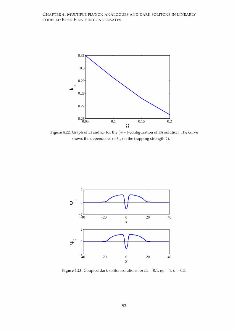
CHAPTER 4: MULTIPLE FLUXON ANALOGUES AND DARK SOLITONS IN LINEARLY
COUPLED BOSE-EINSTEIN CONDENSATES
0.05 0.1 0.15 0.20.26
0.27
0.28
0.29
0.3
0.31
Ω
k ce
Figure 4.22: Graph of Ω and kce for the (+−)-configuration of FA solution. The curve
shows the dependence of kce on the trapping strength Ω.
−40 −20 0 20 40−2
0
2
x
Ψ1
−40 −20 0 20 40−2
0
2
x
Ψ2
Figure 4.23: Coupled dark soliton solutions for Ω = 0.1, ρ0 = 1, k = 0.5.
92

CHAPTER 4: MULTIPLE FLUXON ANALOGUES AND DARK SOLITONS IN LINEARLY
COUPLED BOSE-EINSTEIN CONDENSATES
0.05 0.1 0.15 0.20.36
0.37
0.38
0.39
0.4
0.41
0.42
0.43
Ω
k cs
Figure 4.24: Graph of Ω and kcs for the (+−)-configuration of FA solution. The curve
shows the dependence of kcs on the trapping strength Ω.
−2 −1 0 1 2−0.2
−0.15
−0.1
−0.05
0
0.05
0.1
0.15
Re(λ)
Im(λ
)
Figure 4.25: The eigenvalue structure of the soliton in Fig. 4.21 in the complex plane.
93

CHAPTER 4: MULTIPLE FLUXON ANALOGUES AND DARK SOLITONS IN LINEARLY
COUPLED BOSE-EINSTEIN CONDENSATES
−10 −5 0 5 10−2
−1.5
−1
−0.5
0
0.5
1
1.5
2x 10
−9
Re(λ)
Im(λ
)
Figure 4.26: The spectrum of eigenvalues in the middle for Ω = 0.1 and k = 0.5 show-
ing the stability of the solution shown in Fig. 4.23.
0.1 0.2 0.3 0.4 0.50
0.05
0.1
0.15
0.2
0.25
0.3
0.35
0.4
k
Max
(Im
(λ))
Figure 4.27: The graph of k and the maximum imaginary parts of eigenvalues for
Ω = 0.1. The solid and dashed curves represent the trajectories of the
most unstable eigenvalue for FA and dark soliton as a function of k re-
spectively. The dash-dotted curve represents the approximation (4.3.19)
for the oscillation frequency of the (+−)-configuration of FA.
94

CHAPTER 4: MULTIPLE FLUXON ANALOGUES AND DARK SOLITONS IN LINEARLY
COUPLED BOSE-EINSTEIN CONDENSATES
t
x−20 0 20
50
100
150
200
t
x−20 0 20
50
100
150
200
0.2
0.4
0.6
0.8
1
1.2
0.2
0.4
0.6
0.8
1
1.2
Figure 4.28: Numerical evolution of the solution shown in Fig. 4.21 for Ω = 0.1 and
k = 0.2.
4.4.4.2 (++)-configuration of FA
Next, we consider FA solutions of Eq. (3.1.1) with (++)-configuration as shown in Fig.
4.29. Similarly to the (+−)-configuration, the imaginary parts of the solution reduce
to zero with k and at the critical value k = kce coupled dark solitons are obtained.
The critical value kce increases with Ω. The change in the value of Ω also changes
the critical value kcs for the stability of this solution. The stability curves for different
values of Ω are plotted in Fig. 4.31. We elaborate here, for example, for Ω = 0.1, the
(++)-configuration of FA solution is unstable for k < 0.16 due to two pairs of purely
imaginary eigenvalues. The solution remains stable up to k = 0.21, at which two pairs
of unstable eigenvalues emerge from the spectrum. The imaginary part of the unstable
eigenvalues becomes zero at k = 0.38 showing that the solution is stable for k ≥ 0.38.
The eigenvalues structure for Ω = 0.1 and k = 0.25 is shown in Fig. 4.30. Since this
solution changes into a dark soliton at k = 0.38, so the dark soliton is unstable for
k < 0.38 but becomes stable for k ≥ 0.38. The stability curve for Ω = 0.1 is shown in
Fig. 4.31(b) by a solid line. The real part of the most unstable eigenvalue as a function
of k is displayed in the same figure by a dashed line. At k = kce, the (++)-configuration
in FA solutions merges with dark solitons, similarly to the case of (+−)-configuration
in a pitchfork bifurcation. Note that our analytical result (4.3.19) cannot be used to
approximate the instability of the (++)-configuration. It is because (4.3.19) only yields
purely imaginary eigenvalues while the instability of the solution here is oscillatory.
The results obtained for the (++)-configuration of FA solutions above are also verified
95

CHAPTER 4: MULTIPLE FLUXON ANALOGUES AND DARK SOLITONS IN LINEARLY
COUPLED BOSE-EINSTEIN CONDENSATES
−30 −20 −10 0 10 20 30−2
0
2
xΨ
1
−30 −20 −10 0 10 20 30−2
0
2
x
Ψ2
Figure 4.29: Numerically obtained FA for a (++)-configuration with Ω = 0.1, ρ0 = 1,
k = 0.25.
by direct numerical integration of the time-dependent system (3.1.1). A typical evolu-
tion of unstable FA solutions is shown in Fig. 4.32 for Ω = 0.1 and k = 0.25. In a similar
fashion as the (+−)-configuration (see Fig. 4.28), the FA solutions repel each other. One
difference between Fig. 4.28 and Fig. 4.32 is that in the latter case the break up is pre-
ceded by oscillations of the soliton pair. This is caused by the fact that the stability is
oscillatory.
4.4.4.3 (+−+)-configuration of FA
Now we analyze the (+−+)-configuration of FA solutions of Eq. (3.1.1) which is dis-
played in Fig. 4.33. The amplitude and width of the real parts of the solution increases
while the amplitude of the imaginary parts decreases with k and become zero at k = kce,
i.e. we obtain dark solitons as depicted in Fig. 4.34. The values of kce and kcs for dif-
ferent values of Ω are found. Similarly to the (+−)-configuration of FA solutions, kce
decreases and kcs increases with Ω. We also noticed that the critical value kce always
remains smaller than kcs corresponding to a particular value of Ω. This means that the
(+ − +)-configuration of FA solution is unstable for all values of k in its domain of
existence. The eigenvalues structure for a particular value of Ω is shown in Fig. 4.35.
The critical eigenvalue as a function of k is depicted in Fig. 4.36 by a solid curve. The
dotted curve in the same figure is the critical eigenvalue for dark solitons. The dotted
curve indicates the existence of dark solitons in the domain of existence of (+ − +)-
configuration of FA solutions. At k = kce, the FA bifurcates into a dark solitons as a
96

CHAPTER 4: MULTIPLE FLUXON ANALOGUES AND DARK SOLITONS IN LINEARLY
COUPLED BOSE-EINSTEIN CONDENSATES
−10 −5 0 5 10−0.03
−0.02
−0.01
0
0.01
0.02
0.03
Im(λ
)
Re(λ)Figure 4.30: The eigenvalue structure of the soliton in Fig. 4.29. All eigenvalues are
real except two pairs of eigenvalues, which are complex, indicating the
instability of the solution.
pitchfork bifurcation.
We then solve the time-dependent Eq. (3.1.1) numerically for the (+−+)-configuration
of FA solutions. The spatiotemporal contour plot for Ω = 0.1 and k = 0.1 is shown in
Fig. 4.37. One can see that the repulsion between the right and the middle solitons is
dominant over the repulsion between the middle and the left solitons. As a result, the
middle and the right solitons appear to oscillate and the whole structure break up.
4.4.4.4 (+++)-configuration of FA
Finally, we examine the (+ + +)-configuration of FA solution of Eq. (3.1.1) as shown
in Fig. 4.38. The variation in the profile of the solution is similar to the (+ − +)-
configuration of FA solution, i.e. at a critical value k = kce, we obtain a dark soliton
with a pitchfork bifurcation. Like the (++)-configuration of FA, both kce and kcs in-
creases with Ω. The unstable eigenvalues structure for Ω = 0.1 is presented in Fig.
4.39. The stability curves for different values of Ω are shown in Fig. 4.40. The contour
plot obtained on solving the time-dependent Eq. (3.1.1) is depicted in Fig. 4.41. Like
the (+−+)-configuration, the FA solutions herein repel each other which results in the
breakage of the structure.
97

CHAPTER 4: MULTIPLE FLUXON ANALOGUES AND DARK SOLITONS IN LINEARLY
COUPLED BOSE-EINSTEIN CONDENSATES
0.1 0.2 0.3 0.4 0.50
0.01
0.02
0.03
0.04
0.05
0.06
0.07
k
Max
(Im
(λ))
(a)
0.1 0.2 0.3 0.4 0.50
0.05
0.1
0.15
0.2
0.25
0.3
0.35
k
(b)
0.1 0.2 0.3 0.4 0.50
0.05
0.1
0.15
0.2
0.25
k
Max
(Im
(λ))
(c)
0.1 0.2 0.3 0.4 0.50
0.05
0.1
0.15
0.2
0.25
0.3
0.35
0.4
k
Max
(Im
(λ))
(d)
Figure 4.31: The trajectories of the most unstable eigenvalue λmax corresponding to
Ω = 0.05, 0.1, 0.15, 0.2 for FA solution with the (++)-configuration. In
(b), the imaginary part of λmax is represented by the solid curve. The
dashed line is the eigenvalue of coupled dark solitons (see Fig. 4.27). The
dash-dotted curve shows the real part of λmax indicating an oscillatory
instability when it is nonzero.
98
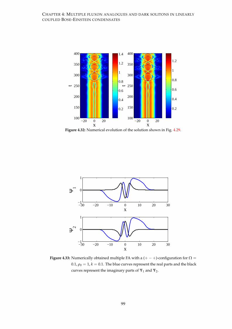
CHAPTER 4: MULTIPLE FLUXON ANALOGUES AND DARK SOLITONS IN LINEARLY
COUPLED BOSE-EINSTEIN CONDENSATES
x
t
−20 0 20100
150
200
250
300
350
400
xt
−20 0 20100
150
200
250
300
350
400
0.2
0.4
0.6
0.8
1
1.2
1.4
0.2
0.4
0.6
0.8
1
1.2
Figure 4.32: Numerical evolution of the solution shown in Fig. 4.29.
−30 −20 −10 0 10 20 30−1
0
1
x
Ψ1
−30 −20 −10 0 10 20 30−1
0
1
x
Ψ2
Figure 4.33: Numerically obtained multiple FA with a (+−+)-configuration for Ω =
0.1, ρ0 = 1, k = 0.1. The blue curves represent the real parts and the black
curves represent the imaginary parts of Ψ1 and Ψ2.
99

CHAPTER 4: MULTIPLE FLUXON ANALOGUES AND DARK SOLITONS IN LINEARLY
COUPLED BOSE-EINSTEIN CONDENSATES
−30 −20 −10 0 10 20 30−2
0
2
x
Ψ1
−30 −20 −10 0 10 20 30−2
0
2
x
Ψ2
Figure 4.34: Coupled dark soliton solutions for Ω = 0.1, ρ0 = 1, k = 0.5.
−10 −5 0 5 10−0.4
−0.3
−0.2
−0.1
0
0.1
0.2
0.3
Re(λ)
Im(λ
)
Figure 4.35: The eigenvalue structure of the (+−+)-configuration of FA in the com-
plex plane for Ω = 0.1, ρ0 = 1, k = 0.2.
100

CHAPTER 4: MULTIPLE FLUXON ANALOGUES AND DARK SOLITONS IN LINEARLY
COUPLED BOSE-EINSTEIN CONDENSATES
0.1 0.2 0.3 0.4 0.50
0.05
0.1
0.15
0.2
0.25
0.3
0.35
k
Max
(Im
(λ))
Figure 4.36: The graph of k and the maximum imaginary parts of eigenvalues for
Ω = 0.1. The solid and dashed curves represent the trajectories of the
most unstable eigenvalue for FA and dark soliton as a function of k re-
spectively. The dash-dotted curve represents the approximation (4.3.33)
for the oscillation frequency of the (+−+)-configuration of FA.
x
t
−20 0 20
50
100
150
200
x
t
−20 0 20
50
100
150
200
0.2
0.4
0.6
0.8
1
0.2
0.4
0.6
0.8
1
Figure 4.37: Numerical evolution of the solution shown in Fig. 4.33 for Ω = 0.1, ρ0 =
1, k = 0.1.
101

CHAPTER 4: MULTIPLE FLUXON ANALOGUES AND DARK SOLITONS IN LINEARLY
COUPLED BOSE-EINSTEIN CONDENSATES
−30 −20 −10 0 10 20 30−1
0
1
x
Ψ1
−30 −20 −10 0 10 20 30−1
0
1
x
Ψ2
Figure 4.38: Numerically obtained multiple FA with a (+++)-configuration for Ω =
0.1, ρ0 = 1, k = 0.15. The blue curves represent the real parts and the
black curves represent the imaginary parts of Ψ1 and Ψ2.
−10 −5 0 5 10−0.04
−0.03
−0.02
−0.01
0
0.01
0.02
0.03
0.04
Re(λ)
Im(λ
)
Figure 4.39: The eigenvalue structure of the (+++)-configuration of FA in the com-
plex plane for Ω = 0.1, ρ0 = 1, k = 0.2. All the eigenvalues are real except
two pairs of eigenvalues which are complex and showing the instability
of the solution.
102

CHAPTER 4: MULTIPLE FLUXON ANALOGUES AND DARK SOLITONS IN LINEARLY
COUPLED BOSE-EINSTEIN CONDENSATES
0.15 0.2 0.25 0.3 0.35 0.4 0.45 0.50
0.01
0.02
0.03
0.04
0.05
k
Max
(Im
(λ))
(a)
0.15 0.2 0.25 0.3 0.35 0.4 0.45 0.50
0.05
0.1
0.15
0.2
k
Max
(Im
(λ))
(b)
0.2 0.4 0.6 0.8 10
0.05
0.1
0.15
0.2
0.25
0.3
0.35
0.4
k
Max
(Im
(λ))
(c)
0.2 0.4 0.6 0.8 10
0.1
0.2
0.3
0.4
0.5
0.6
0.7
0.8
k
Max
(Im
(λ))
(d)
Figure 4.40: The most unstable eigenvalue corresponding to Ω = 0.05, 0.1, 0.15, 0.2 for
FA solution for the (+++)-configuration as a function of k.
x
t
−20 0 20
20
40
60
80
100
x
t
−20 0 20
20
40
60
80
100
0.2
0.4
0.6
0.8
1
1.2
0.2
0.4
0.6
0.8
1
1.2
Figure 4.41: Numerical evolution of the solution shown in Fig. 4.38 for Ω = 0.1, ρ0 =
1, k = 0.15.
103

CHAPTER 4: MULTIPLE FLUXON ANALOGUES AND DARK SOLITONS IN LINEARLY
COUPLED BOSE-EINSTEIN CONDENSATES
4.5 Conclusion
We have studied the existence and stability of multiple FA solutions and coupled dark
solitons in linearly coupled BECs. In the absence of a harmonic trap, we have shown
numerically that the interactions of the solitary waves are strongly inelastic, especially
in the case of slow incoming velocities. Symmetric and asymmetric interactions of
coupled dark solitons as well as FA solutions for different values of velocity were dis-
cussed. Interesting outcomes, such as breathers that do not exist in the uncoupled
case, due to the inelastic collisions of FA solutions were observed. In the presence
of a magnetic trap, bound states of solitons were shown to exist. The effects of vari-
ation of the trapping strength on the existence and stability of the multiple solitary
waves were investigated numerically. It was found that for FA solutions with the (+−)
and (+−+)-configurations, the critical coupling for existence kce decreases while the
critical value for stability kcs increases with the magnetic strength Ω. However, both
configurations are found to be unstable in their domains of existence. For the (++)
and (+++)-configurations, kce and kcs increase with Ω. Stabilization for both config-
urations can be possible by a suitable choice of trapping strength and a control over
the linear coupling between the condensates. Analytical approximations were derived
based on variational formulations to calculate the oscillation frequencies of FA solu-
tions with the (+−) and (+−+)-configurations, where a qualitatively good agreement
was obtained.
104

CHAPTER 5
Radially symmetric nonlinear states
of coupled harmonically trapped
Bose-Einstein condensates
In Chapter 4, we studied the existence, stability and dynamics of multiple FA solutions
and dark solitons in one-dimensional linearly coupled BECs in the absence and pres-
ence of a magnetic trap. We also studied the interactions of FA solutions and coupled
dark solitons. In this chapter, we consider the higher excited states i.e. vortices in two
effectively two-dimensional parallel coupled BECs in the presence of a harmonic trap.
The system is modelled by two GP equations that are coupled by linear and nonlinear
terms. The existence, stability and time evolution of nontopologically and topologically
charged ground and higher excited states are investigated.
5.1 Introduction
BECs have been one of the most active areas of condensed matter physics since their
experimental birth in 1995. Due to the complex nature of experiments, it is natural to
think about the observation of BECs in reduced dimensions. The study of lower di-
mensional systems is important due to the dependence of collective excitations of the
systems on the spatial degrees of freedom [53]. The phenomenon of BEC does not oc-
cur in a one and a two-dimensional homogeneous systems. However, the observation
of quantum degeneracy in a two-dimensional atomic gas of hydrogen [135] and the re-
alization of dilute atomic gases in low-dimensional traps [53, 136–138] have provoked
curiosity in the possibilities of BEC in reduced dimensions. The alterations of the den-
sity of states due to the trapping potential in a two-dimensional system permits the
105

CHAPTER 5: RADIALLY SYMMETRIC NONLINEAR STATES OF COUPLED
HARMONICALLY TRAPPED BOSE-EINSTEIN CONDENSATES
existence of a real condensate even at a finite temperature [136].
To study the nonlinear excitations and the interatomic interactions at the mean field
level, the GP equation is a well known model for BECs. For the theoretical examina-
tion of the excited states of BEC, one can use the methods based on the corresponding
linear problem such as the perturbation theory used in [139]. The eigenstates of the
fundamental linear system in the presence of a harmonic trap are well known. Starting
from the linear equation, the nonlinear states representing the interparticle interaction
can be obtained numerically which can persist, bifurcate or vanish. The existence of
these states in one-dimensional system has been considered in [126, 140] while their
stability analysis is done in [140]. The existence of radially symmetric nonlinear solu-
tions in higher dimensions was studied in [141]. The dynamical evolution of vortices,
vortex lattices [142] and ring solitons [139] has been done in quasi-two-dimensional
settings. The analysis of the existence, linear stability and evolution dynamics of these
states in a two-dimensional system of GP equation in the presence of a harmonic trap
was shown in [98].
The systems of coupled GP equations describe binary mixtures of BEC in cigar-shaped
traps [116]. In this chapter, we present a systematic study of the existence, linear sta-
bility and time dynamics of the radially symmetric nonlinear states which exist in a
two-components BEC confined in a double well potential. These states can be obtained
by solving the corresponding coupled system of GP equations. The significant three
principal branches, i.e. the ground state having a single hump with nr = 0, (where
nr describes the number of zeros in the radial direction) and the first and second ex-
cited states having two and three humps with nr = 1 and nr = 2 respectively, are
investigated as a function of nonlinear coupling which is referred to as the cross-phase
modulation. It is found that the ground as well as all higher excited states are lin-
early unstable in both cases of focusing and defocusing nonlinearity and scatter as we
explain below in the absence and presence of a topological charge. Nevertheless, the
ground state in the case of defocusing nonlinearity with or without a topological charge
can be made stable by controlling the effective cross-phase modulation.
5.2 Overview of the chapter
The chapter is organized as follows. In the following section the model is formulated
and numerical techniques are presented. The numerical simulations are presented and
discussed in Section 5.4. First, we consider a nonlinearly coupled system of GP equa-
tions and examine the existence, stability and time dynamics of the ground and the
106

CHAPTER 5: RADIALLY SYMMETRIC NONLINEAR STATES OF COUPLED
HARMONICALLY TRAPPED BOSE-EINSTEIN CONDENSATES
excited states in the absence and presence of a topological charge. Then we discuss the
existence and stability of the solutions when the system of GP equations is linearly cou-
pled. We also consider the case when the system is coupled with linear and nonlinear
terms. Finally, we study the dynamics of the solutions when the two components of
BECs have unequal values of the topological charges. The chapter is summarized and
concluded in Section 5.5.
5.3 Theoretical setup and numerical methods
We consider two effectively two-dimensional parallel BECs in the presence of a dou-
ble well potential. The condensates in each well have almost ring or pancake shapes
and are coupled by the linear and nonlinear cross-phase modulation terms. The corre-
sponding coupled system of GP equations takes the form [116]
iΨjt = − 12∇2Ψj + µjj|Ψj|2Ψj + µj,3−j|Ψ3−j|2Ψj − ρ0Ψj + V(x, y)Ψj − kΨ3−j,
(5.3.1)
where ∇2 = ∂xx + ∂yy, Ψj(x, y, t), j = 1, 2, is the two dimensional wave function such
that |Ψj|2 represents the local condensate density in each well and −∞ < x, y < ∞.
The variables t, x and y are the time and space coordinates respectively. V(x, y) is the
external magnetic trap having trapping frequency Ω that describes the strength of the
trap, i.e.
V(x, y) =12
Ω2 (x2 + y2) . (5.3.2)
For the planar condensates considered here, we assume Ω ≪ 1; in particular, we used
Ω = 0.1 for the numerical computations. ρ0 is the chemical potential which is consid-
ered to be same in both wells. The coefficients µjj and µj,3−j in Eq. (5.3.1) account for
the self-phase modulation (intra-species interaction) and cross-phase modulation (in-
terspecies interactions) respectively. The values of µjj and µj,3−j can be either positive or
negative. Their positive values correspond to the repulsion while negative values cor-
respond to the attraction between the atoms. In this chapter, we will consider µ11 = µ22
and µ12 = µ21. The linear coupling coefficient stands for the interconversion between
the two spin states of the condensates.
First we study the defocusing case with k = 0. The two condensates satisfying the
inequality µ2j,3−j > |µjjµ3−j,3−j| are considered to be immiscible [143]. The physical
meaning of the inequality is that the atoms of the two species do not mix together if the
inter-species interaction is stronger than the intra-species interaction.We begin with the
immiscible case and examine the existence and stability of a large set of nonlinear solu-
107

CHAPTER 5: RADIALLY SYMMETRIC NONLINEAR STATES OF COUPLED
HARMONICALLY TRAPPED BOSE-EINSTEIN CONDENSATES
tion of Eq. (5.3.1). We then discuss the existence and stability of these nonlinear states
when the condensates of the two components become miscible. The system (5.3.1) in
polar coordinates can be written as
iΨjt = − 12∇2Ψj + µjj|Ψj|2Ψj + µj,3−j|Ψ3−j|2Ψj − ρ0Ψj + V(r)Ψj, (5.3.3)
where ∇2 = ∂rr +1r ∂r +
1r2 ∂θθ , V(r) = 1
2 Ω2r2 and 0 ≤ r < ∞, 0 ≤ θ ≤ 2π. The densities
of the solutions in both wells are assumed to be radially symmetric. The total number
of atoms in the two channels N is conserved, with
N =∫ ∞
−∞
∫ ∞
−∞∑
j=1,2|Ψj|2dxdy
=∫ ∞
0
∫ 2π
0∑
j=1,2|Ψj|2rdrdθ
=∫ ∞
02π ∑
j=1,2|Ψj|2rdr.
The time-independent radially symmetric nonlinear solutions of Eq. (5.3.3) can be ob-
tained numerically by using the ansatz Ψj = uj(r) exp(−imjθ), where r and θ are the
polar coordinates in the (x, y)-plane and m1,2 are the topological charges (vorticities) of
condensates in the two wells. The substitution of these ansatz into Eq. (5.3.3) yield the
steady state equations for radial wave functions uj(r):
12
(ujrr +
1r
ujr −m2
j
r2 uj
)− µjj|uj|2uj − µj,3−j|u3−j|2uj + ρ0uj − V(r)uj = 0. (5.3.4)
The system (5.3.4) possesses infinitely many nonlinear solutions. Each solution can
originate from the corresponding mode of the linear problem. To solve this system
numerically, we discretize the above system and approximate the first and second order
derivatives using central finite differences with three points, i.e.
12
[uj,i+1 − 2uj,i + uj,i−1
∆r2 +1ri
uj,i+1 − uj,i−1
2∆r−
m2j
r2i
uj,i
]− µjj|uj,i|2uj,i
−µj,3−j|u3−j,i|2uj,i + ρ0uj,i − V(ri)uj,i = 0.(5.3.5)
The above system (5.3.5) can be solved using Newton-Raphson continuation method. It
is important to mention that the boundary condition at the origin is not known. We can
avoid the boundary condition at the origin by manipulating the grid points. This can be
done by selecting the grid points which are half-integrated in the radial direction [144],
i.e. ri =(i − 1
2
)∆r, i = 1, 2, ..., N + 1. One can see that, when i=1, the uj,0 appears in the
above system which cancels out by substituting r1 = ∆r/2. At the other computational
boundary, we use the Neumann boundary conditions.
108

CHAPTER 5: RADIALLY SYMMETRIC NONLINEAR STATES OF COUPLED
HARMONICALLY TRAPPED BOSE-EINSTEIN CONDENSATES
The numerical linear stability analysis of the solutions u(0)j (r) is then performed by
looking for the perturbed solutions of the form
ψj = u(0)j (r)eimjθ + ϵ
[aj(r)ei[(q+mj)θ+λt] + b∗j (r)e
−i[(q−mj)θ+λ∗t]]
, (5.3.6)
where q is the perturbation wave number. Substituting the ansatz (5.3.6) into Eq. (5.3.3)
and retaining only the linear terms in ϵ, one obtains a linear eigenvalue problem for the
stability of u(0)j which is
12
[ajrr +
1r
ajr −1r2 (q + mj)
2aj
]− 2µjj|u(0)
j |2aj − µj,3−j|u(0)3−j|
2aj − µjj
(u(0)
j
)2bj
−µj,3−ju(0)j u(0)
3−jb3−j − µj,3−ju(0)j u(0)∗
3−j a3−j + ρ0aj −12
Ω2r2aj = λaj,(5.3.7)
−12
[bjrr +
1r
bjr −1r2 (q − mj)
2bj
]+ 2µjj|u(0)
j |2bj + µj,3−j|u(0)3−j|
2bj + µjj
(u(0)∗
j
)2aj
+µj,3−ju(0)∗j u(0)∗
3−j a3−j + µj,3−ju(0)∗j u(0)
3−jb3−j − ρ0bj +12
Ω2r2bj = λbj.(5.3.8)
The ensuing eigenvalue problem is then discretized using a similar finite difference
scheme as above and solved numerically for the eigenvalues λ = λq and the corre-
sponding eigenmodes aj(r), bj(r) = ajq(r), bjq(r). The solutions u(0)j (r) will be
generically stable if the imaginary parts of all the eigenvalues vanish for all q, i.e.
Im(λ) = 0.
In order to establish the validity of solutions found as stable or unstable and to in-
vestigate their time dynamics, we begin with the one-dimensional radially symmetric
steady state solutions of Eq. (5.3.3) as an initial condition and solve the corresponding
time-dependent governing equations using a Runga-Kutta method of order four. The
outcomes of existence, linear stability and time evolution are presented below.
5.4 Numerical results
We present a comprehensive analysis of the stability and dynamical evolution of the
radially symmetric steady state nonlinear solutions of the coupled system (5.3.1) in the
cases of defocusing nonlinearity, i.e. µjj > 0 and focusing nonlinearity, i.e. µjj < 0.
In particular, for defocusing nonlinearity, we take µjj = 1 while in case of focusing
nonlinearity, µjj = −1. First we consider the case of m1 = m2 = m. We found that when
the interatomic interaction is repulsive, the ground state as well as the higher excited
states are unstable for both repulsive and attractive intra-atomic interactions. This is
true for all topological charges considered (i.e. m ≥ 0). The instability growth rate is
directly found to be small in all cases of repulsive intra-atomic interaction. On the other
109

CHAPTER 5: RADIALLY SYMMETRIC NONLINEAR STATES OF COUPLED
HARMONICALLY TRAPPED BOSE-EINSTEIN CONDENSATES
hand, for the attractive intra-atomic interaction, the instability growth rate seemed to
be very high. However, in the repulsive case, the ground state with topological charge
m = 0, 1, 2 can be made stable by controlling the nonlinear coupling.
5.4.1 Stability analysis of the nonlinearly coupled system
We depict the radial profiles of the coupled solutions and the eigenvalues spectra for
the ground state and the first two excited states for repulsive and attractive interactions
in Figs. 5.1-5.9. The maximum imaginary parts of the primary (q = 0, 1, 2, 3, 4) eigen-
values for m = 0, 1 and 2, respectively, are presented in Figs. 5.10-5.12. Corresponding
to each value of m, the stability curves for the ground state (nr = 0) and first two ex-
cited states (nr = 1, 2) are shown respectively in left panels for the repulsive case and in
the right panels for the attractive case. The existence of at least one complex eigenvalue
manifests the instability of the solution. The time evolution of the solutions shown in
Figs. 5.1-5.9 are depicted in Figs. 5.13-5.30.
Table 5.1: Table representing different symbols corresponding to each value of q. A
black dot has been used for eigenvalues with q ≥ 12 or |Im(λ)| < 10−12.
Values of q 0 1 2 3 4 5 6 7 8 9 10 11 12 − 50
Symbols ⃝ × + ∗ ⋄ D 9 •
Let us analyze the stability curves of each solution in detail. Shown in the upper and
lower left panels of Figs. 5.1-5.9 are the radial profiles of the coupled solutions for the
ground state and the first two excited states for the defocusing and focusing cases re-
spectivley. We are interested herein with the dynamics of the solution with the varia-
tion in the nonlinear coupling. The amplitude of radial profiles increases with decreas-
ing µ12 = µ21. The stability spectra in the complex plane for a specific value of µ12 are
shown in the right panels of each figure. The unstable eigenvalues are given differ-
ent symbols corresponding to different values of q. The different symbols are shown
in Table 5.1. The eigenvalues with |Im(λ)| < 10−12 or q > 11 are plotted with small
dark dots. There is a long range of values of nonlinear coupling in the defocusing case
where the ground state is stable as displayed in Fig. 5.10(a). This is true even for the
case when nonlinear coupling changes its sign. However, the ground state becomes
unstable when nonlinear coupling exceeds a certain critical value. The first and sec-
ond excited states remain unstable for all values of nonlinear coupling (cf. the middle
and bottom left panels of Fig. 5.10. However, in the focusing case, the ground and the
higher excited states are unstable for all values of nonlinear coupling as can be seen in
the right panels of Fig. 5.10).
110

CHAPTER 5: RADIALLY SYMMETRIC NONLINEAR STATES OF COUPLED
HARMONICALLY TRAPPED BOSE-EINSTEIN CONDENSATES
0 5 10 15 20 250
0.5
r
u 1
0 5 10 15 20 250
0.5
r
u 2
(a)
−1 −0.5 0 0.5 1
x 105
−0.2
−0.15
−0.1
−0.05
0
0.05
0.1
0.15
Re(λ)Im
(λ)
(b)
0 5 10 15 20 250
1
2
r
u 1
0 5 10 15 20 250
1
2
r
u 2
(c)
−1 −0.5 0 0.5 1
x 105
−1.5
−1
−0.5
0
0.5
1
1.5
Re(λ)
Im(λ
)
(d)
Figure 5.1: Figures for the chargeless ground state (m = 0, nr = 0). The top left panel
depicts the profile of the solution in the repulsive case for ρ0 = 0.5 and
µ12 = µ21 = 2. The solution in the attractive case for ρ0 = −0.5 and
µ12 = µ21 = 0.2 is presented in bottom left panel. The eigenvalues spectra
on the complex plane corresponding to q = 0, 1, ..., 50 is shown in the top
right panel for the repulsive and bottom right panel for the attractive cases.
The symbols used to represent the eigenvalues for different values of q are
shown in the Table 5.1.
111

CHAPTER 5: RADIALLY SYMMETRIC NONLINEAR STATES OF COUPLED
HARMONICALLY TRAPPED BOSE-EINSTEIN CONDENSATES
0 5 10 15 20 25−0.5
0
0.5
r
u 1
0 5 10 15 20 25−0.5
0
0.5
r
u 2
(a)
−1 −0.5 0 0.5 1
x 105
−0.06
−0.04
−0.02
0
0.02
0.04
0.06
Re(λ)
Im(λ
)
(b)
0 5 10 15 20 25−2
0
2
4
r
u 1
0 5 10 15 20 25−2
0
2
4
r
u 2
(c)
−1 −0.5 0 0.5 1
x 105
−3
−2
−1
0
1
2
3
Re(λ)
Im(λ
)
(d)
Figure 5.2: Same as Fig. 5.1 but for chargeless first excited state (m = 0 and nr = 1).
112

CHAPTER 5: RADIALLY SYMMETRIC NONLINEAR STATES OF COUPLED
HARMONICALLY TRAPPED BOSE-EINSTEIN CONDENSATES
0 5 10 15 20 25−0.5
0
0.5
x
u 1
0 5 10 15 20 25−0.5
0
0.5
x
u 2
(a)
−1 −0.5 0 0.5 1
x 105
−0.05
0
0.05
Re(λ)
Im(λ
)
(b)
0 5 10 15 20 25−2
0
2
4
r
u 1
0 5 10 15 20 25−2
0
2
4
r
u 2
(c)
−1 −0.5 0 0.5 1
x 105
−6
−4
−2
0
2
4
6
Re(λ)
Im(λ
)
(d)
Figure 5.3: Same as Fig. 5.1 but for chargeless second excited state (m = 0 and nr = 2)
with ρ0 = 0.6 for the repulsive case.
113

CHAPTER 5: RADIALLY SYMMETRIC NONLINEAR STATES OF COUPLED
HARMONICALLY TRAPPED BOSE-EINSTEIN CONDENSATES
0 5 10 15 20 250
0.2
0.4
r
u 1
0 5 10 15 20 250
0.2
0.4
r
u 2
(a)
−1 −0.5 0 0.5 1
x 105
−0.08
−0.06
−0.04
−0.02
0
0.02
0.04
0.06
0.08
Re(λ)
Im(λ
)
(b)
0 5 10 15 20 250
0.5
1
1.5
r
u 1
0 5 10 15 20 250
0.5
1
1.5
r
u 2
(c)
−1 −0.5 0 0.5 1
x 105
−2
−1.5
−1
−0.5
0
0.5
1
1.5
2
Re(λ)
Im(λ
)
(d)
Figure 5.4: Same as Fig. 5.1 but with topological charge m = 1 and nr = 0.
114
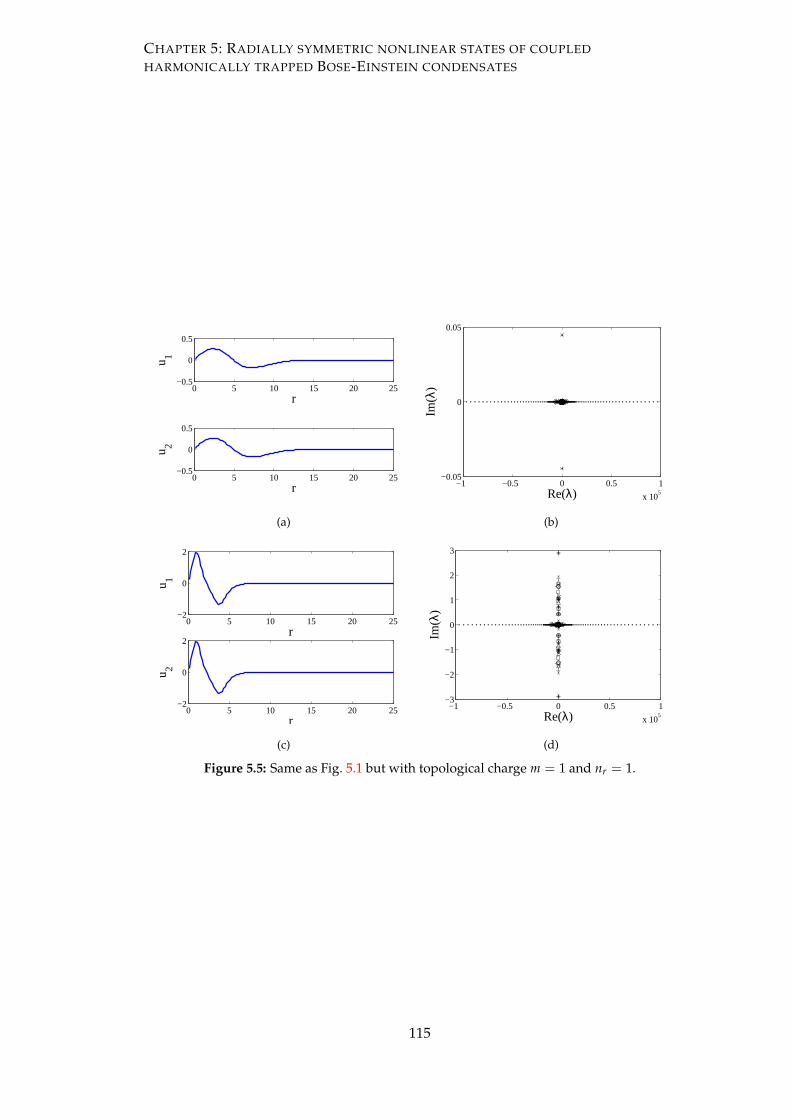
CHAPTER 5: RADIALLY SYMMETRIC NONLINEAR STATES OF COUPLED
HARMONICALLY TRAPPED BOSE-EINSTEIN CONDENSATES
0 5 10 15 20 25−0.5
0
0.5
r
u 1
0 5 10 15 20 25−0.5
0
0.5
r
u 2
(a)
−1 −0.5 0 0.5 1
x 105
−0.05
0
0.05
Re(λ)
Im(λ
)
(b)
0 5 10 15 20 25−2
0
2
r
u 1
0 5 10 15 20 25−2
0
2
r
u 2
(c)
−1 −0.5 0 0.5 1
x 105
−3
−2
−1
0
1
2
3
Re(λ)
Im(λ
)
(d)
Figure 5.5: Same as Fig. 5.1 but with topological charge m = 1 and nr = 1.
115

CHAPTER 5: RADIALLY SYMMETRIC NONLINEAR STATES OF COUPLED
HARMONICALLY TRAPPED BOSE-EINSTEIN CONDENSATES
0 5 10 15 20 25−0.5
0
0.5
r
u 1
0 5 10 15 20 25−0.5
0
0.5
r
u 2
(a)
−1 −0.5 0 0.5 1
x 105
−0.08
−0.06
−0.04
−0.02
0
0.02
0.04
0.06
0.08
Re(λ)
Im(λ
)
(b)
0 5 10 15 20 25−2
0
2
4
r
u 1
0 5 10 15 20 25−2
0
2
4
r
u 2
(c)
−1 −0.5 0 0.5 1
x 105
−5
0
5
Re(λ)
Im(λ
)
(d)
Figure 5.6: Same as Fig. 5.1 but with topological charge m = 1, nr = 2 and ρ0 = 0.8 for
the repulsive case.
116

CHAPTER 5: RADIALLY SYMMETRIC NONLINEAR STATES OF COUPLED
HARMONICALLY TRAPPED BOSE-EINSTEIN CONDENSATES
0 5 10 15 20 250
0.2
0.4
r
u 1
0 5 10 15 20 250
0.2
0.4
r
u 2
(a)
−1 −0.5 0 0.5 1
x 105
−0.05
0
0.05
Re(λ)
Im(λ
)
(b)
0 5 10 15 20 250
0.5
1
1.5
r
u 1
0 5 10 15 20 250
0.5
1
1.5
r
u 2
(c)
−1 −0.5 0 0.5 1
x 105
−3
−2
−1
0
1
2
3
Re(λ)
Im(λ
)
(d)
Figure 5.7: Same as Fig. 5.1 but with topological charge m = 2 and nr = 0.
117

CHAPTER 5: RADIALLY SYMMETRIC NONLINEAR STATES OF COUPLED
HARMONICALLY TRAPPED BOSE-EINSTEIN CONDENSATES
0 5 10 15 20 25−0.5
0
0.5
x
u 1
0 5 10 15 20 25−0.5
0
0.5
x
u 2
(a)
−1 −0.5 0 0.5 1
x 105
−0.1
−0.05
0
0.05
0.1
Re(λ)
Im(λ
)
(b)
0 5 10 15 20 25−2
0
2
r
u 1
0 5 10 15 20 25−2
0
2
r
u 2
(c)
−1 −0.5 0 0.5 1
x 105
−4
−3
−2
−1
0
1
2
3
4
Re(λ)
Im(λ
)
(d)
Figure 5.8: Same as Fig. 5.1 but with topological charge m = 2, nr = 1 and ρ0 = 0.7 for
the repulsive case.
118
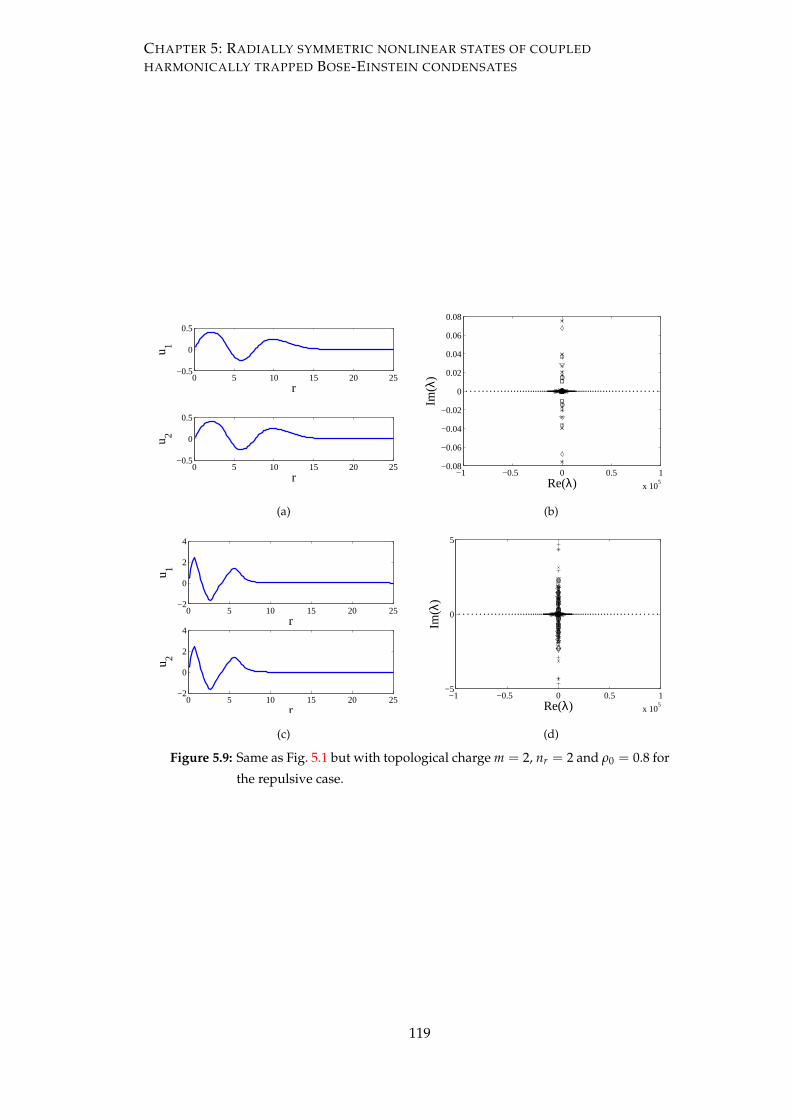
CHAPTER 5: RADIALLY SYMMETRIC NONLINEAR STATES OF COUPLED
HARMONICALLY TRAPPED BOSE-EINSTEIN CONDENSATES
0 5 10 15 20 25−0.5
0
0.5
r
u 1
0 5 10 15 20 25−0.5
0
0.5
r
u 2
(a)
−1 −0.5 0 0.5 1
x 105
−0.08
−0.06
−0.04
−0.02
0
0.02
0.04
0.06
0.08
Re(λ)
Im(λ
)
(b)
0 5 10 15 20 25−2
0
2
4
r
u 1
0 5 10 15 20 25−2
0
2
4
r
u 2
(c)
−1 −0.5 0 0.5 1
x 105
−5
0
5
Re(λ)
Im(λ
)
(d)
Figure 5.9: Same as Fig. 5.1 but with topological charge m = 2, nr = 2 and ρ0 = 0.8 for
the repulsive case.
119

CHAPTER 5: RADIALLY SYMMETRIC NONLINEAR STATES OF COUPLED
HARMONICALLY TRAPPED BOSE-EINSTEIN CONDENSATES
−1 −0.5 0 0.5 1 1.5 20
0.02
0.04
0.06
0.08
0.1
0.12
0.14
µ12
=µ21
Max
(Im
(λ))
q=0q=1q=2q=3q=4
(a)
−1 −0.5 0 0.50
10
20
30
40
50
µ12
=µ21
Max
(Im
(λ))
q=0q=1q=2q=3q=4
(b)
−1 −0.5 0 0.5 1 1.5 20
0.5
1
1.5
2
µ12
=µ21
Max
(Im
(λ))
q=0q=1q=2q=3q=4
(c)
−1 −0.5 0 0.50
20
40
60
80
100
120
µ12
=µ21
Max
(Im
(λ))
q=0q=1q=2q=3q=4
(d)
−1 −0.5 0 0.5 1 1.5 20
0.5
1
1.5
2
2.5
µ12
=µ21
Max
(Im
(λ))
q=0q=1q=2q=3q=4
(e)
−1 −0.5 0 0.50
50
100
150
200
250
µ12
=µ21
Max
(Im
(λ))
q=0q=1q=2q=3q=4
(f)
Figure 5.10: Linear stability curves for non topological charge (m = 0) solutions.
The left and right panels correspond to the repulsive and attractive
intra-atomic interactions, respectively. The upper two panels show the
graphs of maximum imaginary parts as functions of nonlinear coupling
µ12 = µ21 of primary eigenvalues for q = 0, 1, 2, 3, 4 for the ground state
(nr = 0). The middle and the lower panels depict respectively the first
and second excited states. The small magnitude of the unstable eigen-
values in the left panels indicate the slow dynamical development of the
instability. This also reveals that such steady state solutions when per-
turbed slightly, will show deformation or destruction of initial structure
after a relatively long time. On the other hand, the magnitude of the
unstable eigenvalues in the right panels is very high and indicates the
shattering of the structure after a small time.
120

CHAPTER 5: RADIALLY SYMMETRIC NONLINEAR STATES OF COUPLED
HARMONICALLY TRAPPED BOSE-EINSTEIN CONDENSATES
−1 −0.5 0 0.5 1 1.5 20
0.01
0.02
0.03
0.04
0.05
0.06
0.07
0.08
µ12
=µ21
Max
(Im
(λ))
q=0q=1q=2q=3q=4
(a)
−1 −0.5 0 0.50
5
10
15
20
25
30
µ12
=µ21
Max
(Im
(λ))
q=0q=1q=2q=3q=4
(b)
−1 −0.5 0 0.5 1 1.5 2
0.2
0.4
0.6
0.8
1
1.2
1.4
1.6
1.8
µ12
=µ21
Max
(Im
(λ))
q=0q=1q=2q=3q=4
(c)
−1 −0.5 0 0.50
10
20
30
40
50
60
Max
(Im
(λ))
µ12
=µ21
q=0q=1q=2q=3q=4
(d)
−1 −0.5 0 0.5 1 1.5 20
0.5
1
1.5
2
2.5
3
3.5
µ12
=µ21
Max
(Im
(λ))
q=0q=1q=2q=3q=4
(e)
−1 −0.5 0 0.50
10
20
30
40
50
60
70
80
Max
(Im
(λ))
µ12
=µ21
q=0q=1q=2q=3q=4
(f)
Figure 5.11: Same as Fig. 5.10 but for unit topological charge (m = 1) solutions. In
the top left panel, their exist stability regions of nonlinear coupling where
the ground state can be stable for the case of repulsive intra-atomic in-
teraction. The top right panel shows that the ground state for the case of
attractive intra-atomic interaction remains unstable. The remaining pan-
els show that the first and second excited states are unstable in both cases.
121

CHAPTER 5: RADIALLY SYMMETRIC NONLINEAR STATES OF COUPLED
HARMONICALLY TRAPPED BOSE-EINSTEIN CONDENSATES
−1 −0.5 0 0.5 1 1.5 20
0.01
0.02
0.03
0.04
0.05
µ12
=µ21
Max
(Im
(λ))
q=0q=1q=2q=3q=4
(a)
−1 −0.5 0 0.50
5
10
15
20
25
30
35
µ12
=µ21
Max
(Im
(λ))
q=0q=1q=2q=3q=4
(b)
−1 −0.5 0 0.5 1 1.5 20
0.5
1
1.5
2
2.5
µ12
=µ21
Max
(Im
(λ))
q=0q=1q=2q=3q=4
(c)
−1 −0.5 0 0.50
10
20
30
40
50
µ12
=µ21
Max
(Im
(λ))
q=0q=1q=2q=3q=4
(d)
−1 −0.5 0 0.5 1 1.5 20
0.5
1
1.5
2
2.5
µ12
=µ21
Max
(Im
(λ))
q=0q=1q=2q=3q=4
(e)
−1 −0.5 0 0.50
10
20
30
40
50
60
70
µ12
=µ21
Max
(Im
(λ))
q=0q=1q=2q=3q=4
(f)
Figure 5.12: Same as Fig. 5.10 but for doubly charged (m = 2) solutions.
122

CHAPTER 5: RADIALLY SYMMETRIC NONLINEAR STATES OF COUPLED
HARMONICALLY TRAPPED BOSE-EINSTEIN CONDENSATES
Next, we examine the cases of unit (m = 1) and doubly (m = 2) charged solutions.
The top left panels of Fig. 5.11 and Fig. 5.12 show the instability of the ground state in
the defocusing case. However, there exist regions for the values of nonlinear coupling
where stability of these ground states can be possible. In the focusing case, the ground
states are unstable for all values of nonlinear coupling as can be seen in the top right
panels of Fig. 5.11 and Fig. 5.12. Similarly, the first and second excited states are also
unstable in both attractive and repulsive cases (cf. the middle and bottom panels of
Fig. 5.11 and Fig. 5.12).
Let us now investigate the time evolution of each solution in detail. We discuss the
time evolution of each solution when a random perturbation of order 10−4 is added to
the steady state structure at time t = 0. First, we consider the case of m = 0. In the
defocusing case, the ground state for different values of time is shown in Fig. 5.13. The
solution is unstable for the parameter values used due to the q = 0, 1, 2, 3 modes. A
strong inter-atomic repulsion results in the shift of the respective central atomic den-
sities away from the centres in both components, however, in the opposite directions.
The solutions tend to carry all the mass due to the q = 0 mode. Moreover, the solution
is subject to azimuthal modulational instability due to the q = 1, 2, 3 eigenmodes. On
the other hand, the time evolution of the ground state in the focusing case is displayed
in Fig. 5.14. The solution in this case is unstable due to the q = 0, 1 eigenmodes. The
solution in one of the components tends to a thin spike carrying all the mass due to the
q = 0 eigenmode. However, the solution in the other component start rotating due to
the q = 1 eigenmode and results in the reduction of the central atomic density. Also,
the atomic mass is pushed away from the centre due to repulsive interatomic interac-
tion. The central atomic density in this component reduces up to a critical value and
then starts increasing and ultimately tends to a thin spike carrying all the mass at the
centre.
The results obtained for the first excited state with m = 0 in the defocusing case are
demonstrated in Fig. 5.15. The solution is unstable due to the same values of q as for
the ground state. However, the instability rate is comparatively smaller. The central
atomic density peak of the first excited state decays due to the q = 0 mode while the
two humps at t = 200 corroborate the instability due to the q = 2 mode. It is also
evident that the decay of the central atomic density peaks are simultaneously followed
by irregular deposition of atoms on the brim of the basal rings in both components. The
central and the other atomic density peaks localized on the outer brim of the basal ring
become more intense with time. The broadening of the atomic density peaks formed
on the outer rings corresponds to the reduction in the width of central atomic density
123

CHAPTER 5: RADIALLY SYMMETRIC NONLINEAR STATES OF COUPLED
HARMONICALLY TRAPPED BOSE-EINSTEIN CONDENSATES
peaks. The process results in the deformation of outer rings and ultimately the whole
atomic structure breaks up.
On the other hand, for the focusing case in Fig. 5.16, the instability develops as the
eigenmodes corresponding to nonzero values of q induce rotation in the outer rings
in one of the components. The value of cental atomic density in other component in-
creases due to the most unstable mode q = 0 and ultimately results in the appearance
of thin spikes in both components.
Next, we explain the second excited state in the absence of topological charge in Fig.
5.17. Unlike the ground and the first excited states, the solution in the defocusing
case is stable to the q = 0 mode and hence there is no growth or decay seen in the
central atomic density peak. However, the instability appears due to the q = 2 mode.
The instability rate is small like the first excited state. Due to the instability, localized
density peaks appear on the peripheries of first and second rings and grow with time
which results in the destruction of the structure. In Fig. 5.18, for the focusing case, the
decrease in the central atomic density in both components is directly linked with the
increase in the atomic density on the peripheries of the outer rings. Nevertheless, the
solution in both components tend to thin spikes due to the most unstable mode q = 0.
We have discussed the dynamical evolution and stability of non topologically charged
solutions. Now, we take into account the solutions with non-zero topological charge at
the centre of the external magnetic trap. We present the time evolution of the ground
state with unit topological charge m = 1 in Fig. 5.19 and Fig. 5.20 for the defocusing
and focusing cases respectively. The solutions start rotating due to the nonzero value
of m as can be seen at t = 100 and t = 5 respectively in the defocusing and focusing
cases. The vortices urge the atomic mass away from the centre of the trap in both cases.
This act of shoving the atomic mass is a general characteristic in topologically charged
solution.
In Figs. 5.21-5.24, we display the time dynamics of the first and second excited states in
the presence of unit topological charge. In the defocusing case, both states are affected
by very small values of the q = 0, 3 eigenmodes where instability emerges in the rings
of the clouds and results in the deformation of the structures. In the focusing case,
several spikes appear that indicate the instability of the solutions. Finally, we present
the similar results for the stability of ground and excited states in case of topological
charge m = 2 in Figs. 5.25-5.30
124

CHAPTER 5: RADIALLY SYMMETRIC NONLINEAR STATES OF COUPLED
HARMONICALLY TRAPPED BOSE-EINSTEIN CONDENSATES
(a) (b)
(c) (d)
Figure 5.13: Time evolution of the solution shown in the top left panel of Fig. 5.1 in
case of defocusing nonlinearity with m = 0, nr = 0 and µ12 = µ21 = 2.
125

CHAPTER 5: RADIALLY SYMMETRIC NONLINEAR STATES OF COUPLED
HARMONICALLY TRAPPED BOSE-EINSTEIN CONDENSATES
(a) (b)
(c) (d)
Figure 5.14: Time evolution of the solution shown in bottom left panel of Fig. 5.1 in
case of focusing nonlinearity with m = 0, nr = 0 and µ12 = µ21 = 0.2.
126

CHAPTER 5: RADIALLY SYMMETRIC NONLINEAR STATES OF COUPLED
HARMONICALLY TRAPPED BOSE-EINSTEIN CONDENSATES
(a) (b)
(c) (d)
Figure 5.15: Time evolution of the solution shown in the top left panel of Fig. 5.2 in
case of defocusing nonlinearity with m = 0, nr = 1 and µ12 = µ21 = 2.
127

CHAPTER 5: RADIALLY SYMMETRIC NONLINEAR STATES OF COUPLED
HARMONICALLY TRAPPED BOSE-EINSTEIN CONDENSATES
(a) (b)
(c) (d)
Figure 5.16: Time evolution of the solution shown in bottom left panel of Fig. 5.2 in
case of focusing nonlinearity with m = 0, nr = 1 and µ12 = µ21 = 0.2.
128

CHAPTER 5: RADIALLY SYMMETRIC NONLINEAR STATES OF COUPLED
HARMONICALLY TRAPPED BOSE-EINSTEIN CONDENSATES
(a) (b)
(c) (d)
Figure 5.17: Time evolution of the solution shown in the top left panel of Fig. 5.3 in
case of defocusing nonlinearity with m = 0, nr = 2 and µ12 = µ21 = 2.
129

CHAPTER 5: RADIALLY SYMMETRIC NONLINEAR STATES OF COUPLED
HARMONICALLY TRAPPED BOSE-EINSTEIN CONDENSATES
(a) (b)
(c) (d)
Figure 5.18: Time evolution of the solution shown in bottom left panel of Fig. 5.3 in
case of focusing nonlinearity with m = 0, nr = 2 and µ12 = µ21 = 0.2.
130

CHAPTER 5: RADIALLY SYMMETRIC NONLINEAR STATES OF COUPLED
HARMONICALLY TRAPPED BOSE-EINSTEIN CONDENSATES
(a) (b)
(c) (d)
Figure 5.19: Time evolution of the solution shown in the top left panel of Fig. 5.4 in
case of defocusing nonlinearity with m = 1, nr = 0 and µ12 = µ21 = 2.
131

CHAPTER 5: RADIALLY SYMMETRIC NONLINEAR STATES OF COUPLED
HARMONICALLY TRAPPED BOSE-EINSTEIN CONDENSATES
(a) (b)
(c) (d)
Figure 5.20: Time evolution of the solution shown in bottom left panel of Fig. 5.4 in
case of focusing nonlinearity with m = 1, nr = 0 and µ12 = µ21 = 0.2.
132

CHAPTER 5: RADIALLY SYMMETRIC NONLINEAR STATES OF COUPLED
HARMONICALLY TRAPPED BOSE-EINSTEIN CONDENSATES
(a) (b)
(c) (d)
Figure 5.21: Time evolution of the solution shown in the top left panel of Fig. 5.5 in
case of defocusing nonlinearity with m = 1, nr = 1 and µ12 = µ21 = 2.
133

CHAPTER 5: RADIALLY SYMMETRIC NONLINEAR STATES OF COUPLED
HARMONICALLY TRAPPED BOSE-EINSTEIN CONDENSATES
(a) (b)
(c) (d)
Figure 5.22: Time evolution of the solution shown in bottom left panel of Fig. 5.5 in
case of focusing nonlinearity with m = 1, nr = 1 and µ12 = µ21 = 0.2.
134

CHAPTER 5: RADIALLY SYMMETRIC NONLINEAR STATES OF COUPLED
HARMONICALLY TRAPPED BOSE-EINSTEIN CONDENSATES
(a) (b)
(c) (d)
Figure 5.23: Time evolution of the solution shown in the top left panel of Fig. 5.6 in
case of defocusing nonlinearity with m = 1, nr = 2 and µ12 = µ21 = 2.
135

CHAPTER 5: RADIALLY SYMMETRIC NONLINEAR STATES OF COUPLED
HARMONICALLY TRAPPED BOSE-EINSTEIN CONDENSATES
(a) (b)
(c) (d)
Figure 5.24: Time evolution of the solution shown in bottom left panel of Fig. 5.6 in
case of focusing nonlinearity with m = 1, nr = 2 and µ12 = µ21 = 0.2.
136

CHAPTER 5: RADIALLY SYMMETRIC NONLINEAR STATES OF COUPLED
HARMONICALLY TRAPPED BOSE-EINSTEIN CONDENSATES
(a) (b)
(c) (d)
Figure 5.25: Time evolution of the solution shown in the top left panel of Fig. 5.7 in
case of defocusing nonlinearity with m = 2, nr = 0 and µ12 = µ21 = 2.
137

CHAPTER 5: RADIALLY SYMMETRIC NONLINEAR STATES OF COUPLED
HARMONICALLY TRAPPED BOSE-EINSTEIN CONDENSATES
(a) (b)
(c) (d)
Figure 5.26: Time evolution of the solution shown in bottom left panel of Fig. 5.7 in
case of focusing nonlinearity with m = 2, nr = 0 and µ12 = µ21 = 0.2.
138

CHAPTER 5: RADIALLY SYMMETRIC NONLINEAR STATES OF COUPLED
HARMONICALLY TRAPPED BOSE-EINSTEIN CONDENSATES
(a) (b)
(c) (d)
Figure 5.27: Time evolution of the solution shown in the top left panel of Fig. 5.8 in
case of defocusing nonlinearity with m = 2, nr = 1 and µ12 = µ21 = 2.
139

CHAPTER 5: RADIALLY SYMMETRIC NONLINEAR STATES OF COUPLED
HARMONICALLY TRAPPED BOSE-EINSTEIN CONDENSATES
(a) (b)
(c) (d)
Figure 5.28: Time evolution of the solution shown in bottom left panel of Fig. 5.8 in
case of focusing nonlinearity with m = 2, nr = 1 and µ12 = µ21 = 0.2.
140
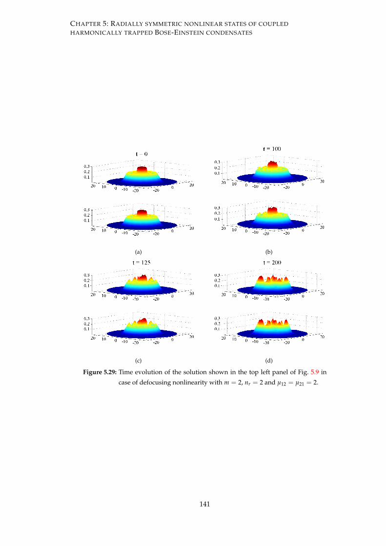
CHAPTER 5: RADIALLY SYMMETRIC NONLINEAR STATES OF COUPLED
HARMONICALLY TRAPPED BOSE-EINSTEIN CONDENSATES
(a) (b)
(c) (d)
Figure 5.29: Time evolution of the solution shown in the top left panel of Fig. 5.9 in
case of defocusing nonlinearity with m = 2, nr = 2 and µ12 = µ21 = 2.
141

CHAPTER 5: RADIALLY SYMMETRIC NONLINEAR STATES OF COUPLED
HARMONICALLY TRAPPED BOSE-EINSTEIN CONDENSATES
(a) (b)
(c) (d)
Figure 5.30: Time evolution of the solution shown in bottom left panel of Fig. 5.9 in
case of focusing nonlinearity with m = 2, nr = 2 and µ12 = µ21 = 0.2.
142

CHAPTER 5: RADIALLY SYMMETRIC NONLINEAR STATES OF COUPLED
HARMONICALLY TRAPPED BOSE-EINSTEIN CONDENSATES
5.4.2 Stability analysis of the linearly coupled system
So far, we considered the case of k = 0. Let us analyze the stability of the solutions
presented above in the case when system of GP Eq. (5.3.1) is linearly coupled, i.e. k = 0
with µ12 = µ21 = 0. The maximum imaginary parts of the primary (q = 0, 1, 2, 3, 4)
eigenvalues for m = 0, 1 and 2, respectively, are displayed in Figs. 5.31-5.33. For each
value of m, the stability curves for the ground and first two excited states are depicted
respectively in left panels for the defocusing case and in the right panels for the focus-
ing case. In Fig. 5.31, the top left and right panels show that the ground states with
m = 0 are unstable in the defocusing and focusing cases. Nonetheless, these states can
be made stable by controlling the value of linear coupling. The stability can be possible
only for the positive values of k in both cases. The first and second excited states with
m = 0 are unstable in focusing and defocusing cases as can be seen in the middle and
lower panels of Fig. 5.31.
The top left panels of Fig. 5.32 and Fig. 5.33 depict that the unit and doubly charged
ground states in the defocusing case are unstable but can be stabilize by adjusting the
value of k. In fact, the ground state with unit topological charge is stable for all positive
values of k where it exists whereas for the ground state with m = 2, there exists zones
of positive values of k where the solution is stable. The other excited states are found
to be unstable.
5.4.3 Stability analysis in the presence of linear and nonlinear coupling
Now, we examine the stability of the solutions of the system of GP Eq. (5.3.1) for the
case when k = 0 and µ12 = µ21 = 0. In this case, we fix the value of nonlinear coupling
and investigate the stability of the solutions with the variation in the value of linear
coupling. The stability curves are shown in Figs. 5.34-5.36. As before, the left panels
show the stability curves for the defocusing case while the right panels depict the fo-
cusing case. One can see in the top left panels of Figs. 5.34-5.36 that the ground states
in the defocusing case in the absence and presence of topological charge can be made
stable by adjusting the values of linear and nonlinear coupling. The top right panels of
Figs. 5.34-5.36 show that in the focusing case, the ground states with or without charge
are unstable. Similarly, the first and second excited states remain unstable in focusing
and defocusing cases as can be seen in the remaining panels of Figs. 5.34-5.36.
143

CHAPTER 5: RADIALLY SYMMETRIC NONLINEAR STATES OF COUPLED
HARMONICALLY TRAPPED BOSE-EINSTEIN CONDENSATES
5.4.4 Stability analysis in case of unequal vorticity in the two components
of BECs
In the above discussion, we considered the cases of equal vorticities in both compo-
nents of BECs, i.e. m1 = m2. Now we will discuss the cases of unequal vorticities, i.e.
m1 = m2 in the defocusing case with k = 0. The stability curves for three different
cases of unequal vorticities with (q = 0, 1, 2, 3, 4) eigenvalues is presented in Fig. 5.37.
First, we consider the case in which one of the components has no topological charge
m1 = 0 while the other component possesses a unit topological charge m2 = 1. The
solution and the corresponding eigenvalues spectra is shown in left and right panels
of Fig. 5.38. The solution is unstable but can be stabilized by controlling the value of
nonlinear coupling as can be seen in the stability curve in Fig. 5.37(a). The time evolu-
tion of the solution is depicted in Fig. 5.38. The solution is unstable due to the q = 0, 1
eigenmodes. One can see that the instability only affects that component which has
a nonzero topological charge. Due to these unstable eigenmodes and the presence of
vorticities, there is fluctuation in the central atomic density peak and on the outer ring
of the component with topological charge. However, the phenomenon looks periodic
and the structure regains itself as can be seen at t = 795. Despite, the fact that the mis-
cibility criteria is satisfied, the component with no vorticities remains stable. The case
of m1 = 0 and m2 = 2 is almost similar as above and is not presented here.
Lastly, we discuss the case of m1 = 1 and m2 = 2. Like the case of m1 = 0 and m2 = 1,
the solution can be made stable by adjusting the value of nonlinear coupling. The so-
lution and the eigenvalues spectra are shown in the upper panels of Fig. 5.39. The
remaining panels of Fig. 5.39 depict the time evolution of the solution. The first excited
state in one of the components appears to be affected due to the q = 0, 1 eigenmodes.
Due the presence of double topological charge, the outer ring and the central atomic
density peak start rotating and results in the deformation of the structure. The other
component carrying unit topological charge also starts rotating. However, the defor-
mation in this component occurs after a relatively longer time as can be seen at time
t = 1500, 2100.
5.5 Conclusion
In this study, we have considered a collection of radially symmetric nonlinear solutions
of a coupled system of GP equations in the presence of a harmonic trap. The numer-
ical linear stability and time dynamics of ground states as well as excited states were
investigated both in the absence and presence of a topological charge. In particular, we
144

CHAPTER 5: RADIALLY SYMMETRIC NONLINEAR STATES OF COUPLED
HARMONICALLY TRAPPED BOSE-EINSTEIN CONDENSATES
−0.4 −0.2 0 0.2 0.4 0.6 0.8 10
0.05
0.1
0.15
0.2
0.25
0.3
0.35
k
Max
(Im
(λ))
q=0q=1q=2q=3q=4
(a)
−1 −0.5 0 0.50
0.2
0.4
0.6
0.8
1
1.2
1.4
k
Max
(Im
(λ))
q=0q=1q=2q=3q=4
(b)
−0.2 0 0.2 0.4 0.6 0.8 10
0.05
0.1
0.15
0.2
0.25
k
Max
(Im
(λ))
q=0q=1q=2q=3q=4
(c)
−1 −0.5 0 0.50
0.5
1
1.5
2
2.5
3
3.5
4
k
Max
(Im
(λ))
q=0q=1q=2q=3q=4
(d)
0 0.2 0.4 0.6 0.8 10
0.05
0.1
0.15
0.2
0.25
k
Max
(Im
(λ))
q=0q=1q=2q=3q=4
(e)
−1 −0.5 0 0.5 10
1
2
3
4
5
k
Max
(Im
(λ))
q=0q=1q=2q=3q=4
(f)
Figure 5.31: Linear stability curves for non topological charge (m = 0) solutions. The
left panels correspond to the defocusing case in which ρ0 = 0.5 while the
right panels correspond to the focusing case in which ρ0 = −0.5. In all
panels µ12 = µ21 = 0. The upper two panels show the graphs of max-
imum imaginary parts as functions of linear coupling of primary eigen-
values for q = 0, 1, 2, 3, 4 for the ground state (nr = 0). The middle and
the lower panels depict respectively the first and second excited states.
The magnitude of the unstable eigenvalues is small in the left panels and
indicates the slow dynamical development of the instability. On the other
hand, the magnitude of the unstable eigenvalues in the right panels is
very high and indicates a rapid deformation of the structure.
145

CHAPTER 5: RADIALLY SYMMETRIC NONLINEAR STATES OF COUPLED
HARMONICALLY TRAPPED BOSE-EINSTEIN CONDENSATES
−0.2 0 0.2 0.4 0.6 0.8 10
0.05
0.1
0.15
0.2
k
Max
(Im
(λ))
q=0q=1q=2q=3q=4
(a)
−1 −0.5 0 0.50
0.5
1
1.5
2
2.5
3
3.5
k
Max
(Im
(λ))
q=0q=1q=2q=3q=4
(b)
0 0.2 0.4 0.6 0.8 10
0.05
0.1
0.15
0.2
0.25
k
Max
(Im
(λ))
q=0q=1q=2q=3q=4
(c)
−1 −0.5 0 0.50
1
2
3
4
5
k
Max
(Im
(λ))
q=0q=1q=2q=3q=4
(d)
0.2 0.4 0.6 0.8 10
0.05
0.1
0.15
0.2
0.25
k
Max
(Im
(λ))
q=0q=1q=2q=3q=4
(e)
−1 −0.5 0 0.5 10
1
2
3
4
5
6
7
8
k
Max
(Im
(λ))
q=0q=1q=2q=3q=4
(f)
Figure 5.32: Same as Fig. 5.31 but for unit topological charge (m = 1) solutions.
146

CHAPTER 5: RADIALLY SYMMETRIC NONLINEAR STATES OF COUPLED
HARMONICALLY TRAPPED BOSE-EINSTEIN CONDENSATES
−0.2 0 0.2 0.4 0.6 0.8 10
0.02
0.04
0.06
0.08
0.1
0.12
0.14
k
Max
(Im
(λ))
q=0q=1q=2q=3q=4
(a)
−1 −0.5 0 0.50
0.5
1
1.5
2
2.5
3
3.5
k
Max
(Im
(λ))
q=0q=1q=2q=3q=4
(b)
0.2 0.4 0.6 0.8 10
0.05
0.1
0.15
0.2
0.25
k
Max
(Im
(λ))
q=0q=1q=2q=3q=4
(c)
−1 −0.5 0 0.5 10
1
2
3
4
5
k
Max
(Im
(λ))
q=0q=1q=2q=3q=4
(d)
0.2 0.4 0.6 0.8 10
0.05
0.1
0.15
0.2
k
Max
(im
(λ))
q=0q=1q=2q=3q=4
(e)
−1 −0.5 0 0.5 10
1
2
3
4
5
6
7
k
Max
(Im
(λ))
q=0q=1q=2q=3q=4
(f)
Figure 5.33: Same as Fig. 5.31 but for doubly charged (m = 2) solutions.
147

CHAPTER 5: RADIALLY SYMMETRIC NONLINEAR STATES OF COUPLED
HARMONICALLY TRAPPED BOSE-EINSTEIN CONDENSATES
−0.4 −0.2 0 0.2 0.4 0.6 0.8 10
0.05
0.1
0.15
0.2
k
Max
(Im
(λ))
q=0q=1q=2q=3q=4
(a)
−1 −0.5 0 0.50
5
10
15
20
k
Max
(Im
(λ))
q=0q=1q=2q=3q=4
(b)
−0.2 0 0.2 0.4 0.6 0.8 10
0.05
0.1
0.15
0.2
0.25
k
Max
(Im
(λ))
q=0q=1q=2q=3q=4
(c)
−1 −0.5 0 0.50
10
20
30
40
50
k
Max
(Im
(λ))
q=0q=1q=2q=3q=4
(d)
0 0.2 0.4 0.6 0.8 10
0.05
0.1
0.15
0.2
0.25
k
Max
(Im
(λ))
q=0q=1q=2q=3q=4
(e)
−1 −0.5 0 0.50
10
20
30
40
50
60
k
Max
(Im
(λ))
q=0q=1q=2q=3q=4
(f)
Figure 5.34: Linear stability curves for non topological charge (m = 0) solutions.
The left panels correspond to the defocusing case in which ρ0 = 0.5,
µ12 = µ21 = 2 while the right panels correspond to the focusing case
in which ρ0 = −0.5, µ12 = µ21 = −0.5. The upper two panels show the
graphs of maximum imaginary parts as functions of linear coupling of
primary eigenvalues for q = 0, 1, 2, 3, 4 for the ground state (nr = 0). The
middle and the lower panels depict respectively the first and second ex-
cited states. The magnitude of the unstable eigenvalues is small in the left
panels and indicates the slow dynamical development of the instability.
On the other hand, the magnitude of the unstable eigenvalues in the right
panels is very high and indicates a rapid deformation of the structure.
148

CHAPTER 5: RADIALLY SYMMETRIC NONLINEAR STATES OF COUPLED
HARMONICALLY TRAPPED BOSE-EINSTEIN CONDENSATES
−0.2 0 0.2 0.4 0.6 0.8 10
0.05
0.1
0.15
0.2
k
Max
(Im
(λ))
q=0q=1q=2q=3q=4
(a)
−1 −0.5 0 0.50
2
4
6
8
10
12
k
Max
(Im
(λ))
q=0q=1q=2q=3q=4
(b)
0 0.2 0.4 0.6 0.8 10
0.05
0.1
0.15
0.2
k
Max
(Im
(λ))
q=0q=1q=2q=3q=4
(c)
−1 −0.5 0 0.50
5
10
15
20
k
Max
(Im
(λ))
q=0q=1q=2q=3q=4
(d)
0.2 0.4 0.6 0.8 10
0.05
0.1
0.15
0.2
k
Max
(Im
(λ))
q=0q=1q=2q=3q=4
(e)
−1 −0.5 0 0.5 10
5
10
15
20
25
30
35
k
Max
(Im
(λ))
q=0q=1q=2q=3q=4
(f)
Figure 5.35: Same as Fig. 5.34 but for unit topological charge (m = 1) solutions.
149

CHAPTER 5: RADIALLY SYMMETRIC NONLINEAR STATES OF COUPLED
HARMONICALLY TRAPPED BOSE-EINSTEIN CONDENSATES
−0.2 0 0.2 0.4 0.6 0.8 10
0.05
0.1
0.15
0.2
k
Max
(Im
(λ))
q=0q=1q=2q=3q=4
(a)
−1 −0.5 0 0.50
2
4
6
8
10
k
Max
(Im
(λ))
q=0q=1q=2q=3q=4
(b)
0.2 0.4 0.6 0.8 10
0.05
0.1
0.15
0.2
k
Max
(Im
(λ))
q=0q=1q=2q=3q=4
(c)
−1 −0.5 0 0.50
2
4
6
8
10
12
14
k
Max
(Im
(λ))
q=0q=1q=2q=3q=4
(d)
0.3 0.4 0.5 0.6 0.7 0.8 0.9 10
0.05
0.1
0.15
0.2
k
Max
(Im
(λ))
q=0q=1q=2q=3q=4
(e)
−1 −0.5 0 0.5 10
5
10
15
20
25
k
Max
(Im
(λ))
q=0q=1q=2q=3q=4
(f)
Figure 5.36: Same as Fig. 5.34 but for doubly charged (m = 2) solutions.
150

CHAPTER 5: RADIALLY SYMMETRIC NONLINEAR STATES OF COUPLED
HARMONICALLY TRAPPED BOSE-EINSTEIN CONDENSATES
0 0.05 0.1 0.15 0.2 0.25 0.3 0.350
0.01
0.02
0.03
0.04
0.05
0.06
0.07
µ12
=µ21
Max
(Im
(λ))
q=0q=1q=2q=3q=4
(a)
0 0.05 0.1 0.15 0.2 0.25 0.30
0.02
0.04
0.06
0.08
0.1
µ12
=µ21
Max
(Im
(λ))
q=0q=1q=2q=3q=4
(b)
0.05 0.1 0.15 0.2 0.25 0.3 0.350
0.01
0.02
0.03
0.04
0.05
0.06
0.07
0.08
µ12
=µ21
Max
(Im
(λ))
q=0q=1q=2q=3q=4
(c)
Figure 5.37: Linear stability curves for the case when (a) one of the components has
zero topological charge m1 = 0 and the other component has unit topo-
logical charge m2 = 1, (b) m1 = 0 and m2 = 2, (c) m1 = 1 and m2 = 2.
151
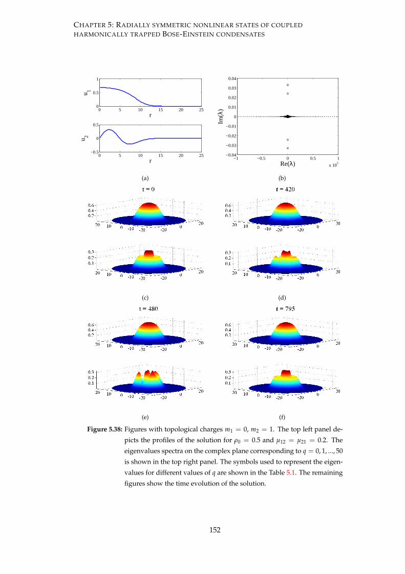
CHAPTER 5: RADIALLY SYMMETRIC NONLINEAR STATES OF COUPLED
HARMONICALLY TRAPPED BOSE-EINSTEIN CONDENSATES
0 5 10 15 20 250
0.5
1
r
u 1
0 5 10 15 20 25−0.5
0
0.5
r
u 2
(a)
−1 −0.5 0 0.5 1
x 105
−0.04
−0.03
−0.02
−0.01
0
0.01
0.02
0.03
0.04
Re(λ)
Im(λ
)
(b)
(c) (d)
(e) (f)
Figure 5.38: Figures with topological charges m1 = 0, m2 = 1. The top left panel de-
picts the profiles of the solution for ρ0 = 0.5 and µ12 = µ21 = 0.2. The
eigenvalues spectra on the complex plane corresponding to q = 0, 1, ..., 50
is shown in the top right panel. The symbols used to represent the eigen-
values for different values of q are shown in the Table 5.1. The remaining
figures show the time evolution of the solution.
152

CHAPTER 5: RADIALLY SYMMETRIC NONLINEAR STATES OF COUPLED
HARMONICALLY TRAPPED BOSE-EINSTEIN CONDENSATES
0 5 10 15 20 250
0.5
1
r
u 1
0 5 10 15 20 25−0.5
0
0.5
r
u 2
(a)
−1 −0.5 0 0.5 1
x 105
−0.04
−0.03
−0.02
−0.01
0
0.01
0.02
0.03
0.04
Re(λ)
Im(λ
)
(b)
(c) (d)
(e) (f)
Figure 5.39: Same as Fig. 5.38 but with topological charges m1 = 1, m2 = 2, µ12 =
µ21 = 0.2 and ρ0 = 0.6.
153

CHAPTER 5: RADIALLY SYMMETRIC NONLINEAR STATES OF COUPLED
HARMONICALLY TRAPPED BOSE-EINSTEIN CONDENSATES
were interested in the linear stability analysis of these states with the variation of linear
or nonlinear coupling. First we considered linear coupling k = 0 and observed that the
ground states with or without vorticities are unstable in both focusing and defocusing
cases. However, it can be possible to stabilize the chargeless and charged ground states
by tuning the nonlinear coupling between the condensates in the defocusing case. The
charged excited states are found to be unstable in both cases. Moreover, the nonlinear
coupling in these cases cannot stabilize the excited states.
Next, we turned the nonlinear coupling off and the linear coupling on, i.e. µ12 = µ21 =
0 and k = 0. All solutions except ground states were found to be unstable. Neverthe-
less, the chargeless ground state in the focusing case can be made stable by adjusting
the value of linear coupling. Also, the chargeless and charged ground states in the de-
focusing case can be made stable by controlling the value of k. We also considered the
case when both linear and nonlinear coupling were nonzero, i.e. µ12 = µ21 = 0 and
k = 0. Again, all solutions were found to be unstable except the ground states of the
defocusing case with or without vorticities which can be stabilize by selecting suitable
values of µ12 = µ21 and k. The ground and higher excited states in the focusing case
were all found to be unstable in the absence and presence of topological charge.
Finally, we studied the stability of the solutions having different values of topological
charge in the defocusing case when linear coupling was off. These solution were found
to be unstable too.
In general, the instability growth rate in all cases of defocusing nonlinearity was found
to be small and shattering of structures in the time evolution appeared after a relatively
long time. On the other hand, in the focusing case, the instability rate was very high
that resulted in the rapid destruction of the structures.
154

CHAPTER 6
Conclusion and Future Work
In this thesis, we have examined the existence and stability of dark solitons and fluxon
analogues (FA) solutions in two effectively one dimensional parallel coupled Bose-
Einstein condensates (BECs) in the presence of an external potential. The interactions
of coupled dark solitons as well as well FA solutions are studied, too. Moreover, the
existence, stability and time dynamics of the ground and higher excited states in the ab-
sence and presence of a topological charge in two-dimensional harmonically trapped
parallel coupled BECs are analyzed. In the following, we summarize our work and
the main results obtained and point out several interesting problems that would be
investigated in the future.
6.1 Summary
We began our discussion in Chapter 1 by providing background information about
solitons and some physical and mathematical aspects of the theory of BECs. These
include the formation of BECs by laser cooling technique and some of its potential
applications. The types of external potential to confine BECs were also presented.
In Chapter 2, a mean-field description of BECs in which Gross-Pitaevskii (GP) equa-
tion that describes their dynamics was derived using a variational approach and the
ground state properties of BECs were presented. The basic nonlinear structures such
as the plane wave solution, the bright solitons and the dark solitons that are ubiqui-
tous in one-dimensional GP equations were considered and their stability analysis was
presented. In the homogeneous case when there was no magnetic trap, the steady
state dark soliton was found to be stable. In the nonhomogeneous case, even though
the presence of magnetic trap affected the profile of the dark soliton, nonetheless the
soliton remained stable.
155

CHAPTER 6: CONCLUSION AND FUTURE WORK
In Chapter 3, we considered two effectively one-dimensional parallel BECs confined
in a double well potential. The condensates were assumed to be linearly coupled by a
weak coupling k. Due to tunnelling and extended spatial dimension along the waveg-
uides, a long Bose-Josephson junction was suggested to be formed by Kaurov and
Kuklov [95, 96]. It was shown that such a system supports atomic Josephson vortex
and can be given by coupled dark-soliton-like solutions. In the thesis, we referred to
these solutions as fluxon analogues (FA). These stable objects can be controlled at high
speed and are used as a basic bit in information processing systems.
We numerically studied the existence and stability of FA solutions and coupled dark
solitons in the absence and presence of a magnetic trap. In carrying out the investi-
gations of the stability of the solitons, the corresponding eigenvalue problems were
solved numerically, and the stability regions for the coupling constant were obtained.
Moreover, numerical integrations of the coupled system of GP equations were per-
formed to verify the results of the stability of solitons.
We began with the case when there was no trap and obtained the coupled dark solitons
numerically. The dark solitons were found to be unstable below a critical coupling kcs
but became stable for k ≥ kcs. It was observed that the dark solitons emit radiation
when they become unstable. In the instability region of coupled dark solitons, an FA
solution was obtained. The FA solution was found to exist below a critical value kce. At
k = kce, it transformed into a coupled dark soliton. Both FA and coupled dark solitons
coincided at k = kce in a pitchfork bifurcation. FA solution was found to be stable in its
domain of existence.
We extended the work in [95, 96] and investigated the existence, stability and time
dynamics of FA solutions and coupled dark solitons in the presence of a harmonic
trap. It was noted that the external potential did not affect the domain of existence
of FA solution. However, the presence of the trap destabilized the FA solution. Due
to the instability, FA solution started oscillating about the minimum of the trap non-
sinusoidally. It was shown that the FA solution can be stabilized by adjusting the linear
coupling between the condensates. The existence and stability of coupled dark solitons
could not be influenced by the presence of trap.
Next, a travelling FA solution was obtained numerically and deformation in its profile
was seen due to non-zero value of velocity v. We then found the domain of existence
for k corresponding to different values of velocity for FA solution. It was noted that
the critical value kce at which solution changes into a coupled dark soliton reduced
with v. Nevertheless, the travelling FA solution remained stable in its entire domain of
existence like static FA solution. The travelling dark solitons were found to be unstable
156
CHAPTER 6: CONCLUSION AND FUTURE WORK
for k < kce and were stable for k ≥ kce. We also derived a relationship between the
velocity v and critical coupling kce analytically. The relation was compared with the
numerical results showing excellent agreement.
To study the dynamical behavior of FA solutions analytically, a variational approach
was employed to approximate the solutions. The Lagrangian formalism was separated
into two cases, i.e. when the coupling constant k was close to the critical coupling kce at
which the FA solutions were close to coupled dark solitons and when it was close to the
uncoupled limit k ≈ 0. In the former case, the oscillation frequency of dark solitons in a
harmonic trap which was first presented by Busch and Anglin in [125] was recovered.
In the latter case, the solution was approximated using an ansatz similar to Gaussian
ansatz and a good approximation is obtained. The theoretical approximations were
used to explain the results obtained numerically.
In Chapter 4, we attempted to investigate the existence, stability and dynamics of mul-
tiple FA solutions and coupled dark solitons in linearly coupled BECs. In particular,
we examined the prototypical cases of two and three FA solutions and dark solitons.
First, we considered the uncoupled case, i.e. k = 0 and analyzed the homogeneous
weakly interacting case of a symmetric collision of two dark solitons. A formula for
the effective repulsive potential in this case was derived and then generalized it for
the cases of asymmetric collisions and an arbitrary number of dark solitons. Next, we
considered the coupled nonhomogeneous system of GP equations and determined the
in-phase and out-of-phase oscillation frequencies of two and three FA solutions in the
limit of k ≈ kce. This has been done by incorporating the effective repulsive potential
with the external harmonic potential using a variational approach and qualitatively
good approximations were obtained.
The interactions of dark solitons in the uncoupled case were first investigated in [97].
We then studied the interactions of multiple coupled dark solitons and FA solutions
in the absence and presence of a harmonic trap. First, we took into consideration the
homogeneous case. The symmetric and asymmetric collisions of multiple dark solitons
were analyzed in Section 4.4.2. In symmetric cases, it was observed that two slow
moving dark solitons repelled each other at the point of their closest proximity while
fast moving solitons transmitted through each other. In cases of asymmetric collisions,
the moving solitons transferred all their energy to static solitons and became static after
collision. The interaction scenarios of the coupled dark solitons were found almost
similar to interactions in the uncoupled cases. The only difference was the emergence
of radiation which was not seen in the uncoupled case.
Next, we studied the interactions of multiple FA solutions. In case of symmetric col-
157

CHAPTER 6: CONCLUSION AND FUTURE WORK
lisions, two types of possible interactions of FA solutions were introduced. From the
symmetry of the imaginary parts, the first possibility was referred to as the odd sym-
metric interaction or (+−)-configuration and the second possibility as even symmetric
interaction or (++)-configuration. It was noticed that in case of odd symmetric col-
lisions, two slow moving FA solutions showed attraction towards each other at the
interaction point and phase shift was induced. The fast moving FA solutions passed
through each other due to their high velocities without changing their phase. On the
other hand, in case of even symmetric collisions, two slow moving FA solutions formed
a breather similar to that reported in [133] in a parametrically driven Schrödinger equa-
tion while the fast moving FA solutions collide and become unidentifiable.
We also examined the existence, stability and time dynamics of stationary multiple FA
solutions and coupled dark solitons in the presence of a magnetic trap. In particular,
we studied that how the domains of existence and stability of these multiple states
varies with the trapping strength. Our calculations showed that the (+−) and (+−+)-
configurations of FA solutions were unstable in their domains of existence. For the
(++) and (+++)- configurations of FA solutions, there exist regions of stability where
these configurations were found to be stable.
In Chapter 5, we considered two effectively two-dimensional parallel coupled BECs
confined in a double well potential. The system was modelled by two GP equations
coupled by linear and nonlinear terms. We used the polar coordinates and converted
the GP equations to polar form. A large set of radially symmetric nonlinear solutions
of the coupled system of GP equations in the presence of a harmonic trap was taken
into account. The existence, linear stability and time dynamics of nontopological and
topologically charged ground and higher excited states were analyzed numerically.
In particular, we were concerned about the stability of radially symmetric states with
the variation in linear or nonlinear coupling. First, we considered the case when the
condensates were nonlinearly coupled and the linear coupling was off. It was found
that the chargeless and charged ground state solutions in the focusing and defocusing
cases are unstable. Nevertheless, in the defocusing case, stabilization of the charge-
less and charged ground state solutions was possible by manipulating the nonlinear
coupling between the condensates. On the contrary, the ground states with or with-
out a charge in the focusing case remained unstable. Unlike the defocusing case, these
states could not be stabilized through nonlinear coupling. Similarly, the charged ex-
cited states were shown to be unstable in focusing and defocusing cases.
Then we dealt with the situations when the nonlinear coupling was inoperative and the
condensates were only linearly coupled. The ground and all higher excited states were
158
CHAPTER 6: CONCLUSION AND FUTURE WORK
found to be unstable in both focusing and defocusing cases. However, it was possible
to stabilize the chargeless ground states in focusing and defocusing cases by controlling
the linear coupling. The same was true for the charged ground states in the defocusing
case. We also considered the stability of nonlinear states in the presence of linear and
nonlinear coupling. It was shown that only the chargeless and charged ground states
in the defocusing case can be made stable with an appropriate choice of values of linear
and nonlinear couplings. Finally, we examined the stability of the nonlinear states in
the defocusing case when the condensates were nonlinearly coupled and had different
values of topological charge in the two components. All solutions were found to be
unstable.
6.2 Future work
We identify several problems in this section that could be intriguing for future work.
Some of these problems originate from the development of the ideas of the present
work, while others emanate from the questions raised during this study that call for
analysis.
One of the possible problems is to reconsider the work of Chapters 3 and 4 in a finite
spatial dimension by incorporating the periodic boundary conditions. The situation
corresponds the case of confining BECs in two concentric rings in the presence of ex-
ternal harmonic trap which was considered in [109]. The transverse excitations in each
ring were assumed to be squeezed and the condensates were supposed to be linearly
coupled in absolutely one dimension and hence can be modelled by the coupled system
of GP Eq. (3.1.1). The effects of the trapping strength on the existence and stability of
the dark solitons and FA solutions could be investigated. Furthermore, the interactions
of coupled dark solitons and FA solutions in the absence and presence of a harmonic
potential could be examined.
Another interesting problem that could be pursued in future is to study the dynamics
of linearly coupled one-dimensional BECs with repulsive interatomic interaction in the
presence of magnetic trap by dragging an obstacle through the condensates. The ob-
stacle can be created by using a blue-detuned laser beam that acts as a potential and
can be given by Gaussian function Ae−x2/σ2, where A and σ represent respectively the
strength and width of the laser obstacle [145]. The analysis of the generation of grey
solitons by dragging an obstacle through a quasi one-dimensional trapped BEC was
presented in [146]. It was shown that the generation of grey solitons depends on the
velocity and shape of the obstacle. In a coupled system of BECs, FA solutions and dark
159

CHAPTER 6: CONCLUSION AND FUTURE WORK
solitons can be expected to exist in a specific domain for dragging velocity and may
show bifurcation.
Next, it could be fascinating to extend the study of Chapter 5 for coupled Gross-Pitaevskii
system to the full three dimensional problem, similarly as before by considering the ra-
dially symmetric states and investigating the linear stability as well as time dynamics.
However, the numerical computations in this case will be rich and comprehensive.
An interesting model that has important applications in nonlinear optics and atomic
physics is the discrete nonlinear Schrödinger equation. This equation arises in the
description of a BEC confined in deep periodic optical lattices. These lattices split
the condensate into an array of droplets. As our study in this thesis was focused on
the coupled nonlinear GP equations, parallel to this study, one can consider the one-
dimensional linearly coupled system of discrete nonlinear Schrödinger equations given
by
iΨjn = −C
(Ψj
n+1 − 2Ψjn + Ψj
n−1
)+ µ|Ψj
n|2Ψjn − ρ0Ψj
n − kΨ3−jn ,
where j = 1, 2 and dot represents the derivative with respect to time t. Here, the
spatial variable is discrete and the evolution variable is continuous. The parameter
C denotes the coupling between the adjacent optical lattice potentials. µ and ρ0 are
respectively the nonlinearity coefficient and chemical potential. k is the linear coupling
between the two condensates. The above coupled system admits different types of
configurations. In particular, we could consider discrete coupled dark solitons and FA
solutions. Once an exact solution of a specific configuration with C = 0 is constructed,
it could be numerically continued to obtain the solution for non-zero values of C. Then
the existence, stability and dynamics of these discrete structures could be investigated.
160

References
[1] J. S. Russell. Report on waves. Fourteenth meeting of the British Association for the
Advancement of Science, London, 1845.
[2] A. Scott. Nonlinear Science: Emergence and Dynamics of Coherent Structures. Oxford
University Press, New York, USA, 2003.
[3] V. E. Zakharov and A. B. Shabat. Exact theory of two-dimensional self-focusing
and one-dimensional self-modulation of waves in nonlinear media. Sov. Phys.
JETP, 34:62–69, 1972.
[4] J. R. Taylor. Optical solitons: Theory and Experiment. Cambridge University Press,
New York, USA, 1992.
[5] I. Calder, A. Ovassapian, and N. Calder. John Logie Baird–fibreoptic pioneer. J.
R. Soc. Med., 93(8):438–439, 2000.
[6] G. I. A. Stegeman, D. N. Christodoulides, and M. Segev. Optical spatial solitons:
Historical perspectives. IEEE J. Sel. Topics Quantum Electron, 6(6):1419–1427, 2000.
[7] Y. S. Kivshar and X. Yang. Perturbation-induced dynamics of dark solitons. Phys.
Rev. E, 49(2):1657, 1994.
[8] C. S. Gardner, J. M. Greene, M. D. Kruskal, and R. M. Miura. Method for solving
the Korteweg-deVries equation. Phys. Rev. Lett., 19(19):1095–1097, 1967.
[9] G. P. Agrawal. Applications of nonlinear fiber optics. Academic press, USA, 2008.
[10] C. Sulem and P. L. Sulem. The nonlinear Schrödinger equation: self-focusing and wave
collapse. Springer, New York, USA, 1999.
[11] K. B. Dysthe. Note on a modification to the nonlinear Schrödinger equation for
application to deep water waves. Proc. Roy. Soc. London Ser. A. Math. Phys. Sci.,
369(1736):105–114, 1979.
161

REFERENCES
[12] D. H. Peregrine. Water waves, nonlinear Schrödinger equations and their solu-
tions. J. Austral. Math. Soc. Ser. B, 25(01):16–43, 1983.
[13] K. Trulsen and K. B. Dysthe. A modified nonlinear Schrödinger equation for
broader bandwidth gravity waves on deep water. Wave motion, 24(3):281–289,
1996.
[14] T. Taniuti and H. Washimi. Self-trapping and instability of hydromagnetic waves
along the magnetic field in a cold plasma. Phys. Rev. Lett., 21(4):209–212, 1968.
[15] E. P. Gross. Hydrodynamics of a superfluid condensate. J. Math. Phys., 4:195,
1963.
[16] L. P. Pitaevskii. Vortex lines in an imperfect Bose gas. Sov. Phys. JETP, 13(2):
451–454, 1961.
[17] I. S. Aranson and L. Kramer. The world of the complex Ginzburg-Landau equa-
tion. Rev. Mod. Phys., 74(1):99–143, 2002.
[18] M. C. Cross and P. C. Hohenberg. Pattern formation outside of equilibrium. Rev.
Mod. Phys., 65(3):851–1112, 1993.
[19] A. Hasegawa and F. Tappert. Transmission of stationary nonlinear optical pulses
in dispersive dielectric fibers. I. anomalous dispersion. Appl. Phys. Lett., 23(3):
142–144, 1973.
[20] L. F. Mollenauer, R. H. Stolen, and J. P. Gordon. Experimental observation of
picosecond pulse narrowing and solitons in optical fibers. Phys. Rev. Lett., 45(13):
1095–1098, 1980.
[21] L. F. Mollenauer, M. J. Neubelt, S. G. Evangelides, J. P. Gordon, J. R. Simpson, and
L. G. Cohen. Experimental study of soliton transmission over more than 10,000
km in dispersion-shifted fiber. Opt. Lett., 15(21):1203–1205, 1990.
[22] A. Afroozeh, I. S. Amiri, M. Kouhnavard, M. A. Jalil, J. Ali, and P. P. Yupapin.
Optical dark and bright soliton generation and amplification. AIP Conf. Proc.,
1341:259–263, 2010.
[23] P. A. Ruprecht, M. J. Holland, K. Burnett, and M. Edwards. Time-dependent so-
lution of the nonlinear Schrödinger equation for Bose-condensed trapped neutral
atoms. Phys. Rev. A, 51(6):4704–4711, 1995.
[24] K. E. Strecker, G. B. Partridge, A. G. Truscott, and R. G. Hulet. Formation and
propagation of matter-wave soliton trains. Nature, 417(6885):150–153, 2002.
162

REFERENCES
[25] L. Khaykovich, F. Schreck, G. Ferrari, T. Bourdel, J. Cubizolles, L. D. Carr,
Y. Castin, and C. Salomon. Formation of a matter-wave bright soliton. Science,
296(5571):1290–1293, 2002.
[26] A. Hasegawa and F. Tappert. Transmission of stationary nonlinear optical pulses
in dispersive dielectric fibers. II. normal dispersion. Appl. Phys. Lett., 23(4):171–
172, 1973.
[27] A. M. Weiner, J. P. Heritage, R. J. Hawkins, R. N. Thurston, E. M. Kirschner, D. E.
Leaird, and W. J. Tomlinson. Experimental observation of the fundamental dark
soliton in optical fibers. Phys. Rev. Lett., 61(21):2445–2448, 1988.
[28] D. Krökel, N. J. Halas, G. Giuliani, and D. Grischkowsky. Dark-pulse propagation
in optical fibers. Phys. Rev. Lett., 60(1):29–32, 1988.
[29] M. Lisak, D. Anderson, and B. A. Malomed. Dissipative damping of dark solitons
in optical fibers. Opt. Lett., 16(24):1936–1937, 1991.
[30] Y. S. Kivshar and V. V. Afanasjev. Dark optical solitons with reverse-sign ampli-
tude. Phys. Rev. A, 44(3):R1446–R1449, 1991.
[31] Y. Chen and J. Atai. Absorption and amplification of dark solitons. Opt. Lett., 16
(24):1933–1935, 1991.
[32] B. Luther-Davies and X. Yang. Steerable optical waveguides formed in self-
defocusing media by using dark spatial solitons. Opt. Lett, 17(24):1755–1757,
1992.
[33] P. Emplit, M. Haelterman, and J. P. Hamaide. Picosecond dark soliton over a
1-km fiber at 850 nm. Opt. Lett., 18(13):1047–1049, 1993.
[34] S. Burger, K. Bongs, S. Dettmer, W. Ertmer, K. Sengstock, A. Sanpera, G. V.
Shlyapnikov, and M. Lewenstein. Dark solitons in Bose-Einstein condensates.
Phys. Rev. Lett., 83(25):5198–5201, 1999.
[35] Y. S. Kivshar and B. Luther-Davies. Dark optical solitons: physics and applica-
tions. Phys. Rep., 298(2):81–197, 1998.
[36] M. Chen, M. A. Tsankov, J. M. Nash, and C. E. Patton. Microwave magnetic-
envelope dark solitons in yttrium iron garnet thin films. Phys. Rev. Lett., 70(11):
1707–1710, 1993.
[37] B. Denardo, W. Wright, S. Putterman, and A. Larraza. Observation of a kink
soliton on the surface of a liquid. Phys. Rev. Lett., 64(13):1518–1521, 1990.
163

REFERENCES
[38] C. Elphick and E. Meron. Localized structures in surface waves. Phys. Rev. A, 40
(6):3226–3229, 1989.
[39] B. Denardo, B. Galvin, A. Greenfield, A. Larraza, S. Putterman, and W. Wright.
Observations of localized structures in nonlinear lattices: Domain walls and
kinks. Phys. Rev. Lett., 68(11):1730–1733, 1992.
[40] B. A. Malomed. Soliton management in periodic systems. Springer New York, 2006.
[41] M. H. Anderson, J. R. Ensher, M. R. Matthews, C. E. Wieman, and E. A. Cornell.
Observation of Bose-Einstein condensation in a dilute atomic vapor. science, 269
(5221):198–201, 1995.
[42] K. B. Davis, M. O. Mewes, M. R. Andrews, N. J. van Druten, D. S. Durfee, D. M.
Kurn, and W. Ketterle. Bose-Einstein condensation in a gas of sodium atoms.
Phys. Rev. Lett., 75(22):3969–3973, 1995.
[43] W. Pauli. Z. Physik, 31:765, 1925.
[44] Cohen-Tannoudji, N. Claude, and W. D. Phillips. New mechanisms for laser
cooling. Phys. Today, 43(10):33, 1990.
[45] T. Dauxois and M. Peyrard. Physics of solitons. Cambridge University Press, 2006.
[46] C. J. Pethick and H. Smith. Bose-Einstein condensation in dilute gases. Cambridge
University Press, 2002.
[47] L. V. Hau, S. E. Harris, Z. Dutton, and H. C. Behroozi. Light speed reduction to
17 metres per second in an ultracold atomic gas. Nature, 397(6720):594–598, 1999.
[48] S. N. Ginsberg, S. R. Garner, and L. V. Hau. Coherent control of optical informa-
tion with matter wave dynamics. Nature, 445(7128):623–626, 2007.
[49] E. A. Cornell and C. E. Wieman. Nobel lecture: Bose-Einstein condensation in a
dilute gas, the first 70 years and some recent experiments. Rev. Mod. Phys., 74(3):
875–893, 2002.
[50] D. S. Petrov, G. V. Shlyapnikov, and J. T. M. Walraven. Regimes of quantum
degeneracy in trapped 1D gases. Phys. Rev. Lett., 85(18):3745–3749, 2000.
[51] D. S. Petrov, G. V. Shlyapnikov, and J. T. M. Walraven. Phase-fluctuating 3D Bose-
Einstein condensates in elongated traps. Phys. Rev. Lett., 87(5):050404, 2001.
[52] J. O. Andersen, U. Al Khawaja, and H. T. C. Stoof. Phase fluctuations in atomic
Bose gases. Phys. Rev. Lett., 88(7):070407, 2002.
164

REFERENCES
[53] A. Görlitz, J. M. Vogels, A. E. Leanhardt, C. Raman, T. L. Gustavson, J. R. Abo-
Shaeer, A. P. Chikkatur, S. Gupta, S. Inouye, T. Rosenband, and W. Ketterle. Re-
alization of Bose-Einstein condensates in lower dimensions. Phys. Rev. Lett., 87
(13):130402, 2001.
[54] M. Greiner, I. Bloch, O. Mandel, W. T. Hänsch, and T. Esslinger. Exploring phase
coherence in a 2D lattice of Bose-Einstein condensates. Phys. Rev. Lett., 87(16):
160405, 2001.
[55] J. H. Denschlag, J. E. Simsarian, H. Häffner, C. McKenzie, A. Browaeys, D. Cho,
K. Helmerson, S. L. Rolston, and W. D. Phillips. A Bose-Einstein condensate in
an optical lattice. J. Phys. B: At., Mol. Opt. Phys., 35(14):3095, 2002.
[56] D. M. Stamper-Kurn, M. R. Andrews, A. P. Chikkatur, S. Inouye, H.-J. Miesner,
J. Stenger, and W. Ketterle. Optical confinement of a Bose-Einstein condensate.
Phys. Rev. Lett., 80(10):2027–2030, 1998.
[57] M. D. Barrett, J. A. Sauer, and M. S. Chapman. All-optical formation of an atomic
Bose-Einstein condensate. Phys. Rev. Lett., 87(1):010404, 2001.
[58] M. Albiez, R. Gati, J. Fölling, S. Hunsmann, M. Cristiani, and M. K. Oberthaler.
Direct observation of tunnelling and nonlinear self-trapping in a single Bosonic
Josephson junction. Phys. Rev. Lett., 95(1):010402, 2005.
[59] B. P. Anderson and M. A. Kasevich. Macroscopic quantum interference from
atomic tunnel arrays. Science, 282(5394):1686–1689, 1998.
[60] M. R. Andrews, C. G. Townsend, H.-J. Miesner, D. S. Durfee, D. M. Kurn, and
W. Ketterle. Observation of interference between two Bose condensates. Science,
275(5300):637–641, 1997.
[61] W. Hänsel, P. Hommelhoff, T. W. Hänsch, and J. Reichel. Bose-Einstein conden-
sation on a microelectronic chip. Nature, 413(6855):498–501, 2001.
[62] H. Ott, J. Fortagh, G. Schlotterbeck, A. Grossmann, and C. Zimmermann. Bose-
Einstein condensation in a surface microtrap. Phys. Rev. Lett., 87(23):230401, 2001.
[63] D. J. Kaup and T. K. Vogel. Quantitative measurement of variational approxima-
tions. Phys. Lett. A, 362(4):289–297, 2007.
[64] B. A. Malomed. Variational methods in nonlinear fiber optics and related fields.
Prog. Optics, 43:71–193, 2002.
165

REFERENCES
[65] A. J. Leggett. Bose-Einstein condensation in the alkali gases: Some fundamental
concepts. Rev. Mod. Phys., 73(2):307–356, 2001.
[66] G. F. Gribakin and V. V. Flambaum. Calculation of the scattering length in atomic
collisions using the semiclassical approximation. Phys. Rev. A, 48(1):546–553,
1993.
[67] C. A. Sackett, J. M. Gerton, M. Welling, and R. G. Hulet. Measurements of col-
lective collapse in a Bose-Einstein condensate with attractive interactions. Phys.
Rev. Lett., 82(5):876–879, 1999.
[68] E. A. Donley, N. R. Claussen, S. L. Cornish, J. L. Roberts, E. A. Cornell, and C. E.
Wieman. Dynamics of collapsing and exploding Bose-Einstein condensates. na-
ture, 2001.
[69] F. Dalfovo, S. Giorgini, L. P. Pitaevskii, and S. Stringari. Theory of Bose-Einstein
condensation in trapped gases. Rev. Mod. Phys., 71(3):463–512, 1999.
[70] R. Carretero-González, D. J. Frantzeskakis, and P. G. Kevrekidis. Nonlinear
waves in Bose-Einstein condensates: physical relevance and mathematical tech-
niques. Nonlinearity, 21(7):R139, 2008.
[71] V. E. Zakharov and A. B. Shabat. Interaction between solitons in a stable medium.
Sov. Phys. JETP, 37:823, 1973.
[72] Y. S. Kivshar and W. Królikowski. Lagrangian approach for dark solitons. Opt.
Commun., 114(3):353–362, 1995.
[73] L. D. Menza and C. Gallo. The black solitons of one-dimensional NLS equations.
Nonlinearity, 20(2):461, 2007.
[74] D. E. Pelinovsky and P. G. Kevrekidis. Dark solitons in external potentials.
Angew. Math. Phys., 59(4):559–599, 2008.
[75] C. C. Bradley, C. A. Sackett, and R. G. Hulet. Bose-Einstein condensation of
lithium: Observation of limited condensate number. Phys. Rev. Lett., 78(6):985–
989, 1997.
[76] C. J. Myatt, E. A. Burt, R. W. Ghrist, E. A. Cornell, and C. E. Wieman. Production
of two overlapping Bose-Einstein condensates by sympathetic cooling. Phys. Rev.
Lett., 78(4):586–589, 1997.
166

REFERENCES
[77] J. Stenger, S. Inouye, D. M. Stamper-Kurn, H. J. Miesner, A. P. Chikkatur, and
W. Ketterle. Spin domains in ground state Bose-Einstein condensates. nature,
1998.
[78] G. Roati R. J. Brecha A. Simoni M. Inguscio G. Modugno, G. Ferrari. Bose-Einstein
condensation of potassium atoms by sympathetic cooling. Science, 294(5545):
1320, 2001.
[79] M. Mudrich, S. Kraft, K. Singer, R. Grimm, A. Mosk, and M. Weidemüller. Sym-
pathetic cooling with two atomic species in an optical trap. Phys. Rev. Lett., 88
(25):253001, 2002.
[80] D. Ananikian and T. Bergeman. Gross-Pitaevskii equation for Bose particles in a
double-well potential: Two-mode models and beyond. Phys. Rev. A, 73(1):013604,
2006.
[81] F. Dalfovo and S. Stringari. Bosons in anisotropic traps: Ground state and vor-
tices. Phys. Rev. A, 53(4):2477–2485, 1996.
[82] K.-P. Marzlin, W. Zhang, and E. M. Wright. Vortex coupler for atomic Bose-
Einstein condensates. Phys. Rev. Lett., 79(24):4728–4731, 1997.
[83] B. M. Caradoc-Davies, R. J. Ballagh, and K. Burnett. Coherent dynamics of vortex
formation in trapped Bose-Einstein condensates. Phys. Rev. Lett., 83(5):895–898,
1999.
[84] H. Susanto, P. G. Kevrekidis, R. Carretero-González, B. A. Malomed, D. J.
Frantzeskakis, and A. R. Bishop. Cerenkov-like radiation in a binary superfluid
flow past an obstacle. Phys. Rev. A, 75(5):055601, 2007.
[85] M. R. Matthews, B. P. Anderson, P. C. Haljan, D. S. Hall, C. E. Wieman, and E. A.
Cornell. Vortices in a Bose-Einstein condensate. Phys. Rev. Lett., 83(13):2498–2501,
1999.
[86] F. Chevy, K. W. Madison, and J. Dalibard. Measurement of the angular momen-
tum of a rotating Bose-Einstein condensate. Phys. Rev. Lett., 85(11):2223–2227,
2000.
[87] K. W. Madison, F. Chevy, W. Wohlleben, and J. Dalibard. Vortex formation in a
stirred Bose-Einstein condensate. Phys. Rev. Lett., 84(5):806–809, 2000.
[88] E. Hodby, G. Hechenblaikner, S. A. Hopkins, O. M. Maragò, and C. J. Foot. Vortex
nucleation in Bose-Einstein condensates in an oblate, purely magnetic potential.
Phys. Rev. Lett., 88(1):010405, 2001.
167

REFERENCES
[89] B. Jackson, J. F. McCann, and C. S. Adams. Vortex formation in dilute inhomoge-
neous Bose-Einstein condensates. Phys. Rev. Lett., 80(18):3903–3906, 1998.
[90] T. Winiecki, J. F. McCann, and C. S. Adams. Pressure drag in linear and nonlinear
quantum fluids. Phys. Rev. Lett., 82(26):5186–5189, 1999.
[91] D. R. Scherer, C. N. Weiler, T. W. Neely, and B. P. Anderson. Vortex formation by
merging of multiple trapped Bose-Einstein condensates. Phys. Rev. Lett., 98(11):
110402, 2007.
[92] R. Carretero-González, B. P. Anderson, P. G. Kevrekidis, D. J. Frantzeskakis, and
C. N. Weiler. Dynamics of vortex formation in merging Bose-Einstein condensate
fragments. Phys. Rev. A, 77(3):033625, 2008.
[93] K. W. Madison, F. Chevy, V. Bretin, and J. Dalibard. Stationary states of a rotating
Bose-Einstein condensate: Routes to vortex nucleation. Phys. Rev. Lett., 86(20):
4443–4446, 2001.
[94] B. Deconinck, P. G. Kevrekidis, H. E. Nistazakis, and D. J. Frantzeskakis. Linearly
coupled Bose-Einstein condensates: From Rabi oscillations and quasiperiodic so-
lutions to oscillating domain walls and spiral waves. Phys. Rev. A, 70(6):063605,
2004.
[95] V. M. Kaurov and A. B. Kuklov. Josephson vortex between two atomic Bose-
Einstein condensates. Phys. Rev. A, 71(1):011601, 2005.
[96] V. M. Kaurov and A. B. Kuklov. Atomic Josephson vortices. Phys. Rev. A, 73(1):
013627, 2006.
[97] G. Theocharis, A. Weller, J. P. Ronzheimer, C. Gross, M. K. Oberthaler, P. G.
Kevrekidis, and D. J. Frantzeskakis. Multiple atomic dark solitons in cigar-
shaped Bose-Einstein condensates. Phys. Rev. A, 81(6):063604, 2010.
[98] G. Herring, L. D. Carr, R. Carretero-González, P. G. Kevrekidis, and D. J.
Frantzeskakis. Radially symmetric nonlinear states of harmonically trapped
Bose-Einstein condensates. Phys. Rev. A, 77(2):023625, 2008.
[99] B. D. Josephson. Possible new effects in superconductive tunnelling. Phys. Lett.,
1:251–253, 1962.
[100] A. Smerzi, S. Fantoni, S. Giovanazzi, and S. R. Shenoy. Quantum coherent atomic
tunnelling between two trapped Bose-Einstein condensates. Phys. Rev. Lett., 79
(25):4950–4953, 1997.
168
REFERENCES
[101] S. Raghavan, A. Smerzi, S. Fantoni, and S. R. Shenoy. Coherent oscillations be-
tween two weakly coupled Bose-Einstein condensates: Josephson effects, π os-
cillations, and macroscopic quantum self-trapping. Phys. Rev. A, 59(1):620–633,
1999.
[102] S. Giovanazzi, A. Smerzi, and S. Fantoni. Josephson effects in dilute Bose-
Einstein condensates. Phys. Rev. Lett., 84(20):4521–4524, 2000.
[103] S. Levy, E. Lahoud, I. Shomroni, and J. Steinhauer. The a.c. and d.c. Josephson
effects in a Bose-Einstein condensate. Nature, 449(7162):579–583, 2007.
[104] F. S. Cataliotti, S. Burger, C. Fort, P. Maddaloni, F. Minardi, A. Trombettoni,
A. Smerzi, and M. Inguscio. Josephson junction arrays with Bose-Einstein con-
densates. Science, 293(5531):843–846, 2001.
[105] E. A. Ostrovskaya, Y. S. Kivshar, M. Lisak, B. Hall, F. Cattani, and D. Anderson.
Coupled-mode theory for Bose-Einstein condensates. Phys. Rev. A, 61(3):031601,
2000.
[106] X. Y. Jia, W. D. Li, and J. Q. Liang. Nonlinear correction to the Boson Josephson-
junction model. Phys. Rev. A, 78(7):023613, 2008.
[107] A. Barone and G. Paterno. Physics and Applications of the Josephson Effect. John
Wiley & sons Inc., New York, USA, 1982.
[108] A. V. Ustinov. Solitons in Josephson junctions. Physica D: Nonlinear Phenomena,
123(1):315–329, 1998.
[109] J. Brand, T. J. Haigh, and U. Zülicke. Rotational fluxons of Bose-Einstein conden-
sates in coplanar double-ring traps. Phys. Rev. A, 80(1):011602, 2009.
[110] I. Lesanovsky and W. V. Klitzing. Spontaneous emergence of angular momentum
Josephson oscillations in coupled annular Bose-Einstein condensates. Phys. Rev.
Lett., 98(5):050401, 2007.
[111] J. Brand, T. J. Haigh, and U. Zülicke. Sign of coupling in barrier-separated Bose-
Einstein condensates and stability of double-ring systems. Phys. Rev. A, 81(2):
025602, 2010.
[112] A. Gubeskys and B. A. Malomed. Symmetric and asymmetric solitons in linearly
coupled Bose-Einstein condensates trapped in optical lattices. Phys. Rev. A, 75(6):
063602, 2007.
[113] B. A. Malomed. Optical domain walls. Phys. Rev. E, 50(2):1565–1571, 1994.
169

REFERENCES
[114] B. A. Malomed and A. A. Nepomnyashchy. Stability limits for arrays of kinks in
two-component nonlinear systems. Europhys. Lett., 27(9):649, 1994.
[115] N. Dror, B. A. Malomed, and J. Zeng. Domain walls and vortices in linearly
coupled systems. Phys. Rev. E, 84(4):046602, 2011.
[116] P. G. Kevrekidis, D. J. Frantzeskakis, and R. Carretero-González. Emergent Non-
linear Phenomena in Bose-Einstein Condensates: Theory and Experiment. Springer,
Berlin, 2008.
[117] D. J. Frantzeskakis. Dark solitons in atomic Bose-Einstein condensates: from
theory to experiments. J. Phys. A, 43(21):213001, 2010.
[118] D. E. Pelinovsky, D. J. Frantzeskakis, and P. G. Kevrekidis. Oscillations of dark
solitons in trapped Bose-Einstein condensates. Phys. Rev. E, 72(1):016615, 2005.
[119] C. Becker, S. Stellmer, P. Soltan-Panahi, S. Dörscher, M. Baumert, E. M. Richter,
J. Kronjäger, K. Bongs, and K. Sengstock. Oscillations and interactions of dark
and dark-bright solitons in Bose-Einstein condensates. Nature Phys., 4(6):496–
501, 2008.
[120] A. Weller, J. P. Ronzheimer, C. Gross, J. Esteve, M. K. Oberthaler, D. J.
Frantzeskakis, G. Theocharis, and P. G. Kevrekidis. Experimental observation
of oscillating and interacting matter wave dark solitons. Phys. Rev. Lett., 101(13):
130401, 2008.
[121] S. Stellmer, C. Becker, P. Soltan-Panahi, E.-M. Richter, S. Dörscher, M. Baumert,
J. Kronjäger, K. Bongs, and K. Sengstock. Collisions of dark solitons in elongated
Bose-Einstein condensates. Phys. Rev. Lett., 101(12):120406, 2008.
[122] D. J. Frantzeskakis, G. Theocharis, F. K. Diakonos, P. Schmelcher, and Y. S.
Kivshar. Interaction of dark solitons with localized impurities in Bose-Einstein
condensates. Phys. Rev. A, 66(5):053608, 2002.
[123] L. Hong and W. Dong-Ning. Effects of localized impurity on a dark soliton in a
Bose-Einstein condensate with an external magnetic trap. Chinese Phys. B, 18(7):
2659, 2009.
[124] D. R. Gulevich, S. Savelev, V. A. Yampolskii, F. V. Kusmartsev, and F. Nori. Joseph-
son vortices as flexible waveguides for terahertz waves. J. Appl. Phys., 104(6):
064507, 2008.
170

REFERENCES
[125] T. Busch and J. R. Anglin. Motion of dark solitons in trapped Bose-Einstein con-
densates. Phys. Rev. Lett., 84(11):2298–2301, 2000.
[126] Y. S. Kivshar, T. J. Alexander, and S. K. Turitsyn. Nonlinear modes of a macro-
scopic quantum oscillator. Phys. Lett. A, 278(4):225–230, 2001.
[127] P. Engels and C. Atherton. Stationary and nonstationary fluid flow of a Bose-
Einstein condensate through a penetrable barrier. Phys. Rev. Lett., 99(4):160405,
2007.
[128] I. Shomroni, E. Lahoud, S. Levy, and J. Steinhauer. Evidence for an oscillating
soliton/vortex ring by density engineering of a Bose-Einstein condensate. Nature
Phys., 5(3):193–197, 2009.
[129] W. Zhao and E. Bourkoff. Generation, propagation, and amplification of dark
solitons. J. Opt. Soc. Am. B, 9(7):1134–1144, 1992.
[130] N. Akhmediev and A. Ankiewicz. First-order exact solutions of the nonlinear
Schrödinger equation in the normal-dispersion regime. Phys. Rev. A, 47(4):3213–
3221, 1993.
[131] J. Denschlag, J. E. Simsarian, D. L. Feder, C. W. Clark, L. A. Collins, J. Cubizolles,
L. Deng, E. W. Hagley, K. Helmerson, and W. P. Reinhardt. Generating solitons
by phase engineering of a Bose-Einstein condensate. Science, 287(5450):97–101,
2000.
[132] K. Bongs, S. Burger, S. Dettmer, D. Hellweg, J. Arlt, W. Ertmer, and K. Seng-
stock. Coherent manipulation and guiding of Bose-Einstein condensates by op-
tical dipole potentials. C. R. Acad. Sci. Paris, 2(4):671–680, 2001.
[133] I. V. Barashenkov, S. R. Woodford, and E. V. Zemlyanaya. Parametrically driven
dark solitons. Phys. Rev. Lett., 90(5):054103, 2003.
[134] I. V. Barashenkov, S. R. Woodford, and E. V. Zemlyanaya. Interactions of para-
metrically driven dark solitons. I. Néel-Néel and Bloch-Bloch interactions. Phys.
Rev. E, 75(2):026604, 2007.
[135] A. I. Safonov, S. A. Vasilyev, I. S. Yasnikov, I. I. Lukashevich, and S. Jaakkola.
Observation of quasicondensate in two-dimensional atomic hydrogen. Phys. Rev.
Lett., 81(21):4545–4548, 1998.
[136] V. Bagnato and D. Kleppner. Bose-Einstein condensation in low-dimensional
traps. Phys. Rev. A, 44(11):7439–7441, 1991.
171
REFERENCES
[137] H. Gauck, M. Hartl, D. Schneble, H. Schnitzler, T. Pfau, and J. Mlynek. Quasi-2D
gas of laser cooled atoms in a planar matter waveguide. Phys. Rev. Lett., 81(24):
5298–5301, 1998.
[138] O. Zobay and B. M. Garraway. Two-dimensional atom trapping in field-induced
adiabatic potentials. Phys. Rev. Lett., 86(7):1195–1198, 2001.
[139] G. Theocharis, D. J. Frantzeskakis, P. G. Kevrekidis, B. A. Malomed, and Y. S.
Kivshar. Ring dark solitons and vortex necklaces in Bose-Einstein condensates.
Phys. Rev. Lett., 90(12):120403, 2003.
[140] P. G. Kevrekidis, V. V. Konotop, A. Rodrigues, and D. J. Frantzeskakis. Dynamic
generation of matter solitons from linear states via time-dependent scattering
lengths. J. Phys. B: At., Mol. Opt. Phys., 38(8):1173, 2005.
[141] Y. S. Kivshar and T. J. Alexander. Trapped Bose-Einstein condensates: Role of
dimensionality. arXiv preprint cond-mat/9905048, 1999.
[142] A. L. Fetter and A. A. Svidzinsky. Vortices in a trapped dilute Bose-Einstein
condensate. J. Phys.: Condens. Matter, 13(12):R135, 2001.
[143] V. P. Mineev. The theory of the solution of two near-ideal Bose gases. Sov. Phys.
JETP, 40:132, 1974.
[144] M. C. Lai. A note on finite difference discretizations for Poisson equation on a
disk. Numer. Methods Partial Differential Equations, 17(3):199–203, 2001.
[145] H. Susanto, P. G. Kevrekidis, R. Carretero-González, B. A. Malomed, D. J.
Frantzeskakis, and A. R. Bishop. Cerenkov-like radiation in a binary superfluid
flow past an obstacle. Phys. Rev. A, 75(5):055601, 2007.
[146] A. Radouani. Soliton and phonon production by an oscillating obstacle in a
quasi-one-dimensional trapped repulsive Bose-Einstein condensate. Phys. Rev.
A, 70(1):013602, 2004.
172

![The threshold criterion of the Gross-Pitaevskii equation with ......Gross-Pitaevskii equation for trapped dipolar quantum gases, nonlinearity 21(2008)2569-2590 [M-W] L.Ma, J.Wang,](https://static.fdocuments.in/doc/165x107/61026bcfa9e58f0229607679/the-threshold-criterion-of-the-gross-pitaevskii-equation-with-gross-pitaevskii.jpg)