Analysis of Large-Scale Networks - Onnela Lab
41
Analysis of Large-Scale Networks NetworkX Jukka-Pekka “JP” Onnela Department of Biostatistics Harvard School of Public Health July 16, 2013 JP Onnela / Biostatistics / Harvard Analysis of Large-Scale Networks: NetworkX
Transcript of Analysis of Large-Scale Networks - Onnela Lab

Analysis of Large-Scale NetworksNetworkX
Jukka-Pekka “JP” Onnela
Department of BiostatisticsHarvard School of Public Health
July 16, 2013
JP Onnela / Biostatistics / Harvard Analysis of Large-Scale Networks: NetworkX

Outline
1 Overview of NetworkX
2 Nodes and Edges
3 Node Degree and Neighbors
4 Basic Network Properties
5 File Operations on NetworkX
6 File Operations on NetworkX
7 Generating Random Graphs
8 Graph and Node Attributes
9 Edge Attributes
10 Exercises
11 Network Visualization
JP Onnela / Biostatistics / Harvard Analysis of Large-Scale Networks: NetworkX

What is NetworkX?
NetworkX is a Python package for creating and manipulating graphs and networks
The package, tutorial, and documentation are available athttp://networkx.lanl.gov
All examples were tested on Python 2.7.2 and NetworkX 1.6
JP Onnela / Biostatistics / Harvard Analysis of Large-Scale Networks: NetworkX

How to Install NetworkX?
Approach A:
The easiest option is to install Python, NetworkX, and several other modules usingthe one-click distribution by Enthought available at www.enthought.com
The Enthought distribution is free for academic use
Approach B:
One can first install install a program called easy_install and then use that toinstall NetworkX
Download ez_setup.py
Run it using python ez_setup.py or sudo python ez_setup.py
Download a NetworkX Python egg, e.g., networkx-1.5rc1-py2.6.egg
Run the Python egg using easy_install networkx-1.5rc1-py2.6.egg
Python egg? A way of distributing Python packages
JP Onnela / Biostatistics / Harvard Analysis of Large-Scale Networks: NetworkX
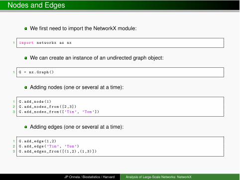
Nodes and Edges
We first need to import the NetworkX module:
1 import networkx as nx
We can create an instance of an undirected graph object:
1 G = nx.Graph()
Adding nodes (one or several at a time):
1 G.add_node (1)2 G.add_nodes_from ([2 ,3])3 G.add_nodes_from ([’Tim’, ’Tom’])
Adding edges (one or several at a time):
1 G.add_edge (1,2)2 G.add_edge(’Tim’, ’Tom’)3 G.add_edges_from ([(1 ,2) ,(1,3)])
JP Onnela / Biostatistics / Harvard Analysis of Large-Scale Networks: NetworkX

Nodes and Edges
List of all nodes (list of objects):
1 G.nodes()2 type(_)
List of all edges (list of tuples of objects):
1 G.edges()2 type(_)
Number of nodes:
1 G.number_of_nodes ()
Number of edges:
1 G.number_of_edges ()
JP Onnela / Biostatistics / Harvard Analysis of Large-Scale Networks: NetworkX

Nodes and Edges
We can also remove nodes and edges using similar methods:
1 G.remove_node (1)2 G.remove_nodes_from ([1 ,2])3 G.remove_edge (1,2)4 G.remove_edges_from ([(1 ,2), (2,3)])
To check for the existence of certain nodes or edges (returns True or False):
1 G.has_node (1)2 G.has_edge (1,2)
We can remove all nodes and all edges (the object G itself still remains):
1 G.clear()
JP Onnela / Biostatistics / Harvard Analysis of Large-Scale Networks: NetworkX

Nodes and Edges
Let’s use one of NetworkX’s network models to work with a slightly larger graph:
1 N = 100 # number of nodes2 k = 6 # number of nearest neighbors3 p = 0.05 # edge rewiring probability4 G = nx.watts_strogatz_graph(N, k, p)
List of neighbors of a given node:
1 G.neighbors (1)
There is another more direct and faster way to find the neighbors of a nodeNote: Use this only to read the dictionary; do not modify the dictionary directly
1 G[1]
{0: {}, 99: {}, 4: {}, 98: {}, 3: {}, 30: {}}Degree by definition is the number of neighbors a given node hasSince the neighbors() method returns a list, we can use its length to get degree:
1 len(G.neighbors (1))
But more simply we can just use
1 G.degree (1)
JP Onnela / Biostatistics / Harvard Analysis of Large-Scale Networks: NetworkX

Nodes and Edges
We can use the degree() method to find the degrees of all nodes:
1 G.degree ()
This returns a dictionary with node-degree as key-value pairs
Quiz: How do we get just a list of node degrees?
1 G.degree ().values ()2 sorted(G.degree ().values ())
The latter makes use of the built-in sorted() function to order the degrees fromlow to high
JP Onnela / Biostatistics / Harvard Analysis of Large-Scale Networks: NetworkX

Nodes and Edges
Exercise 1: Write a script that loops through each node and prints out node IDand node degree
0 6...
Exercise 2: Write a script that loops through each node and prints out node IDand a list of neighbor node IDs
0 [1, 2, 3, 97, 12, 98]...
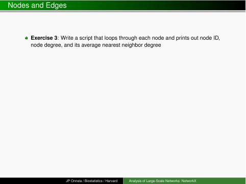
Exercise 3: Write a script that loops through each node and prints out node ID,node degree, and its average nearest neighbor degree
0 6 6.16666666667...
JP Onnela / Biostatistics / Harvard Analysis of Large-Scale Networks: NetworkX

Nodes and Edges
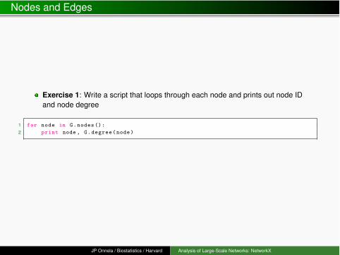
Exercise 1: Write a script that loops through each node and prints out node IDand node degree
1 for node in G.nodes():2 print node , G.degree(node)
JP Onnela / Biostatistics / Harvard Analysis of Large-Scale Networks: NetworkX
Nodes and Edges
Exercise 1: Write a script that loops through each node and prints out node IDand node degree
1 for node in G.nodes():2 print node , G.degree(node)
JP Onnela / Biostatistics / Harvard Analysis of Large-Scale Networks: NetworkX

Nodes and Edges
Exercise 2: Write a script that loops through each node and prints out node IDand a list of neighbor node IDs
1 for node in G.nodes():2 print node , G.neighbors(node)
JP Onnela / Biostatistics / Harvard Analysis of Large-Scale Networks: NetworkX

Nodes and Edges
Exercise 2: Write a script that loops through each node and prints out node IDand a list of neighbor node IDs
1 for node in G.nodes():2 print node , G.neighbors(node)
JP Onnela / Biostatistics / Harvard Analysis of Large-Scale Networks: NetworkX
Nodes and Edges
Exercise 3: Write a script that loops through each node and prints out node ID,node degree, and its average nearest neighbor degree
1 for node in G.nodes():2 cumdeg = 03 for neighbor in G.neighbors(node):4 cumdeg += G.degree(neighbor)5 print node , G.degree(node), float(cumdeg) / G.degree(node)
1 for node in G.nodes():2 if G.degree(node) > 0:3 cumdeg = 04 for neighbor in G.neighbors(node):5 cumdeg += G.degree(neighbor)6 print node , G.degree(node), float(cumdeg) / G.degree(node)
The first piece of code results in division by zero for isolated (degree zero) nodes,which leads to a run-time error
JP Onnela / Biostatistics / Harvard Analysis of Large-Scale Networks: NetworkX

Basic Network Properties
NetworkX provides a number of methods for computing network propertiesNote that the following are methods of the NetworkX module, not of graph objectsClustering coefficient characterizes the connectedness of a node’s neighbors:
ci =2ti
ki(ki � 1)
Here ti is the number of connections among the neighbors of node i, and ki is thedegree of node i
1 nx.clustering(G)2 nx.clustering(G,1)3 nx.clustering(G,[1,2,3,4])
Extract the subgraph induced by a set of nodes
1 g = nx.subgraph(G,[1,2,3,4,5,6])2 g.number_of_edges ()
Extract connected components (returns a list of lists of the nodes in connectedcomponents; the list is ordered from largest connected component to smallest)Note that the method works for undirected graphs only
1 nx.connected_components(G)
JP Onnela / Biostatistics / Harvard Analysis of Large-Scale Networks: NetworkX
Basic Network Properties
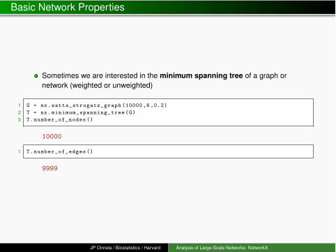
Sometimes we are interested in the minimum spanning tree of a graph ornetwork (weighted or unweighted)
1 G = nx.watts_strogatz_graph (10000 ,6 ,0.2)2 T = nx.minimum_spanning_tree(G)3 T.number_of_nodes ()
10000
1 T.number_of_edges ()
9999
JP Onnela / Biostatistics / Harvard Analysis of Large-Scale Networks: NetworkX

File Operations on NetworkX
NetworkX has methods for reading and writing network files
Two useful formats are edge lists and adjacency lists
Column separator can be either a space (default), comma, or something else
By default comment lines begin with the #-character
JP Onnela / Biostatistics / Harvard Analysis of Large-Scale Networks: NetworkX

File Operations on Edge Lists
Unweighted edge list is a text file with two columns: source targetWeighted edge list is a text file with three columns: source target dataReading edgelists happens with the following commands:
1 G = nx.read_edgelist("edgelist.txt")2 G = nx.read_edgelist("edgelist.txt", comments="#", delimiter=",", nodetype=int)3 G = nx.read_weighted_edgelist("edgelist_w.txt", comments="#", delimiter=",",
nodetype=int)4 G.edges()5 G.edges(data=True)
[(1, 2), (1, 3)][(1, 2, {’weight’: 5.0}), (1, 3, {’weight’: 5.0})]Edge lists can be written using the following commands:
1 nx.write_edgelist(nx.path_graph (4), "edgelist.txt", delimiter=’ ’)
0 1 {}...
1 nx.write_edgelist(nx.path_graph (4), "edgelist.txt", delimiter=’ ’, data=False)
0 1...
1 nx.write_weighted_edgelist(G, "edgelist_w.txt", delimiter=’ ’)
0 1 5.0...
JP Onnela / Biostatistics / Harvard Analysis of Large-Scale Networks: NetworkX

File Operations on Adjacency Lists
Adjacency lists are typically unweighted and have the following format:source target_1 target_2 target_3 ...
Reading adjacency lists:
1 G = nx.read_adjlist("adjlist.txt")2 G = nx.read_adjlist("adjlist.txt", comments=’#’, delimiter=’ ’, nodetype=int)
Writing adjacency lists can be done similarly:
1 G = nx.watts_strogatz_graph (100 ,6 ,0.2)2 nx.write_adjlist(G,"adjlist.txt")3 nx.write_adjlist(G,"adjlist.txt", delimiter=’ ’)
JP Onnela / Biostatistics / Harvard Analysis of Large-Scale Networks: NetworkX

Generating Random Graphs
NetworkX has some of the canonical random graphs readily implemented
Erdos-Rényi (ER) random graph (one of the implementations):
1 G_er = nx.erdos_renyi_graph (1000 , 0.15)
Watts-Strogatz (WS) random graph:
1 G_ws = nx.watts_strogatz_graph (1000, 3, 0.1)
Barabási-Albert (BA) random graph:
1 G_ba = nx.barabasi_albert_graph (1000 , 5)
Many others are available for creating, for example, Petersen graphs, Tuttegraphs, etc.
JP Onnela / Biostatistics / Harvard Analysis of Large-Scale Networks: NetworkX

Graph and Node attributes
Attributes (weights, labels, colors, etc.) can be attached to graphs, nodes, andedges
Graph attributes are useful if you need to deal with (are lucky enough to have)several graphs (e.g., in a longitudinal context)
1 G1 = nx.Graph(year =2004)2 G2 = nx.Graph(year =2006)3 G2.graph
{’year’: 2006}
1 G2.graph[’year’] = 2005
JP Onnela / Biostatistics / Harvard Analysis of Large-Scale Networks: NetworkX

Graph and Node Attributes
Node attributes can be used, for example, to represent demographic data (gender,etc.), or the status of a node in a dynamic process (susceptible, infectious, etc.)
1 G.add_node(1, sex = ’f’)2 G.add_node(2, sex = ’m’)3 G.add_nodes_from ([3,4,5,7], sex = ’f’)
List the nodes with and without attributes:
1 G.nodes()2 G.nodes(data=True)
[1, 2, 3, 4, 5, 7][(1, {’sex’: ’f’}), (2, {’sex’: ’m’}), (3, {’sex’: ’f’}), ... ]
JP Onnela / Biostatistics / Harvard Analysis of Large-Scale Networks: NetworkX

Graph and Node Attributes
We can look up node attributes
1 G.node2 G.node [1]
{1: {’sex’: ’f’}, 2: {’sex’: ’m’}, 3: {’sex’: ’f’}, ... }{’sex’: ’f’}
We can also modify node attributes
1 G.node [1][’status ’] = ’s’2 G.node [2][’status ’] = ’i’
Make sure to keep these distinct:
1 G.nodes() # method yielding a list of node IDs2 G.nodes(data=True) # method yielding a list of node IDs with node attributes3 G.node # dictionary of node attributes
JP Onnela / Biostatistics / Harvard Analysis of Large-Scale Networks: NetworkX

Edge Attributes
Edge attributes can be used to represent edge-based data characterizing theinteraction between a pair of nodes
For example, in a communication network consisting of cell phone calls, we coulduse the number of phone calls made between the two nodes over a period of time(n) and the total duration of phone calls over a period of time (d) as edge weights
1 G.add_edge(1, 2, n = 12, d = 3125)2 G.add_edge(1, 3, n = 9, d = 625)
List all edges with and without data
1 G.edges(data=True)2 G.edges()
[(1, 2, {’d’: 3125, ’n’: 12}), (1, 3, {’d’: 625, ’n’: 9})][(1, 2), (1, 3)]
JP Onnela / Biostatistics / Harvard Analysis of Large-Scale Networks: NetworkX

Edge Attributes
The short-cut syntax for accessing node attributes also works for edge attributes
1 G[1]
{2: {’d’: 3125, ’n’: 12}, 3: {’d’: 625, ’n’: 9}}
1 G[1][2]
{’d’: 3125, ’n’: 12}
Adding weighted edges (one or several at a time):
1 # add one weighted edge2 G.add_edge(1, 2, weight =1.3)3 G.add_weighted_edges_from ([(1, 2, 1.3)]) # results in "weight" as the key45 # add multiple weighted edges with a common weight6 G.add_edges_from ([(1, 2), (2, 3)], weight =1.3)78 # add multiple weighted edges with different weights9 G.add_weighted_edges_from ([(1, 2, 1.3), (1, 3, 4.1)])
[(1, 2, {’d’: 3125, ’n’: 12, ’weight’: 1.3}), (1, 3, {’d’: 625,’n’: 9, ’weight’: 4.1}), (2, 3, {’weight’: 1.3})]
JP Onnela / Biostatistics / Harvard Analysis of Large-Scale Networks: NetworkX
Edge Attributes
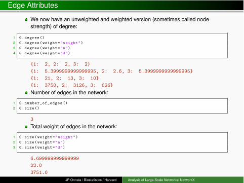
We now have an unweighted and weighted version (sometimes called nodestrength) of degree:
1 G.degree ()2 G.degree(weight="weight")3 G.degree(weight="n")4 G.degree(weight="d")
{1: 2, 2: 2, 3: 2}{1: 5.3999999999999995, 2: 2.6, 3: 5.3999999999999995}{1: 21, 2: 13, 3: 10}{1: 3750, 2: 3126, 3: 626}Number of edges in the network:
1 G.number_of_edges ()2 G.size()
3Total weight of edges in the network:
1 G.size(weight="weight")2 G.size(weight="n")3 G.size(weight="d")
6.69999999999999922.03751.0
JP Onnela / Biostatistics / Harvard Analysis of Large-Scale Networks: NetworkX

Exercise: Edge Overlap
We used the concept of edge overlap to examine the so-called weak tiehypothesis in “Structure and tie strengths in mobile communication networks” byJ.-P. Onnela, J. Saramaki, J. Hyvonen, G. Szabo, D. Lazer, K. Kaski, J. Kertesz,and A.-L. Barabasi, PNAS 104, 7332 (2007)
JP Onnela / Biostatistics / Harvard Analysis of Large-Scale Networks: NetworkX

Exercise: Edge Overlap
Write a function that computes the overlap Oij of an edge (i, j), defined as thenumber of neighbors the nodes adjacent to the edge have in common, divided bythe total number of neighbors the two nodes have combined:
Oij =nij
(ki � 1) + (kj � 1)� nij(1)
Here ki and kj are the degrees of nodes i and j, respectively, and nij is thenumber of neighbors the two nodes have in common
Hint: You will need to be able to find the degree of a given node, the neighbors ofa given node, and the intersection of the neighbors of two nodes. Sets might beuseful for this purpose.
JP Onnela / Biostatistics / Harvard Analysis of Large-Scale Networks: NetworkX

Exercise: Edge Overlap
Write a function that computes the overlap Oij of an edge (i, j), defined as thenumber of neighbors the nodes adjacent to the edge have in common, divided bythe total number of neighbors the two nodes have combined:
Oij =nij
(ki � 1) + (kj � 1)� nij
1 # overlap.py2 # Function for computing edge overlap , defined for non -isolated edges.3 # JP Onnela / May 24 201245 def overlap(H, edge):6 node_i = edge [0]7 node_j = edge [1]8 degree_i = H.degree(node_i)9 degree_j = H.degree(node_j)
10 neigh_i = set(H.neighbors(node_i))11 neigh_j = set(H.neighbors(node_j))12 neigh_ij = neigh_i & neigh_j13 num_cn = len(neigh_ij)14 if degree_i > 1 or degree_j > 1:15 return float(num_cn) / (degree_i + degree_j - num_cn - 2)16 else:17 return None
JP Onnela / Biostatistics / Harvard Analysis of Large-Scale Networks: NetworkX
Exercise: Edge Overlap
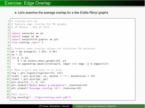
Let’s examine the average overlap for a few Erdos-Rényi graphs
1 # overlap_test.py2 # Explore edge overlap for ER graphs.3 # JP Onnela / May 24 201245 import networkx as nx6 import numpy as np7 import matplotlib.pyplot as plt8 from overlap import *9
10 # Compute some overlap values for different ER networks.11 ps = np.arange(0, 1.001 , 0.05)12 os = []13 for p in ps:14 G = nx.erdos_renyi_graph (100, p)15 os.append(np.mean([ overlap(G, edge) for edge in G.edges()]))1617 # Make a plot and save it to file.18 fig = plt.figure(figsize =(10, 10))19 line1 = plt.plot(ps, os, marker = "o", markersize = 10)20 line2 = plt.plot(ps, ps)21 plt.axis([0, 1, 0, 1])22 plt.xlabel("Erdos -Renyi p-parameter", fontsize =15)23 plt.ylabel("Average overlap <O>", fontsize =15)2425 #plt.show()26 fig.savefig("../ figs/overlap_test.pdf")
JP Onnela / Biostatistics / Harvard Analysis of Large-Scale Networks: NetworkX

Exercise: Edge Overlap
Figure: Average edge overlap hOi as a function of p for Erdos-Rényi networks. The figure wascomputed using N = 1000 for each network. The green line is the identity mapping and is shownfor reference.
JP Onnela / Biostatistics / Harvard Analysis of Large-Scale Networks: NetworkX

Exercise: Edge Overlap
Consider an edge (i, j) in an Erdos-Rényi graph
The probability for i to be connected to a node k, excluding node j is p; thereforethe probability for both of them to be connected to node k is p2
Therefore the expected number of common neighbors is (N � 2)p2
The expected (average) degree is given by (N � 1)p
This yields the following expression for edge overlap:
Oij =(N � 2)p2
2(N � 1)p� 2� (N � 2)p2
Taking the limit N ! 1 this leads to
Oij =Np2
2Np� 2�Np2=
p
2� 2/Np� p=
p
2� p
JP Onnela / Biostatistics / Harvard Analysis of Large-Scale Networks: NetworkX

Exercise: Edge Overlap
Figure: Plot of expected overlap p/(2 � p) in an Erdos-Rényi network as a function of p.
JP Onnela / Biostatistics / Harvard Analysis of Large-Scale Networks: NetworkX

Network Visualization
NetworkX uses the Matplotlib module for some simple network visualizationsLet’s start with an Erdos-Rényi network with N = 100 and p = 0.11
Note that the actual drawing is deferred until the call to show()
1 import networkx as nx2 import matplotlib.pyplot as plt34 G = nx.erdos_renyi_graph (100 ,0.11)5 plt.figure(figsize =(10 ,10))6 nx.draw(G)7 plt.axis("tight")8 plt.show()
JP Onnela / Biostatistics / Harvard Analysis of Large-Scale Networks: NetworkX

Network Visualization
We can print the figure directly to file by capturing the figure object and then usingthe savefig method
Figure format will be specified by the file extension
Possible to specify complete paths (absolute or relative)
1 import networkx as nx2 import matplotlib.pyplot as plt34 G = nx.erdos_renyi_graph (100 ,0.11)5 fig = plt.figure(figsize =(10 ,10))6 nx.draw(G, with_labels = False)7 plt.axis("tight")8 fig.savefig("../ figs/vis2.pdf")
JP Onnela / Biostatistics / Harvard Analysis of Large-Scale Networks: NetworkX

Network Visualization
Sometimes we want to keep the node positions fixed
It is possible to compute the node locations separately, resulting in a dictionary,which can then be used subsequently in plotting
1 import networkx as nx2 import matplotlib.pyplot as plt34 G1 = nx.erdos_renyi_graph (100 ,0.01)5 G2 = nx.erdos_renyi_graph (100 ,0.02)6 G3 = nx.erdos_renyi_graph (100 ,0.04)7 G4 = nx.erdos_renyi_graph (100 ,0.08)89 fig = plt.figure(figsize =(10 ,10))
10 pos = nx.spring_layout(G4 ,iterations =500)11 plt.subplot (2,2,1)12 nx.draw(G1 , pos , node_size =40, with_labels=False); plt.axis("tight")13 plt.subplot (2,2,2)14 nx.draw(G2 , pos , node_size =40, with_labels=False); plt.axis("tight")15 plt.subplot (2,2,3)16 nx.draw(G3 , pos , node_size =40, with_labels=False); plt.axis("tight")17 plt.subplot (2,2,4)18 nx.draw(G4 , pos , node_size =40, with_labels=False); plt.axis("tight")19 fig.savefig("../ figs/vis3.pdf")
JP Onnela / Biostatistics / Harvard Analysis of Large-Scale Networks: NetworkX

Network Visualization
Figure: Erdos-Rényi networks with different values for the p-parameter using fixed node locations.
JP Onnela / Biostatistics / Harvard Analysis of Large-Scale Networks: NetworkX