Analysis of Indian monsoon daily rainfall on subseasonal …blyon/REFERENCES/P87.pdf2 5100100...

QUARTERLY JOURNAL OF THE ROYAL METEOROLOGICAL SOCIETYQ. J. R. Meteorol. Soc. 134: 875–887 (2008)Published online 27 May 2008 in Wiley InterScience(www.interscience.wiley.com) DOI: 10.1002/qj.254

Analysis of Indian monsoon daily rainfall on subseasonal tomultidecadal time-scales using a hidden Markov model

A. M. Greene,a* A. W. Robertsona and S. Kirshnerb

a International Research Institute for Climate and Society, Palisades, New York, USAb University of Alberta, Edmonton, Canada

ABSTRACT: A 70-year record of daily monsoon-season rainfall at a network of 13 stations in central western India isanalyzed using a 4-state homogeneous hidden Markov model. The diagnosed states are seen to play distinct roles in theseasonal march of the monsoon, can be associated with ‘active’ and ‘break’ monsoon phases and capture the northwardpropagation of convective disturbances associated with the intraseasonal oscillation. Interannual variations in station rainfallare found to be associated with the alternation, from year to year, in the frequency of occurrence of wet and dry states; thismode of variability is well correlated with both all-India monsoon rainfall and an index characterizing the strength of the ElNino Southern Oscillation. Analysis of low-passed time series suggests that variations in state frequency are responsible forthe modulation of monsoon rainfall on multidecadal time-scales as well. Copyright 2008 Royal Meteorological Society

KEY WORDS climate diagnosis; precipitation; statistical modelling

Received 23 January 2007; Revised 12 March 2008; Accepted 26 March 2008

1. Introduction

Owing to both its meteorological and economic signifi-cance, the Indian monsoon has been studied intensively(e.g. Gadgil, 2003; Webster et al., 1998; Abrol, 1996;Rai, 2005; Gadgil and Kumar, 2006; Gadgil and Gadgil,2006). In the present work, daily monsoon rainfall at asmall network of stations is decomposed using a hiddenMarkov model (HMM). The HMM is utilized here as adiagnostic tool; this is a necessary step if such a model iseventually to be deployed for precipitation downscalingor simulation (Hughes et al., 1999; Bellone et al., 2000).To the best of our knowledge HMMs have not previ-ously been deployed in this regional setting; this rendersthe present investigation both novel and of interest gener-ally, with regard to the diagnostic utility of such modelsin the monsoon domain.

The HMM associates observed patterns of daily rainfallwith a small set of ‘hidden states’, which proceedin time as a first-order Markov process (Hughes andGuttorp, 1994; Norris, 1997). It may be considered aparsimonious description of the raw rainfall observationsor, alternatively, as a method of data reduction, bywhich the essential structural attributes of the complexobservational data are represented by a small, thereforemore comprehensible, set of parameters.

The HMM also provides a simple means of generatingsynthetic precipitation series that have some of thestatistical properties (including spatial covariance) of

* Correspondence to: A. M. Greene, International Research Institute forClimate and Society, Palisades, NY 10964, USA.E-mail: [email protected]

the data to which it is fitted. Here, however, thisis not the goal; in particular, the model employedincludes only seasonal-mean transition probabilities, andis thus incapable of simulating the rise and fall of theseasonal cycle. However, once the hidden states areidentified, their progression in time can be recovered,and intraseasonal variability thereby diagnosed. It is thisdiagnosis that lies at the core of the present work.

Monsoon rainfall is highly variable both temporallyand spatially, in particular at the scale of individualweather stations. The HMM is fitted directly to thedaily station data without any filtering or gridding, yetis shown to capture characteristic features of rainfallvariability across a broad range of time scales. Thissuggests the existence of some mechanism that linksvariations occurring on these different scales. It hasbeen noted, for example, that the ‘active’ and ‘break’phases that characterize subseasonal monsoon variability‘add up’ to produce interannual variations (Gadgil andAsha, 1992; Gadgil, 1995; Goswami and Xavier, 2003;Goswami, 2005). It is thus of interest to see whether suchaggregation might also play a role in decadal monsoonfluctuations.

The link between the monsoon and the El Nino South-ern Oscillation (ENSO) has also received attention (Ras-musson and Carpenter, 1983; Shukla, 1987; Krishna-murthy and Goswamy, 2000; Kumar et al., 2006), thegeneral consensus being that strong El Nino events havetended to be associated with weak monsoons, at leastup until the late 1970s (Kumar et al., 1999). This link-age is explored here through canonical correlation anal-ysis (CCA), applied to the occurrence frequencies of the

Copyright 2008 Royal Meteorological Society

876 A. M. GREENE ET AL.

diagnosed states and the station rainfall data. CCA is thenextended, to examine multidecadal variability.

Section 2 describes the datasets employed and Sec-tion 3 some climatological characteristics of the data. TheHMM is discussed in Section 4, while Section 5 exam-ines the hidden states in terms of associated atmosphericcomposites. Sections 6, 7 and 8 deal with intrasea-sonal, interannual and multidecadal variability, respec-tively; a discussion and summary follow, in Sections 9and 10.

2. Data

A 70-year record of daily rainfall at 13 stations, from theGlobal Daily Climatology Network (GDCN; Legates andWillmott, 1990), constitutes the primary dataset. Thesestations were initially chosen to match, by name andlocation, a group of records for 1973–2004 that had beenobtained from the Global Surface Summary of Day Data(NCDC, 2002), with the thought that the two datasetscould be combined. However, given the reasonablylong GDCN data series and their relative freedom frommissing values, as well as potential inhomogeneity issues,we restrict our attention to this 70-year record.

The GDCN data span the years 1901–1970, with astation average of only 11 missing days out of 8540,and no station missing more than 29 days. The stationsthemselves are listed in Table I and locations shownin Figure 1. Although some regions, notably the east-ern coast, are not sampled, atmospheric circulation com-posites (discussed in Section 5) suggest that this net-work captures enough of the spatio-temporal variabil-ity of the precipitation field for the large-scale featuresof the monsoonal circulation to be quite well inferred.Interannual variations in mean station rainfall are wellcorrelated (r = 0.86) with the Indian Summer MonsoonRainfall (ISMR) index, an average of June–September

Table I. Stations whose records are utilized here.

No. ISTA Stationname

Lat( °N)

Lon( °E)

P(R) I

1 5010600 Ahmadabad 23.06 72.63 0.41 15.02 5100100 Veraval 20.90 70.36 0.43 11.03 5150100 Rajkot 22.30 70.78 0.35 13.74 5171200 Surat 21.20 72.83 0.56 15.35 11170400 Indore 22.71 75.80 0.54 13.16 11180800 Jabalpur 23.20 79.95 0.58 17.47 12040300 Aurangabad 19.85 75.40 0.49 10.28 12190100 Poona 18.53 73.85 0.58 7.29 12230300 Sholapur 17.66 75.90 0.41 10.9

10 19070100 Bikaner 28.00 73.30 0.17 12.111 19131300 Jaipur 26.81 75.80 0.36 12.112 22021900 Delhi 28.58 77.20 0.30 16.013 23351200 Lucknow 26.75 80.88 0.43 17.1

No. = station number used in Figure 1(a).ISTA = station ID as provided in the dataset.P(R) = climatological rainfall occurrence probability.I = mean intensity (rainfall amount on wet days).

rainfall over approximately 300 stations (Sontakke et al.,1993).

Atmospheric circulation fields are derived from theNational Centers for Environmental Prediction–NationalCenter for Atmospheric Research (NCEP–NCAR)reanalysis (Kalnay et al., 1996). Comparisons weremade between composites derived from this dataset andfrom the European Centre for Medium-Range WeatherForecasts reanalysis (ERA-40; Uppala, 2001). Thosefrom the latter product were found to be somewhatnoisier, perhaps owing to the shorter usable data length(The period of overlap with the rainfall data is abouthalf as long for ERA-40.) The NCEP–NCAR data weretherefore utilized.

(a) (b)

80°70° 90°60°

10°

20°

30°

10°

20°

30°

80°70° 90°60°

15 mm

10 mm

5 mm9

8

23

4

1 5 6

1011

12

131000

1000

500

500

500

500

500500

50005000

00

0.25

0.5

0.75

98

2 47

31 5 6

1011

12

13

0

Figure 1. Climatological (a) occurrence probability and (b) mean daily intensity (mm) for Jun–Sep 1901–1970. Numbers within station circlesidentify stations listed in Table I.

Copyright 2008 Royal Meteorological Society Q. J. R. Meteorol. Soc. 134: 875–887 (2008)DOI: 10.1002/qj

ANALYSIS OF INDIAN MONSOON DAILY RAINFALL 877

3. Climatology

3.1. Rainfall – spatial distribution

Figures 1(a) and 1(b) illustrate mean Jun–Sep climato-logical rainfall occurrence probabilities and mean dailyintensities (rainfall amounts on wet days), respectively,over the network. Topographic contours from the GLOBEdigital elevation model (Hastings and Dunbar, 1998) arealso shown. Both probabilities and intensities (also givenin Table I), are computed conditional on a minimum dailyrainfall amount of 0.1 mm, the minimum non-zero valuerecorded in the dataset.

In Figure 1, high probability and intensity values alongthe western coast reflect onshore flow, as shown inFigure 5(a), impinging on coastal orography (Gadgil,2003). This orography can also produce sharp gradientsin intensity, as is the case with station 8. The high valuesat station 6, on the other hand, arise from convectivesystems propagating northwestward from the Bay ofBengal, reaching across the classical ‘monsoon zone’,a broad belt extending across the mid-section of thesubcontinent (Figure 5a in Gadgil, 2003). The patternsshown in Figures 1(a, b) are quite consistent with ahigh-resolution (1°) dataset from the India MeteorologicalDepartment (IMD; Rajeevan et al., 2006), includingthe low probabilities and intensities to the north andnorthwest, (e.g. station 10, lying in arid Rajasthan),the high intensities at stations 6 and 13 in the mainmonsoon zone, and the southeast to northwest intensitygradient in going from stations 7–9 toward stations1–4. Absolute amounts do differ somewhat, with thestation data showing generally both higher occurrenceprobabilities and mean daily intensities than enclosinggrid boxes in the IMD product. The former may result

from the masking of gridded values below 0.1 mm, thelatter from grid-box averaging.

3.2. Rainfall – seasonal cycle

Figures 2(a,b) illustrate the climatological seasonal cyclefor rainfall occurrence frequency and mean daily intensityfor each of the 13 stations, using pentads. Both variablesexhibit a decided seasonal cycle at all stations. Station 10again stands out for its relatively low occurrence prob-abilities, although it clearly participates in the seasonalcycle. It is less of an outlier in terms of mean intensity;this can be seen as well in Figure 1.

3.3. Circulation

Figure 5(a) shows mean climatological Jun–Sep horizon-tal winds at 850 mb and the 500 mb vertical velocity (ω)from the NCEP–NCAR reanalysis, for 1951–1970. Sev-eral well-known features of the monsoon circulation areevident in the plot, including the cross-equatorial Somalijet along the coast of Africa, the southwesterly to westerlyflow in the Arabian sea, and ascending motion (ω < 0)concentrated in maxima in the eastern Arabian Sea andcentral Bay of Bengal (Xie and Arkin, 1996; Goswami,2005).

4. Model description

4.1. Basic structure and assumptions

The HMM factorizes the joint distribution of historicaldaily rainfall amounts recorded on a network of stationsin terms of a few discrete states, by making two

0.5

1.0

1.5

2.0

2.5

3.0

3.5

Jun 1–Sep 30(pentads)

Occ

urre

nce

freq

(da

ys/p

enta

d)

Jun 1–Sep 30(pentads)

Inte

nsity

, mm

/day

Sta1Sta2Sta3Sta4Sta5Sta6Sta7Sta8Sta9Sta10Sta11Sta12Sta13

(a) (b)

1015

05

5 10 15 20 5 10 15 20

Figure 2. Climatological seasonal cycle of (a) occurrence frequency (days pentad−1) and (b) mean daily intensity (mm) for the 13-station dataset,1901–1970. Occurrence is conditional on a threshold of 0.1 mm.



conditional independence assumptions: first, that therainfall on a given day depends only on the state activeon that day, and second, that the state active on agiven day depends only on the previous day’s state. Thelatter assumption corresponds to the Markov property;the states are considered ‘hidden’ because they are notdirectly observable.

The state-associated rainfall patterns comprise a prob-ability distribution function (PDF) for daily rainfall foreach of the stations. In the present instance these arethree-component mixtures, consisting of a delta func-tion to represent zero-rainfall days and two exponentialsrepresenting rainfall intensity. Mixed-exponential distri-butions have been found effective in the representation ofdaily precipitation (Woolhiser and Roldan, 1982). Dailyrainfall, conditional on state, is represented as

p(Rmt = r|St = i) =

pim0 r = 0,C∑

c=1

pimcλimce−λimcr r > 0,

(1)

where indices i, m and c refer to state, station and mixturecomponent, respectively, the pimc are weights and t istime. In the summation, C = 2, i.e. two exponentialsare utilized. Note that while rainfall at each stationis characterized by a PDF that is both station- andstate-specific, the PDFs for all stations are coupled bystate, as per the i subscripts in Equation (1). Thus, theHMM accounts for spatial dependence in the data. Thereare HMM variants that model spatial dependence inmore detail (Kirshner et al., 2004), but we forgo theadditional complexity involved in favour of a more easilyinterpreted model. Robertson et al. (2004, 2006) give amore complete description of the HMM.

4.2. Model selection and fitting

The number of states to be modelled must be speci-fied a priori; differing objectives may lead to differingchoices in this regard. Use of a small number of statesfacilitates diagnosis and model comprehensibility, theobject of this study, while a larger number might be moresuitable for the generation of synthetic data. Models hav-ing three, four, five and eight states were examined indetail. Of these, the three-state model was determinedto be suboptimal, particularly in relating the diagnosedstates to the propagating convective disturbances charac-teristic of the intraseasonal oscillation (ISO, Section 6.3).On the other hand, the five-state model does not addmuch to the descriptions already present with four statesand begins to exhibit ‘state splitting’, the subdivision ofattributes among states. Examination of the eight-statemodel confirms the tendency for complexity, but not nec-essarily clarity, to increase with the number of states.The Bayesian Information Criterion (Schwarz, 1978) wasapplied to fitted models having up to 20 states, (Figure 3)and indicates that overfitting does not occur when asmany as 10 states are modelled. For the illustrative pur-poses that are primary here, a model having four hidden

states was thus selected. We show in the following sec-tions that this model provides a physically meaningfuldescription of the monsoon and its variability across awide range of time-scales.

Parameter estimation was performed by the maxi-mum likelihood approach, using the iterative expec-tation–maximization (EM) algorithm (Dempster et al.,1977; Ghahramani, 2001). The algorithm was initialized30 times from random starting points, the run utilizedbeing that with the highest log-likelihood. Estimationwas performed using the Multivariate NonhomogeneousHidden Markov Model Toolbox, developed by one ofthe authors (Kirshner, http://www.cs.ualberta.ca/∼sergey/MVNHMM/).

4.3. Representation in terms of states

Figure 4 shows rainfall occurrence probabilities and meanintensities for the 4-state model, the former derived fromthe pim0 parameter in Equation (1), the latter from themean values and weights of the mixed-exponential dis-tributions. The four states exhibit distinctly different pat-terns for both variables: state 4, which might be charac-terized as the ‘dry’ state, shows small occurrence proba-bilities, and mean intensities that are small to moderate atall stations, while state 3, the ‘wet’ state, has relativelyhigh occurrence probabilities and intensities. State 1 isalso rather wet but shows a substantial southwest to north-east gradient in mean intensity, while state 2 exhibits anorth to south gradient in both occurrence probability andmean intensity.

4.4. Transition matrix

From a mechanistic (or generative) point of view, theHMM transition matrix provides the stochastic ‘engine’that drives the system from state to state with the progres-sion of days. Alternatively, and more importantly for ourpurposes, the matrix can be regarded as descriptive, sum-marizing the temporal dependence of the observations inprobabilistic form. The entry in row i, column j gives theconditional probability of an i –j transition, i.e. the prob-ability that tomorrow’s state will be j , given that today’sis i. The transition matrix for the 4-state HMM is shown

4.35

4.38

4.41

4.44

4.47

10 12 14 16 18 202

Number of states

BIC

(x

105 )

864

Figure 3. Bayesian information criterion (BIC) for models havingdiffering numbers of hidden states.



10°

20°

30°

0.25

0.5

0.75

(a)

70° 80° 90° 70° 80° 90° 70° 80° 90° 70° 80° 90°

10°

20°

30°

5 mm

10 mm

20 mm

(b)

(c)

(d)

(e)

(f)

10°

20°

30°

(g)

10°

20°

30°

(h)

Figure 4. (a) Occurrence probabilities and (b) mean daily intensities (mm) from the 4-state model, for state 1. (c,d), (e,f) and (g,h) are as (a,b),but for states 2, 3 and 4, respectively. Values are computed conditional on a daily amount of at least 0.1 mm. The legend in the leftmost panel

applies to all plots on that row.

in Table II. Note that the estimated 3–4 and 4–3 prob-abilities are both null (actually non-zero, but at least 7orders of magnitude smaller than the other values in thetable); in fact, no direct transitions between these twostates occur. This suggests that some dynamical processhas been encoded by the HMM, such that abrupt changesbetween the intense endmember conditions representedby these two states are unlikely to occur in nature.

The largest values in the transition matrix lie alongthe leading diagonal. Since these are the ‘self-transition’probabilities (i.e. probabilities of remaining in the respec-tive states from day to day), this feature signals a ten-dency, for all the states, to persist beyond the lengthof the sampling interval (one day). It is this tendencythat accounts for the horizontally banded appearance ofFigure 6(a), the most-likely state sequence (Section 6.1).

The values shown in Table II are time-invariant, andin essence represent mean transition probabilities forthe entire Jun–Sep season. As will be seen, however,

Table II. Transition matrix for the 4-state HMM. ‘From’states occupy the rows, ‘to’ states the columns. Thus e.g. the

probability of a transition from state 2 to state 4 is 0.056.

‘To’ state

1 2 3 4

1 0.798 0.031 0.087 0.083‘From’ 2 0.059 0.776 0.109 0.056state 3 0.160 0.018 0.823 0.000

4 0.022 0.101 0.000 0.876

there is a pronounced seasonal cycle in the relativefrequency of occurrence of the various states, implyingthat in actuality the probabilities must be temporallymodulated. This would clearly present a problem if itwas desired to simulate the rise and fall of the seasonalcycle, since static transition probabilities can produceonly stationary rainfall series. However, once the stateshave been diagnosed, their relative frequency over thecourse of the season, and thus the seasonal cycle, as itexists in the observed rainfall series, can be determined.This is discussed in more detail in Section 6.

5. Atmospheric correlates

It is of interest to see how the modelled states arerelated to the large-scale circulation, since the latter pro-vides a primary control on rainfall. Figures 5(b–e) showcomposited anomalies (with respect to the climatologyshown in Figure 5(a)) for states 1–4, respectively, forthe 4-state HMM.

Generation of these composites requires several steps.First, the raw daily rainfall values must be expressedin terms of the hidden states they represent. This isaccomplished here by means of the Viterbi algorithm(Section 6), which returns a ‘most-likely’ sequence ofstates, given the state definitions and transition matrix.Each day in the rainfall record is thus identified withits associated state. The days diagnosed as representingeach of the states are then collected, with all thedays representing state 1 placed in one group, the daysrepresenting state 2 in a second group, and so on. The



12090

40

−0.14 −0.12 −0.1 −0.08 −0.06 −0.04 −0.02 0 0.02 0.04 0.06 0.08 0.1 0.12 0.14

6030Eq

10

20

30

(a)

19 m s−1

4 m s−1

−0.04 −0.032 −0.024 −0.016 −0.008 0 0.008 0.016 0.024 0.032 0.04

120906030Eq

40

10

20

30

120906030

120906030Eq

40

10

20

30

120906030

(b) (c)

(d) (e)

Pa s−1

Pa s−1

Figure 5. (a) Horizontal winds at 850 mb (vectors, m s−1) and 500 mb vertical velocity (colours, Pa s−1) for the Jun–Sep mean climatology for1951–1970. (b)–(e) show anomalies with respect to (a), for states 1–4, respectively.

composites are formed by taking the arithmetic averageof the wind and vertical velocity fields for each of thesegroups, then subtracting the mean Jun–Sep climatology(shown in Figure 5(a)) to produce anomalies.

State 3 (Figure 5(d)), the wet state, is seen to be asso-ciated with an amplification of the mean seasonal pattern,along with landward displacements of the two centres ofascending motion that straddle the subcontinent. Anoma-lous cyclonic circulation is present over these centers.There is also anomalous onshore flow from the ArabianSea, as well as an anticyclonic circulation to the south-west of the Indian peninsula. These features are consistentwith the high occurrence probabilities and intensities on

the western coast, extending toward the northeast, thatcharacterize this state (Figures 4(e,f)). In addition, themore or less zonal band of anomalous ascending motioncan be identified with the often-described ‘monsoontrough’ (e.g. Rao, 1976). Here, this band extends broadlyin a northwestward direction from the Bay of Ben-gal, lying squarely over the monsoon zone as identifiedby Gadgil (2003). This atmospheric configuration alsocorresponds well with the dominant mode of intrasea-sonal variability identified by Annamalai et al. (1999)via empirical orthogonal function (EOF) analysis, andassociated with the ‘active’ monsoon phase (Goswami,2005).



The composite for state 4 (Figure 5(e)), the ‘dry’ state,is opposite in sense to that of state 3, with anomalousdescent over much of the subcontinent, and anticycloniccirculation anomalies where state 3 presents cyclonicones. This pattern is consistent with the lower occurrenceprobabilities and intensities shown in Figures 4(g,h).

State 1 exhibits higher occurrence probabilities thanstate 3 for some stations in the northeastern part of thedomain; the band of anomalous ascending motion seenin the corresponding composite (Figure 5(b)), althoughconfigured somewhat differently than in state 3, canstill be seen to correspond to the classical monsoontrough. However, the mean intensities here show astrong gradient (Figure 4(b)), with values increasingfrom southwest to northeast. In the composite we seeanomalous anticyclonic circulation centrally located inthe Arabian Sea, while a single centre of anomalousascent occurs near the northeastern part of the domain,near the Himalayan escarpment. Thus, high pressurebrings dry conditions to the coastal stations, while theanomalous ascent is located in a position consistent withhigher inland rainfall intensities.

Finally, state 2 (Figure 5(c)) shows anomalous east-erly inflow from the Bay of Bengal, resembling in thissense the dry state. State 2 is also opposed to state 1 (cf.Figure 5(b)), in that there is now anomalous cyclonicactivity, with associated rising motion, near the south-west coast, while the north central region shows anoma-lous descent and anticyclonic circulation. These proper-ties, like those of the other composites, are reflected inthe maps of occurrence probability and mean intensity(Figures 4(c,d)).

Broadly speaking, the circulation anomalies associatedwith states 1 and 2 can be said to be similar to thoseassociated with 3 and 4, respectively, but weaker, andwith the regions of strongest anomalous ascent or descentdisplaced to the north. States 1 and 3, with anomalousascending motion over the subcontinent, and in particularthe monsoon zone, may both be considered ‘wet’, whilestate 2, with its anomalous descending motion, showsstronger affinities to the dry state (state 4), most clearlyin the northern part of the domain.

Among the questions that naturally arise from inspec-tion of these figures is that of the relationship betweenthe diagnosed states and the wet and dry intraseasonal-scale phenomena known as ‘active’ and ‘break’ phasesof the monsoon. This question is taken up in Section 6,along with some other aspects of intraseasonal variabil-ity, as viewed through the prism of state decomposition.The rainfall patterns associated with the diagnosed statesappear, in any event, to correspond quite sensibly withknown large-scale monsoon-related circulation regimes(Gadgil, 2003).

6. Intraseasonal variability: Breaks and ISO

6.1. Viterbi sequence

Once the parameters of the HMM have been estimated,the most likely daily sequence of states can be determined

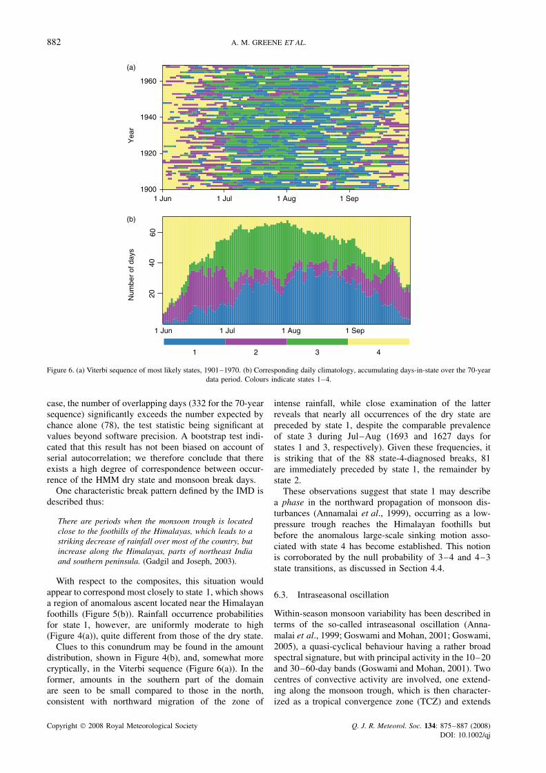
using the Viterbi algorithm (Forney, 1978), a dynamicprogramming scheme. The Viterbi sequence, whichexpresses the time evolution of rainfall patterns over theentire data period in terms of the hidden states, is shownfor the 4-state model in Figure 6(a). Figure 6(b) showsthe climatological sequence for 1901–1970, accumulat-ing days-in-state over the 70 years.

Figures 6(a,b) reveal a systematic progression in stateoccurrence over the course of the monsoon season.During the first half of June, state 4 (the dry state)dominates, while during the core of the rainy seasonstates 1 and 3 assume primary importance. State 2 plays aquasi-transitional role, first appearing as a bridge betweendry and wet conditions in late June, almost disappearingduring the wettest part of the season, then returningin September, with increasing representation toward theend of that month. After mid-September the dry stateonce again becomes dominant. Figure 6(b) also revealsa subtle evolution of precipitation patterns during thecore rainy season, with July favouring state 3 but a shifttoward state 1 in August.

Over the 70-year data period the four states occur on anaverage of 34, 22, 30 and 36 days, respectively, duringthe 122-day Jun–Sep season, with standard deviations10.3, 7.9, 11.8 and 15.2 days, indicating considerableinterannual variability. Variability on longer time-scalesis also suggested by Figure 6(a).

6.2. Monsoon breaks

Figures 6(a,b) both show clearly the dominance of state 4during the early and late stages of the monsoon. This statealso occurs sporadically during the Jul–Aug core of therainy season, however, suggesting a possible associationwith monsoon breaks. Gadgil and Joseph (2003) providea listing of breaks for 1901–1989, as defined by rainfallthresholds in the western and eastern sectors of themonsoon zone. These thresholds were chosen in orderthat there be a good correspondence between breaks sodefined and breaks as identified in a broad range of otherstudies, so their listing can be considered representative.

Gadgil and Joseph identify an average of 8.8 breakdays during Jul–Aug for 1901–1970, while the averagenumber of dry-state days is 7.9. Standard deviations of theGadgil and Joseph and state 4 series are 6.3 and 7.4 days,respectively. There are nine years in which the Gadgil andJoseph listing shows no break days, and in each of theseyears there are no occurrences of the dry state. However,there are five additional years in which the dry state doesnot occur, in which Gadgil and Joseph do indicate breaks.Interannual variations in the number of break and state-4 days are highly correlated (r = 0.76, significant at the0.0001 level in a one-sided test).

Correspondence between the particular days whenbreaks are diagnosed and those days when the Viterbialgorithm identifies state 4 can be expressed in the formof a 2 × 2 contingency table and evaluated by meansof the χ2 test, either summing over years, or consider-ing the entire dataset as a single long sequence. In either



Num

ber

of d

ays

1 Jun 1 Jul 1 Aug 1 Sep

2040

60

1 Jun 1 Sep1 Aug1 Jul1900

1940

1920

1960

(a)

(b)

Yea

r

1 2 3 4

Figure 6. (a) Viterbi sequence of most likely states, 1901–1970. (b) Corresponding daily climatology, accumulating days-in-state over the 70-yeardata period. Colours indicate states 1–4.

case, the number of overlapping days (332 for the 70-yearsequence) significantly exceeds the number expected bychance alone (78), the test statistic being significant atvalues beyond software precision. A bootstrap test indi-cated that this result has not been biased on account ofserial autocorrelation; we therefore conclude that thereexists a high degree of correspondence between occur-rence of the HMM dry state and monsoon break days.

One characteristic break pattern defined by the IMD isdescribed thus:

There are periods when the monsoon trough is locatedclose to the foothills of the Himalayas, which leads to astriking decrease of rainfall over most of the country, butincrease along the Himalayas, parts of northeast Indiaand southern peninsula. (Gadgil and Joseph, 2003).

With respect to the composites, this situation wouldappear to correspond most closely to state 1, which showsa region of anomalous ascent located near the Himalayanfoothills (Figure 5(b)). Rainfall occurrence probabilitiesfor state 1, however, are uniformly moderate to high(Figure 4(a)), quite different from those of the dry state.

Clues to this conundrum may be found in the amountdistribution, shown in Figure 4(b), and, somewhat morecryptically, in the Viterbi sequence (Figure 6(a)). In theformer, amounts in the southern part of the domainare seen to be small compared to those in the north,consistent with northward migration of the zone of

intense rainfall, while close examination of the latterreveals that nearly all occurrences of the dry state arepreceded by state 1, despite the comparable prevalenceof state 3 during Jul–Aug (1693 and 1627 days forstates 1 and 3, respectively). Given these frequencies, itis striking that of the 88 state-4-diagnosed breaks, 81are immediately preceded by state 1, the remainder bystate 2.

These observations suggest that state 1 may describea phase in the northward propagation of monsoon dis-turbances (Annamalai et al., 1999), occurring as a low-pressure trough reaches the Himalayan foothills butbefore the anomalous large-scale sinking motion asso-ciated with state 4 has become established. This notionis corroborated by the null probability of 3–4 and 4–3state transitions, as discussed in Section 4.4.

6.3. Intraseasonal oscillation

Within-season monsoon variability has been described interms of the so-called intraseasonal oscillation (Anna-malai et al., 1999; Goswami and Mohan, 2001; Goswami,2005), a quasi-cyclical behaviour having a rather broadspectral signature, but with principal activity in the 10–20and 30–60-day bands (Goswami and Mohan, 2001). Twocentres of convective activity are involved, one extend-ing along the monsoon trough, which is then character-ized as a tropical convergence zone (TCZ) and extends



from the northern Bay of Bengal northwestward overthe Indian landmass, and a second lying in the IndianOcean between 0° and 10 °S. The detailed time evolutionof the ISO is apparently complex, consisting, accordingto Goswami and Mohan (2001) of

. . . fluctuations of the TCZ between the two locations andrepeated propagation from the southern to the northernposition. . .

Annamalai et al. (1999) in fact refer to the northwardpropagation of convective activity as ‘non-periodic’. Inany event, the two ‘phases’ of the ISO, i.e. with con-vective centres of action located over the two preferredzones, are to be associated with the active and breakphases of the monsoon, the northerly location correspond-ing to the active phase.

In the light of this description, states 1 and 3(Figures 5(b,d)) can clearly be identified with the activephase, while state 4 and, to a lesser extent, state 2 maybe identified with the break phase. However, for the lat-ter two states there is little in the vertical motion fieldsouth of the Equator (region not shown in these plots)to suggest deep convection. Thus, while some aspectsof a correspondence between the state composites andthe ISO seem reasonably clear, the structure of the drystate does not appear to correspond in all particulars tothe canonical break-phase description of Goswami andMohan (2001).

The HMM is sensitive not only to differing patterns ofrainfall occurrence and intensity per se, but also to therelative frequency with which these patterns are man-ifest. Thus, a distinctive pattern that occurred on onlya very small number of days would tend to be sub-sumed into a state having greater representation amongthe observations. A propagating pattern would then mostlikely find expression in terms of its more temporallypersistent phases. Ghil and Robertson (2002) considerthe relationship between persistence, atmospheric statesand oscillatory modes in the context of a ‘wave-particleduality’. The modes, or ‘slow phases’ in their terminol-ogy, are thus more likely to be captured by the statedescriptions.

6.4. Propagation of convective disturbances

We focus here on the Jul–Aug core of the wet sea-son. During these months the monsoon is fully active,the dry periods at the beginning of June and end ofSeptember being excluded. Transition probabilities forJul–Aug, estimated from the Viterbi sequence, are shownin Table III (cf. Table II, which applies to the entireJun–Sep season, and where transitions to the dry statefrom states 1 and 2 are considerably more likely). Weconsider the off-diagonal elements in this array, fromwhich most likely sequences of states may be deduced.Exclusion of elements on the main diagonal is equiva-lent to considering only transitions from one state to adifferent state, thus ignoring self-transitions. Attention is

thereby directed to the temporal patterns of intraseasonalvariability, rather than the daily transitions.

The most likely sequence, thus defined, varies accord-ing to which state is taken as the starting point, butif we think of the ISO as described by Goswami andMohan (2001), i.e. as an alternation between two cen-tres of convective activity (with propagation from southto north), we can think of a complete ‘cycle’ as extend-ing from break to break – a break occurring when thelocus of convection lies to the south of the Equator.Beginning with a break (state 4), the most likely statesequence is then 4–2–3–1. Figure 7 shows compos-ites of 850 mb relative vorticity corresponding to thewind fields of Figures 5(b–e). Viewed in the 4–2–3–1sequence, the plots show a northward progression of theband of positive vorticity, beginning, in state 4, at thesouthern extremity of the subcontinent. This would beconsistent with the northward-propagating disturbancesdescribed by Goswami and Mohan (2001).

The Markov chain, of course, follows some mixtureof all the paths permitted by the transition matrix; thus,there is considerable stochastic variability in the actualprogression of states. Nevertheless, the 4–2–3–1 patternis frequently found intact in the Viterbi sequence.

In summary, much in the state composites is consis-tent with the ISO, as it has been variously described.However, it should be remembered that the states arenot regular snapshots in time, constrained to follow oneanother in a deterministic order. Furthermore, the datahave not been filtered to retain only ISO-band variability,and thus contain information about all time-scales.

6.5. Other aspects of intraseasonal variability

From Table III it can be seen that another ‘preferred’sequence consists of an alternation between states 1and 3, and also that the 1–3 transition probability isabout twice that of 1–4. An alternation between states 1and 3 is consistent with the maintenance of generallyheavy precipitation during Jul–Aug, and the less frequentexcursions to state 4 with the occasional occurrence ofbreaks. Stochastic switching between these two transi-tional modes would be consistent with the intermittentcharacter of northward propagation associated with theISO, as described by both Annamalai et al. (1999) andGoswami (2005).

A feature of interest in Figure 6(b) involves the shiftin dominance, during the peak Jul–Aug period, from

Table III. July–August transition probabilities.

‘To’ state

1 2 3 4

1 0.847 0.014 0.091 0.047‘From’ 2 0.066 0.763 0.158 0.013state 3 0.132 0.009 0.859 0.000

4 0.050 0.106 0.000 0.844



−20

0

0

12

2

Eq

40

10

20

30

−1

−1

0

0 0

0

0

1

1 11

2

2

4

−7−3

−1−1

−1−1

−1 −1

1

1 1

1 1

3

5 7

120906030

Eq

40

10

20

30−3

−1

−1

−1

−1−1

−1

1

1

1

33

3

3

3

5

7

120906030

(a) (b)

(c) (d)

Figure 7. Relative vorticity anomaly composites (10−6 s−1) for the 4-state model: (a)–(d) show states 1–4, respectively.

state 3 toward state 1. This may reflect an increasingtendency toward the dry state (nearly always preceded bystate 1 but never by state 3), and ultimately the end ofthe rainy season itself, as July turns to August. Increasingpredominance of state 1 as the season matures may alsobe viewed as a tendency, with time, for convection tooccur preferentially in the more northerly reaches of thecountry.

7. Interannual variations – Influence of ENSO

The four-state model comprises two ‘wet’ and two ‘dry’states, with states 3 and 4 the more intense in these twocategories, respectively, and 1 and 2 the more attenuated.Over the course of a full season, the number of daysspent in each of the states can thus signal relatively wetor dry years; the unfolding in time of these variationsconstitutes what we would call interannual variability,but now expressed in terms of frequency of occurrence(FO) of the model’s hidden states. These occurrencefrequencies, which apply to the station network as whole,may in turn be thought of as representing interannualvariations in the large-scale circulation. (Indeed, this hasbeen demonstrated in Section 5.) On the other hand,the states are related to the station rainfall through thestructure of the HMM. Thus, state FO links the largespatial scale of the circulation fields with the smallscales of station rainfall. This linkage is explored in whatfollows.

The number of days in a given year assigned toeach of the states may be computed from the Viterbisequence. Correlation coefficients for the four FO seriesthus obtained and the NINO3.4 index (Barnston et al.,1994) are –0.18, –0.16, –0.45 and 0.56 for states 1to 4, respectively. The first two of these values are not

statistically significant (two-sided test), even at a level of0.10, while the latter two prove significant at better than0.001 (on 68 degrees of freedom, dof) This indicates atendency for El Nino (La Nina) years to be associatedwith increased FO of the dry (wet) state, consistent withthe sense of the historical ENSO-monsoon relationship.The NINO3.4 index is also anticorrelated with theISMR (r = −0.63), indirectly linking FO to this broad-scale metric. These relationships confirm the large-scalecharacter of state FO, as would be expected from theresults of Section 5.

The relationship between FO and station rainfall cannotbe considered for each of the states separately, becauseFO need not (indeed, cannot) vary independently amongstates. In addition, there exists the possibility that within-state variation (changes in the character of the states),if systematic, could cause station rainfall variations todiverge from what variations in FO alone would lead us toexpect. Canonical correlation analysis (CCA; e.g. Wilks,2006) offers a means of addressing these potentiallyconfounding aspects of the FO–rainfall linkage, andis thus employed here in order to characterize thatrelationship.

CCA identifies pairs of patterns across two fields, suchthat the temporal correlation between members of a pairis maximized. The original variables can be projectedonto the diagnosed patterns to estimate the degree towhich the actual behaviour of the fields is captured bythem. In the CCA performed here, the method of Barnettand Preisendorfer (1987), in which the original data arefirst expressed, or ‘filtered’, in terms of EOFs, is utilized.Moron et al. (2008) have performed a similar analysis,as part of an investigation of Senegalese rainfall.

The two ‘fields’ analyzed, each having annual values,are the state FO series and the mean daily station rainfall



amounts. Initially, all series are filtered to remove decadaland longer-period variability. This is done by first gen-erating smoothed versions of the series, using 11-yearrunning means. These smoothed versions are then sub-tracted from the original series, leaving the shorter-periodvariations as a residual. The Kolmogorov–Smirnov testdid not lead to a rejection of the null hypothesis of nor-mality for any of the resulting state or station series; CCAwas thus applied without any transformation of variables.

Figures 8(a,b) illustrate, respectively, the FO andstation rainfall patterns corresponding to the leadingmode of covariability. The correlation between the twocanonical variates for this mode is 0.92, while the patternsthemselves explain 48% of the variance of the FO fieldand 33% of the variance of the rainfall amounts. A MonteCarlo significance test that involves scrambling the timeindices while retaining spatial field structure indicates thatthe correlation value is significant at better than 0.001.The next two modes also have significant correlationcoefficients and explain 14% and 12% of the rainfallvariance, respectively. Thus, the leading CCA mode onsubdecadal time-scales consists of an alternation betweenstates 3 and 4, the wet and dry states, coupled to a rainfallpattern in which mean seasonal amounts change in thesame sense at all stations, becoming wetter (drier) whenstate 3 (4) predominates. From the HMM perspective,then, ENSO modulates monsoon rainfall through theagency of the state frequencies, producing lower (higher)counts for state 3 (4) in El Nino years, vice versa for LaNina years.

The leading canonical variate time series for the FOseries is well correlated with the ISMR index (r =0.81, significant at better than 0.0001). This can betaken as additional confirmation that the HMM statedecomposition, based on only a 13-station network, hascaptured patterns that are implicitly descriptive of thisbroadly representative index.

Potential utility of the HMM as a predictive downscal-ing tool was tested for the interannual case by attempt-ing to forecast precipitation over the station network foreach year, using a CCA fitted to the remaining datayears. The four FO series were utilized as predictors,and all three significantly correlated CCA modes, which

together explain 60% of the station rainfall variance, wereutilized. The correlation between observed and cross-validated forecast station rainfall series was 0.49±0.13(1σ ), and the mean RMS error 1.7 mm, or 30% of theseasonal mean daily amount (averaged over both stationsand years). For the stations with higher correlations thisrepresents potentially useful forecast skill. It should bekept in mind, however, that these measures assume aperfect forecast of the state frequencies, which will notbe the case in practice.

8. Multidecadal behaviour

Figure 9 shows the smoothed FO time series, in whichsubdecadal variability is suppressed. Series for states 1and 2 do not exhibit marked long-term trends, althoughdecadal variations are evident. Series for states 3 and4 trend in opposite directions, however, the formerincreasing. This tendency, of states 3 and 4 to vary inopposite senses, also characterizes decadal variations, andsuggests similarities with the interannual case.

Figures 8(c,d) show the first canonical patterns for thesmoothed data, which are seen to be similar to thosefor the interannual series. The first three correlations arealso significant (at 0.001) in this case, and explain 52%,24% and 7% of the station rainfall variance, respectively.The smoothed ISMR is also well correlated with the firstFO canonical variate (r = 0.85, p value of 0.015 for atwo-way test on 5 dof), so an appreciable fraction of thedecadal variance can be related to the state frequencies,even though the states themselves are diagnosed withrespect to daily data. Thus, it appears that decadalvariations of the ISMR amount in part to an aggregation,over many years, of wet and dry states. This can beviewed as an extension of the intraseasonal–interannualrelation identified by Goswami and Mohan (2001).

9. Discussion

The homogeneous HMM is utilized here as a diagnos-tic tool, and provides a compact description of daily

−10

−5

0

5

10

1 2 3 4

(a)

70° 80° 90°

10°

20°

30°

0.5 mm

1mm

2 mm

(b)

−4

−2

0

2

4

1 2 3 4

(c)

70° 80° 90°

10°

20°

30°

0.1 mm

0.5 mm

1 mm

(d)

Day

s in

sta

te

Day

s in

sta

te

Figure 8. First canonical patterns for state FO for the subdecadal series: (a) days in state and (b) mean daily rainfall amount (mm). (c,d) are as(a,b), but for the low-passed series. In (d) the single negative value (most easterly station) is shaded.



1920 1940 19601900

40

50

20

30

State 1State 2State 3State 4

Day

s in

sta

te

Year

Figure 9. Time evolution of filtered state occurrence frequencies. Series shown are 11-year moving averages. Units are days-in-state during the122-day Jul–Sep monsoon season.

rainfall variability over the station network. The rela-tionships detailed, between variations in FO of the diag-nosed states, station rainfall distributions and variousmonsoon features (large-scale atmospheric flow, ISO, all-India monsoon rainfall, ENSO interaction, longer-periodvariability) indicate that this description contains muchinformation about real physical processes.

Well-defined atmospheric modes corresponding to thestates are consistent with both the state rainfall patternsand the large-scale structure of the monsoon. This corre-spondence may owe something to the fact that the mon-soon is a large-scale phenomenon, whose modes might beaccessible in this way from any similar network meetingsome minimal sampling requirement.

It was shown that year-to-year fluctuations in the firstCCA mode, representing inverse variations in the FOof states 3 and 4, play an important role in monsoonvariations on even decadal time-scales. The possibilitythat there are, in addition, low-frequency modes ofvariability whose expression is similar to the behaviourthat is here attributed to the aggregation of wet and drystates over decade-length periods cannot be ruled out.However, such modes are not amenable to discoverythrough the agency of the HMM.

10. Summary and conclusions

A homogeneous hidden Markov model is applied to dailyIndian monsoon rainfall on a network of 13 stations inwest central India, for the years 1901–1970. The HMMassociates patterns of rainfall received at the stations witha set of hidden states, that progress in time as a first-orderMarkov process. For the purposes of the present work, amodel having four hidden states is found to be optimal,in that it captures sufficient detail to represent essentialfeatures of monsoon variability, while retaining adequateinterpretive simplicity for the purposes of the presentexposition. To the best of our knowledge, application of

a statistical model of this type in the Indian monsoondomain has not previously been attempted.

The diagnosed states were found to play distinct rolesin the seasonal march of the monsoon, and the associatedatmospheric composites to correspond sensibly with staterainfall characteristics. Episodes of dry-state occurrenceduring the peak rainy season were shown to correspondwell with independently diagnosed monsoon breaks,while detailed analysis of the time evolution of ‘mostlikely’ states revealed a correspondence with phases inthe northward propagation of convective disturbancescharacteristic of the ISO. This evidence lends credenceto the HMM representation of monsoon spatio-temporalvariability, and suggests that such models may also finduse in other monsoon-dominated circulation regimes.

On interannual time scales, a strong relationshipbetween ENSO and monsoon rainfall is found for theperiod under study. Canonical correlation analysis iden-tifies a primary mode in which the occurrence frequenciesof the driest and wettest states vary in opposing senses.Both all-India monsoon rainfall and a typical ENSO indexare found to project strongly onto this mode, implyingthat the state frequencies are strongly coupled to both sea-sonal rainfall totals and ENSO. These relationships per-sist on decadal time-scales, suggesting that long-periodfluctuations in monsoon rainfall can ultimately be linkedto interannual variations in state FO. This diagnosis,which has not been made previously, differs from that ofMoron et al., (2008) with respect to Senegalese rainfall,in which decadal variability was found to be primarily aconsequence of within-state variation, while interannualvariability was more strongly influenced by FO.

A preliminary experiment utilizing the diagnosed FOseries as predictors suggested that the HMM may proveuseful in this regional setting as a statistical downscalingtool, although better quantification awaits further investi-gation. A related application, in an area of research thathas received increasing attention of late, is the gener-ation of weather-within-climate data, in the context oflong-range climate change studies. The model validation



presented here represents an important step toward therealization of these applications.

Acknowledgements

We appreciate the helpful advice and comments offeredby many staff members at the IRI, including Lisa God-dard, Vincent Moron and Michael Tippet, by PadhraicSmyth of the University of California, Irvine and by threeanonymous reviewers. This research was supported byUS Department of Energy grant DE-FG02-02ER63413.

References

Abrol IP. 1996. India’s agriculture scenario. Pp 19–25 in ClimateVariability and Agriculture. Abrol YP, Gadgil S, Pant GB (eds).Narosa: New Delhi.

Annamalai H, Slingo JM, Sperber KR, Hodges K. 1999. The meanevolution and variability of the Asian summer monsoon: Comparisonof ECMWF and NCEP-NCAR reanalyses. Mon. Weather Rev. 127:1157–1186.

Barnett TP, Preisendorfer R. 1987. Origins and levels of monthly andseasonal forecast skill for United States surface air temperaturesdetermined by canonical correlation analysis. Mon. Weather Rev.115: 1825–1850.

Barnston AG, van den Dool HM, Rodenhuis DR, Ropelewski CR,Kousky VE, O’Lenic EA, Livezey RE, Zebiak SE, Cane MA,Barnett TP, Graham NE, Ji M, Leetmaa A. 1994. Long-leadseasonal forecasts – Where do we stand? Bull. Am. Meteorol. Soc.75: 2097–2114.

Bellone E, Hughes JP, Guttorp P. 2000. A hidden Markov model fordownscaling synoptic atmospheric patterns to precipitation amounts.Clim. Res. 15: 1–12.

Dempster AP, Laird NM, Rubin DR. 1977. Maximum likelihood fromincomplete data via the EM algorithm. J. R. Stat. Soc. B39: 1–38.

Forney GD Jr. 1978. The Viterbi algorithm. Proc. IEEE 61: 268–278.Gadgil S. 1995. Climate change and agriculture: An Indian perspective.

Current Sci. 69: 649–659.Gadgil S. 2003. The Indian monsoon and its variability. Ann. Rev. Earth

Planet. Sci. 31: 429–467. Doi:10.1146/annurev.earth.31.100901.141251.

Gadgil S, Asha G. 1992. Intraseasonal variation of the summermonsoon. Part I: Observational aspects. J. Meteorol. Soc. Jpn. 70:517–527.

Gadgil S, Gadgil S. 2006. The Indian Monsoon, GDP and agriculture.Econom. Pol. Weekly 41: 47, 4887–4895.

Gadgil S, Joseph PV. 2003. On breaks of the Indian monsoon. Proc.Indian Acad. Sci. (Earth Planet. Sci.) 112: 529–558.

Gadgil S, Kumar KR. 2006. The Asian monsoon – Agriculture andeconomy. Pp 651–683 in The Asian Monsoon. Bin Wang (ed.)Springer: Berlin.

Ghahramani Z. 2001. An introduction to hidden Markov modelsand Bayesian networks. Int. J. Pattern Recogn. 15: 9–42.DOI:10.1142/S0218001401000836.

Ghil M, Robertson A. 2002. ‘Waves’ vs. ‘particles’ in the atmosphere’sphase space: A pathway to long-range forecasting? Proc. Nat. Acad.Sci. 99(suppl. 1): 2493–2500.

Goswami BN. 2005. South Asian monsoon. Pp 19–61 in Intraseasonalvariability in the atmosphere–ocean climate system. Lau WKM,Waliser DE (eds.) Springer: Berlin.

Goswami GN, Ajaya Mohan RS. 2001. Intraseasonal oscillations andinterannual variability of the Indian summer monsoon. J. Climate14: 1180–1198.

Goswami BN, Xavier PK. 2003. Potential predictability and extended-range prediction of Indian summer monsoon breaks. Geophys. Res.Lett. 30: DOI:10.1029/2003GL017810.

Hastings DA, Dunbar PK. 1998. Development and assessmentof the Global Land One-km Base Elevation digital elevationmodel (GLOBE). Int. Soc. Photogramm. Remote Sens. Arch. 32:218–221.

Hughes JP, Guttorp P. 1994. A class of stochastic models for relatingsynoptic atmospheric patterns to regional hydrologic phenomena.Water Resour. Res. 30: 1535–1546.

Hughes JP, Guttorp P, Charles SP. 1999. A non-homogeneous hiddenMarkov model for precipitation occurrence. J. R. Stat. Soc. C 48:15–30. DOI:10.1111/1467–9876.00136.

Kalnay E, Kanamitsu M, Kistler R, Collins W, Deaven D, Gandin L,Iredell M, Saha S, White G, Woollen J, Zhu Y, Chellah M, EbisuzakiW, Higgins W, Janowiak J, Mo KC, Ropelewski C, Wang J, LeetmaaA, Reynolds R, Jenne R, Joseph D. 1996. The NCEP/NCAR 40-yearreanalysis project. Bull. Am. Meteorol. Soc. 77: 437–471.

Kirshner S, Smyth P, Robertson AW. 2004. ‘Conditional Chow-Liutree structures for modeling discrete-valued vector time series’. Uni-versity of California, School of Information and Computer Science:Technical Report ICU–ICS 04-04. http://iri.columbia.edu/∼awr/papers/tr0404.pdf.

Krishnamurthy V, Goswami BN. 2000. Indian Monsoon-ENSOrelationship on interdecadal timescale. J. Climate 13: 579–595.

Kumar KK, Rajagopalan B, Cane MA. 1999. On the weakeningrelationship between the Indian monsoon and ENSO. Science 284:2156–2159.

Kumar KK, Rajagopalan B, Hoerling M, Bates G, Cane MA. 2006.Unraveling the mystery of Indian monsoon failure during El Nino.Science 314: 115–119.

Legates DR, Willmott CJ. 1990. Mean seasonal and spatial variability ingauge-corrected global precipitation. Int. J. Climatol. 10: 111–127.

Moron V, Robertson AW, Ward MN, Ndiaye O. 2008. Weather typesand rainfall over Senegal. Part I: Observational analysis. J. Climate21: 266–287.

NCDC. 2002. Data documentation for dataset 9618, Global summaryof the day. NOAA National Climatic Data Center: Asheville.http://www4.ncdc.noaa.gov/ol/documentlibrary/datasets.html.

Norris JR. 1997. Markov chains. Cambridge University Press:Cambridge, UK.

Rai S. 2005. Monsoon still helps push India’s economy. Int. HeraldTribune http://www.iht.com/articles/2005/06/03/news/india.php.

Rajeevan M, Bhate J, Kale JD, Lal B. 2006. High-resolution dailygridded rainfall data for the Indian region: Analysis of break andactive monsoon spells. Current Sci. 91: 296–306.

Rao YP. 1976. Southwest monsoon. Meteorological Monograph, IndiaMeteorological Dept: Poona, India.

Rasmusson EM, Carpenter TH. 1983. The relationship between easternequatorial Pacific sea surface temperatures and rainfall over India andSri Lanka. Mon. Weather Rev. 111: 517–528.

Robertson AW, Kirshner S, Smyth P. 2004. Downscaling of dailyrainfall occurrence over northeast Brazil using a hidden Markovmodel. J. Climate 17: 4407–4424.

Robertson AW, Kirshner S, Smyth P, Charles SP, Bates BC. 2006.Subseasonal-to-interdecadal variability of the Australian monsoonover North Queensland. Q. J. R. Meteorol. Soc. 132: 519–542.

Schwarz G. 1978. Estimating the dimension of a model. Ann. Stat. 6:461–464.

Shukla J. 1987. Interannual variability of monsoons. Pp 399–464 inMonsoons, Fein JS, Stephens PL (eds.) Wiley: New York.

Sontakke NA, Pant GB, Singh N. 1993. Construction of all-Indiasummer monsoon rainfall series for the period 1844–1991. J.Climate 6: 1807–1811.

Uppala SM. 2001. ‘ECMWF Reanalysis 1957–2001, ERA-40’.Workshop on reanalysis 5–9 Nov 2001. ERA-40 Project ReportSeries No. 3, ECMWF, Reading, UK.

Webster PJ, Magana VO, Palmer TN, Shukla J, Tomas RA, YanaiM, Yasunari T. 1998. Monsoons: Processes, predictability, and theprospects for prediction. J. Geophys. Res. 103: C7, 14 451–14 510.

Wilks DS. 2006. Statistical methods in the atmospheric sciences.International Geophysics Series 91, Academic Press: Burlington,MA, USA.

Woolhiser DA, Roldan J. 1982. Stochastic daily precipitation models2. A comparison of distributions of amounts. Water Resour. Res. 18:1461–1468.

Xie P, Arkin P. 1996. Analyses of global monthly precipitationusing gauge observations, satellite estimates, and numerical modelpredictions. J. Climate 9: 840–858.

Zucchini W, Guttorp P. 1991. A hidden Markov model for space-timeprecipitation. Water Resour. Res. 27: 1917–1923.


Analysis of Indian monsoon daily rainfall on subseasonal …blyon/REFERENCES/P87.pdf2 5100100...

Documents

Transcript of Analysis of Indian monsoon daily rainfall on subseasonal …blyon/REFERENCES/P87.pdf2 5100100...