
Analysis of Hyperelastic Materials with MECHANICA – Theory ... · PDF fileAnalysis of...
72
Analysis of Hyperelastic Materials with MECHANICA – Theory and Application Examples – Dr.-Ing. Roland Jakel, PTC Presentation for the 2 nd SAXSIM | Technische Universität Chemnitz 27. April 2010 | Rev. 1.0
Transcript of Analysis of Hyperelastic Materials with MECHANICA – Theory ... · PDF fileAnalysis of...

Analysis of Hyperelastic Materials with MECHANICA – Theory and Application Examples –Dr.-Ing. Roland Jakel, PTCPresentation for the 2nd SAXSIM | Technische Universität Chemnitz27. April 2010 | Rev. 1.0
Table of Contents (1)
Part 1: Theoretic background information (4-35)
Review of Hooke’s law for linear elastic materials (5-6)
The strain energy density of linear elastic materials (7-8)
Hyperelastic material (9-11)
Material laws for hyperelastic materials (12-17)
© 2010 PTC2
About selecting the material model and performing tests (18-19)
Implementation of hyperelastic material laws in Mechanica (20-22)
Defining hyperelastic material parameters in Mechanica (23-26)
Test set-ups and specimen shapes of the supported material tests (27-31)
The uniaxial compression test (32-33)
Stress and strain definitions in the Mechanica LDA analysis (34-36)

Table of Contents (2)
Part 2: Application examples (36-63)
A test specimen subjected to uniaxial loading (38-44)
A volumetric compression test (45-50)
A planar test (51-58)
Influence of the material law (59-64)
© 2010 PTC3
Appendix
PTC Simulation Services Introduction (66-69)
Dictionary Technical English-German (70-71)
Acknowledgement
Thanks to Tad Doxsee and Rich King from Mechanica R&D for the helpful support!

Part 1
Theoretic Background Information
© 2010 PTC4
Review of Hooke’s law for linear elastic materials (1)
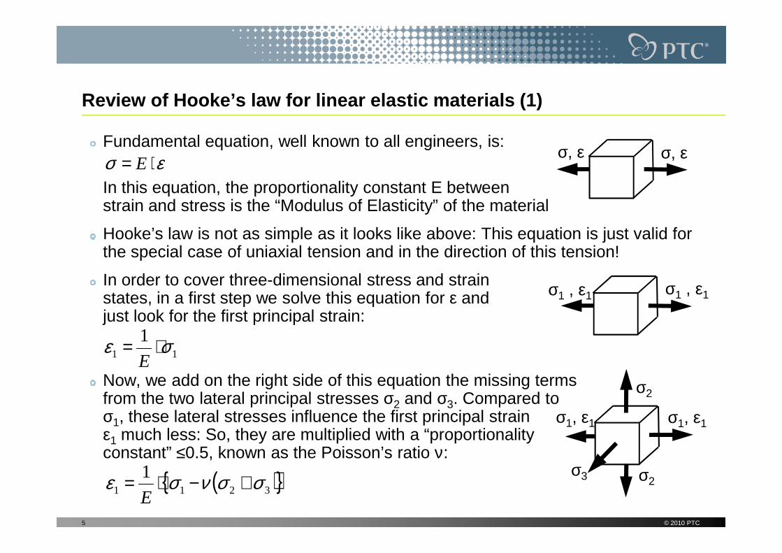
Fundamental equation, well known to all engineers, is:
In this equation, the proportionality constant E betweenstrain and stress is the “Modulus of Elasticity” of the material
Hooke’s law is not as simple as it looks like above: This equation is just valid for the special case of uniaxial tension and in the direction of this tension!
In order to cover three-dimensional stress and strain
εσ ⋅= Eσ, εσ, ε
In order to cover three-dimensional stress and strain states, in a first step we solve this equation for ε and just look for the first principal strain:
Now, we add on the right side of this equation the missing terms from the two lateral principal stresses σ2 and σ3. Compared to σ1, these lateral stresses influence the first principal strain ε1 much less: So, they are multiplied with a “proportionality constant” ≤0.5, known as the Poisson’s ratio ν:
© 2010 PTC5
11
1 σε ⋅=E
( ){ }3211
1 σσνσε +−⋅=E
σ1 , ε1σ1 , ε1
σ1, ε1
σ2
σ3 σ2
σ1, ε1

Review of Hooke’s law for linear elastic materials (2)
If we do the same in the other two orthogonal principal directions, we obtain the general formulation of Hooke’s law:
( ){ }
( ){ }
( ){ }
3122
3211
1
1
1
σσνσε
σσνσε
σσνσε
+−⋅=
+−⋅=
+−⋅=
E
E
σ1, ε1
σ2, ε2
Remark:If we also take into account thermal strains, we obtain in direction 1 for example
Hence, the well known simple equation to calculate a stress-free length change from heating up a material
( ){ } ϑασσνσε ∆⋅++−⋅= 3211
1
E
ϑα ∆⋅⋅=∆ ll
The limits of the Poisson ratio ν are:
– ν=0: no influence of lateral stresses to the strain (no lateral contraction)
– ν=0.5: incompressible material, means there is no volume change under loads (of course there is usually a big change in shape under loads!)
– ν=0.2…0.3: typical values for linear elastic material like ceramic & metal
© 2010 PTC6
( ){ }2133
1 σσνσε +−⋅=E σ3, ε3 is just another special case of Hooke’s law with σi=0
(all directions stress free):
ϑα ∆⋅⋅=∆ ll
ϑαε ∆⋅=∆=l
l

The strain energy density of linear elastic materia ls (1)
When loading and unloading a linear elastic material, we “drive” along the same straight line in the stress-strain characteristic curve:
σ
The strain energy density W of such a material is expressed as the half value of the double dot product of stress tensor S and strain tensor E:
To explain it more simply for listeners who are not familiar with tensor operations, let’s have a look at a simple spring: Every engineer knows its spring energy is
with K=spring stiffness and ∆l=spring elongation
© 2010 PTC7
ε
2
2
1lKEspring ∆=
ESW ⋅⋅=2
1
The strain energy density of linear elastic materia ls (2)
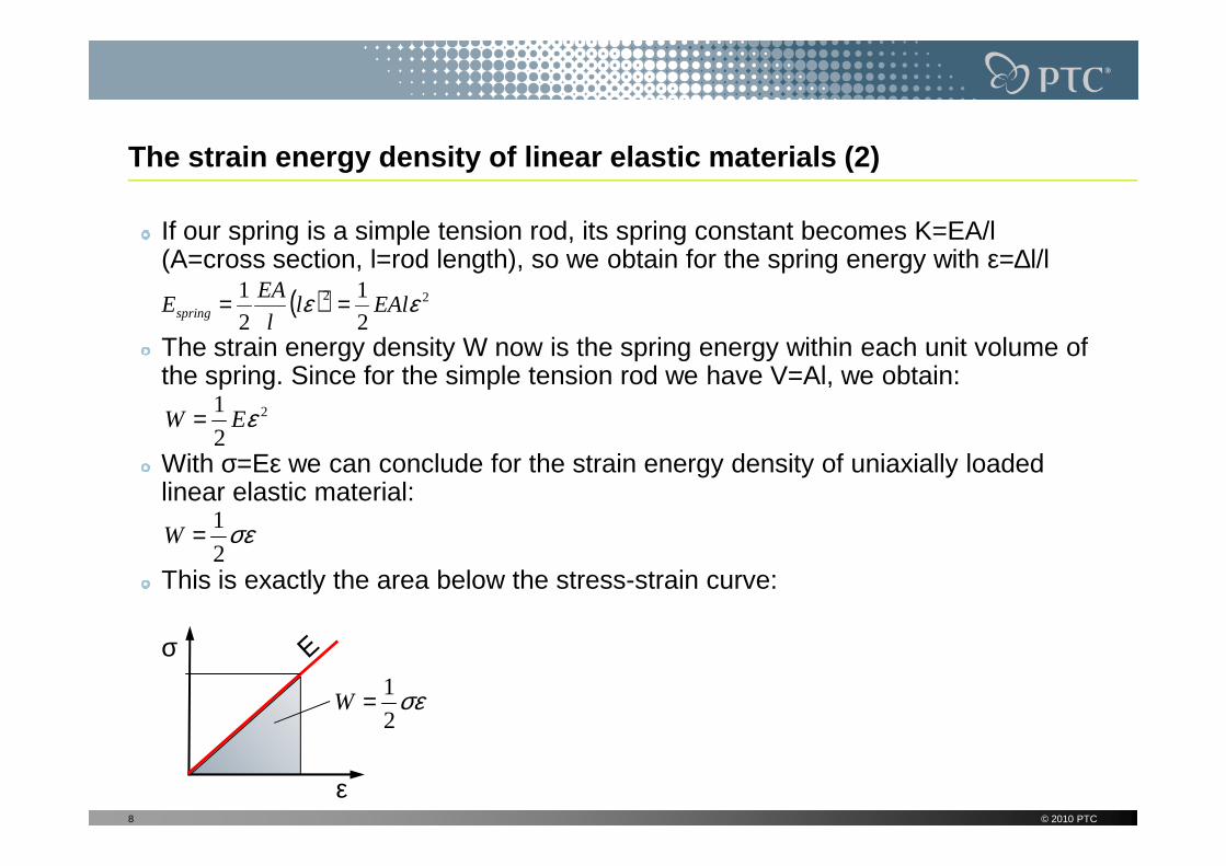
If our spring is a simple tension rod, its spring constant becomes K=EA/l (A=cross section, l=rod length), so we obtain for the spring energy with ε=∆l/l
The strain energy density W now is the spring energy within each unit volume of the spring. Since for the simple tension rod we have V=Al, we obtain:
( ) 22
2
1
2
1 εε EAlll
EAEspring ==
2
2
1 εEW =
With σ=Eε we can conclude for the strain energy density of uniaxially loaded linear elastic material:
This is exactly the area below the stress-strain curve:
© 2010 PTC8
σ
ε
2
σε2
1=W
σε2
1=W

Hyperelastic material (1)
Hyperelastic and linear elastic material:
A hyperelastic material is still an elastic material, that means it returns to it's original shape after the forces have been removed
Hyperelastic material also is Cauchy-elastic, which means that the stress is determined by the current state of deformation, and not the path or history of deformation
The difference to linear elastic Material is,that in hyperelastic material the stress-strain relationship derives from a strain energy density function, and not a constant factor
This definition says nothing about the Poisson's ratio or the amount of deformation that a material will undergo under loading
However, often elastomers are modeled as hyperelastic. Hyperelasticity may also be usedto describe biological materials, like tissue
© 2010 PTC9
σ
ε
Hyperelastic material behavior
Hyperelastic material (2)
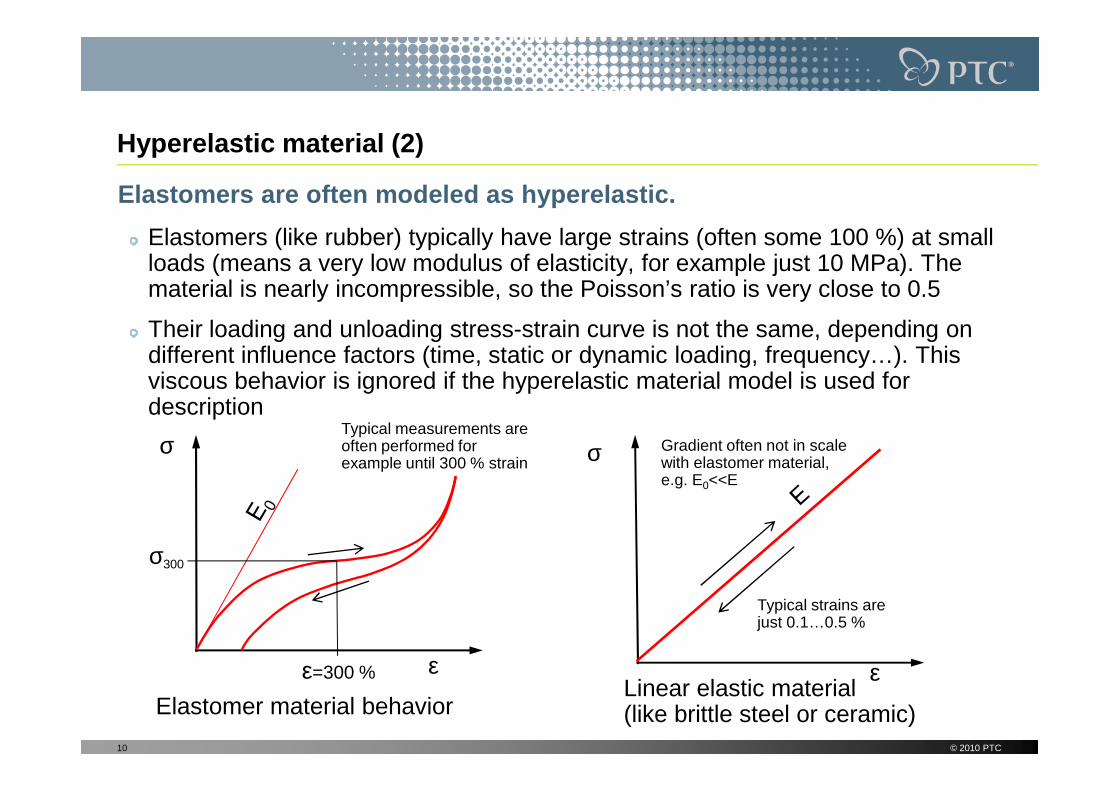
Elastomers are often modeled as hyperelastic.
Elastomers (like rubber) typically have large strains (often some 100 %) at small loads (means a very low modulus of elasticity, for example just 10 MPa). The material is nearly incompressible, so the Poisson’s ratio is very close to 0.5
Their loading and unloading stress-strain curve is not the same, depending on different influence factors (time, static or dynamic loading, frequency…). This viscous behavior is ignored if the hyperelastic material model is used for descriptiondescription
© 2010 PTC10
σ
ε
σ
εε=300 %
σ300
Elastomer material behaviorLinear elastic material(like brittle steel or ceramic)
Typical measurements are often performed for example until 300 % strain
Gradient often not in scale with elastomer material, e.g. E0<<E
Typical strains are just 0.1…0.5 %

Hyperelastic material (3)
Elastomer material in comparison with metals and pla stics:
Energy-elasticity: Loading changes the distance of the atoms within the lattice of the metal and so increases the internal energy. When unloading it, this energy is immediately set free, the initial shape appears again
Poisson ratio
0.5
0.4
0.3
E-modulus[N/mm2]
105
104
103
© 2010 PTC11
immediately set free, the initial shape appears again
Entropy-elasticity: Within an elastomer, it’s macromolecules are balled if unloaded. During loading, a stretching and unballingappears. After unloading, more or less the unordered state appears again
Viscous behavior: every loading leads to an even small remaining deformation (creeping, relaxation)
Engineering ceramics & metals
plastics elastomers
composites
0.3
0.2
0.1
102
101
energy-elasticity
entropy-elasticity
viscous behavior

Material laws for hyperelastic materials (1)
The nominal or engineering strain is defined as the change in length divided by the original length:
The stretch ratio λ now is another fundamental quantity to describe material deformation. It is defined as the current length divided by the original length:
00
01
l
l
l
ll ∆=−=ε
10011 +=+−== ελl
lll
l
l
Analog to the three principal strains, we obtain from the principal axis transformation the three principal stretch ratios
The three stretch invariants (because independent from the used coordinate system) of the characteristic equation are analog:
with J: total volumetric ratio; if incompressible = 1
12
00 ll
.,, 321 λλλ
22
23
22
213
23
21
23
22
22
212
23
22
211
1 JV
VI
I
I
=
∆+==
++=
++=
λλλ
λλλλλλ
λλλ
© 2010 PTC

Material laws for hyperelastic materials (2)
The description of the strain energy density W is much more complex compared to linear elastic material, where the stress is just a linear function of strain
For hyperelastic material, the second Piola-Kirchoff stress*) is defined from strain energy density function and Green-Lagrange strain (first derivative)
In general, the strain energy density function in hyperelastic material is a function of the stretch invariants W = f(I1,I2,I3) or principal stretch ratios W = f(λ1, λ2, λ3), which is described in more detail on the next slidesf(λ1, λ2, λ3), which is described in more detail on the next slides
13
ε
ijij
W
εσ
∂∂=
Constraints on the strain energy function W:
a) Zero strain = Zero energy: W(0)=0(no energy is stored, if not loaded)
b) Zero strain = Zero stress: W’(0)=0(unloaded condition)
c) Second derivative must be positive:W’’(ε)=σ‘(ε)>0 for all ε(stress always increases if strainincreases, otherwise instability!)
© 2010 PTC
W
*) Whereas the 1st Piola-Kirchhoff stress relates forces in the current configuration to areas in the reference configuration, the 2nd Piola-Kirchhoff stress tensor relates forces in the reference configuration to areas in the reference configuration

Material laws for hyperelastic materials (3)
Because of the material incompressibility, the deviatoric (subscript d or with ‘bar’) and volumetric (subscript V) terms of the strain energy function are split. As a result, the volumetric term is a function of the volume ratio J only(remember J2=I3):
So, W is the strain energy necessary to change the shape, W the strain energy
( ) ( )( ) ( )JWWW
orJWIIWW
Vd
Vd
+=
+=
321
21
,,
,
λλλ
So, Wd is the strain energy necessary to change the shape, WV the strain energy to change the volume.
For typical hyperelastic material models, often phenomenological models are used, where the strain energy function has the form:
The Cij and Dk are material constants which have to be determined by tests.
This means, the strain energy function is a polynomial function. Depending on its order, no (=single curvature), one or more inflection points in the stress-strain curve may appear. For the higher order functions, enough test data has to be supplied!
14
( ) ( ) ( ) kN
ji
N
k k
jiij J
DIICW 2
1 121 1
133 −+−−= ∑ ∑
=+ =
© 2010 PTC

Material laws for hyperelastic materials (4)
As mentioned, typical hyperelastic material models have the form:
Mechanica now supports five hyperelastic material laws of such a type:
– Neo-Hookean (is the most simple approach):
( ) ( ) ( ) kN
ji
N
k k
jiij J
DIICW 2
1 121 1
133 −+−−= ∑ ∑
=+ =
– Mooney-Rivlin:
– Polynomial form of order 2:
– Reduced Polynomial form of order 2:
– Yeoh (proposed not to use the second invariant term I2, since it is more difficult to measure and provides less accurate fit for limited test data):
15 © 2010 PTC

Material laws for hyperelastic materials (5)
The sixth material law supported by Mechanica, Arruda-Boyce, has a slightly different form (it is not a phenomenological, but a micromechanical model):
Here, the material constants have physical meaning: µ=G0 as initial shear modulus, λm as the limiting network stretch and D=2/K0 as the incompressibility parameter. This model is based on statistical mechanics; the coefficients are parameter. This model is based on statistical mechanics; the coefficients are predefined functions of the limiting network stretch λm. This is the stretch in the stretch-strain curve at which stress starts to increase without limit. If λm becomes infinite, the Arruda-Boyce form becomes the Neo-Hookean form!
Remark for all material models: Je is just the elastic volume ratio given by
with J = the total volumetric ratio,Jth = thermal volume ratio
16
3)1( ththe
J
J
JJ
ε+==
Mary C. Boyce, Professor, MIT
Ellen M. Aruda, Associate Professor, MIT
© 2010 PTC
Arruda, E.M., Boyce, M.C., 1993: A three-dimensional constitutive model for the large stretch behavior of elastomers. J. Mech. Phys. Solids 41, 389–412.

Material laws for hyperelastic materials (6)
Some general remarks:
The initial shear and initial bulk modulus, G0 = E0/(2(1+ν)) and K0 = E0/(3(1-2ν)), can be described with help of the material constants, for example in the material models of Neo-Hookean and Yeoh:
0
100
2
2
DK
CG
=
=
For Mooney-Rivlin for example, the initial shear modulus becomes:
Which is the equivalent Poisson ratio used?
The Poisson ratio used in the analysis can be determined from the used values for the initial shear and initial bulk modulus by the equation
For example, if K0 /G0 =1000, ν≈0,4995
17
1D
( )01100 2 CCG +=
© 2010 PTC
00
00
26
23
GK
GK
+−=ν

About selecting the material model and performing t ests (1)
What is the “right” model to describe my material?
If the strain is below approx. 5-10 %, for many applications the simple Hooke’s law is accurate enough to describe hyperelastic materials, so the time-consuming nonlinear analysis can be replaced by a very quick linear one
If the strain becomes bigger, but no or not a lot of test data is available, it is a good idea to start as a rough estimate with the most simple model, Neo Hookean:
– In a first step, incompressibility can be assumed by setting ν=0.5 or close to 0.5– In a first step, incompressibility can be assumed by setting ν=0.5 or close to 0.5
– In the literature, some (rough) empirical formulas can be found for the relation of the Shore-hardness H and the shear modulus G0 or initial E-modulus E0; for example:
* Battermann & Köhler: G0 = 0,086*1,045H
* Rigbi (H=Shore A hardness): H = 35,22735+18,75847 ln(E0)
– Finally, the only two necessary material constants C10=G0/2 and D1=2/K0 can be simply obtained from the initial shear and initial bulk modulus, G0 = E0/(2(1+ν)) and K0 = E0/(3(1-2ν)) or K0 =2G0(1+ν)/(3(1-2ν)), like shown on the previous slide. If ν=0.5, then we of course have K0=∞ and so D1=0
If more test data is available, it is possible to let Mechanica select the best suitable material model. However, be very careful when the analysis is done for strains bigger than the maximum strain measured in the test! The higher-order material models in this case do not necessarily provide a higher accuracy!
18 © 2010 PTC
About selecting the material model and performing t ests (2)
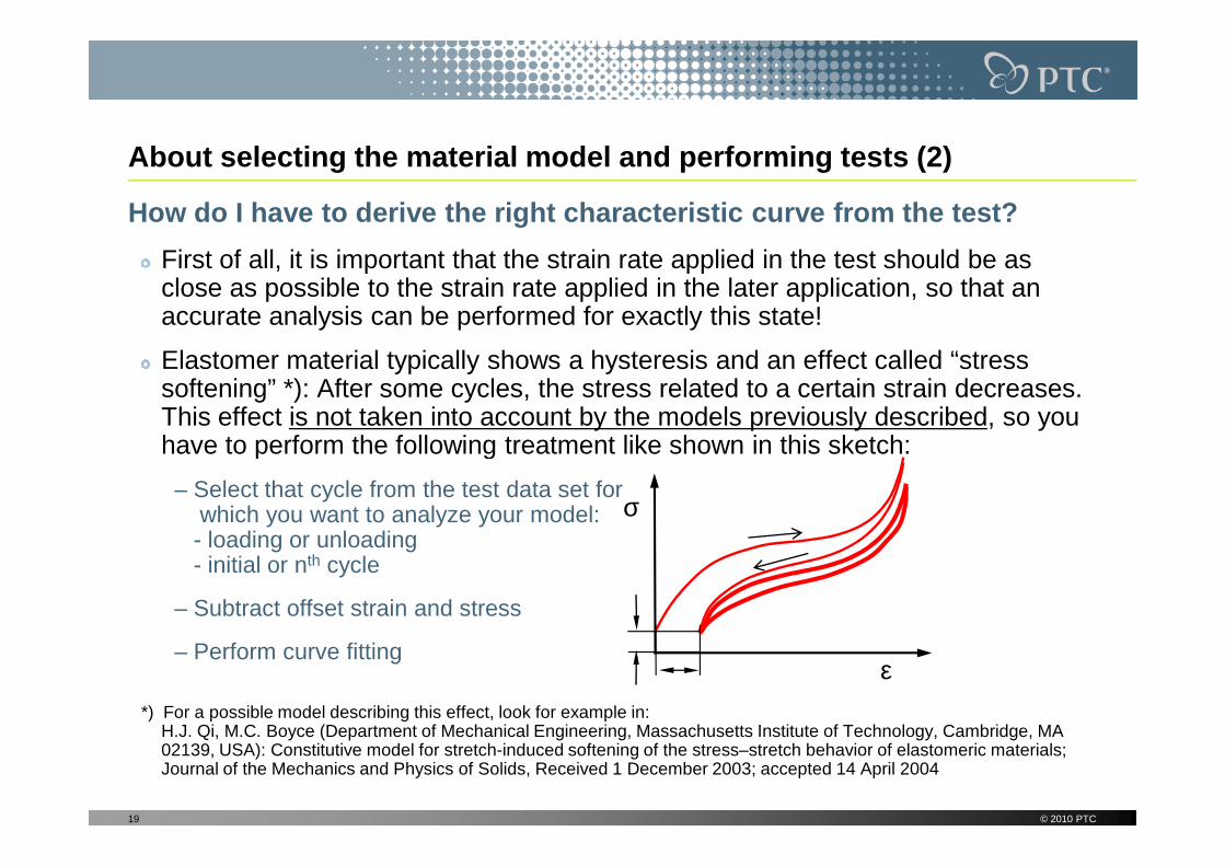
How do I have to derive the right characteristic cu rve from the test?
First of all, it is important that the strain rate applied in the test should be as close as possible to the strain rate applied in the later application, so that an accurate analysis can be performed for exactly this state!
Elastomer material typically shows a hysteresis and an effect called “stress softening” *): After some cycles, the stress related to a certain strain decreases. This effect is not taken into account by the models previously described, so you have to perform the following treatment like shown in this sketch:have to perform the following treatment like shown in this sketch:
– Select that cycle from the test data set for which you want to analyze your model:- loading or unloading- initial or nth cycle
– Subtract offset strain and stress
– Perform curve fitting
*) For a possible model describing this effect, look for example in: H.J. Qi, M.C. Boyce (Department of Mechanical Engineering, Massachusetts Institute of Technology, Cambridge, MA 02139, USA): Constitutive model for stretch-induced softening of the stress–stretch behavior of elastomeric materials; Journal of the Mechanics and Physics of Solids, Received 1 December 2003; accepted 14 April 2004
19 © 2010 PTC
ε
σ

Implementation of hyperelastic material laws in Mech anica (1)
General remarks:
Mechanica uses p-order finite element implementation to analyze hyperelasticmaterials. One of the advantages is that no special procedure is needed when the Poisson's ratio approaches to 0.5
Literature sources for high-order finite element method can be found in the book “Finite Element Analysis” by Barna Szabo and Ivo Babuska. Specifically, on page 188, “In p-extension, the rate of converge (energy norm) is not affected by page 188, “In p-extension, the rate of converge (energy norm) is not affected by Poisson's ratio.” And on page 209, “Hence, locking does not occur. The elements can deform while preserving constant volume.“
Handling of nearly incompressible material in Mecha nica:
If the value specified for D1=2/K0 is less than 1/500G0, Mechanica uses this value as limit for D1. So, we obtain for the maximum possible Poisson’s ratio used to “approximate ideal incompressibility”:
Remark: In linear elastic material analysis, the max. possible Poisson ratio Mechanica supports is 0.4999
© 2010 PTC20
4995,03001
1499
)1(2
1000
)21(31000
2 000
10 ≈=⇒
+=
−⇒== ν
ννEE
GD
K
Implementation of hyperelastic material laws in Mech anica (2)
Supported model/element types for hyperelastic mater ial analysis:
Large displacement analysis (LDA) is required for hyperelastic material analysis. All model/element types that support LDA also support hyperelastic material:
• 3D volumes
• 2D plane stress
• 2D plane strain• 2D plane strain
• 2D axial symmetry (will be supported in Wildfire 6)
• Actually no support of beams and shells
LDA: The forces and moments are equated iteratively at the deformed structure, as opposed to to SDA (small displacement analysis). Hence, an iterative procedure must be used to solve the nonlinear matrix equation for static analysis K(u,f).u=f
Mechanica uses a modified Newton-Raphson procedure for this. To increase speed, BFGS (Broyden–Fletcher–Goldfarb–Shanno method) is used so that the stiffness matrix does not have to be computed and decomposed as often. A line search technique is used to control step size (reference: Bather, Klaus-Jürgen, Finite Element Procedures in Engineering Analysis, Prentice-Hall 1982)
© 2010 PTC21

Implementation of hyperelastic material laws in Mech anica (3)
Achieving convergence of the nonlinear matrix equat ion K(u,f) .u=f using Newton-Raphson technique:
Before convergence we can calculate the residual error corresponding to the latest solution of the displacement vector u: r=f-Ku. Here, the residual vector r, has the dimensions of force (this force must be zero for system convergence). The Newton-Raphson solution then solves for Kdu=r to determine the change in u in the next iteration.
The residual norm is the dot product r.du. It can be thought of physically as a residual energy, which should be zero when we're converged. We normalize the residual norm with the dot product of the total displacement and the total force vector, so the residual norm is: (r.du)/(u.f).
This residual norm must be smaller than the default value of 1.0E-14 to achieve convergence for the "Residual Norm Tolerance" in Mechanica (see .pas-file)
Further reading: Crisfield, M: Nonlinear Finite Element Analysis of Solids and StructuresWiley, 1991, p 254.
© 2010 PTC22

Defining hyperelastic material parameters in Mechani ca (1)
The user has the following three options to define hyperelasticity:
Select one of the 6 implemented material models and enter the necessary material constants manually
Enter test data. Mechanica uses a Least Square Fitting algorithm (minimizing the normalized stress errors) to calculate the constants from the input test data for each material model. Then select the material model manually
Let Mechanica automatically choose the material model with the best fit in the test domain based on the Root Mean Stress error
Check of the different material models from test da ta input:
Mechanica performs a check on the stability of the material for six different forms of loading for 0.1≤λ≤10.0 in intervals of ∆λ=0.01. The forms of loading are:
– Uniaxial tension and compression
– Equibiaxial tension and compression
– Planar tension and compression
For each loading type and λ, the tangential stiffness D must be >023 © 2010 PTC

Defining hyperelastic material parameters in Mechani ca (2)
Treating material model instability
If an instability is found, Mechanica marks the model in the test data form with an exclamation mark and will not select it automatically (even though it may have a very small RMS error!)
If the user overrides this by manually selecting the instable material model, Mechanica issues a warning message with the values of ε for which instability is observed (-0.9≤ε ≤9.0)the values of ε1 for which instability is observed (-0.9≤ε1≤9.0)
The model may be used just up to these limits, otherwise the analysis will fail!
The following four types of tests are supported:
Uniaxial: Uniaxial tension
Biaxial: Equibiaxial tension
Planar: A certain plain strain condition (as described later)
Volumetric: Hydrostatic pressure
These stress/strain & stretch states are depicted on the next slide, respectively
24 © 2010 PTC

Defining hyperelastic material parameters in Mechani ca (3)
Uniaxial: ε1
ε2
ε3
23
22
1
11
λλλ == σ1
Idealized stress/strain states of the four hyperelast ic material tests supported in Mechanica:
Planar:
1,1
32
1 == λλ
λε1
ε2
σ1σ3
Remark: Stresses (red) or strains (blue) where no arrow is shown are Zero!
Equibiaxial:
25
ε1
ε2
ε3
σ1
σ2
3
21
1
λλλ ==
Volumetric:
13/1321 ≤=== Jλλλ
σ3(σ3 is positive because of lateral strain suppression in 3-direction, but not applied as external force like σ1)
ε1
ε2
ε3
σ1
σ2
σ3(hydrostatic pressure p=σ1=σ2 =σ3)
© 2010 PTC
Defining hyperelastic material parameters in Mechani ca (4)
Obtaining the material constants C ij and D k from the test data input:
From the uniaxial, equal biaxial, and planar tests, only the Cij are determined. The material is assumed to be incompressible, if no additional volumetric test data is given! In this case, the Dk's are shown as 0 (meaning incompressible). Remember, the engine assumes a nearly incompressible material then and uses D1 = 1/(500 G0) during the analysis like previously described (means ν=0.4995)
From the volumetric test, only the D 's are being estimated; in this case of From the volumetric test, only the Dk's are being estimated; in this case of course, incompressibility is not assumed. The Cij cannot be calculated from this test because hydrostatic pressure just creates a volume change and no shape change! That’s why a volumetric test alone is not sufficient to characterize hyperelastic material
If more than one test is entered, then the data from all of the tests are considered when determining the material properties. No one test counts more than any of the others; all tests are considered equally
Important Remark:In general, engineering (nominal) values have to be entered for stress and strain into the test data forms!
26 © 2010 PTC
Test set-ups and specimen shapes of the supported m aterial tests (1)
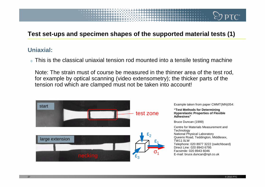
Uniaxial:
This is the classical uniaxial tension rod mounted into a tensile testing machine
Note: The strain must of course be measured in the thinner area of the test rod, for example by optical scanning (video extensometry); the thicker parts of the tension rod which are clamped must not be taken into account!
27 © 2010 PTC
start
necking
large extension
Example taken from paper CMMT(MN)054:
“Test Methods for Determining Hyperelastic Properties of Flexible Adhesives”
Bruce Duncan (1999)
Centre for Materials Measurement and TechnologyNational Physical LaboratoryQueens Road, Teddington, Middlesex, TW11 0LWTelephone: 020 8977 3222 (switchboard)Direct Line: 020 8943 6795Facsimile: 020 8943 6046E-mail: [email protected]
ε1
ε2
ε3
σ1
test zone

Test set-ups and specimen shapes of the supported m aterial tests (2)
Biaxial:
This is a disk under equibiaxial tension. The specimen mounted into a “scissor” fixture for an uniaxial testing machine and the stress state may look as follows:
For this specimen type, failure will occur in the edges where the load is
28 © 2010 PTC
test zone
edges where the load is introduced
ε1
ε2
ε3
σ1
σ2
Reference: CMMT(MN)054
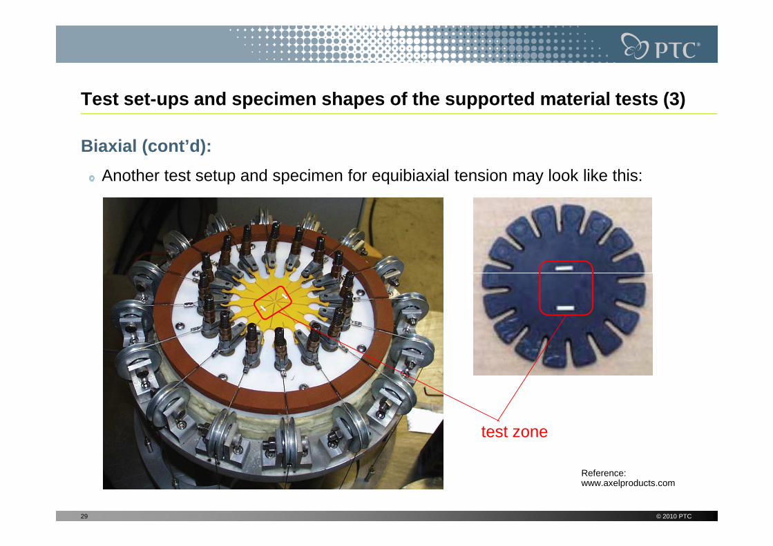
Test set-ups and specimen shapes of the supported m aterial tests (3)
Biaxial (cont’d):
Another test setup and specimen for equibiaxial tension may look like this:
29 © 2010 PTC
test zone
Reference:www.axelproducts.com

Test set-ups and specimen shapes of the supported m aterial tests (4)
Planar:
A thin sheet of hyperelastic material is clamped, so that lateral strains are prohibited here, and pulled!
ε1
ε2
Acc. to ref. CMMT(MN)054, the planar test results shall be relatively insensitive to the grip separation “d”, but this should be treated with care for larger strains. See the planar test example in part 2 of this
d
30 © 2010 PTC
test zone
σ1
σ3
F
F
lateral strain ε3=0 because of clamping!
example in part 2 of this presentation!
Reference: CMMT(MN)054

Test set-ups and specimen shapes of the supported m aterial tests (5)
Volumetric
A volumetric test setup like this compresses a cylindrical elastomerspecimen constrained in a stiff fixture
The actual displacement during compression is very small and great care must be taken to measure only the must be taken to measure only the specimen compliance and not the stiffness of the instrument itself
The initial slope of the resulting stress-strain function is the bulk modulus. This value is typically 2-3 orders of magnitude greater than the shear modulus for dense elastomers
31 © 2010 PTC
Reference:www.axelproducts.com

The uniaxial compression test (1)
Simple compression:
Biggest problem of this test is that lateral strains are disturbed by friction effects
From the analysis results shown below, one can conclude that even very small levels of friction significantly affect the measured stiffness. Furthermore, this effect is apparent at both low and high strains. This is particularly troubling because low and high strains. This is particularly troubling because friction values for elastomers are typically a function of normal force and are not well characterized
As such, the experimental compression data cannot be corrected with a significant degree of certainty
Unfortunately, both tension andcompression information is valuable to obtain because unlike some metal material models, elastomers behave very differently in compression thanin tension!
32 © 2010 PTC
Reference: www.axelproducts.com
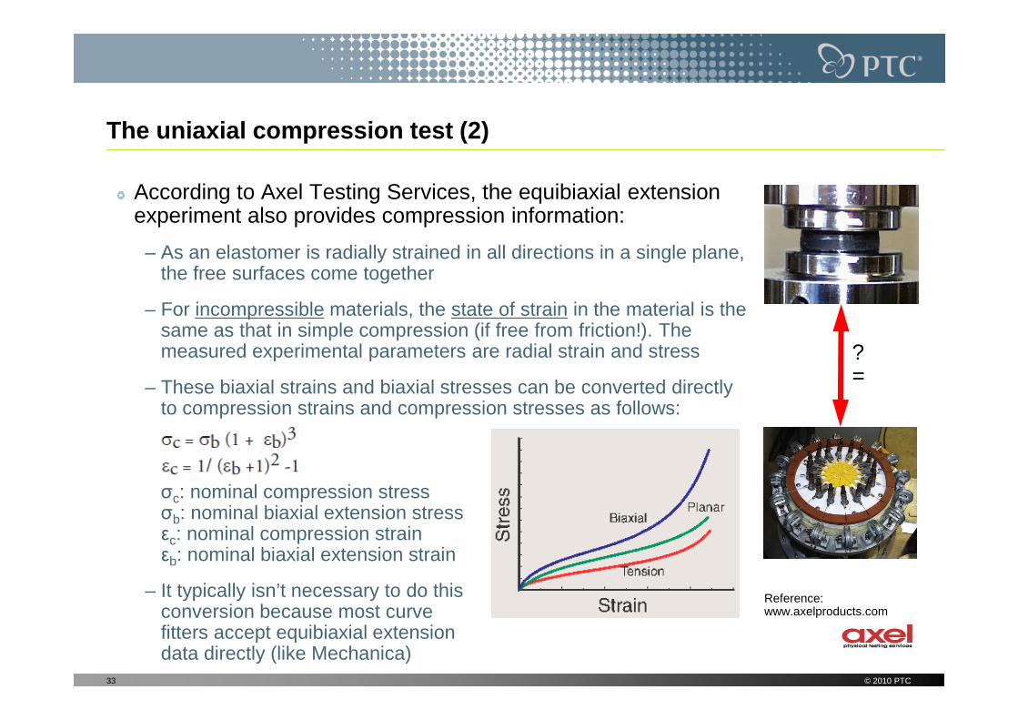
The uniaxial compression test (2)
According to Axel Testing Services, the equibiaxial extension experiment also provides compression information:
– As an elastomer is radially strained in all directions in a single plane, the free surfaces come together
– For incompressible materials, the state of strain in the material is the same as that in simple compression (if free from friction!). The measured experimental parameters are radial strain and stress ?measured experimental parameters are radial strain and stress
– These biaxial strains and biaxial stresses can be converted directly to compression strains and compression stresses as follows:
σc: nominal compression stressσb: nominal biaxial extension stressεc: nominal compression strainεb: nominal biaxial extension strain
– It typically isn’t necessary to do this conversion because most curve fitters accept equibiaxial extension data directly (like Mechanica)
33 © 2010 PTC
Reference:www.axelproducts.com
?=
Stress and strain definitions in the Mechanica LDA a nalysis (1)
Material test definitions:
Remember: In Mechanica, engineering (nominal) values have to be entered for stress and strain into the hyperelastic test data forms!
Analysis results:
Mechanica reports true stresses in the LDA analysis (in SDA of course, nominal values are output: There is no significant difference between true and nominal values are output: There is no significant difference between true and nominal stress!)
Unlike for the test definitions, Mechanica does not use engineering strains in LDA. Mechanica reports the so called “Eulerian” or “Almansi” strain, which becomes surprisingly small for large nominal tension strains and very big for large negative strains (theoretic maximum for infinite nominal tension strain is just 0.5!)
The reason is that this strain is defined with respect to the current configuration (stretched length l1) of the body – not the initial length l0!
For further explanation, the next slide shows the equations for the different strain definitions
34 © 2010 PTC

Stress and strain definitions in the Mechanica LDA a nalysis (2)
Strain definitions:
There are multiple choices for reporting strain in large deformation problems (Reference for example: B. R. Seth. Generalized strain measure with applications to physical problems. In D. Abir M. Reiner, editor, Second-Order Effects in Elasticity, Plasticity and Fluid Dynamics, pages 162–172. Pergamon Press, Oxford, 1964.)
The various strain measures have the following values for a tensile rod (l0 is the initial length, l1 is the current length):
lll ∆−– Infinitesimal, “engineering” or Cauchy strain:
(for small displacement problems only)
– Logarithmic (“natural”, “true”, “Hencky”) strain:(obtained by integrating the incremental strain)
– Green-Lagrange Strain:(defined with respect to the initial configuration)
– Eulerian (Almansi) Strain:(defined with respect to the deformed configuration)
35 © 2010 PTC
00
01
l
l
l
ll ∆=−=ε
...432
)1ln(
lnln
432
0
1
11
1
0
−+−+−=+=⇔
=
=⇒
∂=∂⇒∂=∂ ∫ ∫
εεεεεε
λεεε
L
L
l
lLL l
l
l
l
l
l
20
20
21
2
1
l
llG
−=ε
21
20
21
2
1
l
llE
−=ε

Stress and strain definitions in the Mechanica LDA a nalysis (3)
Graphical representation of the different strains:
101 −=−= λε ll
20
20
21
2
1
l
llG
−=ε
stra
in
36 © 2010 PTC
10
−== λεl
( ) λε ln/ln 01 == llL
21
20
21
2
1
l
llE
−=ε
stretch λ=l1/l0Reported by Mechanica in LDA!

Part 2
Application examples
© 2010 PTC37

A test specimen subjected to uniaxial load (1)
Test specimen and test data:
Provided uniaxial test data (engineering values) of an example elastomer:
Test specimen acc. to DIN 53504-S2
38 © 2010 PTC
Loaded cross section is 8 mm2
Test specimen acc. to DIN 53504-S2
R12.5

A test specimen subjected to uniaxial load (2)
For the Arruda-Boyce model, the Least Square Fitting algorithm failed, so it cannot be used (and is not displayed)
The exclamation mark means, that for a certain strain range, the model is unstable (Zero tangent stiffness)
39 © 2010 PTC
entered test data(engineering values)
tangent stiffness)
Mechanicaautomatically selects “Polynomial Order 2” – model as best fit to test data
The “D”-values are shown as zero (=incompressible), since no volumetric test has been specified. However, internally Mechanicauses D1=D2= 1/(500G), which corresponds to a Poisson ratio of 0.4995
If this box is unchecked, you can manually enter the coefficients for the material law and compare them with the test points in the graph
G0= 2(C10+C01)=3.11234 MPa
K0=2/D1=3112.34 MPa (ν=0,4995!)
� E0=2G0(1+ν)= 9.3339077 MPa

A test specimen subjected to uniaxial load (3)
Model Set-Up
There are different ways to set up the FEM-model of the specimen:
– The most “realistic” one is to use the complete specimen geometry from Pro/E, prepare and mesh it, define the material and run the analysis. This looks of course nicest
– However, to save time we will just run an eighth part of the measurement-zone of the model with symmetry constraints, containing just three bricks (you could also use 2D plane stress of course!). This analysis will run very fast!plane stress of course!). This analysis will run very fast!
We create some measures to determine the engineering values for stress and strain, since the Mechanica engine reports only true stress and Almansi strain:
– A measure for nominal strain, using the following formula that derives the engineering strain ε from the Eulerian (Almansi) strain εE output by Mechanica:
– As cross-check, a measure for nominal strain, derived from the specimen length change devided by the initial length (with help of a Mechanica computed measure)
– A computed measure for nominal stress, using the constraint reaction force divided by the initial cross section
40 © 2010 PTC
121
1
1
11
2
1
2
12
21
20
21 −
−=⇔
+−=−=
EE
l
ll
εε
εε
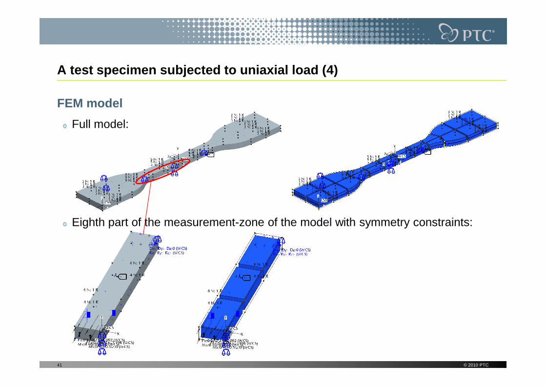
A test specimen subjected to uniaxial load (4)
FEM model
Full model:
Eighth part of the measurement-zone of the model with symmetry constraints:
41 © 2010 PTC

Results (displacement magnitude, deformed shape in scale)
Full model:
A test specimen subjected to uniaxial load (5)
Eighth part of the measurement-zone of the model with symmetry constraints:
Eighth part just with linear behavior (small strain solution and properties):
42 © 2010 PTC

Stress-strain-curves of the exampleelastomer
A test specimen subjected to uniaxial load (6)
43 © 2010 PTC
Here, a good match between the linear and hyperelastic material model is just prevailing below strains of approx. 5%!

Engineering stress and strain versus stretch
A test specimen subjected to uniaxial load (7)
44 © 2010 PTC
Almansi strain goes for theoretical limit of 0.5(0.491 for max. load applied)

A volumetric compression test (1)
Test specimen and test data:
Like shown in the section about material tests, in a volumetric test a cylindrical specimen is uniaxial compressed while it is constrained in a very stiff fixture
From Hooke’s law, we have with σ1=σax=F/A, σ2=σ3=σq and ε2=ε3 =0:
( ){ } 211
3211 =
−⋅=+−⋅= axqA
F
EEενσσσνσε
So, we have two different equations to solve for the two unknown quantities σq and εax. We obtain:
45 © 2010 PTC
( ){ }
( ){ } 011
011
2133
3122
==
+−⋅=+−⋅=
==
+−⋅=+−⋅=
qqq
qqq
A
F
EE
A
F
EE
AEE
εσνσσσνσε
εσνσσσνσε
−−=
−=
ννε
ννσ
121
1
12
A
F
E
A
F
ax
q
σax
σq σq
σax
εax
εax
A volumetric compression test (2)
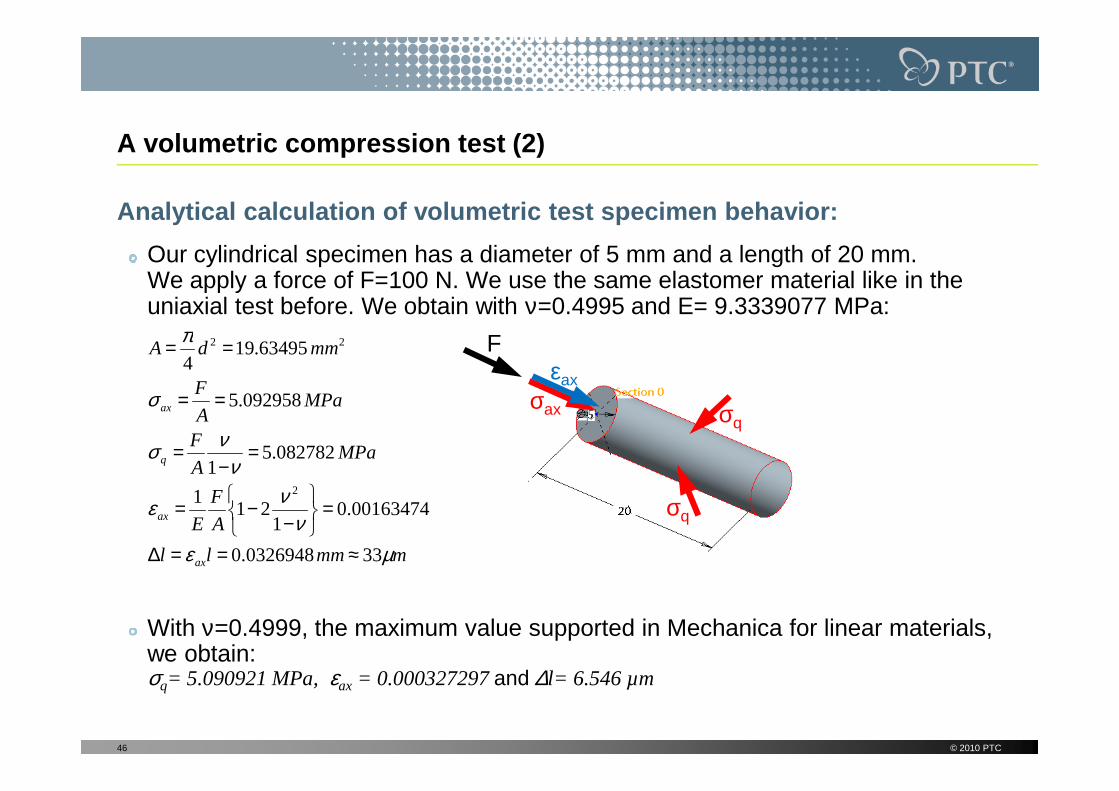
Analytical calculation of volumetric test specimen behavior:
Our cylindrical specimen has a diameter of 5 mm and a length of 20 mm. We apply a force of F=100 N. We use the same elastomer material like in the uniaxial test before. We obtain with ν=0.4995 and E= 9.3339077 MPa:
MPaF
mmdA
σ
π
092958.5
63495.194
22
==
==
σεax
F
With ν=0.4999, the maximum value supported in Mechanica for linear materials, we obtain: σq= 5.090921 MPa, εax = 0.000327297 and ∆l= 6.546 µm
46 © 2010 PTC
mmmll
A
F
E
MPaA
F
MPaA
F
ax
ax
q
ax
µεν
νε
ννσ
σ
330.0326948
0.001634741
211
082782.51
092958.5
2
≈==∆
=
−−=
=−
=
== σax σq
σq

A volumetric compression test (3)
Comparison of hyperelastic material with steel:
If we compress a steel cylinder with the same dimensions, we obtain with E=210000 MPa for the unconstrained condition (σq =0):
With ν=0,3 we obtain (constrained condition ε =0):
mdE
Fl
EA
Fll
lKFlEAK
µπ
485.04
;/
2===∆
∆==σax
εax
εq
εq
unconstrained
With ν=0,3 we obtain (constrained condition εq =0):
σq=2.183 MPa, εax=1.8016 E-5 and ∆l=0.36 µm
Because of the compressibility of steel, there is not a big difference to the unconstrained condition (factor ≈1,35)!
The elastomer cylinder, assuming ν=0.4999, deforms just 18 times more (∆l= 6.546 µm) than the steel cylinder,even though its E-modulus is approx. 22500 times lower!
�Elastomer material can behave surprisingly stiff undercertain conditions! Take this into account when designing for example “soft” rubber layers to homogenize bearing stress!
47 © 2010 PTC
εq
σax σq
σq
εax
constrained

σax σq
σq
εax
A volumetric compression test (4)
Model Set-Up:
Since we have for this condition just very small deformations, we could run the compression test analysis with the linear theory as 2D axial symmetric model (in WF6, 2D axial symmetric models will also support LDA and hyperelasticity)
Mechanica in this case automatically selects the initial Mechanica in this case automatically selects the initial values G0 and K0 from the example elastomer test data input (equivalent to E0=9.3339 and ν=0.4995)
However, we will run the compression test as 2D plane strain model. This is possible, since for this loading condition the axial displacement for a given axial stressis not a function of the specimen cross section, but just of its length!
In 2D plane strain, we can run the model linearizedand with LDA including hyperelasticity, to check the difference!
48 © 2010 PTC
2D plane strain

A volumetric compression test (5)
Model Set-Up:
For this simple stress state without any gradients, a very course mesh is sufficient to obtain accurate results:
Also in this model, we define a computed measure for the engineering strain to compare it with the Almansi strain reported in LDA. The difference should be negligible here!
49 © 2010 PTC

A volumetric compression test (6)
Analysis results:
As expected, the difference between analytical results, SDA with linear material data and LDA with hyperelastic material is very small for volumetric compression:Linear analysis results (Multi Pass):
max_stress_xx: -5.082782e+00 0.0%
max_stress_yy: -5.092958e+00 0.0%
max_stress_zz: -5.082782e+00 0.0% MPaF
MPaA
Fax
082782.5
092958.5
==
==
νσ
σ
Linear analysis results (analytical solution):
50 © 2010 PTC
max_stress_zz: -5.082782e+00 0.0%
strain_energy: 2.081421e-01 0.0%
displacement_Y: -3.269489e-02 0.0%
epsilon_ax_eng: -1.634744e-03 0.0%mmll
A
F
E
MPaA
F
ax
ax
q
0.0326948
0.001634741
211
082782.51
2
==∆
=
−−=
=−
=
εν
νε
ννσ
LDA results with hyperelasticity (Single Pass):
max_stress_xx: -5.082742e+00
max_stress_yy: -5.092958e+00
max_stress_zz: -5.082742e+00
strain_energy: 2.077312e-01
Almansi_strain: -1.638205e-03
displacement_Y: -3.268382e-02
epsilon_ax_eng: -1.634191e-03
No significant difference!

A planar test (1)
Specimen Geometry:
We will use a thin sheet of the same example elastomer: Thickness 2 mm, clamped length 100 mm, grip separation d=30 mm
ε1
ε2
51 © 2010 PTC
test zone
σ1
σ3
F
F
lateral strain ε3=0 because of clamping!
A planar test (2)
ε1
σ1
ε2
plane strain
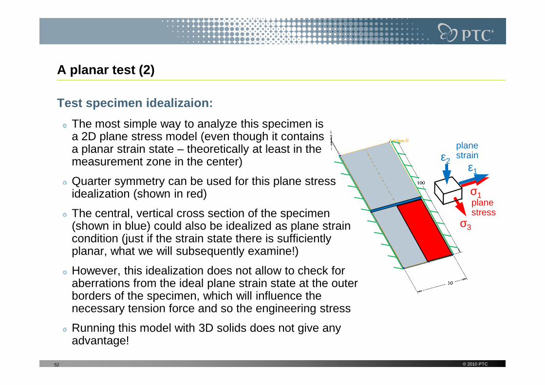
Test specimen idealizaion:
The most simple way to analyze this specimen is a 2D plane stress model (even though it contains a planar strain state – theoretically at least in the measurement zone in the center)
Quarter symmetry can be used for this plane stressidealization (shown in red)
52 © 2010 PTC
σ1
σ3
plane stress
idealization (shown in red)
The central, vertical cross section of the specimen (shown in blue) could also be idealized as plane strain condition (just if the strain state there is sufficiently planar, what we will subsequently examine!)
However, this idealization does not allow to check for aberrations from the ideal plane strain state at the outer borders of the specimen, which will influence the necessary tension force and so the engineering stress
Running this model with 3D solids does not give any advantage!
A planar test (3)
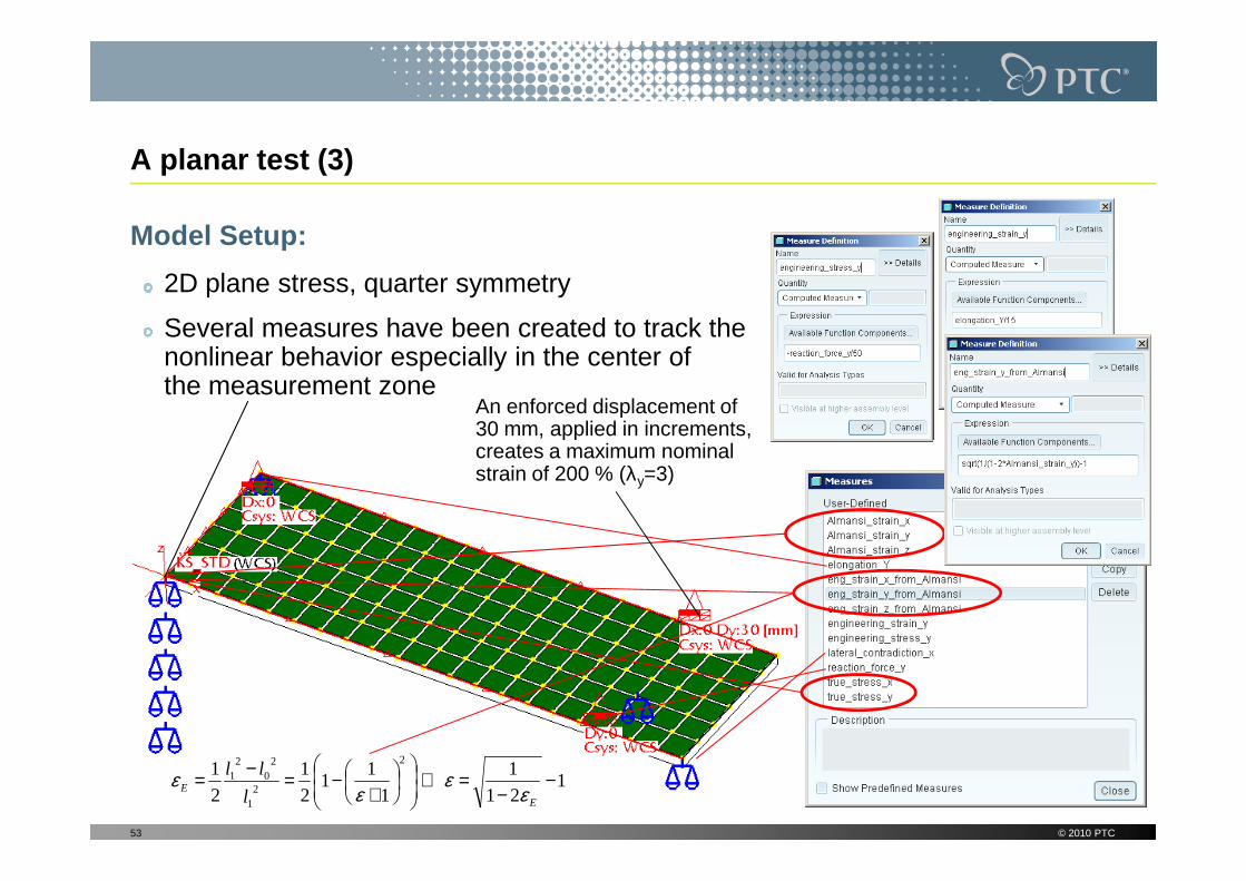
Model Setup:
2D plane stress, quarter symmetry
Several measures have been created to track the nonlinear behavior especially in the center ofthe measurement zone
An enforced displacement of 30 mm, applied in increments, creates a maximum nominal
53 © 2010 PTC
creates a maximum nominal strain of 200 % (λy=3)
121
1
1
11
2
1
2
12
21
20
21 −
−=⇔
+−=−=
EE
l
ll
εε
εε

A planar test (4)
Displacement results (in scale):
Enforced displacement:3 mm
Enforced displacement:6 mm
Enforced displacement:12 mm
54 © 2010 PTC
Enforced displacement:18 mm
Enforced displacement:24 mm
Enforced displacement:30 mm
Extreme lateral contraction!
A planar test (5)
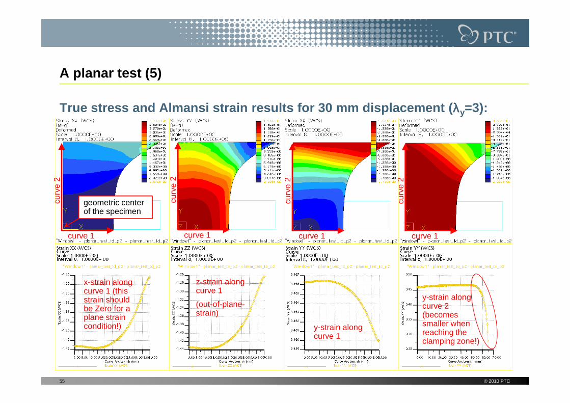
True stress and Almansi strain results for 30 mm dis placement ( λλλλy=3):
curv
e 2
geometric center curv
e 2
curv
e 2
curv
e 2
55 © 2010 PTC
curve 1
curv
e 2
x-strain alongcurve 1 (this strain should be Zero for a plane strain condition!)
z-strain alongcurve 1
(out-of-plane-strain)
y-strain alongcurve 1
y-strain alongcurve 2 (becomes smaller when reaching the clamping zone!)
geometric center of the specimen
curve 1
curv
e 2
curve 1
curv
e 2
curve 1
curv
e 2

A planar test (6)
Strain results versus stretch in the geometric cent er of the specimen:
These strains are the y-values for the geometric center of the specimen (in the measurement zone, see test setup description)
56 © 2010 PTC
Here, the “nominal” engineering strain in y is the “averaged” strain from the total specimen elongation under y-load
The graph shows engineering and Almansistrains for comparison

A planar test (7)
Engineering strain results vs. stretch in the speci men geometric center:
These graphs show engineering strains only, because this is more familiar for most users!
57 © 2010 PTC
We have an approximate plane strain condition just under very small loads! (green line = x-strain should be Zero for all stretch values to have a true plane strain condition!)
For higher loadings, we obtain more and more a uniaxialstress & triaxial strain state in the measurement zone!

A planar test (8)
Conclusions:
In nonlinear analysis of hyperelastic material, the stress and strain state quality (type) may vary significantly during the analysis, not only the quantity like in linear analysis with metals
In the example shown, at the beginning we have a plane strain and plane stress condition (plane conditions in different planes, respectively). When the stretch is increasing, we obtain in the center of the specimen, where we measure the
58 © 2010 PTC
increasing, we obtain in the center of the specimen, where we measure the strains, more and more a uniaxial stress and a triaxial strain state, which of course is something that we don’t want to have!
Hence, great care must be taken when defining multiaxial test geometry and load levels!
For a precise test evaluation, also FEM analyses are recommended to understand the specimen behavior. Mechanica can help you a lot here!

Influence of the Material Law (1)
Motivation:
Until now, all example analyses were based on the same simple uniaxial tension test and the “polynomial order 2” hyperelastic material model
For comparison, we will now also examine the influence of
– the material law used: We will run some example analyses not only with the proposed (“automatic - best fit”) model, but also with that one on the list with the second smallest RMS-error;
59 © 2010 PTC
RMS-error;
– the stress and strain state (uniaxial or planar test)
Goal:
Obtain a “feeling” for how sensitive our analyses and predictions are against such changes
Learn what to do to minimize errors

Influence of the Material Law (2)
Material law influence
We select the best and second best material law for the test data fit (see RMS error) and re-run both uniaxial and planar test, respectively
60 © 2010 PTC
Polynomial order 2 model delivers lowest RMS error and is therefore automatically proposed by Mechanica
The Yeoh model has to be selected manually

max_disp_mag: 8.100103e+01max_disp_x: 1.266057e+00max_disp_y: -6.330287e-01max_disp_z: 8.098866e+01max_prin_mag: 6.717262e+01max_stress_prin: 6.717263e+01max_stress_vm: 6.717262e+01max_stress_zz: 6.717262e+01strain_energy: 7.238702e+02Almansi_strain: 4.910613e-01engineering_strain_from_Almansi: 6.479093e+00engineering_strain_from_dL: 6.479093e+00engineering_stress_from_Freac: 9.046000e+00length_change: 8.098866e+01
Influence of the Material Law (3)
Uniaxial Test Case
We run the uniaxial model again for the tension case. The differences are very low in this case, like expected!
Mea
sure
res
ults
of p
olyn
omia
l or
der
2 m
ater
ial m
odel
max_disp_mag: 8.065296e+01max_disp_x: 1.261583e+00max_disp_y: -6.307917e-01max_disp_z: 8.064063e+01max_prin_mag: 6.636112e+01max_stress_prin: 6.636112e+01max_stress_vm: 6.636112e+01max_stress_zz: 6.636112e+01min_stress_prin: -4.307335e-07strain_energy: 7.152915e+02Almansi_strain: 4.909944e-01engineering_strain_from_Almansi: 6.451250e+00engineering_strain_from_dL: 6.451250e+00engineering_stress_from_Freac: 9.046000e+00length_change: 8.064063e+01reaction_force: -1.809200e+01true_tension_stress: 6.636112e+01
length_change: 8.098866e+01reaction_force: -1.809200e+01true_tension_stress: 6.717263e+01
61 © 2010 PTC
Mea
sure
res
ults
of p
olyn
omia
l or
der
2 m
ater
ial m
odel
Mea
sure
res
ults
of Y
eoh
mat
eria
l mod
el
Test data for comparison

Planar Test Case
We run the planar model again. The differences are unexpectedly very big!(see some extreme cases in red)max_disp_mag: 3.000000e+01max_disp_x: -2.421340e+01max_disp_y: 3.000000e+01max_disp_z: 0.000000e+00
max_disp_mag: 3.000000e+01max_disp_x: -7.410746e+00max_disp_y: 3.000000e+01max_disp_z: 0.000000e+00max_prin_mag: 2.368579e+01
Influence of the Material Law (4)M
easu
re r
esul
ts o
f pol
ynom
ial o
rder
2 m
ater
ial m
odel
max_disp_z: 0.000000e+00max_prin_mag: 4.290650e+01max_stress_prin: 4.290650e+01max_stress_vm: 3.942243e+01max_stress_xx: 3.737426e+01max_stress_xy: 1.268577e+01max_stress_yy: 1.540157e+01min_stress_prin: -2.106141e+00strain_energy: 8.355114e+03Almansi_strain_x: -1.411463e+00Almansi_strain_y: 4.663071e-01Almansi_strain_z: -1.434179e+00elongation_Y: 3.000000e+01eng_strain_x_from_Almansi: -4.885514e-01eng_strain_y_from_Almansi: 2.852263e+00eng_strain_z_from_Almansi: -4.915635e-01engineering_strain_y: 2.000000e+00engineering_stress_y: 7.817140e+00lateral_contraction_x: -2.421340e+01reaction_force_y: -3.908570e+02true_stress_x: 8.544871e-01true_stress_y: 1.538512e+01
max_disp_z: 0.000000e+00max_prin_mag: 2.368579e+01max_stress_prin: 2.368579e+01max_stress_vm: 2.343005e+01max_stress_xx: 1.058007e+01max_stress_xy: 1.148228e+01max_stress_yy: 1.362583e+01min_stress_prin: -4.675187e-02strain_energy: 6.872396e+03Almansi_strain_x: -2.145352e-02Almansi_strain_y: 4.444555e-01Almansi_strain_z: -3.791858e+00elongation_Y: 3.000000e+01eng_strain_x_from_Almansi: -2.078693e-02eng_strain_y_from_Almansi: 2.000299e+00eng_strain_z_from_Almansi: -6.586795e-01engineering_strain_y: 2.000000e+00engineering_stress_y: 7.139334e+00lateral_contraction_x: -7.410746e+00reaction_force_y: -3.569667e+02true_stress_x: 1.015148e+00true_stress_y: 1.070790e+01
62 © 2010 PTC
Mea
sure
res
ults
of p
olyn
omia
l ord
er 2
mat
eria
l mod
el
Mea
sure
res
ults
of Y
eoh
mat
eria
l mod
el
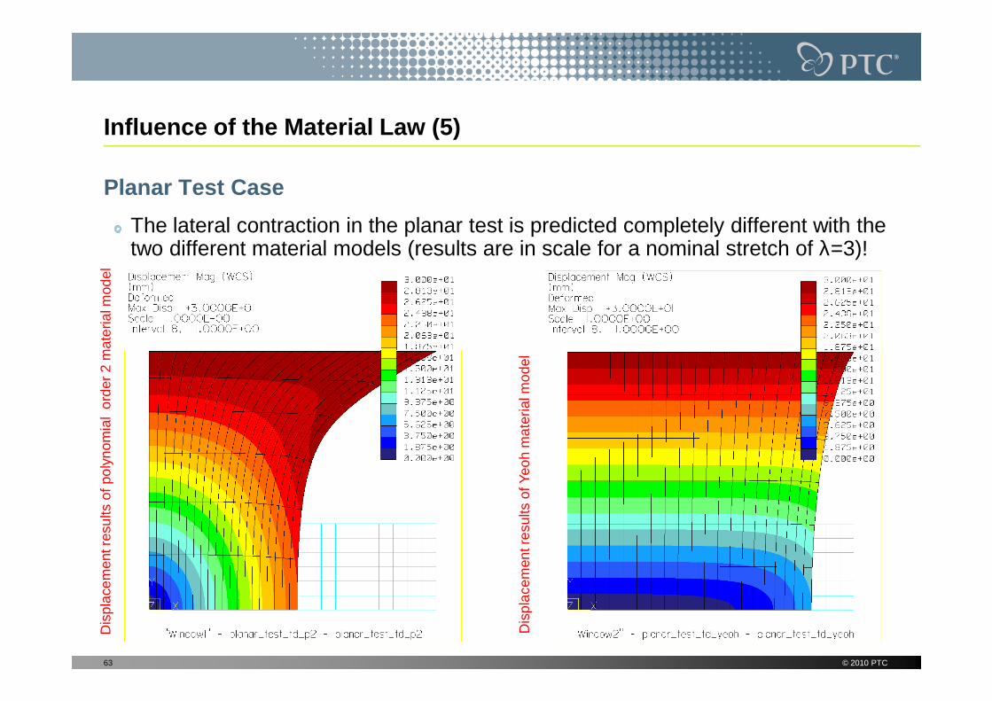
Influence of the Material Law (5)
Planar Test Case
The lateral contraction in the planar test is predicted completely different with the two different material models (results are in scale for a nominal stretch of λ=3)!
Dis
plac
emen
t res
ults
of p
olyn
omia
l or
der
2 m
ater
ial m
odel
63 © 2010 PTC
Dis
plac
emen
t res
ults
of p
olyn
omia
l or
der
2 m
ater
ial m
odel
Dis
plac
emen
t res
ults
of Y
eoh
mat
eria
l mod
el
Influence of the Material Law (6)
Conclusions:
The difference in the lateral contraction cannot be explained with a different bulk modulus (means different Poisson ratios): For both models, since no volumetric tests have been performed, so the Di are set to Zero (internally D0=1/500 G0, this means the same Poisson ratio of 0.4995 is used both models)
The Yeoh model neglects the second stretch invariant in the strain energy density function, just the first one is used, which may explain the difference
64 © 2010 PTC
function, just the first one is used, which may explain the difference
With this example, it becomes clear that the test conditions (uniaxial, planar…) highly influence the usability of test data for the analysis of the real design:A simple tension test is often not enough for a good prediction of your real part behavior if this not loaded in simple tension as well!
In general, do as many different tests as possible to characterize your material!
Especially use test conditions as close as possible to the loading state of the part you want to design!
023
21
23
22
22
212
23
22
211
=++=
++=
λλλλλλ
λλλ
I
I!

Thanks for your attention!
© 2010 PTC65

PTC Simulation Services Introduction
PTC Global Services provides services for our own simulation products:
– Pro/ENGINEER Mechanica as a FEA tool with p-method for structural mechanical, thermal and thermo-mechanical analysis
– Pro/ENGINEER MDX and MDO (Mechanism Design Extension and Mechanism Dynamics Option) for kinematic and dynamic multi-body simulations
The benefits are accomplished as following:
– Required calculations
© 2009 PTC66
– Required calculations
– Development of the required analysis and optimization, working with the design team, directly on the working CAD data, including adoption of mechanical systems engineering tasks
– On-site simulation consulting � Software and calculation method knowledge transfer
– Simulation training and workshops from PTC University
The following slides show the newest examples of simulation project and education references. Numerous other references from other clients and to other simulation issues can be provided upon request.

� During the development of new observation systems, Zeiss Optronics performs analyses to study the behavior of the installed subsystems for assuring that the final product works accurately. For the subsystem shown to the right, PTC Global Services was charged with these examinations
� PTC built up the dynamic analysis model in Mechanica
BUSINESS INITIATIVE
PTC Global Services Examines the Dynamic Structural Behavior of an Opto-Mechanical Subsystem Prototype from Carl Zeiss Optronics with Pro/ENGINEER® Mechanica ® Software
SOLUTION
Electronics & High Tech
Carl Zeiss Optronics GmbH, a member of the Carl Zeiss Group located in Oberkochen, Germany, develops and produces high-precision and robust opto-electronic systems for observation and defense purposes. For such products exposed to intense loading, advanced system analysis with the Finite Element Method is an integral part of the product development.
© 2006 PTC67
“The dynamic analysis study gave us a very good und erstanding of exactly what happens in our newly des igned subassembly for moving lens elements. PTC’s respons ible consultant for the project, Dr. Roland Jakel, also provided excellent ideas for helpful design modific ations. With the obtained knowledge, we can now enh ance the subsystem in a very early stage of the development, ensuring that it meets the requirements.”
Dr.-Ing. Thomas Meenken, Team Leader Simulation, Ca rl Zeiss Optronics GmbH
© 2010 PTC
� PTC built up the dynamic analysis model in Mechanica with the help of given Zeiss Pro/ENGINEER CAD model assembly data. Reasonable linearizations were developed for the guiding system and the preloaded drive mechanism. Their validity was strictly controlled during all subsequent analyses. Given sine sweep test data was compared with the dynamic frequency analysis results to assure an accurate mathematical model of the subsystem
� Good match of test and analysis result data helped to understand the dynamic characteristics of the subsystem
� Points in the design leading to unwanted behavior could be identified and solutions were provided
RESULT
Top Left: The meshed Mechanica FEM model derived by PTC from the Zeiss Pro/ENGINEER data set, showing the p-elements and idealizations
Top Middle: Pro/ENGINEER assembly model of the optical subsystem showing the dynamic test setup with several attached 3-axis acceleration sensors
Bottom Left: A typical modal shape of the opto-mechanical subsystem attached to a linear roller bearing
Bottom Middle: Frequency response curves in the domain of interest showing good match of measured and analyzed accelerations (sine sweep test vs.Mechanica dynamic frequency analysis)
Bottom Right: Integrated 1-sigma displacement response density functions allowing to judge which frequencies deliver high fractions to the deposition of the optical group of interest (Mechanica random response analysis)

Otto Bock HealthCare is the leading supplier of innovative products for people with restricted mobility, and, as a recognizedsystem provider of high-quality, technologically advanced products and services, it is also the global leader in orthopedic technology. The company was founded in Berlin in 1919, and is now led by Professor Hans Georg Näder, the third-generation managing shareholder. In addition to the core competency as the leading company in the Orthobionic® field, Bionicmobility® isan additional competency of Otto Bock. It combines mobility solutions such as high-quality lightweight and active wheelchairs, power wheelchairs, and products for pediatric rehabilitation and seating shell systems.
BUSINESS INITIATIVE� The technologically advanced orthopedic products developed by
Otto Bock require extensive Finite Element analyses to ensure proper function in service over their complete life span. For a more accurate solution of nonlinear problems like contact and fastener analyses, Otto Bock wanted to deepen the
PTC University Further Educates Otto Bock HealthCar e in Advanced Nonlinear Contact and Bolt Analysis with Pro/ENGINEER ® Mechanica ® Software
Medical Devices
© 2006 PTC68 © 2010 PTC
and fastener analyses, Otto Bock wanted to deepen the knowledge of their design engineers in this demanding topic
� PTC offered an on-site workshop for these nonlinear analysis themes with the opportunity for Otto Bock engineers to get their typical product analysis tasks exemplarily solved by the PTC course instructor
� The theoretic background knowledge provided with help of the Otto Bock product examples supports the engineers in applying the Mechanica FEM code correctly to their analysis tasks
SOLUTION
“We listened well to the background information PTC provided in this course for frictionless and infin ite friction contact theory in Mechanica as well as to the extensive explanations about behavior of fasten ers. In addition, the example solutions provided help us a lot since we can apply all this directly to our new products under development.” Ralf Allermann, Development / Design / Simulation, Otto Bock HealthCare GmbH
RESULT
Right: The functional element of the Otto Bock 1C30 Trias prosthetic foot with carbon leaf springs and bolted connections containing typical simulation tasks treated in the advanced workshop
Top images : Fastener theory acc. to the German VDI 2230 guideline outlined extensively in the bolt analysis workshop
Bottom left: Pro/ENGINEER Mechanica model set-up with a carbon leaf spring bolted to an aluminum lever (one of several Otto Bock example tasks solved by PTC in the customized workshop)
Bottom middle: Mechanica analysis result of this model (comparative stress)

The Vaillant Group is an internationally operating heating, ventilation and air-conditioning technology concern based in Remscheid, Germany. As one of the world's market and technology leaders, the company develops and produces tailor-made products, systems and services for domestic comfort. The product portfolio ranges from efficient heating appliances based on customary fuels to system solutions for using regenerative energy sources. As Europe’s number one heating technology manufacturer, ‘thinking ahead’ is a culture which is embraced throughout their business. To ensure an excellent product quality and short development cycles, Vaillant uses modern CAE tools like CFD software or Mechanica as a Finite Element program.
BUSINESS INITIATIVE� During the product lifecycle, design modifications are often adopted
to decrease manufacturing costs while maintaining or increasing product quality. Also here, FEM is used to ensure the reliability of such changes. The Mechanica software knowledge of the VaillantCAx application engineers was to be extended to advanced nonlinear
PTC University Supports Vaillant in Advanced Nonlin ear Contact and Bolt Analysis with Pro/ENGINEER ® Mechanica ® Software
Consumer Products
© 2010 PTC
CAx application engineers was to be extended to advanced nonlinear simulation, so that very ambitious analysis tasks can be solved in-house without external support
� PTC offered an individual simulation workshop focusing on contact and bolt analysis theory. Original Vaillant product examples and CAD data sets were used for practical training examples
� Obtained knowledge in nonlinear contact and bolt FEM analysis
� Obtained FEM sample solutions for typical Vaillant analysis tasks, like for the screw fitting shown right, allowing own further studies
SOLUTION
“Attending the advanced PTC training in Mechanica non linear contact and bolt analysis has enabled us to do these ambitious expert analyses in the future wi thout external support. We value the excellent knowledge transfer and the sample solutions accurat ely provided on base of our own products and simulation tasks.” Stefan Schweitzer-De Bortoli, CAx Application Engine er Simulation Tools, Vaillant GmbH
RESULTRight image: A state-of-the-art Vaillant heating system for domestic comfort
Left images : Screwed joint analysis of a pipe connection with non-regular geometry, performed with Mechanica in the customized workshop: A hexagonal spigot nut (1) connects the copper tube end (2) with the brass tube (3), a sealing (4) is used against leakage of the fluid. Such bolted connections cannot be analyzed analytically acc. to bolt analysis guidelines because of their geometry; therefore Mechanica allows an accurate FEM analysis.
(1) (3) (4) (2)

Dictionary Technical English-German (1)
Most important terminology for German listeners:
bearing stress – Auflagerspannung
bulk modulus – Kompressionsmodul K = -∆p.V/∆V = E/(3(1-2ν))
coefficient of thermal expansion (CTE) – Wärmeausdehnungskoeffizient α
density – Dichte
dot (scalar) product – Skalarprodukt
hardness – Härte
modulus of elasticity – Elastizitätsmodul E
nominal (or engineering) strain – technische Dehnung ε = ∆l / l
nominal (or engineering) stress – technische Spannung σ = F / A0
poisson ratio – Querdehnzahl ν
principal axis transformation – Hauptachsentransformation
© 2010 PTC70

Dictionary English-German (2)
shear modulus – Schubmodul G = E/(2(1+ν))
strain – Dehnung ε
strain energy density function – Dehnungsenergiedichte-Funktion W (volumenbezogen)
stress softening – Entfestigung
stretch – Streckung, Längungstretch – Streckung, Längung
stretch invariants – Streckungsinvarianten I1, I2, I3stretch ratio – Streckungsverhältnis λ = ε+1
tension strength – Zugfestigkeit
volumetric ratio – relative Volumenänderung J = ∆V / V
© 2010 PTC71

Informations about the Presenter
Roland Jakel
Dipl.-Ing. for mechanical engineering (Technische Universität Clausthal)
Ph.-D. in design and analysis of engineering ceramics(FEM-Analysis and subroutine programming with Marc/Mentat)
1996-2001 Employee at Dasa in Bremen (Daimler-Benz Aerospace, Product Division Space-Infrastructure, today EADS Astrium):
© 2010 PTC72
Division Space-Infrastructure, today EADS Astrium):
– Structural simulation (FEM-Analysis with NASTRAN/PATRAN and Mechanica)
– Project management for Ariane 5 Upper Stage „ESC-A“ Subsystems (Stage Damping System “SARO”, Inter Tank Structure)
At the former DENC AG („Design ENgineering Consultants“) from 2001-2005 responsible for structural simulation services and education with the PTC simulation products (Mechanica, MDX, MDO, BMX)
Since the DENC AG acquisition by PTC in 2005, Roland Jakel is responsible for the PTC simulation services within the Global Services Organization (GSO) for CER (Central Europe)


![[S. Graham Kelly] Theory and problems of mechanica(BookZZ.org)](https://static.fdocuments.in/doc/165x107/629c9a6ef8656f4f0c687b06/s-graham-kelly-theory-and-problems-of-mechanica-.jpg)

